Instruction Manual for the Lake Michigan Chinook Salmon ... · PPRA Instruction Manual – 05-20-14...

PPRA Instruction Manual – 05-20-14

Figure 1.

Instruction Manual for the Lake Michigan Chinook Salmon-Alewife

Predator-Prey Ratio Analysis

by

Rick Clark, Mike Jones, and Iyob Tsehaye

Quantitative Fisheries Center

Department of Fisheries and Wildlife

Michigan State University, East Lansing MI 48824

May 20, 2014

Introduction

The Lake Michigan Chinook salmon-alewife predator-prey ratio analysis (PPRA) was developed

in a series of workshops in 2013 (Lake Michigan Salmonid Working Group and Collaborators 2014;

Jones et al. 2014). The purpose of this report is to provide instructions for running the PPRA.

The primary purpose of the PPRA is to monitor the Chinook salmon-alewife predator-prey

balance in the lake to help evaluate Chinook salmon stocking rates. The PPRA uses data collected by

multiple government agencies: the Departments of Natural Resources for Illinois (ILDNR), Indiana

(INDNR), Michigan (MIDNR), and Wisconsin (WIDNR), the US Geological Survey (USGS), and the US

Fish and Wildlife Service (USFWS). The overall procedure involves: 1) assembling the necessary

biological data; 2) estimating

current-year values for each of the

biological indicators and updating

the time series of historical values;

and 3) using the biological

indicators and the projection

model to judge the performance of

the stocking policy.

Biological data,

spreadsheets, Statistical Catch at

Age models (SCA), scientific

references, and these instructions

are all organized in computer files

within a main folder named “LM

PPRA – 05-20-14” (Figure 1).

The actual computer files for the

current version can be obtained

from the Chairs of the Salmonid

(SWG) or Planktivore (PWG)


Working Groups for Lake Michigan or from the Quantitative Fisheries Center (QFC), Michigan State

University.

Most of the PPRA calculations are made within spreadsheets, but abundance estimates for

Chinook salmon and alewife are made in AD Model Builder (ADMB) (Fournier et al. 2012). The

person(s) running this analysis should have a basic knowledge of MS-Excel and ADMB, and these

programs must be on the computer being used for the analysis. In addition to the instructions in this

manual, many notes and comments are imbedded in the spreadsheets and ADMB .dat and source code

files to help those running the analysis. The plan developed by SWG and PWG was to have members of

their respective committees run the PPRA each year with the assistance of the QFC as needed. SWG

would be responsible for completing the Chinook salmon SCA and associated indicators, and PWG

would be responsible for completing the alewife SCA and associated indicators. Ideally, the committee

Chairs should designate specific member(s) to be responsible for completing the PPRA each year.

The data and results of the PPRA will change continuously through time. It will be very

important to rigorously track and identify the official, current version of the software and analysis. In

addition, we expect it will be necessary to make error corrections and analytical improvements to the

PPRA as time goes on. Even the underlying software, MS-Excel and ADMB, will be revised into new

versions, some of which could require changes to the PPRA. We suggest changing the date in the main

computer folder name (Figure 1) when an official change is made to the analysis. This date could serve

as a “stamp” to identify the PPRA version. Persons using data or results from the PPRA in future

reports, papers, or other presentations should be encouraged to cite the date of the version they used in

their references. To that end, we report here that we will be viewing the 05-20-14 version of the PPRA in

these instructions. In addition, we will maintain a version date for these instructions on the cover page

and footer of this report.

Step 1 – Request and assemble biological data

The PPRA is designed to assemble biological data for Chinook salmon and alewives on a lake-

wide basis and to use it to assess the predator-prey balance. No data are collected specifically for the

PPRA. The PPRA uses data collected for other purposes by the cooperating agencies. Data are requested

from state and federal agencies by sending the spreadsheet templates included in the PPRA computer files

and asking agency representatives to enter their data in appropriate cells. This process is described in

detail below. An attempt should be made to have the analysis completed before the annual meeting of the

Lake Michigan Committee (LMC) in late March.

A. Data for the predator-prey ratio indicator – The Chinook-Alewife predator-prey ratio (P-P

ratio) is the primary biological indicator. It is estimated as (weight of age-1-and-older Chinook) / (weight

of age-1-and-older alewives). These weight estimates are for the standing stocks of Chinook and

alewives in spring of the year. First, the numbers by age are estimated for each population using the

SCAs described in (Tsehaye et al. 2014a; and 2014b). Then, the numbers are multiplied by average

weights at age to estimate the weights of the populations.


Figure 2.

Chinook SCA – The “Chinook SCA data” spreadsheet contains much of the data needed to

estimate the abundance of Chinook salmon in the SCA. It is located in the “CHS Model Input” folder

(Figure 2).

The “Chinook SCA data” spreadsheet contains tables with data from 1986 to present, and these

tables must be updated for the current year. Throughout the rest of this manual, 2014 will be considered

as the current year to be updated and the spreadsheet cells that need to be updated will be indicated with

gray shading.


Figure 3.

Under the “Recruitment” tab, enter the number of Chinook stocked and the percent wild age-1

fish for the current year (Figure 3). Note that the percent wild in the current year is for age-1 fish, so it is

used to estimate the number of wild fingerlings for the year before. Estimate the number of wild recruits

in the current year as the average of the previous 3 years (see formulas and comments in spreadsheet).


Figure 4.

Under the “Harvest” tab, enter the total number of Chinook salmon harvested in each state, by

stat district (Figure 4). These include all modes of lake fishing (boat, shore, and pier) for both “Charter”

and “non-Charter” fishing. Note that to obtain complete estimates for Michigan waters, “expansions”

must be added to direct creel survey estimates. These “expansions” were developed to adjust for

statistical districts that were under-sampled for the given year. They use ratios between districts from

previous years. For more information on “expansions”, contact MIDNR.


Figure 5.

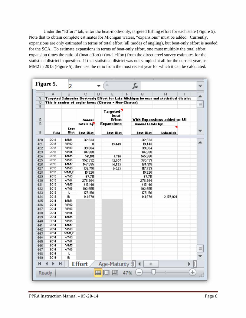
Under the “Effort” tab, enter the boat-mode-only, targeted fishing effort for each state (Figure 5).

Note that to obtain complete estimates for Michigan waters, “expansions” must be added. Currently,

expansions are only estimated in terms of total effort (all modes of angling), but boat-only effort is needed

for the SCA. To estimate expansions in terms of boat-only effort, one must multiply the total effort

expansion times the ratio of (boat effort) / (total effort) from the direct creel survey estimates for the

statistical district in question. If that statistical district was not sampled at all for the current year, as

MM2 in 2013 (Figure 5), then use the ratio from the most recent year for which it can be calculated.


Figure 6.

Figure 7.

Under the “Age-Maturity” tab, enter the total numbers of all Chinook by age, the numbers of

immature Chinook by age, and the numbers of mature Chinook by age (Figure 6). The spreadsheet uses

these numbers to calculate the proportion mature by age and the overall proportion by age (Figure 7).

These proportions are input to the SCA. Since 1986, these data have been provided by MIDNR from

their creel bio-data files. However, data from other states could be added if available, but make sure the

criteria for identifying immature and mature fish are consistent.


Figure 8.

Alewife SCA – Indices of abundance from three sources are used to estimate alewife abundance:

trawl surveys, hydroacoustic surveys, and predator consumption estimates. The USGS Great Lakes

Science Center in Ann Arbor, MI conducts the trawl and hydroacoustic surveys. The consumption

estimates for Chinook salmon are part of the output of the Chinook SCA. This means that the Chinook

SCA must be completed before the alewife SCA. The “Alewife SCA data” spreadsheet should be used to

help organize the data needed. It is located in the “ALE Model Input” folder (Figure 8).


Figure 9.

Figure 10.

Under the “Salmonid Stocking” tab, update the number of salmon and trout stocked in the current

year (Figure 9).

Under the “ALE Proportion by age” tab, update the proportion by age of alewives collected in the

trawl survey (Figure 10).


Figure 11.

Figure 12.

Under the “ALE Trawl Abundance” tab, update the abundances from the trawl survey (Figure

11).

Under the “ALE Acoustic Abundance” tab, update the abundances from the hydroacoustic survey

(Figure 12).


Figure 13.

B. Data for auxiliary indicators – Six auxiliary indicators are included in the analysis: 1) body

condition of Chinook salmon collected from the fishery during July 1 through August 15; 2) charter

fishery catch-per-effort (CPE); 3) average weights of age-3+ female Chinook salmon collected at weirs

and harbors; 4) percent composition of salmonine species in the harvest; 5) relative success in achieving

Fish Community Objectives; and 6) age structure of the alewife population. Data for each are located in

the “Auxiliary Indicators” folder (Figure 1).

Chinook body condition indicator – The body condition of Chinook salmon in mid-summer of

each year is the first auxiliary indicator. Condition is represented as the predicted weight of a 35-inch fish

from a regression of the natural logs of weight (Y) versus length (X). Only fish collected from a

relatively short period during summer (July 1 to August 15) are used to calculate the regression. Length-

weight data are organized by individual state or agency. For example, lengths and weights from the

Illinois creel survey are entered in file “CHS L-W data IL”, lengths and weights from Michigan are

entered in file “CHS L-W data-MI”, and so on. Send spreadsheets to the appropriate agency

representative and ask them to enter the individual lengths and weights of fish in their respective

spreadsheets. For example, Figure 13 is the spreadsheet for Illinois. The units of measure used in the

length-weight regressions are inches and pounds, so unit conversions might be necessary as in Figure 13.


Figure 14.

Chinook catch per effort indicator – The catch per effort (CPE) of Chinook salmon in the charter

fishery for each year is the second auxiliary indicator. Catch per effort is represented as (number of

Chinook salmon harvested) / (targeted, boat-only salmonine effort in angler hours). Catch-per-effort data

files are organized by state. For example, data from Illinois is in file “Charter CPE for CHS - IL”, data

from Michigan is in file “Charter CPE for CHS - MI”, and so on. Send spreadsheets to the appropriate

agency representative and ask them to enter effort and catch in their respective spreadsheets. For

example, Figure 14 is the spreadsheet for Illinois.


Figure 15.

Female Chinook weights at weirs indicator – The average weight of age-3+ female Chinook

salmon collected each year at weirs and harbors is the third auxiliary indicator. Note that these should be

weights of “egg full” fish. Do not include weights of spent fish. Weights of individual females sampled

are organized by state. For example, data from Illinois is in file “Weights of Age 3+ CHS at IL Harbors”.

Send spreadsheets to the appropriate agency representative and ask them to enter the ages and weights in

their respective spreadsheets. For example, Figure 15 is the spreadsheet for Illinois.


Figure 16.

Salmonine harvest composition indicator – The composition of the recreational salmonine harvest

each year is the fourth auxiliary indicator. Composition is represented as the percent by weight of

Chinook salmon, lake trout, steelhead, coho salmon, and brown trout. These same data are already being

organized on a lake-wide basis in the “Extractions Database” so it should be requested from the person in

charge of updating that database (currently Brian Breidert, INDNR).

FCO performance indicator – A measure of the performance of the stocking policy in achieving

the Salmonine Fish Community Objectives (FCO) (Eschenroder et al. 1995) is the fifth auxiliary

indicator. The only data required by this indicator are the annual numbers of salmonines stocked and

these data have already been assembled for the alewife SCA as described above (Figure 9).

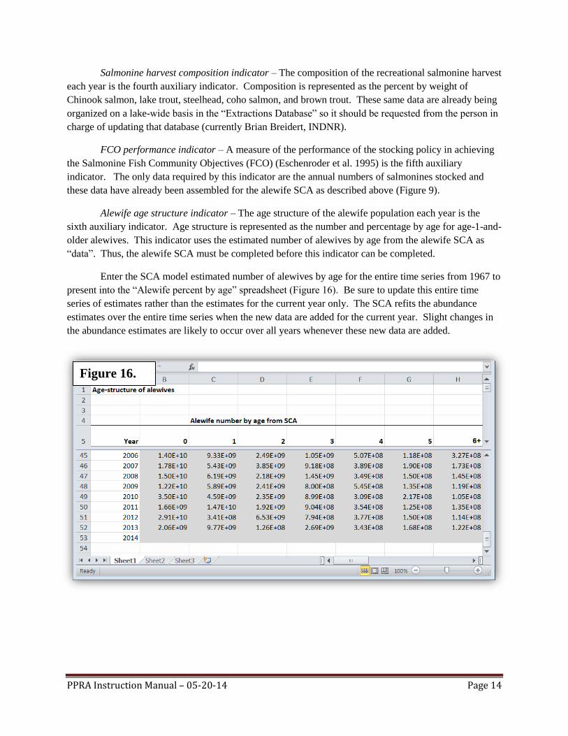
Alewife age structure indicator – The age structure of the alewife population each year is the

sixth auxiliary indicator. Age structure is represented as the number and percentage by age for age-1-and-

older alewives. This indicator uses the estimated number of alewives by age from the alewife SCA as

“data”. Thus, the alewife SCA must be completed before this indicator can be completed.

Enter the SCA model estimated number of alewives by age for the entire time series from 1967 to

present into the “Alewife percent by age” spreadsheet (Figure 16). Be sure to update this entire time

series of estimates rather than the estimates for the current year only. The SCA refits the abundance

estimates over the entire time series when the new data are added for the current year. Slight changes in

the abundance estimates are likely to occur over all years whenever these new data are added.


Figure 17.

Step 2 – Estimate current-year values for biological indicators and update time series of historical

values

A. P-P ratio indicator –

Chinook salmon – Estimate the abundance by age of Chinook salmon using the SCA that is set up

in the “CHS Model” folder. Transfer data from the “Chinook SCA data” spreadsheet into the ADMB

input data file, which is located in the “Chinook Model” folder (Figure 17). This transfer is not set up to

be a simple copy-paste operation. Data must be entered manually.


Figure 18.

The ADMB .dat file is designed to be self-explanatory with text headers and/or notes followed by

each category of data. Figure 18 illustrates the first few data arrays in the “chs_sca” data file.


Figure 20.

Figure 19.

When the data file is updated, double click on the “ADMB Source Code” file (Figure 19) to run

the SCA. ADMB will generate several new files in the “CHS Model” folder. The estimates of the

abundance of Chinook salmon by age will be in the “ADMB Report” file (Figures 19). This output array

is designated as “N” in the report file (Figure 20).


Figure 21.

Find and open the “CHS-ALE Ratio” spreadsheet. It is located in the “CHS-ALE Ratio

Analysis” folder (Figure 19). Copy the Chinook abundance estimates from the ADMB report file and

paste them into the “CHS-ALE Ratio” spreadsheet under the “Chinook Biomass” tab (Figure 21). Be

sure to update the entire time series, and all age classes.


Figure 22.

Update the projection model which predicts the abundance of Chinook salmon for the next 6

years (2014-2019 in Figure 22). Anyone familiar with MS-Excel should be able to understand the logic

behind the projection model by examining the formulas in this spreadsheet. For future survival rates, use

the average survival rate for the last 3 years for each age group. For future numbers of wild smolts, use

the average number for the last 3 years. For future numbers of stocked smolts, use the anticipated number

to be stocked for the current stocking policy.


0

2

4

6

8

10

12

14

16

1960 1970 1980 1990 2000 2010 2020

We

igh

t (M

illio

n k

gs)

Year

Total Biomass of Chinook (Ages 1+) Data Through 2013

SCAA Estimate Projection

Figure 23.

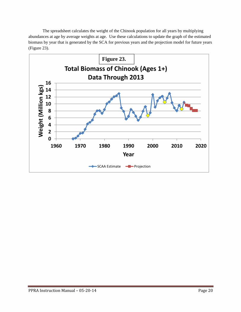
The spreadsheet calculates the weight of the Chinook population for all years by multiplying

abundances at age by average weights at age. Use these calculations to update the graph of the estimated

biomass by year that is generated by the SCA for previous years and the projection model for future years

(Figure 23).


0100200300400500600700800

1960 1970 1980 1990 2000 2010 2020

We

igh

t (M

illio

n k

gs)

Year

Total Biomass of Alewives (Ages 1+) Data Through 2013

Historical Projection Lower Limit Mean

Figure 24.

Alewives – Follow the same procedure for estimating alewife biomass as was used for Chinook

salmon: 1) estimate abundance up to the current year with the alewife SCA using ADMB; 2) estimate

total biomass up to the current year using the spreadsheet; 3) estimate total abundance and biomass for

future years using the projection model, and 4) update the graph of biomass by year (Figure 24). The

ADMB data file and source code are located in the “ALE Model” folder (Figure 17). The alewife

biomass calculations, projection model estimates, and graphic displays are performed in the “CHS-ALE

Ratio” spreadsheet file under the “Alewife Biomass” tab (Figure 21).

The projection model for alewives assumes that adult alewife mortality in the future will change

in proportion to Chinook salmon biomass. The average alewife mortality for the previous 3 years is used

as the initial value, and then it is adjusted up or down based on the projected change in Chinook salmon

biomass. For example, if Chinook salmon biomass is projected to increase by 10%, then alewife

mortality will be adjusted upward by 10%. These calculations are built into the spreadsheet.

For future numbers of age-0 alewife recruits in the projection model, use the average number for

the entire time series as estimated by the SCA.

Figure 24 shows the final results of these procedures. Also, shown is the lower limit and mean

(or target) for alewife biomass. The lower limit of 100 kt was identified by biologists and stakeholders

using structured decision analysis (Jones et al 2008). They decided that alewife biomass below this level

presented an unacceptable risk of population collapse. The target of 240 kt is the mean alewife biomass

from 100 runs of the risk assessment model (Szalai 2003) as was used in that analysis to simulate a 50%

cut in the stocking rate of Chinook salmon, which is the current stocking policy. The lower limit and

target do not change every year, but are used to help judge the success of the stocking policy. For

example, if either the observed or projected alewife biomass is below the lower limit, the stocking policy

should be reviewed.


Figure 25.

0.00

0.02

0.04

0.06

0.08

0.10

0.12

0.14

1960 1970 1980 1990 2000 2010 2020

Rat

io

Year

Predator-Prey Ratio - Chinook (Age 1+)/Alewives (Age 1+) Data Through 2013

Historical Projection Target Upper Limit

Figure 26.

Finally, calculate the P-P ratio for all years in the “CHS-ALE Ratio” spreadsheet under the

“Predator-Prey Ratio” tab (Figure 25) and update the graph showing the estimated ratios over time

(Figure 26).

.


Figure 27.

The target and upper limit for the P-P ratio of 0.050 and 0.100, respectively, were recommended

by SWG (Lake Michigan Salmonid Working Group and Collaborators 2014; Jones et al. 2014). We will

not go into great detail here about how these values were derived, but they were based on runs of the risk

assessment model (Szalai 2003) and comparisons of P-P ratios for similar systems in other lakes.

Basically, these are the P-P ratios corresponding to the target and lower limit defined for the alewife

biomass in Figure 24. Outcomes of the risk assessment model suggest that exceeding a P-P ratio of

0.100, gives the same probability of predator-prey system collapse (15%) as the alewife population falling

below 100 kts.

In addition, comparisons of P-P ratios in other lakes seem to support an upper limit near 0.100.

The Chinook salmon-alewife P-P ratio in Lake Ontario was well below 0.100, at 0.065 from 1999 to 2005

(based on biomass estimates of Murry et al 2009), and while some concern has been expressed about the

sustainability of that predator-prey system, it did not collapse. On the other hand, the Chinook salmon-

alewife predator-prey system of Lake Huron did collapse in 2003-2006 (Johnson et al. 2010), and the

average P-P ratio for the five years prior to the collapse was 0.112 (James Bence, QFC, Michigan State

University, personal communication). Thus, it would seem prudent for managers to avoid P-P ratios near

or above 0.100 in Lake Michigan.

B. Auxiliary Indicators –

Chinook body condition indicator – Use the data analysis feature of MS-Excel to calculate linear

regressions for the current year from the ln-transformed length-weight data supplied by each agency.

Then, accumulate the results for all the agencies in the spreadsheet named “Aux 1 - Trends in Chinook

Condition”, which is located in the “Aux 1 – Analysis” folder. The spreadsheet has a tab for each agency.

Enter the intercepts, slopes, residual mean square (MS), and sample sizes for the regressions for each

agency as shown for the State of Illinois in Figure 27. Then, copy down the regression formula in column

E to estimate the weight of the standard 35-inch Chinook salmon for the current year. This formula uses

the residual MS to correct the bias in the ln-transformed error term as described in Newman (1993).


8.0

10.0

12.0

14.0

16.0

18.0

20.0

22.0

1980 1985 1990 1995 2000 2005 2010 2015

We

igh

t o

f 3

5-i

nch

Ch

ino

ok

(p

ou

nd

s)

Year

Lake Michigan - States Combined Weight of Standard 35-inch Chinook

Lake Michigan Lake Huron

Figure 28.

8

10

12

14

16

18

20

22

1980 1985 1990 1995 2000 2005 2010 2015We

igh

t o

f 3

5-i

nch

Ch

ino

ok

(p

ou

nd

s)

Year

Lake Michigan States Compared to Lake Huron Weight of Standard 35-inch Chinook

Indiana Illinois Michigan

Wisconsin Lake Huron, MI

Figure 29.

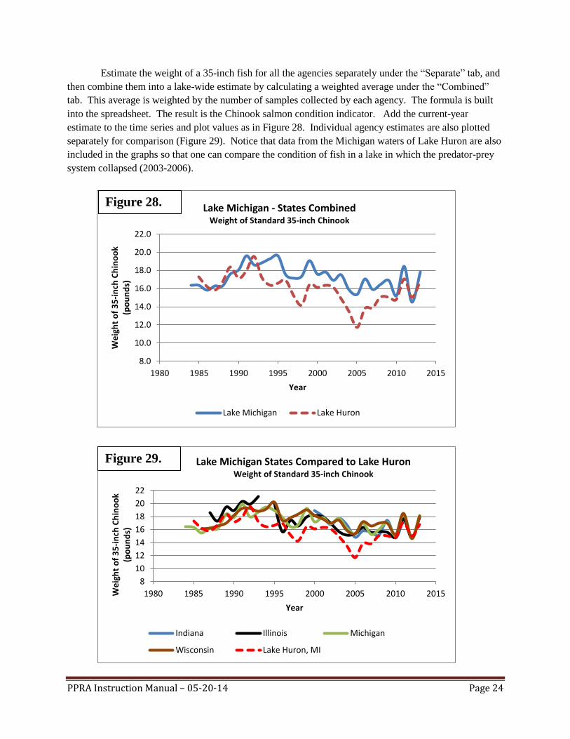
Estimate the weight of a 35-inch fish for all the agencies separately under the “Separate” tab, and

then combine them into a lake-wide estimate by calculating a weighted average under the “Combined”

tab. This average is weighted by the number of samples collected by each agency. The formula is built

into the spreadsheet. The result is the Chinook salmon condition indicator. Add the current-year

estimate to the time series and plot values as in Figure 28. Individual agency estimates are also plotted

separately for comparison (Figure 29). Notice that data from the Michigan waters of Lake Huron are also

included in the graphs so that one can compare the condition of fish in a lake in which the predator-prey

system collapsed (2003-2006).


Figure 30.

Chinook catch per effort indicator – Accumulate the charter catch and effort data from the

individual states in the spreadsheet named “Aux 2 – Charter CPE for CHS”, which is located in the “Aux

2 – Analysis” folder. The spreadsheet has a tab for each agency. Enter the number harvested and

targeted effort for each agency as shown for the State of Illinois in Figure 30. Then, copy down the

formula in column D to estimate the CPE of Chinook salmon for the current year.


0.00

0.05

0.10

0.15

0.20

0.25

0.30

0.35

0.40

1985 1990 1995 2000 2005 2010 2015

Cat

ch p

er H

ou

r

Year

Targeted, Boat Fishing Catch per Hour of Chinook in Lake Michigan Charter Fishery - States Combined

0.00

0.05

0.10

0.15

0.20

0.25

0.30

0.35

0.40

0.45

1970 1980 1990 2000 2010 2020

Cat

ch p

er H

ou

r

Year

Targeted, Boat Fishing Catch per Hour of Chinook in Lake Michigan Charter Fishery - States Separately

Indiana Illinois Michigan Wisconsin

Figure 31.

Figure 32.

Estimate the Chinook salmon CPE for all the agencies separately under the “Separate” tab, and

then combine them into a lake-wide estimate by calculating the 4-state average under the “Combined”

tab. This lake-wide estimate is the sum of the harvests divided by the sum of the efforts. The formula is

built into the spreadsheet. The result is the charter CPE indicator. Add the current-year estimate to the

time series and plot values as in Figure 31. Individual agency estimates of Charter CPE are also plotted

separately for comparison (Figure 32).


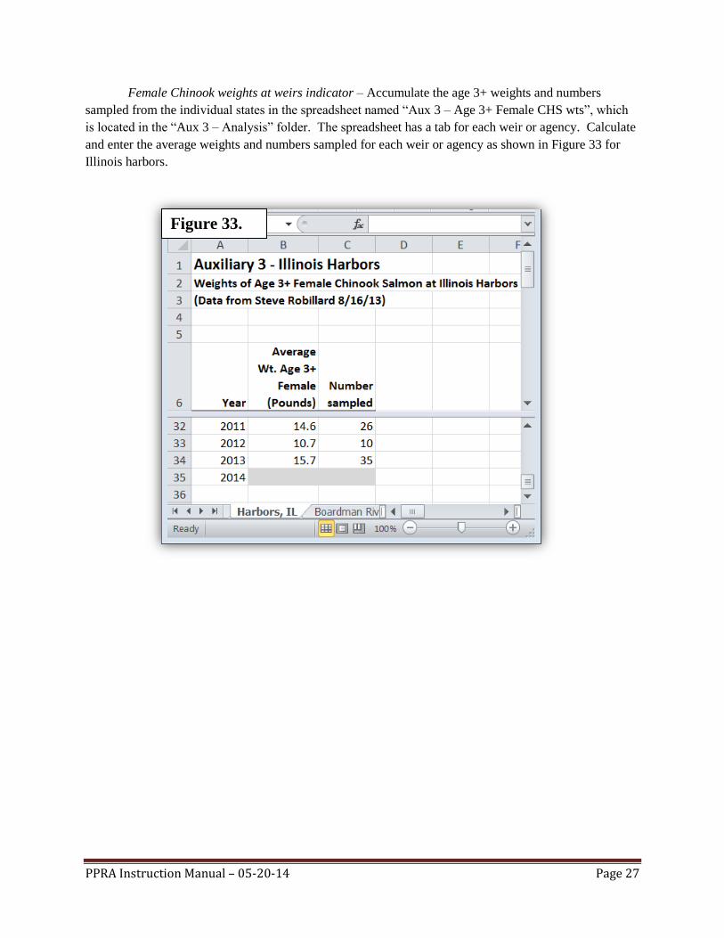
Figure 33.

Female Chinook weights at weirs indicator – Accumulate the age 3+ weights and numbers

sampled from the individual states in the spreadsheet named “Aux 3 – Age 3+ Female CHS wts”, which

is located in the “Aux 3 – Analysis” folder. The spreadsheet has a tab for each weir or agency. Calculate

and enter the average weights and numbers sampled for each weir or agency as shown in Figure 33 for

Illinois harbors.


6.0

8.0

10.0

12.0

14.0

16.0

18.0

20.0

22.0

24.0

1985 1990 1995 2000 2005 2010 2015

Ave

rage

Wei

ght

(Po

un

ds)

Year

Lake Michigan Weirs & Harbors Combined Average Weight of Age-3+ Female Chinook

6

8

10

12

14

16

18

20

22

24

1985 1990 1995 2000 2005 2010 2015

Ave

rage

Wei

ght

(Po

un

ds)

Year

Lake Michigan Weirs & Harbors - Separately Average Weight of Age-3+ Female Chinook

IL Harbors Boardman, MI Little Manistee, MI

Medusa, MI Strawberry, WI

Figure 34.

Figure 35.

Calculate and assemble the average weights of age 3+ females for all the agencies separately

under the “Separate” tab, and then combine them into a lake-wide estimate by calculating a weighted

average under the “Combined” tab. This average is weighted by the number of samples by individual

weir or harbor. The formula is built into the spreadsheet. This result is the female-weight indicator.

Add the current-year estimate to the time series and plot values as in Figure 34. Individual weir or agency

estimates of age-3+ female weights are also plotted separately for comparison (Figure 35).


0.0%

10.0%

20.0%

30.0%

40.0%

50.0%

60.0%

70.0%

80.0%

90.0%

100.0%

1986 1988 1990 1992 1994 1996 1998 2000 2002 2004 2006 2008 2010 2012

Year

Percent of Harvest in Weight for Salmonines

Chinook salmon Coho salmon Lake trout Steelhead Brown trout

Figure 36.

Salmonine harvest composition indicator – Enter the weights harvested for each salmonine

species for the current year in the spreadsheet named “Aux 4 – Harvest Composition - Analysis”, which is

located in the “Aux 4 – Analysis” folder. Plot the time series as a stacked area plot, as shown in Figure

36.


Figure 37.

FCO performance indicator – This indicator is expressed as the “FCO Index”, which is

calculated as the sum of the deviations between the salmonine yields from a hypothetical run of the

CONNECT model (Rutherford 1997, Lake Michigan Salmonid Stocking Task Group 1998) to the yield

expectations identified in the Fish Community Objectives. The hypothetical model run estimates the

yields that would have occurred today if the levels of recreational fishing effort during the 1980s had

continued to present. In reality, fishing effort has declined, which is why these yield predictions are

considered hypothetical. Clark (2012) gives a more detailed description of the “FCO Index” and the

reasoning behind it in Recommendation 3 of his report.

To calculate the “FCO Index”, enter the number of Chinook salmon recruits expected (stocked

and wild) for the current and future years into the “Connect 4” model spreadsheet (Figure 37). This

spreadsheet is located in the “Aux 5 – Data and Model” folder. Enter the same data for each of the other

salmonines under the appropriate spreadsheet tabs. The “CONNECT 4” spreadsheet uses this recruitment

data to estimate potential yields for each species in age-structured models.


Figure 38.

-8000

-6000

-4000

-2000

0

2000

4000

6000

Su

m o

f D

evia

tio

ns

Year

FCO Index

Next, open the spreadsheet named “Aux 5 – FCO Analysis”, which is located in the “Aux 5 –

FCO Analysis” folder. This spreadsheet is linked to the “Connect 4” model spreadsheet, so click “yes” to

update the links when opening the file. The yield estimates will be transferred to appropriate cells under

the “Tables” tab and the deviations between the potential yields and the FCO expectations will be

calculated in column “D” for Chinook salmon, “I” for lake trout, and so on (Figure 38).

The spreadsheet also plots the FCO Index over time (Figure 39). An index value of zero means

that the deviations between the model-predicted and FCO-expected yields sum to zero, which suggests

that the stocking policy in place is coming close to achieving the FCO-expected yields. However, a zero

value could also occur when the “over stocking” of one species equals the “understocking” of another.

Figure 39.


0

2000

4000

6000

8000

10000

12000

Yie

ld

(1000s o

f P

ou

nd

s)

Year

Potential versus FCO Expected Yield for Chinook Salmon

0

500

1000

1500

2000

2500

3000

Yie

ld

(10

00

s p

ou

nd

s)

Year

Potential versus FCO Expected Yield for Lake Trout

0

200

400

600

800

1000

1200

1400

Yie

ld

(10

00

s p

ou

nd

s)

Year

Potential versus FCO Expected Yield for Steelhead

0

500

1000

1500

2000

2500

Yie

ld

(1

00

0s

po

un

ds

)

Year

Potential versus FCO Expected Yield for Coho Salmon

0

200

400

600

800

1000

1200

Yie

ld

(1

00

0s

po

un

ds

)

Year

Potential versus FCO Expected Yield for Brown Trout

One can examine the yield values for each individual species to determine if they exceed or fall

short of their individual FCO expected values. The spreadsheet plots the model-predicted potential yields

and the FCO yield expectations for each species so they can be compared (Figure 40). For example, the

CONNECT model predicted that the stocking rates in place for Chinook salmon and lake trout should

provide potential yields that are fairly close to FCO expectations. However, steelhead and brown trout

stocking rates are predicted to provide yields higher than FCO expectations and coho salmon lower.

Potential Yield FCO Expected Yield

Figure 40.


-

2,000

4,000

6,000

8,000

10,000

12,000

1 2 3 4 5 6+

Nu

mb

er

(Mill

ion

s)

Age

Alewife Numbers by Age Current Year (2013) versus 2001-2005 Average

2001-2005 2013

Alewife age structure indicator – Update the graph comparing the current year alewife population

structure to that of the 2001-2005 average (Figure 41).

Step 3 – Use results to judge the performance of the stocking policy

A. P-P ratio indicator – The idea behind the Chinook salmon-alewife P-P ratio is that it should

be a good measure of trophic balance and that it can be used as a guide for managers to establish and

monitor sustainable stocking rates for Chinook salmon. If desired, the deviations between the target and

projected ratios (Figure 26) can be used to “fine tune” stocking rates by making small changes to

minimize the deviations. The upper limit ratio (Figure 26) can be used as a management “red flag”

trigger. If either the estimated historical or projected ratios exceed the upper limit, it indicates a serous

imbalance could be occurring now or developing in the near future. Such an outcome should generate

immediate and serious discussion regarding reductions in stocking rates.

We conducted a retrospective analysis of the years in which stocking was reduced (1998, 2005,

and 2011) to determine if the PPRA, if it had been available in those years, would have supported the

previous decisions to reduce stocking rates of Chinook salmon. Results showed that the PPRA would

have supported the decisions in every case. The most important finding was that the estimated P-P ratio

for the current year of analysis was always within an acceptable range, but that projections of P-P ratios

for the near future were predicted to exceed the upper limit of 0.100. For example, Figure 42 shows the

results for 2005. The results of the retrospective analysis demonstrate the value of the projection model.

Figure 41.


0.00

0.02

0.04

0.06

0.08

0.10

0.12

0.14

1960 1970 1980 1990 2000 2010 2020

Rat

io

Year

Predator-Prey Ratio - Chinook (Ages 1+)/Alewives (Ages 1+) 2005 Perspective - Status Quo Stocking Rate

Figure 42.

Based on the results of the PPRA through 2013, it appears that the current stocking rate of 1.76

million Chinook salmon smolts is expected to perform well (Figure 26). Of course, this assumes that

rates of recruitment, growth, and mortality of predator and prey remain similar to those occurring in

recent history. Only continued monitoring of these rates can detect unforeseen changes. For example,

recent surveys have suggested that a resurgence of lake trout reproduction could be occurring. If so,

additional wild lake trout would likely increase the predation mortality rate on alewives, and it would be

necessary to account for this in the analysis.

B. Auxiliary Indicators – Results of the auxiliary indicators should be used to supplement the P-

P ratio. For example, if the P-P ratio exceeds the upper limit, calling for serious review of the stocking

policy, the auxiliary indictors can be used to help assess the accuracy and reasonableness of that P-P ratio

estimate. In addition, several of the auxiliary indicators, such as the average weights of females at weirs

and harbors, are direct field measurements in support of the modeling work. Such estimates can be very

useful to help explain the status of the predator-prey system and the reasons for stocking decision to

stakeholders and the general public. Also, the plots of the historical time series for these indicators help

put the current values into context.

Chinook body condition indicator – The relationship between the relative Chinook condition

(predicted weight of a 35-inch fish) and the P-P ratio should help biologists evaluate the validity of the

estimated P-P ratio for a given year. This is especially true when the P-P ratio estimate approaches the

upper limit of 0.100 and suggests management action should be considered.


12.0

13.0

14.0

15.0

16.0

17.0

18.0

19.0

20.0

0.000 0.020 0.040 0.060 0.080 0.100

We

igh

t o

f 3

5-i

nch

Re

fere

nce

Fis

h

Predator-Prey Ratio

Chinook Condition versus Predator-Prey Ratio Figure 43.

The weight of predators at a given length should increase as the number of prey per predator

(potential ration size) increases. Therefore, the relative condition of predators should be inversely related

to the P-P ratio. A plot of Chinook condition versus P-P ratio supports this idea (Figure 43). Also, a

regression of Chinook condition versus P-P ratio (solid line in Figure 43) is statistically significant (R2 =

0.57, P < 0.01). Judging from this regression line in Figure 43, when P-P ratios approach the upper limit

of 0.100, the predicted weight of a standard 35-inch fish should decline to about 14 pounds. If not, then

the estimate of the P-P ratio might be incorrect.

Chinook condition estimates in Lake Huron also support the idea that predator-prey situations

leading to predicted weights of 14 pounds for 35-inch fish should be avoided (Figure 28). Predicted

weights were below 14 pounds for 4 consecutive years (2004-2007) in Lake Huron.

The problem with the Chinook condition indicator is that by the time the predicted weights reach

14 pounds, it might be too late for managers to take action to prevent a collapse as illustrated by the

timing of events in Lake Huron. Alewife populations collapsed in 2003 when the predicted condition of

Chinook salmon was 14.9 pounds, a value that had occurred and been approached several times in the

past with no apparent problem (Figure 28). It was not until 2004, after the alewife population had already

collapsed, that predicted weights dropped to 13.5 pounds and lower (Figure 28). Hopefully, the P-P ratio

projection model for Lake Michigan can do a better job of giving advanced warning of these serious

problems.

Chinook catch per effort indicator – The catch per hour from the charter fishery is monitored to

help judge the relative performance of the fishery from year to year. From the perspective of anglers

catch per hour is one of the most important and noticeable performance measures, so anglers usually have

a strong interest in the results of this indicator. Although, interpreting and communicating the

significance of a given catch rate can be challenging. While high catch rates give anglers the impression

that fishing is very good, high catch rates usually occur in years with high P-P ratios and could indicate a


0.00

0.05

0.10

0.15

0.20

0.25

0.30

0.35

0.40

0.000 0.020 0.040 0.060 0.080 0.100

Cat

ch p

er

Ho

ur

of

Ch

ino

ok

sal

mo

n

Predator-Prey Ratio

Charter Boat CPE versus Predator-Prey Ratio Figure 44.

8.0

10.0

12.0

14.0

16.0

18.0

20.0

22.0

13.0 14.0 15.0 16.0 17.0 18.0 19.0 20.0 21.0

Ave

rage

We

igh

t o

f A

ge 3

+

Weight of 35-in Reference Fish in creel

Average Weight of age-3+ Female at Wiers and Harbors versus Predicted Weight of 35-inch Fish in Creel

Figure 45.

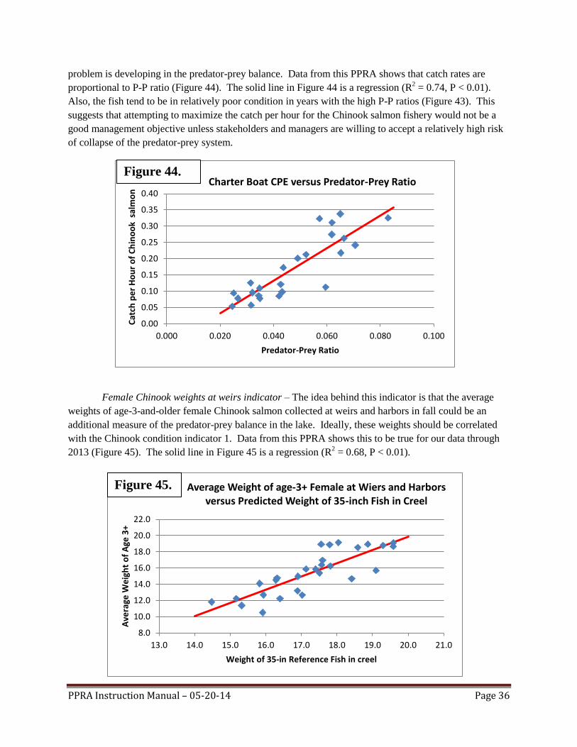
problem is developing in the predator-prey balance. Data from this PPRA shows that catch rates are

proportional to P-P ratio (Figure 44). The solid line in Figure 44 is a regression (R2 = 0.74, P < 0.01).

Also, the fish tend to be in relatively poor condition in years with the high P-P ratios (Figure 43). This

suggests that attempting to maximize the catch per hour for the Chinook salmon fishery would not be a

good management objective unless stakeholders and managers are willing to accept a relatively high risk

of collapse of the predator-prey system.

Female Chinook weights at weirs indicator – The idea behind this indicator is that the average

weights of age-3-and-older female Chinook salmon collected at weirs and harbors in fall could be an

additional measure of the predator-prey balance in the lake. Ideally, these weights should be correlated

with the Chinook condition indicator 1. Data from this PPRA shows this to be true for our data through

2013 (Figure 45). The solid line in Figure 45 is a regression (R2 = 0.68, P < 0.01).


Salmonine harvest composition indicator – Establishing a diverse salmonine community is part of

the fish community objectives for Lake Michigan (Eshenroder et al. 1995). The composition in weight of

the salmonine harvest has been estimated for many years as one measure of that diversity. The estimate

was added to the PPRA to help provide a more complete representation of the salmonine community.

FCO performance indicator – This indicator was added to the PPRA to help judge how

successful management practices have been in achieving the yield expectations set forth in the Salmonine

Objectives (Eshenroder et al. 1995). The FCO index is one way to measure and communicate the overall

performance of the stocking policy and the hypothetical yields from the CONNECT model add species-

by-species performance measures.

Alewife age structure indicator – The idea behind this indicator was that the effects of excessive

predation on alewives might be revealed by erosion of the number of age groups in the population and/or

a reduction in the absolute numbers of older fish. In addition, this indicator could help monitor natural

fluctuations in year-class strength of alewives. One way to analyze the age structure would be to

compare the numbers by age of alewives for the current year to that of a standard population deemed to

have an ideal age structure. For example, the average 2001-2005 population age structure could be used

as a standard for comparison because the alewife biomasses (Figure 24) and the P-P ratios (Figure 26)

were near target levels in those years. Thus, it seems reasonable to assume that the age structure in these

years was close to ideal. Notice that average numbers by age in 2001-2005 were fairly evenly distributed,

and included 670,000 fish (5.5%) age 6 or older (Figure 41). On the other hand, numbers by age in 2013

were unevenly distributed, and included only 122,000 fish (0.9%) age 6 or older.

Overall, 94% of the total abundance of alewives in 2013 was within only two age groups (1 and

3). Managers should consider such a skewed age structure as a precarious situation for the alewife

population. Thus, the alewife age structure in 2013 should be considered as additional evidence that

cutting Chinook salmon stocking in 2013 was a good decision.


References

Clark, R. D., Jr. 2012. Review of Lake Michigan Red Flags Analysis. Quantitative Fisheries Center

Technical Report 2012-01, Michigan State University, East Lansing, MI.

Jones, M., R. Clark, and I. Tsehaye. 2014. Workshops to revise and improve the Lake Michigan red

flags analysis. Science Transfer Project Completion Report. Great Lakes Fisheries Commission.

Ann Arbor, MI.

Eshenroder, R. L., M. E. Holey, T. K. Gorenflo, and R. D. Clark, Jr. 1995. Fish Community Objectives

for Lake Michigan. Great Lakes Fishery Commission Special Publication 95-3, Ann Arbor,

Michigan.

Fournier, D.A., H.J. Skaug, J. Ancheta, J. Ianelli, A. Magnusson, M.N. Maunder, A. Nielsen, and J.

Sibert. 2012. AD Model Builder: using automatic differentiation for statistical inference of highly

parameterized complex nonlinear models. Optim. Methods Softw. 27:233-249.

Johnson, J. E., S. P. DeWitt, and D. J. A. Gonder. 2010. Mass marking reveals emerging self regulation

of the Chinook salmon population in Lake Huron. North American Journal of Fisheries

Management 30: 518-529.

Jones, M. J., J. R. Bence, E. B. Szalai, and Wenjing Dai. 2008. Assessing stocking policies for Lake

Michigan salmonine fisheries using decision analysis. In: D. F. Clapp and W. Horns, editors. The

State of Lake Michigan in 2005. Great Lakes Fishery Commission Special Publication 08-02. pp

81-88.

Lake Michigan Salmonine Stocking Task Group. 1998. Final Report to the Great Lakes Fishery

Commission, Lake Michigan Technical Committee. 26 pp.

Lake Michigan Salmonid Working Group and Collaborators. 2014. A summary of review efforts for the

Lake Michigan Red Flags Analysis and proposed recommendations for the Predator-Prey Ratio.

Report to the Great Lakes Fishery Commission, Lake Michigan Committee in Windsor, Ontario,

March 26, 2014.

Murry, B. A., M. J. Connerton, R. O’Gorman, D. J. Stewart, and N. H. Ringlery. 2009.

Lakewide estimates of alewife biomass and Chinook salmon abundance and consumption

in Lake Ontario, 1989-2005: Implications for prey fish sustainability. Transactions of the

American Fisheries Society 139(1):223-240.

Newman, M. C. 1993. Regression analysis of log-transformed data: statistical bias and its

correction. Environmental Toxicology and Chemistry 12: 1129-1133.

Rutherford, E. R., 1997. Evaluation of natural reproduction, stocking rates, and fishing regulations for

steelhead, Chinook salmon, brown trout, and coho salmon in Lake Michigan. Michigan

Department of Natural Resources. Federal Aid to Fish Restoration Final Report. F-35-R-22.

Study 650. Ann Arbor.


Szalai, E. B. 2003. Uncertainty in the population dynamics of alewife (Alosa pseudoharengus) and bloater

(Coregonus hoyi) and its effects on salmonine stocking strategies in Lake Michigan. Ph.D. thesis.

Mich. State Univ., East Lansing, MI.

Tsehaye, I., M. L. Jones, T. O. Brenden, J. R. Bence, and R. M. Claramunt. 2014a. Changes in the

Salmonine community of Lake Michigan and their implications for predator–prey balance.

Transactions of the American Fisheries Society 143:420-437.

Tsehaye, I., M. L. Jones, J. R. Bence, T. O. Brenden, C. P. Madenjian, and D. M. Warner. 2014b. A

multispecies statistical age-structured model to assess predator–prey balance: application to an

intensively managed Lake Michigan pelagic fish community. Canadian Journal of Fisheries and

Aquatic Sciences 71:1-18.

Instruction Manual for the Lake Michigan Chinook Salmon ... · PPRA Instruction Manual – 05-20-14...

Documents

Transcript of Instruction Manual for the Lake Michigan Chinook Salmon ... · PPRA Instruction Manual – 05-20-14...