fulltext.calis.edu.cnfulltext.calis.edu.cn/iop/0305-4470/36/38/301/a33801.pdf · INSTITUTE OF...

INSTITUTE OF PHYSICS PUBLISHING JOURNAL OF PHYSICS A: MATHEMATICAL AND GENERAL

J. Phys. A: Math. Gen. 36 (2003) 9799–9825 PII: S0305-4470(03)64488-4

Symmetry, complexity and multicritical point of thetwo-dimensional spin glass

Jean-Marie Maillard1, Koji Nemoto2 and Hidetoshi Nishimori3

1 LPTHE, Tour 24, 5 eme etage, case 7109, 2 Place Jussieu, 75251 Paris Cedex 05, France2 Division of Physics, Hokkaido University, Sapporo 060-0810, Japan3 Department of Physics, Tokyo Institute of Technology, Oh-okayama, Meguro-ku,Tokyo 152-8551, Japan

Received 6 June 2003Published 10 September 2003Online at stacks.iop.org/JPhysA/36/9799

AbstractWe analyse models of spin glasses on the two-dimensional square lattice byexploiting symmetry arguments. The replicated partition functions of theIsing and related spin glasses are shown to have many remarkable symmetryproperties as functions of the edge Boltzmann factors. It is shown that theapplications of homogeneous and Hadamard inverses to the edge Boltzmannmatrix indicate reduced complexities when the elements of the matrix satisfycertain conditions, suggesting that the system has special simplicities undersuch conditions. Using these duality and symmetry arguments we present aconjecture on the exact location of the multicritical point in the phase diagram.

PACS numbers: 05.50.+q, 75.10.Hk, 75.50.Lk

1. Introduction

Properties of spin glasses are well understood in mean-field models, which show suchanomalous behaviour as replica symmetry breaking, multivalley structure and slow dynamics[1, 2]. The difficult problem of whether or not these mean-field predictions apply to realisticfinite-dimensional systems is still largely unsolved, and active investigations are carried outmainly using numerical methods [2]. Very little systematic analytical work exists, an exceptionbeing a symmetry argument using gauge invariance to derive the exact internal energy andseveral other exact/rigorous relations [3, 4].

In the present paper we develop another type of symmetry argument for models of spinglasses in two dimensions under the replica formalism. Our analyses reveal a variety ofinvariance properties of the replicated partition function under transformations of the edgeBoltzmann factors, a notable example of which is the duality transformation.

Also discussed are complexities of the edge Boltzmann matrix under inversions. It is wellestablished that integrable systems such as the standard scalar Potts model have remarkablyreduced complexities of the edge Boltzmann matrix when the parameters satisfy integrability

0305-4470/03/389799+27$30.00 © 2003 IOP Publishing Ltd Printed in the UK 9799

http://stacks.iop.org/ja/36/9799

9800 J-M Maillard et al

conditions [5]. Analogous (but not the same) behaviour is observed in our present problem,suggesting simplified (if not integrable) properties of the systems in restricted regions in thephase diagram.

The results concerning symmetry properties are used to present a conjecture on the locationof the multicritical point in the phase diagram. Although the argument is not a mathematicallycomplete proof, we expect the prediction to be exact for several reasons including agreementwith numerical results in many different models and satisfaction of inequalities.

It should be remembered that most of the analyses are for real replicas, that is, the numberof replicas is a positive integer. The quenched limit of vanishing number of replicas is discussedin relation only to limited cases including the conjectured location of the multicritical point.

In the next section symmetries of the system are derived. The replicated partition functionis demonstrated to be invariant under several different types of transformations of the edgeBoltzmann factors. It is shown that a special subvariety exists which satisfies remarkableenhanced symmetries. Complexities under applications of matrix inverses are treated insection 3. Here also the same subvariety as above is seen to have reduced complexities,suggesting its special role. A conjecture on the multicritical point is presented in section 4and numerical evidence supporting the conjecture is discussed. The final section is devoted tosummary and discussions.

2. Symmetries of the partition function

In this section we first derive the expression of the replicated partition function in terms ofthe edge Boltzmann factors. Then the symmetries and related properties of the partitionfunction are discussed. The arguments are first developed for the ±J Ising model and then aregeneralized to a broader class of models (such as the Gaussian spin glass and random chiralPotts model) in the last part of this section.

2.1. Replicated partition function

Let us start by considering the Hamiltonian of the ±J Ising model

H = −∑〈ij〉

JijSiSj (1)

where Jij is ferromagnetic J (>0) with probability p and antiferromagnetic −J with 1 − p.The sum extends over nearest neighbours on the square lattice. The randomness in Jij willbe treated by the replica method. We will mainly consider the case of positive integer n,the number of replicas. Some results for the quenched limit n → 0 will be discussed insubsequent sections. The constraints of Ising spins and the ±J distribution of the interactionswill be relaxed later in the present section.

After the average over bond configurations, the system becomes spatially homogeneous4,and the partition function

[Zn]av ≡ Zn (2)

where the square brackets with subscript ‘av’ denote the configurational average, is specifieduniquely by the edge Boltzmann matrix representing neighbouring interactions. For example,when n = 1 (the annealed model), the edge Boltzmann matrix is

p

[w0 w1

w1 w0

]+ (1 − p)

[w1 w0

w0 w1

]≡

[x0 x1

x1 x0

]≡ A1 (3)

4 Except for boundary effects which are irrelevant to thermodynamic properties and will be ignored.

Symmetry, complexity and multicritical point of the two-dimensional spin glass 9801

where w0 = eK,w1 = e−K with K = J/kBT , and x0 denotes the edge Boltzmann factor forparallel configuration of neighbouring spins whereas x1 is for antiparallel spins. Similarly, forn = 2 we have the edge Boltzmann matrix

p

[w0 w1

w1 w0

]⊗

[w0 w1

w1 w0

]+ (1 − p)

[w1 w0

w0 w1

]⊗

[w1 w0

w0 w1

]. (4)

This is a 4 × 4 matrix of hierarchical structure

x0 x1 x1 x2

x1 x0 x2 x1

x1 x2 x0 x1

x2 x1 x1 x0

≡ A2 =

[A1 B1

B1 A1

](5)

with x0 = pw20 + (1 − p)w2

1, x1 = pw0w1 + (1 − p)w1w0 and x2 = pw21 + (1 − p)w2

0. The2 × 2 matrix B1 is obtained from A1 by replacing x0 and x1 with x1 and x2, respectively:B1 = A1(x0 → x1, x1 → x2). The element x0 represents the two parallel spin pairs onneighbouring sites (such as ++ for replica 1 and ++ for replica 2), x1 is for one parallel andone antiparallel pairs (such as ++, +−), and x2 corresponds to two antiparallel pairs (+−,−+for example).

The edge Boltzmann matrix of larger n can be derived by recursions. The general formulais

p

[w0 w1

w1 w0

]⊗n

+ (1 − p)

[w1 w0

w0 w1

]⊗n

≡ An =[An−1 Bn−1

Bn−1 An−1

](6)

where Bn−1 = An−1(xk → xk+1; k = 0, 1, . . . , n − 1). The partition function (2) is a functionof the matrix elements of An,

Zn(x0, x1, . . . , xn). (7)

Here xk denotes the Boltzmann factor of the spin configuration with k antiparallel spin pairsamong n neighbouring pairs.

In the symmetry arguments developed subsequently, we will often consider the case wherethe elements xk are independent of each other although they are originally related through theparameters of the ±J Ising model (K and p) by the relations

x0 = pwn0 + (1 − p)wn

1

x1 = pwn−10 w1 + (1 − p)wn−1

1 w0

x2 = pwn−20 w2

1 + (1 − p)wn−21 w2

0 (8)

...

xn = pwn1 + (1 − p)wn

0 .

An advantage to considering generic points in the space spanned by the elements of the edgeBoltzmann matrix

S = {x = (x0, x1, x2, . . . , xn) | xk ∈ R (k = 0, 1, . . . , n)} (9)

is that we can discuss various well-known models such as the 2n-state standard scalar Pottsmodel which has x1 = x2 = x3 = · · · = xn: all but one (x0) spin configurations have the sameBoltzmann factors. The n-replicated ±J Ising model with the edge Boltzmann factor (8) lieson a two-dimensional submanifold T of S:

T = {x ∈ S | xk = pwn−k

0 wk1 + (1 − p)wn−k

1 wk0 (k = 0, 1, . . . , n)

}(10)


2.2. Duality

Some spin systems in two dimensions have invariance properties under duality transformations.The formulation of duality by Wu and Wang [6] is particularly useful for our problem havingthe edge Boltzmann matrix (6) of hierarchical structure. According to these authors, thedual Boltzmann factors are derived simply by Fourier sums applied to each 2 × 2 block(corresponding to each replica) of the edge Boltzmann matrix (6).5 The simplest case is theannealed model n = 1 of equation (3): its dual Boltzmann factors are the sum and differenceof the original Boltzmann factors with appropriate normalization,

√2x∗

0 = x0 + x1

√2x∗

1 = x0 − x1. (11)

As an example, when the system is purely ferromagnetic p = 1 in equation (3), if we definethe dual coupling K∗ by e−2K∗ = x∗

1/x∗0 (remembering e−2K = x1/x0 = w1/w0), we have

from equation (11) the familiar duality relation of the ferromagnetic Ising model,

e−2K∗ = w0 − w1

w0 + w1= tanh K. (12)

In the case of n = 2 with equations (4) and (5), it is necessary to generate combinations ofsums and differences of appropriate matrix elements to obtain the dual Boltzmann factors,

2x∗0 = (x0 + x1) + (x1 + x2) = x0 + 2x1 + x2

2x∗1 = (x0 − x1) + (x1 − x2) = x0 − x2 (13)

2x∗2 = (x0 − x1) − (x1 − x2) = x0 − 2x1 + x2.

The formula for general n with the edge Boltzmann matrix (6) is

�n = 1

2n

[1 11 −1

]⊗n [An−1 Bn−1

Bn−1 An−1

] [1 11 −1

]⊗n

(14)

where the entries of the diagonal matrix �n are the dual Boltzmann factors 2n/2x∗m in a certain

order. More explicitly, the dual Boltzmann factors, which are linear combinations of theoriginal Boltzmann factors, can be written from equation (14) as

2n/2x∗m =

n∑k=0

Dkmxk (15)

where the Dkm are the coefficients of the expansion of (1 − t)m(1 + t)n−m:

(1 − t)m(1 + t)n−m =n∑

k=0

Dkmtk (16)

that is,

Dkm =

k∑l=0

(−1)l(

m

l

)(n − m

k − l

). (17)

To understand equation (16) we first note that m antiparallel pairs are chosen to generatex∗

m for dual spin pairs, which is reflected in the parameter m on the left-hand side of thisequation. This is equivalent to choosing m of the second rows (1,−1) from the direct productof n 2×2 matrices in equation (14).6 Then we choose k antiparallel pairs of original spins as inequation (17) to obtain the coefficient of xk .5 Fourier sums for the two-component (Ising) case are just the sum and difference of two elements.6 As seen in equation (11), an antiparallel spin pair in the dual space corresponds to the difference (the row (1, −1))of two original Boltzmann factors.


On the square lattice the partition function remains invariant under the dualitytransformation of edge Boltzmann factors [6]:

Zn(x0, x1, x2, . . . , xn) = Zn(x∗0 , x∗

1 , x∗2 , . . . , x∗

n) (x ∈ S) (18)

apart from a trivial factor 2n and boundary effects, both of which are irrelevant tothermodynamic properties and will be ignored in this paper. Note that the symmetry underduality (18) is valid for any values of the edge Boltzmann factors x0, x1, x2, . . . , xn, whichdo not necessarily satisfy the relation (8) of the ±J Ising model as indicated by the symbolx ∈ S at the end of equation (18).

It will be useful to write explicitly the general duality transformation (15) applied to thespecific case of the ±J Ising model for later use, namely, for the case x ∈ T (⊂ S). Again wefirst write the formula for the simple case of n = 2 written in equation (13) so that the readerunderstands the structure:

2x∗0 = p(w0 + w1)

2 + (1 − p)(w1 + w0)2 = (w0 + w1)

2

2x∗1 = p(w0 + w1)(w0 − w1) + (1 − p)(w1 + w0)(w1 − w0)

(19)= (2p − 1)(w0 + w1)(w0 − w1)

2x∗2 = p(w0 − w1)

2 + (1 − p)(w1 − w0)2 = (w0 − w1)

2.

The general formula is

2n/2x∗2m = (w0 + w1)

n−2m(w0 − w1)2m

2n/2x∗2m+1 = (2p − 1)(w0 + w1)

n−2m−1(w0 − w1)2m+1.

(20)

2.3. Symmetries under sign changes of coupling constants

In the present subsection the edge Boltzmann factors are regarded as functions of the parametersof the ±J Ising model following equation (8), x ∈ T . The partition function Zn is invariantunder the change of the sign of coupling constant K → −K at all bonds if the system is onthe square lattice. This change of the sign exchanges w0 and w1, and consequently, accordingto equation (8), xk is exchanged with xn−k:

Zn(x0, x1, x2, . . . , xn) = Zn(xn, xn−1, xn−2, . . . , x0) (x ∈ T ). (21)

Combination of two symmetries, duality (18) and change of sign of K (21), leads to anothersymmetry. On the right-hand side of equation (16) the change of sign of t is equivalent tothe change of the sign of Dk

m for odd k. The left-hand side of equation (16) suggests thatthe change of sign of t is also realized by exchange of m and n − m. Then we conclude inequation (15) that the change of sign of xk for odd k on the right-hand side

Dkmxk → (−1)kDk

mxk (22)

should be performed simultaneously with the exchange of x∗m and x∗

n−m to keep this dualityequation valid. Using duality (18) we therefore find the following symmetry,

Zn(x0,−x1, x2,−x3, . . . , (−1)nxn)

= Zn(x∗n, x∗

n−1, . . . , x∗1 , x∗

0 )

= Zn(x∗0 , x∗

1 , . . . , x∗n−1, x

∗n)

= Zn(x0, x1, . . . , xn) (x ∈ T ). (23)

The second equality comes from equation (21) and the final relation is duality (18).


When the number of replicas is even n = 2q, the partition function has additionalsymmetry which exchanges xk with x2q−k for k odd only:

Z2q(x0, x1, x2, x3, x4, . . . , x2q−3, x2q−2, x2q−1, x2q)

= Z2q(x0, x2q−1, x2, x2q−3, x4, . . . , x3, x2q−2, x1, x2q) (x ∈ T ). (24)

It is convenient to start the proof from the following expression of the edge Boltzmann factorsgeneralizing equation (8),

x0 =∑

l

pl e2qKl

x1 =∑

l

pl e2(q−1)Kl

x2 =∑

l

pl e2(q−2)Kl

... (25)

x2q−2 =∑

l

pl e−2(q−2)Kl

x2q−1 =∑

l

pl e−2(q−1)Kl

x2q =∑

l

pl e−2qKl

where the sum runs over l = 1, 2 with p1 = p, p2 = 1 − p and K1 = K,K2 = −K for the±J Ising model. We would like the xk with k even to remain invariant and the xk with k oddto be changed into x2q−k . As one can see from equation (25), this may be considered to be atransformation K → −K for odd k only:

xk(K) → xk((−1)kK). (26)

The sign (−1)k actually corresponds to the sign of �i�j for neighbouring sites i and j , where�i = σ

(1)i σ

(2)i · · · σ (2q)

i and �j = σ(1)j σ

(2)j · · · σ (2q)

j , because �i�j is 1 for even number ofantiparallel pairs and is −1 otherwise. Formula (25) can be written as

xk =∑

l

pl exp

(Kl

n∑α=1

σ(α)i σ

(α)j

)(27)

where k pairs among 2q pairs of neighbouring spins are antiparallel∑

α σ(α)i σ

(α)j = 2q − 2k.

Changing Kl as

Kl → �i�jKl (28)

amounts to changing the edge Boltzmann factor as follows:

xk →∑

l

pl exp

(Kl�i�j

n∑α=1

σ(α)i σ

(α)j

). (29)

In other words this is equivalent to performing for each replica a non-trivial Mattistransformation depending on all the other replicas:

σ(α)i → τ

(α)i = �iσ

(α)i =

∏β =α

σ(β)

i . (30)


Note that, as far as dummy variables to be summed over are concerned, the τ(α)i are as good

as the σ(α)i : this is a one-to-one change of variables. Actually one goes back from the τ

(α)i to

the σ(α)i by performing the same transformation as that defining the τ

(α)i :

τ(α)i → σ

(α)i =

∏β =α

τ(β)

i =∏β =α

(�iσ

(β)

i

) = �2q−1i �iσ

(α)i . (31)

We have used the identity �2q

i = +1. Therefore this Mattis transformation is an involution,and we have proved equation (26) which is equivalent to the symmetry (24).

Let us point out another interesting symmetry of the partition function which can be derivedfrom a combination of symmetries discussed so far. If we denote the duality transformation(15) symbolically as D and the exchange of xk and x2q−k for even n and odd k in equation (24)as M, the combination

D2 = D · M (32)

also leaves the partition function invariant as long as the system satisfies the conditions for Dand M to be the true symmetry such as the lattice structure (square lattice) and even n. Thisduality-like symmetry under the transformation D2 will be used in the next subsection. It isworth noting here that D and M commute for n even (D · M = M · D), and D,M and D2 areall involutions, D2 = M2 = D2

2 = 1.

2.4. Subvariety and duality

The ±J Ising model with quenched randomness has remarkable properties along a line (curve)in the phase diagram defined by the relation

exp(−2K) = 1 − p

p(33)

known as the Nishimori line (NL) [3, 4]. Similar interesting behaviour is observed on the sameline also in the replicated system with n = 2 [7]. In this subsection we analyse symmetriesof the replicated system with general integer n under the condition (33) using the results ofprevious subsections.

Let us consider the ±J Ising model on the square lattice whose parameters satisfyequation (33). From equations (8) and (33), the latter being equivalent to p = w0/(w0 + w1)

and 1 − p = w1/(w0 + w1), it is straightforward to see that the following relations hold:

x1 = xn x2 = xn−1 x3 = xn−2, . . . , xk = xn−k+1, . . . . (34)

Condition (33) reduces the degree of freedom from two (p and K) to one. This means thatwe restrict ourselves to a one-dimensional curve in the (n + 1)-dimensional space S. It willbe useful to relax this constraint and consider the ([(n + 1)/2] + 1)-dimensional submanifoldof S specified only by equation (34), where [x] stands for the largest integer not exceeding x.We shall call this submanifold the subvariety N :

N = {x ∈ S | xk = xn−k+1 (k = 1, 2, . . . , n)}. (35)

The subvariety N of course includes the one-dimensional curve NL specified by equation (33):NL ⊂ N .

By the duality (15), N is transformed into the dual N ∗ satisfying

x1 = x2 x3 = x4 x5 = x6, . . . , x2m−1 = x2m, . . . . (36)

To prove this fact, we first note that condition (34) implies that the coefficient of xk (= xn−k+1)

on the right-hand side of equation (15) is

Dkm(n) + Dn−k+1

m (n) (37)


where we have written the n-dependence of Dkm explicitly. Then the relation (36) follows if

we can show

Dk2m−1(n) + Dn−k+1

2m−1 (n) = Dk2m(n) + Dn−k+1

2m (n) (38)

the left-hand side of which is the coefficient of xk(=xn−k+1) of 2n/2x∗2m−1 in equation (15) and

the right-hand side is for xk(=xn−k+1) of 2n/2x∗2m. Equation (38) can be proved by induction

with respect to n: the validity for small n(= 1, 2, 3) is checked trivially. Let us assume thatequation (38) is valid for n. Then it is not difficult to show that the same equation holds forn + 1 using the following recursion relation,

Dkm(n + 1) = Dk

m(n) + Dk−1m (n) (39)

which is derived by multiplying both sides of equation (16) by 1 + t (which amounts to thechange n → n + 1). This ends the proof.

Comparison of equations (34) and (36) suggests that the subvariety N is in general notself-dual, N = N ∗. When n is even n = 2q, the partition function has an additional symmetry(24), M in the notation of equation (32). Then the combined transformation D2 = D · M

keeps the subvariety invariant, N = N ∗: the application of D2 to N is shown to yield thesame relation as equation (34)

x∗1 = x∗

2q x∗2 = x∗

2q−1 x∗3 = x∗

2q−2, . . . , x∗m = x∗

2q−m+1, . . . . (40)

The proof is outlined in appendix A. We therefore conclude that the subvariety N is globallyself-dual when n is even, that is, any point in the submanifold defined by equation (34) ismapped by D2 to another point in the same submanifold (but is not fixed point-by-point ingeneral).

2.5. Inversions

The edge Boltzmann matrix An with generic values of the elements (x0, x1, x2, . . . , xn) has theremarkable property that its inverse matrix has the same structure; the inverse matrix has thesame arrangement of elements as the original matrix. To show this we first note that the entriesof the Boltzmann matrix are defined up to a common multiplicative factor, and therefore wecan also discuss, instead of the matrix inversion An → A−1

n , a homogeneous matrix inversiontransformation I (actually a homogeneous polynomial transformation):

An → A−1n · det(An). (41)

Let us also introduce the homogeneous transformation J corresponding to the inversion ofelements of the dual matrix (Hadamard inverse), yk → 1/yk (k = 0, 1, . . . , n),7

J : yk −→m=n∏

m=0,m=k

ym. (42)

At first sight, performing the matrix inversion of the 2n × 2n Boltzmann matrix An mayseem to yield quite large calculations. However, since the duality transformation actuallydiagonalizes matrix An as was mentioned in relation to equation (14), it is straightforward tosee that the matrix inversion just amounts to changing the dual variables x∗

m into their simpleinverse : x∗

m → 1/x∗m. From this remark, it is straightforward to see that the matrix inverse

of An is a 2n × 2n matrix of the same form as the original An (but of course with differentelements : xk → x ′

k). With obvious notation, and since there is no possible confusion, we willalso denote by I this transformation on the xk:

I : xk −→ x ′k. (43)

7 Transformation J is analogous to negating various coupling constants.


Up to a common multiplicative factor one thus has (since D is an involution, that is, D2 = 1)

D · I · D ∝ J or I ∝ D · J · D. (44)

Remark. One should recall that the two involutions I and J are actually (nonlinear)symmetries of the phase diagrams of (anisotropic) spin edge lattice models [5, 8, 9]. Fromequation (44) one sees that these ‘nonlinear’ symmetries of the phase diagrams are closelyrelated to the (linear) duality symmetry. A duality symmetry exists when the edge Boltzmannmatrix corresponds to cyclic matrices or a semi-direct product of cyclic matrices [6]. However,when a duality symmetry does not exist, such as for instance the Ising model in a magnetic field,the two ‘nonlinear’ symmetries I and J still exist and can still be used to analyse the phasediagram [8].

2.6. Spin representation of the dual Boltzmann factor

The elements of the dual edge Boltzmann factors of the replicated ±J Ising model (20) have aninteresting symmetry. It is instructive to take the ratios of x∗

1 , x∗2 , . . . to x∗

0 (which is equivalentto setting the energy level of all-parallel state to 0):

x∗2m−1/x

∗0 = (2p − 1)

(w0 − w1

w0 + w1

)2m−1

= (2p − 1) tanh2m−1 K

x∗2m/x∗

0 = tanh2m K.

(45)

It is observed that the right-hand side is multiplied by tanh K each time the number ofantiparallel spin pairs m increases. Another factor 2p − 1 appears alternately. Therefore theright-hand side of equation (45) can be expressed as a simple Boltzmann factor of the dualsystem,

A exp{K∗(S(1) + S(2) + · · · + S(n)) + K∗pS(1)S(2) · · · S(n)} (46)

where S(α) is the product of neighbouring dual spins in the αth replica(S(α) = S

(α)i S

(α)j

), and

K∗ and K∗p are the dual couplings corresponding to thermal and randomness parameters:

tanh K = e−2K∗ 2p − 1 = e−2K∗p . (47)

This expression (46) has a very interesting interpretation. The first part can be interpreted asbeing driven by thermal fluctuations since it has only the (dual) thermal coupling K∗ in frontof the spin variables. This first term is decoupled explicitly from the second part which isunderstood to be driven by quenched randomness as it is controlled by the (dual) couplingK∗

p determined only by p. The first term causes ferromagnetic ordering of dual spin variableswhereas the second term enhances spin-glass-like multi-replica ordering.

Condition (33) is written in terms of the dual couplings as K∗ = K∗p. Therefore, on the

NL, the above-mentioned two types of ordering tendency exactly balance. This reminds us ofthe result that the ferromagnetic ordering dominates above the NL whereas spin-glass order islarger below [10]. The balance K∗ = K∗

p may also be called enhanced symmetry because thesingle-replica and the multi-replica terms have exactly the same coupling.

It should be pointed out that a larger type of enhanced symmetry is realized by the 2n-statestandard scalar Potts model which has the edge Boltzmann factor

A exp{K1(S(1) + S(2) + · · · + S(n)) + K2(S

(1)S(2) + S(1)S(3)

+ · · · + S(n−1)S(n)) + · · · + KnS(1)S(2) · · · S(n)} (48)

with all couplings equal K1 = K2 = K3 = · · · = Kn. It is straightforward to confirm that thisBoltzmann factor has just two values, one for S(1) = S(2) = · · · = S(n) = 1 and the other forall other configurations, thus representing the standard scalar Potts model.


p, 1/Kp*

T, K*

F

P

SG

p = 1/2 p =1

Figure 1. Generic phase diagram of the n-replicated Ising model. The multicritical point (blackdot) lies on the NL (shown by a thin dotted curve).

These two models, the ±J Ising model (46) on the NL (with K∗ = K∗p) and the 2n-state

standard scalar Potts model (48) (with K1 = K2 = K3 = · · · = Kn), coincide when n = 2but not in general. We may therefore regard the n-replicated ±J Ising model on the NL asa system with similar but a little weaker symmetry than the standard scalar Potts model with2n states. Another point to note is that the original Boltzmann factors (8) of the ±J Isingmodel are not expressible in a simple form like equation (46). If we try to do so by adjustingthe coupling constants in equation (48), each Ki will appear with a different value from theother coefficients. Only the dual system has the simple form of the edge Boltzmann factor(K2 = K3 = · · · = Kn−1 = 0).

2.7. Results derived from the dual Boltzmann factor

The effective edge Boltzmann factor (46) shows that the replicated ±J Ising model in thedual representation has a relatively simple Hamiltonian with positive ferromagnetic couplings.This fact enables us to analyse the model using known results on ferromagnetic spin systems.One of our interests to be discussed later will be the structure of the phase diagram of then-replicated system. The phase diagram drawn in terms of the original parameters p and Tshould look topologically the same as that with axes 1/K∗

p and K∗ because 1/K∗p is a monotone

increasing function of p and K∗ is also monotonic in T (see figure 1). Note that in the presentpaper we call the point marked by the black dot in figure 1 the multicritical point irrespectiveof the order of transition. Of course, one should take into account that ordered and disorderedphases are exchanged between the original and dual systems.

We first check a few limiting cases. According to the dual Boltzmann factor (46), whenK∗

p → 0 (p → 1), the system decouples into n independent ferromagnetic Ising models asexpected. If, on the other hand, K∗ → 0 (or the low-temperature limit T → 0 in the originalvariable), only the multi-replica coupling K∗

p survives in equation (46). By redefining spins as

σi = S(1)i S

(2)i · · · S(n)

i , the system reduces to a simple ferromagnetic Ising model. The criticalpoint exists at K∗

p = KFc , where KF

c is the critical point of the ferromagnetic Ising model

satisfying e−2KFc = √

2 − 1. Therefore the original system in the ground state has a criticalpoint at pc =

√2

2 = 0.7071 (derived from e−2K∗p = √

2 − 1) irrespective of n as long as n isa positive integer. Note that the quenched limit n → 0 is expected to have a different critical


probability pc near 0.89 (see the next section). This observation means that the two limitsn → 0 and T → 0 do not commute.

The other limit K∗p → ∞ corresponds to p = 1

2 in the original variable. According toequation (46), the dual spins are then constrained as S(1)S(2) · · · S(n) = 1. It follows that thenth spin variable can be expressed as S(n) = S(1)S(2) · · · S(n−1). Then the dual Boltzmannfactor becomes

A exp{K∗(S(1) + S(2) + · · · + S(n−1) + S(1)S(2) · · · S(n−1))}. (49)

This is exactly the Boltzmann factor of the (n − 1)-replicated system with K∗p = K∗. We

have therefore established the following relation for the partition functions of the n- and(n − 1)-replicated ±J Ising models:

Zn(K,Kp = 0) ∝ Zn−1(K,Kp = K) (50)

where the partition function is expressed by using the original couplings (Kp defined bye−2K∗

p = tanh Kp is the dual of K∗p). The trivial constants in front of the partition function are

omitted. Identity (50) proves that the n-replicated system with p = 12 (Kp = 0) is equivalent

to the (n − 1)-replicated system on the NL, K = Kp (equivalent to K∗ = K∗p).

The effective edge Boltzmann factor (46) represents a system with ferromagneticcouplings only. Thus the Griffiths inequalities hold [11]. In particular, first derivatives ofan arbitrary correlation function are positive semi-definite:

∂

∂K∗⟨S

(α)i S

(β)

j S(γ )

k · · · ⟩ � 0∂

∂K∗p

⟨S

(α)i S

(β)

j S(γ )

k · · · ⟩ � 0. (51)

These inequalities imply that the boundaries between ferromagnetic and non-ferromagneticphases are monotonic in K∗ and K∗

p (and in the original variables T and p) as drawnschematically in figure 1. The reason is that, otherwise, the system will show reentrantbehaviour and consequently the order parameters will be non-monotonic, violating (51).

An interesting consequence of monotonic behaviour of the phase boundaries is that thetransition temperature at p = 1

2 between the paramagnetic and spin-glass phases (to be denotedT (n)

c ( 12 )) is smaller than or equal to the temperature of the multicritical point T (n)

c (MCP)

which lies generically on the NL. Since we have already established in equation (50) that then-replicated system on the line p = 1

2 is equivalent to the (n − 1)-replicated system on theNL, it is concluded that

T (n−1)c (MCP) = T (n)

c

(1

2

)� T (n)

c (MCP). (52)

In terms of p, this inequality reads, using K = Kp (tanh K = 2p − 1) satisfied by themulticritical point to rewrite T by p,

p(n−1)c (MCP) � p(n)

c (MCP). (53)

The value of p at the multicritical point is a monotone decreasing function of n. We can thenderive a lower bound for p(0)

c (MCP) of the quenched system n → 0 if we remember thatthe n = 1 annealed system is easily solved by reducing it to the regular ferromagnetic Isingmodel. The result is

p(0)c (MCP) � 1 +

√√2 − 1

2= 0.821 797.... (54)

Although this bound is not very tight since the expected value of the left-hand side isapproximately 0.89 as discussed in the next section, it is nevertheless useful to have amathematically rigorous bound (if we accept that the n → 0 limit causes no problems).


We can also derive an inequality

T (n)c

(1

2

)� T (n+1)

c

(1

2

)(55)

from equation (52).Another non-trivial fact is the absence of reentrant behaviour as mentioned already. It

is well established for n = 1 and n = 2 that the boundary between the ferromagneticand non-ferromagnetic phases below the multicritical point is never reentrant as depicted infigure 1 in accordance with the present rigorous result [7]. It is a subtle matter whether ornot this monotonicity still holds in the quenched limit n → 0: if this is the case, the phaseboundary below the multicritical point should be a vertical straight line in accordance with theargument in [12] because the absence of ferromagnetic phase to the left of the multicriticalpoint at any temperature is rigorously established in the quenched model [3]. However weavoid making a definite statement here since it is not obvious that monotonicity derived frominequalities proved for positive integer n remains valid in the limit n → 0.

2.8. Relations between n and n + 1

It has been established in equation (50) that the n-replicated system with p = 12 is equivalent

to the (n − 1)-replicated system on the NL on the square lattice. This result has already beenpointed out by Georges et al [7]. We here derive several further relations on physical quantitiesof n- and (n + 1)-replicated systems. The arguments in the present subsection apply to thereplicated ±J Ising model on an arbitrary lattice in an arbitrary dimension. No duality willbe used.

It is instructive to rederive the relation between the partition functions Zn and Zn+1 withoutrecourse to duality. The randomness average of the n-replicated partition function of the ±J

Ising model is written as [3, 4]

Zn(K,Kp) = 1

(2 cosh Kp)NB

∑τ

eKp

∑τij Z(K)n (56)

where NB is the number of bonds of the lattice, τij = ±1 is the sign of Jij (= ±J ) and Z(K)

is the partition function with fixed randomness. After gauge transformation and summationover gauge variables, the exponential in the above expression turns to a partition function withcoupling Kp [3, 4]:

Zn(K,Kp) = 1

2N(2 cosh Kp)NB

∑τ

Z(Kp)Z(K)n (57)

where N is the total number of spins. It readily follows from this equation that Zn(K,K) andZn+1(K, 0) are essentially equal to each other:

2N(2 cosh K)NB Zn(K,K) = 2N+NB Zn+1(K, 0). (58)

This is the identity (50) we already derived using duality for the square lattice. The presentresult is more general as we did not use the properties of a specific lattice.

Similar identities hold for order parameters. The magnetization is defined by

mn(K,Kp) =∑

τ eKp

∑τij

(∑S Si e−βH(S)

)Z(K)n−1∑

τ eKp

∑τij Z(K)n

(59)

where β = 1/kBT . Spins on boundaries are fixed (Si = 1) to avoid trivial vanishing of thesingle-spin expectation value due to global inversion symmetry. Gauge transformation brings


this equation into

mn(K,Kp) =∑

τ

(∑σ σieKp

∑τij σiσj

) (∑S Sie−βH(S)

)Z(K)n−1∑

τ Z(Kp)Z(K)n. (60)

This expression of magnetization is to be compared with the spin-glass order parameter, whichcan be written using gauge transformation as

qn(K,Kp) =∑

τ eKp

∑τij

(∑S Sie−βH(S)

)2Z(K)n−2∑

τ eKp

∑τij Z(K)n

=∑

τ

(∑S Sie−βH(S)

)2Z(Kp)Z(K)n−2∑

τ Z(Kp)Z(K)n. (61)

Comparison of equations (60) and (61) immediately leads to

mn(K,K) = qn(K,K) = qn+1(K, 0). (62)

The first equality shows that there is no spin-glass phase on the NL if we define the spin-glassphase by mn = 0 and qn > 0. The second equality of (62) indicates that the spin-glass orderparameter of the n-replicated system on the NL is exactly equal to that of the (n+ 1)-replicatedsystem with p = 1

2 .The above identity (62) on the order parameters can be generalized to a relation between the

distribution functions of order parameters [4]. We define and gauge-transform the distributionfunction of magnetization as

P (n)m (x;K,Kp) =

∑τ eKp

∑τij

(∑S δ

(x − 1

N

∑i Si

)e−βH(S)

)Z(K)n−1∑

τ eKp

∑τij Z(K)n

=∑

τ

(∑S

∑σ δ

(x − 1

N

∑i Siσi

)e−βH(S)e−βpH(σ)

)Z(K)n−1∑

τ Z(Kp)Z(K)n(63)

where βpH(σ) is the Hamiltonian with coupling Kp and spin variables σ . The distributionof the spin-glass order parameter, measuring the overlap of two replicas, is treated similarly.Using gauge transformation it is written as

P (n)q (x;K,Kp) =

∑τ eKp

∑τij

(∑S

∑σ δ

(x − 1

N

∑i Siσi

)e−βH(S)e−βH(σ)

)Z(K)n−2∑

τ eKp

∑τij Z(K)n

=∑

τ

(∑S

∑σ δ

(x − 1

N

∑i Siσi

)e−βH(S)e−βH(σ)

)Z(Kp)Z(K)n−2∑

τ Z(Kp)Z(K)n. (64)

It is easy to see from equations (63) and (64) that the following relation holds:

P (n)m (x;K,K) = P (n)

q (x;K,K) = P (n+1)q (x;K, 0). (65)

Since the distribution function of a single-replica variable such as magnetization Pm(x) hasonly a trivial structure (with at most two delta peaks), it follows from the first equality of (65)that the distribution of the spin-glass order parameter Pq(x) is also trivial on the NL for any n:there exists no complex structure such as replica-symmetry breaking. The second equality of(65) then proves that the same trivial structure holds for the spin-glass distribution function ofan (n + 1)-replicated system with p = 1

2 . Thus the spin-glass phase of the (n + 1)-replicatedsystem with p = 1

2 has only a trivial structure. We should be careful when we consider thepossibility of applying this result to the distribution function P (n+1)

q of the quenched systemwhich, in the present context, corresponds to n + 1 → 0 or n → −1. The arguments in thepresent subsection are mathematically rigorous only for positive integer n.


2.9. Generalization

Many of the arguments so far have been on the replicated ±J Ising model although some ofthe symmetry relations are valid in more general systems with generic edge Boltzmann matrixwith hierarchical structure. In the present subsection we apply the duality relations to therandom Ising model with general coupling values as well as to the random Zq model whichincludes the random chiral Potts model.

Let us first treat the n-replicated Ising model with a set of couplings K1,K2,K3, . . .

with respective probabilities p1, p2, p3, . . .. The sign of Kj is arbitrary in this subsection:all the couplings can be ferromagnetic, for example. The hierarchical structure of the edgeBoltzmann matrix is the same as that already discussed for the ±J Ising model.

The edge Boltzmann factors are

x0 =∑

j

pj enKj

x1 =∑

j

pj e(n−2)Kj (66)

x2 =∑

j

pj e(n−4)Kj

...

xn =∑

j

pj e−nKj . (67)

The duals are then

2n/2x∗0 =

∑j

pj (eKj + e−Kj )n

2n/2x∗1 =

∑j

pj (eKj + e−Kj )n−1(eKj − e−Kj )

2n/2x∗2 =

∑j

pj (eKj + e−Kj )n−2(eKj − e−Kj )2

...

2n/2x∗n =

∑j

pj (eKj − e−Kj )n

(68)

a generalization of equations (19) and (20). It is sometimes convenient to take the continuumlimit of randomness distribution. The original and dual Boltzmann factors are then

xk =∫

duP (u) e(n−2k)βu (69)

2n/2x∗m =

∫duP (u)(eβu + e−βu)n−m(eβu − e−βu)m. (70)

A generalization of equation (33) is expressed as the probability distribution of theform [3, 4]

P(u) = eβuF (u2) (71)

where F(u2) is an arbitrary even function of u and should be chosen to satisfy the normalizationcondition of P(u). Constraint (71) applied to the edge Boltzmann factors (69) and (70) givesthe symmetry properties


x1 = xn x2 = xn−1 x3 = xn−2, . . . (72)

x∗1 = x∗

2 x∗3 = x∗

4 x∗5 = x∗

6 , . . . . (73)

The first equation (72) can be checked directly from equations (69) and (71). The second (73)has already been proved generically in equation (36). When n is even, a further symmetryexists as in equation (40), implying that the subvariety N is globally self-dual, N = N ∗.

We next turn to the random chiral Zq model for which again we use the Wu–Wang duality.The arguments in the previous subsections do not apply directly because we have used a binary(Ising) structure of basic variables. Each spin variable is now assumed to have q componentsto be symbolized by integers from 0 to q − 1. The interaction will be written as V (k) whenthe difference in the neighbouring spin variables is k. The Ising model has q = 2, and theq-state standard scalar Potts model satisfies V (1) = V (2) = · · · = V (q − 1). The interactionis cyclic, V (k + q) = V (k). Chiral randomness is assumed to exist: the interaction energy forthe difference in neighbouring spin variables being k is changed from the non-random valueV (k) to V (k + l) with probability pl .

The kth edge Boltzmann factor of the original lattice is

xk =q−1∑l=0

pl enV (l+k). (74)

The dual Boltzmann factors are obtained by Fourier transform of the edge Boltzmann matrix,a q-state generalization of equation (14), and we only write the result here. See appendix Bfor some details.

qn/2x∗0 =

∑l

pl

(q−1∑k=0

eV (k+l)

)n

(75)

qn/2x∗1 =

∑l

pl

(∑k

eV (k+l)

)n−1 (∑k

ωkeV (k+l)

)(76)

qn/2x∗2 =

∑l

pl

(∑k

eV (k+l)

)n−1 (∑k

ω2keV (k+l)

)(77)

...

qn/2x∗q−1 =

∑l

pl

(∑k

eV (k+l)

)n−1 (∑k

ω(q−1)keV (k+l)

)(78)

qn/2x∗(q−1)+1 =

∑l

pl

(∑k

eV (k+l)

)n−2 (∑k

ωkeV (k+l)

)2

(79)

...

where ω is the qth root of unity. These expressions, in particular those for x0 and x∗0 , will be

used in later sections.

3. Complexity generated by inversions

Since I and J are two (nonlinear) symmetries of the phase diagram of the (anisotropic) model[5, 8, 9], it is natural to combine these two involutions considering the infinite order (birational)


Table 1.

n n = 2 n = 3 n = 4 n = 5

Cyclic 1 5.8284 13.9282 29.9666Matrix (6) 1 2 3.2143 4.2361N 1 1.4142 1.6180 2.3344

transformation K = I · J . Keeping in mind that I is basically D · J · D as in equation (44),we find that the iteration of K = I · J amounts to iterating k = D · J .

The transformation K is generically an infinite order (birational) transformation which isa canonical symmetry of the parameter space of the model and an infinite discrete symmetryof the Yang–Baxter equations (star–triangle relations for spin-edge models) when the modelis integrable [9]. This amounts to studying the iteration of transformation K and, in particular,the complexity of this transformation [13], namely the growth of the degrees [14] of the(numerator or denominator of the) successive rational expressions encountered in the iteration8.Generically one gets an exponential growth of the calculations such as λL with the numberL of iterations. We will call from now on λ the complexity of the transformation K or thecomplexity of the associated spin edge lattice model. In this ‘complexity’ framework, anenhanced symmetry, occurring for some submanifold (in fact an algebraic subvariety) of theparameter space of the model (here the xk), corresponds to a reduction of the complexity λ to asmaller value: the integrable subcases pop out as algebraic subvarieties associated with a (atmost) polynomial growth of the calculations [5, 9] (λ = 1).

Let us first remark that the subvariety N is clearly (globally) invariant by J . The dualityD permutes N with its dual subvariety N ∗. The dual subvariety N ∗ (see equation (36)) is alsoclearly (globally) invariant by J . Keeping in mind that I is basically D · J · D, one deducesimmediately that N is also (globally) invariant by I , and is, thus, (globally) invariant byK = I · J (N is (globally) invariant by k2 where k = D · J ).

We have calculated the ‘complexities’ λ corresponding to the iteration of k = D · J , fora general 2n × 2n cyclic matrix, then for the general 2n × 2n matrix (6) for various numbersof replicas n and, finally, for Boltzmann factors restricted to the subvariety N of the 2n × 2n

matrices (6). The results are summarized in table 1.These values are all related to the solutions of polynomial equations with integer

coefficients: they are the inverse of the smallest root of various polynomials with integercoefficients. For instance the complexities of a general 2n × 2n cyclic matrix, displayed in thefirst row of this table, correspond to the smallest root of polynomial 1 − (2n − 2)t + t2 forvarious values of n. The complexities for generic 2n × 2n matrices of the form (6), associatedwith n replicas, correspond respectively to 1 − t, 1 − 2t , 1 − 3t − t2 + t3 and 1 − 4t − t2.Finally, the complexities for 2n × 2n matrices of the form (6) restricted to the subvariety N ,respectively correspond to 1 − t, 1 − 2t2, 1 − t − t2 and 1 − 6t2 + 3t4.

We have also obtained the complexities λK associated with the iteration of K = I · J ,instead of k = D · J . These λK are (as they should be, since K is equivalent to k2) thesquare of the λ displayed in the previous table. For a general 2n × 2n non-cyclic matrix forwhich one does not have a duality anymore, one, surprisingly, finds, up to the accuracy of ourcalculations, the same complexities λK as for a cyclic 2n ×2n matrix ! The 2n ×2n matrices ofthe form (6) are, of course, subcases of the general non-cyclic 2n ×2n matrices. One thus findsquite a drastic complexity reduction ((5.828 42)2 → 22, (13.9282)2 → (3.214 319)2, . . .)

8 Or the purely numerical growth rate of the number of digits of the (numerators or denominators of the) successiverational numbers obtained when iterating an initial rational point [5]. Since the entries of the matrices growexponentially, one has to use special representations of the integers allowing to manipulate large values [15].


when restricting 2n × 2n matrices to the form (6) corresponding to an effective Boltzmannmatrix for n replicas. The replica analysis thus defines naturally a class of highly remarkable(non-random) lattice models, namely (6), which are very interesting per se. We also see veryclearly that condition N defines a highly singled-out subvariety of the previous remarkablemodels for which further drastic reductions of complexity occur (enhanced symmetry).

It would be tempting to restrict models (6) to various (global or point-by-point) self-dual conditions (such as x∗

0 = x0, x∗1 = x1, ...) in order to see similar drastic reductions of

complexities, and possibly a polynomial growth of complexity on some integrable subvariety,or on some critical submanifold9 (possibly given by intersections of the subvariety N andvarious self-dual conditions) of the x0, . . . , xn parameter space S. Such an analysis, in fact,requires us, on a square lattice for instance, to generalize our isotropic effective model (6) toan anisotropic effective model with two different sets of horizontal and vertical Boltzmannmatrices both of the form (6). The calculations become much more subtle and involved and,thus, will be detailed elsewhere. Let us briefly say that our preliminary ‘complexity analysis’results are not in disagreement with the numerical results displayed below.

4. Conjecture on the location of the multicritical point

We have discussed symmetry and complexity of replicated random spin systems and theirgeneralizations. We now apply the results to the presentation of a conjecture on the exactlocation of the multicritical point in the phase diagram.

4.1. General structure and conjecture

In the homogeneous variables xk , the duality relation we have derived for the ±J Ising modelis (in the homogeneous partition function)

Zn(x0, x1, . . . , xn) = Zn(x∗0 , x∗

1 , . . . , x∗n). (80)

The question we try to answer in the present section is whether or not it is possible to identifythe transition point with a fixed point of duality transformation for the replicated ±J Isingmodel and its generalizations (the Gaussian Ising model and random Zq model) as is the casefor the non-random ferromagnetic Ising model and the standard scalar Potts model on thesquare lattice. Mathematically rigorous argument on this problem can be developed only in afew limited cases. We nevertheless take a step further to present a conjecture that the fixed-point condition x0 = x∗

0 of only one of the n + 1 independent variables has the possibility ofleading to the exact transition point if we restrict ourselves to the one-dimensional subvarietywith enhanced symmetry, the NL. Numerical data support our conjecture.

Let us first consider the generic case of arbitrary values of x0, x1, x2, . . . , xn, not just onthe NL, until otherwise stated. It is convenient to extract the factor x0, the edge Boltzmannfactor for all-parallel spin state, in front of the partition function in equation (80):

Zn(x0, x1, x2, . . . , xn) ≡ (x0)NBZn(u1, u2, . . . , un) (81)

where NB is the number of bonds on the lattice, and the reduced variables are defined byuk = xk/x0. This representation implies that we measure the energy relative to the all-parallel(perfectly ferromagnetic) state. The duality relation (80) is rewritten in terms of Zn as

(x0)NBZn(u1, u2, . . . , un) = (x∗

0 )NBZn(u∗1, u

∗2, . . . , u

∗n) (82)

where u∗k = x∗

k /x∗0 .

9 Including the cases of first-order transitions.


0.5 0.6 0.7 0.8 0.9 10

1

2

3

p

T

F

P

Figure 2. Phase diagram of the ±J Ising model with n = 1. The phase boundary is given byx0 = x∗

0 and the NL is shown dotted.

When n = 1, this form of duality allows us to identify the fixed point with the transitionpoint because the partition function has only one variable Z(u1), and u∗

1 is a monotonedecreasing function of u1: the transition point, if unique, should be at the fixed point u1 = u∗

1.It then follows from equation (82) that x0 also satisfies the fixed point condition x0 = x∗

0because the functional values of Zn on both sides are equal when the arguments u1 and u∗

1coincide. We can therefore use the fixed point condition x0 = x∗

0 in place of u1 = u∗1 to locate

the transition point. If we apply this argument to the ±J Ising model (the annealed model),the condition x0 = x∗

0 defines a curve which is the exact phase boundary in the p–T phasediagram as depicted in figure 2.

For n = 2, the situation is not very different. The condition x0 = x∗0 is equivalent to

x1 = x∗1 as well as to x2 = x∗

2 as can be verified from equation (13). Thus we have u1 = u∗1

and u2 = u∗2 as soon as we impose the fixed point condition of the principal edge Boltzmann

factor, x0 = x∗0 . This fact is, of course, consistent with equation (82) because both the

prefactor (x0)NB and the functional value Zn(u1, u2) are the same on both sides when x0 = x∗

0 .In the case of the ±J Ising model, this fixed point condition x0 = x∗

0 defines a curve in thephase diagram drawn in figure 3 (full curve above the multicritical point and dashed curveterminating at p = 0.5).

As discussed by Georges et al [7], this curve coincides with the exact phase boundaryabove the multicritical point on the NL. Below the multicritical point the phase boundary splitsinto two parts, one separating the paramagnetic and spin-glass phases and the other separatingthe ferromagnetic and spin-glass phases. The duality transformation x0 ↔ x∗

0 exchanges thesetwo phase boundaries; the uniqueness assumption of the transition point is not satisfied in thiscase below the multicritical point. The NL has a high symmetry since it satisfies x1 = x2

as discussed in equation (34), which is a globally self-dual subvariety because n is even (seeequation (40)). This means that the NL is mapped to itself by the duality transformation andwe are allowed to identity the transition point on the NL (the multicritical point) with the fixedpoint, x0 = x∗

0 , which indeed gives the exact location of the multicritical point. The lessonis that the condition x0 = x∗

0 does not always give the exact phase boundary but it may makesense to search for the multicritical point on the NL by investigating the intersection of the NLand the x0 = x∗

0 curve.


0.5 0.6 0.7 0.8 0.9 10

1

2

3

p

T

F

P

SG

Figure 3. Phase diagram of the ±J Ising model with n = 2. The condition x0 = x∗0 gives the

correct phase boundary (full curve) above the multicritical point but not below (shown dashed).

Another straightforward case is the general 2n-state standard scalar Potts model which hasu1 = u2 = u3 = · · · = un ≡ u: the reduced partition function has then only a single variableZn(u), and we can identify the duality fixed point u = u∗ with the unique transition point. It isworth pointing out that the condition x0 = x∗

0 together with equation (82) automatically meansthat the values of Zn on both sides are equal Zn(u) = Zn(u

∗) and consequently the argumentsare equal u = u∗. Therefore the fixed point condition of the principal edge Boltzmann factorx0 = x∗

0 suffices to identify the transition point (assuming it is unique) in the highly symmetriccase of the standard scalar Potts model. Note that, when n = 2, the ±J Ising model on theNL coincides with the four-state standard scalar Potts model.

Let us next move on to the case of general n. The subvariety N defined as the set of pointssatisfying u1 = un, u2 = un−1, u3 = un−2, . . . is transformed into the dual N ∗ satisfyingu∗

1 = u∗2, u

∗3 = u∗

4, . . . as discussed in section 2.4. In addition, the subvariety N is globallyself-dual N = N ∗ (u∗

1 = u∗n, u

∗2 = u∗

n−1, · · ·) when n is even. The number of independentvariables ofZn is [(n+1)/2] inN , and it is not possible to straightforwardly apply the argumentdeveloped above for the simple case of a single variable. If we further restrict ourselves tothe NL of the ±J Ising model, we consider the one-dimensional curve in N representing thecondition (33), which does not necessarily coincide with its dual (except in the simplest casesof n = 1 and 2). Therefore it is difficult to use duality arguments to locate the transition pointfor generic n even if we restrict ourselves to the subvariety N (which satisfies a certain amountof symmetry) or its one-dimensional submanifold NL.

We nevertheless proceed by trying an ansatz that the fixed point condition of the principalcomponent of the edge Boltzmann matrix x0 = x∗

0 may lead to the exact location of thetransition point if we restrict ourselves to the NL in the subvariety N . This ansatz is partlymotivated by the above-mentioned example of the standard scalar Potts model, in which thecondition x0 = x∗

0 was sufficient to find the exact transition point.One may wish to try a different fixed point condition such as x1 = x∗

1 to investigate thepossible location of the transition point. A physical reason to choose x0 = x∗

0 , not the otherones, is that this edge Boltzmann factor x0 is special in the sense that it is for the all-parallelspin configuration, and the expression of duality in equation (82), which singles out x0 as aspecial variable, means to measure the energy relative to the perfectly ferromagnetic state.This is natural when we discuss the properties of the system on the NL which starts from the


0.5 0.6 0.7 0.8 0.9 10

1

2

3

p

T

2

0

1

3

Figure 4. The curves representing x0 = x∗0 , x1 = x∗

1 , x2 = x∗2 and x3 = x∗

3 marked 0, 1, 2, 3,respectively, for the n = 3 model.

perfectly ferromagnetic ground state (p = 1, T = 0) and terminates in the perfectly randomhigh-temperature limit

(p = 1

2 , T → ∞)and the multicritical point on this line separates

the ferromagnetic and paramagnetic phases [4]. Another reason is that, if we try anothercondition, x1 = x∗

1 for example, the result does not satisfy the rigorous inequality (52). Thisand other related points will be discussed in more detail later.

The present ansatz x0 = x∗0 to locate the multicritical point on the NL is equivalent to that

given in [16].The condition x0 = x∗

0 is written explicitly for the ±J Ising model as, using equations (8)and (20),

p enK + (1 − p) e−nK = 2−n/2(eK + e−K)n. (83)

This relation, in conjunction with the NL condition (33), yields

e(n+1)K + e−(n+1)K = 2−n/2(eK + e−K)n+1. (84)

This equation, derived from x0 = x∗0 plus the NL condition, gives the exact transition point

(multicritical point) in the cases of n = 1 and 2 as already discussed. When n = 3, the curvegiven by equation (83) is drawn in figure 4 (marked 0) together with the curves coming fromthree other conditions x1 = x∗

1 , x2 = x∗2 and x3 = x∗

3 marked 1, 2 and 3, respectively.Apparently the intersections of the NL (dotted curve) and the four curves corresponding

to x0 = x∗0 , x1 = x∗

1 , x2 = x∗2 , x3 = x∗

3 can be candidates for the transition point. To checkthese possibilities, let us note that equation (84) coming from x0 = x∗

0 gives T (3)c = 1.658 58

as a candidate for the multicritical point for n = 3. Similarly, T (4)c = 1.757 17 for n = 4, and

T (5)c = 1.829 55 for n = 5 if we consistently use equation (84). When n = 1 and n = 2, the

same equation leads to T (1)c = 1.308 41 and T (2)

c = 1.518 65, both of which agree with theexact solution as they should. These conjectured values of T (n)

c from the condition x0 = x∗0

plus the NL all satisfy the rigorous inequality (52):

T (1)c < T (2)

c < T (3)c < T (4)

c < T (5)c . (85)

If we instead assume that x1 = x∗1 together with the NL condition (33) may give the

multicritical point, the same inequality is violated at n = 4 because, then, T (3)c = 1.566 55

and T (4)c = 1.518 65. The same is true for the other xk = x∗

k (k � 2). Thus x0 = x∗0 is the only


possibility consistent with the inequality if we are to choose the multicritical point among theintersections of xk = x∗

k (k = 0, 1, . . . , n) and the NL.It should be of some interest to discuss the limit n → ∞ because the problem can be

solved exactly. The n-replicated partition function for arbitrary n is

Zn = [Z(K)n]av = [e−nβNf (K)]av. (86)

If we take the limit n → ∞ with N (the number of sites) kept large but finite, the numberof terms in the above configurational average remains finite, and the value of this equationis dominated by the term with the smallest value of f (K). The smallest value of the freeenergy is expected to be given by the perfectly ferromagnetic bond configuration (and itsgauge equivalents), and therefore we have

Zn ≈ e−βpNf0(Kp)e−nβNf0(K) (87)

where f0 is the free energy of the non-random ferromagnetic Ising model. The first factor onthe right-hand side is the probability weight of the non-random configuration and its gaugeequivalents (proportional to Z(Kp); see section 2.8). The system then has a unique criticalpoint at the non-random critical point K = KF

c as well as at Kp = KFc (the latter being

equivalent to pc =√

22 ). The phase boundaries are two lines representing these two critical

parameters. On the other hand, the condition x0 = x∗0 gives in the limit n → ∞

e−2K =√

2 − 1 (88)

which agrees with the above analysis giving K = KFc . Thus the conjecture that the multicritical

point is given by the intersection of x0 = x∗0 and the NL is correct in this limit n → ∞. It is

interesting to note that for n → ∞ all the conditions xk = x∗k with k finite lead to the same

conclusion. However, for finite n, the result depends on k, and the k = 0 condition is the onlyone consistent with the inequality (52).

4.2. Numerical evidence for n = 3

We have carried out an extensive Monte Carlo simulation of the n = 3 ± J Ising model on theNL on the square lattice to check the above-mentioned possible value of the multicritical pointT (3)

c = 1.658 58. A preliminary scan of the energy showed that the transition is very likely tobe of first order since clear hysteresis has been found. This is natural because the system haseight(= 23) degrees of freedom at each site and is not very far from the eight-state standardscalar Potts model (which has a first-order transition) because of the enhanced symmetryx1 = x3 on the NL (a little short of the high symmetry x1 = x2 = x3 of the standard scalarPotts model).

We have therefore used the non-equilibrium relaxation method ([17, 18] and referencestherein), which allows us to simulate very large systems in its initial relaxation stage toinvestigate equilibrium properties. Another reason to use the non-equilibrium relaxationmethod is that it allows us to identify the first-order transition point without evaluating thefree energy [17]. The results for the relaxation of magnetization are drawn in figure 5 for thetemperature range from T = 1.650 (top curve) to T = 1.665 (bottom curve) with linear systemsize L = 8000, averaged over several samples, under mixed phase initialization appropriatefor first-order transition [17]. We have confirmed by comparison with smaller systems (andlarger systems (L = 12 000) in some limited cases) that this size L = 8000 is sufficientlylarge to investigate the properties of infinite-size systems at least to the time steps indicated infigure 5 (2000 steps).

From the positive slope and upward curvature of magnetization after about 1000 MonteCarlo steps for T = 1.655, we conclude that this temperature is in the ferromagnetic phase


0.35

0.40

0.45

1 10 100 1000

m

t

0.50

Figure 5. Non-equilibrium relaxation of magnetization with mixed phase initialization for then = 3 ± J Ising model on the NL on the square lattice. The temperatures are 1.650, 1.655, 1.660,1.663, 1.665 from top to bottom.

due to the prescription of the non-equilibrium relation method [17]. Similarly the system isjudged to lie in the paramagnetic phase at T = 1.665 from the negative slope and downwardcurvature. Our conclusion is T (3)

c = 1.660(5), which is consistent with the above-mentionedconjecture 1.658 58. The values from other fixed point conditions are completely ruled out,1.566 55 (from x1 = x∗

1 ), 1.982 07 (x2 = x∗2 ) and 1.114 66 (x3 = x∗

3 ).

4.3. Quenched limit

There have been a number of numerical studies of quenched systems (n → 0) to find thelocation of the multicritical point on the square lattice. If we take the limit n → 0 in equation(84), the formula rewritten in terms of p acquires a simple and appealing expression suggestingthat exactly half of the entropy of bond distribution is exhausted at pc:

−pc ln pc − (1 − pc) ln(1 − pc) = ln 2

2. (89)

Numerically this equation gives pc = 0.889 97, which is compared very favourably withnumerical results, among which 0.8894(9) is the most recent and extensive one [18], as wellas 0.8905(5) [19], 0.886(3) [20], 0.8906(2) [21] and 0.8907(2) [22].

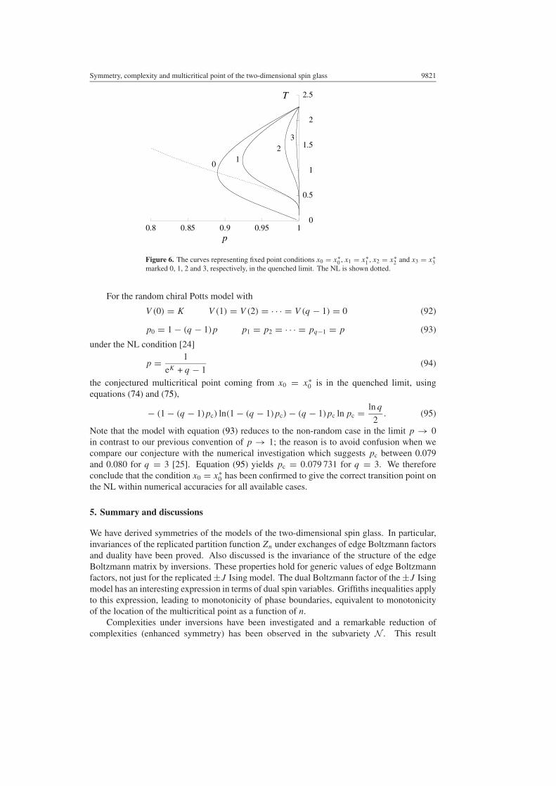
Interestingly, the curve (83) coming from x0 = x∗0 is the only one with an intersection

with the NL in the quenched limit. All the other curves xk = x∗k (k � 1) do not cross the NL

as depicted in figure 6.If we further apply the condition x0 = x∗

0 to a model with continuous distribution ofcoupling as in equation (69), we find in the limit n → 0∫

duP (u) ln(1 + e−2βu) = ln 2

2. (90)

This expression already appeared in [23]. Under the NL condition (71), this equation reads∫du eβuF (u2) ln(1 + e−βu) = ln 2

2(91)

which gives for the Gaussian model J0/J = 1.021 77. Numerical results are consistent withthis value, 1.00(2) (Y Ozeki et al private communication).


0.8 0.85 0.9 0.95 10

0.5

1

1.5

2

2.5

p

T

01

23

Figure 6. The curves representing fixed point conditions x0 = x∗0 , x1 = x∗

1 , x2 = x∗2 and x3 = x∗

3marked 0, 1, 2 and 3, respectively, in the quenched limit. The NL is shown dotted.

For the random chiral Potts model with

V (0) = K V (1) = V (2) = · · · = V (q − 1) = 0 (92)

p0 = 1 − (q − 1)p p1 = p2 = · · · = pq−1 = p (93)

under the NL condition [24]

p = 1

eK + q − 1(94)

the conjectured multicritical point coming from x0 = x∗0 is in the quenched limit, using

equations (74) and (75),

− (1 − (q − 1)pc) ln(1 − (q − 1)pc) − (q − 1)pc ln pc = ln q

2. (95)

Note that the model with equation (93) reduces to the non-random case in the limit p → 0in contrast to our previous convention of p → 1; the reason is to avoid confusion when wecompare our conjecture with the numerical investigation which suggests pc between 0.079and 0.080 for q = 3 [25]. Equation (95) yields pc = 0.079 731 for q = 3. We thereforeconclude that the condition x0 = x∗

0 has been confirmed to give the correct transition point onthe NL within numerical accuracies for all available cases.

5. Summary and discussions

We have derived symmetries of the models of the two-dimensional spin glass. In particular,invariances of the replicated partition function Zn under exchanges of edge Boltzmann factorsand duality have been proved. Also discussed is the invariance of the structure of the edgeBoltzmann matrix by inversions. These properties hold for generic values of edge Boltzmannfactors, not just for the replicated ±J Ising model. The dual Boltzmann factor of the ±J Isingmodel has an interesting expression in terms of dual spin variables. Griffiths inequalities applyto this expression, leading to monotonicity of phase boundaries, equivalent to monotonicityof the location of the multicritical point as a function of n.

Complexities under inversions have been investigated and a remarkable reduction ofcomplexities (enhanced symmetry) has been observed in the subvariety N . This result


suggests that the behaviour of the system is simpler in this subvariety than at generic pointseven if the problem is not (generically) integrable because the exponential growth excludesintegrability.

Conjecture on the exact location of the multicritical point on the NL has been presentedbased on the duality and symmetry arguments. Reasons have been explained why theintersection of the curve x0 = x∗

0 and the NL is the only plausible candidate for the multicriticalpoint among a set of similar conjectures (xk = x∗

k plus the NL). Numerical results are in verygood agreement with this conjecture. Nevertheless, recalling the situation already encounteredfor the analysis of the phase diagram of the isotropic three-state chiral Potts model [27, 28],where the critical manifold is numerically extremely close to the self-dual condition x∗

0 = x0

but is possibly mathematically different (in contrast with the situation encountered in thesymmetric Ashkin–Teller model), one cannot discard the possibility that, restricted to the NL,the transition point could be numerically extremely close to the intersection with x∗

0 = x0

but, actually, mathematically different. These points need to be further investigatedcarefully.

It may be useful to consider the possibility that the condition x0 = x∗0 could be a very

good approximation of the transition manifold away from the intersection with N but in thehigh-temperature part of the phase boundary as in figure 3 at least for random ferromagneticspin systems. For the q-state random standard ferromagnetic Potts model (the random versionof the ferromagnetic scalar Potts model), the condition x0 = x∗

0 in the quenched limit is∫dµ(eK) ln

(eK + (q − 1)

eK

)= 1

2ln q (96)

where the positive interaction K is assumed to be distributed with measure dµ(eK). This isa Potts-generalization of equation (90). Investigation of the consequences of this equation isgoing on.

Another interesting observation is that the formula (84) gives K as a function of n whichdiverges as n approaches −1. It is not obvious at all that we can apply this formula to sucha limit, but if we do so, then the divergence of K implies that the transition point on the NLis T (n)

c → 0 as n → −1. If we use the relation between n and n + 1 in equation (58), wefind that the transition point of the n → 0 (quenched) system vanishes at p = 1

2 . Althoughwe should be very careful in applying our results to such a limit of negative n, this last resultis reasonable and interesting in its own right because it supports the usual consensus that thetwo-dimensional Ising spin glass does not have a finite-temperature phase transition whenthe distribution of bond randomness is symmetric. More efforts should be devoted to theinvestigation of this problem.

Let us also comment here on the equivalence between the n-replicated 3d random latticegauge theory and its dual, the n-replicated Ising spin ferromagnet with edge Boltzmann factordescribed in section 2.6. All the arguments of sections 2.6 and 2.7 apply to such a case.In particular the bound on the critical probability like (54) results: p(0)

c (MCP) � 0.9005.Numerically it is 0.97 [26]10.

We have seen that the replica analysis naturally yields for consideration a class ofremarkable (non-random) lattice spin models, defined by equation (6), which are highlystructured and for which extensive symmetry analysis can be performed exactly. RecallingDomany’s (Nα,Nβ) terminology [29], these models correspond to highly symmetric specific(N2, . . . , N2) models and, more generally, (Nq, . . . , Nq) models. These singled-out classes oflattice spin edge models provide a very powerful tool of analysis for many spin-glass problemsand are also worth studying per se.10 This value is for the T = 0 transition point, not for the multicritical point, but is likely to be close to the latter.


One should note that many of the exact calculations displayed in this paper are stillvalid when the distribution of the coupling constants is not of ±J type or some continuousdistribution like equation (71) but, for instance, a two-delta-peaks (J1, J2) distribution, or,even, a totally general distribution: we only need to get an effective Boltzmann matrix ofthe hierarchical form (6). One should also underline that these models can straightforwardlybe generalized to chiral Potts models (see appendix B), and also to spin models without anyWu–Wang duality (such as the Ising model with a magnetic field, see appendix B; the nonlinearinversion relations I and J taking the place of the linear duality transformation D), providingroom for many new exact results on spin-glass problems.

Acknowledgments

The work of HN was supported by the grant-in-aid for Scientific Research by the Ministry ofEducation.

Appendix A

In this appendix we outline the proof of equation (40) assuming equation (34) and the symmetry(24) under the operation M. According to the duality relation (15) for even n = 2q, theexpression of x∗

m, after applying the operation M, reads

2qx∗m =

q∑k=0

D2km x2k +

q∑k=1

D2k−1m x2k−1

→q∑

k=0

D2km x2k +

q∑k=1

D2k−1m x2q−2k+1

= D0mx0 + D2

mx2 + D4mx4 + · · · + D2q

m x2q+ D1mx2q−1 + D3

mx2q−3 + · · · + D2q−1m x1. (A.1)

We then impose the condition (34) to find

2qx∗m = D0

mx0 +(D1

m + D2m

)x2 +

(D3

m + D4m

)x4 + · · · +

(D2q−1

m + D2qm

)x2q . (A.2)

Thus, in order to show x∗m = x∗

2q−m+1, it suffices to derive

D2k−1m (2q) + D2k

m (2q) = D2k−12q−m+1(2q) + D2k

2q−m+1(2q) (A.3)

where we have written the n(= 2q)-dependence explicitly. This equation can be proved byinduction with respect to q.

The following relation will be useful for the proof:

Dkm+1(n) + Dk−1

m+1(n) = Dkm(n) − Dk−1

m (n) (A.4)

which is derived by replacing m in equation (16) with m + 1 (which amounts to multiplyingboth sides by (1 − t)/(1 + t)).

It is easy to check explicitly using equation (17) that the target relation (A.3) is valid forsmall q with any m and k. Let us then assume that this equation holds for q with any m and kand show that the same is true for q + 1. The left-hand side of equation (A.3) with 2q replacedby 2q + 2 can be reduced to an expression with 2q using the recursion relation (39) twice,

D2k−1m (2q + 2) + D2k

m (2q + 2) = D2km (2q) + D2k−1

m (2q) + 2(D2k−1m (2q) + D2k−2

m (2q))

+ D2k−2m (2q) + D2k−3

m (2q). (A.5)


Application of the other recursion relation (A.4) to each pair of terms on the right-hand sideof the above equation yields

D2k−1m (2q + 2) + D2k

m (2q + 2) = D2km−1(2q) + D2k−1

m−1 (2q) − D2k−2m−1 (2q) − D2k−3

m−1 (2q). (A.6)

This is our expression for the left-hand side of equation (A.3) with q → q + 1. The right-handside of equation (A.3) with 2q replaced by 2q + 2 can also be rewritten by the recursions (39)and (A.4) to reach a similar expression

D2k−12q+2−m+1(2q + 2) + D2k

2q+2−m+1(2q + 2)

= D2k2q−m+2(2q) + D2k−1

2q−m+2(2q) − D2k−22q−m+2(2q) − D2k−3

2q−m+2(2q). (A.7)

This equation is equal to equation (A.6) by the starting assumption of induction, whichcompletes the proof.

Appendix B

The results on the Ising model generalize straightforwardly to q-state models. Let us consider,for instance, the three-state chiral Potts model corresponding to a 3×3 cyclic edge Boltzmannmatrix11. For an arbitrary number n of replicas, the previous hierarchical scheme generalizesstraightforwardly. If one denotes by An the qn × qn effective edge Boltzmann matricescorresponding to [Zn]av they can be obtained by the following recursion:

An → An+1 =An Bn Cn

Cn An Bn

Bn Cn An

(B.1)

where

A1 =x0,0 x0,1 x1,0

x1,0 x0,0 x0,1

x0,1 x1,0 x0,0

(B.2)

and

Bn = An(xm,p → xm,p+1) Cn = An(xm,p → xm+1,p).

Note that the number of homogeneous parameters necessary to describe the pattern (B.1)grows quadratically with the number of replicas like (n + 2)(n + 1)/2 (this number is 3 forn = 1, 6 for n = 2, 10 for n = 3, 15 for n = 4, 21 for n = 5, . . . ). The family of 3n × 3n

models we have to study is thus a little more complicated (as well as the equivalent of thesubvarieties N (34)). This is in contrast with the q = 2 Ising model without magnetic field,analysed in the text, for which the number of homogeneous parameters xk grows linearly withn (this number is n+1). More generally, for a cyclic q×q matrix, the number of homogeneousparameters necessary to describe a pattern generalizing (B.1) will be the number of partitionsof n into q natural integers ki : k1 = k2 + k3 + · · · + kq = n with ki = 0, 1, . . . , n. Theduality transformation on these models (B.1) is inherited from the duality transformation onthe three-state chiral Potts model associated with cyclic 3 × 3 matrices.

Let us consider a simple example of a spin edge model with no duality transformation,namely the Ising model with a magnetic field. The effective Boltzmann matrices can beobtained similarly by a hierarchical scheme generalizing (6):

An → An+1 =[An Bn

Bn Cn

](B.3)

11 That is the chiral Potts model studied by Baxter et al [30].


where

A1 =[x0,0 x1,0

x1,0 x0,1

](B.4)

and

Bn = An(xm,p → xm+1,p) Cn = An(xm,p → xm,p+1).

Again the number of homogeneous parameters necessary to describe the pattern (B.3) growsquadratically with the number of replicas like (n + 2)(n + 1)/2. In this last case, we do nothave a duality transformation D anymore: the inversion relations I and J take the place ofthe linear duality transformation D. However, the inverses of matrices given by (B.3) are notmatrices of the same form (B.3). One thus needs to consider slightly more general matricesthan (B.3) in order to be able to use the nonlinear symmetry I . Details will be given elsewhere.

References

[1] Mezard M, Parisi G and Virasoro M A 1987 Spin Glass Theory and Beyond (Singapore: World Scientific)[2] Young A P (ed) 1997 Spin Glasses and Random Fields (Singapore: World Scientific)[3] Nishimori H 1981 Prog. Theor. Phys. 66 1169[4] Nishimori H 2001 Statistical Physics of Spin Glasses and Information Processing: An Introduction (Oxford:

Oxford University Press)[5] Angles d’Auriac J-Ch, Maillard J-M and Viallet C M 2002 J. Phys. A: Math. Gen. 35 9251[6] Wu F Y and Wang Y K 1976 J. Math. Phys. 17 439[7] Georges A, Hansel D, Le Doussal P and Maillard J-M 1987 J. Physique 48 1[8] Meyer H, Angles d’Auriac J-Ch, Maillard J-M and Rollet G 1994 Physica A 208 223[9] Boukraa S and Maillard J-M 2001 J. Stat. Phys. 102 641

[10] Nishimori H 2002 J. Phys. A: Math. Gen. 35 9541[11] Griffiths R B 1972 Phase Transitions and Critical Phenomena vol 1 ed C Domb and M S Green (London:

Academic)[12] Nishimori H 1986 J. Phys. Soc. Japan 55 3305[13] Abarenkova N, Angles d’Auriac J-Ch, Boukraa S and Maillard J-M 1999 Physica D 130 27[14] Abarenkova N, Angles d’Auriac J-Ch, Boukraa S, Hassani S and Maillard J-M 1999 Physica A 264 264[15] GNU Multiprecision; see http://www.swox.com/gmp/

[16] Nishimori H and Nemoto K 2002 J. Phys. Soc. Japan 71 1198[17] Ozeki Y, Kasono K, Ito N and Miyashita S 2003 Physica A 321 271[18] Ito N and Ozeki Y 2003 Physica A 321 262[19] Aarao Reis F D A, de Queiroz S L A and dos Santos R R 1999 Phys. Rev. B 60 6740[20] Singh R R P and Adler J 1996 Phys. Rev. B 54 364[21] Honecker A, Picco M and Pujol P 2001 Phys. Rev. Lett. 87 047201[22] Merz F and Chalker J T 2002 Phys. Rev. B 65 054425[23] Nishimori H 1979 J. Phys. C: Solid State Phys. 12 L905[24] Nishimori H and Stephen M J 1983 Phys. Rev. B 27 5644[25] Jacobsen J L and Picco M 2002 Phys. Rev. E 65 026113[26] Wang C, Harrington J and Preskill J 2003 Ann. Phys., NY 303 31[27] Angles d’Auriac J-Ch, Maillard J-M and Wu F Y 1991 Physica A 177 114[28] Angles d’Auriac J-Ch, Maillard J-M and Wu F Y 1991 Physica A 179 496[29] Domany E and Riedel E K 1978 Phys. Rev. Lett. 40 561[30] Baxter R J, Perk J H H and Au-Yang H 1988 Phys. Lett. A 128 138

fulltext.calis.edu.cnfulltext.calis.edu.cn/iop/0305-4470/36/38/301/a33801.pdf · INSTITUTE OF...

Documents

Transcript of fulltext.calis.edu.cnfulltext.calis.edu.cn/iop/0305-4470/36/38/301/a33801.pdf · INSTITUTE OF...