INFLUENCE OF MAGNETIC FIELD ON DIELECTRIC SUSCEPTIBILITY OF

AMORPHOUS SOLIDS AT ULTRA LOW TEMPERATURE

A DISSERTATION

SUBMITTED TO THE DEPARTMENT OF PHYSICS

AND THE COMMITTEE ON GRADUATE STUDIES

OF STANFORD UNIVERSITY

IN PARTIAL FULFILLMENT OF THE REQUIREMENTS

FOR THE DEGREE OF

DOCTOR OF PHILOSOPHY

Lidiya V. Polukhina

December 2009

http://creativecommons.org/licenses/by-nc/3.0/us/

This dissertation is online at: http://purl.stanford.edu/tj926rq2834

© 2010 by Lidiya Vladimirovna Polukhina. All Rights Reserved.

Re-distributed by Stanford University under license with the author.

This work is licensed under a Creative Commons Attribution-Noncommercial 3.0 United States License.

ii

I certify that I have read this dissertation and that, in my opinion, it is fully adequatein scope and quality as a dissertation for the degree of Doctor of Philosophy.

Douglas Osheroff, Primary Adviser

I certify that I have read this dissertation and that, in my opinion, it is fully adequatein scope and quality as a dissertation for the degree of Doctor of Philosophy.

Blas Cabrera

I certify that I have read this dissertation and that, in my opinion, it is fully adequatein scope and quality as a dissertation for the degree of Doctor of Philosophy.

John Lipa

Approved for the Stanford University Committee on Graduate Studies.

Patricia J. Gumport, Vice Provost Graduate Education

This signature page was generated electronically upon submission of this dissertation in electronic format. An original signed hard copy of the signature page is on file inUniversity Archives.

iii

iv

ABSTRACT

The dielectric response of some amorphous solids below 100 mK is known to be

sensitive to an applied magnetic field. This work presents new experimental data on the

behavior of BK7, Aluminum-Barium-Silicate, Suprasil, Corning® microscope cover

glass and Mylar® film (amorphous Polyethylene Terephthalate) samples in the

temperature range from 2 mK to 100 mK in presence of a slowly varying magnetic field.

We studied the dielectric constant by means of continuous wave AC capacitance

measurements at 1 kHz. We observed hysteresis in the dielectric response to a magnetic

field varying in a saw-like pattern with field strengths up to 2 milliTesla. The pattern of

the response differs depending on the glass composition. The results presented in this

work are consistent with previously made observations that nuclear spins greater than ½

play a crucial role in the observed magnetic field dependence.

v

ACKNOWLEDGMENTS

There are many people who I would like to thank for having contributed to the

completion of this thesis. First of all, my sincerest gratitude goes to my thesis advisor,

Doug Osheroff, who provided me the best opportunity to learn the knowledge and skills

in low temperature physics. His patience with my learning process was amazing. His

enthusiasm and positive attitude has always been admirable and the most encouraging at

the difficult times.

I am grateful to John Lipa, Sandy Fetter and Blas Cabrera for taking the time out

of their busy schedule to read through my thesis and providing me with helpful

comments. I would also like to thank James Harris for serving as a chair of my University

Oral Examination Committee.

I was fortunate to be in communication with Alex Burin, Yurii Sereda and Il’ya

Polishchuk who have been studying the subject of this work theoretically. Discussions

with them were invaluable for my understanding of glass theory.

I wish to thank the group members with whom I worked most closely and who I

learned a lot from. Barry Barker welcomed me to the group and spent many hours

transferring to me many skills and his enjoyment of experimental physics. Danna

Rosenberg had taught me an amazing number of details about the glasses project in the

vi

short time of our overlap on it. Seunghwa Ryu’s contribution to data taking was

absolutely invaluable. His ability to remain concentrated on the task at hand for countless

hours and to approach the problem systematically helped this project to succeed. Viktor

Tsepelin had taught me many good practices in low temperature mechanical design.

Qiang Qu, Arito Nishimori, James Baumgardner and Benjamin Shank were great

teammates and friends when it came to dealing with the liquefier, pumps and

compressors or simply dealing with stressful times.

Thanks to the department staff including Maria Frank, Rosenna Yau, Jennifer

Tice, Cindy Mendel, Stewart Kramer and especially Marcia Keating for making the

administrative tasks easier. This work would not have been possible without Karlheinz

Merkle, Matthew Chuck and Mehmet Solyali, machinists in the Varian shop. I always

admired their attitude as professionals. Not only they machined countless parts for the

experiment, saved our equipment with ingenious repairs on numerous occasions, but also

taught me a lifetime skill of machining and soldering.

I enjoyed the friendship with my classmates Sergey Prokushkin, Alex

Kretchetov, Deborah Berebichez and many others. It is the interaction with fellow

graduate students that helped me the most in learning to think like a physicist. Nikolai

Lehtinen have supported and encouraged me at the earlier years of grad school. Leonid

Litvak and Robert Rudnitsky helped me to stay on top of things when it seemed like

things are falling apart. Nella Shapiro kept me company at the stage of writing,

vii

encouraging me and helping me to work more effectively. Eugene Fooksman helped me

with my final software struggle.

Stanford Ballroom Dance Team played an important role in my graduate life.

Through the Team, I’ve made many friends as well as learned valuable leadership skills.

The Team had provided a nice stress relief and a balancing force. My dance partner of

many years Alex Vasserman had helped me on numerous occasions like putting up the

radiation shields and inner vacuum can as well as helped me to retain my sanity with

regular dance practices.

My family has always been the most important source of inspiration and support

for me despite of being far away. I couldn’t have accomplished it without feeling their

strength. Lyudmila Polukhina, my wise and loving mother, a physicist and a role model,

always cheerful and optimistic, had always been encouraging and supporting. My brother

Nikolai had always cheered me on with jokes and stories. My father wanted me to

complete this project and I couldn’t fail him on that even though he didn’t live long

enough to see it finished.

This work was supported by Department Of Energy under grant number DE-

FG03-90ER435.

viii

TABLE OF CONTENTS

Abstract .............................................................................................................................. iv

Acknowledgments................................................................................................................v

List of tables .........................................................................................................................x

List of figures ..................................................................................................................... xi

CHAPTER 1. Introduction ............................................................................................1

CHAPTER 2. Theory and Motivation: Introducing Interactions to the Standard

Tunneling Model ............................................................................................................4

2.01 The TLS Hamiltonian and Density of States. Non-interacting model ...............4

2.02 The Effects of Nuclear Quadrupole Interactions on Resonant

Susceptibility..........................................................................................................18

CHAPTER 3. Experimental Setup ..............................................................................32

3.01 Glass samples ...................................................................................................32

3.02 Fridge and cooling techniques .........................................................................35

3.03 Experimental Cell ............................................................................................39

3.04 Magnet .............................................................................................................40

3.05 Bridge measurement ........................................................................................41

CHAPTER 4. Measurement and Observations ...........................................................45

4.01 Aluminum-Barium-Silicate. .............................................................................45

4.02 Suprasil, Mylar .................................................................................................51

4.03 Hysteresis on AlBaSi .......................................................................................54

4.04 BK7 ..................................................................................................................66

4.05 Corning ............................................................................................................72

CHAPTER 5. Discussion ............................................................................................74

CHAPTER 6. Conclusions and future work. ..............................................................77

APPENDIX A: Cryogenic JFET .....................................................................................79

ix

APPENDIX B: Capacitance versus temperature, zero magnetic field ............................81

APPENDIX C: Relaxation measurements .......................................................................82

BIBLIOGRAPHY ..............................................................................................................86

x

LIST OF TABLES

Number Page

Table 2.1 Saturation temperature satT for various glasses below which the dielectric

constant ε becomes temperature independent. .................................................24

Table 3.1 Samples used in our magnetic field effects experiment. ...................................33

Table 3.2 Change in dielectric constant per decade in temperature. .................................34

Table 5.1 Chemical composition of glass samples. ...........................................................75

xi

LIST OF FIGURES

Number Page

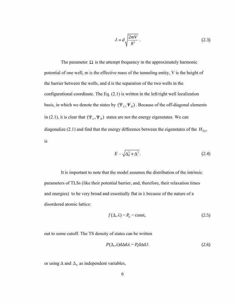
Figure 2.1 Two levels of energy; no assumptions are made about the shape of the

potential..............................................................................................................8

Figure 2.2 Temperature Variation of the Dielectric Constant of AlBaSi glass

measured at 1 kHz [19]. ...................................................................................13

Figure 2.3 Capacitance vs Temperature, SiOx [34]. ..........................................................14

Figure 2.4 Dielectric Response of Mylar at 5 kHz [29]. ....................................................15

Figure 2.5 The Two Level System. ....................................................................................20

Figure 2.6 Two level configuration with split energy levels. [41] .....................................23

Figure 2.7 Influence of the magnetic field on the dielectric constant of the BaO-

Al2O3-SiO2 glass ............................................................................................25

Figure 2.8 Energy levels in TLS (a) in absence and (b) in presence of an applied

magnetic field...................................................................................................27

Figure 2.9 Magnetic field B is perpendicular to the EFG axes in left and right

potential wells ..................................................................................................29

Figure 2.10 Temperature dependence of the contribution to the permittivity of

tunneling systems due to the quadrupole interaction [41]. ..............................31

Figure 3.1 The Cryogenic JFET, Experimental Cell and MCT mounted on the

cryostat .............................................................................................................36

Figure 3.2 Experimental Cell. (Built by D. Rosenberg) [33] .............................................37

Figure 3.3 Idealized representation of a variable ratio capacitance bridge, with sample

capacitance Csample and reference capacitance Cref ...........................................42

Figure 4.1. Small Magnetic Field, AlBaSi, E = 4.5 kV/m, T = 5.6 mK. ...........................47

Figure 4.2 Typical Magnetic Field Sweep, AlBaSi, E = 4.5 kV/m, T = 5.6 mK. ..............49

Figure 4.3 Magnetic Field Sweep, AlBaSi, E = 4.5 kV/m, T = 1.47 mK. .........................50

Figure 4.4 Suprasil, E = 3.9 kV/m, T = 5.8 mK ................................................................52

xii

Figure 4.5 Mylar, E = 2.25 kV/m, T = 12.7 mK ................................................................53

Figure 4.6 Hysteresis on AlBaSi, E = 4.5 kV/m, T = 5.6 mK. ..........................................55

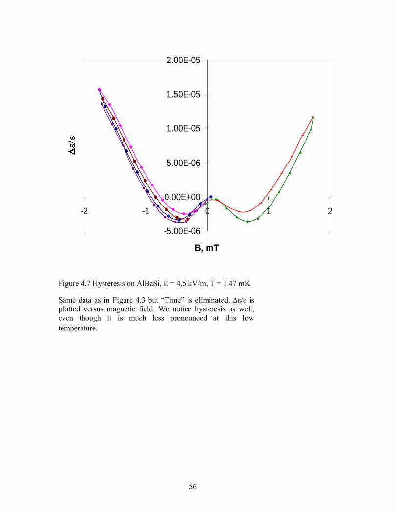
Figure 4.7 Hysteresis on AlBaSi, E = 4.5 kV/m, T = 1.47 mK. ........................................56

Figure 4.8 AlBaSi Hysteresis Loops, Very Low Temperatures, E = 4.5 kV/m ................57

Figure 4.9 AlBaSi Hysteresis Loops, Intermediate Temperatures, E = 4.5 kV/m .............58

Figure 4.10 Role of the Excitation Voltage / Drive Fields in the Dielectric Response

of AlBaSi Sample. ...........................................................................................59

Figure 4.11 Role of the Excitation Voltage / Drive Fields in the Dielectric Response

of AlBaSi Sample, low excitation voltages. ....................................................60

Figure 4.12 Typical picture of ∆ε/ε vs B, with hysteresis, AlBaSi, E = 2.25 kV/m, T =

4.15 mK............................................................................................................61

Figure 4.13 AlBaSi hysteresis curves, various temperatures, E = 2.25 kV/m. ..................62

Figure 4.14 AlBaSi Hysteresis Loops, Higher Temperatures, E = 2.25 kV/m ..................63

Figure 4.15 Area of hysteresis loops, AlBaSi. ...................................................................65

Figure 4.16 Typical sweep of magnetic field on BK7, E = 2.14 kV/m, T = 4.6 mK. .......67

Figure 4.17 Typical sweep of magnetic field on BK7: hysteresis, E = 2.14 kV/m, T =

4.6 mK..............................................................................................................68

Figure 4.18 BK7 Hysteresis Loops, Various Temperatures, E = 2.14 kV/m. ...................69

Figure 4.19 BK7 hysteresis loops, various temperatures, E = 4.28 kV/m. ........................70

Figure 4.20 Maximum change in dielectric constant due to applied field or 1.8 mT at

different temperatures. .....................................................................................71

Figure 4.21 Corning hysteresis loops, E = 2.14 kV/m. ......................................................73

Figure 6.1 Electronic measurement setup ..........................................................................80

Figure 6.2 Capacitance vs temperature, AlBaSi. ...............................................................81

Figure 6.3 AlBaSi, E = 4.5 kV/m, T = 5.6 mK. Sweep in steps. .......................................83

Figure 6.4 AlBaSi, E = 4.5 kV/m, T = 5.6 mK. Sweep in steps, ∆ε/ε vs B .......................84

Figure 6.5 AlBaSi, E = 4.5 kV/m, T = 8.7 mK. Relaxation of the dielectric constant at

various values of applied magnetic field. ........................................................85

1

CHAPTER 1.

INTRODUCTION

The physical properties of amorphous solids at low temperatures have been

subjects of interest for many decades. Ever since Pohl and Zeller’s discovery of

deviations of the temperature dependences of the specific heat and thermal conductivity

of glasses [27] from T and T2 respectively there have been more and more findings of

universal behavior of glasses in dielectric and acoustic properties of amorphous solids at

low temperatures. A two level system model of tunneling defects with a double well

potential originally proposed by Anderson, Halperin and Varma [1], and independently

by Phillips [11] is now the commonly accepted method of treatment for amorphous

solids at low temperatures. While the model makes no effort to explain the actual

microscopic behavior of glass, nor does it address the origin of the universality, it does

an excellent job of describing many of the observed low temperature properties.

However, due to recent findings, for example magnetic field effects [13-19], dephasing

of coherent echoes [18, 19], and anomalous frequency dependence of the internal

friction [30] the model is having new corrections added [20, 28, 31].

In 1998, Strehlow et al [8] discovered an anomalously high sensitivity of

dielectric properties of several insulating glasses to applied magnetic field at ultra low

temperatures. Since the possibility of magnetic impurities was quickly ruled out, it was

2

evident that the effect arises due to the glass structure itself. It’s been suggested that a

phase transition occurs at 5.84 mK for BaO-Al2O3-SiO2 glass, but further investigations

were needed to confirm it. The effects (but no phase transition) were also observed in

BK7 glass [17].

Although the theoretical explanation for observed phenomena was proposed

[20, 28] the nature of the phenomena was not completely clear. It would have been

interesting to know, for example, if all glasses respond to magnetic fields in a similar

fashion, and if there is a correlation with previously found anomalies like independence

of the dielectric susceptibility of temperature at the very low temperature (T ≤ 5 mK)

and with the slope in the temperature dependence of the dielectric constant.

This experimental work is a survey of five different glasses subjected to

varying magnetic field. Although we were unable to confirm the mentioned phase

transition, we found a rich variety magnetic dependent responses occurring in glasses in

the temperature region of 1mK < T < 10 mK.

The structure of this thesis is straight-forward. Chapter 2 contains brief

theoretical introduction to the two-level system model describing amorphous solids at

low temperatures. First, non-interacting model is introduced. Since it appears to be

insufficient to describe the phenomena of interest, the effect of interactions is

considered. Since this work is concentrating on dielectric properties, we don’t discuss

other phenomena in amorphous solids at low temperature. Chapter 3 describes the

experimental apparatus and discusses its advantages and limitation. Chapter 4 reports on

3

measurements. We observed the magnetic field effect in AlBaSi, BK7 and Corning. We

didn’t see it in Suprasil and Mylar. Each of the three samples where the effect was seen

is treated in a separate section. There is a section on Suprasil and Mylar, but there isn’t

much data to present since they don’t demonstrate said effect. We conclude this work

with discussion in Chapter 5.

4

CHAPTER 2.

THEORY AND MOTIVATION: INTRODUCING INTERACTIONS TO THE

STANDARD TUNNELING MODEL

This chapter will review a commonly accepted model for studying amorphous

solids at low temperatures. The non-interacting model fits well with the early

experiments that show the difference between amorphous solids and crystalline solids in

specific heat and thermal conductivity. However, later experiments show that

interactions play an important role and cannot be neglected altogether for studying the

behavior of dielectric properties at low temperatures.

2.01 THE TLS HAMILTONIAN AND DENSITY OF STATES. NON-

INTERACTING STANDARD TUNNELING MODEL

One of more unexpected results in solid state physics was provided by the

research of Zeller and Pohl on the heat capacity and thermal conductivity in a number

of glasses below 1 K [27]. Before their research it had been argued that because low

temperature properties are dominated by phonons (quantized lattice vibrations) of low

frequency, and because in crystals these phonons can be described as long-wavelength

sound waves propagating through an elastic continuum, there should be little difference

between glasses and crystals in this regime where phonons are insensitive to

microscopic structure. However, their measurements and their extensive literature

5

search of the previous studies have revealed that instead of Debye specific heat these

systems are dominated by a semi-linear term at low temperature, 1.2 3C T T .

Anderson, Halperin and Varma, and independently Phillips [1, 3] developed a model

attributing the additional terms in the heat capacity and thermal conductivity to the

existence of defects due to disorder which are not present in crystals. In their model the

defects are represented by non-interacting two-level systems with a distribution of

energy splittings and tunneling barriers. This model assumed the name “Standard

Tunneling Model” (STM) and became common to use for studying low temperature

properties of amorphous solids. (See, for example, [1-4], [8]). The description of the

basic TLS model below will closely follow [4].

The tunneling systems (we imply quantum tunneling) in amorphous

solids are atoms or small groups of atoms that have a possibility to “move” between two

similar low lying energy states separated by a barrier. Usually, if one wants to

emphasize their two level nature, the term “two-level system”, or TLS, is used to denote

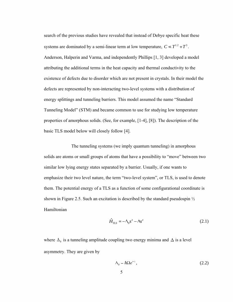
them. The potential energy of a TLS as a function of some configurational coordinate is

shown in Figure 2.5. Such an excitation is described by the standard pseudospin ½

Hamiltonian

0

ˆ x z

TLSH s s (2.1)

where 0 is a tunneling amplitude coupling two energy minima and is a level

asymmetry. They are given by

0 ,ћ e (2.2)

6

2

2mVd

ћ. (2.3)

The parameter is the attempt frequency in the approximately harmonic

potential of one well, m is the effective mass of the tunneling entity, V is the height of

the barrier between the wells, and d is the separation of the two wells in the

configurational coordinate. The Eq. (2.1) is written in the left/right well localization

basis, in which we denote the states by ( , )L R . Because of the off-diagonal elements

in (2.1), it is clear that ( , )L R states are not the energy eigenstates. We can

diagonalize (2.1) and find that the energy difference between the eigenstates of the TLSH

is

2 2

0 .E (2.4)

It is important to note that the model assumes the distribution of the intrinsic

parameters of TLSs (like their potential barrier, and, therefore, their relaxation times

and energies) to be very broad and essentially flat in λ because of the nature of a

disordered atomic lattice:

0( , ) const, f P (2.5)

out to some cutoff. The TS density of states can be written

0( , )d d d dP P (2.6)

or using Δ and 0 as independent variables,

7

00 0 0

0

( , )d d d dP

P (2.7)

Said uniform distribution of parameters Δ and 0 is one of the main assumptions of the

standard model. High energy cutoffs need to be introduced for Δ and 0 to avoid an

unphysical divergence of the density of states, and this cutoff W is usually assumed to

be on the order of 50B

Wk

K where the TLS are no longer the dominant excitation

and therefore seize to be of importance. Similarly, a lower limit for 0 is needed, since

0

1P . The value of 0,min is not known but is usually assumed to be very small, on

the order of several microkelvin.

The distribution (2.7) leads to universal temperature and time dependencies for

various physical characteristics of amorphous solids. The properties 2T along with

c T that follow directly from this model [1-4] are considered to be among the main

characteristics of glassy behavior at low temperatures. Although these properties are

well known and thoroughly described in the literature [1-4], they are briefly discussed

below for the completeness of this text.

2.01.1 THERMODYNAMIC PROPERTIES OF TSL: HEAT CAPACITY

Let’s consider a TLS with the level splitting E. The partition function of such single

TLS can be written as

2 2 2cosh2

E E

kT kTE

Z e ekT

(2.8)

Mean energy for one TLS is therefore

2 ln 1tanh

2 2

Z EU kT E

T kT (2.9)

and the specific heat for a single TLS is

2

2

1 sech2 2

V

V

U E EC k

T kT kT (2.10)

8

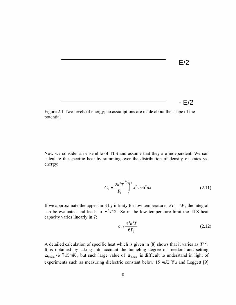
Figure 2.1 Two levels of energy; no assumptions are made about the shape of the

potential

Now we consider an ensemble of TLS and assume that they are independent. We can

calculate the specific heat by summing over the distribution of density of states vs.

energy:

2 2

2 2

0 0

2sech

WkT

V

k TC x dx

P (2.11)

If we approximate the upper limit by infinity for low temperatures kT W , the integral

can be evaluated and leads to 2 /12 . So in the low temperature limit the TLS heat

capacity varies linearly in T:

2 2

06

k Tc

P (2.12)

A detailed calculation of specific heat which is given in [8] shows that it varies as 1.2T .

It is obtained by taking into account the tunneling degree of freedom and setting

0,min / 15k mK , but such large value of 0,min is difficult to understand in light of

experiments such as measuring dielectric constant below 15 mK. Yu and Leggett [9]

E/2 - E/2

9

showed that it is also possible to obtain a superlinear heat capacity by introducing

pseudogap in the density of states at low energies.

2.01.2 THERMODYNAMIC PROPERTIES OF TLS: THERMAL CONDUCTIVITY

In general, kinetic theory gives the thermal conductivity of any material as

1

3cvl , (2.13)

where c is the specific heat per unit volume of the excitation that carry the heat, v is

their characteristic velocity, and l is their mean free path. In insulators, thermal energy

is transferred mainly by phonons. Phonons propagate at the speed of sound. In

crystalline insulators, their mean free path is determined by scattering off the lattice

imperfections and by sample boundaries, and is temperature independent. In amorphous

solids, we assume that phonons are still the dominant carriers of thermal energy. They

are scattered by TLS. In order to find the thermal conductivity we need to calculate the

phonon mean free path in presence of TLS. The sound velocity can be measured.

The phonon mean free path is set by phonon relaxation time in the system and is

given by l v , where is the mean time a phonon of polarization η travels before

scattering off a TLS. The phonons interact with TLS by deforming their potentials.

Such an elastic wave adds a perturbation interH to the Hamiltonian H (2.1) which in the

( , )L R basis looks as

01

,02

interH (2.14)

if we neglect a possible variation of the off-diagonal matrix element 0 [4]. The change

of the asymmetry is related to the local elastic strain tensor iku

via the coupling constant γ,

2 iku (2.15)

Here we suppressed the tensorial nature of u and wrote its average magnitude. For a

more detailed approach and the general definition of coupling constants see [4], section

4.2.2. Switching to the energy eigenstate basis, we can re-write the complete

Hamiltonian as

10

0 21 1

0 22 2

E D MH u

E M D (2.16)

where

2

DE

(2.17)

0ME

(2.18)

Considering single-phonon transition processes, we can compute the matrix elements

connecting an initial state ;0 (TLS in upper state, no phonon) to the final state

; ,k (TLS in lower state, phonon of wave vector k and polarization η is created).

The matrix element is found to be [10]

0; , ;02

inter

kH

v Ek (2.19)

where ρ is the mass density of the sample and v is the respective sound velocity. With

this matrix element and using Fermi’s Golden rule we obtain the following for the one-

phonon relaxation rate:

2 2 2

1 0

5 5 4

2coth

2 2

l tph

l t B

E E

v v ћ k T (2.20)

The first term is a material-dependent parameter where the indices t and l refer to the

longitudinal and transverse phonon modes, respectively. We denote

2 2

0 4 5 5

1 2

2

l t

l tћ v v (2.21)

The most active TLS are thermal: 0 BE k T . Therefore, one-phonon relaxation rate

for thermal TLS can be approximated as

1 3

0th T (2.22)

The parameter 1

ph defines the rate at which a TLS will emit a phonon in its transition

from high into low state. The rate of resonant absorption of a phonon of polarization η

is given by [11]

11

2

1 2 2

0 0,min2( ) tanh

2 B

ћP ћ

ћ v k T (2.23)

Mean free path is determined by scattering off the TLS, therefore it is related to the rate

at which phonons are absorbed and re-emitted.

( , ) ( , )l T v T (2.24)

With this in mind, we can come back to the subject of thermal conductivity. It can be

written as

0

1( ) ( )

3T d C v l (2.25)

Utilizing the expression for Debye heat capacity given by eq. (5.30) [12]

2 4

22 3 2

3( )

21

B

B

ћ

k T

ћB

k T

Vћ eC

v k Te

(2.26)

and the obtained (2.23), we can re-write the expression for thermal conductivity (2.25)

as

4 3 4

2 3 2

0

( ) ( , )2 ( 1)

Dx x

B

x

k T x eT x T dx

ћ v e (2.27)

where B

ћx

k T, D

D

B

ћx

k T.

As in the specific heat, this calculation is simple enough if one approximates the TLS

density of states vs. energy as flat. Combining (2.27) with (2.23) we notice that the

integral on the right side is just a number, and we see that 2T which is in good

agreement with experimental observations. As it was stated earlier, the properties

2T along with c ~ T are considered to be the main distinctions of glassy behavior at

low temperatures.

12

2.01.3 DIELECTRIC PROPERTIES OF GLASSES, NON-INTERACTING MODEL =

DIELECTRIC AND ACOUSTIC RESPONSE – TEMPERATURE DEPENDENCE.

Dielectric and acoustic (a sound velocity) susceptibilities in glasses show a

logarithmic temperature dependence also associated with the distribution (2.7). The low

temperature acoustic and dielectric responses of amorphous systems are described by

the interaction of the TLS with phonons and external fields. It may be worth mentioning

as a side note that both acoustic and dielectric responses are based on the similar

mechanisms. In the acoustic case all TLSs absorb phonons. In the dielectric case a

subset of these TLSs with permanent electric dipoles interact with an external electric

field in the same fashion. The only difference is the number of the TLSs that are active

[34]. Acoustic properties won’t be discussed in this work, but it is good to be aware of

the similarity of the approach.

Experimental observations showed a typical picture of the dependence of

dielectric constant on temperature. (See, for example, [18, 29, 34].) In most cases, it is a

curve with a well-defined minimum near 50 mK and nearly flat region referred to as

“saturation” at 5 mK and lower. Figure 2.2 – 2.4 show typical results for AlBaSi [19],

SiOx [34], and Mylar [29]. We also measured this dependence for reference purposes,

but since it’s not the main objective of this work, the temperature range was not fully

13

Figure 2.2 Temperature Variation of the Dielectric Constant of AlBaSi glass measured

at 1 kHz [19].

The solid line represents experimental data, the dashed line

represents a calculation with the tunneling model [19].

14

Figure 2.3 Capacitance vs Temperature, SiOx [34].

This graph shows the capacitance at 2.2 kHz vs temperature for

3 µm SiOx sample mounted on sapphire on the top-load slug.

The data show linear behavior in the field for small drive

values. At high levels we see an enhanced low temperature

response that shifts the minimum toward higher temperatures.

There is also a low temperature saturation [34] but we have to

keep in mind that it’s a vacuum mount, not an immersion cell;

the heat sinking is not as good.

15

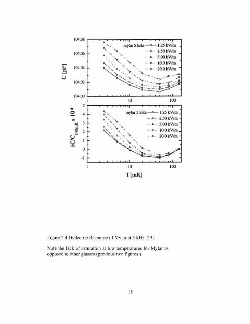
Figure 2.4 Dielectric Response of Mylar at 5 kHz [29].

Note the lack of saturation at low temperatures for Mylar as

opposed to other glasses (previous two figures.)

16

covered in this work as it presented additional challenges. Some experimental results

are shown in Appendix B.

For qualitative understanding, it is useful to think of it in the following terms.

The response of a driven TLS can be divided into two temperature regimes: the

relaxational tunneling regime, where the system is dominated by phonon-assisted

tunneling (higher temperatures), and the resonant tunneling regime (lower

temperatures). In the resonant regime the perturbation due to phonons is sufficiently

small so that resonant (coherent) quantum mechanical tunneling is possible, TLSs are

coherently driven by external fields. The crossover from the relaxational into the

resonant tunneling regime is indicated by a minimum in response.

There is more than one commonly accepted approach in describing this

behavior. Carruzzo, Grannan and Yu [46] and Stockburger [6] use the fact that the

system is analogous to a spin-½ system and apply Bloch equations, with the energy

splitting E taking place of the magnetic field zB and the measuring field taking the

place of the AC magnetic field acB . Jackle [10] and Anthony and Anderson [2]

calculate the energy absorption of the system and use Kramers-Kronig relation to

extract the nondissipative response. Both approaches involve a great deal of algebra and

the interested reader can find the calculations in the original papers as well as several

reviews and theses [47, 48, 2, 49, 32, 29]. We adopt the approach used by Burin’s

group since it seems straight-forward to connect with the phenomena under study. Not

17

only it describes the minimum in capacitance, but also extends to describe low

temperature behavior as well as magnetic field dependence.

A growing number of qualitative deviations from the standard tunneling model

had been observed at very low temperatures. In particular, it is demonstrated in a

number of works [16, 34], [4, p.234] that, for 5T mK the expected logarithmic

temperature dependence of the dielectric constant breaks down and the dielectric

constant becomes approximately temperature independent. This result conflicts with the

logarithmically uniform distribution (2.7) of TLSs over their tunneling amplitudes. To

resolve this problem, one can assume that the distribution of the TLSs have a low

energy cutoff at 0,min 5mK. This assumption, however, contradicts the observation

of very long relaxation times in all glasses. These times (a week or longer) require much

smaller tunneling amplitudes [5] than 5 mK (remember that the TLS relaxation time is

inversely proportional to its squared tunneling amplitude).

A. Burin et al [35] suggest the solution to this discrepancy by using the model

of Würger, Fleischmann and Enss [36] who proposed that the nuclear quadrupole

interactions affect the properties of TLSs at low temperatures by the mismatch of the

nuclear quadrupole states in different potential wells (Figure 2.5) The significance of

nuclear quadrupole interaction for the temperature dependence of the dielectric constant

at T≤ 5 mK will help us understand magnetic field dependence of dielectric properties

of non-magnetic glasses.

18

2.02 THE EFFECTS OF NUCLEAR QUADRUPOLE INTERACTIONS ON

RESONANT SUSCEPTIBILITY

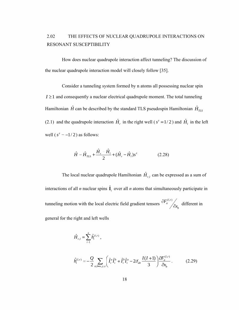
How does nuclear quadrupole interaction affect tunneling? The discussion of

the nuclear quadrupole interaction model will closely follow [35].

Consider a tunneling system formed by n atoms all possessing nuclear spin

1I and consequently a nuclear electrical quadrupole moment. The total tunneling

Hamiltonian H can be described by the standard TLS pseudospin Hamiltonian ˆTLSH

(2.1) and the quadrupole interaction ˆrH in the right well ( 1/ 2zs ) and ˆ

lH in the left

well ( 1/ 2zs ) as follows:

ˆ ˆ

ˆ ˆ ˆ ˆ( )2

zr lTLS r l

H HH H H H s (2.28)

The local nuclear quadrupole Hamiltonian ,

ˆr lH can be expressed as a sum of

interactions of all n nuclear spins ˆiI over all n atoms that simultaneously participate in

tunneling motion with the local electric field gradient tensors ( , )l r

a

b

Fx

different in

general for the right and left wells

( , )

,

1

ˆˆn

l r

r l i

i

H h ,

( , )

( , )

, , ,

( 1)ˆ ˆ ˆ ˆ ˆ 22 3

l rl r a b b a a

i i i i i ab

a b x y z b

Q I I Fh I I I I

x. (2.29)

19

Here ˆa

iI is a nuclear spin projection onto α axis and Q is the electrical

quadrupole moment.1

For the qualitative argument it is sufficient to consider a simplified model for

the nuclear quadrupole interaction (2.29) possessing axial symmetry (See Figure 2.5)

, 2

, ,

( 1)ˆ ( )3

l ru

l r l r

I IH b I (2.30)

where | |Fb Qx

(2.31)

and Lu and Ru are the nuclear quadrupole quantization axes. They define the direction

of the electric field gradient in the left and right wells, respectively.

1 Quadrupole moment of a system is defined as symmetric tensor

2

, (3 r )i k i k ikQ e x x with the sum of diagonal elements equal to zero. Finding the

values of Q requires averaging of this operator over the wave function. In a state with

defined 2I ( 1)I I and z JI M zzQ is also defined and equal to

23 1( 1)

(2 1) 3zz I

QQ M I I

I I. When IM I (projection of momentum is aligned

with z axis) zzQ Q ; this quantity is usually referred to simply as “quadrupole

moment”. [37]

20

Figure 2.5 The Two Level System.

The two level system with well separation d, asymmetry

energy ∆, tunneling amplitude ∆0. The different nuclear

quadrupole quantization axes Lu and Ru are defined by the

local electric field gradient in the left and right wells.

d

∆0

21

Let us now consider a single TLS polarization due to an external electric field

F. Assume that tunneling atoms possess a non-zero charge. Then the tunneling between

the right and the left wells changes the dipole moment of TLS. The TLS dipole moment

operator can be expressed in terms of pseudospin as

ˆ zsμ μ . (2.32)

where µ is a dipole moment of a tunneling system. The interaction of the external field

F with a TLS can be written as

ˆ zV sFμ (2.33)

The effect of application of an external field is taken into account by introducing the

field-dependent asymmetry energy

ˆ( )F Fμ (2.34)

The dipole moment of the eigenstate i can be expressed as

ii

E

F (2.35)

The susceptibility of a given TLS can be found as

aab

F (2.36)

22

where is the total TLS dipole moment that comes from summing over contributions

i from all Z eigenstates i, weighed by Gibbs population factors iP

Without repeating all the steps of the derivation [35], the finite temperature

resonant dielectric susceptibility is

22 2

0 0 0

2

0

ln( / )3 3

W

g

T

EP d Pd W T (2.37)

where the lower limit is given by 0 ~ T .

This result is valid as long as the temperature exceeds the energy of the

quadrupole interaction nb. In case of T << b, TLS’s with small tunneling amplitudes

0 nb still contribute to the resonant susceptibility. They can be represented by pairs

of lowest nuclear quadrupole levels in the right and left wells because the higher levels

are separated by the gap b >> T from these two lowest ones. They are coupled with

each other by the tunneling amplitude 0 reduced by the overlap factor *

nl r

(for a TLS containing n atoms tunneling simultaneously). (See Figure 2.6), i.e.

0* 0

n (2.38)

These two lowest levels can be treated as a new TLS. Since only TLSs with

0 T contribute to the permittivity (2.37), this defines the renormalized lower cutoff

~ n

ol T (2.39)

23

Figure 2.6 Two level configuration with split energy levels. [41]

Substituting this cutoff into integral (2.37) yields in the limit 0T

22 2

0 0 0

2

0

[ln( / ln(1/ )]3 3n

W

g

T

EP d Pd W T n (2.40)

Thus, due to quadrupole interaction, this result predicts a noticeable reduction

of the TLS contribution to the dielectric constant at low temperatures. This reduction

can explain the plateau in the temperature dependence of the dielectric constant. Using

this result one can obtain a plateau in the temperature dependence of the dielectric

constant within the range nnb T nb . At T > nb one should use STM result (2.37),

and (2.40) at nnb T .

24

This idea is in good agreement with experimental data [34, 16] which is

summarized in Table 1. The saturation in the temperature dependence of the dielectric

constant below the temperature satT takes place in all materials containing sodium,

potassium, aluminum or barium which have high quadrupole moments. As we see,

Mylar displays the absence of saturation. Mylar being an organic polymer composed of

C, H and O atoms, for which the most stable isotopes have vanishing nuclear

quadrupole moments.

Table 2.1 Saturation temperature satT for various glasses below which the

dielectric constant ε becomes temperature independent.

In 1998, Strehlow et al. [13] discovered an anomalous low-temperature

sensitivity of the dielectric properties in some multicomponent insulating glasses to a

magnetic field at T < 10 mK for fields as small as 10 µT. The observation of influence

of the applied magnetic field on the dielectric properties of glasses opened a new

Glass Nuclei satT (mK)

Mylar 10 8 4(C H O )n no <1

BK7 Na 5

2 3 2BaO-Al O -SiO Al, Ba 5

5, 10% K- 2SiO K 4

25

chapter in studying the amorphous solids at low temperatures. Before this discovery it

had been the general belief that glasses devoid of magnetic impurities were hardly

sensitive to magnetic fields. This totally unexpected behavior was first observed in the

multi-component glass BaO-Al2O3-SiO2 in low-frequency dielectric experiments at

ultra low temperatures. [13]

Figure 2.7 Influence of the magnetic field on the dielectric constant of the

BaO-Al2O3-SiO2 glass

(a) Time variation δB(t) of the applied magnetic field.

(b) Relative change of the dielectric constant with the applied

magnetic field at 1.85 mK. (From [13])

26

Figure 2.7 shows the changes in the dielectric constant at 1.85 mK caused by

small variation of the magnetic field at the sample. Note that weak magnetic fields are

having rather profound effect. Experiments at higher magnetic fields up to 25 T and

temperatures below 100 mK [16] revealed that the magnetic field causes drastic change

in dielectric response. Later experiments showed that BK7 glass also displays

interesting dependence of the dielectric constant from the applied magnetic field [22].

Several extensions of the standard tunneling model have been suggested [35,

36, 38-41]. The model proposed by A. Würger, A. Fleischmann and C. Enss [36] and

further developed by A. Burin et. al. [35] and Y. Sereda [41] seems to be the most

viable. The model [41] assumes that the tunneling particle has a nuclear quadrupole

moment Q. As a result, the particle energy acquires an extra splitting b in the crystal

electric field gradient (EFG). In general for glasses, the local axis of EFG are different

in different wells of DWP (See Figure 2.5). The magnetic field then interacts with the

nuclear spin magnetic moment and results in the Zeeman splitting. This modifies the

nuclear spin states in each well thus affecting the tunneling properties.

According to the Standard Tunneling Model, amorphous solids are represented

by ensembles of tunneling systems described by (2.1), (2.7). The tunneling particle

possesses its own internal degree of freedom associated with its nuclear spin I. The

energy levels of the system are degenerate with respect to the nuclear spin projection.

The tunneling particle gains Zeeman energy in the magnetic field B

ˆintE g BI , (2.41)

27

where g is Landé factor and β is the nuclear magneton. Typically the product gβB

reaches the value 1 mK at 5TB . The degeneracy of energy levels is lifted. However,

this splitting is irrelevant if the applied magnetic field is uniform because in both wells

of the DWP the magnetic field has the same magnitude. For this reason, Zeeman

contribution depends only on the spin projection on B and does not depend on the

pseudospin projection. For the case I = 1, the energy structure of the tunneling particle

before and after application of the magnetic field is presented in Figure 2.8.

Figure 2.8 Energy levels in TLS (a) in absence and (b) in presence of an applied

magnetic field

L

R ∆

L

R

28

The states with fixed spin projection are the eigenstates. It is important to note

that in absence of the nuclear quadrupole (I = 0, 1/2) the tunneling between the two

states “L” and “R” can happen only between eigenstates that have equal spin projection.

Thus, the magnetic field does not influence the overlap integral between the wave

function of the left and right well. This means that the application of a magnetic field

alone does not influence the properties of the TS.

Consider the case of the spin 1I . In this case a nucleus can possess an

electric quadrupole moment. It interacts with the crystal field characterized by the

tensor of the electric field gradient (EFG) ijq . The Hamiltonian of the spin interacting

with the crystal field can be expressed as [41, 42]

2

2 2 2

1 2 33 3

QH b I I II

(2.42)

where the parameter 2

113

4 (2 1)

e Qqb

I Idesignates the quadrupole interaction

constant and the asymmetry parameter is given by

22 33

11

q q

q. (2.43)

We assume that the Cartesian axes 1 2 3, ,e e e are chosen so that 33 22 11q q q ,

since then 0 1. If ζ = 0, then EFG possesses axial symmetry. In this case, the

quadrupole energy is completely defined by the spin projection I1 and the quadrupole

quantization axis is directed along e1.

29

Figure 2.9 Magnetic field B is perpendicular to the EFG axes in left and right potential

wells

To simplify further analysis, we suppose that the magnetic field is orthogonal

to the plane e1, e'1 (Figure 2.9).

The Hamiltonian of the tunneling particle in the presence of the quadrupole

and Zeeman splitting can be written as [41, 42]

0

0

E1,

E2

L

R

HH

H (2.44)

where E is the unit matrix of rank 3 and

2( ),

2( );

L LQ m

R RQ m

H E H H

H E H H (2.45)

( 0),L RH H

B e1', QR

e1, QL α

30

where α is the angle between EFG axes in the left and the right potential wells

2

2

(1 ) 0 (1 )6 2 3

0 ( 1) 0 ,3

(1 ) 0 (1 )2 3 6

i

R

i

b bm e

bH

b be m

(2.46)

The changes of the energy spectrum of a TS induced by quadrupole and

Zeeman splitting are described by Hamiltonian (2.44). This spectrum strongly depends

on the relation between the nuclear quadrupole interaction b and the Zeeman splitting

m. The permittivity of the tunneling systems is also completely defined by the

Hamiltonian (2.44). The permittivity was studied numerically in [41, 42]. Analytical

expression for the correction to the permittivity due to nuclear quadrupole interaction

was also obtained in [41, eq134] for the case of I = 1. The graph in Figure 2.10 shows

that the most pronounced contribution to the permittivity due to nuclear quadrupoles

interacting with external magnetic field is expected to happen near 3-8 mK.

31

Figure 2.10 Temperature dependence of the contribution to the permittivity of tunneling

systems due to the quadrupole interaction [41].

32

CHAPTER 3.

EXPERIMENTAL SETUP

3.01 GLASS SAMPLES

The samples of amorphous materials used in the experiment discussed in this

thesis were square slabs approximately 1 cm² in area and between 16 μm and 50 μm

thick. The five materials investigated are following: (a) (BaO)35-(Al2O3)10-(SiO2)55

sample [21], commonly referred to as “AlBaSi”, is a thick-film capacitance sensor (10 x

10 x 0.05 mm3) with 30 μm thick gold electrodes on a sapphire substrate. The sensor was

prepared from glass powder and gold paste by the silk-screen process and subsequent

sintering at 1225 K [13]. This sample was kindly supplied by P. Strehlow, which is

similar to what was used in [13]; (b) BK7, a standard borosilicate optical glass [22]. Our

stock of BK7 comes from a lot which had been previously studied by A.C Anderson’s

group [2], and other dielectric studies of our BK7 glass were reported elsewhere [29, 32,

33]; (c) Corning microscope slides [24]; (d) amorphous silicon oxide Suprasil 2 [25]

which was previously studied in [5, 32]; (e) amorphous polyester film commonly known

as PETE, or Polyethylene terephthalate which was previously studied in [33]. Corning

microscope slide sample, BK7, amorphous silicon oxide Suprasil and Mylar film

(amorphous polyester) were prepared by evaporating 1000 – 2000 Angstroms of gold

33

with a thin (70 Angstrom) chrome or titanium sticking layer. The brief summary of

physical parameters of our samples are summarized in Table 3.1and their chemical

composition is summarized in Table 5.1.

Sample Thickness [µm] Electrode Effect seen?

AlBaSi 50 Au yes

BK7 70 Ti Au yes

Corning 70 Ti Au yes

Mylar 16 Cr Au no

Suprasil 2 76 Ti Au no

Table 3.1 Samples used in our magnetic field effects experiment.

The experiments were performed in a ³He immersion cell which is described in

Section 3.3. The cell was mounted on a copper nuclear demagnetization stage pre-cooled

by a 3He-

4He dilution refrigerator.

One of the properties closely relevant to the main subject of this study is the

dependence of the dielectric susceptibility on temperature without magnetic field applied.

As mentioned in Section 2.02, there is a logarithmic dependence on temperature in the

region between 5 mK and 100 mK, approximately, depending on a particular material.

Table 3.2 provides a brief summary of change in the dielectric constant per decade in

temperature in this region.

34

Sample Edrive, kV/m Change in ∆ε/ε per decade

in T

source

AlBaSi 15 2.1 * 10-4

[15]

AlBaSi 4.5 2.1 *10-4

measured

BK7 4.28 4.3 * 10-4

measured

Mylar 2.5 3.75 * 10-4

[29]

Suprasil 3.9 2.2 * 10-5

measured

Corning 2.14 7 *10-3

measured

Table 3.2 Change in dielectric constant per decade in temperature.

35

3.02 FRIDGE AND COOLING TECHNIQUES

The dilution refrigerator is an Oxford 400, rated at optimal circulation rate to

have the cooling power of 400 μW at 100 mK. Our unit in particular was specially

modified to allow top-loading of sample carriers from room temperature down to a

socketed sample chamber below the mixing chamber. Interested readers can find a

detailed description of the top loading feature in [26]. That implies that there was an

actual physical opening running all the way from the top of the cryostat, through all the

radiation baffles, all the fridge components and all the way through the mixing chamber.

The top-loading feature was dismantled, while the overall geometry of the cryostat

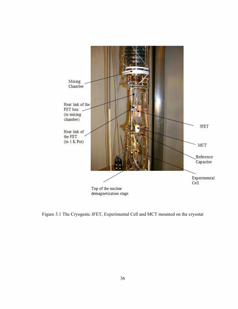
remained. This allowed us to install a cryogenic JFET pre-amplifier with operating

temperatures near 1 K in such a way that its physical location was near the sample cell

(see Figure 3.1).

36

Figure 3.1 The Cryogenic JFET, Experimental Cell and MCT mounted on the cryostat

37

Figure 3.2 Experimental Cell. (Built by D. Rosenberg) [33]

38

The JFET was thermally anchored to the 1 K pot using a silver wire of 0.06” in

diameter. Silver was annealed to improve its residual resistivity ratio. A thick-walled

copper box was surrounding the FET to prevent the heat radiated by the FET from

affecting the refrigerator. The box was thermally anchored to the mixing chamber using a

silver wire of 0.125” in diameter. Up to 2 mW of heat had to constantly be supplied to

keep the FET at an operational temperature. As a downside, it created additional

challenges in proper thermal management of the apparatus.

The experimental cell is mounted by clamping it to the top of the copper nuclear

demagnetization stage, which is described in detail in [32]. (Figure 3.2).

The nuclear demagnetization magnet with superconducting switch (built by

AMI Inc.) is capable of providing the magnetic field strength of 8 T. Applied to the

nuclear stage containing 154 moles of copper (bundle of wires), it allowed us to stay as

cold as 3-5 milliKelvin for several days in a row. We used nuclear demagnetization of

copper spins to control the temperature in this experiment. All the data in the range

between 2 and 30 mK were taken with help of nuclear demagnetization stage, with the

cell thermally connected to the nuclear stage and thermally disconnected from the

dilution unit. We found that the temperature stability was much better when the dilution

unit was thermally disconnected from demagnetization stage and cell. Therefore, we took

as much data as possible in that configuration. Temperatures in the range between 20 mK

and 100 mK were accessible by using the dilution unit. Thus, we were able to cover wide

39

range of temperatures. In addition, we had a possibility of controlling the temperature

with the Lakeshore conductance bridge, but since the demag setup provided enough

control over the temperature, it was not used.

The demagnetization magnet has compensation coils to ensure that the magnetic

field is minimal outside of the magnet bore. However, we still had a concern that demag

field might affect the measurements. Since the magnetic field effect on the dielectric

constant in the main focus of this work, we wanted to make sure that our results are not

affected by stray fields like the possible fringing fields from the nuclear demagnetization

stage. We’ve taken and compared the measurements at the same temperature, on the

same sample, with the same excitation voltage (drive field) values at different values of

current in the magnetization magnet, and it appeared that demag field strength had no

effect on the results of the experiment. The compensation coils are sufficient to not

concern ourselves with the fringe effects from the nuclear stage.

3.03 EXPERIMENTAL CELL

The ³He immersion cell was constructed from bronze by D. Rosenberg [33]. The

cell was bolted directly to the demagnetization stage of the refrigerator. The material of

the cell, on one hand, posed limitations on how quickly we were able to change the

magnetic field, but on the other hand allowed for shorter relaxation times. The cell was

mindfully constructed to keep the relaxation times as short as possible by minimizing the

volume of liquid ³He and by using a system of heat exchangers. The cell had a sintered

40

silver heat exchanger to provide good thermal contact of the ³He with the nuclear stage.

In addition, a set of two miniature heat exchangers was attached to each electrical lead to

provide the cooling of the samples. Samples are cooled through the leads. The gold plates

of electrodes also served as heat exchangers for the samples connected through short

copper leads to miniature sintered silver heat exchangers with an effective surface of

roughly 1 m². The heat sinks as well as the samples were immersed in liquid ³He.

Because the thermal conductivity of liquid ³He is comparable to that of copper at the

temperature of T ~10 mK, the main thermal resistance outside the sample is given by the

Kapitza resistance between helium and the silver surface as well as the boundary

resistance between the capacitor plates and the sample surfaces. The electrical leads were

separately heat sunk by sintered silver heat exchangers also inside the cell and then

connected by superconducting thin leads to the sample heat exchangers. This method,

developed by S. Rogge [29] ensures that the heat coming down on the leads from room

temperature or generated in the sample is effectively shunted to the liquid.

3.04 MAGNET

The magnet used to induce magnetic field in this experiment was a hand-wound

Helmholtz pair consisting of 300 loops each. Wire: Supercon VSF composite, 400

filaments, Ø = 0.0082”. L = 17.4 mH, Field to Current Ratio is 1.72 (±0.05) mT per Amp.

We could get to the maximum field of 30 mT without significantly boiling the bath. The

magnet was powered by a Kepco BOP 20-20M power supply which was driven by an

SRS DS345 Function generator.

41

Even though we believe that the material of the cell was somewhat limiting to

the speed at which we could change the magnetic field, we were just as limited by the

location of this magnet relative to the dilution unit. When we attempted field changes

faster than 3 µT/s , we saw that the performance of the dilution unit was affected to an

unacceptable degree even before we saw significant changes in the cell temperature. Note

that the cell temperature was measured by ³He melting curve thermometer (MCT) which

was thermally linked to the cell yet it was a physically separate and very small volume of

³He. Thus, the MCT itself was prone to Eddy currents as well. It’s not the cell that was

limiting the speed of the magnetic field changes but the placement and the geometry of

the magnet. The fact that the magnet didn’t allow for the superconducting mode and had

to be constantly powered also posed some limitations. For example, if we wanted to keep

the magnetic field at some constant value for an extended period of time, it would have

been nice to have the superconducting mode available. Instead, we had to “emulate” the

constant magnetic field by setting the function generator to 510 Hz, the lowest frequency

value that it could produce.

3.05 BRIDGE MEASUREMENT

Capacitance was measured using a standard analog bridge with a ratio

transformer, an ideal version of which is shown in Figure 3.3. For simplicity, only

reactive elements are shown, but a more realistic version should include resistive

elements as well. A good review of capacitance measurement is available in Appendix C

42

in [32]. The tap of the ratio transformer is grounded and can be moved until the signal VA

is nulled. When VA = 0, the following relation is satisfied:

1

sample

ref

Cx

x C (3.1)

Figure 3.3 Idealized representation of a variable ratio capacitance bridge, with sample

capacitance Csample and reference capacitance Cref

This allows us to learn the unknown capacitance directly. Of course, rather than

rebalancing the bridge continually, most actual measurements are taken by watching the

off-balance voltage between A and B, and relating it back to an effective change in x that

would be required to rebalance. That is, after balancing the bridge, we calibrate the

sensitivity of the bridge by changing x by a known amount ∆x, and measuring the

Csample

Cref “A”

“B”

43

resulting off-balance voltage ∆V. For small off-balance signals obV , we can now

approximate the effective / ( / )obx V V x . For small δx, we find

2(1 )

(1 )

sample ref

sample

sample

xC C

x

C x

C x x

(3.2)

A new reference capacitor was installed for this experiment that turned out to be

a good choice. The reference capacitor is a sapphire slab with the dimensions 0.374” x

0.354” x 0.035 with evaporated titanium-gold electrode plates. The reference capacitor is

physically located and thermally anchored to the sample plate of the apparatus. (Figure

3.1) 50.23refC pF at room temperature and 49.54refC pF at 4 K which demonstrates

the difference of only 1.37% over the range of 269 K. As it is widely known, the most

thermal contraction in solids usually occurs between room temperature and liquid helium

temperature and not as much at temperatures below 4 K. Our setup didn’t allow us to

measure refC directly at operating temperatures, but it is reasonable to assume that

refC didn’t change significantly between 2 mK and 100 mK where all our measurements

took place. When deciding on a placement of the reference capacitor, one usually wants

to put it in a temperature-stabilized environment. For example, it could be placed in a

vessel filled with liquid nitrogen, or it can be attached to 1 K pot of the dilution

refrigerator. We chose to put the reference capacitor at the sample plate. While the

temperature of the sample plate varies as we vary the temperature of the experimental

44

cell, these variations are insignificant in terms of change in capacitance as was stated

earlier. However, it significantly reduces the length of the coaxial cable between refC and

sampleC . Appendix A describes further details of the real bridge setup.

45

CHAPTER 4.

MEASUREMENT AND OBSERVATIONS

This chapter presents experimental data on the behavior of BK7, Aluminum-

Barium-Silicate, Suprasil, Corning microscope cover glass and Mylar film samples [21-

25] in the temperature range from 2 mK to 100 mK in the presence of a slowly varying

magnetic field. We measured the real part of the dielectric constant with the AC bridge

setup described in Chapter 3. The frequency of the AC electric field used in this

measurement is equal to 1 kHz throughout this work, unless specified otherwise. We

observed hysteresis in the dielectric response to a magnetic field varying in a saw-like

pattern with field strengths up to 1.8 milliTesla. Hysteresis happens in a narrow range of

temperatures and a narrow range of magnetic field, and it is highly correlated with the

excitation voltage (the magnitude of the AC drive field) on the sample. The pattern of the

response differs, depending on the glass composition.

4.01 ALUMINUM-BARIUM-SILICATE.

As first noted in [13], the dielectric constant of Aluminum-Barium-Silicate glass

(AlBaSi for short) displays an interesting tendency to “follow” the slowly varying

magnetic field. Figure 2.7 from [13] shows the variation in the magnetic field and the

corresponding response at 5.6 mK. We reproduced a similar measurement. (Figure 4.1)

This measurement is taken with the same magnetic field strength of 15 µT and an

excitation voltage of 4.5 kV/m as it was done in [13] and they are in good

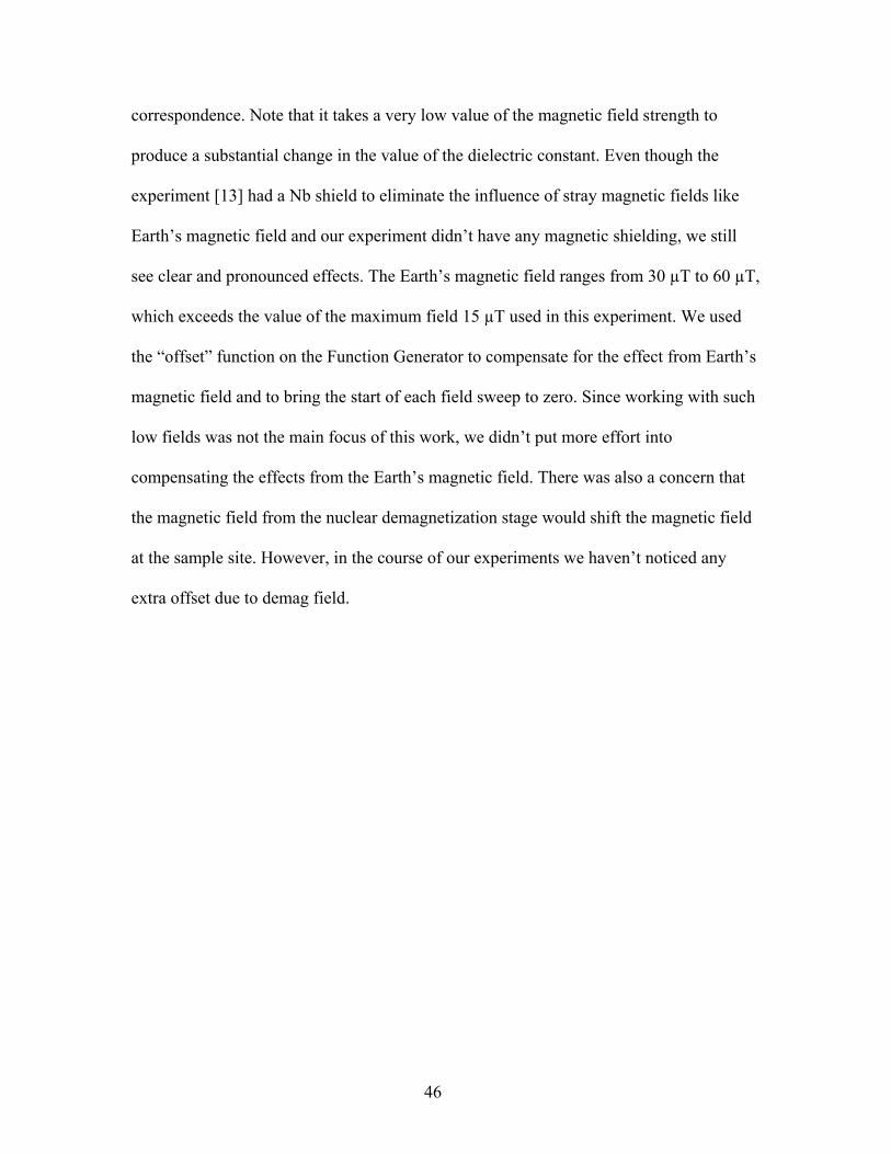
46

correspondence. Note that it takes a very low value of the magnetic field strength to

produce a substantial change in the value of the dielectric constant. Even though the

experiment [13] had a Nb shield to eliminate the influence of stray magnetic fields like

Earth’s magnetic field and our experiment didn’t have any magnetic shielding, we still

see clear and pronounced effects. The Earth’s magnetic field ranges from 30 µT to 60 µT,

which exceeds the value of the maximum field 15 µT used in this experiment. We used

the “offset” function on the Function Generator to compensate for the effect from Earth’s

magnetic field and to bring the start of each field sweep to zero. Since working with such

low fields was not the main focus of this work, we didn’t put more effort into

compensating the effects from the Earth’s magnetic field. There was also a concern that

the magnetic field from the nuclear demagnetization stage would shift the magnetic field

at the sample site. However, in the course of our experiments we haven’t noticed any

extra offset due to demag field.

47

Figure 4.1. Small Magnetic Field, AlBaSi, E = 4.5 kV/m, T = 5.6 mK.

The magnetic field strength and the electric field were chosen

the same as in [13]. This result is in good agreement with [13].

Magnetic Field Strength vs Time

-0.02

-0.015

-0.01

-0.005

0

0.005

0.01

0.015

0.02

0 10 20 30 40 50

Time, min

B, m

T

-8.00E-06

-6.00E-06

-4.00E-06

-2.00E-06

0.00E+00

2.00E-06

4.00E-06

0 10 20 30 40 50

Time, min

∆ε/ε

48

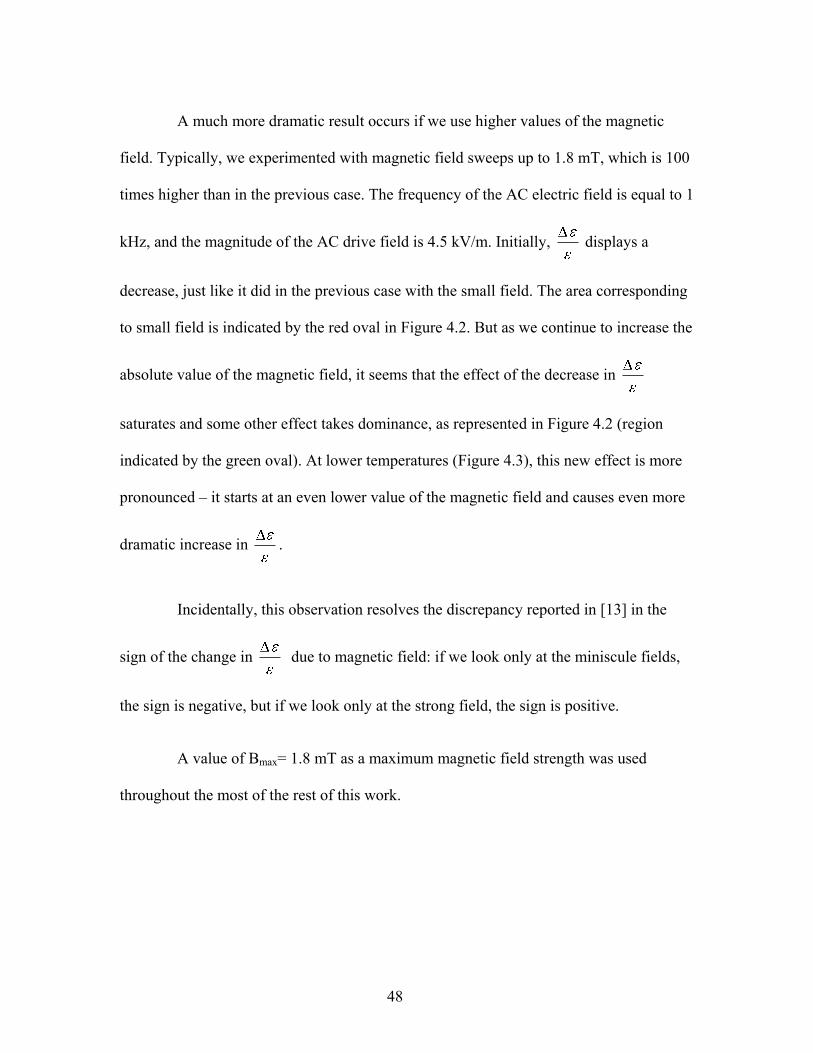
A much more dramatic result occurs if we use higher values of the magnetic

field. Typically, we experimented with magnetic field sweeps up to 1.8 mT, which is 100

times higher than in the previous case. The frequency of the AC electric field is equal to 1

kHz, and the magnitude of the AC drive field is 4.5 kV/m. Initially, displays a

decrease, just like it did in the previous case with the small field. The area corresponding

to small field is indicated by the red oval in Figure 4.2. But as we continue to increase the

absolute value of the magnetic field, it seems that the effect of the decrease in

saturates and some other effect takes dominance, as represented in Figure 4.2 (region

indicated by the green oval). At lower temperatures (Figure 4.3), this new effect is more

pronounced – it starts at an even lower value of the magnetic field and causes even more

dramatic increase in .

Incidentally, this observation resolves the discrepancy reported in [13] in the

sign of the change in due to magnetic field: if we look only at the miniscule fields,

the sign is negative, but if we look only at the strong field, the sign is positive.

A value of Bmax= 1.8 mT as a maximum magnetic field strength was used

throughout the most of the rest of this work.

49

Figure 4.2 Typical Magnetic Field Sweep, AlBaSi, E = 4.5 kV/m, T = 5.6 mK.

The electric field was chosen the same as in [13]. The magnetic

field strength was 100 times higher than in [13] and in Figure

4.1 The result is still consistent with [13] and with Figure 4.1 in

the area shown by the red oval, but it displays new behavior as

the magnitude of the B field increases.

-2

-1.5

-1

-0.5

0

0.5

1

1.5

2

0 10 20 30 40 50

Time, min

B, m

T

-2.50E-05

-2.00E-05

-1.50E-05

-1.00E-05

-5.00E-06

0.00E+00

5.00E-06

0 10 20 30 40 50

Time, min

∆ε/ε

50

Figure 4.3 Magnetic Field Sweep, AlBaSi, E = 4.5 kV/m, T = 1.47 mK.

The frequency and the magnitude of the AC drive field was chosen the

same as in [13]. The magnetic field strength was 100 times higher than

in [13] and in Figure 4.1. We’ve noticed that in a certain region of

temperatures for this sample ∆ε/ε shows a decrease, and then an

increase in the response to the magnetic field. This was unexpected.

-2

-1.5

-1

-0.5

0

0.5

1

1.5

2

0 10 20 30 40 50 60 70

Time, min

B,

mT

-5.00E-06

0.00E+00

5.00E-06

1.00E-05

1.50E-05

2.00E-05

0 10 20 30 40 50 60 70

Time, min

∆ε/ε

51

4.02 SUPRASIL, MYLAR

We applied similar test conditions Suprasil and Mylar. That is, we applied

slowly varying magnetic field with the amplitude of 1.8 mT to a slab of material while

measuring its dielectric response. (See Figure 4.3 for the pattern of the applied magnetic

field.) The amplitude of the AC electric field used in this measurement was chosen close

to that on AlBaSi experiments We saw no effect at several temperature points. That is,

vs B (or vs time) is essentially a straight horizontal line, if we disregard the

noise and temperature drift (Figure 4.4 and Figure 4.5). The temperature drift, which is

especially noticeable in Mylar, is due to the fact that this temperature range is accessible

with the nuclear demagnetization stage, and when the data is taken long after demag, the

cooling ability (incorrectly but frequently referred to as cooling entropy in ultra low

temperature jargon) is mostly lost, and the temperature change due to heat leak over 44

minute interval becomes noticeable.

The results of testing Suprasil and Mylar are two-fold: first of all, we convince

ourselves that the observed effect is due to magnetic field and not due to heating.

Otherwise, if the effect were due to heating, we’d see it in all samples since we treat all

samples identically in terms of experiment. Second, we note that some glasses are

insensitive to magnetic fields. Incidentally, Mylar and Suprasil have (a) different

composition in terms of presence of nuclear spins and (b) display different behavior in

versus T at temperatures below 5 mK. They have no plateau region at low

temperatures.

52

We had an interest in experimenting with Mylar because it is unusual in a sense

that its dielectric response doesn’t behave the same way as that of the most other known

glasses. Below and above the temperature of the minimum the capacitance depends

logarithmically on temperature with a slope ratio of : 2 :1low highS S for most glasses.

For Mylar, this ratio is between -2:1 and -2:2 [34]. Even though the deviation is seen

only above the minimum in capacitance, where magnetic field effect is not observed, it

-3.00E-06

-2.50E-06

-2.00E-06

-1.50E-06

-1.00E-06

-5.00E-07

0.00E+00

0 10 20 30 40 50

Time, min

Figure 4.4 Suprasil, E = 3.9 kV/m, T = 5.8 mK

The magnetic field was applied to the sample and changed in

the same saw-like pattern in the same manner as it was done

for AlBaSi. We don’t see any dependence on the magnetic

field, only the temperature drift.

53

-2.50E-06

-2.00E-06

-1.50E-06

-1.00E-06

-5.00E-07

0.00E+00

5.00E-07

1.00E-06

0 10 20 30 40 50

Time, min

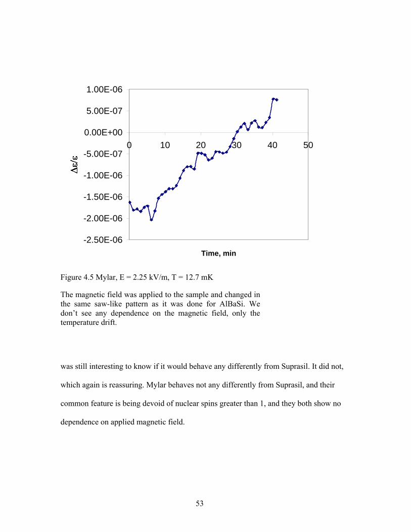
Figure 4.5 Mylar, E = 2.25 kV/m, T = 12.7 mK

The magnetic field was applied to the sample and changed in

the same saw-like pattern as it was done for AlBaSi. We

don’t see any dependence on the magnetic field, only the

temperature drift.

was still interesting to know if it would behave any differently from Suprasil. It did not,

which again is reassuring. Mylar behaves not any differently from Suprasil, and their

common feature is being devoid of nuclear spins greater than 1, and they both show no

dependence on applied magnetic field.

54

4.03 HYSTERESIS ON ALBASI

It is interesting to observe what happens if we plot versus applied magnetic

field. Figure 4.6 shows the same data as Figure 4.2 where “time” was eliminated. In the

similar fashion, Figure 4.7 shows the same data as Figure 4.3 where “time” was

eliminated. The sweep starts at B = 0. Colors and arrows are to help the reader map the

branches of the hysteresis to the corresponding parts of the magnetic field sweep. We

notice rather strong hysteresis. The sweep can be done either way – negative part first or

positive part first. In fact, it is impossible to tell from the Figure 4.6 or Figure 4.7 which

way did the magnetic field was initially changed. We also didn’t see any difference

experimentally. In addition, Figure 4.7 demonstrates what happens if we plot more than

one period of the magnetic field. Figure 4.8 and Figure 4.9 show the family of such

curves for different temperatures at a fixed drive field value of E = 4.5 kV/m. Two

separate plots were used to show it in order to avoid over-crowding. Figure 4.13 and

Figure 4.14 show a similar family of curves for the drive field value of E = 2.25 kV/m.

It is natural to ask if the hysteresis is still present if we were to vary the field

more slowly. We tried sweeping the field at four times slower rate (0.73 µT/s); the

hysteresis is still present, but the area of the hysteresis loop is smaller. Varying the field

much slower than 0.73 µT/s was difficult as such sweeps would take more than 3 hours.

55

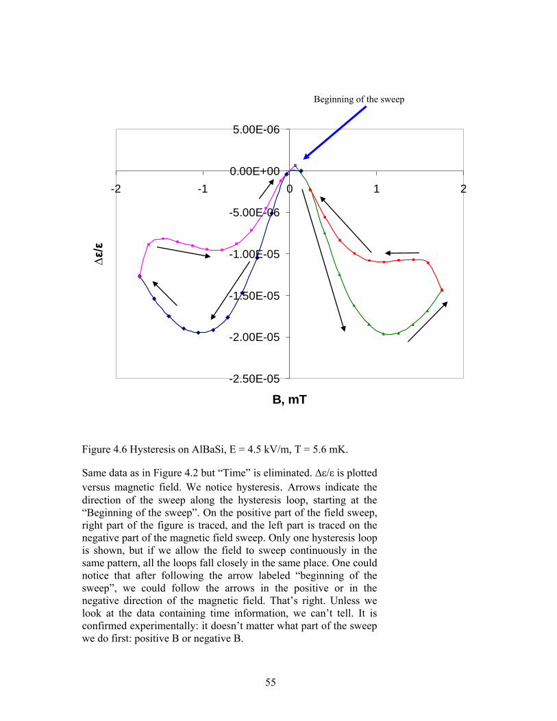
Figure 4.6 Hysteresis on AlBaSi, E = 4.5 kV/m, T = 5.6 mK.

Same data as in Figure 4.2 but “Time” is eliminated. ∆ε/ε is plotted

versus magnetic field. We notice hysteresis. Arrows indicate the

direction of the sweep along the hysteresis loop, starting at the

“Beginning of the sweep”. On the positive part of the field sweep,

right part of the figure is traced, and the left part is traced on the

negative part of the magnetic field sweep. Only one hysteresis loop

is shown, but if we allow the field to sweep continuously in the

same pattern, all the loops fall closely in the same place. One could

notice that after following the arrow labeled “beginning of the

sweep”, we could follow the arrows in the positive or in the

negative direction of the magnetic field. That’s right. Unless we

look at the data containing time information, we can’t tell. It is

confirmed experimentally: it doesn’t matter what part of the sweep

we do first: positive B or negative B.

Beginning of the sweep

-2.50E-05

-2.00E-05

-1.50E-05

-1.00E-05

-5.00E-06

0.00E+00

5.00E-06

-2 -1 0 1 2

B, mT

∆ε/ε

56

Figure 4.7 Hysteresis on AlBaSi, E = 4.5 kV/m, T = 1.47 mK.

Same data as in Figure 4.3 but “Time” is eliminated. ∆ε/ε is

plotted versus magnetic field. We notice hysteresis as well,

even though it is much less pronounced at this low

temperature.

-5.00E-06

0.00E+00

5.00E-06

1.00E-05

1.50E-05

2.00E-05

-2 -1 0 1 2

B, mT

57

-2.00E-05

-1.50E-05

-1.00E-05

-5.00E-06

0.00E+00

5.00E-06

1.00E-05

1.50E-05

2.00E-05

-2 -1 0 1 2

B, mT

3.35 mK

2.32 mK

1.47 mk

Figure 4.8 AlBaSi Hysteresis Loops, Very Low Temperatures, E = 4.5 kV/m

58

-2.50E-05

-2.00E-05

-1.50E-05

-1.00E-05

-5.00E-06

0.00E+00

5.00E-06

-2 -1 0 1 2

B, mT

31.5 mK

24.7 mK

14.5 mK

12.0 mK

5.16 mK

Figure 4.9 AlBaSi Hysteresis Loops, Intermediate Temperatures, E = 4.5 kV/m

At the level of the drive field E = 4.5 kV/m, we observe

hysteresis for the whole range of temperatures up to 30 mK. It

disappears as higher temperature (not shown, but data is

available). Also, we note the initial decrease in the ∆ε/ε (also

see Figure 4.8).

59

-2.50E-05

-2.00E-05

-1.50E-05

-1.00E-05

-5.00E-06

0.00E+00

5.00E-06

1.00E-05

1.50E-05

2.00E-05

-2 -1 0 1 2

B, mT

8.9 mK, E = 240 V/M

8.9 mK, E = 640 V/M

8.9 mK, E = 1320 V/M

8.6 mK, E = 4500 V/M

12.3 mK, E = 2250 V/M

Figure 4.10 Role of the Excitation Voltage / Drive Fields in the Dielectric

Response of AlBaSi Sample.

Hysteresis takes place for all values of the drive field Edrive .

(See also Figure 4.11.) For E = 4.5 kV/M the initial decrease

in ∆ε/ε is particularly significant which makes us question the

linearity of the measurement regime at this value of Edrive

Negative change in ∆ε/ε at the start of the sweep begins at as

low of a value for the drive field as Edrive= 1.32 kV/m.

60

-5.00E-07

0.00E+00

5.00E-07

1.00E-06

1.50E-06

2.00E-06

2.50E-06

3.00E-06

3.50E-06

4.00E-06

-2 -1 0 1 2B, mT

8.9 mK, E = 240 V/M

8.9 mK, E = 640 V/M

8.9 mK, E = 1320 V/M

Figure 4.11 Role of the Excitation Voltage / Drive Fields in the Dielectric

Response of AlBaSi Sample, low excitation voltages.

This figure illustrates the point that hysteresis takes place even

at lowest levels of the drive field.

61

Figure 4.12 Typical picture of ∆ε/ε vs B, with hysteresis, AlBaSi, E = 2.25 kV/m,

T = 4.15 mK.

Arrows indicate the direction of the sweep along the hysteresis loop, starting at the

“Beginning of the sweep”. On the positive part of the field sweep, right part of the

figure is traced, and the left part is traced on the negative part of the magnetic field

sweep. Again, as in Figure 4.6, one could notice that after following the arrow

labeled “beginning of the sweep”, we could follow the arrows in the positive or in

the negative direction of the magnetic field. If we didn’t have the top graph, we

couldn’t tell which way did the B filed change – positive or negative.

-2

-1.5

-1

-0.5

0

0.5

1

1.5

2

2.5

0 10 20 30 40 50

Time, min

B,

mT

-2.00E-06

0.00E+00

2.00E-06

4.00E-06

6.00E-06

8.00E-06

1.00E-05

1.20E-05

1.40E-05

1.60E-05

-2 -1 0 1 2 3

B, mT

∆ε/ε

beginning

62

-1.00E-05

0.00E+00

1.00E-05

2.00E-05

3.00E-05

4.00E-05

5.00E-05

-2 -1 0 1 2

B, mT

12.3 mK

4.15 mK

2.3 mK

1.7 mK

Figure 4.13 AlBaSi hysteresis curves, various temperatures, E = 2.25 kV/m.

The overall influence of magnetic fields is stronger at low

temperatures. Hysteresis is less pronounced at this lower value

of the drive field, as compared to E = 4.5 kV/m, as well as the

initial drop in ∆ε/ε.

63

-5.00E-06

0.00E+00

5.00E-06

1.00E-05

1.50E-05

2.00E-05

2.50E-05

3.00E-05

3.50E-05

4.00E-05

4.50E-05

-2 -1 0 1 2 3

B, mT

30.5 mK

17.6 mK

14.75 mK

Figure 4.14 AlBaSi Hysteresis Loops, Higher Temperatures, E = 2.25 kV/m

It has been mentioned in the literature [17] that the magnetic field effect is

dependent on the strength of the driving field, but without much detail. We experimented

at T ~ 10 mK with different drive fields stepping down its value as low as the noise in the

experiment had allowed us to go. (Figure 4.10 and Figure 4.11) Hysteresis takes place for

64

all values of the drive field, including the lowest value E = 240 V/m. For E = 4.5 kV/m

the initial decrease in is particularly significant and the overall shape of the effect

looks rather different which makes us believe that the measurements at the value of

driveE = 4.5 kV/m are non-linear for temperatures of 10 mK (and lower). driveE = 2.25

kV/m seems to be a better value of the drive field to work with than driveE = 4.5 kV/m,

although the hysteresis effect seems to be inherently non-linear. The effect of the initial

drop in is present at all values of the drive field; however, with lower values of the

drive field this effect covers narrower ranges of temperatures: with driveE = 4.5 kV/m it is

quite profound everywhere below 30 mK, while if we decrease the value of the driving

field by a factor of 2 ( driveE = 2.25 kV/m) this effect is only seen in the range

4.15mK T 14.75mK .

The overall influence of magnetic fields is more profound at low temperatures,

in the sense that it produces greater overall change in . The region

4.15mK T 14.75mK is special as it displays the initial drop in and strong

hysteresis. If we calculate areas surrounded by each hysteresis loop and then plot it with

respect to temperature we see an interesting result (Figure 4.15). The curves have the

maximum near 5-7 mK. It is expected to see a maximum in response when the energy of

the two level systems responsible for the phenomenon corresponds to the temperature.

Said temperature 5-7 mK is of the order of energy of quadrupoles interacting with the

65

two level systems. So it is quite plausible to see the maximum in *B versus

temperature near 5-7 mK. It is also in good correspondence with the theoretical research

[41]. Theoretical prediction for temperature dependence of the contribution to the

permittivity of tunneling systems due to quadrupole interaction is shown in Figure 2.10 .

Figure 4.15 Area of hysteresis loops, AlBaSi.

Each point on this graph represents the area of a hysteresis loop

from the families of curves for different temperatures and drive

field values shown in Figure 4.8, Figure 4.9 and Figure 4.13,

Figure 4.14. This result is interesting to compare to the results

from [41] “Temperature dependence of the contribution to the

permittivity of tunneling systems due to the quadrupole

interaction” shown in Figure 2.10

0.00E+00

2.00E-06

4.00E-06

6.00E-06

8.00E-06

1.00E-05

1.20E-05

0 10 20 30 40

T, mK

* B

, m

T

2.25 kV/m

4.5 kV/m

66

4.04 BK7

We performed similar measurements of the resonant dielectric constant under

the application of a magnetic field varying in a saw-like pattern on BK7. Figure 4.16 and

Figure 4.17 show a typical result. The magnitudes of the drive field were deliberately

chosen close to that used on AlBaSi. We were also hoping to stay in the linear regime for

all temperatures. Based on the previous work in the field [29], BK7 responds linearly to

drive fields of the order of 1 kV/m and in the temperatures of 10 mK and above. In the

example shown in Figure 4.16 and Figure 4.17 driveE = 2.14 kV/m and T = 4.6 mK. Figure

4.18 shows what happens at other temperatures. Like in the case of AlBaSi, we note the

region of temperatures with strong hysteresis. We observe magnetic field dependence

with hysteresis in the following range of temperatures T < 10 mK for E = 2.14 kV/m and

T < 12 mK for E = 4.28 kV/m. Generally, we observe magnetic field dependence in BK7

below T = 50 mK.

The most striking difference of BK7 from AlBaSi (and from Corning, as we will see

later) is that for BK7 did not show a decrease at the start of the field sweep like it did

for AlBaSi. Neither did it show a decrease when we tested higher excitation voltages.

Results for driveE = 4.28 kV/m are shown in Figure 4.19.

It might be worth noting that the maximum magnetic field changes non-

monotonically with temperature (Figure 4.20)

67

Figure 4.16 Typical sweep of magnetic field on BK7, E = 2.14 kV/m, T = 4.6 mK.

Unlike AlBaSi, BK7 demonstrates hardly any initial drop in ∆ε/ε.

-2

-1.5

-1

-0.5

0

0.5

1

1.5

2

0 10 20 30 40 50

Time, min

B, m

T

0.00E+00

1.00E-06

2.00E-06

3.00E-06

4.00E-06

5.00E-06

6.00E-06

0 10 20 30 40 50

Time, min

∆ε/ε

68

Figure 4.17 Typical sweep of magnetic field on BK7: hysteresis, E = 2.14 kV/m, T = 4.6

mK.

Same data as in Figure 4.16 but “Time” is eliminated. ∆ε/ε is

plotted versus magnetic field. We notice hysteresis.

0.00E+00

1.00E-06

2.00E-06

3.00E-06

4.00E-06

5.00E-06

6.00E-06

-2 -1 0 1 2

Time, min

69

Figure 4.18 BK7 Hysteresis Loops, Various Temperatures, E = 2.14 kV/m.

Note non-monotonous dependence of the maximum values on

temperatures. Region T < 13 mK has additional non-

monotonous effects.

0.00E+00

2.00E-06

4.00E-06

6.00E-06

8.00E-06

1.00E-05

1.20E-05

1.40E-05

1.60E-05

1.80E-05

2.00E-05

-2 -1 0 1 2Magnetic Field, mT

∆ε/ε

1.86 mK

2.49 mK

4.59 mK

0.00E+00

5.00E-06

1.00E-05

1.50E-05

2.00E-05

2.50E-05

-2 -1 0 1 2

Magnetic Field, mT

∆ε/ε

12.07 mK

13.08 mK

20.0 mK

32.5 mK

99.6 mK

70

Figure 4.19 BK7 hysteresis loops, various temperatures, E = 4.28 kV/m.

Note non-monotonous dependence of the maximum values on

temperature.

-2.00E-06

0.00E+00

2.00E-06

4.00E-06

6.00E-06

8.00E-06

1.00E-05

1.20E-05

-2 -1 0 1 2 3

B, mT

∆ε/ε

4.56 mK

6.85 mK

7.77 mK

9.82 mK

11.41 mK

12.3 mK

-2.00E-06

0.00E+00

2.00E-06

4.00E-06

6.00E-06

8.00E-06

1.00E-05

1.20E-05

-2 -1 0 1 2 3

B, mT

∆ε/ε

12.3 mK

19.8 mK

23.85 mK

33.2 mK

56.5 mK

99.6 mK

71

Figure 4.20 Maximum change in dielectric constant due to applied field or 1.8 mT at

different temperatures.

0.00E+00

5.00E-06

1.00E-05

1.50E-05

2.00E-05

2.50E-05

0 20 40 60 80 100 120

T, mK

max v

alu

es E = 2.14 kV/m

E = 4.28 kV/m

72

4.05 CORNING

We performed similar measurements of the resonant dielectric constant under

application of a magnetic field varying in a saw-like pattern on Corning glass. Figure

4.21 shows typical results. The magnitudes of the drive field were deliberately chosen

close to that used on AlBaSi and BK7. We were also hoping to stay in the linear regime

for all temperatures. In this example driveE = 2.14 kV/m. As we see, the overall behavior is

similar to that of AlBaSi. Initially, as soon as we start increasing the magnetic field from

zero, we see a decline of , which soon changes to a rise. The overall shape of

hysteresis is also similar to that of AlBaSi.

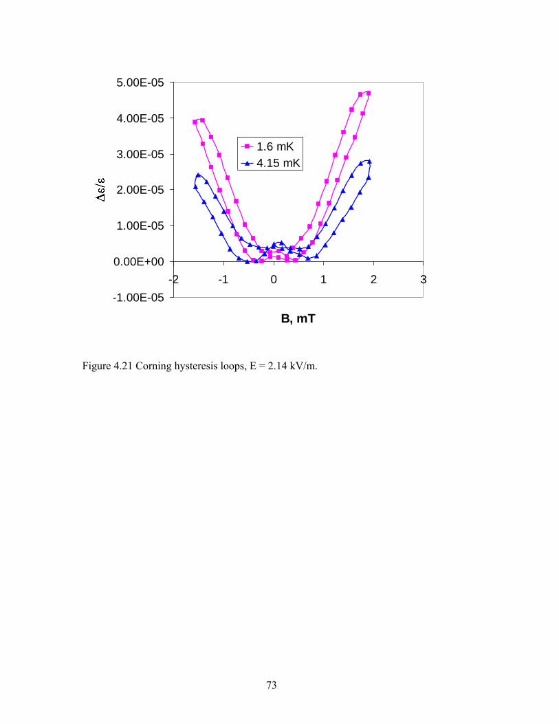
73

Figure 4.21 Corning hysteresis loops, E = 2.14 kV/m.

-1.00E-05

0.00E+00

1.00E-05

2.00E-05

3.00E-05

4.00E-05

5.00E-05

-2 -1 0 1 2 3

B, mT

1.6 mK

4.15 mK

74

CHAPTER 5.

DISCUSSION

The observed response of the dielectric constant to a swept magnetic field is

clearly correlated with a glass composition. As we can see from Table 5.1, BK7 contains

nuclear spins I = 3/2 due to barium, sodium, potassium and boron; BaO-Al2O3-SiO2

contains I = 3/2 due to barium and I = 5/2 due to aluminum. Corning contains I = 5/2 due

to magnesium and aluminum. These three glasses containing nuclei with nuclear spin

greater than ½ display the dependence of the diectric constant on applied magnetic field.

On the other hand, Mylar and Suprasil don’t contain nuclear spins greater than ½, and

they don’t show any response to magnetic fields and don’t display the deviation from

logarithmic behavior at low temperatures as was mentioned in Chapter 2. This supports

the suggested origin of both phenomena as being due to the presence of nuclear spins 3/2

and greater.

Another good question is why the pattern of response of BK7 is different than

that of AlBaSi or Corning. To put it differently, one could ask why does the dielectric

constant decrease (in cases of AlBaSi and Corning) at all when we apply a magnetic field

to the glass. According to the existing theory [20], nuclear quadrupole contribution

restores coherent tunneling, therefore the expected behavior for the dielectric constant at

77

Glass Components Effect

observed?

Nuclear

spin

Suprasil SiO2 No Si: I = ½

O: I = 0

AlBaSi

(barium

aluminosilicate)

BaO

(35.8%)

Al2O3

(26.8%)

SiO2

(35.1%)

K2O (2.3%)

Yes Ba: I = 3/2

Al: I = 5/2

K: 3/2

BK7 SiO2 64%

B2O3 15%

BaO 6%

Na2O 7%

K2O 5%

Yes Ba: I = 3/2

Na: 3/2

K: 3/2

B: 3/2

(80%

abundance)

Corning SiO2 73%

Na2O 14%

CaO 7%

MgO 4%

Al2O3 2%

Yes Mg: 5/2

(10%

abundance)

Al: 5/2

Ca: I = 0

Na: 3/2

Mylar

(Polyethylene

terephthalate,

PETE)

C10H8O4 No O: I = 0

H: I = ½

C: I = 0

Table 5.1 Chemical composition of glass samples.

77

temperatures near 5 mK is to increase under the influence of the magnetic field. Nuclear

spins with I ≥ 1 should always result in an increase of at small field as pointed out by

[20]. The observed decrease must be due to some other effect. What special can happen

at a field of 1 mT and a temperature of 5 mK? One possibility, according to A. Burin

[44], is to consider the electronic spin associated with a tunneling entity in AlBaSi and

Corning.

At 1 mT magnetic field the Zeeman splitting of electronic spin is 1.8*2*µB ~

2mK, almost the thermal energy and g factor; or participation of more than one electron

can make things comparable. Of course the effect of electronic spins should be stronger

at lower temperatures. Therefore one possible suggestion is the effect of electronic spins.

A non-monotonic dependence can be related to the non-equilibrium effects

which are very difficult to interpret. In addition, according to Burin et al [35, 45] the

external magnetic field can restore the coherence of tunneling thus increasing the

dielectric constant. This effect can be seen when the Zeeman splitting becomes

comparable to the thermal energy.

77

CHAPTER 6. CONCLUSIONS AND FUTURE WORK.

We studied the dielectric response of five different amorphous materials (Table

5.1) below 100 mK in the presence of a slowly varying in a saw-like pattern weak

magnetic field. AC capacitive measurements were made at several different values of the

AC drive field, all of which were close to or lower than that used previously by other

researchers. We found the following: (a) the dielectric response of glasses containing

atoms with nuclear spins equal to and greater than 3/2 displays a dependence on applied

magnetic field; the dielectric response of glasses devoid of atoms with nuclear spins

smaller than 3/2 is independent of applied magnetic field; (b) hysteresis in the response to

a magnetic field in a certain range of temperatures, which depends on the glass

composition, on temperature and on the value of the drive field; (c) this effect is strongly

correlated with the strength of the AC electric (drive) field, even at very low levels. The

typical range of temperatures where hysteresis is observed is 5 mK < T < 15 mK.

Although our findings are consistent with the idea that nuclear spins are responsible for

the magnetic field effect, they are not fully explained by it. The difficulty of further

analysis of our data arises from the fact that we had many factors affecting the TLS at the

same time – changing magnetic field, AC measuring field, and on top of that, glasses are

known to have long relaxation times. It might be interesting to study relaxation behavior

– bring the magnetic field to a certain value and let it stay constant while observing the

77

dielectric response. Due to limitations of our setup, we were unable to produce constant

magnetic field which does not change its value over an extended period of time.

It would be interesting to study what happens if we were to use much higher

magnetic field at 5 mK and below. There is a prediction of coherent tunneling being

restored by the application of a high (~ 10 T) magnetic field, and most likely a rich

variety of phenomena would be found.

79

APPENDIX A:

CRYOGENIC JFET

The bridge measurement setup used a cryogenic JFET (Infrared Laboratories,

SST-U401 series) in a source follower configuration (Figure 6.1). The main difference

from the setup previously used is that the JFET is located near the sample plate (Figure

3.1) and thus physically close to the samples and reference capacitor, hence allowing for

shorter wires which in turn eliminates a large portion of capacitance to ground thus

enhancing signal to noise ratio. Note that the point of connection of sampleC , Gate and

refC is located inside the cryostat, which makes troubleshooting very inconvenient: when

apparatus is cold, there is no access to that important point. By moving this point inside

the fridge, we eliminated about two meters of coaxial wire at the expense of testing

convenience and flexibility. JFET is designed to work at 4 K. It was thermally anchored

to the 1 K pot with the FET box thermally anchored to the mixing chamber. The heat up

to 2 mW had to be constantly supplied to keep the FET operational. Note it is possible to

run the FET without any external power at the initial cool-down, but it is advised to start

heating it once the dilution unit is running.

After examining the diagram, one might argue that FET is not even necessary

for this measurement. But here are the reasons to use it. The unknown capacitor has large

impedance (100 pF at 1 kHz is equivalent to 100 M impedance). Lockin Amplifier has

79

small input impedance. Without the FET, we would be attempting to draw large currents

through the sampleC which in turn changes the voltage on sampleC which is what we are

trying to measure in the first place. With the FET, large current is diverted to 10M

resistor and we end up measuring a better signal.

Figure 6.1 Electronic measurement setup

Vex is provided by PAR-124A Lockin amplifier; f = 1 kHz for

most cases. Cryogenic JFET is in source follower configuration

with input impedance set to 10 M which is larger than

impedance to ground due to the coax in our frequency range.

Blue border is showing the parts that are cooled (located inside

IVC). Capacitance and resistance due to cables is not shown.

Csample

Cref

LA

81

APPENDIX B:

CAPACITANCE VERSUS TEMPERATURE, ZERO MAGNETIC FIELD

Although studying dielectric response in absence of a magnetic field was not the

main purpose of this work, such measurement serves as a good reference. Below we

include the result for AlBaSi sample.

131.4

131.45

131.5

131.55

131.6

131.65

131.7

1 10 100

T, mK

C, p

F

AlBaSi, 2.25 kV/m

AlBaSi, 4.5 kV/m

Figure 6.2 Capacitance vs temperature, AlBaSi.

82

APPENDIX C:

RELAXATION MEASUREMENTS

After consistently observing a hysteresis, it is rather natural to ask what happens

if we vary the magnetic field more slowly? We tried field sweeps on both AlBaSi and

BK7 which were 4 times slower than our typical measurement. That is, we varied the

magnetic field at 0.73 µT/s instead of our usual 2.9 µT/s. We picked the temperatures

where the hysteresis was the most pronounced – near 6 mK. Hysteresis was still present,

and the overall shape of the loop remained the same, although the area of the loop

reduced. Note that a sweep at this slower rate takes almost 3 hours. It was not uncommon

to experience temperature variations over this period of time due to various reasons,

which it turn would ruin the data set that’s currently being taken.

Another possibility was to stop the sweep at various points and observe the

dielectric response. One example of it is presented in Figure 6.3 and Figure 6.4, where

the sweep was stopped every 5 minutes and then allowed to continue for another 5

minutes. We see relaxation in ∆ε/ε every time we stop the sweep, but clearly it’s not

reaching its equilibrium values. We attempted another experiment, where we took care to

see that ∆ε/ε stops changing before we continue the sweep (Figure 6.5).

84

-2

-1.5

-1

-0.5

0

0.5

1

1.5

2

0 50 100

Time, min

B, m

T

-2.50E-05

-2.00E-05

-1.50E-05

-1.00E-05

-5.00E-06

0.00E+00

5.00E-06

0 20 40 60 80 100 120

Time, min

Figure 6.3 AlBaSi, E = 4.5 kV/m, T = 5.6 mK. Sweep in steps.

The sweep was stopped approximately every 5 minutes and

then allowed to continue. Top figure shows the pattern of

applied magnetic field. Bottom figure shows the dielectric

response.

84

-2.50E-05

-2.00E-05

-1.50E-05

-1.00E-05

-5.00E-06

0.00E+00

5.00E-06

-1.5 -1 -0.5 0 0.5 1 1.5

B, mT

Figure 6.4 AlBaSi, E = 4.5 kV/m, T = 5.6 mK. Sweep in steps, ∆ε/ε vs B

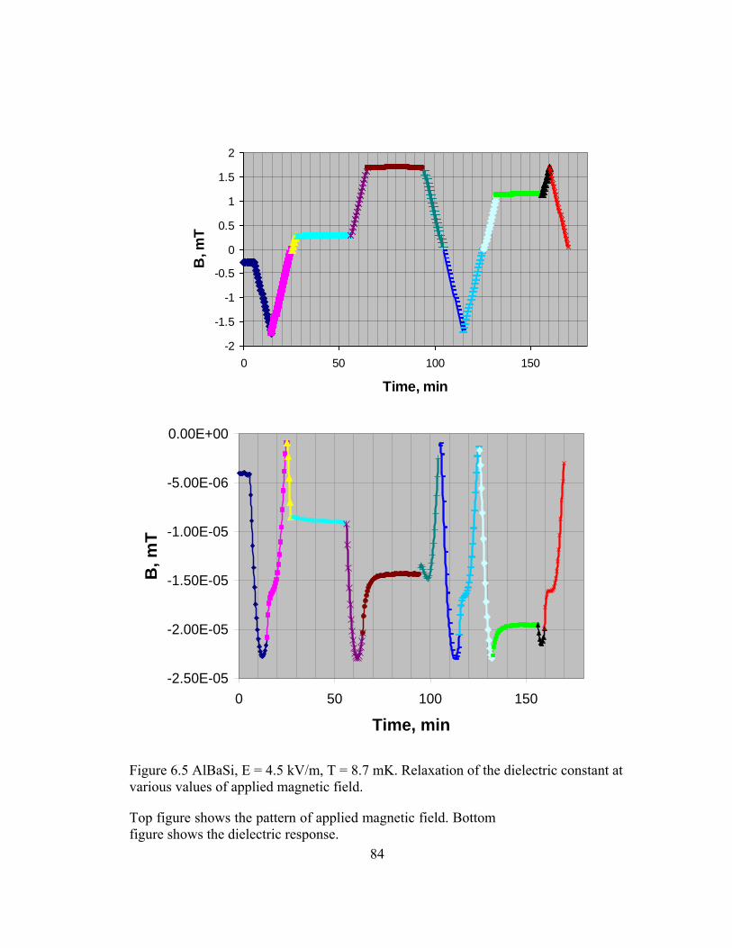
84

-2

-1.5

-1

-0.5

0

0.5

1

1.5

2

0 50 100 150

Time, min

B, m

T

-2.50E-05

-2.00E-05

-1.50E-05

-1.00E-05

-5.00E-06

0.00E+00

0 50 100 150

Time, min

B,

mT

Figure 6.5 AlBaSi, E = 4.5 kV/m, T = 8.7 mK. Relaxation of the dielectric constant at

various values of applied magnetic field.

Top figure shows the pattern of applied magnetic field. Bottom

figure shows the dielectric response.

86

BIBLIOGRAPHY

1. Anderson, P., B. Halperin, C. Varma. “Anomalous low temperature thermal

properties of glasses and spin glasses.” Phil. Mag., 25, pp.1-9 (1972)

2. Anthony, P.J., A.C. Anderson. “Frequency and temperature dependence of

dielectric and ultrasonic dispersion in amorphous materials at low temperatures.”

Phys. Rev. B. 20 (2), pp.763-767 (1979)

3. Phillips, W., editor. “Amorphous Solids.” Springer-Verlag, Berlin (1981)

4. Esquinazi, P., editor. “Tunneling Systems in Amorphous and Crystalline Solids.”

Springer, (1998)

5. Salvino, D., S. Rogge, B. Tigner, D.D. Osheroff. “Low temperature AC dielectric

response of glasses to high DC electric fields.” Phys. Rev. Lett. 73 (2), pp.268-271

(1994)

6. Stockburger, J. T., M. Grifoni, M. Sassetti. “Non-linear acoustic response of

glasses in the tunneling model.” Phys. Rev. B. 51 (5), pp2835-2843 (1995)

7. Burin, A. L. “Dipole gap effects in low energy excitation spectrum of amorphous

solids. Theory for dielectric relaxation.” J. Low Temp. Phys., 100 (3/4), pp.309-337

(1995)

8. Lasjaunas, J., R. Maynard, and M. Vandorpe. “Existence of a gap in the low

energy density of states in vitreous silica.” J. Phys., 39 (8), 973 (1978)

9. Yu, C and A. Leggett. “Low temperature properties of amorphous materials:

Through a glass darkly”. Comments Cond. Mat. Phys., 14 (4), 231 (1988).

10. Jäkle, J. “On the ultrasonic attenuation in glasses at low temperatures”. Z. Phys.,

257, 212 (1972)

11. Phillips, W. “Tunneling states in amorphous solids”. J. Low Temp. Phys., 7 ,

351, (1972).

12. Kittel, C. Introduction to Solid State Physics. Wiley, New York (1996).

87

13. Strehlow, P., C. Enss, S. Hunklinger. “Evidence for a phase transition in glasses

at very low temperature: a macroscopic quantum state of tunneling systems?” Phys.

Rev. Lett. 80 (24), pp.5361-5364 (1998)

14. Hunklinger, S., C. Enss, P. Strehlow. “Macroscopic quantum state of tunneling

systems.” Physica B 263-264 pp.248-252 (1999)

15. Hunklinger, S., C. Enss, P. Strehlow. “Quantum phenomena in glasses at low

temperatures.” Physica B 280 pp.271-275 (2000)

16. Strehlow, P., M. Wohlfahrt, A.G.M. Jansen, R. Hauesen, G. Weiss, C. Enss, S.

Hunklinger. “Magnetic Field dependent tunneling in glasses.” Phys. Rev. Lett. 84

(9), pp.1938-1941 (2000)

17. Wohlfahrt, M., P. Strehlow, C. Enss, S. Hunklinger. “Magnetic-field effects in

non-magnetic glasses.” Europhys. Lett., 56 (5), pp.690-694 (2001)

18. Ludwig, S., C. Enss, P. Strehlow, S. Hunklinger. “Direct coupling of magnetic

fields to tunneling systems in glasses.” Phys. Rev. Lett. 88 (7), 075501-1-4 (2002)

19. Enss, C. “Beyond the tunneling model: quantum phenomena in ultracold

glasses.” Physica B 316-317 pp.12-20 (2002)

20. Sereda, Y., I. Ya. Polishchuk, A. L. Burin. “Resonant susceptibility of dielectric

glasses in magnetic field.” Phys. Rev. B. 75, 024207-1-8 (2007)

21. BaO-Al2O3-SiO2, provided by Peter Strehlow, PTB, Berlin.

22. BK7. Schott Corporation, Technical Glass Division Yonkers, NY 10701.

23. Mylar packaging film. DuPont Packaging and Industrial Polymers, Wilmington,

DE

24. Corning No. 2 microscope cover, part no. 2875-25. Corning Labware and

Equipment, Corning, NY 14831.

25. Suprasil 2, Heraeus Amersil Inc., 3473 Satellite Blld., Duluth, GA 30096-5821

26. Tigner, B. One millikelvin top loading dilution refrigerator and

demagnetization cryostat and the electric field dependence of the dielectric constant

in amorphous materials at ultra low temperatures. . Ph.D. thesis, Stanford

University (1994).

88

27. Zeller, R., R. Pohl “Thermal conductivity and specific heat of non-crystalline

solids.” Phys. Rev. B, 4, 2029 (1971).

28. Würger, A., “Dephasing of Coherent Echoes by Nuclear Quadrupoles.” J. Low

Temp. Phys., 137, 3/4, pp. 143-166

29. Rogge, S. Low Temperature Dielectric Response of Amorphous Solids. Ph.D.

thesis, Stanford University (1996).

30. Classen, J., T. Burkert, C. Enss, S. Hunklinger. “Anomalous frequency

dependence of the internal friction of vitreous silica.” Phys. Rev. Lett. 84 (10), pp.

2176-2179 (2000)

31. Enss, C., S. Hunklinger. “Incoherent tunneling in glasses at very low

temperatures.” Phys. Rev. Lett. 79 (15), pp.2831-2834 (1997).

32. Natelson, D. Collective behavior of tunneling systems in amorphous solids.

Ph.D. Thesis, Stanford University (1998).

33. Rosenberg, D. Low temperature thermal transport and dielectric response in

amorphous solids: beyond the dipole gap. . Ph.D. thesis, Stanford University

(2002).

34. Rogge, S., D. Natelson, B. Tigner, D. D. Osheroff. “Non-linear dielectric

response of glasses at low temperatures.” Phys. Rev. B 55, 11256 (1997)

35. Burin, A.L., I. Ya. Polishchuk, P. Fulde, Y. Sereda. “Low temperature

breakdown of coherent tunneling in amorphous solids induced by nuclear

quadrupole interaction.” Phys. Rev. B. 73, pp014205 (2006)

36. Würger, A., A. Fleischmann, C. Enss “Dephasing of atomic tunneling by

nuclear quadrupoles.” Phys. Rev. Lett. 89 (23), pp. 237601 (2002)

37. Landau, L.D., E. M. Lifshitz. Quantum Mechanics: Non-Relativistic Theory,

Volume 3. Butterworth-Henneman, Burlington, MA (2003)

38. Bodea, D., A. Würger , J. Low Temp Phys. 136, 39 (2004)

39. Kettemann, S., P. Fulde, P. Strehlow, Phys. Rev. Lett. 83, 4325 (1999)

40. Würger, A., Phys. Rev. Lett. 88, 075502 (1999)

89

41. Sereda, Y. “Interactions of tunneling systems.” Ph.D. thesis, Tulane University

(2007)

42. Sereda, Y., I. Ya. Polishchuk, A.L. Burin, “On the theory of resonant

susceptibility of dielectric glasses in magnetic field.” (2008)

43. Parshin, D.A. “Oscillations of the electric-dipole echo in glasses in a magnetic

field” J. Low Temp Phys. 137 (3-4), 189 (2004)

44. Burin, A., private communications.

45. Burin, A.L., I. Ya. Polishchuk, P. Fulde, and Y. Sereda, Phys. Rev. Lett. 96,

025505 _2006

46. Carruzzo, H., E., Grannan, and C. Yu. “Nonequilibrium dielectric behavior in

glasses at low temperatures: Evidence for interacting defects.” Phys. Rev. B, 50,

6685 (1994)

47. Burin, A., D. Natelson, D. Osheroff, and Y. Kagan. Tunneling Systems in

Amorphous and Crystalline Solids, chapter 5, page 233. Spring-Verlag, New York

(1998)

48. Phillips, W., “Two-level states in glasses”. Rep. prog. Phys., 50, 1657-1708

(1987)

49. Hunklinger, S., and Raychaudhuri. Progress in Low Temperature Physics,

volume IX, chapter 3. North-Holland, Amsterdam (1986)