InferringdifferentialexonusageinRNA-Seq data with the ... ·...

Inferring differential exon usage in RNA-Seqdata with the DEXSeq package

Alejandro Reyes, Simon Anders, Wolfgang HuberEuropean Molecular Biology Laboratory (EMBL), Heidelberg, Germany

Last revision of this document:

Package

DEXSeq 1.26.0

Inferring differential exon usage in RNA-Seq data with the DEXSeq package

Contents

1 Overview. . . . . . . . . . . . . . . . . . . . . . . . . . . . . . . . 3

2 Preparations. . . . . . . . . . . . . . . . . . . . . . . . . . . . . . 4

2.1 Example data . . . . . . . . . . . . . . . . . . . . . . . . . . 4

2.2 Alignment . . . . . . . . . . . . . . . . . . . . . . . . . . . . 4

2.3 HTSeq . . . . . . . . . . . . . . . . . . . . . . . . . . . . . . 4

2.4 Preparing the annotation . . . . . . . . . . . . . . . . . . . . . 5

2.5 Counting reads . . . . . . . . . . . . . . . . . . . . . . . . . . 6

2.6 Reading the data in to R . . . . . . . . . . . . . . . . . . . . . 7

3 Standard analysis work-flow . . . . . . . . . . . . . . . . . . . . 8

3.1 Loading and inspecting the example data . . . . . . . . . . . . . 8

3.2 Normalisation . . . . . . . . . . . . . . . . . . . . . . . . . . 11

3.3 Dispersion estimation . . . . . . . . . . . . . . . . . . . . . . . 11

3.4 Testing for differential exon usage . . . . . . . . . . . . . . . . . 12

4 Additional technical or experimental variables . . . . . . . . . . 16

5 Visualization. . . . . . . . . . . . . . . . . . . . . . . . . . . . . . 18

6 Parallelization and large number of samples . . . . . . . . . . . 21

7 Perform a standard differential exon usage analysis in one com-mand . . . . . . . . . . . . . . . . . . . . . . . . . . . . . . . . . . 21

APPENDIX . . . . . . . . . . . . . . . . . . . . . . . . . . . . . . 22

A Controlling FDR at the gene level . . . . . . . . . . . . . . . . . 22

B Preprocessing within R . . . . . . . . . . . . . . . . . . . . . . . 22

C Preprocessing using featureCounts . . . . . . . . . . . . . . . . 23

D Further accessors . . . . . . . . . . . . . . . . . . . . . . . . . . 24

E Overlap operations . . . . . . . . . . . . . . . . . . . . . . . . . . 24

F Methodological changes since publication of the paper . . . . . 25

G Requirements on GTF files . . . . . . . . . . . . . . . . . . . . . 26

H Session Information . . . . . . . . . . . . . . . . . . . . . . . . . 27

I References . . . . . . . . . . . . . . . . . . . . . . . . . . . . . . 28

2


1 Overview

The Bioconductor package DEXseq implements a method to test for differential exon usagein comparative RNA-Seq experiments. By differential exon usage (DEU), we mean changesin the relative usage of exons caused by the experimental condition. The relative usage of anexon is defined as

number of transcripts from the gene that contain this exonnumber of all transcripts from the gene . 1

The statistical method used by DEXSeq was introduced in our paper [1]. The basic conceptcan be summarized as follows. For each exon (or part of an exon) and each sample, we counthow many reads map to this exon and how many reads map to any of the other exons of thesame gene. We consider the ratio of these two counts, and how it changes across conditions,to infer changes in the relative exon usage 1 . In the case of an inner exon, a change inrelative exon usage is typically due to a change in the rate with which this exon is spliced intotranscripts (alternative splicing). Note, however, that DEU is a more general concept thanalternative splicing, since it also includes changes in the usage of alternative transcript startsites and polyadenylation sites, which can cause differential usage of exons at the 5’ and 3’boundary of transcripts.Similar as with differential gene expression, we need to make sure that observed differencesof values of the ratio 1 between conditions are statistically significant, i. e., are sufficientlyunlikely to be just due to random fluctuations such as those seen even between samples fromthe same condition, i. e., between replicates. To this end, DEXSeq assesses the strengthof these fluctuations (quantified by the so-called dispersion) by comparing replicates beforecomparing the averages between the sample groups.The preceding description is somewhat simplified (and perhaps over-simplified), and we rec-ommend that users consult the paper [1] for a more complete description, as well as Ap-pendix F of this vignette, which describes how the current implementation of DEXSeq differsfrom the original approach described in the paper. Nevertheless, two important aspectsshould be mentioned already here: First, DEXSeq does not actually work on the ratios 1 ,but on the counts in the numerator and denominator, to be able to make use of the infor-mation that is contained in the magnitude of count values. (3000 reads versus 1000 reads isthe same ratio as 3 reads versus 1 read, but the latter is a far less reliable estimate of theunderlying true value, because of statistical sampling.) Second, DEXSeq is not limited tosimple two-group comparisons; rather, it uses so-called generalized linear models (GLMs) topermit ANOVA-like analysis of potentially complex experimental designs.

3


1http://www.ncbi.nlm.nih.gov/projects/geo/query/acc.cgi?acc=GSE18508

2 Preparations

2.1 Example data

To demonstrate the use of DEXSeq, we use the pasilla dataset, an RNA-Seq dataset generatedby Brooks et al. [2]. They investigated the effect of siRNA knock-down of the gene pasilla onthe transcriptome of fly S2-DRSC cells. The RNA-binding protein pasilla protein is thought tobe involved in the regulation of splicing. (Its mammalian orthologs, NOVA1 and NOVA2, arewell-studied examples of splicing factors.) Brooks et al. prepared seven cell cultures, treatedthree with siRNA to knock down pasilla and left four as untreated controls, and performedRNA-Seq on all samples. They deposited the raw sequencing reads with the NCBI GeneExpression Omnibus (GEO) under the accession number GSE18508.1

Executability of the code. Usually, Bioconductor vignettes contain automatically exe-cutable code, i. e., you can follow the vignette by directly running the code shown, usingfunctionality and data provided with the package. However, it would not be practical toinclude the voluminous raw data of the pasilla experiment here. Therefore, the code in thissection is not automatically executable. You may download the raw data yourself from GEO,as well as the required extra tools, and follow the work flow shown here and in the pasillavignette [3]. From Section 3 on, code is directly executable, as usual. Therefore, we recom-mend that you just read this section, and try following our analysis in R only from the nextsection onwards. Once you work with your own data, you will want to come back and adaptthe work flow shown here to your data.

2.2 Alignment

The first step of the analysis is to align the reads to a reference genome. It is importantto align them to the genome, not to the transcriptome, and to use a splice-aware aligner(i. e., a short-read alignment tool that can deal with reads that span across introns) such asTopHat2 [4], GSNAP [5], or STAR [6]. The explanation of the analysis work-flow presentedhere starts with the aligned reads in the SAM format. If you are unfamiliar with the process ofaligning reads to obtain SAM files, you can find a summary how we proceeded in preparing thepasilla data in the vignette for the pasilla data package [3] and a more extensive explanation,using the same data set, in our protocol article on differential expression calling [7].

2.3 HTSeq

The initial steps of a DEXSeq analysis are done using two Python scripts that we provide withDEXSeq. Importantly, these preprocessing steps can also be done using tools equivalent tothese Python scripts, for example, using GenomicRanges infrastructure (B) or featureCounts(C). The following two steps describe how to do this steps using the Python scripts that weprovide within DEXSeq.You do not need to know how to use Python; however you have to install the Python packageHTSeq, following the explanations given on the HTSeq web page:http://www-huber.embl.de/users/anders/HTSeq/doc/install.html

4

http://www.ncbi.nlm.nih.gov/projects/geo/query/acc.cgi?acc=GSE18508




http://www-huber.embl.de/users/anders/HTSeq/doc/install.html


Once you have installed HTSeq, you can use the two Python scripts, dexseq_prepare_

annotation.py (described in Section 2.4) and dexseq_count.py (Section 2.5), that comewith the DEXSeq package. If you have trouble finding them, start R and ask for the instal-lation directory withpythonScriptsDir = system.file( "python_scripts", package="DEXSeq" )

list.files(pythonScriptsDir)

## [1] "dexseq_count.py" "dexseq_prepare_annotation.py"

The displayed path should contain the two files. If it does not, try to re-install DEXSeq (asusual, with biocLite).An alternative work flow, which replaces the two Python-based steps with R=based code, isalso available and is demonstrated in the vignette of the parathyroidSE package [8].

2.4 Preparing the annotation

The Python scripts expect a GTF file with gene models for your species. We have testedour tools chiefly with GTF files from Ensembl and hence recommend to prefer these, asfiles from other providers sometimes do not adhere fully to the GTF standard and cause thepreprocessing to fail. Ensembl GTF files can be found in the “FTP Download” sections ofthe Ensembl web sites (i. e., Ensembl, EnsemblPlants, EnsemblFungi, etc.). Make sure thatyour GTF file uses a coordinate system that matches the reference genome that you haveused for aligning your reads. (The safest way to ensure this is to download the referencegenome from Ensembl, too.) If you cannot use an Ensembl GTF file, see Appendix G foradvice on converting GFF files from other sources to make them suitable as input for thedexseq_prepare_annotation.py script.In a GTF file, many exons appear multiple times, once for each transcript that contains them.We need to “collapse” this information to define exon counting bins, i. e., a list of intervals,each corresponding to one exon or part of an exon. Counting bins for parts of exons arise whenan exonic region appears with different boundaries in different transcripts. See Figure 1 ofthe DEXSeq paper [1] for an illustration. The Python script dexseq_prepare_annotation.pytakes an Ensembl GTF file and translates it into a GFF file with collapsed exon counting bins.Make sure that your current working directory contains the GTF file and call the script (fromthe command line shell, not from within R) withpython /path/to/library/DEXSeq/python_scripts/dexseq_prepare_annotation.py

Drosophila_melanogaster.BDGP5.72.gtf Dmel.BDGP5.25.62.DEXSeq.chr.gff

In this command, which should be entered as a single line, replace /path/to.../python_

scripts with the correct path to the Python scripts, which you have found with the call tosystem.file shown above. Drosophila_melanogaster.BDGP5.72.gtf is the Ensembl GTF file(here the one for fruit fly, already de-compressed) and Dmel.BDGP5.25.62.DEXSeq.chr.gff isthe name of the output file.In the process of forming the counting bins, the script might come across overlapping genes.If two genes on the same strand are found with an exon of the first gene overlapping withan exon of the second gene, the script’s default behaviour is to combine the genes into asingle “aggregate gene” which is subsequently referred to with the IDs of the individual genes,

5


2The possibility to pro-cess paired-end datafrom a file sorted byposition is based on re-cent contributions ofPaul-Theodor Pyl toHTSeq.

joined by a plus (’+’) sign. If you do not like this behaviour, you can disable aggregation withthe option “-r no”. Without aggregation, exons that overlap with other exons from differentgenes are simply skipped.

2.5 Counting reads

For each SAM file, we next count the number of reads that overlap with each of the exoncounting bins defined in the flattened GFF file. This is done with the script python_count.py:python /path/to/library/DEXSeq/python_scripts/dexseq_count.py

Dmel.BDGP5.25.62.DEXSeq.chr.gff untreated1.sam untreated1fb.txt

This command (again, to be entered as a single line) expects two files in the current workingdirectory, namely the GFF file produced in the previous step (here Dmel_flattened.py) anda SAM file with the aligned reads from a sample (here the file untreated1.sam with thealigned reads from the first control sample). The command generates an output file, herecalled untreated1fb.txt, with one line for each exon counting bin defined in the flattenedGFF file. The lines contain the exon counting bin IDs (which are composed of gene IDs andexon bin numbers), followed by a integer number which indicates the number of reads thatwere aligned such that they overlap with the counting bin.Use the script multiple times to produce a count file from each of your SAM files.There are a number of crucial points to pay attention to when using the python_count.py

script:Paired-end data: If your data is from a paired-end sequencing run, you need to add theoption “-p yes” to the command to call the script. (As usual, options have to be placedbefore the file names, surrounded by spaces.) In addition, the SAM file needs to be sorted,either by read name or by position. Most aligners produce sorted SAM files; if your SAMfile is not sorted, use samtools sort -n to sort by read name (or samtools sort) to sort byposition. (See e.g. reference [7], if you need further explanations on how to sort SAM files.)Use the option “-r pos” or “-r name” to indicate whether your paired-end data is sorted byalignment position or by read name.2

Strandedness: By default, the counting script assumes your library to be strand-specific, i.e.,reads are aligned to the same strand as the gene they originate from. If you have used alibrary preparation protocol that does not preserve strand information (i.e., reads from a givengene can appear equally likely on either strand), you need to inform the script by specifyingthe option “-s no”. If your library preparation protocol reverses the strand (i.e., reads appearon the strand opposite to their gene of origin), use “-s reverse”. In case of paired-end data,the default (-s yes) means that the read from the first sequence pass is on the same strandas the gene and the read from the second pass on the opposite strand (“forward-reverse”or “fr” order in the parlance of the Bowtie/TopHat manual) and the options -s reverse

specifies the opposite case.SAM and BAM files: By default, the script expects its input to be in plain-text SAM format.However, it can also read BAM files, i.e., files in the the compressed binary variant of the SAMformat. If you wish to do so, use the option “-f bam”. This works only if you have installedthe Python package pysam, which can be found at https://code.google.com/p/pysam/.Alignment quality: The scripts takes a further option, -a to specify the minimum alignmentquality (as given in the fifth column of the SAM file). All reads with a lower quality thanspecified (with default -a 10) are skipped.

6

https://code.google.com/p/pysam/


Help pages: Calling either script without arguments displays a help page with an overview ofall options and arguments.

2.6 Reading the data in to R

The remainder of the analysis is now done in R. We will use the output of the python scriptsfor the pasilla experiment, that can be found in the package pasilla. Open an Rsession andtype:inDir = system.file("extdata", package="pasilla")

countFiles = list.files(inDir, pattern="fb.txt$", full.names=TRUE)

basename(countFiles)

## [1] "treated1fb.txt" "treated2fb.txt" "treated3fb.txt"

## [4] "untreated1fb.txt" "untreated2fb.txt" "untreated3fb.txt"

## [7] "untreated4fb.txt"

flattenedFile = list.files(inDir, pattern="gff$", full.names=TRUE)

basename(flattenedFile)

## [1] "Dmel.BDGP5.25.62.DEXSeq.chr.gff"

Now, we need to prepare a sample table. This table should contain one row for each library,and columns for all relevant information such as name of the file with the read counts,experimental conditions, technical information and further covariates. To keep this vignettesimple, we construct the table on the fly.sampleTable = data.frame(

row.names = c( "treated1", "treated2", "treated3",

"untreated1", "untreated2", "untreated3", "untreated4" ),

condition = c("knockdown", "knockdown", "knockdown",

"control", "control", "control", "control" ),

libType = c( "single-end", "paired-end", "paired-end",

"single-end", "single-end", "paired-end", "paired-end" ) )

While this is a simple way to prepare the table, it may be less error-prone and more prudentto used an existing table that had already been prepared when the experiments were done,save it in CSV format and use the R function read.csv to load it.In any case, it is vital to check the table carefully for correctness.sampleTable

## condition libType

## treated1 knockdown single-end

## treated2 knockdown paired-end

## treated3 knockdown paired-end

## untreated1 control single-end

## untreated2 control single-end

## untreated3 control paired-end

## untreated4 control paired-end

7


Our table contains the sample names as row names and the two covariates that vary betweensamples: first the experimental condition (factor condition with levels control and treat

ment) and the library type (factor libType), which we included because the samples in thisparticular experiment were sequenced partly in single-end runs and partly in paired-end runs.For now, we will ignore this latter piece of information, and postpone the discussion of how toinclude such additional covariates to Section 4. If you have only a single covariate and wantto perform a simple analysis, the column with this covariate should be named condition.Now, we construct an DEXSeqDataSet object from this data. This object holds all the inputdata and will be passed along the stages of the subsequent analysis. We construct the objectwith the DEXSeq function DEXSeqDataSetFromHTSeq, as follows:suppressPackageStartupMessages( library( "DEXSeq" ) )

dxd = DEXSeqDataSetFromHTSeq(

countFiles,

sampleData=sampleTable,

design= ~ sample + exon + condition:exon,

flattenedfile=flattenedFile )

The function takes four arguments. First, a vector with names of count files, i.e., of filesthat have been generated with the dexseq_count.py script. The function will read these filesand arrange the count data in a matrix, which is stored in the DEXSeqDataSet object dxd.The second argument is our sample table, with one row for each of the files listed in the firstargument. This information is simply stored as is in the object’s meta-data slot (see below).The third argument is a formula of the form “ sample + exon + condition:exon” that specifiesthe contrast with of a variable from the sample table columns and the ‘exon’ variable. Usingthis formula, we are interested in differences in exon usage due to the ‘condition’ variablechanges. Later in this vignette, we will how to add additional variables for complex designs.The fourth argument is a file name, now of the flattened GFF file that was generated withdexseq_prepare_annotation.py and used as input to dexseq_count.py when creating thecount file.There are other ways to get a DEXSeq analysis started. See Appendix B and Ref. [8] fordetails.

3 Standard analysis work-flow

3.1 Loading and inspecting the example data

To demonstrate the DEXSeq work flow, we will use the DEXSeqDataSet constructed in theprevious section. However, in order to keep the run-time of this vignette small, we will subsetthe object to only a few genes.genesForSubset = read.table(

file.path(inDir, "geneIDsinsubset.txt"),

stringsAsFactors=FALSE)[[1]]

dxd = dxd[geneIDs( dxd ) %in% genesForSubset,]

8


The DEXSeqDataSet class is derived from the DESeqDataSet. As such, it contains the usualaccessor functions for the column data, row data, and some specific ones. The core datain an DEXSeqDataSet object are the counts per exon. Each row of the DEXSeqDataSetcontains in each column the count data from a given exon (’this’) as well as the count datafrom the sum of the other exons belonging to the same gene (’others’). This annotation, aswell as all the information regarding each column of the DEXSeqDataSet, is specified in thecolData.colData(dxd)

## DataFrame with 14 rows and 4 columns

## sample condition libType exon

## <factor> <factor> <factor> <factor>

## 1 treated1 knockdown single-end this

## 2 treated2 knockdown paired-end this

## 3 treated3 knockdown paired-end this

## 4 untreated1 control single-end this

## 5 untreated2 control single-end this

## ... ... ... ... ...

## 10 treated3 knockdown paired-end others

## 11 untreated1 control single-end others

## 12 untreated2 control single-end others

## 13 untreated3 control paired-end others

## 14 untreated4 control paired-end others

We can access the first 5 rows from the count data by doing,head( counts(dxd), 5 )

## [,1] [,2] [,3] [,4] [,5] [,6] [,7] [,8] [,9] [,10] [,11]

## FBgn0000256:E001 92 28 43 54 131 51 49 1390 829 923 1115

## FBgn0000256:E002 124 80 91 76 224 82 95 1358 777 875 1093

## FBgn0000256:E003 340 241 262 347 670 260 297 1142 616 704 822

## FBgn0000256:E004 250 189 201 219 507 242 250 1232 668 765 950

## FBgn0000256:E005 96 38 39 71 76 57 62 1386 819 927 1098

## [,12] [,13] [,14]

## FBgn0000256:E001 2495 1054 1052

## FBgn0000256:E002 2402 1023 1006

## FBgn0000256:E003 1956 845 804

## FBgn0000256:E004 2119 863 851

## FBgn0000256:E005 2550 1048 1039

Notice that the number of columns is 14, the first seven (we have seven samples) correspond-ing to the number of reads mapping to out exonic regions and the last seven correspond tothe sum of the counts mapping to the rest of the exons from the same gene on each sample.split( seq_len(ncol(dxd)), colData(dxd)$exon )

## $this

## [1] 1 2 3 4 5 6 7

##

## $others

## [1] 8 9 10 11 12 13 14

9


We can also access only the first five rows from the count belonging to the exonic regions(’this’) (without showing the sum of counts from the rest of the exons from the same gene)by doing,head( featureCounts(dxd), 5 )

## treated1 treated2 treated3 untreated1 untreated2 untreated3

## FBgn0000256:E001 92 28 43 54 131 51

## FBgn0000256:E002 124 80 91 76 224 82

## FBgn0000256:E003 340 241 262 347 670 260

## FBgn0000256:E004 250 189 201 219 507 242

## FBgn0000256:E005 96 38 39 71 76 57

## untreated4

## FBgn0000256:E001 49

## FBgn0000256:E002 95

## FBgn0000256:E003 297

## FBgn0000256:E004 250

## FBgn0000256:E005 62

In both cases, the rows are labelled with gene IDs (here Flybase IDs), followed by a colonand the counting bin number. (As a counting bin corresponds to an exon or part of an exon,this ID is called the feature ID or exon ID within DEXSeq.) The table content indicates thenumber of reads that have been mapped to each counting bin in the respective sample.To see details on the counting bins, we also print the first 3 lines of the feature data anno-tation:head( rowRanges(dxd), 3 )

## GRanges object with 3 ranges and 5 metadata columns:

## seqnames ranges strand | featureID groupID

## <Rle> <IRanges> <Rle> | <character> <character>

## FBgn0000256:E001 chr2L 3872658-3872947 - | E001 FBgn0000256

## FBgn0000256:E002 chr2L 3873019-3873322 - | E002 FBgn0000256

## FBgn0000256:E003 chr2L 3873385-3874395 - | E003 FBgn0000256

## exonBaseMean exonBaseVar

## <numeric> <numeric>

## FBgn0000256:E001 64 1250.66666666667

## FBgn0000256:E002 110.285714285714 2769.57142857143

## FBgn0000256:E003 345.285714285714 22147.9047619048

## transcripts

## <list>

## FBgn0000256:E001 c("FBtr0077511", "FBtr0077513", "FBtr0077512", "FBtr0290077", "FBtr0290079", "FBtr0290078", "FBtr0290082", "FBtr0290080", "FBtr0290081")



## -------

## seqinfo: 14 sequences from an unspecified genome; no seqlengths

So far, this table contains information on the annotation data, such as gene and exon IDs,genomic coordinates of the exon, and the list of transcripts that contain an exon.The accessor function annotationData shows the design table with the sample annotation(which was passed as the second argument to DEXSeqDataSetFromHTSeq):sampleAnnotation( dxd )


10


## sample condition libType

## <factor> <factor> <factor>

## 1 treated1 knockdown single-end

## 2 treated2 knockdown paired-end

## 3 treated3 knockdown paired-end

## 4 untreated1 control single-end

## 5 untreated2 control single-end

## 6 untreated3 control paired-end

## 7 untreated4 control paired-end

In the following sections, we will update the object by calling a number of analysis functions,always using the idiom “dxd = someFunction( dxd )”, which takes the dxd object, fills inthe results of the performed computation and writes the returned and updated object backinto the variable dxd.

3.2 Normalisation

Different samples might be sequenced with different depths. In order to adjust for suchcoverage biases, we estimate size factors, which measure relative sequencing depth. DEXSequses the same method as DESeq and DESeq2, which is provided in the function estimate

SizeFactors.dxd = estimateSizeFactors( dxd )

3.3 Dispersion estimation

To test for differential exon usage, we need to estimate the variability of the data. This isnecessary to be able to distinguish technical and biological variation (noise) from real effectson exon usage due to the different conditions. The information on the strength of the noiseis inferred from the biological replicates in the data set and characterized by the so-calleddispersion. In RNA-Seq experiments the number of replicates is typically too small to reliablyestimate variance or dispersion parameters individually exon by exon, and therefore, varianceinformation is shared across exons and genes, in an intensity-dependent manner.In this section, we discuss simple one-way designs: In this setting, samples with the sameexperimental condition, as indicated in the condition factor of the design table (see above),are considered as replicates – and therefore, the design table needs to contain a column withthe name condition. In Section 4, we discuss how to treat more complicated experimentaldesigns which are not accommodated by a single condition factor.To estimate the dispersion estimates, DEXSeq uses the approach of the package DESeq2.Internally, the functions from DESeq2 are called, adapting the parameters of the functionsfor the specific case of the DEXSeq model. Briefly, per-exon dispersions are calculated usinga Cox-Reid adjusted profile likelihood estimation, then a dispersion-mean relation is fittedto this individual dispersion values and finally, the fitted values are taken as a prior in orderto shrink the per-exon estimates towards the fitted values. See the DESeq2 paper for therational behind the shrinkage approach [9].

11


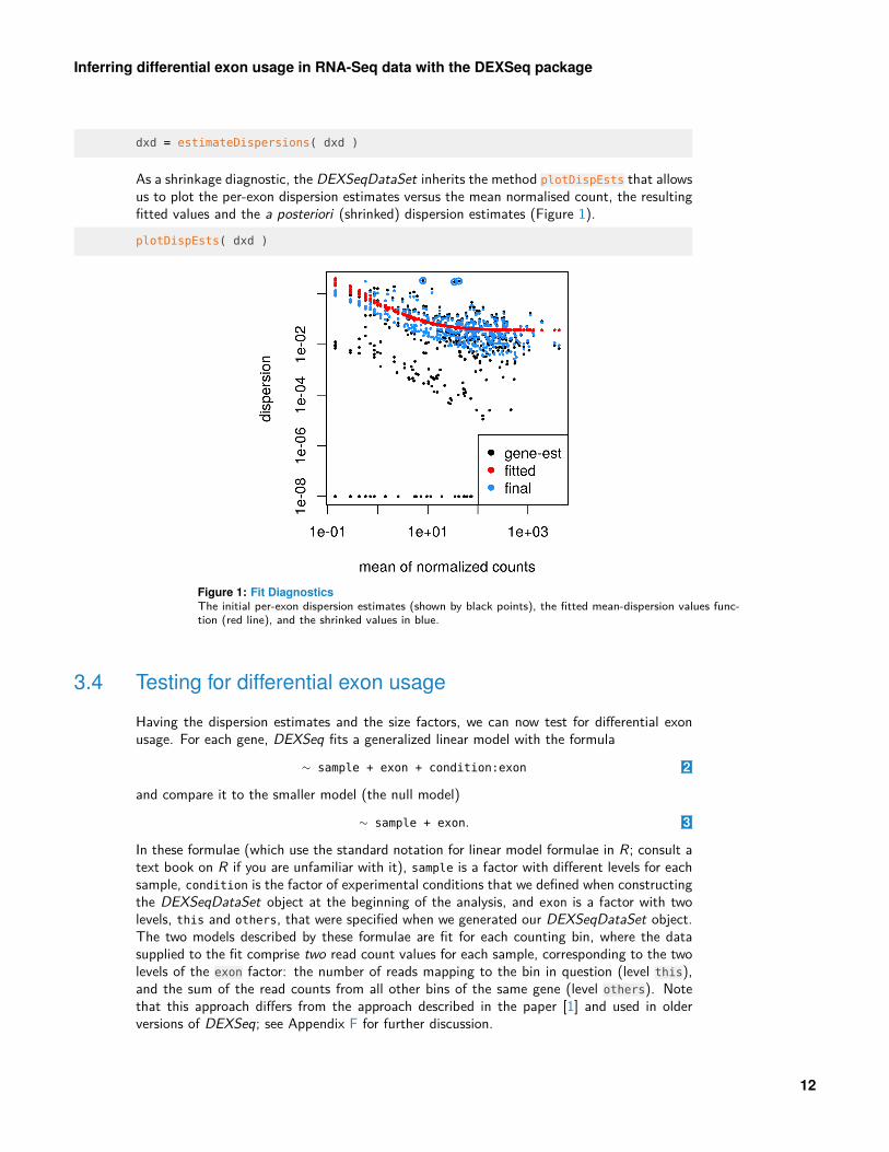
dxd = estimateDispersions( dxd )

As a shrinkage diagnostic, the DEXSeqDataSet inherits the method plotDispEsts that allowsus to plot the per-exon dispersion estimates versus the mean normalised count, the resultingfitted values and the a posteriori (shrinked) dispersion estimates (Figure 1).plotDispEsts( dxd )

Figure 1: Fit DiagnosticsThe initial per-exon dispersion estimates (shown by black points), the fitted mean-dispersion values func-tion (red line), and the shrinked values in blue.

3.4 Testing for differential exon usage

Having the dispersion estimates and the size factors, we can now test for differential exonusage. For each gene, DEXSeq fits a generalized linear model with the formula

∼ sample + exon + condition:exon 2

and compare it to the smaller model (the null model)

∼ sample + exon. 3

In these formulae (which use the standard notation for linear model formulae in R; consult atext book on R if you are unfamiliar with it), sample is a factor with different levels for eachsample, condition is the factor of experimental conditions that we defined when constructingthe DEXSeqDataSet object at the beginning of the analysis, and exon is a factor with twolevels, this and others, that were specified when we generated our DEXSeqDataSet object.The two models described by these formulae are fit for each counting bin, where the datasupplied to the fit comprise two read count values for each sample, corresponding to the twolevels of the exon factor: the number of reads mapping to the bin in question (level this),and the sum of the read counts from all other bins of the same gene (level others). Notethat this approach differs from the approach described in the paper [1] and used in olderversions of DEXSeq; see Appendix F for further discussion.

12


Readers familiar with linear model formulae might find one aspect of Equation 2 surprising:We have an interaction term condition:exon, but denote no main effect for condition.Note, however, that all observations from the same sample are also from the same condition,i.e., the condition main effects are absorbed in the sample main effects, because the sample

factor is nested within the condition factor.The deviances of both fits are compared using a χ2-distribution, providing a p value. Basedon this p-value, we can decide whether the null model 4 is sufficient to explain the data,or whether it may be rejected in favour of the alternative, model 2 , which contains aninteraction coefficient for condition:exon. The latter means that the fraction of the gene’sreads that fall onto the exon under the test differs significantly between the experimentalconditions.The function testForDEU performs these tests for each exon in each gene.dxd = testForDEU( dxd )

The resulting DEXSeqDataSet object contains slots with information regarding the test.For some uses, we may also want to estimate relative exon usage fold changes. To this end,we call estimateExonFoldChanges. Exon usage fold changes are calculated based on thecoefficients of a GLM fit that uses the formula

count ∼ condition + exon + condition:exon, 4

where “condition” can be replaced with any of the column names of colData (see man pagesfor details). The resulting coefficients allow the estimation of changes on the usage of exonsacross different conditions. Note that the differences on exon usage are distinguished fromgene expression differences across conditions. For example, consider the case of a gene thatis differentially expressed between conditions and has one exon that is differentially usedbetween conditions. From the coefficients of the fitted model, it is possible to distinguishoverall gene expression effects, that alter the counts from all the exons, from exon usageeffects, that are captured by the interaction term condition:exon and that affect the eachexon individually.dxd = estimateExonFoldChanges( dxd, fitExpToVar="condition")

So far in the pipeline, the intermediate and final results have been stored in the meta data of aDEXSeqDataSet object, they can be accessed using the function mcol. In order to summarizethe results without showing the values from intermediate steps, we call the function DEXSe

qResults. The result is a DEXSeqResults object, which is a subclass of a DataFrame object.dxr1 = DEXSeqResults( dxd )

dxr1

##

## LRT p-value: full vs reduced

##


## groupID featureID exonBaseMean

## <character> <character> <numeric>

## FBgn0000256:E001 FBgn0000256 E001 58.3431235035746

## FBgn0000256:E002 FBgn0000256 E002 103.332775062259

## FBgn0000256:E003 FBgn0000256 E003 326.47632106146

## FBgn0000256:E004 FBgn0000256 E004 253.65479841846

13


## FBgn0000256:E005 FBgn0000256 E005 60.6376967433858

## ... ... ... ...

## FBgn0261573:E012 FBgn0261573 E012 23.0842247576214

## FBgn0261573:E013 FBgn0261573 E013 9.79723063487541

## FBgn0261573:E014 FBgn0261573 E014 87.4967807998318

## FBgn0261573:E015 FBgn0261573 E015 268.255660671879

## FBgn0261573:E016 FBgn0261573 E016 304.151344294724

## dispersion stat


## FBgn0000256:E001 0.0171917183110422 8.23505533276148e-06

## FBgn0000256:E002 0.00734736583057476 1.57577430142797

## FBgn0000256:E003 0.0104806430182092 0.0357357766681901

## FBgn0000256:E004 0.0110041990870349 0.169540730442577

## FBgn0000256:E005 0.0440296686633544 0.0291053315444856

## ... ... ...

## FBgn0261573:E012 0.0219839757906845 8.40078620496956

## FBgn0261573:E013 0.247551175399698 1.15523263908818

## FBgn0261573:E014 0.0330407155118728 1.11856678841104

## FBgn0261573:E015 0.0120125776234099 2.59830940171975

## FBgn0261573:E016 0.0998525959735577 0.146583499866495

## pvalue padj control

## <numeric> <numeric> <numeric>

## FBgn0000256:E001 0.997710330884085 1 11.0274690368631

## FBgn0000256:E002 0.209370422773832 1 13.2499830375346

## FBgn0000256:E003 0.850062181531059 1 18.9102858849545

## FBgn0000256:E004 0.68052029796093 1 17.702915654299

## FBgn0000256:E005 0.8645360588425 1 10.9937155054498

## ... ... ... ...

## FBgn0261573:E012 0.00375058764137609 0.0977359014782123 6.61691879517948

## FBgn0261573:E013 0.282456447891503 1 5.9708001097303

## FBgn0261573:E014 0.290227270867409 1 13.1912987055365

## FBgn0261573:E015 0.106977775469607 0.965631518582576 18.424533553599

## FBgn0261573:E016 0.701821905229384 1 18.9129561366298

## knockdown log2fold_knockdown_control


## FBgn0000256:E001 10.8820481489974 -0.0513597088461193

## FBgn0000256:E002 13.572177384269 0.103653696151658

## FBgn0000256:E003 18.6029373071523 -0.0895554434858425

## FBgn0000256:E004 17.2692066060147 -0.128321913156379

## FBgn0000256:E005 11.1005587613667 0.037569752559369

## ... ... ...

## FBgn0261573:E012 8.47411808234681 0.832681772274426

## FBgn0261573:E013 3.79997305944298 -1.39556088414956

## FBgn0261573:E014 11.9485055479892 -0.410998955270551

## FBgn0261573:E015 17.2650554422063 -0.34149038224073

## FBgn0261573:E016 18.1441019245549 -0.22459531558904

## genomicData countData

## <GRanges> <matrix>

## FBgn0000256:E001 chr2L:3872658-3872947:- 92:28:43:...

## FBgn0000256:E002 chr2L:3873019-3873322:- 124:80:91:...

## FBgn0000256:E003 chr2L:3873385-3874395:- 340:241:262:...

14


## FBgn0000256:E004 chr2L:3874450-3875302:- 250:189:201:...

## FBgn0000256:E005 chr2L:3878895-3879067:- 96:38:39:...

## ... ... ...

## FBgn0261573:E012 chrX:19421654-19421867:+ 37:23:38:...

## FBgn0261573:E013 chrX:19422668-19422673:+ 8:3:6:...

## FBgn0261573:E014 chrX:19422674-19422856:+ 75:66:92:...

## FBgn0261573:E015 chrX:19422927-19423634:+ 264:234:245:...

## FBgn0261573:E016 chrX:19423707-19424937:+ 611:187:188:...

## transcripts

## <list>






## ... ...

## FBgn0261573:E012 FBtr0302863

## FBgn0261573:E013 c("FBtr0302863", "FBtr0302864")

## FBgn0261573:E014 c("FBtr0302862", "FBtr0302863", "FBtr0302864")



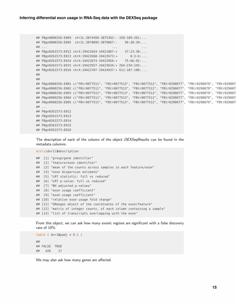
The description of each of the column of the object DEXSeqResults can be found in themetadata columns.mcols(dxr1)$description

## [1] "group/gene identifier"

## [2] "feature/exon identifier"

## [3] "mean of the counts across samples in each feature/exon"

## [4] "exon dispersion estimate"

## [5] "LRT statistic: full vs reduced"

## [6] "LRT p-value: full vs reduced"

## [7] "BH adjusted p-values"

## [8] "exon usage coefficient"

## [9] "exon usage coefficient"

## [10] "relative exon usage fold change"

## [11] "GRanges object of the coordinates of the exon/feature"

## [12] "matrix of integer counts, of each column containing a sample"

## [13] "list of transcripts overlapping with the exon"

From this object, we can ask how many exonic regions are significant with a false discoveryrate of 10%:table ( dxr1$padj < 0.1 )

##

## FALSE TRUE

## 426 17

We may also ask how many genes are affected

15


table ( tapply( dxr1$padj < 0.1, dxr1$groupID, any ) )

##

## FALSE TRUE

## 20 9

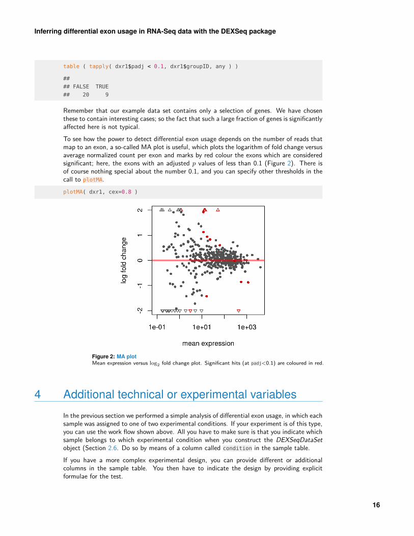
Remember that our example data set contains only a selection of genes. We have chosenthese to contain interesting cases; so the fact that such a large fraction of genes is significantlyaffected here is not typical.To see how the power to detect differential exon usage depends on the number of reads thatmap to an exon, a so-called MA plot is useful, which plots the logarithm of fold change versusaverage normalized count per exon and marks by red colour the exons which are consideredsignificant; here, the exons with an adjusted p values of less than 0.1 (Figure 2). There isof course nothing special about the number 0.1, and you can specify other thresholds in thecall to plotMA.plotMA( dxr1, cex=0.8 )

Figure 2: MA plotMean expression versus log2 fold change plot. Significant hits (at padj<0.1) are coloured in red.

4 Additional technical or experimental variables

In the previous section we performed a simple analysis of differential exon usage, in which eachsample was assigned to one of two experimental conditions. If your experiment is of this type,you can use the work flow shown above. All you have to make sure is that you indicate whichsample belongs to which experimental condition when you construct the DEXSeqDataSetobject (Section 2.6. Do so by means of a column called condition in the sample table.If you have a more complex experimental design, you can provide different or additionalcolumns in the sample table. You then have to indicate the design by providing explicitformulae for the test.

16


In the pasilla dataset, some samples were sequenced in single-end and others in paired-endmode. Possibly, this influenced counts and should hence be accounted for. We therefore usethis as an example for a complex design.When we constructed the DEXSeqDataSet object in Section 2.6, we provided in the sampletable an additional column called libType, which has been stored in the object:sampleAnnotation(dxd)


## sample condition libType sizeFactor

## <factor> <factor> <factor> <numeric>

## 1 treated1 knockdown single-end 1.33594373443595

## 2 treated2 knockdown paired-end 0.799584782672769

## 3 treated3 knockdown paired-end 0.922476585546881

## 4 untreated1 control single-end 0.990898972177499

## 5 untreated2 control single-end 1.56799206105375

## 6 untreated3 control paired-end 0.838396326089713

## 7 untreated4 control paired-end 0.830056383048978

We specify two design formulae, which indicate that the libType factor should be treated asa blocking factor:formulaFullModel = ~ sample + exon + libType:exon + condition:exon

formulaReducedModel = ~ sample + exon + libType:exon

Compare these formulae with the default formulae 2 , 4 given in Section 3.4. We haveadded, in both the full model and the reduced model, the term libType:exon. Therefore,any dependence of exon usage on library type will be absorbed by this term and accountedfor equally in the full and a reduced model, and the likelihood ratio test comparing them willonly detect differences in exon usage that can be attributed to condition, independent oftype.Next, we estimate the dispersions. This time, we need to inform the estimateDispersions

function about our design by providing the full model’s formula, which should be used insteadof the default formula 2 .dxd = estimateDispersions( dxd, formula = formulaFullModel )

The test function now needs to be informed about both formulaedxd = testForDEU( dxd,

reducedModel = formulaReducedModel,

fullModel = formulaFullModel )

Finally, we get a summary table, as before.dxr2 = DEXSeqResults( dxd )

How many significant DEU cases have we got this time?table( dxr2$padj < 0.1 )

##

## FALSE TRUE

## 393 22

17


We can now compare with the previous result:table( before = dxr1$padj < 0.1, now = dxr2$padj < 0.1 )

## now

## before FALSE TRUE

## FALSE 392 6

## TRUE 1 16

Accounting for the library type has allowed us to find six more hits, which confirms thataccounting for the covariate improves power.

5 Visualization

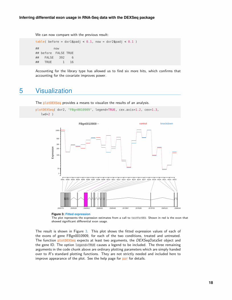
The plotDEXSeq provides a means to visualize the results of an analysis.plotDEXSeq( dxr2, "FBgn0010909", legend=TRUE, cex.axis=1.2, cex=1.3,

lwd=2 )

1

10

100

1000

200

300

500

Exp

ress

ion

E001 E002 E003 E004 E005 E006 E007 E008 E009 E010 E011 E012 E013 E014 E015 E016 E017 E018 E019 E020 E021 E022 E023

2555775 2559193 2562612 2566030 2569448 2572867 2576285 2579703 2583122 2586540

FBgn0010909 − control knockdown

Figure 3: Fitted expressionThe plot represents the expression estimates from a call to testForDEU. Shown in red is the exon thatshowed significant differential exon usage.

The result is shown in Figure 3. This plot shows the fitted expression values of each ofthe exons of gene FBgn0010909, for each of the two conditions, treated and untreated.The function plotDEXSeq expects at least two arguments, the DEXSeqDataSet object andthe gene ID. The option legend=TRUE causes a legend to be included. The three remainingarguments in the code chunk above are ordinary plotting parameters which are simply handedover to R’s standard plotting functions. They are not strictly needed and included here toimprove appearance of the plot. See the help page for par for details.

18


Optionally, one can also visualize the transcript models (Figure 4), which can be useful forputting differential exon usage results into the context of isoform regulation.plotDEXSeq( dxr2, "FBgn0010909", displayTranscripts=TRUE, legend=TRUE,

cex.axis=1.2, cex=1.3, lwd=2 )

1

10

100

1000

200

300

500

Exp

ress

ion


2555775 2559193 2562612 2566030 2569448 2572867 2576285 2579703 2583122 2586540


Figure 4: TranscriptsAs in Figure 3, but including the annotated transcript models.

Other useful options are to look at the count values from the individual samples, rather thanat the model effect estimates. For this display (option norCounts=TRUE), the counts arenormalized by dividing them by the size factors (Figure 5).plotDEXSeq( dxr2, "FBgn0010909", expression=FALSE, norCounts=TRUE,

legend=TRUE, cex.axis=1.2, cex=1.3, lwd=2 )

As explained in Section 1, DEXSeq is designed to find changes in relative exon usage, i. e.,changes in the expression of individual exons that are not simply the consequence of overallup- or down-regulation of the gene. To visualize such changes, it is sometimes advantageousto remove overall changes in expression from the plots. Use the (somewhat misnamed) optionsplicing=TRUE for this purpose.plotDEXSeq( dxr2, "FBgn0010909", expression=FALSE, splicing=TRUE,

legend=TRUE, cex.axis=1.2, cex=1.3, lwd=2 )

To generate an easily browsable, detailed overview over all analysis results, the package pro-vides an HTML report generator, implemented in the function DEXSeqHTML. This functionuses the package hwriter [10] to create a result table with links to plots for the significantresults, allowing a more detailed exploration of the results.DEXSeqHTML( dxr2, FDR=0.1, color=c("#FF000080", "#0000FF80") )

19


10

100

1000

200

300

500N

orm

aliz

ed c

ount

s


2555775 2559193 2562612 2566030 2569448 2572867 2576285 2579703 2583122 2586540


Figure 5: Normalized countsAs in Figure 3, with normalized count values of each exon in each of the samples.

1

10

100

1000

200

300

500

Exo

n us

age


2555775 2559193 2562612 2566030 2569448 2572867 2576285 2579703 2583122 2586540


Figure 6: Fitted splicingThe plot represents the estimated effects, as in Figure 3, but after subtraction of overall changes in geneexpression.

20


6 Parallelization and large number of samples

DEXSeq analyses can be computationally heavy, especially with data sets that comprise alarge number of samples, or with genomes containing genes with large numbers of exons.While some steps of the analysis work on the whole data set, the computational load canbe parallelized for some steps. We use the package BiocParallel, and implemented the BP

PARAM parameter of the functions estimateDispersions, testForDEU and estimateExonFold

Changes:BPPARAM = MultiCoreParam(workers=4)

dxd = estimateSizeFactors( dxd )

dxd = estimateDispersions( dxd, BPPARAM=BPPARAM)

dxd = testForDEU( dxd, BPPARAM=BPPARAM)

dxd = estimateExonFoldChanges(dxd, BPPARAM=BPPARAM)

For running analysis with a large number of samples (e.g. more than 100), we recommendconfiguring BatchJobsParam classes to BPPARAM in order to distribute the calculationsacross a computer cluster and significantly reduce running times. Users might also considerreducing the number of tests by filtering for lowly expressed isoforms or exonic regions withlow counts. Appart from reducing running times, this filtering step also leads to more accurateresults [11].

7 Perform a standard differential exon usage analy-sis in one command

In the previous sections, we went through the analysis step by step. Once you are sufficientlyconfident about the work flow for your data, its invocation can be streamlined by the wrapperfunction DEXseq, which runs the analysis shown above through a single function call.In the simplest case, construct the DEXSeqDataSet as shown in Section 2 or in Appendix B,then run DEXSeq passing the DEXSeqDataSet as only argument, this function will output aDEXSeqResults object.dxr = DEXSeq(dxd)

class(dxr)

## [1] "DEXSeqResults"

## attr(,"package")

## [1] "DEXSeq"

21


APPENDIX

A Controlling FDR at the gene level

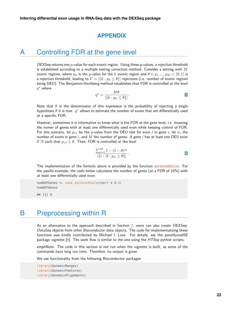
DEXSeq returns one p-value for each exonic region. Using these p-values, a rejection thresholdis established according to a multiple testing correction method. Consider a setting with Mexonic regions, where pk is the p-value for the k exonic region and θ ∈ p1, ..., pM ⊂ [0, 1] isa rejection threshold, leading to V = |{k : pk ≤ θ}| rejections (i.e. number of exonic regionsbeing DEU). The Benjamini-Hochberg method establishes that FDR is controlled at the levelq∗ where

q∗ =Mθ

|{k : pk ≤ θ}|. 5

Note that θ in the denominator of this expression is the probability of rejecting a singlehypothesis if it is true. q∗ allows to estimate the number of exons that are differentially usedat a specific FDR.However, sometimes it is informative to know what is the FDR at the gene level, i.e. knowingthe numer of genes with at least one differentially used exon while keeping control of FDR.For this scenario, let pi,l be the p-value from the DEU test for exon l in gene i, let ni thenumber of exons in gene i, and M the number of genes. A gene i has at least one DEU exonif ∃l such that pi,l ≤ θ. Then, FDR is controlled at the level∑M

i=1 1− (1− θ)ni

|{i : ∃l : pil ≤ θ}|. 6

The implementation of the formula above is provided by the function perGeneQValue. Forthe pasilla example, the code below calculates the number of genes (at a FDR of 10%) withat least one differentially used exon.numbOfGenes <- sum( perGeneQValue(dxr) < 0.1)

numbOfGenes

## [1] 9

B Preprocessing within R

As an alternative to the approach described in Section 2, users can also create DEXSeq-DataSeq objects from other Bioconductor data objects. The code for implementationg thesefunctions was kindly contributed by Michael I. Love. For details, see the parathyroidSEpackage vignette [8]. The work flow is similar to the one using the HTSeq python scripts.emphNote: The code in this section is not run when the vignette is built, as some of thecommands have long run time. Therefore, no output is given.We use functionality from the following Bioconductor packageslibrary(GenomicRanges)

library(GenomicFeatures)

library(GenomicAlignments)

22


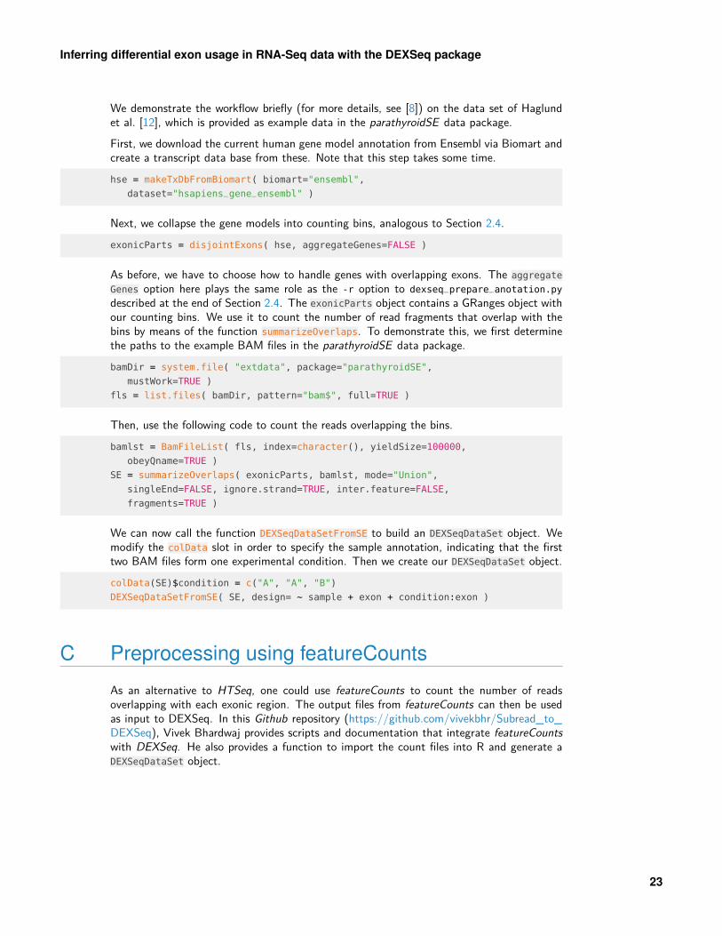
We demonstrate the workflow briefly (for more details, see [8]) on the data set of Haglundet al. [12], which is provided as example data in the parathyroidSE data package.First, we download the current human gene model annotation from Ensembl via Biomart andcreate a transcript data base from these. Note that this step takes some time.hse = makeTxDbFromBiomart( biomart="ensembl",

dataset="hsapiens_gene_ensembl" )

Next, we collapse the gene models into counting bins, analogous to Section 2.4.exonicParts = disjointExons( hse, aggregateGenes=FALSE )

As before, we have to choose how to handle genes with overlapping exons. The aggregate

Genes option here plays the same role as the -r option to dexseq_prepare_anotation.py

described at the end of Section 2.4. The exonicParts object contains a GRanges object withour counting bins. We use it to count the number of read fragments that overlap with thebins by means of the function summarizeOverlaps. To demonstrate this, we first determinethe paths to the example BAM files in the parathyroidSE data package.bamDir = system.file( "extdata", package="parathyroidSE",

mustWork=TRUE )

fls = list.files( bamDir, pattern="bam$", full=TRUE )

Then, use the following code to count the reads overlapping the bins.bamlst = BamFileList( fls, index=character(), yieldSize=100000,

obeyQname=TRUE )

SE = summarizeOverlaps( exonicParts, bamlst, mode="Union",

singleEnd=FALSE, ignore.strand=TRUE, inter.feature=FALSE,

fragments=TRUE )

We can now call the function DEXSeqDataSetFromSE to build an DEXSeqDataSet object. Wemodify the colData slot in order to specify the sample annotation, indicating that the firsttwo BAM files form one experimental condition. Then we create our DEXSeqDataSet object.colData(SE)$condition = c("A", "A", "B")

DEXSeqDataSetFromSE( SE, design= ~ sample + exon + condition:exon )

C Preprocessing using featureCounts

As an alternative to HTSeq, one could use featureCounts to count the number of readsoverlapping with each exonic region. The output files from featureCounts can then be usedas input to DEXSeq. In this Github repository (https://github.com/vivekbhr/Subread_to_DEXSeq), Vivek Bhardwaj provides scripts and documentation that integrate featureCountswith DEXSeq. He also provides a function to import the count files into R and generate aDEXSeqDataSet object.

23

https://github.com/vivekbhr/Subread_to_DEXSeq

https://github.com/vivekbhr/Subread_to_DEXSeq


D Further accessors

The function geneIDs returns the gene ID column of the feature data as a character vector,and the function exonIDs return the exon ID column as a factor.head( geneIDs(dxd) )

## [1] "FBgn0000256" "FBgn0000256" "FBgn0000256" "FBgn0000256" "FBgn0000256"

## [6] "FBgn0000256"

head( exonIDs(dxd) )

## [1] "E001" "E002" "E003" "E004" "E005" "E006"

These functions are useful for subsetting an DEXSeqDataSet object.

E Overlap operations

The methods subsetByOverlaps and findOverlaps have been implemented for the DEXSe-qResults object, the query argument must be a DEXSeqResults object.interestingRegion = GRanges( "chr2L",

IRanges(start=3872658, end=3875302) )

subsetByOverlaps( x=dxr, ranges=interestingRegion )

##

## LRT p-value: full vs reduced

##


## groupID featureID exonBaseMean

## <character> <character> <numeric>

## FBgn0000256:E001 FBgn0000256 E001 58.3431235035746

## FBgn0000256:E002 FBgn0000256 E002 103.332775062259

## FBgn0000256:E003 FBgn0000256 E003 326.47632106146

## FBgn0000256:E004 FBgn0000256 E004 253.65479841846

## dispersion stat pvalue


## FBgn0000256:E001 0.0171917183110422 8.23505533276148e-06 0.997710330884085

## FBgn0000256:E002 0.00734736583057476 1.57577430142797 0.209370422773832

## FBgn0000256:E003 0.0104806430182092 0.0357357766681901 0.850062181531059

## FBgn0000256:E004 0.0110041990870349 0.169540730442577 0.68052029796093

## padj control knockdown


## FBgn0000256:E001 1 11.0274690368631 10.8820481489974

## FBgn0000256:E002 1 13.2499830375346 13.572177384269

## FBgn0000256:E003 1 18.9102858849545 18.6029373071523

## FBgn0000256:E004 1 17.702915654299 17.2692066060147

## log2fold_knockdown_control control.1


## FBgn0000256:E001 -0.0513597088461193 11.0274690368631

## FBgn0000256:E002 0.103653696151658 13.2499830375346

24


## FBgn0000256:E003 -0.0895554434858425 18.9102858849545

## FBgn0000256:E004 -0.128321913156379 17.702915654299

## knockdown.1 log2fold_knockdown_control.1


## FBgn0000256:E001 10.8820481489974 -0.0513597088461193

## FBgn0000256:E002 13.572177384269 0.103653696151658

## FBgn0000256:E003 18.6029373071523 -0.0895554434858425

## FBgn0000256:E004 17.2692066060147 -0.128321913156379

## genomicData countData

## <GRanges> <matrix>

## FBgn0000256:E001 chr2L:3872658-3872947:- 92:28:43:...

## FBgn0000256:E002 chr2L:3873019-3873322:- 124:80:91:...

## FBgn0000256:E003 chr2L:3873385-3874395:- 340:241:262:...

## FBgn0000256:E004 chr2L:3874450-3875302:- 250:189:201:...

## transcripts

## <list>





findOverlaps( query=dxr, subject=interestingRegion )

## Hits object with 4 hits and 0 metadata columns:

## queryHits subjectHits

## <integer> <integer>

## [1] 1 1

## [2] 2 1

## [3] 3 1

## [4] 4 1

## -------

## queryLength: 498 / subjectLength: 1

This functions could be useful for further downstream analysis.

F Methodological changes since publication of thepaper

In our paper [1], we suggested to fit for each exon a model that includes separately thecounts for all the gene’s exons. However, this turned out to be computationally inefficientfor genes with many exons, because the many exons required large model matrices, whichare computationally expensive to deal with. We have therefore modified the approach: whenfitting a model for an exon, we now sum up the counts from all the other exon and use onlythe total, rather than the individual counts in the model. Now, computation time per exon isindependent of the number of other exons in the gene, which improved DEXSeq’s scalability.While the p values returned by the two approaches are not exactly equal, the differences werevery minor in the tests that we performed.

25


Deviating from the paper’s notation, we now use the index i to indicate a specific countingbin, with i running through all counting bins of all genes. The samples are indexed with j,as in the paper. We write Kij0 for the count or reads mapped to counting bin i in samplej and Kij1 for the sum of the read counts from all other counting bins in the same gene.Hence, when we write Kijl, the third index l indicates whether we mean the read count forbin i (l = 0) or the sum of counts for all other bins of the same gene (l = 1). As before, wefit a GLM of the negative binomial (NB) family

Kijl ∼ NB(mean = sjµijl, dispersion = αi), 7

now with the model specified in Equation 2 , which we write out as

log2 µijl = βSij + lβEi + βECiρj . 8

This model is fit separately for each counting bin i. The coefficient βSij accounts for thesample-specific contribution (factor sample in Equation 2 ), the term βEi is only includedif l = 1 and hence estimates the logarithm of the ratio Kij1/Kij0 between the counts forall other exons and the counts for the tested exon. As this coefficient is estimated fromdata from all samples, it can be considered as a measure of “average exon usage”. In theR model formula, it is represented by the term exon with its two levels this (l = 0) andothers (l = 1). Finally, the last term, βECi,ρj , captures the interaction condition:exon, i.e.,the change in exon usage if sample j is from experimental condition group ρ(j). Here, thefirst condition, ρ = 0, is absorbed in the sample coefficients, i.e., βECi0 is fixed to zero anddoes not appear in the model matrix.For the dispersion estimation, one dispersion value αi is estimated with Cox-Reid-adjustedmaximum likelihood using the full model given above. A mean-variance relation is fittedusing the individual dispersion values. Finally, the individual values are shrinked towards thefitted values. For more details about this shrinkage approach look at the DESeq2 vignetteand/or its manuscript [9]. For the likelihood ratio test, this full model is fit and comparedwith the fit of the reduced model, which lacks the interaction term βECiρj . As described inSection 4, alternative model formulae can be specified.

G Requirements on GTF files

In the initial preprocessing step described in Section 2.4, the Python script dexseq_prepare_annotation.py is used to convert a GTF file with gene models into a GFF file with collapsedgene models. We recommend to use GTF files downloaded from Ensembl as input for thisscript, as files from other sources may deviate from the format expected by the script. Hence,if you need to use a GTF or GFF file from another source, you may need to convert it to theexpected format. To help with this task, we here give details on how the dexseq_prepare_

annotation.py script interprets a GFF file.• The script only looks at exon lines, i.e., at lines which contain the term exon in the

third (“type”) column. All other lines are ignored.• Of the data in these lines, the information about chromosome, start, end, and strand

(1st, 4th, 5th, and 7th column) are used, and, from the last column, the attributesgene_id and transcript_id. The rest is ignored.

26


• The gene_id attribute is used to see which exons belong to the same gene. It must becalled gene_id (and not Parent as in GFF3 files, or GeneID as in some older GFF files),and it must give the same identifier to all exons from the same gene, even if they arefrom different transcripts of this gene. (This last requirement is not met by GTF filesgenerated by the Table Browser function of the UCSC Genome Browser.)

• The transcript_id attribute is used to build the transcripts attribute in the flattenedGFF file, which indicates which transcripts contain the described counting bin. Thisinformation is needed only to draw the transcript model at the bottom of the plotswhen the displayTranscript option to plotDEXSeq is used.

Therefore, converting a GFF file to make it suitable as input to dexseq_prepare_annotation.

py amounts to making sure that the exon lines have type exon and that the atributes givinggene ID (or gene symbol) and transcript ID are called gene_id and transcript_id, with thisexact spelling. Remember to also take care that the chromosome names match those inyour SAM files, and that the coordinates refer to the reference assembly that you used whenaligning your reads.

H Session Information

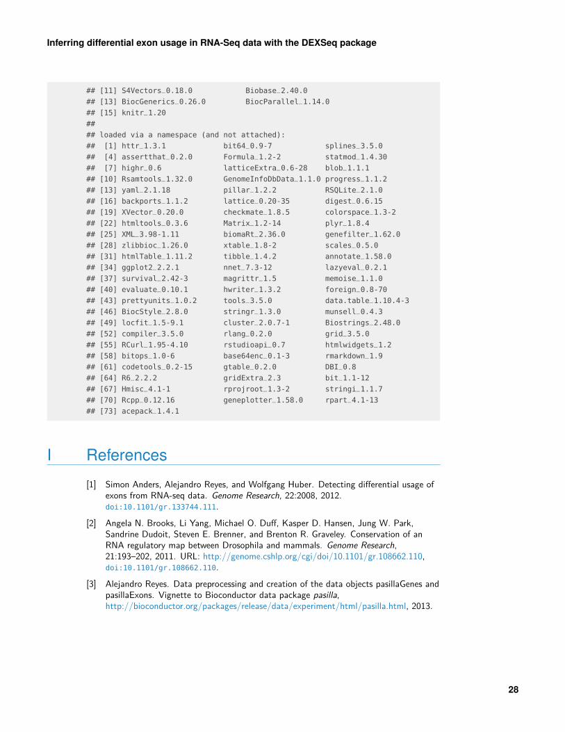
The session information records the versions of all the packages used in the generation of thepresent document.sessionInfo()

## R version 3.5.0 (2018-04-23)

## Platform: x86_64-pc-linux-gnu (64-bit)

## Running under: Ubuntu 16.04.4 LTS

##

## Matrix products: default

## BLAS: /home/biocbuild/bbs-3.7-bioc/R/lib/libRblas.so

## LAPACK: /home/biocbuild/bbs-3.7-bioc/R/lib/libRlapack.so

##

## locale:

## [1] LC_CTYPE=en_US.UTF-8 LC_NUMERIC=C

## [3] LC_TIME=en_US.UTF-8 LC_COLLATE=C

## [5] LC_MONETARY=en_US.UTF-8 LC_MESSAGES=en_US.UTF-8

## [7] LC_PAPER=en_US.UTF-8 LC_NAME=C

## [9] LC_ADDRESS=C LC_TELEPHONE=C

## [11] LC_MEASUREMENT=en_US.UTF-8 LC_IDENTIFICATION=C

##

## attached base packages:

## [1] stats4 parallel stats graphics grDevices utils datasets

## [8] methods base

##

## other attached packages:

## [1] DEXSeq_1.26.0 RColorBrewer_1.1-2

## [3] AnnotationDbi_1.42.0 DESeq2_1.20.0

## [5] SummarizedExperiment_1.10.0 DelayedArray_0.6.0

## [7] matrixStats_0.53.1 GenomicRanges_1.32.0

## [9] GenomeInfoDb_1.16.0 IRanges_2.14.0

27


## [11] S4Vectors_0.18.0 Biobase_2.40.0

## [13] BiocGenerics_0.26.0 BiocParallel_1.14.0

## [15] knitr_1.20

##

## loaded via a namespace (and not attached):

## [1] httr_1.3.1 bit64_0.9-7 splines_3.5.0

## [4] assertthat_0.2.0 Formula_1.2-2 statmod_1.4.30

## [7] highr_0.6 latticeExtra_0.6-28 blob_1.1.1

## [10] Rsamtools_1.32.0 GenomeInfoDbData_1.1.0 progress_1.1.2

## [13] yaml_2.1.18 pillar_1.2.2 RSQLite_2.1.0

## [16] backports_1.1.2 lattice_0.20-35 digest_0.6.15

## [19] XVector_0.20.0 checkmate_1.8.5 colorspace_1.3-2

## [22] htmltools_0.3.6 Matrix_1.2-14 plyr_1.8.4

## [25] XML_3.98-1.11 biomaRt_2.36.0 genefilter_1.62.0

## [28] zlibbioc_1.26.0 xtable_1.8-2 scales_0.5.0

## [31] htmlTable_1.11.2 tibble_1.4.2 annotate_1.58.0

## [34] ggplot2_2.2.1 nnet_7.3-12 lazyeval_0.2.1

## [37] survival_2.42-3 magrittr_1.5 memoise_1.1.0

## [40] evaluate_0.10.1 hwriter_1.3.2 foreign_0.8-70

## [43] prettyunits_1.0.2 tools_3.5.0 data.table_1.10.4-3

## [46] BiocStyle_2.8.0 stringr_1.3.0 munsell_0.4.3

## [49] locfit_1.5-9.1 cluster_2.0.7-1 Biostrings_2.48.0

## [52] compiler_3.5.0 rlang_0.2.0 grid_3.5.0

## [55] RCurl_1.95-4.10 rstudioapi_0.7 htmlwidgets_1.2

## [58] bitops_1.0-6 base64enc_0.1-3 rmarkdown_1.9

## [61] codetools_0.2-15 gtable_0.2.0 DBI_0.8

## [64] R6_2.2.2 gridExtra_2.3 bit_1.1-12

## [67] Hmisc_4.1-1 rprojroot_1.3-2 stringi_1.1.7

## [70] Rcpp_0.12.16 geneplotter_1.58.0 rpart_4.1-13

## [73] acepack_1.4.1

I References

[1] Simon Anders, Alejandro Reyes, and Wolfgang Huber. Detecting differential usage ofexons from RNA-seq data. Genome Research, 22:2008, 2012.doi:10.1101/gr.133744.111.

[2] Angela N. Brooks, Li Yang, Michael O. Duff, Kasper D. Hansen, Jung W. Park,Sandrine Dudoit, Steven E. Brenner, and Brenton R. Graveley. Conservation of anRNA regulatory map between Drosophila and mammals. Genome Research,21:193–202, 2011. URL: http://genome.cshlp.org/cgi/doi/10.1101/gr.108662.110,doi:10.1101/gr.108662.110.

[3] Alejandro Reyes. Data preprocessing and creation of the data objects pasillaGenes andpasillaExons. Vignette to Bioconductor data package pasilla,http://bioconductor.org/packages/release/data/experiment/html/pasilla.html, 2013.

28

http://dx.doi.org/10.1101/gr.133744.111

http://genome.cshlp.org/cgi/doi/10.1101/gr.108662.110

http://dx.doi.org/10.1101/gr.108662.110

http://bioconductor.org/packages/release/data/experiment/html/pasilla.html


[4] Daehwan Kim, Geo Pertea, Cole Trapnell, Harold Pimentel, Ryan Kelley, and StevenSalzberg. Tophat2: accurate alignment of transcriptomes in the presence of insertions,deletions and gene fusions. Genome Biology, 14(4):R36, 2013. URL:http://genomebiology.com/2013/14/4/R36, doi:10.1186/gb-2013-14-4-r36.

[5] Thomas D. Wu and Serban Nacu. Fast and SNP-tolerant detection of complexvariants and splicing in short reads. Bioinformatics, 26(7):873–881, 2010. URL:http://bioinformatics.oxfordjournals.org/content/26/7/873.abstract, arXiv:http://bioinformatics.oxfordjournals.org/content/26/7/873.full.pdf+html,doi:10.1093/bioinformatics/btq057.

[6] Alexander Dobin, Carrie A. Davis, Felix Schlesinger, Jorg Drenkow, Chris Zaleski,Sonali Jha, Philippe Batut, Mark Chaisson, and Thomas R. Gingeras. STAR: ultrafastuniversal RNA-seq aligner. Bioinformatics, 29(1):15–21, 2013. URL:http://bioinformatics.oxfordjournals.org/content/29/1/15.abstract, arXiv:http://bioinformatics.oxfordjournals.org/content/29/1/15.full.pdf+html,doi:10.1093/bioinformatics/bts635.

[7] Simon Anders, Davis J. McCarthy, Yunshen Chen, Michal Okoniewski, Gordon K.Smyth, Wolfgang Huber, and Mark D. Robinson. Count-based differential expressionanalysis of RNA sequencing data using R and Bioconductor. Nature Protocols, 8:1765,2013. doi:10.1038/nprot.2013.099.

[8] Michael Love. SummarizedExperiment for RNA-Seq of primary cultures of parathyroidtumors by Haglund et al., J Clin Endocrinol Metab 2012. Vignette to Bioconductordata package parathyroidSE,http://bioconductor.org/packages/release/data/experiment/html/parathyroidSE.html,2013.

[9] Michael I Love, Wolfgang Huber, and Simon Anders. Moderated estimation of foldchange and dispersion for RNA-Seq data with DESeq2. bioRxiv, 2014. URL:http://biorxiv.org/content/early/2014/02/19/002832,arXiv:http://biorxiv.org/content/early/2014/02/19/002832.full.pdf,doi:10.1101/002832.

[10] Gregoire Pau and Wolfgang Huber. The hwriter package. The R Journal, 1:22, 2009.URL: http://journal.r-project.org/archive/2009-1/RJournal_2009-1_Pau+Huber.pdf.

[11] Charlotte Soneson, Katarina L. Matthes, Malgorzata Nowicka, Charity W. Law, andMark D. Robinson. Isoform prefiltering improves performance of count-based methodsfor analysis of differential transcript usage. Genome Biology, 17(1):1–15, 2016. URL:http://dx.doi.org/10.1186/s13059-015-0862-3, doi:10.1186/s13059-015-0862-3.

[12] Felix Haglund, Ran Ma, Mikael Huss, Luqman Sulaiman, Ming Lu, Inga-Lena Nilsson,Anders Höög, C. Christofer Juhlin, Johan Hartman, and Catharina Larsson. Evidenceof a functional estrogen receptor in parathyroid adenomas. Journal of ClinicalEndocrinology & Metabolism, 97(12), 2012. URL:http://jcem.endojournals.org/content/97/12/4631.abstract,arXiv:http://jcem.endojournals.org/content/97/12/4631.full.pdf+html,doi:10.1210/jc.2012-2484.

29

http://genomebiology.com/2013/14/4/R36

http://dx.doi.org/10.1186/gb-2013-14-4-r36

http://bioinformatics.oxfordjournals.org/content/26/7/873.abstract

http://arxiv.org/abs/http://bioinformatics.oxfordjournals.org/content/26/7/873.full.pdf+html


http://dx.doi.org/10.1093/bioinformatics/btq057

http://bioinformatics.oxfordjournals.org/content/29/1/15.abstract



http://dx.doi.org/10.1093/bioinformatics/bts635

http://dx.doi.org/10.1038/nprot.2013.099

http://bioconductor.org/packages/release/data/experiment/html/parathyroidSE.html

http://biorxiv.org/content/early/2014/02/19/002832

http://arxiv.org/abs/http://biorxiv.org/content/early/2014/02/19/002832.full.pdf

http://dx.doi.org/10.1101/002832

http://journal.r-project.org/archive/2009-1/RJournal_2009-1_Pau+Huber.pdf

http://dx.doi.org/10.1186/s13059-015-0862-3

http://dx.doi.org/10.1186/s13059-015-0862-3

http://jcem.endojournals.org/content/97/12/4631.abstract

http://arxiv.org/abs/http://jcem.endojournals.org/content/97/12/4631.full.pdf+html

http://dx.doi.org/10.1210/jc.2012-2484

InferringdifferentialexonusageinRNA-Seq data with the ... ·...

Documents

Transcript of InferringdifferentialexonusageinRNA-Seq data with the ... ·...