Inferring Tracklets for Multi-Object Tracking

Jan Prokaj1, Mark Duchaineau2, and Gerard Medioni1

1University of Southern California , Los Angeles, CA 90089 , {prokaj|medioni}@usc.edu2Lawrence Livermore National Laboratory , Livermore, CA 94550, duchaineau@llnl.gov

Abstract

Recent work on multi-object tracking has shown thepromise of tracklet-based methods. In this work we presenta method which infers tracklets then groups them intotracks. It overcomes some of the disadvantages of exist-ing methods, such as the use of heuristics or non-realisticconstraints. The main idea is to formulate the data associ-ation problem as inference in a set of Bayesian networks.This avoids exhaustive evaluation of data association hy-potheses, provides a confidence estimate of the solution,and handles split-merge observations. Consistency of mo-tion and appearance is the driving force behind finding theMAP data association estimate.

The computed tracklets are then used in a completemulti-object tracking algorithm, which is evaluated on a ve-hicle tracking task in an aerial surveillance context. Verygood performance is achieved on challenging video se-quences. Track fragmentation is nearly non-existent, andfalse alarm rates are low.

1. Introduction

Object tracking is a well studied problem that has re-ceived considerable attention in the computer vision com-munity, and does not need much of an introduction. Solv-ing this problem will immediately benefit many applica-tions, such as surveillance and human computer interaction,and provide necessary information with high confidence forhigher-level reasoning tasks, such as activity or event recog-nition, and behavior analysis. Many approaches have beenproposed [17], each having advantages in a particular con-text. Here we focus on multi-object tracking, where the goalis to determine a spatio-temporal description of the movingobjects in the scene.

Tracking of multiple objects naturally has to deal withthe same issues encountered in classic tracking, such as oc-clusion, and changes in illumination and appearance. It

also brings additional challenges, namely associating theevidence in the video with an unknown number of ob-jects, and object-object interaction, which results in a many-many mapping between observations (detections or mea-surements) and objects in every frame. In other words,one observation may be associated with multiple objects,or multiple observations may be associated with one objectdue to occlusion or noise. This presents a large data as-sociation problem, which is expensive to solve optimally:a correct data association requires looking ahead in time,but this in turn causes an exponential growth of the searchspace.

Currently the most successful algorithms for multi-object tracking solve the data association problem hierar-chically [13, 2, 6, 8]. They first determine short tracks, ortracklets, and then link these tracklets into longer tracks inone or more steps. Tracklets are usually determined by us-ing a nearest neighbor association [13], some affinity mea-sure [6], or particle filtering [8]. However, each of thesehas some disadvantages. Nearest neighbor association is aheuristic that is likely to make incorrect associations whenobjects are close together. Affinity measures, while con-servative, assume a non-overlap constraint. Particle filter-ing works better, but with a lot of objects or noise in thescene, and longer time intervals, the number of hypothe-ses significantly increases, and the computational cost be-comes prohibitive. An alternative solution is proposed in[15] where the scene is first divided into grid cells and theHungarian algorithm is then used to estimate the associationof detections from one frame to the next. One disadvantagehere is that weights in the bipartite graph matching problemare based on local context that is assumed to stay constant,which may not work as well in urban areas where vehiclesmake turns.

The primary contribution of this work is an algorithmfor inferring tracklets, which does not require an exhaus-tive evaluation of data association hypotheses, is a MAPestimate, rather than a heuristic, does not assume one-onemapping between observations and objects, and provides

a confidence measure on each tracklet. The algorithm ac-complishes this by formulating the problem as inference ina set of Bayesian networks, and uses consistency of motionand appearance as the driving force. The computed track-lets are then used in a complete multi-object tracking algo-rithm, which is evaluated on a vehicle tracking task in anaerial surveillance context.

2. Related WorkThe classic algorithms for multi-object tracking are Joint

Probabilistic Data Association filter (JDPAF) [4], and Mul-tiple Hypothesis Tracking (MHT) [14, 3]. Both of thesemethods operate on a set of data association hypotheses.JPDAF uses all hypotheses, weighted according to the pos-terior, in determining the next state, while MHT keeps thecandidate hypotheses in memory and does not make a de-cision until any ambiguities are resolved. In addition to re-quiring exponential space and time, a significant weaknessof these algorithms is that they assume one-one mappingbetween observations and objects.

More useful approaches that handle occlusions in multi-object tracking are [19] and [7]. In [19], a globally optimaldata association was achieved by encoding the data associ-ation problem in a network flow graph, and solving with aminimum cut. While this strategy is compelling, the methodassumes that two tracks cannot have overlapping observa-tions, which happens with merged observations. A linearprogramming formulation, which allows for occlusions, butassumes spatial layout constraints, was presented in [7].

There have been several attempts to handle multiplesplit-merge events in observations. A particle filtering ap-proach was presented in [9]. There, a more efficient solutionis obtained by assuming Gaussian motion, and computingthe target state analytically for each sampled data associa-tion. A particle filtering approach using Adaboost for morerobust detections is presented in [12]. Another sampling al-gorithm, using data-driven MCMC, was introduced in [18].Spatio-temporal smoothness in motion and appearance waskey to recovering the tracks of an unknown number of tar-gets.

Perera et al. described an algorithm for multi-objecttracking that handles long occlusions, and split-merge con-ditions in [13]. They begin with detecting a set of tracklets,and subsequently link these tracklets into long tracks. Link-ing is accomplished with the Hungarian algorithm and usingan approximation that does not require an exhaustive searchof associations. This algorithm requires that the initial setof tracklets be reliable. More tracklet-based approaches tomulti-object tracking followed in [6, 8]. An affinity mea-sure to determine tracklets was used in [6], and a particlefilter in [8].

It is clear that tracklet-based approaches have merit, butas mentioned earlier, the current algorithms to determine

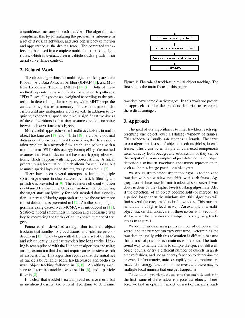
Figure 1: The role of tracklets in multi-object tracking. Thefirst step is the main focus of this paper.

tracklets have some disadvantages. In this work we presentan approach to infer the tracklets that tries to overcomethese disadvantages.

3. Approach

The goal of our algorithm is to infer tracklets, each rep-resenting one object, over a (sliding) window of frames.This window is usually 4-8 seconds in length. The inputto our algorithm is a set of object detections (blobs) in eachframe. These can be as simple as connected componentstaken directly from background subtraction, or they can bethe output of a more complex object detector. Each objectdetection also has an associated appearance representation,such as the raw image patch, or a histogram.

We would like to emphasize that our goal is to find validtracklets within a window that shifts with each frame. Ag-gregation of these tracklets into tracks that span several win-dows is done by the (higher-level) tracking algorithm. Alsoif the detections of an object become split (or merged) fora period longer than the window size, this algorithm willfind several (or one) tracklets in the window. This must behandled at the higher-level as well. An example of a multi-object tracker that takes care of these issues is in Section 4.A flow-chart that clarifies multi-object tracking using track-lets is in Figure 1.

We do not assume an a priori number of objects in thescene, and the number can vary over time. Determining thetracklets optimally with this relaxation is difficult, becausethe number of possible associations is unknown. The tradi-tional way to handle this is to sample the space of differentobject counts, or try a different number of objects in an it-erative fashion, and use an energy function to determine theanswer. Unfortunately, unless simplifying assumptions aremade, this energy function is nonconvex, and there may bemultiple local minima that one get trapped in.

To avoid this problem, we assume that each detection inthe first frame of the window is a potential object. There-fore, we find an optimal tracklet, or a set of tracklets, start-

ing at each detection in the first window frame. This is nota problem, because for detections that are false alarms, themodel of a valid tracklet (consistency of motion and appear-ance) is not satisfied, and the tracklet is discarded. Track-lets that start in the second or later frame of the window arefound when the sliding window shifts to that frame.

3.1. Problem formulation

If the initial detection of an object is given to us, weknow there must be another detected instance of that objectlocated “nearby” in subsequent frames. We are assumingthere are no missed detections (due to occlusion or else) fornow, but split detections, or split-merge detections, do notpose a problem, and this statement still holds. Therefore,the optimal tracklet, or a set of tracklets, that we want tofind must be composed of a series of “nearby” detections.This can be expressed in a detection tree. For a window sizeof T frames, this tree would have T levels. A node in levelt has links to those nodes in level t+1, which are “nearby.”The root of the tree, t = 0, represents the initial detection.The definition of nearby can vary with dataset, but, for ex-ample, in aerial surveillance of urban areas, this value canbe set according to the maximum expected velocity of vehi-cles, and video resolution.

The number of possible tracklets and tracklet combina-tions arising from this detection tree is huge, and we cer-tainly do not want to evaluate every hypothesis. Instead,we realize that every such hypothesis is making a decisionabout including or not including each detection. In otherwords, this is just a binary labeling, or segmentation prob-lem. The valid detections need to be separated from theinvalid detections. The invalid detections are detections dueto noise, or due to objects other than the one that gener-ated the initial detection. One consequence of this view isthat given the valid detections, it is not always known whichtracklets generated them. For example, when there are mul-tiple valid detections in several window frames, it could bethat a single object generated them (and they correspond tomultiple split/merge events), or it could be two (or several)objects being very close to each other. It may seem thatnothing was gained by the segmentation, but actually solv-ing this problem is easier than before, because the searchspace is significantly reduced.

There are several ways that the segmentation problemcan be solved. One way is to use a min-cut formulationsimilar to [19] or [5]. This, however, produces a “hard”segmentation without a confidence estimate, and restrictsthe form of the interaction between different detections. Analternative way that we pursue here is to determine the la-beling in a generic probabilistic framework.

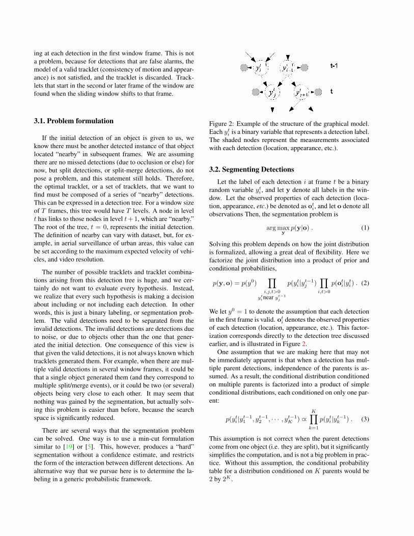
Figure 2: Example of the structure of the graphical model.Each yti is a binary variable that represents a detection label.The shaded nodes represent the measurements associatedwith each detection (location, appearance, etc.).

3.2. Segmenting Detections

Let the label of each detection i at frame t be a binaryrandom variable yti , and let y denote all labels in the win-dow. Let the observed properties of each detection (loca-tion, appearance, etc.) be denoted as ot

i, and let o denote allobservations Then, the segmentation problem is

argmaxy

p(y|o) . (1)

Solving this problem depends on how the joint distributionis formalized, allowing a great deal of flexibility. Here wefactorize the joint distribution into a product of prior andconditional probabilities,

p(y,o) = p(y0)∏

i,j,t>0

ytinear yt−1

j

p(yti |yt−1j )

∏i,t>0

p(oti|yti) . (2)

We let y0 = 1 to denote the assumption that each detectionin the first frame is valid. ot

i denotes the observed propertiesof each detection (location, appearance, etc.). This factor-ization corresponds directly to the detection tree discussedearlier, and is illustrated in Figure 2.

One assumption that we are making here that may notbe immediately apparent is that when a detection has mul-tiple parent detections, independence of the parents is as-sumed. As a result, the conditional distribution conditionedon multiple parents is factorized into a product of simpleconditional distributions, each conditioned on only one par-ent:

p(yti |yt−11 , yt−1

2 , · · · , yt−1K ) ∝

K∏k=1

p(yti |yt−1k ) . (3)

This assumption is not correct when the parent detectionscome from one object (i.e. they are split), but it significantlysimplifies the computation, and is not a big problem in prac-tice. Without this assumption, the conditional probabilitytable for a distribution conditioned on K parents would be2 by 2K .

Once the prior and conditional probabilities are speci-fied, the solution to the segmentation problem is given byMAP inference. In addition, the max-marginals provide uswith a confidence estimate of each detection. MAP infer-ence is a well-studied problem, and can be solved using themax-product algorithm [10] or LP relaxation algorithms,such as [16]. Note that the structure of the factorization willhave cycles in general, and as will be seen shortly, the con-ditional probability distributions, when viewed as energyfunctions, are not submodular, so the solution will be anapproximation.

The conditional probability p(oti|yti) reflects the appear-

ance similarity between the corresponding detection yti andthe initial detection y0. Any appearance similarity measurecan be used. It can be as simple as a sum of squared differ-ences, or as complex as output of a classifier. For appear-ance similarity a that ranges in [0, 1], the distribution is just

yti = 0 yti = 1p(ot

i|yti) 1− a(oti,o

0) a(oti,o

0)

The conditional probability p(yti |yt−1j ) is based on both

the appearance similarity between the corresponding de-tections, as well as the motion likelihood of this detectiongiven the preceding detections. The preceding detectionsare those which are on the path up to the root in the detec-tion tree. There is a problem with this definition when aparticular detection has multiple parents, because the mo-tion model, which is described below, assumes only oneobservation at each timestep. To solve this problem we takethe parent detection which gives the maximum motion like-lihood, and call it the “motion parent.” The effect of thisis not to unfairly penalize valid detections that follow thisambiguity. For a motion likelihood m that ranges in [0, 1],the conditional probability table is shown in Table 1.

This conditional distribution is a little bit complicateddue to the asymmetry. The asymmetry is necessary, becausewe need a different behavior when the parent label is 0 (in-valid detection) and when it is 1 (valid detection). When theparent detection is valid (bottom row), the distribution ex-presses that the probability is high when the detection labelappears similar to the parent, and the motion likelihood af-ter observing this detection is high (the motion is smooth).When the parent detection is invalid, however, we can notsay anything about the appearance similarity. This is be-

yti = 0 yti = 1yt−1j = 0 0.5 0.5yt−1j = 1 1− a(ot

i,ot−1j )m(ot

i) a(oti,o

t−1j )m(ot

i)

Table 1: Conditional probability distribution used in thegraphical model.

cause a parent detection that is a false alarm (noise) maystill have a similar appearance and motion. Therefore, inthis case the distribution does not give a “hint” about thelabel of the detection.

Any motion model can be used to determine the motionlikelihood. Here we use a simple linear-Gaussian model:

zt+1 = Azt + w (4)xt+1 = Hxt + v (5)

where zt+1 is the state vector, which includes the objectposition and velocity, xt+1 is the measurement vector of theobject position, w ∼ N (0,Q) is the process noise, and v ∼N (0,R) is the measurement noise. The motion likelihoodm is then

m(yti) = exp

(−1

2eTi P−1

i ei

)(6)

where ei = zit − zit and Pi = APiAT . zit is the poste-

rior state estimate, Pi is the prior state covariance, and Pi

is the posterior state covariance in the previous time step.The model is initialized using the first two detections in thesequence.

Having specified the joint distribution, the MAP labelingis given by MAP inference. As indicated earlier, the validdetections in this labeling do not always define one tracklet.There may be extra detections due to noise, limitations ofour model (a simplified factorization of the joint), the useof approximate inference, or when two objects with mergeddetections are splitting in this window. We describe how tohandle this problem next.

3.3. Tracklets from detections

One way to solve this problem is to generate possibletracklets (hypotheses), and find zero or more that best ex-plain the detections. Note that the search space is signif-icantly reduced than before the segmentation, as we onlyneed to explain the valid detections. Quite often there willbe only one hypothesis.

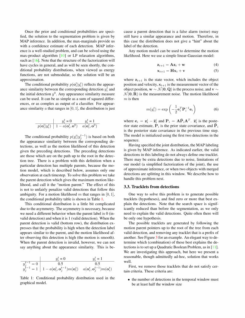
The possible tracklets are generated by following themotion parent pointers up to the root of the tree from eachvalid detection, and removing any tracklet that is a prefix ofanother. See Figure 3 for an example. An elegant way to de-termine which (combination) of these best explains the de-tections is to set up a Quadratic Boolean Problem, as in [11].We are investigating this approach, but here we present areasonable, though admittedly ad-hoc, solution that workswell.

First, we remove those tracklets that do not satisfy cer-tain criteria. These criteria are:

• the number of detections in the temporal window mustbe at least half the window size

Figure 3: Generating possible tracklets from valid detec-tions. Valid detections are denoted with thick outlines. Inthis case, two possible tracklets are generated as indicatedby the shaded regions.

• the average acceleration of the object must be less thana threshold (≈ 6m/s2)

• the object must be undergoing a smooth motion.

The average acceleration is estimated from the position ofthe detections, which are at least half a second apart. Theelapsed time requirement is necessary to avoid bad esti-mates due to discretization noise. To determine motionsmoothness for the third criterion, we compute the dot prod-uct of successive motion directions (at least half a secondapart), transform it to [0, 1] range, and compute the average.This average must be greater than a threshold (≈ 0.80) forthe criterion to be satisfied. Note that this does not rule outtracklets that are making a turn, since the large change indirection will be filtered out by the average.

Another criterion that may be useful in aerial surveil-lance is to require that the object moves with some mini-mum speed, or travels a minimum distance. The effect ofthis is to filter out motion due to parallax. This is not ap-plicable in all applications, however, so it is not includedabove. Other application-specific criteria can be defined.

The second step is to merge tracklets that are a resultof split-merge events. This is done by repeatedly mergingtracklets that have similar appearance and motion. Moreprecisely, the similarity of two tracks τ1 and τ2 is computedusing

sim(τ1, τ2) =1

T

T∑1

sim(τ1, τ2, t) (7)

sim(τ1, τ2, t) = a(τ t1, τt2) ∗ p(xt

1,xt2) ∗ v(vt

1,vt2) (8)

p(x1,x2) = exp(−‖x1 − x2‖/c) (9)v(v1,v2) = exp(−‖v1 − v2‖/c) , (10)

where a(·) is the appearance similarity measure as before,x is the position of the detection, p(·) is a distance measure,v is the velocity at the time of the detection, v(·) is veloc-ity similarity measure, and c is a constant to increase the

dynamic range (c ≈ 32). If the two tracklets share a detec-tion in a particular frame, the similarity is automatically 1for that frame, and if one tracklet has a detection in a frame,but the other one does not, a(·) is calculated using the previ-ous detection, and x, v are interpolated. When sim(τ1, τ2)exceeds a threshold (≈ 0.90), the two tracks are merged.

3.4. Occlusion handling

So far in the discussion we have assumed there is no oc-clusion or missing data. It turns out that when an object isoccluded but the occluder is detected, the algorithm as pre-sented still works. This is because the detection tree doesnot really change, except that no detections in the framewhere the object is occluded will be valid. A tracklet is stillfound, provided that the object is not occluded for most ofthe window. In that case, the tracklet would fail the firstcriterion above.

The real problem that needs to be handled is missing de-tections. When there is a missed detection, the detectiontree will be shorter than T . If it is too short, any track-lets that are found will not have enough detections and failthe first criterion above. This problem is solved by adding“virtual detections” to the detection tree. These are addedwhenever a detection in frame t has no nearby detectionsin frame t+ 1. The position of this virtual detection is esti-mated using the motion model, and the appearance is copiedfrom the (detected) parent. This procedure is recursive, sothat when a newly added virtual detection does not havenearby detections in the next frame, the process is repeated.

4. Multi-object trackingA multi-object tracker based on tracklets found by the

presented algorithm works as shown in Figure 1. The stepthat we now address is the second one – associating track-lets with existing tracks. The task of this step is to form longtracks from tracklets found in the sliding window. Manystrategies can be used here, but an important property tokeep in mind is the many-many mapping. When two ob-jects merge, and stay merged for a period longer than thewindow size, this association step must associate the onetracklet found with both existing tracks. Similarly, whenone object has split detections for a period longer than thewindow size, the tracklets found need to be associated withthe one existing track. Here we present one strategy thatallows a many-many mapping.

We proceed again by defining an association similaritymeasure, resembling (7):

sim2 (τ1, τ2) =1

T

T∑1

sim2 (τ1, τ2, t) (11)

sim2 (τ1, τ2, t) = a(τ t1, τt2) ∗ ps(xt

1,xt2) (12)

ps(x1,x2) = exp(−‖x1 − x2‖/c) . (13)

One difference here is that x is a vector containing the de-tection position as well as size. Also, if a track that we arecomparing to does not have a detection at a particular frame(there must be at least one such frame since the sliding win-dow shifted), the position of the detection is interpolated orextrapolated as necessary, and the appearance is taken fromthe most recent detection. This allows matching tracklets totracks across long sensor gaps, assuming the motion of theexisting track can be estimated accurately.

For a many-many mapping, we associate each trackletwith an existing track as long as sim2 is above a threshold.If we are only interested in matching each tracklet to one ex-isting track, then we associate with a track having the maxi-mum similarity, provided the similarity is above a threshold.In the latter case, a reasonable threshold is ≈ 0.40.

4.1. Implementation notes

We have implemented the algorithm just presented inC++. The implementation is available on the author’s web-site. The runtime of the algorithm depends on the numberof moving objects in the scene. When the number of ob-jects is small (≈ 50), the runtime is around 1-2 frames persecond on a 640x480 video. When the number of objects isin the hundreds, the runtime is several seconds per frame.Also, max-product was used for MAP inference.

5. Results

We have evaluated the multi-object tracker on sequencescaptured from an airborne sensor. The sequences comefrom the publicly available CLIF 2006 dataset [1]. Thevideo is captured at roughly 2 Hz, and it is in grayscale. Asthis is a large format video roughly 6600x7500 pixels, wechose 640x480 subregions over an expressway for the pur-poses of evaluation. The sequences were stabilized prior totracking. All of the sequences used in evaluation are avail-able for download.

The only moving objects in the video are vehicles, butthey are in very low resolution. Each vehicle is only about7x7 pixels, which makes detection and tracking quite chal-lenging. Since this low resolution gives very limited ap-pearance information, we used a simple sum of squareddifferences function as our appearance similarity. This iscomputed after doing a least-squares alignment of the twoimage patches. The alignment is parameterized by transla-tion and rotation. In this context, this parameterization issatisfactory.

The moving object detection was done using backgroundsubtraction. The background is modeled as the mode of a(stabilized) sliding window of frames. We have also tried amixture of Gaussian model, but we did not see a significantdifference. A window size of 16 frames, corresponding toabout 8 seconds of video was used.

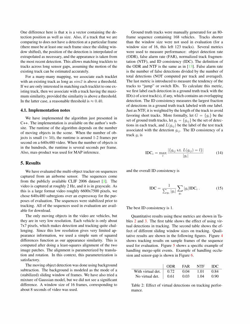
Ground truth tracks were manually generated for an 80-frame sequence containing 168 vehicles. Tracks shorterthan the window size were not used in evaluation (for awindow size of 16, this left 123 tracks). Several metricswere used to measure performance: object detection rate(ODR), false alarm rate (FAR), normalized track fragmen-tation (NTF), and ID consistency (IDC). The definition ofthe ODR and NTF is the same as in [13]. False alarm rateis the number of false detections divided by the number oftotal detections (NOT computed per track and averaged).The last metric is introduced to measure the tendency of thetracks to “jump” or switch IDs. To calculate this metric,we first label each detection in a ground truth track with theID(s) of a test track(s), if any, which contains an overlappingdetection. The ID consistency measures the largest fractionof detections in a ground truth track labeled with one label.Just as NTF, it is weighted by the length of the track to avoidfavoring short tracks. More formally, let G = {gi} be theset of ground truth tracks, let gi = {gij} be the set of detec-tions in each track, and L(gij) be the label of the test trackassociated with the detection gij . The ID consistency of atrack gi is

IDCi = maxl

|{gij s.t. L(gij) = l}||gi|

(14)

and the overall ID consistency is

IDC =1∑

gi|gi|

∑gi

|gi|IDCi . (15)

The best ID consistency is 1.

Quantitative results using these metrics are shown in Ta-bles 2 and 3. The first table shows the effect of using vir-tual detections in tracking. The second table shows the ef-fect of different sliding window sizes on tracking. Quali-tative results are shown in the following figures. Figure 4shows tracking results on sample frames of the sequenceused for evaluation. Figure 5 shows a specific example ofhandling merge-split events. Example of handling occlu-sion and sensor-gap is shown in Figure 6.

ODR FAR NTF IDCWith virtual det. 0.72 0.04 1.01 0.84No virtual det. 0.61 0.03 1.04 0.90

Table 2: Effect of virtual detections on tracking perfor-mance.

Figure 4: Tracking results on sequence 1. A green box denotes a real detection, whereas a yellow box denotes an interpolateddetection.

(a) Frame 38 (b) Frame 46 (c) Frame 51

Figure 5: Example of merge event handling. Other tracksare not shown for clarity.

(a) Frame 49 (b) Frame 51 (c) Frame 54

Figure 6: Example of occlussion handling.

Window Sz. ODR FAR NTF IDC10 0.76 0.04 1.06 0.8612 0.73 0.04 1.00 0.8514 0.72 0.04 1.00 0.8716 0.72 0.04 1.01 0.8418 0.71 0.05 1.00 0.8320 0.63 0.04 1.00 0.89

Table 3: Effect of sliding window size on tracking per-formance.

(a) Frame 8 (b) Frame 10 (c) Frame 13

Figure 7: Example of a temporary ID switch. Other tracksare not shown for clarity.

5.1. Discussion

It is clear from the quantitative evaluation that the algo-rithm presented is very good at making detection associa-tions. This is supported by the track fragmentation score,which is nearly perfect, as well as the ID consistency score.Once a track is established, tracking is unlikely to stop pre-maturely. The ID consistency score indicates that while it ispossible that during tracking the ID may switch to anotherobject, it is only a temporary change, as it never results inthe original track being fragmented. An example of this canbe seen in Figure 7.

Given the challenging nature of the video sequence, theobject detection rate is quite good. Many of the detectionfailures are due to poor contrast between the object and thebackground. Another factor limiting the detection rate isthe appearance similarity function. In our experiments weused sum of squared differences, which worked well, butthere were cases where the alignment of two image patchesdid not converge correctly, and the computed similarity waslow. However, thanks to the use of a sliding window andvirtual detections, a missed detection in one frame does not

cause the tracking to fail.As a matter of fact, virtual detections are critical to

achieving high object detection rate. Table 2 indicates thatthe object detection performance drops significantly whenvirtual detections are not used. It also shows that the falsealarm rate slightly increases, however, it is more than com-pensated for the increased object detection rate.

The sliding window size mainly affects the object detec-tion rate. As the sliding window size increases, more de-tections are necessary in order to declare a potential trackvalid. We would expect the false alarm rate to increase withdecreasing window size, although it is not evident in the se-quence used in evaluation. The false alarm rate is very low,despite some parallax motion due to buildings and trees inthe scene.

6. Conclusions

Our primary contribution is a new algorithm for deter-mining tracklets in a window of frames. This is a large dataassociation problem between detections and an unknownnumber of objects, which we solve using inference in a setof Bayesian networks. Exhaustive evaluation of data associ-ation hypotheses is avoided, while allowing for split-mergeconditions. The separation of valid detections from invaliddetections is optimal in a MAP sense. In addition, we get aconfidence estimate of each detection.

The algorithm was evaluated on a vehicle tracking task inan aerial surveillance video. The results show excellent per-formance in terms of object detection rate, track fragmenta-tion, and false alarm rate on challenging video sequences.

We are currently working on a principled way to deter-mine tracklets from valid detections using the QuadraticBoolean Problem. One avenue for future research is de-veloping a more robust structure of the inference problemusing higher-order relationships instead of using just pair-wise. Another possible extension is to take advantage ofother, application-specific, sources of information by incor-porating them into the graphical model. For example, in thecase of aerial surveillance, this can be a road network.

7. Acknowledgements

This work was supported in part by grant DE-FG52-08NA28775 from the U.S. Department of Energy. For thesecond author, this work was prepared by Lawrence Liver-more National Lab under contract DE-AC52-07NA27344.

References[1] CLIF 2006. https://www.sdms.afrl.af.mil/. 6[2] M. Andriluka, S. Roth, and B. Schiele. People-tracking-by-

detection and people-detection-by-tracking. In IEEE Con-ference on CVPR, pages 1–8, 2008. 1

[3] I. Cox and S. Hingorani. An efficient implementation ofreid’s multiple hypothesis tracking algorithm and its evalu-ation for the purpose of visual tracking. IEEE Transactionson PAMI, 18(2):138–150, Feb 1996. 2

[4] T. Fortmann, Y. Bar-Shalom, and M. Scheffe. Sonar trackingof multiple targets using joint probabilistic data association.Oceanic Engineering, IEEE Journal of, 8(3):173–184, Jul1983. 2

[5] D. Greig, B. Porteous, and A. Seheult. Exact maximum aposteriori estimation for binary images. Journal of the RoyalStatistical Society, 51(2):271–279, 1989. 3

[6] C. Huang, B. Wu, and R. Nevatia. Robust object tracking byhierarchical association of detection responses. In EuropeanConference on Computer Vision, pages 788–801, 2008. 1, 2

[7] H. Jiang, S. Fels, and J. Little. A linear programming ap-proach for multiple object tracking. In IEEE Conference onCVPR, pages 1–8, 2007. 2

[8] S. L. Junlian Xing, Haizhou Ai. Multi-object trackingthrough occlusions by local tracklets filtering and globaltracklets association with detection responses. In IEEE Con-ference on CVPR, pages 1200–1207, 2009. 1, 2

[9] Z. Khan, T. Balch, and F. Dellaert. Multitarget tracking withsplit and merged measurements. In IEEE Conference onCVPR, volume 1, pages 605–610, 2005. 2

[10] F. Kschischang, B. Frey, and H.-A. Loeliger. Factor graphsand the sum-product algorithm. Information Theory, IEEETransactions on, 47(2):498–519, Feb 2001. 4

[11] B. Leibe, E. Seemann, and B. Schiele. Pedestrian detectionin crowded scenes. In IEEE Conference on Computer Visionand Pattern Recognition, volume 1, pages 878–885, 2005. 4

[12] K. Okuma, A. Taleghani, N. de Freitas, J. Little, andD. Lowe. A boosted particle filter: Multitarget detection andtracking. In ECCV, volume 3021 of LNCS, pages 28–39,2004. 2

[13] A. Perera, C. Srinivas, A. Hoogs, G. Brooksby, and W. Hu.Multi-object tracking through simultaneous long occlusionsand split-merge conditions. In IEEE Conference on CVPR,volume 1, pages 666–673, 2006. 1, 2, 6

[14] D. Reid. An algorithm for tracking multiple targets. Auto-matic Control, IEEE Transactions on, 24(6):843–854, Dec1979. 2

[15] V. Reilly, H. Idrees, and M. Shah. Detection and tracking oflarge number of targets in wide area surveillance. In ECCV,volume 6313 of LNCS, pages 186–199. 2010. 1

[16] D. Sontag, T. Meltzer, A. Globerson, T. Jaakkola, andY. Weiss. Tightening lp relaxations for map using messagepassing. 2008. 4

[17] A. Yilmaz, O. Javed, and M. Shah. Object tracking: A sur-vey. ACM Comput. Surv., 38(4):13, 2006. 1

[18] Q. Yu and G. Medioni. Multiple-target tracking by spa-tiotemporal monte carlo markov chain data association.IEEE Trans. on PAMI, 31(12):2196–2210, Dec. 2009. 2

[19] L. Zhang, Y. Li, and R. Nevatia. Global data association formulti-object tracking using network flows. In IEEE Confer-ence on CVPR, pages 1–8, 2008. 2, 3