Inferring phylogeny - National Taiwan Universityhomepage.ntu.edu.tw/~ctting/CMB_files/Phylogeny...

Inferring phylogeny

Introduction ! Distance methods ! Parsimony method

!"#$%&'(!)*

+,-

.'/01!23454(6!7!2845*0&4'9#6!:&454(6

;<=>?@AB=C?DEF

1

Today’s topics

Overview of phylogenetic inferences

Methodology

Methods using distance data

UPGMA, Neighbor-joining, minimum evolution

Methods using discrete data

Maximum parsimony

Maximum likelihood

Bayesian inference

2

Milestones of molecular evolution studies1800 1900 2000

First example of molecular systematics: Vince Sarich & Allan Wilson (1967) on human evolution

Nature (1968) 217: 624

Genetics: Gregor Mendel (1856-1863)

Origin of species: Charles Darwin (1859)

Discovery of DNA structure: James Watson & Francis Crick (1953)

First comparison of amino acid sequence (insulin) among different species: Fred Sanger et al. (1955)

Technical breakthrough in the 1980s: PCR, DNA sequencing, etc.

Technical breakthrough in the 1990s: computer speed, methodological improvement

Emergence of cladistics: Willi Hennig et al. The blooming of

evo devo studies

33

Contributions to molecular evolution

The models and methodological concerns

Cladistics and phylogenetics:

Willi Hennig (1913-1976)

The neutral theory of molecular evolution:

Motoo Kimura (!"#$, 1924-1994)

The mechanisms

The patterns of evolution

The uses of parsimony, maximum likelihood methods in phylogenetics:

Joseph Felsenstein

Genome Science and of Biology, University of Washington, Seattle

The neutral theory of molecular evolution 4

Reconstructing phylogeny

The concepts of trees

The data used to construct phylogenetic trees

Morphological data

Molecular data

Homology of characters in data matrices

Sequence alignment

55

The basics of evolutionary trees

The tree shapes

Baum et al. (2005) Science 310:979

Are these two trees different?

66

Plant Molecular Evolution

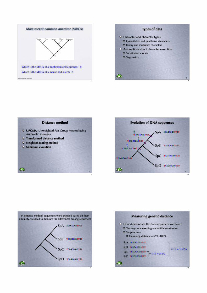
Most recent common ancestor (MRCA)

Which is the MRCA of a mushroom and a sponge?

Which is the MRCA of a mouse and a fern?

d

b

7

Types of data

Character and character types

Quantitative and qualitative characters

Binary and multistate characters

Assumptions about character evolution

Substitution models

Step matrix

88

Distance method

UPGMA (Unweighted Pair Group Method using Arithmetic averages)

Transformed distance method

Neighbor-Joining method

Minimum evolution

99

Evolution of DNA sequences

SpA

SpB

SpC

SpD TCAGACGACTGT

TCAGACGACTGT

TCAGCCGACTGT

TCAGACGACTGT

C TCAGCCGATTGT

TCAGCCGACTGT

T

ACAGCCGATTGT

TCAGCCGACTGT

A

1010

In distance method, sequences were grouped based on their similarity, we need to measure the differences among sequences

SpA

SpB

SpC

SpD TCAGACGACTGT

TCAGCCGACTGT

TCAGCCGATTGT

ACAGCCGATTGT

11

Measuring genetic distance

How different are the two sequences we have?

The ways of measuring nucleotide substitution

Simplest way

Hamming distance = n/N x100%

SpA

SpB

SpC

SpD TCAGACGACTGT

TCAGCCGACTGT

TCAGCCGA-TGT

ACAGCCGA-TGT

1/12 = 8.3%

2/12 = 16.6%

12

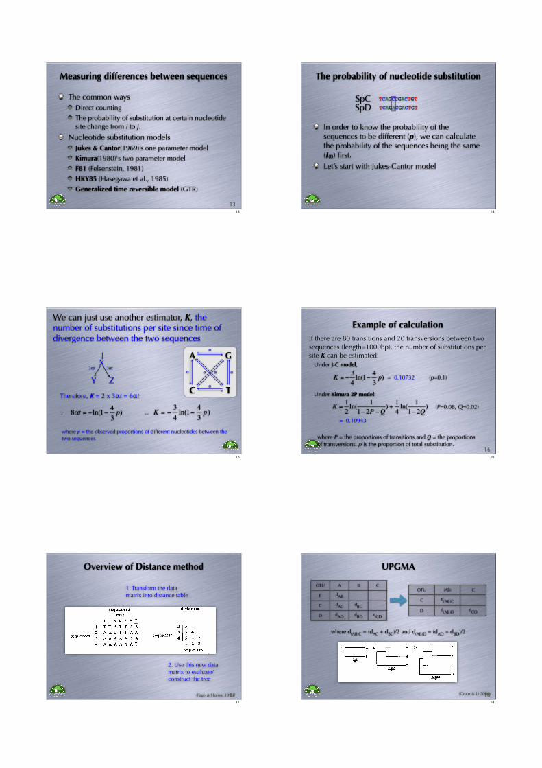
Measuring differences between sequences

The common ways

Direct counting

The probability of substitution at certain nucleotide site change from i to j.

Nucleotide substitution models

Jukes & Cantor(1969)’s one parameter model

Kimura(1980)'s two parameter model

F81 (Felsenstein, 1981)

HKY85 (Hasegawa et al., 1985)

Generalized time reversible model (GTR)

1313

The probability of nucleotide substitution

SpCSpD TCAGACGACTGT

TCAGCCGACTGT

In order to know the probability of the sequences to be different (p), we can calculate the probability of the sequences being the same (I(t)) first.

Let’s start with Jukes-Cantor model

14

X

Y Z

We can just use another estimator, K, the number of substitutions per site since time of divergence between the two sequences

3"t

A G

C T

"

"

"" " "

3"t

Therefore, K = 2 x 3"t = 6"t

K = !3

4ln(1!

4

3p)8!t = "ln(1"

4

3p)! "

where p = the observed proportions of different nucleotides between the two sequences

15

Example of calculation

Under J-C model,

Under Kimura 2P model:

K =1

2ln(

1

1! 2P !Q) +1

4ln(

1

1! 2Q)

where P = the proportions of transitions and Q = the proportions of transversions. p is the proportion of total substitution.

K = !3

4ln(1!

4

3p)

16

If there are 80 transitions and 20 transversions between two sequences (length=1000bp), the number of substitutions per site K can be estimated:

= 0.10732 (p=0.1)

(P=0.08, Q=0.02)

= 0.10943

16

Overview of Distance method

(Page & Holme 1998)

2. Use this new data matrix to evaluate/construct the tree

1. Transform the data matrix into distance table

1717

UPGMA

OTU A B C

B dAB

C dAC

dBC

D dAD

dBD

dCD

OTU (AB) C

C d(AB)C

D d(AB)D

dCD

where d(AB)C = (dAC + dBC)/2 and d(AB)D = (dAD + dBD)/2

(Graur & Li 2000)1818

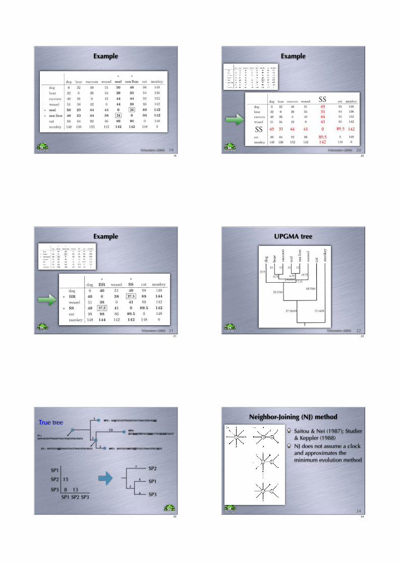
Example

Felsenstein (2004) 1919

Example


Example


UPGMA tree


SP1: AAACGCGCTTAGATCGCCTAACGTACAAGC

N1:

AATCGCGCTTAGATCGCCTAACGTACAACG

N2: AATCGCGGGTAGATCGCCTAACGTACAACG SP3: AATCGCGGGTATTTCGCCTAACGTACATCG

SP2: TATAAAGGGTAGAAAACCTAAGGATCAACG

True tree

15

8 13

SP1 SP2 SP3

SP1

SP2

SP3

3

2

3

10

SP2

SP1

SP3

7

4

4

3

23

Neighbor-Joining (NJ) method

Saitou & Nei (1987); Studier & Keppler (1988)

NJ does not assume a clock and approximates the minimum evolution method

2424

2. Choose the i and j for which Dij-ui-uj

is smallest

1. For each tip, compute

ui =Di

(n ! 2)j: j" i

n

#

3. Join i and j, compute the new node

(ij) to every other nodes

4. Delete tips i and j and make new table with the new node (ij)

5. Continue till resolve the tree

25

D(ij ),k =

(Dik + Djk !Dij )

2

NJ procedure

25

Limitation on distance methods

All nucleotide sites change independently.

When evolutionary rates vary from site to site, than the data set needs to be corrected

The substitution rate is constant over time and in different lineages.

The base composition is at equilibrium.

The conditional probabilities of nucleotide substitutions are the same for all sites and do not change over time.

2626

Discrete methods

Maximum parsimony (%&'()*)

Maximum likelihood (+,-./)*)

Bayesian inference (01234567)

Others

27

Parsimony methods

The goal is to find the most parsimonious tree

The criteria are to calculate the changes of character states, i.e. the evolutionary steps

First, we have to know the way to evaluate a given tree

2828

A simple data matrix w/ discrete characters

SpA SpB SpC SpD SpA SpB SpD SpC SpA SpC SpD SpB

SpA: TCAGACGATTGTCAGACCATTG

SpB: TCAGTCGACTGTCAAACCATTG

SpC: TCGGTCAATTGTCAAACGATTG

SpD: TCGGTCAATTGTCAAACGATTG

2929

A simple data matrix w/ discrete charactersSpA: TCAGACGATTGTCAGACCATTG





For position no. 3

Character change (step) = 2

A A G G A A G G A AGG


A to G


30

SpA SpB SpC SpD

A A G G

30






For position no. 7


A AG G


G to A


A AG G AAG G

3131







A AG G

Character change (step) = 9 Character change (step) = 6

A AG G AAG G

3232

Consensus trees

Finding the underlying information among trees

(Page & Holme 1998)3333

So, how many trees out there are we dealing with?

3434

3 taxa

4 taxa

3535

Tree searching

Nunrooted

=(2n ! 5)!

2n!3(n ! 3)!

Nrooted

=(2n ! 3)!

2n!2(n ! 2)!

The number of unrooted trees:

The number of rooted trees:

3636

Taxon number All possible unrooted tree number

3 1

4 3

5 15

6 105

7 945

8 10,395

9 135,135

10 2,027,025

11 34,459,425

12 654,729,075

13 13,749,310,575

14 316,234,143,225

15 7,905,853,580,625

16 213,458,046,676,875

17 6,190,283,353,629,375

18 191,898,783,962,510,625

19 6,332,659,870,762,850,625

20 221,643,095,476,699,771,875

21 8,200,794,532,637,891,559,375

22 319,830,986,772,877,770,815,625

23 13,113,070,457,687,988,603,440,625

24 563,862,029,680,583,509,947,946,875

25 25,373,791,335,626,257,947,657,609,375 >1029

... etc. 3737

Note

We got to have some ways to approximate the true tree.

Say a computer can evaluate 106 trees per second.

If we want to evaluate all of the trees for 25 taxa, we will need

x = 1029/106/60/60/24/365 = 3.17x1015!"#$%!&

3838

Ways to solve time paradigm

Skip unnecessary calculation

Change the tree searching ways

3939

The procedure can be simplified

SpA: TCAGACGATTGTCAGACCATTG

SpB: TCGGTCGACTGTCAGACCATTG

SpC: TCAGTCGATTGTCA-ACGATTG

SpD: TCAGTCGATTGTCA-ACGATTG

SpE: TCAGTCGATCGTCA-ACGATTG

Parsimonious uninformative

Parsimonious informative

4040

Searching for optimal trees

Exhausted search

Branch-and-bound method

Heuristic approach

Stepwise/closest/random addition

Star decomposition

Branch swapping

4141

Exhausted search

Page & Holme (1998) Molecular evolution

42

Distribution of tree lengthFrequency distribution of lengths of 1000000 random trees:

mean=6528.095481 sd=65.005662 g1=-0.322317 g2=0.1598486114.00000 /---------------------------------------------------------------------6146.30000 | (1)6178.60000 | (3)6210.90000 | (24)6243.20000 | (84)6275.50000 | (302)6307.80000 | (1071)6340.10000 |# (3493)6372.40000 |### (9300)6404.70000 |######## (22649)6437.00000 |################# (48576)6469.30000 |################################# (94873)6501.60000 |################################################## (144323)6533.90000 |################################################################# (187000)6566.20000 |##################################################################### (199355)6598.50000 |##################################################### (153445)6630.80000 |############################### (88764)6663.10000 |############# (36489)6695.40000 |### (8865)6727.70000 | (1266)6760.00000 | (117) \---------------------------------------------------------------------

Data of bird ovomucoids

43

Tree-island profile: First Last First TimesIsland Size tree tree Score replicate hit---------------------------------------------------------------------- 1 101 1471 1571 3890 3 1 2 69 4961 5029 3890 10 1 3 1 14236 14236 3890 30 1 4 5 14237 14241 3890 31 1 5 1236 1 1236 3891 1 2 6 96 8816 8911 3891 20 1 7 256 9524 9779 3891 23 2 8 960 14242 15201 3891 32 2 9 624 15202 15825 3891 33 1 10 3085 15870 18954 3891 37 1 11 1488 1911 3398 3892 5 1 12 626 3448 4073 3892 7 2 13 211 4074 4284 3892 8 1 14 96 5935 6030 3892 12 1 15 156 7211 7366 3892 14 2 16 236 7367 7602 3892 15 2 17 1053 7667 8719 3892 18 1 18 291 9780 10070 3892 24 1 19 576 10071 10646 3892 25 1 20 96 18987 19082 3892 39 1 21 676 4285 4960 3893 9 1 22 905 5030 5934 3893 11 1 23 96 8720 8815 3893 19 1 24 612 8912 9523 3893 21 1 25 32 18955 18986 3893 38 1 26 18 19083 19100 3893 40 1 27 339 1572 1910 3894 4 2 28 64 7603 7666 3894 17 1 29 3589 10647 14235 3894 26 1 30 234 1237 1470 3895 2 1 31 49 3399 3447 3895 6 1 32 44 15826 15869 3895 35 1 33 1180 6031 7210 3896 13 1

Data of bird ovomucoids

Results of heuristic search, with random addition from

random starting points

44

Branch and bound searching

Hendy & Penny (1982) first used this method for inferring phylogenies.

An example - shortest Hamiltonian path (SHP)

For n cities, there will be n-1 cities to come next, so there will be n! possible solution

Hendy, M.D. & D. Penny (1982) Mathem. Biosci. 60: 133-142.

Felsenstein (2004) Inferring phylogeny4545

A shortest Hamiltonian path problem

Felsenstein (2004) Inferring phylogeny

Random route:Total length=5.4342

Point x y

1 0.537 0.061

2 0.274 0.222

3 0.016 0.837

4 0.871 0.400

5 0.399 0.740

6 0.815 0.531

7 0.587 0.946

8 0.992 0.733

9 0.268 0.481

10 0.895 0.068

Adding by greedy manner:Length=2.8027

Optimal solution:Length=2.7812

4646

Branch-and-bound search

Page & Holme (1998) Molecular evolution

#This method can greatly

improve the speed of search, but it still cannot escape from the constraints of the NP-hardness proof.

4747

heuristic searching for best tree


Nearest-neighbor

interchanges (NNI)

Heuristic approach- Branch swapping: NNIs

Swofford et al. (1996) Molecular Systematics4949

How greedy should we be?

In a tree with n tips, there will be n-3 interior branches.

In all, 2(n-3) neighbors will be examined for each tree.

Should we do NNI for each of the best trees, or stop at some point, or should we start from scratch more often?

5050

The space of all 15 possible unrooted trees


The space of all 15 possible unrooted trees

Felsenstein (2004) Inferring phylogeny

NNI is to moving in this graph

5252

Heuristic approach- Branch swapping: TBR

Tree bisection and reconnection (TBR)

Swofford et al. (1996) Molecular Systematics

In a n1+n2 species in the tree, there will

be (2n1-3)(2n2-3) possible ways to

reconnect the two trees.

5353

Browsing tree space

Maddison, D.R. (1991) Syst. Zool. 40: 315-328.Nixon, K.C. (1999) Cladistics 15: 407-414.

Rearrangement

Random starting point strategy to avoid being trapped in “tree island” (Maddison 1991)

Parsimony ratchet

Parsimony ratchet uses a re-weighted subset of characters as a starting point to browse the tree space, and tries to find as many tree islands as possible by using adjacent-tree searching method. (Nixon 1999)

5454

Parsimony ratchet

Described by Nixon (1999), and available in various programs (NONA, WINCLADA, PAUPRat, etc.).

Parsimony ratchet uses a re-weighted subset of characters as a starting point to browse the tree space, and tries to find as many tree islands as possible by using adjacent-tree searching method.

Nixon, K.C. (1999) Cladistics 15: 407-414.

5555

Parsimony ratchet procedure

Generate a starting “Wagner” tree

Randomly select a subset of character (5-25%) and add 1 weight score

Performing TBR branch swapping, keep 1 tree

Reset the weighting to original

Performing branch swapping, keep the best tree

Return to step 2, repeat the iteration (step2-6) 50-200 times

5656

Nixon, K.C. (1999) Cladistics 15: 407-414.5757

Notes on parsimony ratchet

It seems to improve the effectivity of tree searching

It can be used with any objective function based on character data: compatibility, distance matrix, and likelihoods.

The strategy can be modified

5858

Weighted parsimony method

Incorporating simple nucleotide models into MP analysis

Transition vs. transversion scores

A C G T

A 0 2.5 1 2.5

C 2.5 0 2.5 1

G 1 2.5 0 2.5

T 2.5 1 2.5 0

59

The Sankoff algorithm applied to the tree

0! ! ! 0 ! ! ! 0! ! ! 0 ! ! ! 0!! !

2.52.5 3.5 3.5

3.5 3.5 3.5 4.5

1 5 1 5

6 6 7 8

C A C A G

CA G T

A C G T

A 0 2.5 1 2.5

C 2.5 0 2.5 1

G 1 2.5 0 2.5

T 2.5 1 2.5 0

Modified from Felsenstein (2004) Inferring phylogeny

S = min S0(i)

6060

How do we know the tree we got is right?

The evaluation

61

Evaluating trees

Character properties (CI, RI)Examining how “clean” is the data on a given tree

Confidence level of treesComparisons between obtained trees

Partition distance

Kishino-Hasegawa test

Distance test

Likelihood ratio test

Bootstrap/jackknife (internal support)

Bremer support (for parsimony)

6262

Properties of characters

Consistency index (CI) of each character is:

Tree CI for all characters in a specific tree:

character CI = mi/Si

mi

i=1

n

! wi

wi

i=1

n

! si

tree CI =

mi ='()*+,-./i01/23)*+,45 (minimum conceivable steps)

Si =06+,-./i01/+,45

wi = i01/789n:01;

6363

Properties of characters

Retention index (RI) of each characters is:

character RI = M

i! s

i

Mi! m

i

mi ='()*+,-./i01/23)*+,45 (minimum conceivable steps)

Mi ='()*+,-./i01/2<)*+,45 (maximum conceivable steps)

Si =06+,-./i01/+,45

6464

Example: calculating CI & RI

Taxon1 0 0 0 0Taxon2 0 0 0 1Taxon3 1 1 0 1Taxon4 1 1 1 1Taxon5 1 1 0 1

Character(1) CI=1/1=1Character(1) RI=(2-1)/(2-1)=1

Taxon2 0

Taxon3 1

Taxon4 1

Taxon1 0

Taxon5 1

Taxon4 1

Taxon3 1

Taxon2 0

Taxon1 0

Taxon5 1

Character CI=1/2=0.5Character RI=(2-2)/(2-1)=0

Tree 1 Tree 2

TreeCI =1+1+1+1

1+1+1+1=1 TreeCI =

1+1+1+1

2 + 2 +1+1= 0.67

6565

Evaluating trees

Character properties (CI, RI)

Confidence level of trees

Comparisons between obtained trees

Bootstrap/jackknife (internal support)

Bremer support (for parsimony)

6666

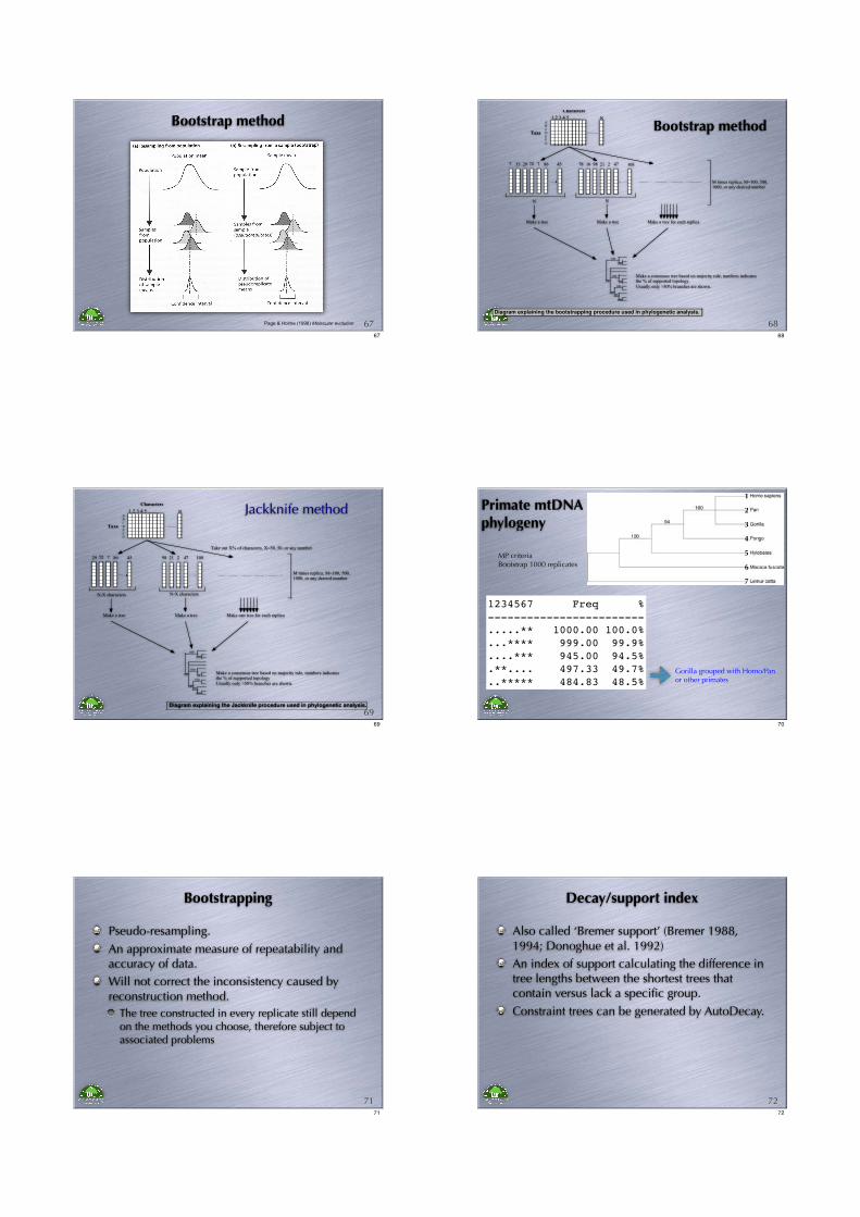
Bootstrap method

Page & Holme (1998) Molecular evolution 6767

1 2 3 4 5 ........ N

N

7 33 29 72 7 86 45

N

2116 9878 2 47 108

M times replica; M=100, 500,1000, or any desired number

Characters

Taxa

AB

CDEFG

Make a tree Make a tree Make a tree for each replica

100

100

100

100

100

100

100

99

86

Make a consensus tree based on majority rule, numbers indicatesthe % of supported topology.

Usually only >50% branches are shown.

Diagram explaining the bootstrapping procedure used in phylogenetic analysis.

Bootstrap method

6868

1 2 3 4 5 ........ N

N-X characters

29 72 7 86 45

N-X characters

2198 2 47 108

M times replica; M=100, 500,1000, or any desired number

Characters

Taxa

AB

CDEFG

Make a tree Make a tree Make one tree for each replica

100

100

100

100

100

100

100

99

86

Make a consensus tree based on majority rule, numbers indicatesthe % of supported topology

Usually only >50% branches are shown.

Diagram explaining the Jackknife procedure used in phylogenetic analysis.

Take out X% of characters, X=30, 50, or any number

Jackknife method

6969

Primate mtDNA phylogeny

1234567 Freq %

------------------------

.....** 1000.00 100.0%

...**** 999.00 99.9%

....*** 945.00 94.5%

.**.... 497.33 49.7%

..***** 484.83 48.5%

MP criteriaBootstrap 1000 replicates 6

7

5

4

3

2

1

Gorilla grouped with Homo/Pan or other primates

70

Bootstrapping

Pseudo-resampling.

An approximate measure of repeatability and accuracy of data.

Will not correct the inconsistency caused by reconstruction method.

The tree constructed in every replicate still depend on the methods you choose, therefore subject to associated problems

7171

Decay/support index

Also called ‘Bremer support’ (Bremer 1988, 1994; Donoghue et al. 1992)

An index of support calculating the difference in tree lengths between the shortest trees that contain versus lack a specific group.

Constraint trees can be generated by AutoDecay.

7272

Method of calculation

1. Obtain most parsimonious tree(s) (MP)

Generate a strict consensus tree

2. Obtain all trees one step longer (MP + 1)


If branch is not supported, Decay index = 1







7373

Bremer Support (decay index)

the number of extra steps it takes to collapse a group

example: 1 MP tree, 110 steps

Haliperp HPE232926

Arabaren AAU43231

Arabsuec ASU43227

Arabthal ATU43224

Arabsuec ASU43226

Arabthal ATH232900

Capsrube CRU232912

Capsrube CRU232913

7474


3 trees <= 111 steps

75

Haliperp HPE232926

Arabaren AAU43231

Arabsuec ASU43227

Arabthal ATU43224

Arabsuec ASU43226

Arabthal ATH232900

Capsrube CRU232912

Capsrube CRU232913

75



76

Haliperp HPE232926

Arabaren AAU43231

Arabsuec ASU43227

Arabthal ATU43224

Arabsuec ASU43226

Arabthal ATH232900

Capsrube CRU232912

Capsrube CRU232913

76



77

Haliperp HPE232926

Arabaren AAU43231

Arabsuec ASU43227

Arabthal ATU43224

Arabsuec ASU43226

Arabthal ATH232900

Capsrube CRU232912

Capsrube CRU232913

77


Can not be larger than the branch length

No direct connection to branch length otherwise

Quantification of support in a parsimony framework

6

13

12

10

13

15

26

78

Haliperp HPE232926

Arabaren AAU43231

Arabsuec ASU43227

Arabthal ATU43224

Arabsuec ASU43226

Arabthal ATH232900

Capsrube CRU232912

Capsrube CRU232913

78

Methodological concerns

Sampling problem

Performance of phylogenetic methods under computer simulation

79

Effects of sampling

(Page & Holmes, 1998)

0 change 3 changes

Makes No.2 a fast evolving taxon

8080

Long branch attraction

Joe Felsenstein (1978, Syst. Zool. 27: 401-410)

Page & Holme (1998) Molecular evolution8181

Simulation analysis

UPGMA Parsimony


Equal rate of evolution


Unequal rate of evolution


Parsimony

Weighted

parsimony

UPGMA

Lake!s invariants

Maximum likelihood(Jukes-Cantor)

Maximum likelihood(Kimura)

Weighted least squares

Swofford et al. (1996) Molecular Systematics8585

References of phylogenetics

Graur, D. and W.-H. Li. 2000. Fundamentals of Molecular Evolution. 2nd ed., Sinauer Assoc., Sunderland, MA, USA.

Hall, B. G. 2004. Phylogenetic trees made easy: a how-to manual, 2nd ed. Sinauer Assoc., Sunderland, MA.

Hillis, D. M., C. Moritz, and B. K. Mable (eds) 1996. Molecular systematics. Sinauer Assoc., Sunderland, MA.

Page, R. D. M., and E. C. Holmes. 1998. Molecular evolution - A phylogenetic approach. Blackwell Science Ltd, Oxford, the United Kingdom.

Yang, Z. H. 2006. Computational molecular evolution. Oxford University Press.

8686

Inferring phylogeny - National Taiwan Universityhomepage.ntu.edu.tw/~ctting/CMB_files/Phylogeny...

Documents

Transcript of Inferring phylogeny - National Taiwan Universityhomepage.ntu.edu.tw/~ctting/CMB_files/Phylogeny...