Inference with Difference-in-Differences Revisitedftp.iza.org/dp7742.pdf · Inference with...
38
DISCUSSION PAPER SERIES Forschungsinstitut zur Zukunft der Arbeit Institute for the Study of Labor Inference with Difference-in-Differences Revisited IZA DP No. 7742 November 2013 Mike Brewer Thomas F. Crossley Robert Joyce
Transcript of Inference with Difference-in-Differences Revisitedftp.iza.org/dp7742.pdf · Inference with...
DI
SC
US
SI
ON
P
AP
ER
S
ER
IE
S
Forschungsinstitut zur Zukunft der ArbeitInstitute for the Study of Labor
Inference with Difference-in-Differences Revisited
IZA DP No. 7742
November 2013
Mike BrewerThomas F. CrossleyRobert Joyce

Inference with Difference-in-Differences
Revisited
Mike Brewer University of Essex,
Institute for Fiscal Studies and IZA
Thomas F. Crossley University of Essex
and Institute for Fiscal Studies
Robert Joyce Institute for Fiscal Studies
Discussion Paper No. 7742 November 2013
IZA
P.O. Box 7240 53072 Bonn
Germany
Phone: +49-228-3894-0 Fax: +49-228-3894-180
E-mail: [email protected]
Any opinions expressed here are those of the author(s) and not those of IZA. Research published in this series may include views on policy, but the institute itself takes no institutional policy positions. The IZA research network is committed to the IZA Guiding Principles of Research Integrity. The Institute for the Study of Labor (IZA) in Bonn is a local and virtual international research center and a place of communication between science, politics and business. IZA is an independent nonprofit organization supported by Deutsche Post Foundation. The center is associated with the University of Bonn and offers a stimulating research environment through its international network, workshops and conferences, data service, project support, research visits and doctoral program. IZA engages in (i) original and internationally competitive research in all fields of labor economics, (ii) development of policy concepts, and (iii) dissemination of research results and concepts to the interested public. IZA Discussion Papers often represent preliminary work and are circulated to encourage discussion. Citation of such a paper should account for its provisional character. A revised version may be available directly from the author.

IZA Discussion Paper No. 7742 November 2013
ABSTRACT
Inference with Difference-in-Differences Revisited* A growing literature on inference in difference-in-differences (DiD) designs with grouped errors has been pessimistic about obtaining hypothesis tests of the correct size, particularly with few groups. We provide Monte Carlo evidence for three points: (i) it is possible to obtain tests of the correct size even with few groups, and in many settings very straightforward methods will achieve this; (ii) the main problem in DiD designs with grouped errors is instead low power to detect real effects; and (iii) feasible GLS estimation combined with robust inference can increase power considerably whilst maintaining correct test size – again, even with few groups. JEL Classification: C12, C13, C21 Keywords: difference in diferences, hypothesis test, power, cluster robust, feasible GLS Corresponding author: Mike Brewer Institute for Social and Economic Research University of Essex Colchester, Essex, CO4 3SQ United Kingdom E-mail: [email protected]
* We would like to thank Marianne Bertrand, Richard Blundell, Colin Cameron, David Green, Stephen Jenkins, Matthias Parey, Joao Santos Silva, Jonathan Shaw, Arthur Sweetman, Michael Veall, Matthew Webb, Joachim Winter, and seminar participants at the Institute for Fiscal Studies, the Work Pensions and Labour Economics Group at the University of Sheffield, the Society of Labour Economists Eighteenth Annual Meetings, and the 2013 IZA conference on Labor Market Policy Evaluation, for helpful comments. All remaining errors are our own. The research was supported by Programme Evaluation for Policy Analysis, a Node of the National Centre for Research Methods supported by the UK Economic and Social Research Council. See http://www.ifs.org.uk/centres/PEPA.

1 Introduction
Di�erence-in-di�erences (DiD) designs are extremely common as a way of estimating the
e�ects of policies or programs (henceforth `treatment e�ects'). A recent literature has high-
lighted that failure to appropriately quantify the uncertainty surrounding DiD estimates can
lead to dramatically misleading inference (e.g. Bertrand et al, 2004; Cameron and Miller,
2013). In particular, researchers will tend to reject true null hypotheses with a probability
that is far higher than the nominal size of the hypothesis test. The literature has suggested
that obtaining tests that are close to the correct size requires non-standard techniques, and
that it may not be possible with a small number of groups (Angrist and Pischke, 2009;
Bertrand et al, 2004; Cameron et al, 2008).
In this paper we report evidence from Monte Carlo simulations that emphasises a di�er-
ent conclusion. We make three main points. First, in many typical DiD settings tests of the
correct size can be obtained with very straightforward methods that are trivial to implement
with standard statistical software (in fact, STATA's cluster-robust inference implements
these methods by default); and in settings where this works less well, a bootstrap-based
approach highlighted by other authors (e.g. Cameron et al, 2008; Webb, 2013) provides a
reliable alternative. All this is true even with few groups. Second, these techniques have
very low power to detect real treatment e�ects. Thus the real challenge for inference with
DiD designs is power rather than size. Third, we show that substantial gains in power can
be achieved using feasible GLS. Moreover, if feasible GLS is combined with robust infer-
ence, test size can still be controlled if the parametric assumptions about the error process
implicit in FGLS estimation are violated, even with few groups. We therefore recommend
that applied researchers using DiD designs pay careful attention not just to consistency and
test size, but also to the e�ciency of their estimators.
DiD designs often use micro-data but estimate the e�ects of a treatment which varies
only at a group level at any point in time (e.g. variation in policy across US states). A
consequence is that within-group correlation of errors can substantially increase the true level
of uncertainty surrounding the treatment e�ect (e.g. Angrist and Pischke, 2009; Cameron
and Miller, 2013; Donald and Lang, 2007; Moulton, 1990; Wooldridge, 2003). Furthermore,
treatment status is typically highly serially correlated. In fact, in the most common case
which we focus on in this paper, treatment is an `absorbing state': once a group is treated,
it remains treated in all subsequent periods. This means that serially correlated error terms
are likely to have a large impact on the true level of precision with which treatment e�ects
are estimated. In a well-cited Monte Carlo study using US earnings data, Bertrand et al
(2004) show that accounting only for grouped errors at the state-time level whilst ignoring
serial correlation led to a 44% probability of rejecting a true null hypothesis using a nominal
5% level test. So, for example, when evaluating a labor market policy implemented in certain
regions from a particular point in time onwards, a researcher should worry both that people
2
in the same region at the same time are a�ected by common labor market shocks (unrelated
to the policy) and that these regional shocks are serially correlated.
A simple approach to deal with both cross-sectional and serial correlation in within-
group errors would be to use the formula for a cluster-robust variance matrix due to Liang
and Zeger (1986). This is consistent and Wald statistics which use it are asymptotically
normal, but the asymptotics apply as the number of clusters tends to in�nity. By clustering
at the group level rather than the group-time level to account for serial correlation, one
is often left with few clusters. The �nite sample (i.e. few-clusters) performance of this
approach - an empirical question - then becomes crucial, and the literature to date has
come to pessimistic conclusions about it. Bertrand et al (2004) and Cameron et al (2008)
use US earnings data and generate placebo state-level treatments before estimating their
`e�ects'. Forming t-statistics using cluster-robust standard errors (CRSEs), they obtain 9%
and 11% rejection rates using nominal 5% level tests with samples from 10 and 6 US states
respectively.1 This is a considerable improvement over using OLS standard errors, when
rejection rates are more than 40%. But it is still approximately double the nominal test
size.
The crucial �nding of Bertrand et al and others - that inference can go badly wrong
in DiD unless one is very careful - is con�rmed once again here. But we also show that
a simple modi�cation to the standard cluster-robust inference procedure described above
can dramatically improve test size with few clusters. One can apply a scaling factor to the
OLS residuals that are plugged into the CRSE formula, and use critical values from a t
distribution with degrees of freedom equal to the number of groups minus one, rather than
a standard normal. When this is done, our simulations show that true test size is within
about one percentage point of nominal test size with 50, 20, 10 or 6 groups. We further
show that this holds under a wide range of error processes. The key situation in which the
method is unreliable is when there is a large imbalance between the numbers of treatment
and control groups.
Various alternative techniques for achieving correct test size have been proposed and/or
tested (Bertrand et al, 2004; Cameron et al, 2008; Donald and Lang, 2007; Bester et al,
2011). Of these, only a wild cluster bootstrap-t procedure has been shown to produce
tests of approximately the right size in the typical DiD setup considered in this paper (see
Section 2) when the number of groups is as small as six (Cameron et al, 2008). Like using
CRSEs, this is theoretically robust to heteroscedasticity and arbitrary patterns of error
correlation within clusters, and to variation in error processes across clusters. It has also
1Both papers �rst account for cross-sectional within-group error correlation by aggregating to the group-time level, taking mean residuals within each group-time cell from a regression of earnings on individual-levelcharacteristics. This is a straightforward way to deal with this problem and is appropriate in typical DiDsettings where the number of observations per group-time cell is large. (It will also be the approach takenin this paper.) The remaining issues for inference are dealing with a �nite number of groups and any serialcorrelation in group-time shocks.
3
been shown to be quite robust to large imbalances between the numbers of treatment and
control groups (Mackinnon and Webb, 2013), and hence provides an important alternative
to the simpler method described above in such situations. But it is less trivial to implement
and computationally more intensive.
Our second point is that, while it is generally not di�cult to obtain the correct size, power
to detect real e�ects is a serious concern. When we use the methods above to implement
correctly sized hypothesis tests, we �nd that DiD designs have very low power. This problem
is very severe with few groups. For example, with a large 30-year panel of US earnings data
from 6 states, a policy implemented by half of the states that raised earnings by 5% would
be detected with only 17% probability (using a test of size 0.05). The policy would have to
increase earnings by 16% if the null of no policy e�ect is to be rejected with 80% probability.
Finally, we show that substantial gains in power can be achieved using feasible GLS.
In particular, with a moderate time series dimension of at least about 10 time periods,
one will often be able to increase power by modeling the serial correlation of unobservables
inherent in typical DiD designs. Test size can still be controlled in a way that is robust to
having small numbers of groups, and to violations of the parametric assumptions about the
error process implicit in FGLS estimation, using the straightforward cluster-robust inference
technique described above. We therefore recommend the use of the combination of FGLS
and cluster-robust techniques in DiD applications. We also con�rm that, in the absence of
robust inference, test size can be signi�cantly improved using a bias correction for the OLS
estimates of the parameters of an AR process derived in Hansen (2007).
The paper proceeds as follows. Section 2 describes the standard econometric setup in
DiD designs that we consider, and discusses possible solutions to the inference problems
that can arise in this setting. Section 3 details the Monte Carlo design we use to test
di�erent inference methods. Section 4 presents and discusses the results of our Monte Carlo
simulations. Section 5 summarizes and concludes.
2 Approaches to inference in a di�erence-in-di�erences
design
We consider the standard linear DiD model
yigt = αg + δt + βTgt + γwigt + υigt, (1)
where αg and δt capture group (state) and time (year) �xed e�ects, β is the treatment
e�ect of interest for a treatment which varies at the group-time level only, wigt are individual-
level control variables, and υigt is the unobserved individual-level earnings shock.
Our interest lies in the performance of di�erent methods for performing inference about
4
β, both in terms of type 1 and type 2 error (i.e. test size and power to detect real ef-
fects). Hence we assume that the OLS DiD estimator based on equation 1 is unbiased, i.e.
E(vigt|αg, δt, Tgt, wigt) = 0 so that E(βOLS) = β. (This is ensured in our Monte Carlo
simulations because we generate placebo treatments randomly.)
The problem we seek to address is that the υigt may not be iid within groups. Some of the
variation in υigt may occur at the group-time level, i.e. υigt = εgt+ ξigt. The DiD estimator
is therefore e�ectively attempting to distinguish between the e�ects of a group-time level
treatment and between-group di�erences in the evolution of group-time shocks. In addition,
the group-time shocks may be serially correlated. The net result is both cross-sectional and
serial correlation in within-group shocks. This is highly likely in many DiD applications,
including the primary example used in this paper (and much of the previous literature)
where groups are US states and the outcome of interest is earnings. The challenge, then, is
to quantify accurately the additional uncertainty about β that this causes.
Given the setup described, the computation of βOLS from a micro-data regression using
equation 1 is equivalent to a two-step procedure. First, run a regression using the micro-
data of yigt on wigt, and take the mean residual within each group-time cell. Denote these
estimated covariate-adjusted group-time means as Ygt.2 Then, since
Ygt = αg + δt + βTgt + εgt + (Ygt − Ygt), (2)
βOLS can be obtained from a second-stage regression of Ygt on group e�ects, time ef-
fects and the (group-time level) treatment indicator. If state-time cell sizes are large, then
estimation error in Ygt can essentially be ignored: the composite error term in equation 2 is
approximately equal to εgt, the group-time shock. Equation 2 highlights that, in that case,
the true precision of βOLS depends almost entirely on the number of group-time cells rather
than the number of individual-level observations.3
As we explain fully in the next section, we �rst aggregate the data to the state-time level
in this way and ignore any estimation error (i.e. we proceed as though Ygt = Ygt). We then
estimate equation 2 and perform inference about β. As the �rst-stage aggregation accounts
for cross-sectional error correlation within states, the key remaining issues for inference are
the fact that the state-time shocks may be serially correlated and that there are a �nite
number of states. A number of methods have been proposed to account for these two issues.
We describe them below, as well as some modest proposals of our own.
2Equivalently, one could include a full set of group-time dummies in this �rst regression (and omit the
constant). The Ygt are the estimated coe�cients on those dummies.3If one is unsure whether this grouped error problem exists, Wooldridge (2006) points out that one could
test for it. If the error term is dropped from equation 2, this imposes a set of (GT-1) restrictions on the datawhich can be used to compute a minimum distance estimator of β. One can then test the over-identifyingrestrictions. This is asymptotically valid as group-time cell sizes tend to in�nity.
5
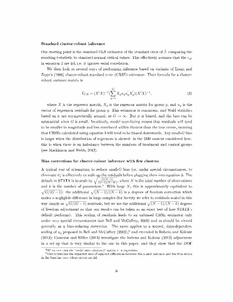
Standard cluster-robust inference
Our starting point is the standard OLS estimator of the standard error of β, comparing the
resulting t-statistic to standard normal critical values. This e�ectively assumes that the εgt
in equation 2 are iid, i.e. it ignores serial correlation.
We then look at several ways of performing inference based on variants of Liang and
Zeger's (1986) cluster-robust standard error (CRSE) estimator. Their formula for a cluster-
robust variance matrix is
VCR = (X ′X)−1(
G∑g=1
Xgugu′
gX′
g)(X′X)−1, (3)
where X is the regressor matrix, Xg is the regressor matrix for group g, and ug is the
vector of regression residuals for group g. This estimator is consistent, and Wald statistics
based on it are asymptotically normal, as G → ∞. But it is biased, and the bias can be
substantial when G is small. Intuitively, model over-�tting means that residuals will tend
to be smaller in magnitude and less correlated within clusters than the true errors, meaning
that CRSEs calculated using equation 3 will tend to be biased downwards. Any small-G bias
is larger when the distribution of regressors is skewed: in the DiD context considered here,
this is when there is an imbalance between the numbers of treatment and control groups
(see Mackinnon and Webb, 2013).
Bias corrections for cluster-robust inference with few clusters
A typical way of attempting to reduce small-G bias (or, under special circumstances, to
eliminate it) is e�ectively to scale up the residuals before plugging them into equation 3. The
default in STATA is to scale by√
G(N−1)(G−1)(N−K) , where N is the total number of observations
and k is the number of parameters.4 With large N , this is approximately equivalent to√G/(G− 1): the additional
√(N − 1)/(N − k) is a degrees of freedom correction which
makes a negligible di�erence in large samples (for brevity we refer to residuals scaled in this
way simply as√G/(G− 1) residuals, but we use the additional
√(N − 1)/(N − k) degrees
of freedom adjustment so that our results can be taken as an exact test of how STATA's
default performs). This scaling of residuals leads to an unbiased CRSE estimator only
under very special circumstances (see Bell and McCa�rey, 2002) and so should be viewed
generally as a bias-reducing correction. The same applies to a second, data-dependent
scaling of ug proposed in Bell and McCa�rey (2002),5 and extended in Imbens and Kolesár
(2012); Cameron and Miller (2013) investigate the Imbens and Kolesár (2012) adjustment
in a set-up that is very similar to the one in this paper, and they show that the DOF
4When one uses the �vce(cluster clustvar)� option in a regression.5This minimizes the expected sum of squared di�erences between the scaled residuals and the true errors
in the baseline case where errors are iid.
6
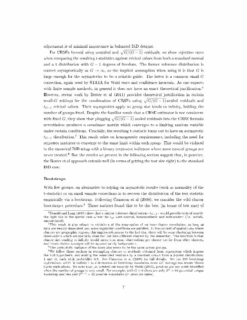
adjustment is of minimal importance in balanced DiD designs.
For CRSEs formed using unscaled and√G/(G− 1) residuals, we show rejection rates
when comparing the resulting t-statistics against critical values from both a standard normal
and a t distribution with G − 1 degrees of freedom. The former reference distribution is
correct asymptotically as G → ∞, so the implicit assumption when using it is that G is
large enough for the asymptotics to be a reliable guide. The latter is a common small-G
correction, again used by STATA for Wald tests and con�dence intervals. As one expects
with �nite sample methods, in general it does not have an exact theoretical justi�cation.6
However, recent work by Bester et al (2011) provides theoretical justi�cation in certain
small-G settings for the combination of CRSEs using√G/(G− 1)-scaled residuals and
tG−1 critical values. Their asymptotics apply as group size tends to in�nity, holding the
number of groups �xed. Despite the familiar result that a CRSE estimator is not consistent
with �xed G, they show that plugging√G/(G− 1)-scaled residuals into the CRSE formula
nevertheless produces a covariance matrix which converges to a limiting random variable
under certain conditions. Crucially, the resulting t-statistic turns out to have an asymptotic
tG−1 distribution.7 This result relies on homogeneity requirements, including the need for
regressor matrices to converge to the same limit within each group. This would be violated
in the canonical DiD setup with a binary treatment indicator where some control groups are
never treated.8 But the results we present in the following section suggest that, in practice,
the Bester et al approach extends well (in terms of getting the test size right) to the standard
DiD case.
Bootstraps
With few groups, an alternative to relying on asymptotic results (such as normality of the
t-statistic) or on small sample corrections is to recover the distribution of the test statistic
empirically via a bootstrap. Following Cameron et al (2008), we consider the wild cluster
bootstrap-t procedure.9 Those authors found this to be the best (in terms of test size) of
6Donald and Lang (2007) show that a similar reference distribution - tG−2 - would provide tests of exactlythe right size in the special case where the εgt were normal, homoscedastic and independent (i.e. seriallyuncorrelated).
7This result is also robust to violations of the assumption of no inter-cluster correlation, as long asdata are weakly dependent and some regularity conditions are satis�ed. In the context of spatial data whereclusters are geographic regions, this implies robustness to the fact that there will be some clustering betweenobservations which are spatially close but put into di�erent clusters by the researcher. The intuition is thatcluster size tending to in�nity would mean that most observations per cluster are far from other clusters,and hence cluster averages will be approximately independent.
8The asymptotic variance of the score also needs to be the same across groups.9We follow those authors in resampling clusters of residuals obtained from regressions which impose
the null hypothesis, and scaling the resampled residuals by a constant drawn from a 2-point distribution:1 and -1, each with probability 0.5. See Cameron et al (2008) for full details. We use 199 bootstrapreplications, which is su�cient in this context as bootstrap simulation error will average out across MonteCarlo replications. We note that, as pointed out recently by Webb (2013), p-values are not point identi�edwhen the number of groups is very small. For example, with G = 6 there are only 2G = 64 potential uniquebootstrap samples and 2G−1 = 32 possible t-statistics (in absolute value).
7
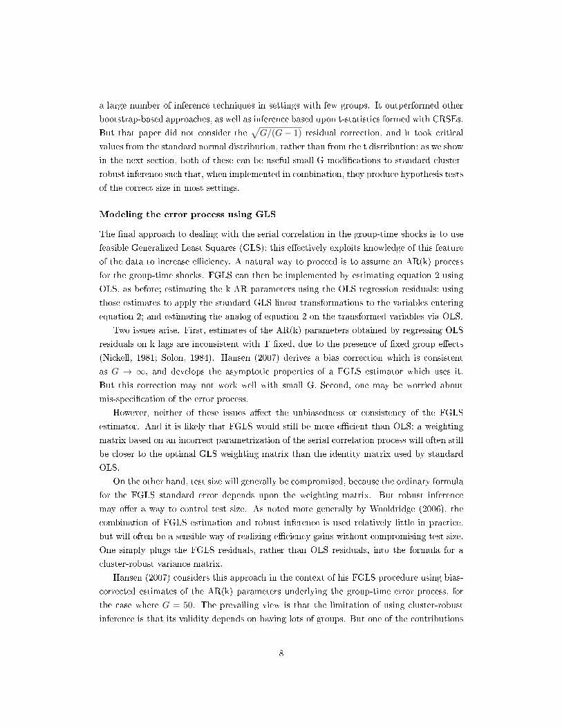
a large number of inference techniques in settings with few groups. It outperformed other
bootstrap-based approaches, as well as inference based upon t-statistics formed with CRSEs.
But that paper did not consider the√G/(G− 1) residual correction, and it took critical
values from the standard normal distribution, rather than from the t distribution; as we show
in the next section, both of these can be useful small-G modi�cations to standard cluster-
robust inference such that, when implemented in combination, they produce hypothesis tests
of the correct size in most settings.
Modeling the error process using GLS
The �nal approach to dealing with the serial correlation in the group-time shocks is to use
feasible Generalized Least Squares (GLS): this e�ectively exploits knowledge of this feature
of the data to increase e�ciency. A natural way to proceed is to assume an AR(k) process
for the group-time shocks. FGLS can then be implemented by estimating equation 2 using
OLS, as before; estimating the k AR parameters using the OLS regression residuals; using
those estimates to apply the standard GLS linear transformations to the variables entering
equation 2; and estimating the analog of equation 2 on the transformed variables via OLS.
Two issues arise. First, estimates of the AR(k) parameters obtained by regressing OLS
residuals on k lags are inconsistent with T �xed, due to the presence of �xed group e�ects
(Nickell, 1981; Solon, 1984). Hansen (2007) derives a bias correction which is consistent
as G → ∞, and develops the asymptotic properties of a FGLS estimator which uses it.
But this correction may not work well with small G. Second, one may be worried about
mis-speci�cation of the error process.
However, neither of these issues a�ect the unbiasedness or consistency of the FGLS
estimator. And it is likely that FGLS would still be more e�cient than OLS: a weighting
matrix based on an incorrect parametrization of the serial correlation process will often still
be closer to the optimal GLS weighting matrix than the identity matrix used by standard
OLS.
On the other hand, test size will generally be compromised, because the ordinary formula
for the FGLS standard error depends upon the weighting matrix. But robust inference
may o�er a way to control test size. As noted more generally by Wooldridge (2006), the
combination of FGLS estimation and robust inference is used relatively little in practice,
but will often be a sensible way of realizing e�ciency gains without compromising test size.
One simply plugs the FGLS residuals, rather than OLS residuals, into the formula for a
cluster-robust variance matrix.
Hansen (2007) considers this approach in the context of his FGLS procedure using bias-
corrected estimates of the AR(k) parameters underlying the group-time error process, for
the case where G = 50. The prevailing view is that the limitation of using cluster-robust
inference is that its validity depends on having lots of groups. But one of the contributions
8
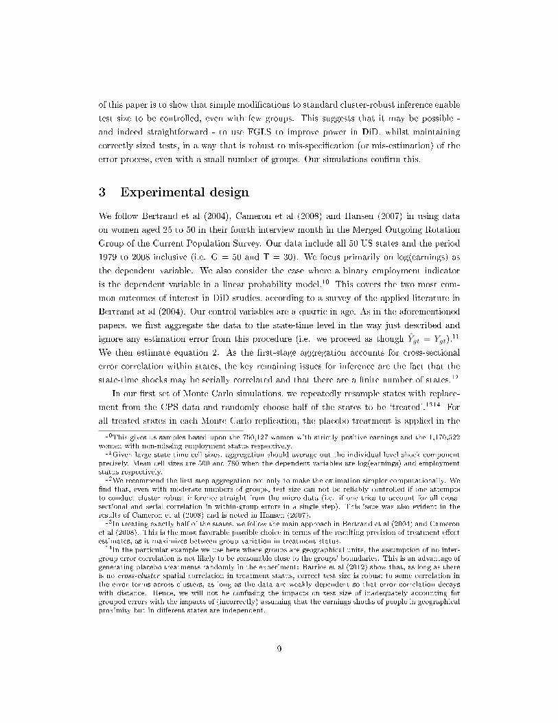
of this paper is to show that simple modi�cations to standard cluster-robust inference enable
test size to be controlled, even with few groups. This suggests that it may be possible -
and indeed straightforward - to use FGLS to improve power in DiD, whilst maintaining
correctly sized tests, in a way that is robust to mis-speci�cation (or mis-estimation) of the
error process, even with a small number of groups. Our simulations con�rm this.
3 Experimental design
We follow Bertrand et al (2004), Cameron et al (2008) and Hansen (2007) in using data
on women aged 25 to 50 in their fourth interview month in the Merged Outgoing Rotation
Group of the Current Population Survey. Our data include all 50 US states and the period
1979 to 2008 inclusive (i.e. G = 50 and T = 30). We focus primarily on log(earnings) as
the dependent variable. We also consider the case where a binary employment indicator
is the dependent variable in a linear probability model.10 This covers the two most com-
mon outcomes of interest in DiD studies, according to a survey of the applied literature in
Bertrand at al (2004). Our control variables are a quartic in age. As in the aforementioned
papers, we �rst aggregate the data to the state-time level in the way just described and
ignore any estimation error from this procedure (i.e. we proceed as though Ygt = Ygt).11
We then estimate equation 2. As the �rst-stage aggregation accounts for cross-sectional
error correlation within states, the key remaining issues for inference are the fact that the
state-time shocks may be serially correlated and that there are a �nite number of states.12
In our �rst set of Monte Carlo simulations, we repeatedly resample states with replace-
ment from the CPS data and randomly choose half of the states to be `treated'.1314 For
all treated states in each Monte Carlo replication, the placebo treatment is applied in the
10This gives us samples based upon the 750,127 women with strictly positive earnings and the 1,170,522women with non-missing employment status respectively.
11Given large state-time cell sizes, aggregation should average out the individual-level shock componentprecisely. Mean cell sizes are 500 and 780 when the dependent variables are log(earnings) and employmentstatus respectively.
12We recommend the �rst-step aggregation not only to make the estimation simpler computationally. We�nd that, even with moderate numbers of groups, test size can not be reliably controlled if one attemptsto conduct cluster-robust inference straight from the micro-data (i.e. if one tries to account for all cross-sectional and serial correlation in within-group errors in a single step). This issue was also evident in theresults of Cameron et al (2008) and is noted in Hansen (2007).
13In treating exactly half of the states, we follow the main approach in Bertrand et al (2004) and Cameronet al (2008). This is the most favorable possible choice in terms of the resulting precision of treatment e�ectestimates, as it maximizes between-group variation in treatment status.
14In the particular example we use here where groups are geographical units, the assumption of no inter-group error correlation is not likely to be reasonable close to the groups' boundaries. This is an advantage ofgenerating placebo treatments randomly in the experiment: Barrios et al (2012) show that, as long as thereis no cross-cluster spatial correlation in treatment status, correct test size is robust to some correlation inthe error terms across clusters, as long as the data are weakly dependent so that error correlation decayswith distance. Hence, we will not be confusing the impacts on test size of inadequately accounting forgrouped errors with the impacts of (incorrectly) assuming that the earnings shocks of people in geographicalproximity but in di�erent states are independent.
9
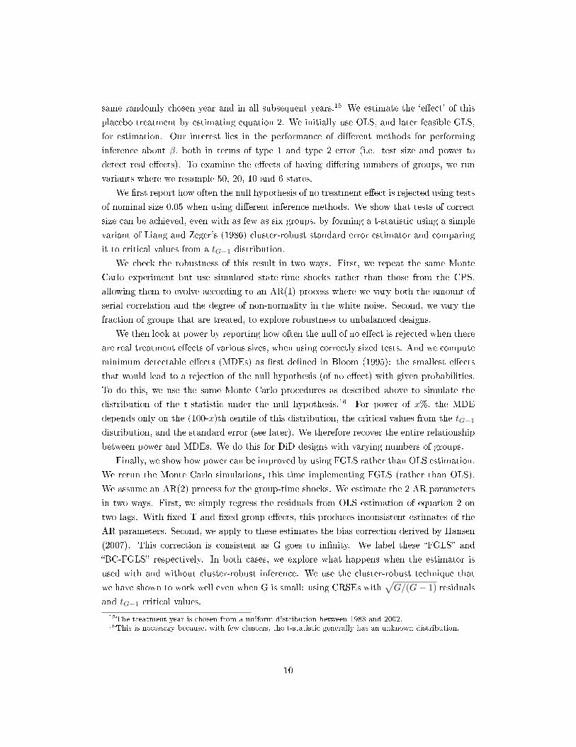
same randomly chosen year and in all subsequent years.15 We estimate the `e�ect' of this
placebo treatment by estimating equation 2. We initially use OLS, and later feasible GLS,
for estimation. Our interest lies in the performance of di�erent methods for performing
inference about β, both in terms of type 1 and type 2 error (i.e. test size and power to
detect real e�ects). To examine the e�ects of having di�ering numbers of groups, we run
variants where we resample 50, 20, 10 and 6 states.
We �rst report how often the null hypothesis of no treatment e�ect is rejected using tests
of nominal size 0.05 when using di�erent inference methods. We show that tests of correct
size can be achieved, even with as few as six groups, by forming a t-statistic using a simple
variant of Liang and Zeger's (1986) cluster-robust standard error estimator and comparing
it to critical values from a tG−1 distribution.
We check the robustness of this result in two ways. First, we repeat the same Monte
Carlo experiment but use simulated state-time shocks rather than those from the CPS,
allowing them to evolve according to an AR(1) process where we vary both the amount of
serial correlation and the degree of non-normality in the white noise. Second, we vary the
fraction of groups that are treated, to explore robustness to unbalanced designs.
We then look at power by reporting how often the null of no e�ect is rejected when there
are real treatment e�ects of various sizes, when using correctly sized tests. And we compute
minimum detectable e�ects (MDEs) as �rst de�ned in Bloom (1995): the smallest e�ects
that would lead to a rejection of the null hypothesis (of no e�ect) with given probabilities.
To do this, we use the same Monte Carlo procedures as described above to simulate the
distribution of the t-statistic under the null hypothesis.16 For power of x%, the MDE
depends only on the (100-x)th centile of this distribution, the critical values from the tG−1
distribution, and the standard error (see later). We therefore recover the entire relationship
between power and MDEs. We do this for DiD designs with varying numbers of groups.
Finally, we show how power can be improved by using FGLS rather than OLS estimation.
We rerun the Monte Carlo simulations, this time implementing FGLS (rather than OLS).
We assume an AR(2) process for the group-time shocks. We estimate the 2 AR parameters
in two ways. First, we simply regress the residuals from OLS estimation of equation 2 on
two lags. With �xed T and �xed group e�ects, this produces inconsistent estimates of the
AR parameters. Second, we apply to these estimates the bias correction derived by Hansen
(2007). This correction is consistent as G goes to in�nity. We label these �FGLS� and
�BC-FGLS� respectively. In both cases, we explore what happens when the estimator is
used with and without cluster-robust inference. We use the cluster-robust technique that
we have shown to work well even when G is small: using CRSEs with√G/(G− 1) residuals
and tG−1 critical values.
15The treatment year is chosen from a uniform distribution between 1988 and 2002.16This is necessary because, with few clusters, the t-statistic generally has an unknown distribution.
10

4 Results
4.1 Rejection rates when the null is true
Table 1 contains results from our �rst Monte Carlo simulations, using the CPS log(earnings)
data. It shows the rate with which the null of no e�ect is rejected when generating placebo
treatments, estimating equation 2 by OLS, and using methods to perform inference about β.
All hypothesis tests are of nominal size 0.05. Hence, rejection rates that deviate signi�cantly
from 0.05 indicate incorrect test size. We use 5000 replications. Simulation standard errors
are shown in parentheses. The standard error for an estimated rejection rate r is se(r) =√r(1− r)/4999.The �rst row of table 1 shows the rejection rates obtained assuming iid errors, i.e. by
simply forming a t-statistic using the OLS standard error and comparing to standard normal
critical values. Rejection rates exceed 40%, more than eight times the nominal test size.
This essentially replicates the result in Bertrand et al (2004).
Forming CRSEs using unscaled OLS residuals and comparing the resulting t-statistic to
standard normal critical values results in rejection rates that are too high, particularly with
small G. Using tG−1 rather than the standard normal as the reference distribution is enough
to achieve approximately the correct test size when G ≥ 20, but not with 6 or 10 groups.
The√G/(G− 1) residual correction, combined with tG−1 critical values, achieves a
test size that deviates by less than 1 percentage point from the nominal test size when G
ranges between 6 and 50. The same residual correction combined with standard normal
critical values also works well for moderate G but, as expected, these critical values result
in over-rejection when G is small.
The �nal row of table 1 shows rejection rates obtained using the wild cluster bootstrap-t
procedure. We essentially replicate previous �ndings: it also performs very well relative to
most tested alternatives.
In summary, table 1 suggests that tests of the correct size can be obtained using very
straightforward methods even with very few groups. In particular, this is achieved by com-
puting a t-statistic with CRSEs that use residuals scaled by√
G(N−1)(G−1)(N−K) ≈
√G/(G− 1)
, and using critical values from a t distribution with (G − 1) degrees of freedom. This is
trivial to implement with statistical software. In fact, if one uses a cluster-robust variance
matrix in STATA by specifying the �vce(cluster clustvar)� option, the con�dence intervals
and p-values returned are based upon precisely this procedure by default.17
In table 2 we present results from an analogous set of Monte Carlo simulations using
employment status rather than earnings as the dependent variable.18 The performance of
di�erent inference methods in data containing varying numbers of groups is essentially the
17This is true at the time of writing (STATA version 12.1) and has been the case since at least STATA 6.18Given that we collapse the data to the state-time level in a �rst stage, this means that Ygt now represents
state-time employment rates rather than mean state-time earnings.
11
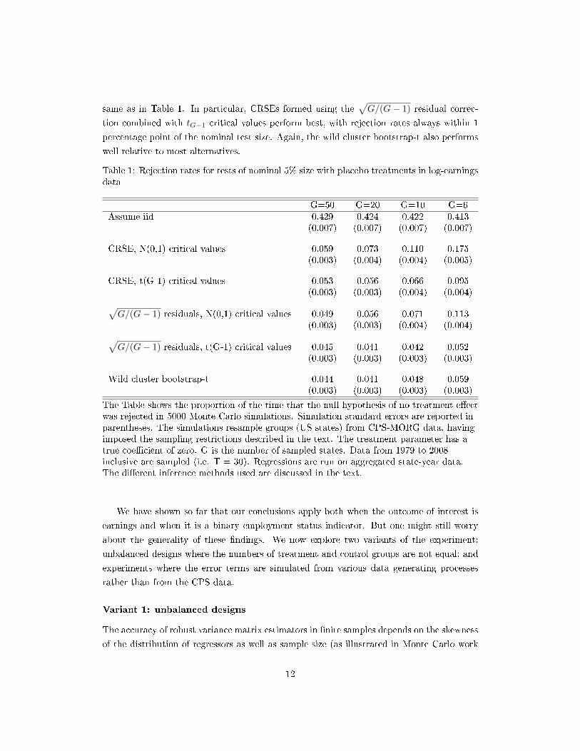
same as in Table 1. In particular, CRSEs formed using the√G/(G− 1) residual correc-
tion combined with tG−1 critical values perform best, with rejection rates always within 1
percentage point of the nominal test size. Again, the wild cluster bootstrap-t also performs
well relative to most alternatives.
Table 1: Rejection rates for tests of nominal 5% size with placebo treatments in log-earningsdata
G=50 G=20 G=10 G=6Assume iid 0.429 0.424 0.422 0.413
(0.007) (0.007) (0.007) (0.007)
CRSE, N(0,1) critical values 0.059 0.073 0.110 0.175(0.003) (0.004) (0.004) (0.005)
CRSE, t(G-1) critical values 0.053 0.056 0.066 0.095(0.003) (0.003) (0.004) (0.004)√
G/(G− 1) residuals, N(0,1) critical values 0.049 0.056 0.071 0.113(0.003) (0.003) (0.004) (0.004)√
G/(G− 1) residuals, t(G-1) critical values 0.045 0.041 0.042 0.052(0.003) (0.003) (0.003) (0.003)
Wild cluster bootstrap-t 0.044 0.041 0.048 0.059(0.003) (0.003) (0.003) (0.003)
The Table shows the proportion of the time that the null hypothesis of no treatment e�ectwas rejected in 5000 Monte Carlo simulations. Simulation standard errors are reported inparentheses. The simulations resample groups (US states) from CPS-MORG data, havingimposed the sampling restrictions described in the text. The treatment parameter has atrue coe�cient of zero. G is the number of sampled states. Data from 1979 to 2008inclusive are sampled (i.e. T = 30). Regressions are run on aggregated state-year data.The di�erent inference methods used are discussed in the text.
We have shown so far that our conclusions apply both when the outcome of interest is
earnings and when it is a binary employment status indicator. But one might still worry
about the generality of these �ndings. We now explore two variants of the experiment:
unbalanced designs where the numbers of treatment and control groups are not equal; and
experiments where the error terms are simulated from various data generating processes
rather than from the CPS data.
Variant 1: unbalanced designs
The accuracy of robust variance matrix estimators in �nite samples depends on the skewness
of the distribution of regressors as well as sample size (as illustrated in Monte Carlo work
12
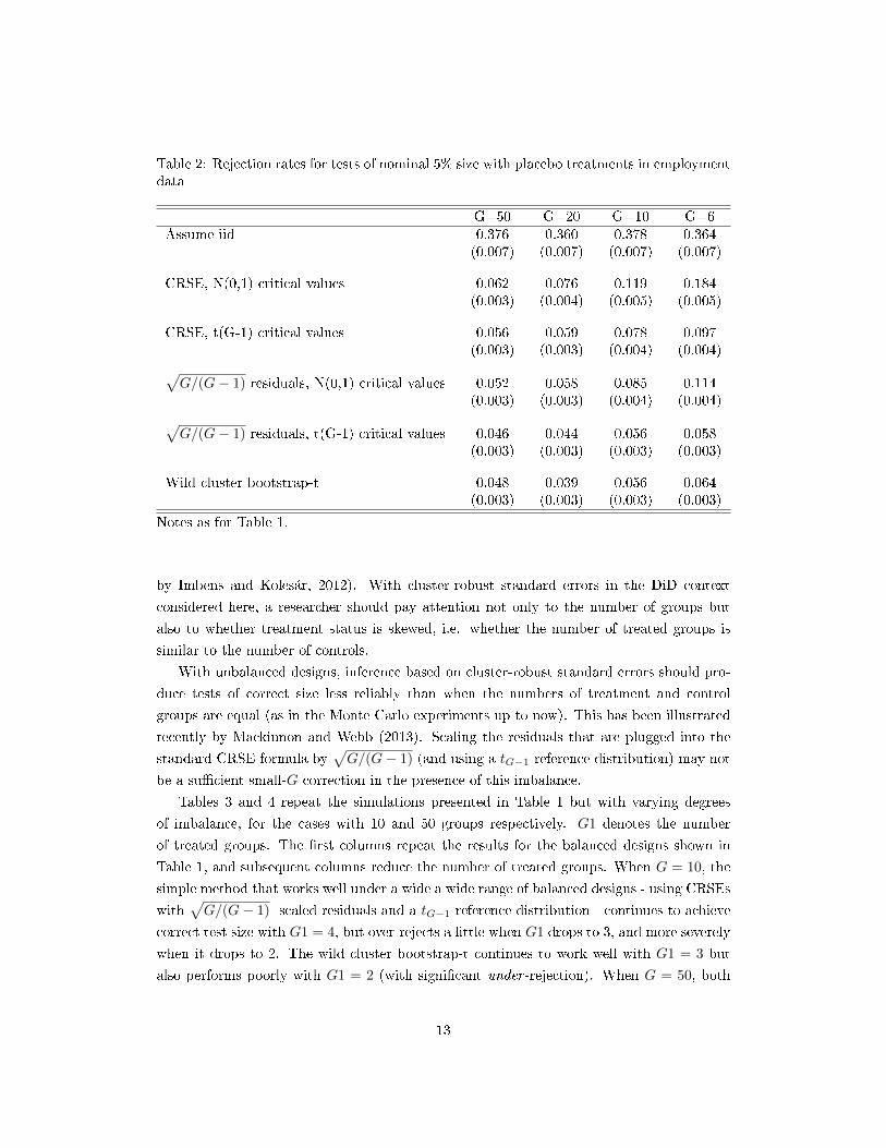
Table 2: Rejection rates for tests of nominal 5% size with placebo treatments in employmentdata
G=50 G=20 G=10 G=6Assume iid 0.376 0.360 0.378 0.364
(0.007) (0.007) (0.007) (0.007)
CRSE, N(0,1) critical values 0.062 0.076 0.119 0.184(0.003) (0.004) (0.005) (0.005)
CRSE, t(G-1) critical values 0.056 0.059 0.078 0.097(0.003) (0.003) (0.004) (0.004)√
G/(G− 1) residuals, N(0,1) critical values 0.052 0.058 0.085 0.114(0.003) (0.003) (0.004) (0.004)√
G/(G− 1) residuals, t(G-1) critical values 0.046 0.044 0.056 0.058(0.003) (0.003) (0.003) (0.003)
Wild cluster bootstrap-t 0.048 0.039 0.056 0.064(0.003) (0.003) (0.003) (0.003)
Notes as for Table 1.
by Imbens and Kolesár, 2012). With cluster-robust standard errors in the DiD context
considered here, a researcher should pay attention not only to the number of groups but
also to whether treatment status is skewed, i.e. whether the number of treated groups is
similar to the number of controls.
With unbalanced designs, inference based on cluster-robust standard errors should pro-
duce tests of correct size less reliably than when the numbers of treatment and control
groups are equal (as in the Monte Carlo experiments up to now). This has been illustrated
recently by Mackinnon and Webb (2013). Scaling the residuals that are plugged into the
standard CRSE formula by√G/(G− 1) (and using a tG−1 reference distribution) may not
be a su�cient small-G correction in the presence of this imbalance.
Tables 3 and 4 repeat the simulations presented in Table 1 but with varying degrees
of imbalance, for the cases with 10 and 50 groups respectively. G1 denotes the number
of treated groups. The �rst columns repeat the results for the balanced designs shown in
Table 1, and subsequent columns reduce the number of treated groups. When G = 10, the
simple method that works well under a wide a wide range of balanced designs - using CRSEs
with√G/(G− 1) -scaled residuals and a tG−1 reference distribution - continues to achieve
correct test size with G1 = 4, but over-rejects a little when G1 drops to 3, and more severely
when it drops to 2. The wild cluster bootstrap-t continues to work well with G1 = 3 but
also performs poorly with G1 = 2 (with signi�cant under -rejection). When G = 50, both
13
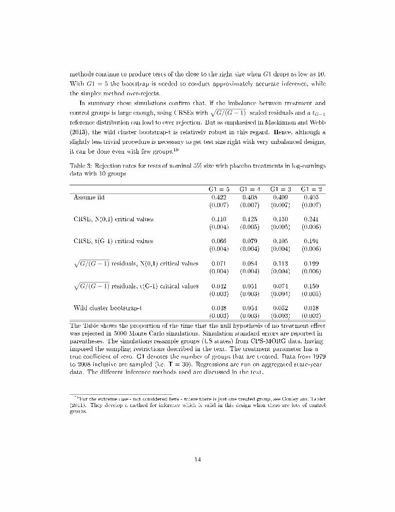
methods continue to produce tests of the close to the right size when G1 drops as low as 10.
With G1 = 5 the bootstrap is needed to conduct approximately accurate inference, while
the simpler method over-rejects.
In summary these simulations con�rm that, if the imbalance between treatment and
control groups is large enough, using CRSEs with√G/(G− 1) -scaled residuals and a tG−1
reference distribution can lead to over-rejection. But as emphasised in Mackinnon and Webb
(2013), the wild cluster bootstrap-t is relatively robust in this regard. Hence, although a
slightly less trivial procedure is necessary to get test size right with very unbalanced designs,
it can be done even with few groups.19
Table 3: Rejection rates for tests of nominal 5% size with placebo treatments in log-earningsdata with 10 groups
G1 = 5 G1 = 4 G1 = 3 G1 = 2Assume iid 0.422 0.408 0.409 0.405
(0.007) (0.007) (0.007) (0.007)
CRSE, N(0,1) critical values 0.110 0.125 0.150 0.241(0.004) (0.005) (0.005) (0.006)
CRSE, t(G-1) critical values 0.066 0.079 0.105 0.191(0.004) (0.004) (0.004) (0.006)√
G/(G− 1) residuals, N(0,1) critical values 0.071 0.084 0.113 0.199(0.004) (0.004) (0.004) (0.006)√
G/(G− 1) residuals, t(G-1) critical values 0.042 0.051 0.074 0.150(0.003) (0.003) (0.004) (0.005)
Wild cluster bootstrap-t 0.048 0.054 0.052 0.018(0.003) (0.003) (0.003) (0.002)
The Table shows the proportion of the time that the null hypothesis of no treatment e�ectwas rejected in 5000 Monte Carlo simulations. Simulation standard errors are reported inparentheses. The simulations resample groups (US states) from CPS-MORG data, havingimposed the sampling restrictions described in the text. The treatment parameter has atrue coe�cient of zero. G1 denotes the number of groups that are treated. Data from 1979to 2008 inclusive are sampled (i.e. T = 30). Regressions are run on aggregated state-yeardata. The di�erent inference methods used are discussed in the text.
19For the extreme case - not considered here - where there is just one treated group, see Conley and Tabler(2011). They develop a method for inference which is valid in this design when there are lots of controlgroups.
14
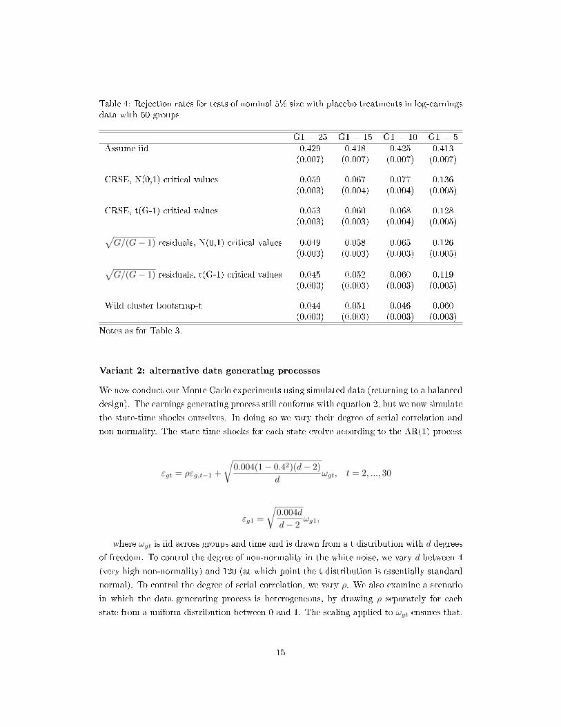
Table 4: Rejection rates for tests of nominal 5% size with placebo treatments in log-earningsdata with 50 groups
G1 = 25 G1 = 15 G1 = 10 G1 = 5Assume iid 0.429 0.418 0.425 0.413
(0.007) (0.007) (0.007) (0.007)
CRSE, N(0,1) critical values 0.059 0.067 0.077 0.136(0.003) (0.004) (0.004) (0.005)
CRSE, t(G-1) critical values 0.053 0.060 0.068 0.128(0.003) (0.003) (0.004) (0.005)√
G/(G− 1) residuals, N(0,1) critical values 0.049 0.058 0.065 0.126(0.003) (0.003) (0.003) (0.005)√
G/(G− 1) residuals, t(G-1) critical values 0.045 0.052 0.060 0.119(0.003) (0.003) (0.003) (0.005)
Wild cluster bootstrap-t 0.044 0.051 0.046 0.060(0.003) (0.003) (0.003) (0.003)
Notes as for Table 3.
Variant 2: alternative data generating processes
We now conduct our Monte Carlo experiments using simulated data (returning to a balanced
design). The earnings generating process still conforms with equation 2, but we now simulate
the state-time shocks ourselves. In doing so we vary their degree of serial correlation and
non-normality. The state-time shocks for each state evolve according to the AR(1) process
εgt = ρεg,t−1 +
√0.004(1− 0.42)(d− 2)
dωgt, t = 2, ..., 30
εg1 =
√0.004d
d− 2ωg1,
where ωgt is iid across groups and time and is drawn from a t distribution with d degrees
of freedom. To control the degree of non-normality in the white noise, we vary d between 4
(very high non-normality) and 120 (at which point the t distribution is essentially standard
normal). To control the degree of serial correlation, we vary ρ. We also examine a scenario
in which the data generating process is heterogeneous, by drawing ρ separately for each
state from a uniform distribution between 0 and 1. The scaling applied to ωgt ensures that,
15

when ρ = 0.4, the variance of εgt is equal to 0.004 - approximately the empirical variance
of the residuals in the CPS data. This means that the degree of serial correlation is allowed
to a�ect the stationary variance of εgt, but the distribution of the white noise is not. We
generate the initial condition (εg1) such that its variance matches the stationary variance
of state-time shocks in other time periods.
In each Monte Carlo replication, we �rst resample states with replacement from the CPS
data and randomly choose treated states and the year in which the placebo treatment begins,
just as before. We then regress Ygt on state and year �xed e�ects only. For each state-time
combination, we simulate the outcome variable by summing the relevant (estimated) state
e�ect, the relevant (estimated) year e�ect, and the random state-year shock generated as
above. We then estimate the DiD model using the transformed outcome and conduct the
hypothesis test on β. We use 10,000 replications.
Tables 5 to 8 report rejection rates for various combinations of ρ and d, when varying
the number of groups between 50 and 6. They show that our �nding is robust to a very
wide range of error processes. Rejection rates remain within about a percentage point of
the nominal test size under all of the tested combinations of degrees of serial correlation,
non-normality in the white noise, and number of groups.
4.2 Power to detect real e�ects
Our �ndings in the previous section indicate that controlling test size need not be a major
concern in DiD designs. However, we now show that power to detect real treatment e�ects
with tests of correct size can be extremely low.
Rejection rates in table 9 indicate power to detect treatment e�ects on earnings of
approximately 2% (precisely, 0.02 log-points), 5%, 10% and 15%. This is based upon the
same Monte Carlo replications as table 1, except we transform the dependent variable: for
example, to look at power to detect a 5% e�ect we add 0.05Tgt to Ygt.
We focus on the two methods that we have shown to produce approximately correctly
sized hypothesis tests even when the number of groups is small: the√G/(G− 1) residual
scaling combined with tG−1 critical values, and the wild cluster bootstrap-t. Nevertheless,
to ensure that we are comparing the power of hypothesis tests which have exactly the same
size, we adopt the useful procedure suggested by Davidson and Mackinnon (1998). The
nominal signi�cance level used to determine whether to reject the null hypothesis is that
which gives a test of true size 0.05. This nominal signi�cance level is obtained from the 5th
percentile of the empirical distribution of p-values from Monte Carlo simulations under a
true null (i.e. the simulations underlying the results in table 1). As the results in Table 1
suggest, for both of these methods this is a number very close (but not generally identical)
to 0.05. All results reported in Table 9 use this 'size-adjusted' measure of power.
The results indicate that power is a serious issue in these designs. A 2% e�ect would be
16
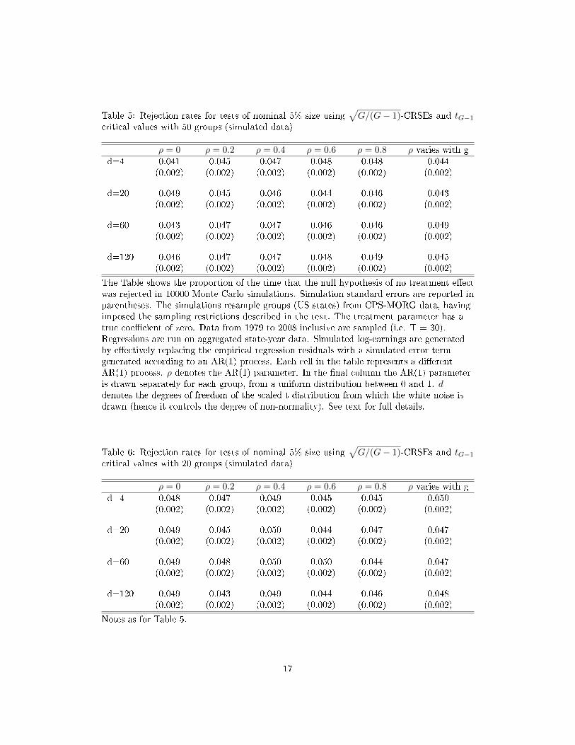
Table 5: Rejection rates for tests of nominal 5% size using√G/(G− 1)-CRSEs and tG−1
critical values with 50 groups (simulated data)
ρ = 0 ρ = 0.2 ρ = 0.4 ρ = 0.6 ρ = 0.8 ρ varies with gd=4 0.041 0.045 0.047 0.048 0.048 0.044
(0.002) (0.002) (0.002) (0.002) (0.002) (0.002)
d=20 0.049 0.045 0.046 0.044 0.046 0.043(0.002) (0.002) (0.002) (0.002) (0.002) (0.002)
d=60 0.043 0.047 0.047 0.046 0.046 0.049(0.002) (0.002) (0.002) (0.002) (0.002) (0.002)
d=120 0.046 0.047 0.047 0.048 0.049 0.045(0.002) (0.002) (0.002) (0.002) (0.002) (0.002)
The Table shows the proportion of the time that the null hypothesis of no treatment e�ectwas rejected in 10000 Monte Carlo simulations. Simulation standard errors are reported inparentheses. The simulations resample groups (US states) from CPS-MORG data, havingimposed the sampling restrictions described in the text. The treatment parameter has atrue coe�cient of zero. Data from 1979 to 2008 inclusive are sampled (i.e. T = 30).Regressions are run on aggregated state-year data. Simulated log-earnings are generatedby e�ectively replacing the empirical regression residuals with a simulated error termgenerated according to an AR(1) process. Each cell in the table represents a di�erentAR(1) process. ρ denotes the AR(1) parameter. In the �nal column the AR(1) parameteris drawn separately for each group, from a uniform distribution between 0 and 1. ddenotes the degrees of freedom of the scaled t distribution from which the white noise isdrawn (hence it controls the degree of non-normality). See text for full details.
Table 6: Rejection rates for tests of nominal 5% size using√G/(G− 1)-CRSEs and tG−1
critical values with 20 groups (simulated data)
ρ = 0 ρ = 0.2 ρ = 0.4 ρ = 0.6 ρ = 0.8 ρ varies with gd=4 0.048 0.047 0.049 0.045 0.045 0.050
(0.002) (0.002) (0.002) (0.002) (0.002) (0.002)
d=20 0.049 0.045 0.050 0.044 0.047 0.047(0.002) (0.002) (0.002) (0.002) (0.002) (0.002)
d=60 0.049 0.048 0.050 0.050 0.044 0.047(0.002) (0.002) (0.002) (0.002) (0.002) (0.002)
d=120 0.049 0.043 0.049 0.044 0.046 0.048(0.002) (0.002) (0.002) (0.002) (0.002) (0.002)
Notes as for Table 5.
17
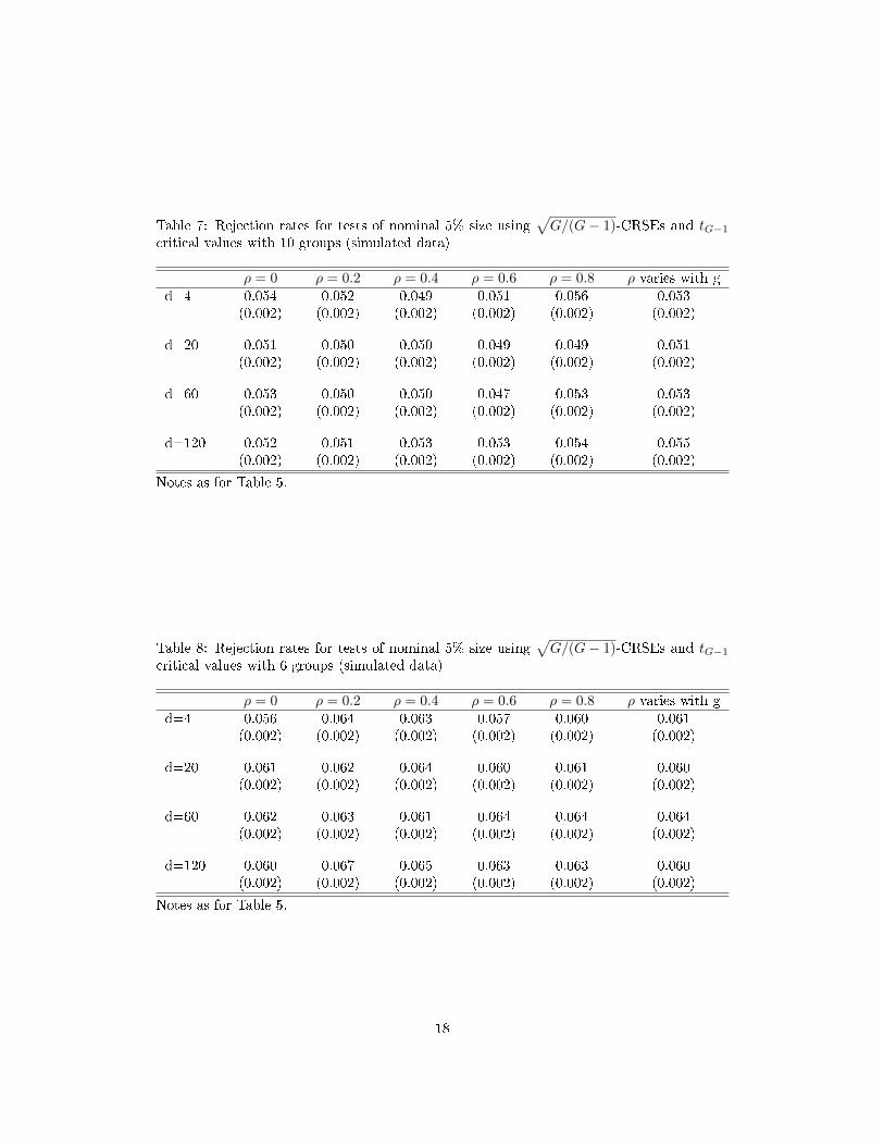
Table 7: Rejection rates for tests of nominal 5% size using√G/(G− 1)-CRSEs and tG−1
critical values with 10 groups (simulated data)
ρ = 0 ρ = 0.2 ρ = 0.4 ρ = 0.6 ρ = 0.8 ρ varies with gd=4 0.054 0.052 0.049 0.051 0.056 0.053
(0.002) (0.002) (0.002) (0.002) (0.002) (0.002)
d=20 0.051 0.050 0.050 0.049 0.049 0.051(0.002) (0.002) (0.002) (0.002) (0.002) (0.002)
d=60 0.053 0.050 0.050 0.047 0.053 0.053(0.002) (0.002) (0.002) (0.002) (0.002) (0.002)
d=120 0.052 0.051 0.053 0.053 0.054 0.055(0.002) (0.002) (0.002) (0.002) (0.002) (0.002)
Notes as for Table 5.
Table 8: Rejection rates for tests of nominal 5% size using√G/(G− 1)-CRSEs and tG−1
critical values with 6 groups (simulated data)
ρ = 0 ρ = 0.2 ρ = 0.4 ρ = 0.6 ρ = 0.8 ρ varies with gd=4 0.056 0.064 0.063 0.057 0.060 0.061
(0.002) (0.002) (0.002) (0.002) (0.002) (0.002)
d=20 0.061 0.062 0.064 0.060 0.061 0.060(0.002) (0.002) (0.002) (0.002) (0.002) (0.002)
d=60 0.062 0.063 0.061 0.064 0.064 0.064(0.002) (0.002) (0.002) (0.002) (0.002) (0.002)
d=120 0.060 0.067 0.065 0.063 0.063 0.060(0.002) (0.002) (0.002) (0.002) (0.002) (0.002)
Notes as for Table 5.
18

detected with a probability of less than 1 in 4, even with data from all 50 US states. To
detect a 5% e�ect with a probability of about 80% - a conventional benchmark for power
- one would need data on all 50 US states. Power declines much further with G. With 6
states, a researcher would have less than a 50-50 chance of detecting even a 10% e�ect, a
17% chance of detecting a 5% e�ect, and a 7% chance of detecting a 2% e�ect (power barely
greater than the size of the test). In other words, it is unlikely that one would detect e�ects
of a typically realistic magnitude using a correctly sized test, and highly unlikely when the
number of groups is small.
A comparison of the two inference methods suggests that their power is similar for
all combinations of number of groups and size of treatment e�ect. If anything, the simpler√G/(G− 1) residual scaling combined with tG−1 critical values tends to have slightly higher
size-adjusted power than the wild cluster bootstrap-t.
Figures 1 and 2 document power more comprehensively by showing the minimum e�ects
that would be detected (i.e. that would lead to a rejection of the null of no e�ect) with given
probabilities - a way of assessing statistical power �rst outlined by Bloom (1995). We vary
power between 1% and 99% and compute the minimum detectable e�ects (MDEs) in each
case. We continue just with the hypothesis test that uses CRSEs with√G/(G− 1)-scaled
residuals and tG−1 critical values.
For a given level of power, x, the MDE is
MDE(x) =ˆ
se(β)[cu − pt1−x
], (4)
whereˆ
se(β) is the√G/(G− 1)-corrected CRSE estimate, cu is the upper critical value
(the 97.5th percentile of the tG−1 distribution), and pt1−x is the (1− x)th percentile of the
t-statistic under the null hypothesis of no treatment e�ect.
We proceed with the same Monte Carlo design underlying the results in Table 1. Monte
Carlo replications provide us with an estimate of the distribution of the t-statistic under
the null. They also provide repeated estimates of the√G/(G− 1)-corrected CRSE: we
plug each of those estimates into equation 4 in turn, and take the average. Due to the low
computational intensity of this approach, we are able to use 100,000 Monte Carlo replications
so that simulation error is negligible. We use equation 4 to compute MDEs for power ranging
from 1% to 99%.
Figure 1 plots MDEs against power when the number of groups is 50, 20, 10 and 6. With
earnings data on the entire US population (50 states), one would need a treatment e�ect of
about 3.5% to have even a 50-50 chance of detecting it. With a sample from 6 US states - by
no means an extreme example in the applied DiD literature - the MDE on earnings is about
16% for 80% power and 11% for 50% power. Figure 2 shows the analagous results using a
binary employment indicator as the dependent variable. This leads to similar conclusions.
For 80% power, the MDE on the employment rate with data from all 50 states is about 2
19

Table 9: Rejection rates for tests of true 5% size with di�erent treatment e�ects (β) inlog-earnings data
G=50 G=20 G=10 G=6
β = 0.02:√G/(G− 1)-CRSEs, t(G-1) critical values 0.238 0.134 0.088 0.074
(0.006) (0.005) (0.004) (0.004)
β = 0.02: wild cluster bootstrap-t 0.225 0.125 0.093 0.074(0.006) (0.005) (0.004) (0.004)
β = 0.05:√G/(G− 1)-CRSEs, t(G-1) critical values 0.822 0.513 0.273 0.168
(0.005) (0.007) (0.006) (0.005)
β = 0.05: wild cluster bootstrap-t 0.799 0.490 0.283 0.167(0.006) (0.007) (0.006) (0.005)
β = 0.10:√G/(G− 1)-CRSEs, t(G-1) critical values 1.000 0.919 0.718 0.448
(0.000) (0.004) (0.006) (0.007)
β = 0.10: wild cluster bootstrap-t 0.999 0.898 0.712 0.429(0.000) (0.004) (0.006) (0.007)
β = 0.15:√G/(G− 1)-CRSEs, t(G-1) critical values 1.000 0.995 0.904 0.755
(.) (0.001) (0.004) (0.006)
β = 0.15: wild cluster bootstrap-t 1.000 0.992 0.896 0.700(.) (0.001) (0.004) (0.006)
The Table shows the proportion of the time that the null hypothesis of no treatment e�ectwas rejected in 5000 Monte Carlo simulations. Simulation standard errors are reported inparentheses. The simulations resample states from CPS-MORG data, having imposed thesampling restrictions described in the text. β is the true value of the treatment parameter.G is the number of sampled states. Data from 1979 to 2008 inclusive are sampled (i.e. T= 30). Regressions are run on aggregated state-year data. The inference methods used arediscussed in the text. We adjust for test size when making power comparisons using theprocedure outlined by Davidson and Mackinnon (1998). See text for details.
20
percentage points, rising to 6.5 percentage points with 6 states.20
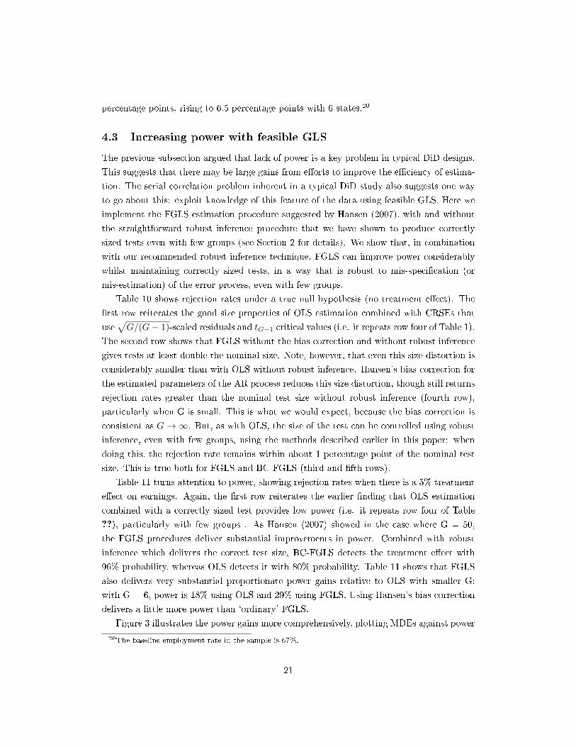
4.3 Increasing power with feasible GLS
The previous subsection argued that lack of power is a key problem in typical DiD designs.
This suggests that there may be large gains from e�orts to improve the e�ciency of estima-
tion. The serial correlation problem inherent in a typical DiD study also suggests one way
to go about this: exploit knowledge of this feature of the data using feasible GLS. Here we
implement the FGLS estimation procedure suggested by Hansen (2007), with and without
the straightforward robust inference procedure that we have shown to produce correctly
sized tests even with few groups (see Section 2 for details). We show that, in combination
with our recommended robust inference technique, FGLS can improve power considerably
whilst maintaining correctly sized tests, in a way that is robust to mis-speci�cation (or
mis-estimation) of the error process, even with few groups.
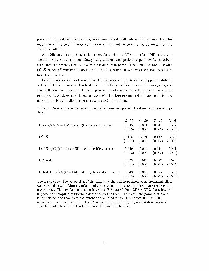
Table 10 shows rejection rates under a true null hypothesis (no treatment e�ect). The
�rst row reiterates the good size properties of OLS estimation combined with CRSEs that
use√G/(G− 1)-scaled residuals and tG−1 critical values (i.e. it repeats row four of Table 1).
The second row shows that FGLS without the bias correction and without robust inference
gives tests at least double the nominal size. Note, however, that even this size distortion is
considerably smaller than with OLS without robust inference. Hansen's bias correction for
the estimated parameters of the AR process reduces this size distortion, though still returns
rejection rates greater than the nominal test size without robust inference (fourth row),
particularly when G is small. This is what we would expect, because the bias correction is
consistent as G→∞. But, as with OLS, the size of the test can be controlled using robust
inference, even with few groups, using the methods described earlier in this paper: when
doing this, the rejection rate remains within about 1 percentage point of the nominal test
size. This is true both for FGLS and BC-FGLS (third and �fth rows).
Table 11 turns attention to power, showing rejection rates when there is a 5% treatment
e�ect on earnings. Again, the �rst row reiterates the earlier �nding that OLS estimation
combined with a correctly sized test provides low power (i.e. it repeats row four of Table
??), particularly with few groups . As Hansen (2007) showed in the case where G = 50,
the FGLS procedures deliver substantial improvements in power. Combined with robust
inference which delivers the correct test size, BC-FGLS detects the treatment e�ect with
96% probability, whereas OLS detects it with 80% probability. Table 11 shows that FGLS
also delivers very substantial proportionate power gains relative to OLS with smaller G:
with G = 6, power is 18% using OLS and 29% using FGLS. Using Hansen's bias correction
delivers a little more power than `ordinary' FGLS.
Figure 3 illustrates the power gains more comprehensively, plotting MDEs against power
20The baseline employment rate in the sample is 67%.
21

Figure 1: Minimum detectable e�ects on log-earnings using√G/(G− 1)-CRSEs and tG−1
critical values and tests of size 0.05
The Figure shows the proportion of the time that the null hypothesis of no treatmente�ect is rejected when the treatment parameter has a true coe�cient ranging from 0 to0.3. Numbers are computed using the results of 100000 Monte Carlo simulations combinedwith equation 4, as described in the text. The simulations resample states fromCPS-MORG data, having imposed the sampling restrictions described in the text. Datafrom 1979 to 2008 inclusive are sampled (i.e. T = 30). Regressions are run on aggregatedstate-year data.
22
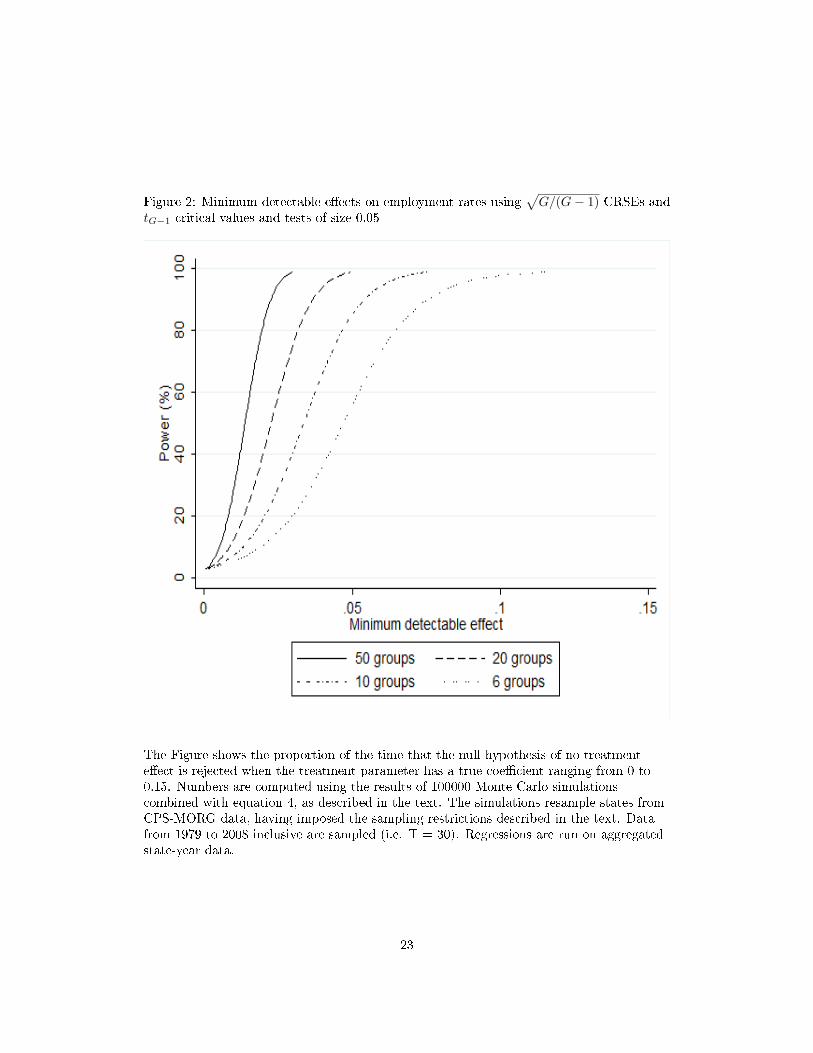
Figure 2: Minimum detectable e�ects on employment rates using√G/(G− 1)-CRSEs and
tG−1 critical values and tests of size 0.05
The Figure shows the proportion of the time that the null hypothesis of no treatmente�ect is rejected when the treatment parameter has a true coe�cient ranging from 0 to0.15. Numbers are computed using the results of 100000 Monte Carlo simulationscombined with equation 4, as described in the text. The simulations resample states fromCPS-MORG data, having imposed the sampling restrictions described in the text. Datafrom 1979 to 2008 inclusive are sampled (i.e. T = 30). Regressions are run on aggregatedstate-year data.
23

and comparing the results for OLS and BC-FGLS estimation with varying numbers of groups
(always combined with cluster-robust inference, so that test size is correct). The power gains
from BC-FGLS are substantial.
Tables 12 and 13 and Figure 4 repeat this analysis for the case where the outcome of
interest is a binary employment status indicator. This con�rms that these conclusions all
hold in that case: FGLS delivers substantial power gains over OLS, and this can be done
whilst controlling test size, even with few groups.
We now further explore the robustness of these results to di�erent data settings. Of
particular interest are cases where the parametric assumptions about the serial correlation
process inherent in the FGLS procedure are incorrect. In such cases, can test size still be
reliably controlled (even with few groups), and what power gains (if any) can FGLS o�er?
We continue to use FGLS estimation based on the assumption of an AR(2) process for
the state-time shocks which is the same for all states. We explore its properties under two
forms of mis-speci�cation of the error process. First, we simulate an AR(2) process which is
heterogeneous across states. Second, we simulate an MA(1) process with parameter 0.5.21
In each case, we e�ectively replace the empirical log-earnings residuals in the CPS (from a
regression of state-year earnings on state and year �xed e�ects) with our simulated error
terms, as in the robustness checks underlying tables 5 to 8.
Table 14 shows the results of these simulations under the null hypothesis of no treatment
e�ect using tests of nominal size 0.05, for the case where G = 10. The �rst column re-iterates
the rate at which the null hypothesis is rejected when using the empirical CPS error process
(i.e. it repeats column 3 of table 10). The next two columns report the same statistics under
the simulated error processes described above. The results show that the previous results
on test size hold under these alternative processes: without robust inference, Hansen's bias
correction for the AR parameter estimates brings true test size closer to the nominal size
when using FGLS estimation (although there is still some over-rejection); but test size can
be controlled reliably using our suggested robust inference technique, whether estimation is
carried out using OLS, FGLS or BC-FGLS.22
Table 15 reports power to detect a treatment e�ect of 0.05 log-points on earnings, again
for the case where G = 10.23 The second column shows that, using correctly sized hypothesis
21For the heterogeneous AR(2) process, the coe�cient on the �rst lag (αg1) is drawn from a uniform
distribution between zero and one for each state. The coe�cient on the second lag is set equal to 0.5 ∗min(αg
1, 1− αg1), which ensures stationarity. For both the heterogeneous AR(2) and (homogeneous) MA(1)
processes, the white noise in the process is normally distributed. Its variance is chosen so that the stationaryvariance of the simulated error term matches the empirical variance of the log-earnings residuals in the CPS(0.04).
22We showed in Section 4.1 that this inference technique is not reliable if there is a large imbalance betweenthe numbers of treatment and control groups; but that the wild cluster boostrap-t procedure is relativelyrobust in such settings. FGLS estimation combined with bootstrap-based inference would be a sensiblealternative in those situations.
23We have also conducted this analysis with G = 50. Conclusions are qualitatively the same, although ofcourse the power of all procedures is higher with more groups.
24
tests (i.e. those that use our suggested robust inference technique), FGLS estimation does
o�er substantial power gains over OLS even when based upon the incorrect assumption
that the AR(2) error process is homogeneous across states.24The third column shows that,
where the true error process is MA(1) rather than AR(2), there is no power gain from
FGLS. Intuitively this makes sense: where the parametric assumptions about the serial
correlation in the error terms are a very poor approximation to the true process, FGLS does
not o�er e�ciency gains; where the assumptions are a better approximation, FGLS does
o�er e�ciency gains over the OLS estimator, which does not exploit any knowledge of the
nature of the error process.
Finally, we show how these results vary with the number of time periods available. This is
an important dimension to explore, because we would expect the gains from modeling serial
correlation to be more signi�cant when T is large. Tables 16 and 17 repeat the simulations
with G = 10 using CPS log-earnings as the outcome variable in cases where T = 20 and
T = 10. This shows that test size can still be controlled using our recommended robust
inference approach with few time periods, whether estimation is based on OLS or FGLS. It
also shows, however, that the power gains from FGLS diminish with T, and with T = 10 the
power of OLS and FGLS (when combined with inference which provides a correctly sized
test) are essentially the same.
An interesting feature of Table 17 is that with OLS and robust inference, power actually
declines with T.25 Further inspection of the underlying simulations suggests that there is a
genuine increase in the precision of OLS estimation as T falls: the estimated policy e�ects
become more tightly distributed around their true value.
The reason why this is possible in this context is as follows.26 DiD regressions e�ectively
estimate the di�erence in mean outcomes between post-treatment periods and pre-treatment
periods (and then compare these di�erences across treatment and control groups). The
variance of this di�erence is decreasing in the covariance between the error terms pre and
post treatment (intuitively, if error terms pre and post treatment covaried perfectly then
they would not add any noise to the di�erence between pre and post treatment outcomes
because they would cancel out). If serial correlation between observations decays with time,
then the error term from an additional time period pre (post) treatment will covary less
strongly with error terms in the post (pre) treatment period than the error terms already
present. Hence the `covariance e�ect' acts to increase the variance of the DiD estimate of
the treatment e�ect when you add another time period to the data. On the other hand,
of course, the variance is also increasing in the variance of the average error terms both
24We also re-ran the earlier robustness checks where state-time earnings shocks evolve according to anAR(1) process, with varying degrees of serial correlation and varying degrees of non-normality in the whitenoise. The same qualitative conclusions about the size and power of FGLS and OLS combined with robustinference continued to hold. These results are available from the authors on request.
25The same qualitative result is reported without comment in Tables 3 to 5 of Hansen (2007).26We are extremely grateful to Joao Santos Silva for pointing out this mechanism to us.
25
pre and post treatment, and adding more time periods will reduce this variance. But this
reduction will be small if serial correlation is high, and hence it can be dominated by the
covariance e�ect.
An additional lesson, then, is that researchers who use OLS to perform DiD estimation
should be very cautious about blindly using as many time periods as possible. With serially
correlated error terms, this can result in a reduction in power. This issue does not arise with
FGLS, which e�ectively transforms the data in a way that removes the serial correlation
from the error terms.
In summary, as long as the number of time periods is not too small (approximately 10
or less), FGLS combined with robust inference is likely to o�er substantial power gains; and
even if it does not - because the error process is badly mis-speci�ed - test size can still be
reliably controlled, even with few groups. We therefore recommend this approach is used
more routinely by applied researchers doing DiD estimation.
Table 10: Rejection rates for tests of nominal 5% size with placebo treatments in log-earningsdata
G=50 G=20 G=10 G=6
OLS,√G/(G− 1)-CRSEs, t(G-1) critical values 0.045 0.041 0.042 0.052
(0.003) (0.003) (0.003) (0.003)
FGLS 0.106 0.101 0.120 0.124(0.004) (0.004) (0.005) (0.005)
FGLS,√G/(G− 1)-CRSEs, t(G-1) critical values 0.049 0.045 0.054 0.061
(0.003) (0.003) (0.003) (0.003)
BC-FGLS 0.073 0.070 0.087 0.096(0.004) (0.004) (0.004) (0.004)
BC-FGLS,√G/(G− 1)-CRSEs, t(G-1) critical values 0.049 0.045 0.058 0.065
(0.003) (0.003) (0.003) (0.003)
The Table shows the proportion of the time that the null hypothesis of no treatment e�ectwas rejected in 5000 Monte Carlo simulations. Simulation standard errors are reported inparentheses. The simulations resample groups (US states) from CPS-MORG data, havingimposed the sampling restrictions described in the text. The treatment parameter has atrue coe�cient of zero. G is the number of sampled states. Data from 1979 to 2008inclusive are sampled (i.e. T = 30). Regressions are run on aggregated state-year data.The di�erent inference methods used are discussed in the text.
26
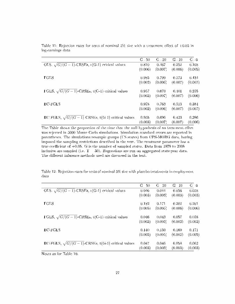
Table 11: Rejection rates for tests of nominal 5% size with a treatment e�ect of +0.05 inlog-earnings data
G=50 G=20 G=10 G=6
OLS,√G/(G− 1)-CRSEs, t(G-1) critical values 0.810 0.467 0.252 0.168
(0.006) (0.007) (0.006) (0.005)
FGLS 0.985 0.799 0.573 0.434(0.002) (0.006) (0.007) (0.007)
FGLS,√G/(G− 1)-CRSEs, t(G-1) critical values 0.957 0.670 0.401 0.255
(0.003) (0.007) (0.007) (0.006)
BC-FGLS 0.978 0.763 0.513 0.384(0.002) (0.006) (0.007) (0.007)
BC-FGLS,√G/(G− 1)-CRSEs, t(G-1) critical values 0.955 0.696 0.423 0.286
(0.003) (0.007) (0.007) (0.006)
The Table shows the proportion of the time that the null hypothesis of no treatment e�ectwas rejected in 5000 Monte Carlo simulations. Simulation standard errors are reported inparentheses. The simulations resample groups (US states) from CPS-MORG data, havingimposed the sampling restrictions described in the text. The treatment parameter has atrue coe�cient of +0.05. G is the number of sampled states. Data from 1979 to 2008inclusive are sampled (i.e. T = 30). Regressions are run on aggregated state-year data.The di�erent inference methods used are discussed in the text.
Table 12: Rejection rates for tests of nominal 5% size with placebo treatments in employmentdata
G=50 G=20 G=10 G=6
OLS,√G/(G− 1)-CRSEs, t(G-1) critical values 0.046 0.044 0.056 0.058
(0.003) (0.003) (0.003) (0.003)
FGLS 0.182 0.171 0.202 0.201(0.005) (0.005) (0.006) (0.006)
FGLS,√G/(G− 1)-CRSEs, t(G-1) critical values 0.046 0.043 0.057 0.058
(0.003) (0.003) (0.003) (0.003)
BC-FGLS 0.140 0.130 0.160 0.171(0.005) (0.005) (0.005) (0.005)
BC-FGLS,√G/(G− 1)-CRSEs, t(G-1) critical values 0.047 0.046 0.058 0.062
(0.003) (0.003) (0.003) (0.003)
Notes as for Table 10.
27
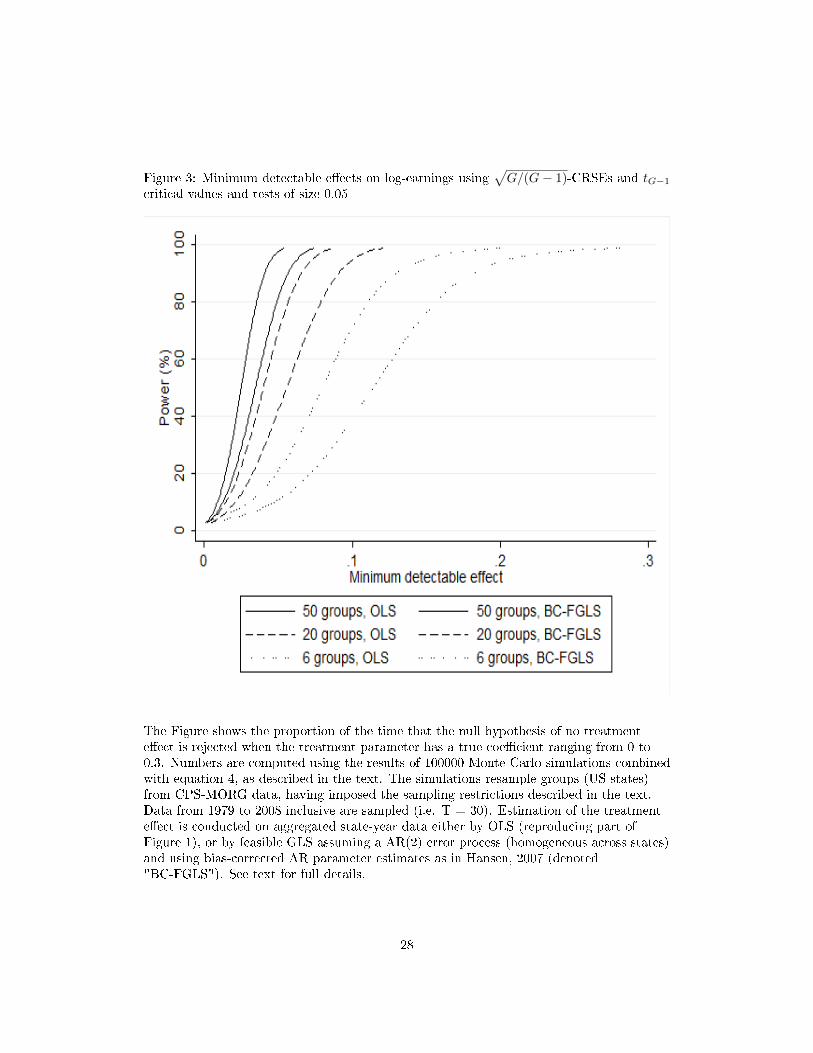
Figure 3: Minimum detectable e�ects on log-earnings using√G/(G− 1)-CRSEs and tG−1
critical values and tests of size 0.05
The Figure shows the proportion of the time that the null hypothesis of no treatmente�ect is rejected when the treatment parameter has a true coe�cient ranging from 0 to0.3. Numbers are computed using the results of 100000 Monte Carlo simulations combinedwith equation 4, as described in the text. The simulations resample groups (US states)from CPS-MORG data, having imposed the sampling restrictions described in the text.Data from 1979 to 2008 inclusive are sampled (i.e. T = 30). Estimation of the treatmente�ect is conducted on aggregated state-year data either by OLS (reproducing part ofFigure 1), or by feasible GLS assuming a AR(2) error process (homogeneous across states)and using bias-corrected AR parameter estimates as in Hansen, 2007 (denoted"BC-FGLS"). See text for full details.
28
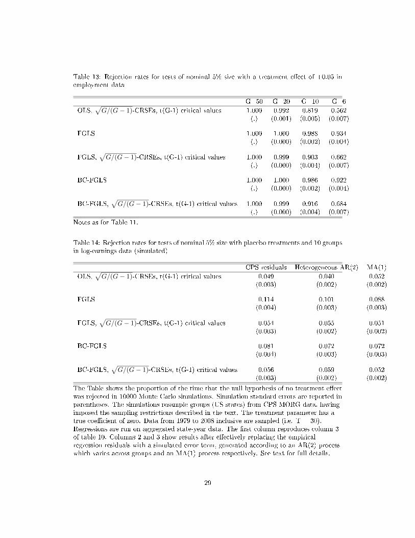
Table 13: Rejection rates for tests of nominal 5% size with a treatment e�ect of +0.05 inemployment data
G=50 G=20 G=10 G=6
OLS,√G/(G− 1)-CRSEs, t(G-1) critical values 1.000 0.992 0.819 0.562
(.) (0.001) (0.005) (0.007)
FGLS 1.000 1.000 0.988 0.934(.) (0.000) (0.002) (0.004)
FGLS,√G/(G− 1)-CRSEs, t(G-1) critical values 1.000 0.999 0.903 0.662
(.) (0.000) (0.004) (0.007)
BC-FGLS 1.000 1.000 0.986 0.922(.) (0.000) (0.002) (0.004)
BC-FGLS,√G/(G− 1)-CRSEs, t(G-1) critical values 1.000 0.999 0.916 0.684
(.) (0.000) (0.004) (0.007)
Notes as for Table 11.
Table 14: Rejection rates for tests of nominal 5% size with placebo treatments and 10 groupsin log-earnings data (simulated)
CPS residuals Heterogeneous AR(2) MA(1)
OLS,√G/(G− 1)-CRSEs, t(G-1) critical values 0.049 0.040 0.052
(0.003) (0.002) (0.002)
FGLS 0.114 0.101 0.088(0.004) (0.003) (0.003)
FGLS,√G/(G− 1)-CRSEs, t(G-1) critical values 0.054 0.055 0.051
(0.003) (0.002) (0.002)
BC-FGLS 0.081 0.072 0.072(0.004) (0.003) (0.003)
BC-FGLS,√G/(G− 1)-CRSEs, t(G-1) critical values 0.056 0.059 0.052
(0.003) (0.002) (0.002)
The Table shows the proportion of the time that the null hypothesis of no treatment e�ectwas rejected in 10000 Monte Carlo simulations. Simulation standard errors are reported inparentheses. The simulations resample groups (US states) from CPS-MORG data, havingimposed the sampling restrictions described in the text. The treatment parameter has atrue coe�cient of zero. Data from 1979 to 2008 inclusive are sampled (i.e. T = 30).Regressions are run on aggregated state-year data. The �rst column reproduces column 3of table 10. Columns 2 and 3 show results after e�ectively replacing the empiricalregression residuals with a simulated error term, generated according to an AR(2) processwhich varies across groups and an MA(1) process respectively. See text for full details.
29
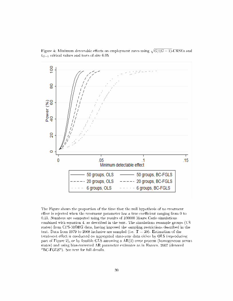
Figure 4: Minimum detectable e�ects on employment rates using√G/(G− 1)-CRSEs and
tG−1 critical values and tests of size 0.05
The Figure shows the proportion of the time that the null hypothesis of no treatmente�ect is rejected when the treatment parameter has a true coe�cient ranging from 0 to0.15. Numbers are computed using the results of 100000 Monte Carlo simulationscombined with equation 4, as described in the text. The simulations resample groups (USstates) from CPS-MORG data, having imposed the sampling restrictions described in thetext. Data from 1979 to 2008 inclusive are sampled (i.e. T = 30). Estimation of thetreatment e�ect is conducted on aggregated state-year data either by OLS (reproducingpart of Figure 2), or by feasible GLS assuming a AR(2) error process (homogeneous acrossstates) and using bias-corrected AR parameter estimates as in Hansen, 2007 (denoted"BC-FGLS"). See text for full details.
30
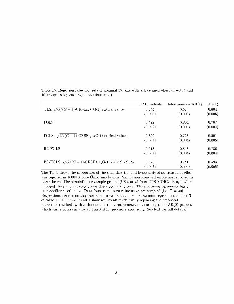
Table 15: Rejection rates for tests of nominal 5% size with a treatment e�ect of +0.05 and10 groups in log-earnings data (simulated)
CPS residuals Heterogeneous AR(2) MA(1)
OLS,√G/(G− 1)-CRSEs, t(G-1) critical values 0.254 0.510 0.604
(0.006) (0.005) (0.005)
FGLS 0.572 0.864 0.767(0.007) (0.003) (0.004)
FGLS,√G/(G− 1)-CRSEs, t(G-1) critical values 0.399 0.723 0.591
(0.007) (0.004) (0.005)
BC-FGLS 0.518 0.843 0.736(0.007) (0.004) (0.004)
BC-FGLS,√G/(G− 1)-CRSEs, t(G-1) critical values 0.423 0.741 0.593
(0.007) (0.004) (0.005)
The Table shows the proportion of the time that the null hypothesis of no treatment e�ectwas rejected in 10000 Monte Carlo simulations. Simulation standard errors are reported inparentheses. The simulations resample groups (US states) from CPS-MORG data, havingimposed the sampling restrictions described in the text. The treatment parameter has atrue coe�cient of +0.05. Data from 1979 to 2008 inclusive are sampled (i.e. T = 30).Regressions are run on aggregated state-year data. The �rst column reproduces column 3of table 11. Columns 2 and 3 show results after e�ectively replacing the empiricalregression residuals with a simulated error term, generated according to an AR(2) processwhich varies across groups and an MA(1) process respectively. See text for full details.
31
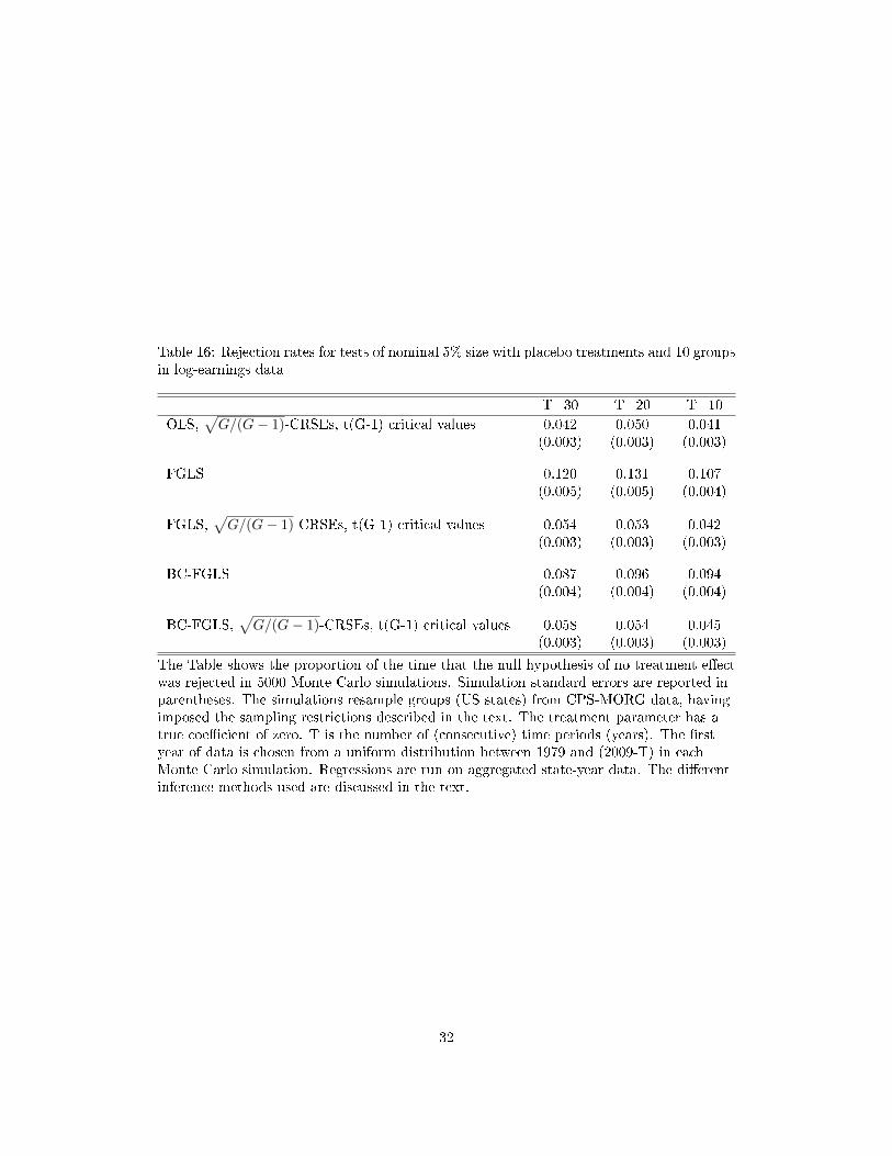
Table 16: Rejection rates for tests of nominal 5% size with placebo treatments and 10 groupsin log-earnings data
T=30 T=20 T=10
OLS,√G/(G− 1)-CRSEs, t(G-1) critical values 0.042 0.050 0.041
(0.003) (0.003) (0.003)
FGLS 0.120 0.131 0.107(0.005) (0.005) (0.004)
FGLS,√G/(G− 1)-CRSEs, t(G-1) critical values 0.054 0.053 0.042
(0.003) (0.003) (0.003)
BC-FGLS 0.087 0.096 0.094(0.004) (0.004) (0.004)
BC-FGLS,√G/(G− 1)-CRSEs, t(G-1) critical values 0.058 0.054 0.045
(0.003) (0.003) (0.003)
The Table shows the proportion of the time that the null hypothesis of no treatment e�ectwas rejected in 5000 Monte Carlo simulations. Simulation standard errors are reported inparentheses. The simulations resample groups (US states) from CPS-MORG data, havingimposed the sampling restrictions described in the text. The treatment parameter has atrue coe�cient of zero. T is the number of (consecutive) time periods (years). The �rstyear of data is chosen from a uniform distribution between 1979 and (2009-T) in eachMonte Carlo simulation. Regressions are run on aggregated state-year data. The di�erentinference methods used are discussed in the text.
32

Table 17: Rejection rates for tests of nominal 5% size with a treatment e�ect of +0.05 and10 groups in log-earnings data
T=30 T=20 T=10
OLS,√G/(G− 1)-CRSEs, t(G-1) critical values 0.252 0.274 0.310
(0.006) (0.006) (0.007)
FGLS 0.573 0.545 0.460(0.007) (0.007) (0.007)
FGLS,√G/(G− 1)-CRSEs, t(G-1) critical values 0.401 0.362 0.307
(0.007) (0.007) (0.007)
BC-FGLS 0.513 0.492 0.434(0.007) (0.007) (0.007)
BC-FGLS,√G/(G− 1)-CRSEs, t(G-1) critical values 0.423 0.388 0.316
(0.007) (0.007) (0.007)
The Table shows the proportion of the time that the null hypothesis of no treatment e�ectwas rejected in 5000 Monte Carlo simulations. Simulation standard errors are reported inparentheses. The simulations resample groups (US states) from CPS-MORG data, havingimposed the sampling restrictions described in the text. The treatment parameter has atrue coe�cient of +0.05. T is the number of (consecutive) time periods (years). The �rstyear of data is chosen from a uniform distribution between 1979 and (2009-T) in eachMonte Carlo simulation. Regressions are run on aggregated state-year data. The di�erentinference methods used are discussed in the text.
33

5 Summary and Conclusion
This paper contributes to a growing literature on inference in di�erence-in-di�erences designs
with grouped errors. The literature has emphasized di�culties in obtaining correctly sized
hypothesis tests, particularly with few groups, but our results suggest this is not the key
challenge.
Using Monte Carlo evidence, we have made three main points. First, it is possible to
obtain tests of the correct size, even with few groups, and in many settings this is possible
using methods that are very straightforward to implement. Second, the main problem
in di�erence-in-di�erences designs with grouped errors is instead low power to detect real
e�ects. Third, feasible GLS estimation combined with robust inference methods can increase
power considerably whilst maintaining correct test size - again, even with few groups. These
�ndings have proven robust to a wide range of data generating processes.
We therefore recommend that applied researchers adopt GLS estimation combined with
robust inference methods in practice. We also suggest that future research could usefully
focus on improving power, as well as on getting test size correct, when using di�erence-in-
di�erence designs.
34
References
[1] Angrist, J. and J. Pischke, Mostly Harmless Econometrics: An Empiricist's
Companion, Princeton University Press, Princeton, NJ (2009).
[2] Barrios,T. R. Diamond, G.W. Imbens and M. Kolesár, �Clustering, Spatial Cor-
relations, and Randomization Inference�, Journal of the American Statistical
Association 107:498 (2012), 578-591.
[3] Bell, R. M., and D. F. McCa�rey, �Bias Reduction in Standard Errors for
Linear Regression with Multi-Stage Samples�, Survey Methodology 28:2 (2002),
169�179.
[4] Bertrand, M., E. Du�o, and S. Mullainathan, �How Much Should We Trust
Di�erences-in-Di�erences Estimates?� Quarterly Journal of Economics 119
(2004), 249�275.
[5] Bester, A.C., T.G. Conley and C.B. Hansen, �Inference with dependent data
using cluster covariance estimators�, Journal of Econometrics 165:2 (2011),
137-151.
[6] Bloom, H. S. �Minimum Detectable E�ects: A simple way to Report the Statis-
tical Power of Experimental Designs�, Evaluation review 19:5 (1995), 547-556.
[7] Cameron, A. C., J. G. Gelbach, and D. L. Miller, �Bootstrap-Based Improve-
ments for inference with clustered errors�, The Review of Economics and Statis-
tics 90:3 (2008), 414-427.
[8] Cameron, A. C. and D. L. Miller, �A Practitioner's Guide to Cluster-Robust
Inference�, unpublished (2013).
[9] Conley, T. and C. Taber, �Inference with 'Di�erence in di�erences' with a small
number of policy changes�, The Review of Economics and Statistics 93:1 (2011),
113-125.
[10] Davidson, R. and J. G. MacKinnon, �Graphical methods for investigating the
size and power of test statistics�, The Manchester School, 66 (1998), 1-26.
[11] Donald, S. G., and K. Lang, �Inference with Di�erence-in-Di�erences and Other
Panel Data�, The Review of Economics and Statistics 89:2 (2007), 221�233.
[12] Hansen, C., �Generalized Least Squares Inference in Panel and Multilevel Mod-
els with Serial Correlation and Fixed E�ects,� Journal of Econometrics 140:2
(2007), 670-694.
35

[13] Imbens, G. and M. Kolesár, �Robust standard errors in small samples: some
practical advice�, National Bureau of Economic Research Working Paper 18478
(2012).
[14] Liang, K.-Y., and S. L. Zeger, �Longitudinal Data Analysis Using Generalized
Linear Models�, Biometrika 73 (1986), 13�22.
[15] Mackinnon, J. and Webb, M., �Wild Bootstrap Inference for Wildly Di�er-
ent Cluster Sizes�, Queen's Economics Department Working Paper No. 1314
(2013).
[16] Moulton, B. R., �An Illustration of a Pitfall in Estimating the E�ects of Ag-
gregate Variables on Micro Units�, The Review of Economics and Statistics 72
(1990), 334�338.
[17] Nickell, S., �Biases in dynamic models with �xed e�ects�, Econometrica 49:6
(1981), 1417�1426.
[18] Solon, G., �Estimating autocorrelations in �xed e�ects models�, National Bu-
reau of Economic Research Technical Working Paper 32 (1984).
[19] Webb, M., �Reworking Wild Bootstrap Based Inference for Clustered Errors�,
Queen's Economics Department Working Paper No. 1315 (2013).
[20] Wooldridge, J. M., �Cluster-Sample Methods in Applied Econometrics�, Amer-
ican Economic Review 93 (2003), 133�138.
[21] Wooldridge, J.M., �Cluster-Sample Methods in Applied Econometrics: An Ex-
tended Analysis,� mimeograph (2006), Michigan State University Department
of Economics.
36