Inequality, Hours and Labor MarketParticipation

Claudio MichelacciCEMFI and CEPR

Josep Pijoan-Mas∗

CEMFI and CEPR

October 2008Very preliminary and incomplete

Abstract

We consider a competitive equilibrium matching model where technologicalprogress is embodied in new jobs. Jobs are slowly created over time and in equilib-rium there is dispersion in job technologies. Workers can be employed in at mostone job. They decide on whether to participate in the labor market and on howmany hours to work when assigned to a job. This endogenously generates inequalityin wages and in labor supply. When the pace of technological progress acceleratesdifferences in job technologies widen. This increases wage inequality and workers de-cide to work less often but to supply longer hours once employed. The model canexplain the simultaneous fall in labor force participation and the increase in workinghours experienced by US male workers since the mid 70’s. It can also explain thedifferential effects observed across skill groups.

JEL classification: G31, J31, E24Keywords : working hours, wage inequality, human capital

∗Postal address: CEMFI, Casado del Alisal 5, 28014 Madrid, Spain. E-mail: c.michelacci@cemfi.es,pijoan@cemfi.es

1 Introduction

Some facts:

1. Since the 70’s the return to experience and other skills has increased substantially

in the US, for a review of this evidence see Gottschalk and Smeeding (1997) and

Katz and Autor (1999).

2. The fraction of prime age male workers working very long hours (say above fifty

hours per week) has increased substantially in the US over the last thirty years,

after reverting a trend of secular decline, see Costa (2000), Kuhn and Lozano (2005)

and Table 3. Average hours per male worker has also increased since the 70’s, see

McGrattan and Rogerson (2004), Figure 2 and Table 1 in the paper. The increase

has been more pronounced for relatively skilled workers, see for example Table 1 and

2 in Kuhn and Lozano (2005). Hours per worker for less than high school workers

have even fallen.

3. Kuhn and Lozano (2005) document that the increase in the fraction of workers work-

ing very long hours has been more pronounced in occupations, industries and groups

of workers (such as highly educated and high wage earners) that also experienced

higher increases in within skill wage inequality.

4. The participation rate of prime age male has declined since the 70’s, see McGrat-

tan and Rogerson (2004), Juhn (1992), and Aaronson, Fallick, Figura, Pingle, and

Wascher (2006). The decline has been more pronounced for relatively unskilled

workers, see for example Table 3 in Juhn and Potter (2006), and Table 1 and 2 in

Kuhn and Lozano (2005), Juhn (1992) and Table 1 in the paper.

5. The increase in consumption inequality has been small relative to the increase in per-

manent labor income inequality see Krueger and Perri (2006) , Heathcote, Storeslet-

ten, and Violante (2008), Heathcote, Perri, and Violante (2009), and Table 4 in the

paper.

6. There has been an acceleration in the pace of investment specific technological

progress, see Greenwood and Yorokoglu (1997), Greenwood, Hercowitz, and Krusell

(1997) and Violante (2002).

We argue that the last fact can explain the previous ones. The idea that the mid 70’s

represents a watershed for the evolution of technological progress, which caused a funda-

mental change in unemployment and wage inequality has been greatly emphasized in the

1

Figure 1: Evolution of hours and employment, descriptive statistics 34

Table 1: Fraction of Men Usually Working Long (>=50) Hours 1979 1989 2000 2006 All Men 0.161 0.193 0.190 0.178 Full Time Men (>=30 hours) 0.164 0.199 0.207 0.195 Among Full Time Men: Salaried 0.244 0.312 0.320 0.301 Hourly 0.086 0.094 0.105 0.096 Age 25-34 0.171 0.197 0.196 0.167 Age 35-44 0.185 0.221 0.222 0.208 Age 45-54 0.154 0.193 0.216 0.213 Age 55-64 0.128 0.154 0.178 0.191 Less than High School 0.124 0.121 0.116 0.099 High School Graduates 0.137 0.155 0.149 0.153 Some College 0.166 0.19 0.194 0.182 College Graduates 0.240 0.303 0.312 0.278 Average Hourly earnings quintile: 1 (highest wage) 0.151 0.243 0.297 0.268 2 0.137 0.193 0.214 0.219 3 0.132 0.176 0.199 0.189 4 0.176 0.202 0.184 0.172 5 (lowest wage) 0.217 0.186 0.151 0.133 Notes: Sample is Employed, non-self-employed, Ages 25-64.

35

Table 2: Men’s Labor Supply Indicators, by Education

1979 1989 2000 2006 AGES 25-64:

Share of Men Employed1: Less than High School 0.763 0.709 0.724 0.726 High School Graduates 0.892 0.859 0.831 0.807 Some College 0.904 0.892 0.871 0.843 College Graduates 0.940 0.928 0.914 0.890

AGES 45-54 ONLY:

Share of Men Employed1: Less than High School 0.814 0.760 0.700 0.710 High School Graduates 0.910 0.886 0.837 0.825 Some College 0.920 0.911 0.874 0.863 College Graduates 0.961 0.943 0.935 0.929

Share of Employed working Long Hours2:

Less than High School 0.111 0.126 0.111 0.110 High School Graduates 0.133 0.139 0.138 0.166 Some College 0.159 0.200 0.194 0.195 College Graduates 0.248 0.301 0.324 0.302 1. Sample: All Men 2. Sample: Men working full time (30 or more hours), not self-employed.

Notes: These are Tbale 1 and 2 from Kuhn and Lozano (2005).

literature on growth, see Greenwood and Yorokoglu (1997) and Violante (2002). This is

also consistent with the timing of changes in US aggregate data: after remaining stable for

some decades, wage inequality started to increase in the early 70s (Eckstein and Nagypal

2004) about at the same time when hours per male worker reverted a trend of secular

decline and also started to increase (McGrattan and Rogerson 2004). In accordance with

the interpretation, Kuhn and Lozano (2005)document that the increase in the number of

US workers working long hours has been more pronounced in occupations, industries and

groups of workers (such as highly educated and high wage earners) who also experienced

higher increases in wage inequality. The trend reversal in hours per worker in the US is

so far unexplained and it is a major puzzle.

We use a simple matching model in the spirit of Becker (1973) and Sattinger (1975)

that we incorporate in a standard neoclassical growth model with endogenous labor supply

to argue that these facts are the consequence of the increase in the speed of investment-

specific technical change

We emphasize the assignment friction.

As in Jovanovic (1998) we consider a competitive equilibrium matching model where

new jobs improve over time and where workers can be employed in at most one job.

Workers decide whether to participate in the labor market and once employed they decide

how many hours to work. This endogenously generates inequality in jobs, wages and labor

supply. When the pace of technological progress accelerates inequality increases, workers

decide to work less often but to supply longer hours once employed in technologically

advanced jobs. As a result labor force participation falls and hours per worker increase.

We show that this mechanism can explain several of the previously discussed unexplained

2

Figure 2: Evolution of hours and employment

41.0

42.0

43.0

44.0

45.0

46.0

1940 1950 1960 1970 1980 1990 2000

0.10

0.14

0.19

0.23

0.28

0.32

hour

s

perc

enta

geyear

Weekly Hours, US males

McGrattan - Rogerson

Kuhn - Lozano

0.60

0.70

0.80

0.90

1.00

1950 1960 1970 1980 1990 2000pe

rcen

tage

year

Employment to Population, US males

25-3435-4445-5455-64

Notes: Data from the US Census. in the left panel, the data on average hours is from McGrattan and Rogerson (2004)

and the data on fraction of males working long hours is from Kuhn and Lozano (2005). The employment rates in the right

panel comes from McGrattan and Rogerson (2004)

salient features of the evolution of male labour supply in the US since the mid seventies.

The model can also explain the differential effects by skill group.

Section 2 describes a version of the model where all workers are identical. Section

3 extends the model to allow for heterogeneity in workers skill. Section 4 evaluates

quantitatively the effects of a change in q on equilibrium labor market outcomes. Section

5 concludes. The Appendix contains the proof of some results.

2 Model with identical workers

Time is continuous and there is heterogeneity in the quality of machines available at each

point in time. We assume that every worker is matched with only one machine and a

firm can not produce with more than one worker at a time. This is the key friction of

our economy, which arises because workers and machines are indivisible. A machine of

quality k when matched with a worker who supplies e efficiency units of labor produces

an output level given by the homogenous of degree one function f(k, e)

. In this simple

version of the model we assume that e = n so that workers do not differ in skills. Workers

can supply more efficiency units of labor only by increasing their amount of hours worked.

The labor market is perfectly competitive and there are no frictions in financial markets.

The economy is populated by a mass one of potential workers and all individuals start

3

Figure 3: Evolution of hours and employment

Figure 1: Average Weekly Hours WorkedSource – The data for total hours is from Whaples (1990, Table 2.1, part A) for the period

1830-1880, Kendrick (1961, Tables A-IV and A-X) for the period for 1890–1940 and McGrattan

and Rogerson (2004, Table 1) for the period 1950-2000. The series are spliced together in 1890

and 1950. The source of data for male hours is Whaples (1990, Table 2.1, part B) for the

period 1900-1950 and McGrattan and Rogerson (2004, Table 2) for 1950–2000.

20

Notes: Average Weekly Hours Worked Source The data for all workers are from Whaples (1990, Table 2.1) for the period

1830–1880, Kendrick (1961, Table A) for the period for 1890–1940 and McGrattan and Rogerson (2004, Table 1), for

the period 1950–2000. The series are spliced together in 1890 and 1950. The source of data for male hours is Whaples

(1990, Table 2.1), for the period 1900–1950 and McGrattan and Rogerson (2004, Table 2), 2 for 1950–2000. The figure is

reproduced from Vandenbroucke (2008).

4

Table 1: Employment Population Ratio, US Census 1950-20001950 1960 1970 1980 1990 2000

All male populationTotal 0.77 0.73 0.70 0.68 0.67 0.65

By EducationLess than High School 0.77 0.67 0.61 0.51 0.45 0.43High School 0.83 0.81 0.78 0.74 0.68 0.63Some College 0.66 0.77 0.72 0.75 0.74 0.71College 0.82 0.87 0.84 0.85 0.83 0.80

Working age male population (25-65)Total 0.86 0.84 0.84 0.80 0.79 0.76

By EducationLess than High School 0.87 0.80 0.78 0.68 0.62 0.55High School 0.88 0.89 0.88 0.81 0.78 0.73Some College 0.83 0.88 0.88 0.84 0.83 0.80College 0.87 0.92 0.90 0.90 0.90 0.87

Notes: Census Data from ipums.org 1% sample. Fraction of employed workers over total population. Statistics are weighted

using individual weights. Data refers to total male population (16+), or working age male population (25-65).

5

Table 2: Population by education, US Census 1950-20001950 1960 1970 1980 1990 2000

All male population with:Less than High School 0.87 0.59 0.46 0.33 0.22 0.18High School 0.07 0.23 0.29 0.33 0.32 0.32Some College 0.03 0.09 0.13 0.17 0.26 0.27College 0.03 0.09 0.12 0.17 0.20 0.23

Working age male population (25-65) with:Less than High School 0.87 0.57 0.43 0.27 0.17 0.14High School 0.07 0.23 0.31 0.33 0.32 0.31Some College 0.03 0.09 0.11 0.18 0.27 0.28College 0.03 0.11 0.15 0.22 0.25 0.27

Notes: Census Data from ipums.org 1% sample. Distribution by educational level over total population. All quantities are

in percentage. In each panel they add up to one by column. Statistics are weighted using individual weights. Population

is either total male population (16+), or working age male population (25-65).

Table 3: Fraction of men working long hours, US Census 1980-20001980 1990 2000

All .176 .232 .288

By education:Less than High School .136 .158 .201High School .162 .193 .238Some College .184 .234 .281College .228 .310 .372

By wage quintiles:1st .130 .140 .1632nd .148 .186 .2163rd .154 .221 .2734th .178 .241 .3285th .264 .357 .451

Notes: Census Data from ipums.org 1% sample. Fraction of men usually working long hours (more than 50 hours per week)

Source: US Census 1% sample. Sample is fulltime employed men, non-self-employed, ages 25-64.

6

Table 4: Income and consumption, US CEX 1980-20001980 1990 2000

ConsumptionLess than High School 0.58 0.54 0.49High School 0.71 0.67 0.65Some College 0.82 0.78 0.75

Consumption of non Durables PlusLess than High School 0.61 0.56 0.47High School 0.73 0.68 0.64Some College 0.82 0.79 0.74

Consumption of non DurablesLess than High School 0.68 0.62 0.54High School 0.76 0.72 0.68Some College 0.84 0.81 0.77

Labor IncomeLess than High School 0.54 0.45 0.36High School 0.70 0.61 0.54Some College 0.77 0.71 0.63

Labor Income of Household HeadLess than High School 0.52 0.43 0.35High School 0.68 0.59 0.51Some College 0.75 0.68 0.61

Hourly wage of full time workersLess than High School 0.62 0.54 0.42High School 0.75 0.65 0.55Some College 0.80 0.73 0.66

Relative Consumption and relative Income. Notes: Data come from Consumer Expenditure Survey. A unit is a

household. Households are classified by the educational level of the household head. Consumption and Income are always

relative to college graduates ”Consumption” is annual total average expenditures. ”Non Durable Consumption Plus” is total

expenditures in non durable consumption goods plus expenditures in services from vehicles, housing, renting, equipment

and entertainment. ”Non Durable Consumption” is total expenditures in non durable consumption goods. ”Labor income”

is the sum of wage and salaries plus two thirds of self-employment household income; ”Labor income of Household Head”

is total labor income of household head. ”Hourly wage of full time workers” is labor income divided by annual hours

(calculated as the product of hours worked per week and weeks worked in the year) for workers who work at least 35 hours

a week and at least 40 weeks a year, as in Eckstein and Nagypal (2004) See Krueger and Perri (2006) for further details

about the CEX data set.

7

with the same amount of wealth.

2.1 Machine types

At every instant in time t, m new machines of quality eqt become available. Machines are

in excess supply because the number of workers is fixed and some new machines become

continuously available. This means that there is a critical age τ ∗ such that all machines

older than τ ∗ are scrapped. The distribution of ages is uniform on the support τ ∈ [0, τ ∗].

Let p denote the participation rate, i.e. the fraction of workers that participate to the

labour market. Since every worker is paired to a machine, p is also the amount of machines

operated in equilibrium.1 Hence, the density of machines of any age is given by mp

and

the fraction of machines in operation with age smaller than or equal to τ is given by,

Pr (τ ≤ τ) =

∫ τ

0

m

pds =

m

pτ

By definition, no machine older than τ ∗ is in operation. Clearly τ ∗ solves Pr (τ ≤ τ ∗) = 1,

which immediately implies that

τ ∗ =p

m.

It is easy to map machine ages into machine qualities. Machines depreciate at rate δ.

Then, the quality kτt of a machine of age τ at time t is given by eq(t−τ)e−δτ . Hence, the

quality k∗t of the worst machine in operation at time t can be expressed as

k∗t = eq(t−τ∗)e−δτ

∗(1)

and the ratio between the best and the worst machine in operation is given by e(q+δ) pm .

We can define the detrended machine quality as,

kτ ≡ kτt e−qt = e−(q+δ)τ

such that k∗ = e−(q+δ) pm and if we call k0 the detrended quality of the best machine, we

have k0 = 1.

Lemma 1 The distribution of detrended qualities of operating machines has support [e−(q+δ) pm , 1]

and it is log-uniform with density g (k) = m(q+δ)p

1k.

1For simplicity, we discuss the model with a constant participation rate p. This does not constraintthe solution of the model as we are going to focus on the balanced growth path equilibrium, in whichaggregate variables grow at a constant rate and aggregate ratios are constant over time. See Section 2.6for an exact definition.

8

2.2 Firms

At any point in time t, a firm with a machine of quality kt is paired with a worker and

chooses the optimal demand of efficiency units of labor nt by solving:

πt(kt) = maxnt

{f(kt, nt

)− wt(nt)

}where πt(kt) denotes firm profits and wt(nt) is the compensation for a worker that supplies

nt units of labor. The first order condition is given by

f2

(kt, nt

)= w′t (nt) (2)

This optimality condition defines a labor demand function,

nt = φt

(kt

)which establishes that the amount of hours worked in every machine type depends on

the production function and the wage function. As part of the competitive allocation

it should be that workers who are matched with better machines supply more efficiency

units of labor. This is an optimal allocation condition that arises in the competitive

equilibrium because capital and efficiency units of labor are complementary in production

and allocations are efficient,–i.e. the first welfare theorem holds. This implies that n∗t =

φt

(k∗t

)is the minimum amount of efficiency units of labor supplied in the market

Recall that machines are in excess supply and that there is a critical level of capital

quality k∗t such that all machines of smaller quality are scrapped. Free entry must yield

zero profits to operating this machine and hence the wage paid to the worker in the worst

machine must satisfy:

wt (n∗t ) = f(k∗t , n

∗t

)= f

(k∗t , φt

(k∗t

))(3)

where n∗t are the efficiency units of labor supplied by a worker matched to the worst

machine in operation. For simplicity we assume that wt (n) is equal to zero for any

n < n∗t .

2.3 Matching

The equilibrium of the economy determines how workers and machines are matched to-

gether. No party should have incentive to deviate from the equilibrium matching and

9

market should clear. To model the matching process we define two objects. Let pt,i

denote the time t probability that worker i participates in the labor market. Of course:∫[0,1]

pt,idi = p (4)

Also let ϕt,i (k) denote the probability that, conditional on participating in the labor

market, worker i is matched with a machine of de-trended quality smaller than or equal

to k. Clearly ϕt,i is zero for any k < k∗ and it has to satisfy the condition that all machines

of quality k ≥ k∗ are in use, which implies that∫[0,1]

pt,i ϕt,i (k) di = p

∫ k

k∗g (s) ds ∀k ≥ k∗ (5)

where g (s) is the density function of machine qualities described in Lemma 1. The right

hand side of equation (5) gives the number of (non-scrapped) machines of quality equal

to or less than k. The left hand side gives the expected number of workers assigned

to machines of type equal to or less than k. Since there is a continuum of workers the

expectation is equal to the average.

We model the matching process as stochastic. But, since workers are infinitely lived

and there are no borrowing constraints, this is without loss of generality due to a law of

large numbers.

2.4 Workers

Individuals are infinitely lived, with instantaneous utility given by

u (ct,i, nt,i) =c1−σt,i − 1

1− σ− v(νtnt,i)

where v(νtnt,i) is the disutility of working nt,i hours. Following Mincer (1962) and Becker

(1965) we assume that leisure is valuable to individuals because they can use their time

to produce leisure goods. In addition to time, the production of leisure goods requires

another input that can be purchased in the market. There is evidence that the decline

in the price these market goods is an important determinant of male labour supply, see

Gonzales–Chapela (2007). We assume that due to the fall the price of market goods the

utility cost of supplying hours in the market increases at rate µ, i.e. νt ≡ eµt. We assume

10

that

v (s) =

{λ0 + λ1

s1+η

1+ηif s > 0

0 if s = 0(6)

where λ0 ∈ [0, 1) is a fixed cost of going to work while λ1 > 0 is a variable component.

The parameter η regulates the Frisch elasticity.

Individuals maximize the present discounted value of their utility:

maxct,i,nt,i,pt,i

∫ ∞0

e−ρtu (ct,i, nt,i) dt

where ρ is the subjective time discount rate, subject to the sequence of budget constraints:

˙bt,i = wt,i (nt,i)− ct,i + rbt,i (7)

where bt,i are assets and wt (nt,i) denotes labour income when supplying nt,i working hours

in the market. When the worker is not participating in the labor market nt,i and wt (nt,i)

are both equal to zero. All workers start with wealth, b0, and they can choose how much

to consume and save every period as well as how many hours of work they supply in the

market. There are no liquidity constraints and the consumption good is the numeraire.

By solving the worker’s problem we obtain the standard Euler equation for the con-

sumption path,˙ct,ict,i

=1

σ(r − ρ) (8)

where ˙ct,i denotes the time derivatives and the intratemporal condition for labor supply,

v′ (νtnt,i) νt = (ct,i)−σ w′t (nt,i) . (9)

Moreover it has to be the case that

(ct,i)−σ wt (nt,i) ≥ v (νtnt,i) , (10)

for workers to choose pt,i > 0. Whenever the inequality is strict pt,i = 1, and whenever it

holds as equality the worker is indifferent at time t about the participation probability.

11

2.5 Financial markets

Firms are owned by workers. In particular, workers own shares st,i of the diversified

portfolio of firms, which entails the payment of aggregate firm profits,

Πt = p

∫ 1

k∗π(eqts)g (s) ds

Let pt denote the price of equity shares at time t. The amount of wealth bt,i of worker i

at time t is given by,

bt,i = ptst,i

Since there are no borrowing constraints in place st,i can be negative, that is, short selling

is allowed. Of course, in equilibrium ∫[0,1]

bt,idi = pt (11)

Since all workers start up with the same financial wealth b0 it means they all start with

the same share of firm ownership s0. The interest rate in the budget constraint (7) is

given by the dividend flow and the capital gains,

rt =˙ptpt

+Πt

pt(12)

2.6 Balanced growth path equilibrium

We now analyze the problem under the simplifying assumptions that σ = 1 and the

production function is Cobb-Douglas, f (k, n) = kαn1−α. We focus the analysis on the

balanced growth path equilibrium. All time periods are identical and we shall see that

in steady state output, consumption, assets and the price of equity shares grow at the

constant rate x = α(q+µ)−µ, hours decline at rate µ, the participation rate p is constant

and the interest rate is given by the modified golden rule, r = ρ+σx. The Cobb-Douglas

production function helps in guaranteeing that a steady state exists, σ = 1 implies that

the participation rate is constant in equilibrium. To characterize the steady state we

consider the de-trended variables n ≡ νtnt = eµtnt, c ≡ e−xtct, b ≡ e−xtbt and p ≡ e−xtpt,

and the de-trended functions w (n) ≡ e−xtwt (nt) and φ (k) ≡ eµtφt

(kt

).

Definition 1 A balanced growth path equilibrium for this economy is characterized by a

price of equity shares p, a wage function w (n), individual participation probabilities pt,i,

12

assignment functions ϕt,i (k), an aggregate participation rate p, an interest rate r and

individual consumption, saving and working plans and firm labor demands φ (k) such that

(a) Workers solve their optimization problem, that is, equations (7), (8), (9), and (10)

are satisfied.

(b) Firms solve their optimization problem, that is, equation (2) is satisfied,

(c) The free entry condition (3) in production is satisfied,

(d) The labor market clears, that is, equations (4) and (5) hold.

(e) The capital market clears, that is, equation (11) holds

(f) The goods market clears, that is, aggregate output is equal to aggregate consumption,

(g) Aggregate consumption and output grow at the same constant rate and the aggregate

participation rate is constant.

Notice that to characterize the balanced growth path equilibrium we need to charac-

terize simultaneously the wage function and the assignment function. We conjecture the

following wage function,

w (n) =

{a0 + a1

n1+η

1+ηif n > 0

0 if n = 0(13)

and an assignment such that workers are allocated to different machines during their

working life with the constraint that all workers obtain the same permanent income. In

equilibrium workers matched with better machines should work longer hours. Since all

workers are identical, this can be sustained in equilibrium only if workers obtain the same

permanent income. To understand why this has to be the case, argue by contradiction

and consider an assignment that puts worker i more often than worker j to work with

a good machine. Then worker i will have greater labor income and greater consumption

that will disincentive the supply of hours of worker i relative to worker j through the

income effect. But then the firm that hires worker i would make greater profits by hiring

worker j instead, because he would be willing to supply the same amount of hours as

worker i would do but at a cheaper price. As we will see below, the conjectured wage

function makes workers indifferent about how many hours to work at any given point in

time and hence workers matched to better machines are ready to supply more hours of

work. There are many different assignments that can satisfy our conjecture. Without loss

of generality, we will focus on symmetric equilibria.

13

Definition 2 A symmetric balanced growth path equilibrium is a balanced growth path

equilibrium in which,

(a) The participation probability pt,i of a worker is the same and equal to the aggregate

participation rate of the economy p,

(b) The assignment function is the same for all individuals

Note that if the participation probabilities and the assignment functions have to be

the same for all workers, then equations (4) and (5) imply

pt,i = p and ϕt,i (k) = ϕt (k) =

∫ k

k∗g (s) ds ∀k ≥ k∗

which makes clear that the participation probabilities and the assignment functions are

independent of time.

Now, given this conjecture, finding the equilibrium requires characterizing a0 and a1.

In the next sub-sections we are going to look for two equations that together pin down

their value.

2.7 The IE equation

We start by looking at the worker’s problem. The Euler equation (8) and the balanced

growth path condition determine the interest rate as the modified golden rule,

r = ρ+ x (14)

Integrating the Euler equation (8) and using (14) gives us the consumption path:

ct,i = c0,iext ⇒ ct = c0 (15)

To determine the value of c0 we integrate forward the period budget constraints (7) to

obtain, ∫ ∞0

e−rττ cτ,idτ = b0 +

∫ ∞0

e−rτ wτ (nτ,i) dτ.

Note that the the labor income wτ (nτ,i) at any period of time is stochastic as it depends

on the assignment. However, given a law of large numbers the present value of labor

14

income is equal to the cross-sectional average of labor income, which is not stochastic.2

Given (15) and (14), the previous expression simplifies to

c0,i = ρ

[b0 +

∫ ∞0

e−ρτw (nτ,i) dτ

]= ρb0 + pi

∫ k∗i−1

k∗i

w (φ (s)) dϕi (s) (16)

which is the standard permanent income condition that determines consumption c0.

Now, we can replace the disutility of work (6), the wage function (13) and the optimal

consumption path (15) into the condition for optimal labor supply (9) to obtain,

λ1 =a1

c0,i

(17)

This equation tells that, at any given point in time, all workers are indifferent about the

amount of hours they work because the value of an extra unit of time spent in leisure

and the value of an extra unit of time of work grow at the same rate as the amount of

working time increases. When paired to a good machine a worker experiences a high

utility cost of giving up scarce time for leisure, but he is paid accordingly to compensate

for these extra hours. Hence, work effort in a given period is undetermined as in Prescott,

Rogerson, and Wallenius (2006). However, this does not mean that lifetime work effort

is undetermined: given a market price a1, equation (17) determines c0,i and this puts a

constraint in lifetime work effort through the permanent income (see equation 17). Notice

also that this condition is identical for all individuals, which implies that all individuals

consume the same amount, c0,i = c0.

We focus the analysis on the case where the participation rate is positive but strictly

less than one, p ∈ (0, 1). This implies that (10) holds as an equality, which after using

(13) and (17), yields

λ0 =a0

c0

(18)

which says that the fixed utility cost of entering the labour market is equal to the utility

gain of participating to the labour market and supplying zero units of labour. Again,

at any given point in time the worker is indifferent between going to work or not. By

2To see this note that the present value of labor income can be written as∫ ∞0

e−rτ wτ (nτ,i) dτ =∫ ∞

0

e−rt

(pi

∫ k∗i−1

k∗i

extw (φ (s)) dϕi (s)

)dt =

pir − x

∫ k∗i−1

k∗i

w (φ (s)) dϕi (s)

15

combining (17) with (18) we obtain that

a0 =λ0

λ1

a1 (IE)

This equation says that a0 and a1 should be such that workers be indifferent between

how many hours they work and on whether participating or not in the labour market.

This implies that a0 and a1 should always move in the same direction. This relation

characterizes the relation between labour supply along in the intensive and extensive

margin. We call this the (IE) relationship.

2.8 The equilibrium participation rate

In order to obtain the participation rate as a function of the equilibrium wage parameters

we will use equation (17) and the market clearing condition for the goods markets. We

can obtain Y , the de-trended aggregate output, by adding the output in all machines.

Let’s first obtain the demand of labor for each machine. Substituting the conjectured

wage schedule into the optimality condition for firms (2) we obtain:(ktnt

)α

=a1

1− αe(x+µ)tnηt

After rearranging, this gives the following labor demand function in terms of detrended

quantities:

n = φ (k) =

(1− αa1

kα) 1

α+η

, (19)

which is independent of time.3 Now, aggregate output is given by,

Y = p

∫ 1

k∗

(1− αa1

) 1−αα+η

sα(1+η)α+η g (s) ds =

m

q + δ

(1− αa1

) 1−αα+η (α + η)

α (1 + η)

[1− e−

α(1+η)(q+δ)p(α+η)m

](20)

where g (s) is the density function of detrended machine qualities, see Lemma 1. In equi-

librium aggregate output should be equal to aggregate consumption. Since all individuals

consume the same this implies that c0 = Y .4 By using (20) to replace Y in (17) we

3Notice that in terms of absolute quantities the labor demand function is given by:

nt = φt

(k)

= e−µtφ(ke−qt

)4see the Appendix for a derivation from first principles

16

immediately obtain

m

q + δa− 1+ηα+η

1

[1− e−

α(1+η)(q+δ)p(α+η)m

]=

α (1 + η)

λ1 (1− α)1−αα+η (α + η)

(21)

Lemma 2 The value of p that solves (21) can be expressed as a function p = p(a1; q)

which is increasing in both a1 and q.

Equation (21) is obtained by the condition that aggregate output is equal to aggregate

consumption and that workers are indifferent about how many hours of work they supply

at any given period—both along the intensive and the extensive margin. The right hand

side in (21) is decreasing in a1 because with a rise in a1 every hour hired by a firm is

more expensive and firms reduce their demand for labour. The right hand side in (21) is

increasing in p because an increase in the amount of machines used increases overall output

and consumption. To better understand the logic of the dependence between a1 and p

notice that an increase in a1 reduces aggregate output and aggregate consumption because

firms rent less labour. As a result the right hand of (18) increases more workers would like

to participate in the labour market. This makes p increases which pushes consumption

up to the point where the equality (18) is restored. The right hand side is decreasing

in q because a larger q implies a larger spread of machine qualities in equilibrium and

a lower mass of machines operating the leading technology. This reduces labor demand

and detrended consumption. To restore the equality (18), then p should increases. The

function p(a1; q) determines the participation rate in the economy provided that it is a

quantity in the unit interval. If it is greater than one all workers participate and p = 1.

2.9 The FE equation

Then, the free entry condition (3) determines the wage paid at the worst machine. Taking

the wage function (13) we can write,

a0 + a1(n∗)1+η

1 + η= e−α(q+δ)τ∗ (n∗)1−α (22)

where, using equation (19), n∗ is given by:

n∗ =

(1− α

a1eα(q+δ)τ∗

) 1α+η

(23)

17

which substituted into the above expression and after rearranging yields5

a0 =(1− α)

1−αα+η (α + η)

1 + ηe−

(1+η)α(q+δ)p(a1;q)(α+η)m (a1)−

(1−α)α+η (FE)

where the function p is defined in Lemma 2. The (FE) condition determines a negatively

sloped relationship between a0 and a1. There are two reasons for this. First, an increase

in a1 lowers the profits per machine and hence the rents captured by workers through

a0 decline. Second, an increase in a1 increases the equilibrium participation rate p (see

Lemma 2). This implies that more and worse machines are used in equilibrium and hence

the income generated by the worst machines is lower and so are the rents captured by

workers through a0.

2.10 The equilibrium allocations

The equations (IE) and (FE) determine the unique pair a0 and a1 consistent with the

equilibrium. This equilibrium determination can be easily analyzed by plotting the corre-

sponding graphs in the a0 and a1 space, see Figure 4. After determining a1, p is determined

using (21) while the average amount of detrended hours per worker is given by

n =1

p

∫ 1

e−qpm

φ (s) g (s) ds =

(α + η

α

)(1− αa1

) 1α+η m

qp

[1− e−

αqp(α+η)m

]. (24)

Observed average hours per worker are instead given by e−µtn.

2.11 The effects of an increase in q

There is much evidence that the pace of investment specific technological progress has

speeded up, see Greenwood and Yorokoglu (1997), Greenwood, Hercowitz, and Krusell

(1997) and Violante (2002). In our model this corresponds to an increase in q. We now

analyze the effects of an increase in q.

5To see this notice that

a0 + (a1)−(1−α)α+η

(e−α(q+δ)τ∗

) 1+ηα+η (1− α)

1−αα+η+1

1 + η=

(e−α(q+δ)τ∗

) 1+ηα+η

(a1)−(1−α)α+η (1− α)

1−αα+η

a0 =(1− α)

1−αα+η (α+ η)

1 + η

(e−α(q+δ)τ∗

) 1+ηα+η

(1a1

) 1−αα+η

a0 =(1− α)

1−αα+η (α+ η)

1 + η

(e−α(q+δ)τ∗ 1

a1

) 1+ηα+η

18

Figure 4: Equilibrium determination of a0 and a1

IE

FE

a1

a0

IE

FE

a1

a0

Dq

Lemma 3 When q increases both a0 and a1 fall.

The intuition for this result is as follows. Holding a1 constant, an increase in q makes

a0 to fall in order to satisfy the free entry condition (FE). The increase in q has two effects.

First, as shown in Lemma 2, it increases p. This implies that more and worse machines are

operated in equilibrium and hence the income generated by the marginal machine is lower

and hence so is the a0 that gives zero profits. Second, holding p constant, the increase

in q also reduces the quality of the worst machine relative to trend. This further reduces

the income generated at the marginal machine and hence a0. This implies a downward

shift of (FE). Since the relationship (IE) is invariant to q and positively sloped, a1 will

also fall in equilibrium.

Lemma 4 When q increases the quality gap e(q+δ) pm between the best and worst machines

increases.

Proposition 5 When q increases p falls and n increases.

When q goes up labour income inequality increases. In fact it is easy to calculate

the ratio between the income in the top machine and in the marginal machine. This is

a measure of income inequality. We can use equations (19) and (23) to determine the

number of hours worked in the two jobs (taking into account that the quality of the top

machine k0 is equal to one). We substitute the hours in the wage function (13). Finally,

19

using (IE) and rearranging terms the income ratio can be expressed as:

LI =λ0 (1 + η) a

1+ηα+η

1 + λ1 (1− α)1+ηα+η

λ0 (1 + η) a1+ηα+η

1 + λ1 (1− α)1+ηα+η e−

α(1+η)(q+δ)p(α+η)m

.

where LI stands for labour income inequality.

Proposition 6 When q increases labor income inequality as measured by LI increases.

An increase in q affects labor income inequality through two different channels. First,

there is a direct effect through the increase in the quality gap between the top and the

bottom machine, which implies that the gap in hours employed in each machine widens.

Second, there is the effect through the change in the wage function, with a1 and a0 falling

in equilibrium. This implies a further increase in labor income inequality because a0

accounts for a larger share of labor income at the marginal machine where fewer hours

are worked.

Finally, we can also calculate the ratio between the hourly wage in the best machine

and in the top machine this is equal to

WI =a0 (a1)

1−αα+η + (1−α)

1+ηα+η

1+η

a0 (a1)1−αα+η

(eα(q+δ)p

m

) 1α+η

+(1−α)

1+ηα+η

»e−

α(q+δ)pm

– ηα+η

1+η

where again we made use of (19) and (23) to determine the number of hours worked in

the two jobs

WI =a0a

1−αα+η

1 + (1−α)1+ηα+η

1+η

a0a1−αα+η

1 eα(q+δ)p(α+η)m + (1−α)

1+ηα+η

1+ηe−

αη(q+δ)p(α+η)m

One can check that the effect on WI of an increase in q are ambiguous.

3 Different types of workers

We now analyze the model where workers differ in their skills and possibly in their non

labor income. We will focus on an equilibrium which features assortative matching (i.e.

where more productive workers are assigned to better machines). We will see that this is

the natural equilibrium configuration when there is some redistribution in the economy,

that is to say, when differences in non-labor income between skill types allow low-skilled

20

workers to enjoy a higher level of consumption. We assume that there are N types of

workers with skill level hi > hi+1. We normalize h1 to one. The mass of type i workers

is zi ∈ (0, 1) so that∑N

i=1 zi = 1. We assume that workers with human capital hi supply

efficiency units of labour according to

e = h1−θi nθ, i = 1, 2, . . . , N.

This specification allows the existence of a steady state with constant growth. For simplic-

ity we work with the model without trend. To allow for differences in non-labor income

we assume that workers of different types may differ in their initial wealth b0,i.

3.1 The conjectured BGP equilibrium

We conjecture an equilibrium where workers of different skills are offered different wage

schedules given by

w (hi, n) =

{a0(hi) + a1(hi)

n1+η

1+η, if n > 0

0 if n = 0(25)

Below we will sometimes use the notation aji ≡ aj(hi) for j = 0, 1 and i = 1, 2, . . . , N .

The equilibrium assignment of workers to machines is such that there is assortative

matching: the best machines are given to the workers with skill h1, then the best machines

left are assigned to workers of skill group h2, and so forth. We will see that this equilibrium

configuration requires that equilibrium firm level output increases with human capital. In

general this condition holds whenever there is some redistribution in the economy, that

is to say, whenever the consumption gap between types is smaller than the labor income

gap. We will see below that this condition is satisfied in our quantitative exercise. We

will discuss this issue further in Section 3.8.

Within the same skill type, the allocation of machines to workers requires a balanced

rotation of workers between machines such that all workers of the same type obtain the

same permanent income. For simplicity, we will focus on the symmetric equilibrium such

that all workers of a given type face the same participation probability and the same

assignment function. Hence, i will denote worker type, not individual. To describe the

assignment with more precision let’s introduce some more notation. Let pi denote the

participation probability of workers of type i. Then the number of machines assigned to

workers of type i is given by pizi. The maximal duration of a machine operated by workers

21

of type one will be given by

τ ∗1 =p1z1

m

while workers of type i will operate machines with age in the interval[τ ∗i−1, τ

∗i

]with

τ ∗i =

∑ij=0 pjzj

m= τ ∗i−1 +

pizim

(26)

where we define τ ∗0 = 0 and p0z0 = 0. Let’s define k∗i as the quality of the worst machine

assigned to workers of type i. It is easy to prove that

Lemma 7 For type i workers, the distribution of detrended qualities of operating ma-

chines has support[k∗i , k

∗i−1

]= [e−(q+δ)τ∗i , e−(q+δ)τ∗i−1 ] and it is log-uniform with density

gi (k) = m(q+δ)pizi

1k

Finally, let’s characterize the equilibrium matching function. Let’s define ϕi (k) as

the cdf that determines, for a worker of type i, the probability of being matched with a

machine of de-trended quality k or less conditional on being selected to work. This cdf

has to be zero for k < k∗i and it has to satisfy that all machines of quality k∗i−1 > k ≥ k∗i

are in use by workers of skill type i. Hence,

ϕi (k) =

∫ k

k∗i

gi (s) ds (27)

3.2 Firms demand for labor

A firm with capital k paired with a worker with human capital hi will choose its demand

of hours by solving,

π (k, hi) = maxn

{kα(h1−θi nθ

)1−α − w (hi, n)}

After rearranging, this gives the following demand function for hours:

n = φ (k, hi) =

[(1− α) θkαh

(1−α)(1−θ)i

a1i

] A1+η

(28)

with

A =(1 + η)

1− (1− α) θ + η> 1.

22

Then, optimal output is equal to

y (k, hi) =

[(1− α) θ

a1i

]A−1

h(1−α)(1−θ)Ai kαA (29)

and profits equal to

π(k, hi) =1

Ay (k, hi)− a0i (30)

See footnote for details.6

3.3 Aggregate output, aggregate profits and aggregate labor income

Let Yi denote the average output produced by workers of type i = 1, 2, . . . , N at any given

point in time, i.e.

Yi = pi

∫ k∗i−1

k∗i

y(s, hi)gi (s) ds i = 1, 2, . . . , N

Notice that this quantity is not multiplied by zi. So Yi denotes average output per worker

of type i.7 After using (29) one obtains that

Yi =m

αA (q + δ) zi

[(1− α) θ

a1i

]A−1

(hi)(1−α)(1−θ)A

(1− e−

αA(q+δ)pizim

)e−αA(q+δ)τ∗i−1 (31)

With this notation aggregate output Y is given by

Y =N∑i=1

ziYi

6To see this notice that

π(hi, k) = kαh(1-α)(1-θ)i

[(1-α) θkαh(1-α)(1-θ)

i

a1i

]A− a0i − a1i

[(1-α)θkαh

(1-α)(1-θ)i

a1i

]A1 + η

=[

(1− α) θa1i

]A−1 [h

(1−α)(1−θ)i kα

]A [1− (1− α) θ

1 + η

]− a0i

7By worker we mean individual, so the sum of workers is given by employed workers and non-participant workers.

23

Likewise, let Πi denote average firm profits generated by workers of type i. Given (30) we

have that

Πi = pi

∫ k∗i−1

k∗i

π(s, hi)gi (s) =1

AYi − a0ipi, i = 1, 2, . . . , N (32)

Notice that with this notation aggregate profits are equal to

Π =N∑i=1

ziΠi (33)

Finally, let Li denote the average labor income obtained by workers of type i. Then, given

(25) and (28) we can write:

Li = pi

∫ k∗i−1

k∗i

w (hi, φ (s, hi)) g (s) ds = a0ipi +(1− α) θ

(1 + η)Yi i = 1, 2, . . . , N (34)

Notice that (34) together with (32) immediately imply that Li + Πi = Yi.

3.4 The IE equations

Now, let’s turn to the problem of a given household i. Substituting the wage function

(25) and the optimal consumption path (15) into the condition for optimal labor supply

(9) we obtain,

λ1 =a1,i

c0,i

i = 1, 2, . . . , N (35)

which means that all workers are indifferent about the amount of hours they work.

We focus the analysis on the case where the participation rate for any type of workers

is positive but strictly less than one, pi ∈ (0, 1). This implies that (10) holds as an

equality, which after using (13) and (35), yields

λ0 =a0,i

c0,i

i = 1, 2, . . . , N (36)

which says that the utility gains of participating to the labour market and supplying zero

units of labour compensate the worker for the fixed cost of entering the labour market.

By combining (35) with (36) we obtain that

a0i =λ0

λ1

a1i i = 1, 2, . . . , N (IEH)

24

3.5 The participation equations

Equations (35) determine consumption for workers of type i given the wage parameter

a1,i. As in the one type model, we can write consumption of type i workers as being equal

to permanent income,

ci = ρ

[b0i +

∫ ∞0

e−ρt

(pi

∫ k∗i−1

k∗i

w (hi, φ (s, hi)) dϕi (s)

)dt

]

and using the matching function (27)

ci = ρb0i + pi

∫ k∗i−1

k∗i

w (φ (s, hi) , hi) g (s) ds

Note that the second term in the right hand side tells us that the present value of la-

bor income for workers of type i is equal to the cross-sectional average of labor income

generated by workers of this same type. In particular, this second term is equal to Li in

equation (34). Let’s denote by µi, i = 1, 2, . . . , N , the share of profits appropriated by a

worker of type i. Of course it will have to be the case that

N∑i=1

ziµi = 1 (37)

Then equation (12) and the balanced growth path conditions imply that ρb0,i = µiΠ.

Hence, we can write,

ci = µiΠ + Li i = 1, 2, . . . , N

This tells us that consumption for workers of group i is equal to their labor income plus

their share of aggregate profits.

So, as in the simpler model, we can characterize the participation rate of every skill

group i as a function of a1,i and q with the following equations:

µiΠ + Li =a1,i

λ1

i = 1, 2, . . . , N (38)

3.6 The free entry conditions

In equilibrium we must have that

π (k∗i , hi) = π (k∗i , hi+1) , ∀i ≥ 1 (39)

25

and that

π (hN , k∗N) = 0 (40)

The first condition says that at the critical technological gap τ ∗i a firm should be indifferent

between hiring a type i worker or type i + 1. The second condition says that at the

critical technological gap τ ∗N a firm should make zero profits. This last is really a free

entry condition that arises because in the model there is an excess supply of machines

relative to workers.

3.7 The equilibrium allocations

The average amount of detrended hours per type i of employed worker is given by

ni =

∫ k∗i−1

k∗i

φ (s, hi) gi(s)ds. (41)

which gives,

ni =(1 + η)m

αA (q + δ) pizi

[(1− α) θh

(1−α)(1−θ)i

a1i

] A1+η [

1− e−αA(q+δ)pizi

(1+η)m

]e−

αA(q+δ)(1+η)

τ∗i−1 . (42)

where τ ∗i−1 is given by equation (26). Of course, aggregate hours per worker are given by,

n =N∑i=1

zini

3.8 Verifying the equilibrium

To prove that the conjectured assignment is indeed an equilibrium we have to show that

firms with capital of high quality are satisfied with hiring top workers and that they do

not have incentives to deviate and hire a low skilled worker. That could happen if low

skilled workers, because their consumption is lower, were ready to work long hours for

small wages in such a way that this more than compensated their lower skills. Lemma

8 below states that if there is enough redistribution, that is to say, if the consumption

gap between different skill groups is small enough compared to the gap in human capital,

then firms never have incentives to hire workers less qualified than the ones assigned to

them in equilibrium.

26

Lemma 8 π (k, hi) ≥ π (k, hj) for k ∈[k∗i , k

∗i−1

]and i < j if and only if the following

condition holds

cjci≥(hjhi

)( 1−θθ )(1+η)

What is left is to find a sufficient condition for the inequality in Lemma 8 to hold.

Note thatµjµi≥ LjLi⇒ µj + Lj

µi + Li≥ LjLi⇒ cj

ci≥ LjLi

Could this be a sufficient condition? I have not been able to prove it ...

4 Quantitative exercise

We now evaluate quantitatively the effects of a change in q on equilibrium labor market

outcomes.

4.1 Calibration

To analyze the quantitative relevance of the mechanisms described in the previous sec-

tion, we solve the model with 4 types, corresponding to different education groups: college

graduates, workers with some college education but no college degree, high school grad-

uates and high school drop outs. With four types we have a total of 18 independent

parameters. We are going to set 8 of them directly and for the other 10 we will need

to compute statistics within the model in equilibrium. In Table 5 there is a summary of

parameter values and calibration targets.

4.1.1 Parameters set directly

We choose an annual discount rate ρ of 4% and a curvature parameter for the disutility

of hours η of 2. These values are more or less standard. We set the depreciation rate δ

equal to 6%.8 Following Greenwood, Hercowitz, and Krusell (1997) we map the rate of

growth of capital-embodied technical change, q in our model, to the rate of fall of the

quality adjusted price of capital. Hornstein, Krusell, and Violante (2007) document that

the quality adjusted price of capital fell at an average rate of 2% before the 70’s and

4.5% in the late 90’s. The value for m is chosen to match the average age of private fixed

assets in the mid 60’s of 11.5 years, as reported by the Bureau of Economic Analysis.9

Note that the age of the oldest machine is given by p/m and the distribution of ages is

8We take this value from the estimate of Nadiri and Prucha (1996)9See Table 2.10 at http://www.bea.gov/national/FA2004/

27

Table 5: Parameter values and calibration targets

Model parameter Calibration targetsymbol value Statistic value

preferencesρ 0.04 −η 2 −λ0 0.61 average employment to population ratio 0.84λ1 10.08 average hours per employed person 43.4

technologyδ 0.06 −q 0.02 rate of fall of price of investment goods 0.02m 0.03652 average age of fixed assets (in years) 11.5α 0.46 capital share 0.33θ 0.83 difference in participation between groups 1 and 4 0.12

populationz1 0.15 population share of group 1 0.15z2 0.11 population share of group 2 0.11z3 0.31 population share of group 3 0.31z4 0.43 population share of group 4 0.43h2 0.83 consumption for group 2 relative to group 1 0.82h3 0.75 consumption for group 3 relative to group 1 0.73h4 0.64 consumption for group 4 relative to group 1 0.61µ2 1.03 labor income for group 2 relative to group 1 0.75µ3 0.92 labor income for group 3 relative to group 1 0.68µ4 1.07 labor income for group 4 relative to group 1 0.52

Note. Group 1 refers to college graduates, group 2 refers to high school graduates with some college education, group 3

refers to high school graduates and group 4 to high school dropouts. All statistics are computed over population aged 25-65.

Population shares from the 1970 U.S. Census. Consumption and relative income from 1980 CEX.

28

uniform, hence the average age of machines in the economy is given by p2m

. Since p will

be a calibration target (see below), m can be chosen directly.10 The shares zi of workers

of each type are taken from the U.S. Census in 1970 corresponding to males aged 25-65.

4.1.2 Parameters set in equilibrium

We want the model to deliver in equilibrium a series of properties from the data. In

particular, we want the model to reproduce the average participation rate of the economy,

the average hours per worker, the aggregate labor share and then differences in hours,

participation, labor income and consumption between types of workers. Our empirical

strategy is to choose as many moments from data as parameters we need to set. Hence,

we will choose a subset of these moments and use the other ones as over-identifying

restrictions to assess the model.

We choose λ0 and λ1 to match average participation and average hours per worker.

We measure both quantities in the 1970 U.S. Census for males aged 25-65 and we obtain

an employment ratio of 0.84 and 43.4 weekly hours per employed worker. We choose α

to match the labor share of gdp, which we set to the standard value of 2/3. All these are

very standard choices.

Now, we have to determine hi for three types, µi for three types and θ. We choose hi

and µi to match relative consumption and relative labor income respectively. The reasons

are as follows. Equation (17) shows that consumption of every skill group is determined

by a1,i and equation (IE) shows that a1,i and a0,i move together. Hence, differences

in consumption are determined by differences in a0,i. Note that a0,i is determined with

the free entry conditions (39) and (40), and that these equations imply a positive and

strong relationship between a0,i and hi. Then, taken a0,i and a1,i as given, equation (38)

shows that any change in non-labor income given by µi will be offset by a change in

opposite direction in labor income Li via a change in labor supply. Hence, µi can be set

to relative labor income between types or relative participation rates or relative hours per

worker. The problem with our calibration strategy is that we do not observe differences in

consumption in 1970. The first year that we can use is 1980 with the CEX. For differences

in labor income we have two options: first, use the CPS for 1970. This option has the

problem that the sampling and year are different from the one we use for consumption.

10In any case, the value of m in the model is irrelevant, or in other words, machine ages are irrelevant.What matters is the spread of machine qualities, not the spread of ages. If we change m and henceaverage machine age, we can pick new values of α, θ and hi such that the economy is unchanged. Inparticular, if we keep constant α/m, (1− α) θ and h

(1−α)(1−θ)i all the relevant statistics of the model

economy remain unchanged.

29

Second, use the CEX for 1980. This option makes the consumption and income data

consistent but pays the cost that we impose into the model the labor income inequality

of 1980 instead of 1970. We take this second choice because labor inequality did not

start to raise until the mid 70’s and the big increase occurred during the 80’s. Hence, we

compute labor income differences between household heads aged 25-65 and consumption

differences of households with head of the same age. Finally, we have to set θ. We choose

to set θ to match the difference in participation rates between college graduates and high

school drop outs. Therefore, we have not set the actual participation rates by education

group neither the hours per worker of each education group.

4.2 Results

Table 6: Labor supply

Data ModelStatistic 1970 ∆00−70 1970 ∆q

Participation rate 0.84 -0.08 0.84 -0.08College graduates 0.90 -0.03 0.92 -0.06Some college 0.88 -0.08 0.83 -0.08High school graduates 0.88 -0.15 0.86 -0.07High school dropouts 0.78 -0.23 0.79 -0.09

Hours per worker 43.4 +3.2% 43.4 +2.7%College graduates 44.1 +4.7% 47.8 +4.4%Some college 44.0 +1.8% 47.0 +4.1%High school graduates 44.0 -0.6% 44.6 +3.1%High school dropouts 42.4 -1.3% 40.1 +1.1%

Due to the acceleration in the pace of investment specific technological progress, the

return to skill increase and wage inequality rises, see Table 7. This is a side effect of the

matching friction: small differences in in skill gets amplified by an increase in the disper-

sion of machines quality. Table 6 also show that the average hours per worker increases

with the increase being relatively more pronounced for relatively skilled workers. Table

6 the participation rate declines with the decline being more pronounced for relatively

unskilled workers. This is in line with the data although the relative changes by skill

in the model are smaller than in the data. Table 7 also show that the increase in con-

sumption inequality has been small relative to the increase in permanent labor income

inequality. This is because low skilled workers receives a substantial amount of non labor

income in the form of transfers. This suggests that there is substantial redistribution in

30

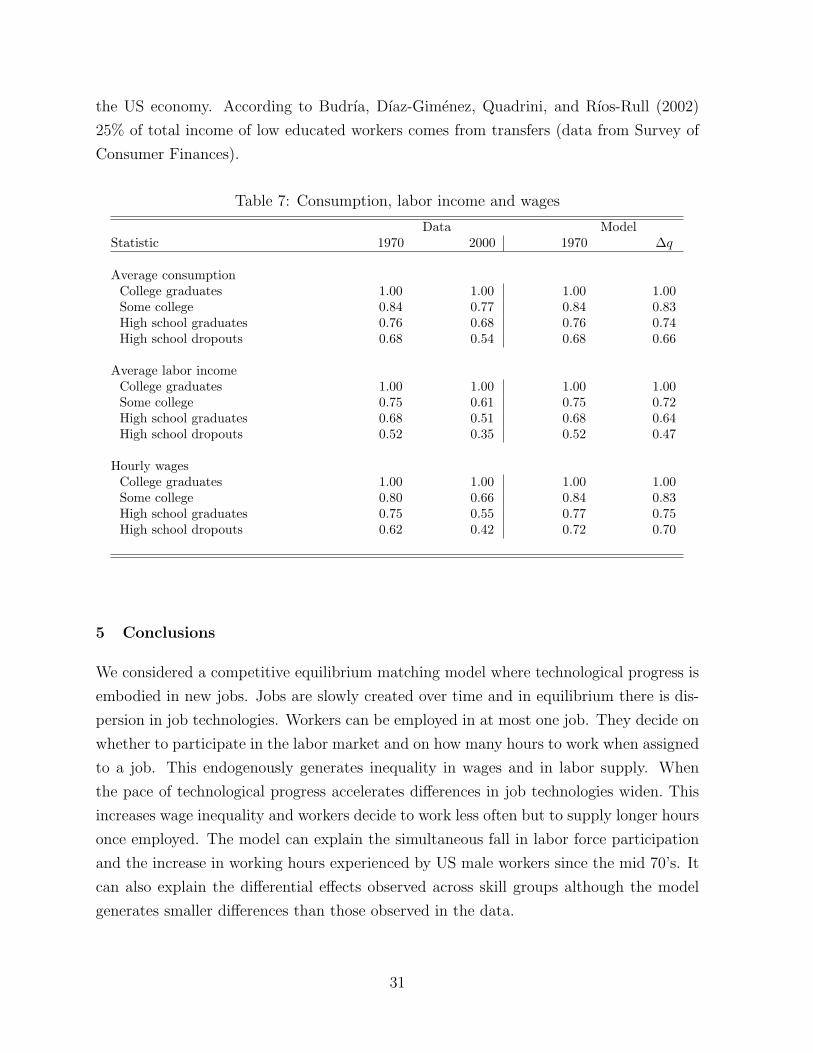
the US economy. According to Budrıa, Dıaz-Gimenez, Quadrini, and Rıos-Rull (2002)

25% of total income of low educated workers comes from transfers (data from Survey of

Consumer Finances).

Table 7: Consumption, labor income and wages

Data ModelStatistic 1970 2000 1970 ∆q

Average consumptionCollege graduates 1.00 1.00 1.00 1.00Some college 0.84 0.77 0.84 0.83High school graduates 0.76 0.68 0.76 0.74High school dropouts 0.68 0.54 0.68 0.66

Average labor incomeCollege graduates 1.00 1.00 1.00 1.00Some college 0.75 0.61 0.75 0.72High school graduates 0.68 0.51 0.68 0.64High school dropouts 0.52 0.35 0.52 0.47

Hourly wagesCollege graduates 1.00 1.00 1.00 1.00Some college 0.80 0.66 0.84 0.83High school graduates 0.75 0.55 0.77 0.75High school dropouts 0.62 0.42 0.72 0.70

5 Conclusions

We considered a competitive equilibrium matching model where technological progress is

embodied in new jobs. Jobs are slowly created over time and in equilibrium there is dis-

persion in job technologies. Workers can be employed in at most one job. They decide on

whether to participate in the labor market and on how many hours to work when assigned

to a job. This endogenously generates inequality in wages and in labor supply. When

the pace of technological progress accelerates differences in job technologies widen. This

increases wage inequality and workers decide to work less often but to supply longer hours

once employed. The model can explain the simultaneous fall in labor force participation

and the increase in working hours experienced by US male workers since the mid 70’s. It

can also explain the differential effects observed across skill groups although the model

generates smaller differences than those observed in the data.

31

A Theorems and proofs

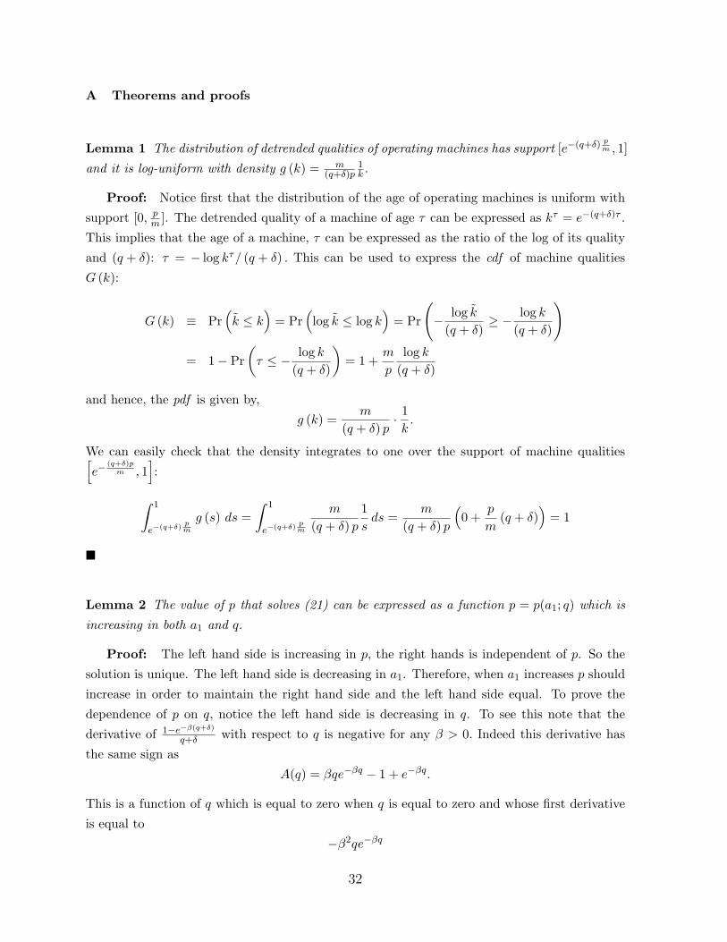
Lemma 1 The distribution of detrended qualities of operating machines has support [e−(q+δ) pm , 1]

and it is log-uniform with density g (k) = m(q+δ)p

1k .

Proof: Notice first that the distribution of the age of operating machines is uniform with

support [0, pm ]. The detrended quality of a machine of age τ can be expressed as kτ = e−(q+δ)τ .

This implies that the age of a machine, τ can be expressed as the ratio of the log of its quality

and (q + δ): τ = − log kτ/ (q + δ) . This can be used to express the cdf of machine qualities

G (k):

G (k) ≡ Pr(k ≤ k

)= Pr

(log k ≤ log k

)= Pr

(− log k

(q + δ)≥ − log k

(q + δ)

)

= 1− Pr(τ ≤ − log k

(q + δ)

)= 1 +

m

p

log k(q + δ)

and hence, the pdf is given by,

g (k) =m

(q + δ) p· 1k.

We can easily check that the density integrates to one over the support of machine qualities[e−

(q+δ)pm , 1

]:

∫ 1

e−(q+δ)pm

g (s) ds =∫ 1

e−(q+δ)pm

m

(q + δ) p1sds =

m

(q + δ) p

(0 +

p

m(q + δ)

)= 1

�

Lemma 2 The value of p that solves (21) can be expressed as a function p = p(a1; q) which is

increasing in both a1 and q.

Proof: The left hand side is increasing in p, the right hands is independent of p. So the

solution is unique. The left hand side is decreasing in a1. Therefore, when a1 increases p should

increase in order to maintain the right hand side and the left hand side equal. To prove the

dependence of p on q, notice the left hand side is decreasing in q. To see this note that the

derivative of 1−e−β(q+δ)

q+δ with respect to q is negative for any β > 0. Indeed this derivative has

the same sign as

A(q) = βqe−βq − 1 + e−βq.

This is a function of q which is equal to zero when q is equal to zero and whose first derivative

is equal to

−β2qe−βq

32

which is negative. This implies that the quantity A(q) is negative for any q > 0, which proves

that the left hand side of (21) is decreasing in q. �

Lemma 3 When q increases both a0 and a1 fall.

Proof: When q goes up the (FE) condition shifts down while the (IE) condition remains

unchanged. As a result both a0 and a1 fall. To see that the (FE) schedule moves down recall

that Lemma 2 states that holding a1 constant p increases with q; so both p and q move up and

a0 moves down for a given a1. �

Lemma 4 When q increases the quality gap e(q+δ) pm between the best and worst machines in-

creases.

Proof: The quality gap depends on the product (q + δ) p. Let’s combine equations (IE)

and (FE) to obtain the following relationship between q and a1 and p.

a1 =

[λ1 (1− α)

1−αα+η (α+ η)

λ0 (1 + η)

]α+η1+η

e−α(q+δ) pm (43)

Lemma 3 proves that a1 falls when q increases. Hence, (q + δ) p should increase with q for

equation (43) to be satisfied. �

Proposition 5 When q increases p falls and n increases.

Proof: To analyze the effect of q on p notice that Lemma 2 shows that q affects p directly

and indirectly through the effects it exerts on a1, p = p (a1; q). The direct effect is positive,

the indirect effect is negative since p depends positively on a1 (see Lemma 2) while q effects

negatively a1 (see Lemma 3). We will see that the equilibrium effect dominates and p falls when

q increases. To see this let’s substitute a1 in equation (43) into equation (21) to obtain the

following relationship between p and q:

α

λ0=

m

q + δ

[eα(1+η)(q+δ)p

(α+η)m − 1]

(44)

The left hand side is independent of p whereas the right hand side is increasing in p, so p is

uniquely determined. One can also check that the right hand side is increasing in q. Hence, it

immediately follows that an increase in q should be compensated by a fall in p. To see that the

33

right hand side in (44) is increasing in q notice that the sign of the derivative of the right hand

side of the equation with respect to q is the same as that of the derivative of the function

z(x) =eγ0x − 1

x(45)

where γ0 = α(1+η)p(α+η)m > 0. The derivative of this function has the same sign as

g(x) = γ0eγ0xx− eγ0x + 1.

To see that this quantity is positive one can notice that g(0) = 0 and that

g′(x) = (γ0)2 eγ0xx

is positive for any positive x. This completes the proof that the right hand side in (44) is

increasing in q.

To analyze the effect of q on n, use (43) to substitute for a1 in (24). We obtain that n in

(24) is increasing in (q + δ) p. To see this, notice the sign of the derivative of n with respect

to (q + δ) p has the same sign as that of derivative of the function z(x) in (45), which we have

already proved to be increasing in x for any γ0 ∈ (0, 1). Since Lemma 4 proves that (q + δ) p

increases with q, n increases. �

Proposition 6 When q increases labor income inequality as measured by LI increases.

Proof: Lemma 4 shows that (q + δ) p increases with q and Lemma 3 shows that a1 falls

when q increases. To understand the relationship between LI and a1, note that we know that

the function u(x) = x+ax+b is decreasing in x if a > b. Indeed u′(x) has the same sign as

x+ b− x− a < 0.

It immediately follows that LI increases with q. �

Lemma 7 For type i workers, the distribution of detrended qualities of operating machines has

support[k∗i , k

∗i−1

]= [e−(q+δ)τ∗i , e−(q+δ)τ∗i−1 ] and it is log-uniform with density gi (k) = m

(q+δ)pizi1k

Proof: The first part of the Lemma follows directly from Lemma 1. To prove the second

part notice first that the distribution of the age of machines operated by workers of type i is

uniform with support[τ∗i−1, τ

∗i

]. The detrended quality of a machine of age τ can be expressed

as kτ = e−(q+δ)τ . This implies that the age of a machine, τ can be expressed as the ratio of

34

the log of its quality and (q + δ): τ = − log kτ/ (q + δ) . This can be used to express the cdf of

machine qualities Gi (k) for type i workers:

Gi (k) ≡ Pr(k ≤ k

)= Pr

(log k ≤ log k

)= Pr

(− log kq + δ

≥ − log kq + δ

)

= 1− Pr(τ ≤ − log k

q + δ

)= 1−

∫ − log kq+δ

τ∗i−1

1τ∗i − τ∗i−1

ds

= 1 +m

pizi

(log kq + δ

− τ∗i−1

)and hence, the pdf is given by,

gi (k) =m

(q + δ) pizi· 1k.

We can easily check that the density integrates to one over the support of machine qualities

[e−(q+δ)τ∗i , e−(q+δ)τ∗i−1 ]:

∫ e−(q+δ)τ∗i−1

e−(q+δ)τ∗i

gi (s) ds =∫ e

−(q+δ)τ∗i−1

e−(q+δ)τ∗i

m

(q + δ) pizi1sds =

m

(q + δ) pizi

[− (q + δ) τ∗i−1 + (q + δ) τ∗i

]= 1.

�

Lemma 8 π (k, hi) ≥ π (k, hj) for k ∈[k∗i , k

∗i−1

]and i < j if and only if the following condition

holdscjci≥(hjhi

)( 1−θθ )(1+η)

Proof: Note that the free entry conditions (39) states that π (k, hi) = π (k, hj) whenever

j = i+ 1 and k = k∗i . The inequality of the lemma will be met if and only if as capital quality

increase, profits increase more for the firm with the better worker. That is to say, we require,

∂π (k, hi)∂k

≥ ∂π (k, hj)∂k

Going to the profit function (30) and the output function (29) we see that the above inequality

requires,h

(1−α)(1−θ)Ai

aA−11,i

≥h

(1−α)(1−θ)Aj

aA−11,j

Finally, equation (17) gives an expression for a1,i and a1,j as a function of consumption that

leads to,cjci≥(hjhi

)( 1−θθ )(1+η)

�

35

B Derivation that output is equal to consumption from first principles.

One can derive this result from first principles. Let’s

Ni ≡ ρ∫ ∞

0e−ρτ

n1+ητi

1 + ηI (nτi > 0) dτ

denote a permanent lifetime measure of work effort for worker i where I (s > 0) denotes the

indicator function and nτi denotes detrended hours of individual i. Finally let’s

N =∫ 1

0Nidi

denotes a permanent lifetime measure of aggregate work effort in the economy. After substituting

the wage function (13) into equation (16) and after using (14) to replace the interest rate,

integrating with respect to i over the unit interval yields

c0 = a0p+ a1N + Π

where p =∫ 1

0 I (nτi > 0) di is the participation rate which is constant over time and

Π = p

∫ 1

e−qpm

π(s)g (s) ds =α+ η

1 + ηY − a0p (46)

are aggregate profits.

We can use (19) to obtain

N =ρ

1 + η

∫ ∞0

e−ρt(∫ p

0n1+ηi,t di

)dt =

m

q

(1− αa1

) 1+ηα+η α+ η

α (1 + η)2

[1− e−

α(1+η)qp(α+η)m

](47)

which given the definition of aggregate output in (20) can be expressed as

a1N =1− α1 + η

Y. (48)

Together with (46) this immediately implies that

c0 = a0p+ a1N + Π =m

q

(1− αa1

) 1+ηα+η α+ η

α (1 + η)

[1− e−

α(1+η)qp(α+η)m

]= Y,

which means that the good market clears.

36

C General model

Output is produced by combining different intermediate goods according to a Cobb Douglas

production function:

Y = eR 10 ln ysds.

We call sector s as an occupation. The price of each intermediate good is therefore

ps =Y

ys

Workers differ in their skill. Skill is occupation specific and a worker can produces just in one

specifc occupation.. We assume that in each occupation s there are Ns types of skills that

belong to the set Hs = {h1s, h2s....hNss} with relative mass probability {z1s, z2s, ...zNss} with∑Nsj=1 zjs = Zs where Zs is teh maximum amount of workers employed in occupation s. We start

assuming that Ns = N, ∀s and Zs = Z = 1,∀s. There are perfect financial markets and two

types of assets: claims on firm profits and frictionless capital. Given the absence of aggregate

risk both assets yield the same return. In each occupation there are machines of different quality.

Individual have an initial level of wealth which is express as µ of aggregate wealth. We assume

that µ is related to workers human capital according to

µj =1N·(a+ 2b

j

1 +N

), j = 1, 2, ..N

where∑N

11N ·(a+ 2b j

1+N

)= 1, so that

a+ b = 1.

When b is positive more skilled workers starts with greater wealth when b is negative the opposite

is true. b equals to zero means that all individuals start with the same wealth level. Production

requires a match of a worker with a firm. It yields output equal to

y = καe1−α

We assume that workers with human capital h supply efficiency units of labour according to

e = h1−θi nθ, i = 1, 2, ..N.

Capital in the job is given by

κ = kηsx1−ηs

where ηs is occupation specific and x denotes frictionless capital. k is friction capital. The pa-

rameter ηs characterizes the importance of the matching problem that differs across occupation.

37

This specification allows the existence of a steady state with constant growth. We will have that

income in all occupation grows at the same rate. If we were to assume a production function

different from Cobb-Douglas differences in η will translate in different growth rates and there

would no longer exist an interest rate such that the capital market clear. In this specification

consumption growth is identical across individuals.

Profits for a firm in sector j with a job with technology k are given by

π(j, k) = maxx,h,n

pj(kηjx1−ηj

)α (h1−θi nθ

)1−α− (r + δ)x− wj(h, n)

we guess that

wj(h, n) = wj(e)

This guess is verified because

dwj(h,n)dh

dwj(h,n)dn

=dwj(h,n)

dhdwj(h,n)

dn

=β

1− βn

h

Under this guess the firm problem become equal to

π(j, k) = maxx,e

pj(kηjx1−ηj

)α (e)1−α − (r + δ)x− wj(e)

so x solves

x =

[pjα(1− ηj)kαηj (e)1−α

r + δ

] 11−α(1−ηj)

so that

π(j, k) = maxeAj (pj)

11−α(1−ηj) k

αηj1−α(1−ηj) e

1−α1−α(1−ηj) − wj(e)

where

Aj = [1− α(1− ηj)][α(1− ηj)r + δ

] 11−α(1−ηj)

Notice that αηj1−α(1−ηj) + 1−α

1−α(1−ηj) = 1. Notice that changes in α and in ηj have different effects.

ηj = 0 means that there is no assignment problem,ηj = 1 means that assignment problem is

severe.

For simplicity we work with the model without trend. Workers with different skills will be

offered different wage schedule. It is easy to guess that the wage schedule for workers of type i

will be given by

w (n, hi) =

{a0(hi) + a1(hi)n

1+η

1+η , if n > 0

0 if n = 0(49)

Below we will sometimes use the notation aji ≡ aj(hi) for j = 0, 1 and i = 1, 2. Let pi = p(hi)

38

denotes the participation rate of workers of type i.Then the maximal duration of a machine

operated by workers of type one will be given by

τ∗1 =p1z1

m

while workers of type two will operate machine with age greater than τ∗1 and smaller that

τ∗2 =p1z1 + p2z2

m.

In compact form we have

τ∗i =

∑ij=0 pjzj

m

where we define τ∗0 = 0 and p0z0 = 0.

39

References

Aaronson, S., B. Fallick, A. Figura, J. Pingle, and W. Wascher (2006): “TheRecent Decline in Labor Force Participation and its Implications for Potential LaborSupply,” Division of Research and Statistics Board of Governors of the Federal ReserveSystem.

Becker, G. S. (1965): “A Theory of the Allocation of Time,” Economic Journal, 75,493–517.

(1973): “A Theory of Marriage: Part 1,” Journal of Political Economy, 81,813–46.

Budrıa, S., J. Dıaz-Gimenez, V. Quadrini, and J.-V. Rıos-Rull (2002): “NewFacts on the U.S. Distribution of Earnings, Income and Wealth,” Federal Reserve Bankof Minneapolis Quarterly Review, 26(3), 2–35.

Costa, D. (2000): “The Wage and the Length of the Work Day: from 1890s to 1991,”Journal of Labor Economics, 18, 156–181.

Eckstein, Z., and E. Nagypal (2004): “The Evolution of U.S. Earnings Inequality:1961-2002,” Federal Reserve Bank of Minneapolis Quarterly Review, 28(2), 10–29.

Gonzales–Chapela, J. (2007): “On the price of recreation goods as a determinant ofmale labor supply,” Journal of Labor Economics, 25(4), 795824.

Gottschalk, P., and T. Smeeding (1997): “Cross-National Comparisons of Earningsand Income Inequality,” Journal of Economic Literature, 35, 633–687.

Greenwood, J., Z. Hercowitz, and P. Krusell (1997): “Long-Run Implications ofInvestment-Specific Technological Change,” American Economic Review, 87(3), 342–62.

Greenwood, J., and M. Yorokoglu (1997): “1974,” Carnegie-Rochester Series onPublic Policy, 46(2), 49–95.

Heathcote, J., F. Perri, and G. Violante (2009): “Unequal We Stand: An Em-pirical Analysis of Economic Inequality in the United States, 1967- 2006,” Mimeo.

Heathcote, J., K. Storesletten, and G. Violante (2008): “The MacroeconomicImplications of Rising Wage Inequality in the US,” Mimeo, New York University.

Hornstein, A., P. Krusell, and G. Violante (2007): “Technology-Policy Interac-tion in Frictional Labor Markets,” Review of Economic Studies, 74(4), 1089–11124.

Jovanovic, B. (1998): “Vintage Capital and Inequality,” Review of Economic Dynamics,1, 497–530.

40

Juhn, C. (1992): “Decline of Male labor Market Participants: The Role of DecliningMarket Opportunities,” Quarterly Journal of Economics, 107(1), 79–121.

Juhn, C., and S. Potter (2006): “Changes in Labor Force Participation in the UnitedStates,” Journal of Economic Perspectives, 20(3), 27–46.

Katz, L. F., and D. H. Autor (1999): “Changes in the wage structure and earningsinequality,” in Handbook of Labor Economics, ed. by O. Ashenfelter, and D. Card, vol. 3.Elsevier Science Publishers.

Kendrick, J. W. (1961): Productivity Trends in the United States. Princeton UniversityPress, Princeton, NJ.

Krueger, D., and F. Perri (2006): “Does Income Inequality Lead to ConsumptionInequality? Evidence and Theory,” Review of Economic Studies, 73(1), 163–193.

Kuhn, P., and F. Lozano (2005): “The Expanding Workweek? Understanding Trendsin Long Work Hours among U.S. Men, 1979-2004,” NBER Working Paper 11895.

McGrattan, E., and R. Rogerson (2004): “Changes in Hours Worked, 1950-2000,”Federal Reserve Bank of Minneapolis Quarterly Review, 28(1), 14–33.

Mincer, J. (1962): “Labor Force Participation of Married Women: A Study of LaborSupply,” in Aspects of Labor Economics, ed. by H. G. Lewis, pp. 49–82. PrincetonUniversity Press, Princeton, NJ.

Nadiri, I., and I. Prucha (1996): “Estimation of the Depreciation Rate of Physical andR&D Capital in the U.S. Total Manufacturing Sector,” Economic Inquiry, 34, 43–56.

Prescott, E., R. Rogerson, and J. Wallenius (2006): “Lifetime Aggregate LaborSupply with Endogenous Workweek Length,” Unpublished manuscript, Arizona StateUnivresity.

Sattinger, M. (1975): “Comparative Advantage and the Distributions of Earnings andAbilities,” Econometrica, 43, 455–68.

Vandenbroucke, G. (2008): “Trends in Hours: The U.S. from 1900 to 1950,” Journalof Economic Dynamics and Control, forthcoming.

Violante, G. (2002): “Technological Acceleration, Skill Transferability and the Rise ofResidual Inequality,” Quarterly Journal of Economics, 117, 297–338.

Whaples, R. (1990): “The Shortening of the American Work Week: An Economic andHistorical Analysis of its Context, Causes, and Consequences,” Ph.D. thesis, Universityof Pennsylvania.

41