Labor Earnings Inequality in Manufacturing During the ...

Labor Earnings Inequality in ManufacturingDuring the Great Depression ∗

Felipe BenguriaUniversity of Kentucky

[email protected]

Chris VickersAuburn University

[email protected]

Nicolas L. ZiebarthAuburn University and NBER

[email protected]

September 21, 2018

Abstract

We study labor earnings inequality in manufacturing during the Great Depres-sion using establishment-level information from the Census of Manufactures. Between1929 and 1933, the difference in log earnings between the 75th and 25th percentiles ofthe establishment wage distribution decreases by 10 log points. By 1935, the 75-25difference is almost back to its 1929 level. Nearly all of these changes in the overalldistribution are from changes in the blue collar earnings distribution. Dispersion inhourly wages declines between 1929 and 1935, with the convergence of the South inhourly wages stronger than that observed in annual earnings.

∗We thank participants at the NBER SI 2015 DAE, Census Bureau, William & Mary, UW-La Crosse,Florida State, Gettysburg College, Northwestern University, EBHS 2017, the Washington Area EconomicHistory Seminar, and the University of Michigan for useful comments. We thank Dave Donaldson, RickHornbeck, and Jamie Lee for providing county-level data for the 1929 Census of Manufactures. We thankMiguel Morin for providing the transcription of some of the published totals for the 1935 Census of Manufac-tures. The National Science Foundation (SES #1122509 and #1459263) and the University of Iowa providedfunding.

1

1 Introduction

The Great Depression is still to this day the largest downturn in American economic his-

tory. While changes in aggregates such as output and prices are well known, even if their

causal explanations are still hotly debated, much less is known about the distributional

consequences of the Depression. This gap in our understanding of these distributional

changes is striking given the growing interest in the role played by short-run economic

fluctuations in the dynamics of earnings inequality. For example, Guvenen et al. (2014)

document larger losses in earnings for lower-income households during recent U.S. reces-

sions compared to higher-income ones.

To address this gap, we draw on establishment-level data from 25 industries from the

Census of Manufactures between 1929 and 1935 to study the effects of the Depression

on earnings inequality. Our use of labor demand side information is motivated by data

availability, but recent work has emphasized the role of firm or establishment character-

istics in determining the earnings distribution (Card et al., 2013; Barth et al., 2016; Song

et al., 2015). Our sample of industries, while not randomly chosen, covers a wide swathe

of manufacturing, from durable goods to consumer products to “high tech” industries.

A key feature of this Census is its frequency: We have transcribed schedules from 1929,

1931, 1933, and 1935, allowing us to study income dynamics from the beginning of the

Depression through its nadir and the first part of the recovery. For each establishment, we

observe the earnings of wage earners and of salaried workers, which we refer to as blue versus

white collar workers. This distinction is very close to that between production and non-

production workers commonly used today in working with manufacturing establishment

data, e.g., Davis and Haltiwanger (1991).1

Our first result is that those in the bottom of the earnings distribution who remained

employed gained relative to the median over the first half of the 1930s. In fact, the difference1To support the claim that this distinction is related to skill as measured by educational differences,

we show that there is a positive relationship between educational attainment and the share in white collaremployment using data from the 1940 Population Census.

2

in the 75th and 25th percentiles declines by 10 log points between 1929 and 1933 with a

decline of a similar magnitude in the difference between the 90th and 10th percentiles.

However, by 1935, the 75-25 difference is nearly back to its 1929 (pre-Depression) level

while the 90-10 difference declines further from its 1933 level. These changes are driven

by shrinking gaps between the bottom and median of the distribution offsetting widening

gaps between the top of the earnings distribution and the median. In particular, the 90-50

difference increases by 22 log points between 1929 and 1933 before falling 25 log points

from 1933 to 1935. On the other hand, the 50-10 difference declines 30 log points between

1929 and 1933 before increasing 10 log points from 1933 to 1935. Changes in the earnings

distribution for blue collar workers account for the nearly all of the changes in the overall

earnings distribution. This is not only due to the fact they make up around 90% of the

workers covered by our sample, but also because the while collar earnings distribution

shows very little change over this six year period.

Our second result is that changes in annual earnings likely understate the decline in

inequality adjusted by hours worked among the employed. The early Depression saw

sharp declines in the length of the workweek, both for economic reasons and as a result of

the National Industrial Recovery Act (NIRA) of 1933. To understand the impacts of these

changes in hours, for 1929 and 1935, we take advantage of a question about the “typical”

workweek at a given establishment to estimate an establishment’s average hourly wage.2

We find that there is a pronounced decline in wage inequality, driven again by the bottom

of the distribution. While the 90-50 gap declines by only 3 log points between 1929 and

1935, the 50-10 gap declines by 30 log points.

Next, we account for the causes underlying the changes in earnings dispersion by de-

composing changes in the overall distribution into changes in observables, returns to those

observables, and unobservables following the procedure in Juhn et al. (1993). We find2Unfortunately, for 1933, a year with large swings in the workweek over the year, we observe only a

workweek number for one week in December. This number is not representative of the year as a whole. Formanufacturing, the average workweek in 1933 was 36.4, but only 33.8 in December (Beney, 1936, Table II).For this reason, we exclude 1933 when we focus on hourly wages.

3

that the initial compression in earnings across establishments is driven almost entirely by

changes in returns to observables: size of the establishment, “collar” color, industry and

region. Changes in the distribution of establishments across these observables, if anything,

act in the opposite direction. Changes in the residuals play no role. Echoing previous re-

sults using industry level data from Rosenbloom and Sundstrom (1999), we find regional

convergence, with low income parts of the country doing relatively better through 1935.

If anything, the changes in regional differences between 1929 and 1935 are even more

pronounced for hourly wages. The reduction in wages associated with being in the South

Atlantic and East South Central regions falls by 29 log points in each region, considerably

more than the changes in annual blue collar earnings. That is, focusing on only changes in

average earnings understates the degree of regional convergence, since it misses a conver-

gence in work hours. The timing of this convergence is consistent with an explanation, at

least partially, driven by the NIRA. While this law was invalidated in May 1935, its provi-

sions for job sharing would have at affected hours worked and earnings in our last sample

period. Wright (1997) also points to the NIRA as a key driver of regional convergence but

focuses on the NIRA-imposed minimum wages. On the other hand, our results before

the NIRA is enacted highlight that regional convergence is not simply due to this policy

change.

In order to reconcile the differences in patterns for annual earnings and hourly wages,

we examine establishment characteristics that determine the length of the workweek. The

most striking finding is a large decline in workweeks in the South relative to the North.

While in 1929 workweeks in southern regions were up to 10 log points above those in New

England, by 1935 they are, if anything, shorter. There is some limited evidence of com-

pression in the distribution of the workweek, as the 75-25 difference declines. This change

is driven by changes in the coefficients associated with establishment characteristics, in

particular the relationship between geography and the length of the workweek.

While there are clear strengths of our dataset, it is also important to keep in mind its

4

limitations and their effects on the interpretation of our results. First, our data are re-

stricted to manufacturing. This is similar to the work of Davis and Haltiwanger (1991),

who study earnings dispersion between and across manufacturing plants during 1963-

1986. Second, the changes in inequality we measure are for the employed, as is the norm

in the literature on earnings dispersion within and across firms (Card et al., 2013; Barth et

al., 2016; Song et al., 2015). The Great Depression is a period of high levels of unemploy-

ment and, for that reason, taking these extensive margin changes into account would be

crucial for extrapolating our findings to inequality including the unemployed. Third, as

we noted earlier, we observe hours worked only imperfectly, though this is not unusual in

the earnings inequality literature, e.g., Song et al. (2015).

It is interesting to compare these results to the longer-run trends in 19th century wage

dispersion documented by Atack et al. (2004). They show that inequality in establishment

wages increases between 1850 and 1880, and, using the same decomposition, changes in

returns to observables play almost no role. Instead, the residual or unmeasured com-

ponent explains about 2/3 of the change in the 90-10 differential and the establishment

characteristics the remaining fraction. Their explanation for these results is based on the

rise of mass production and an increasing concentration of workers at the largest estab-

lishments.3 Our results suggest that as supply-side determinants of inequality such as

education and technology vary at longer frequencies, workplace characteristics may play

a larger role in explaining inequality at business cycle frequencies.

Our results also provide an important additional datapoint on the trajectory of Ameri-

can income inequality over the first half of the 20th century. The Depression happens just

before the U.S. economy experienced a remarkable compression in wages by skill (Goldin

and Margo, 1992) and a decline in the share of income going to the highest earners (Piketty

and Saez, 2003), and just after a substantial increase in inequality during the 1920s.4 Based3One difference between this study and ours is the frequency of the data. They observe establishments

every decade, while we are looking at a two-year frequency.4There are data limitations that have hampered earlier work on this period. Data drawn from tax records

that is the basis for the paper by Piketty and Saez (2003) are useful only to compare those at the very top

5

on the fact that the earnings distribution in 1935 looks quite similar to that in 1929, we

would argue that, at least, the first half of the Depression, a time spanning not just eco-

nomic but also political upheavals, is not associated with persistent declines in labor earn-

ings inequality.5

1.1 Related Literature

Most of the literature on inequality has focused on worker characteristics such as educa-

tional attainment in explaining earnings differences. This is not because workplaces are

unimportant. Work going back to Groshen (1991) has argued just the opposite. Instead,

lack of detailed information on workplaces has limited what can be said about the role

of demand side for labor in generating earnings dispersion. This has begun to change

with the availability of establishment-level datasets such as the Census of Manufactures.

For example, Davis and Haltiwanger (1991) document that over half of wage variance in

manufacturing can be accounted for by dispersion across establishments in mean earn-

ings. Moreover, dispersion across establishments accounted for almost half of the overall

growth in wage dispersion in manufacturing between 1975 and 1986. More recently, Song

et al. (2015) use tax records to show that within-firm wage differentials have changed far

less than between-firm ones over the last 30 years. Barth et al. (2016) find that the increase

in inequality in recent decades is mostly a between-firm phenomenon. Using German

linked employer-employee data, Card et al. (2013) show that changes in inequality in re-

cent decades are due to larger dispersion of worker effects, larger dispersion of firm effects,

and increased assortative matching between workers and firms.

As for earlier work on changes in inequality during the Great Depression, most earlier

relative to the rest of the population, since the vast majority of the population did not then pay incometaxes.The Population Census was conducted only once per decade and did not include wage data until1940. The Bureau of Labor Statistics (BLS) conducted occasional surveys during the Depression, but theydo not allow for systematic measures of wage inequality across industries and states.

5We do not think this claim necessarily contradicts those in Piketty and Saez (2003), who focus on in-equality in total taxable income.

6

work has focused on the geographic dimension mainly for data availability reasons. For

example, Hanna (1954), Schmitz and Fishback (1983), and Creamer and Merwin (1942)

all consider changes in earnings across states during this period. Rosenbloom and Sund-

strom (1999) document that different regions of the country do better or worse during the

Depression, at least as measured by manufacturing outcomes, even after controlling for

differences in industry composition. Hausman (2016) shows that much of the geography

of the 1937 recession is explained by industry differences, particularly the sharp decline in

the automobile industry. Drawing on BLS data, Wallis (1989) documents variation in state

level employment outcomes, which he argues are not mainly driven by industry differ-

ences. In an earlier paper, Borts (1960) also documents the regional variation in business

cycles across the country. Much of the other work on inequality (Kuznets, 1953; Goldsmith

et al., 1954; Tucker, 1938) uses the published statistics on income based on income tax re-

turns and attempts to infer some measure of inequality from that and aggregate income.

These methods are limited to only focusing on inequality driven mainly by the upper in-

come percentiles. Mendershausen (1946) uses the Financial Survey of Urban Housing,

which contains city level information about income in 1929 and 1933.

There are also a handful of papers that focus on industry differences during the De-

pression, including the classic work by Bernanke (1986). He studies a sample of eight

industries with information on employment and wages, drawing on data first studied by

Beney (1936). Hanes (2000), following work by Shister (1944) and Dunlop (1944), exam-

ines industry characteristics and their relationship to wage rigidity during the Depression

and two other downturns in 1893 and 1981. Goldin and Margo (1992) have some data on

the skill premium in a handful of industries that cover the period of the Great Depression.

Clearly, differences in wage rigidity with respect to declines in labor demand will generate

cyclical changes in inequality, though this aspect is not drawn out in that work. The source

for the data in that work is a BLS survey of establishments. Other work by Wachter (1970)

has examined more generally the cyclical variation in the distribution of wages across in-

7

dustries. There is no literature that we are aware examining the role of establishment or

worker level characteristics for understanding inequality during the Great Depression.

Our work also contributes to an emerging literature on inequality during the 2008-2009

Great Recession. Mian and Sufi (2016) survey the literature on the distributional conse-

quences of recessions, and provide further evidence on the role of pre-recession house-

hold debt as a determinant of consumption losses. Heathcote et al. (2010) and Guvenen

et al. (2014) show that in all U.S. recessions in recent decades earnings fall substantially

more for those at the bottom quantiles of the pre-recession earnings distribution, widen-

ing inequality.6 Saez (2015) also documents earnings growth in the U.S. during the Great

Recession for various percentiles of the income distribution.

2 Data and Data Issues

2.1 Data Source: Census of Manufactures

We employ the Census of Manufactures (COM), for which the original, establishment-

level schedules are available from 1929, 1931, 1933, and 1935. The COM was taken for

other years, including during the Depression, but the establishment-level schedules from

the first half of the 20th century do not exist other than for these four years. The schedules

provide a wealth of detail beyond simply identifying information and include a break-

down of outputs and inputs into quantities and values. For our purposes, there is also

information on labor use broken down by type of worker, number employed, and total

earnings.

This work draws on a sample of 25 industries summarized in Table 1.7 In Table 2, we

compare the totals in the data used in this paper to the national published tables along

various dimensions. The sample comprises over 20% of the total value of output in manu-6An exception occurs at the top percentile, which also sees very large losses during the Great Recession.

Parker and Vissing-Jorgensen (2010) discuss the changing cyclicality of top income shares.7These data are from ICPSR Study 37114 (Vickers and Ziebarth, 2018).

8

facturing, approximately 10% of the establishments, and about 20% of both the total wage

bill. While not chosen to be representative, these industries do cover a wide variety of

manufactured products from durables to consumer goods to “high tech” goods like ra-

dios. In addition, there are large differences across the sample in terms of the average size

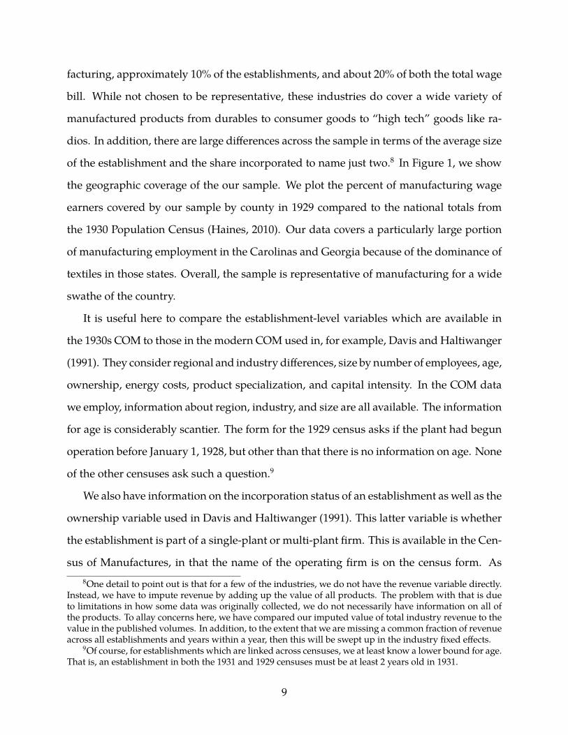
of the establishment and the share incorporated to name just two.8 In Figure 1, we show

the geographic coverage of the our sample. We plot the percent of manufacturing wage

earners covered by our sample by county in 1929 compared to the national totals from

the 1930 Population Census (Haines, 2010). Our data covers a particularly large portion

of manufacturing employment in the Carolinas and Georgia because of the dominance of

textiles in those states. Overall, the sample is representative of manufacturing for a wide

swathe of the country.

It is useful here to compare the establishment-level variables which are available in

the 1930s COM to those in the modern COM used in, for example, Davis and Haltiwanger

(1991). They consider regional and industry differences, size by number of employees, age,

ownership, energy costs, product specialization, and capital intensity. In the COM data

we employ, information about region, industry, and size are all available. The information

for age is considerably scantier. The form for the 1929 census asks if the plant had begun

operation before January 1, 1928, but other than that there is no information on age. None

of the other censuses ask such a question.9

We also have information on the incorporation status of an establishment as well as the

ownership variable used in Davis and Haltiwanger (1991). This latter variable is whether

the establishment is part of a single-plant or multi-plant firm. This is available in the Cen-

sus of Manufactures, in that the name of the operating firm is on the census form. As8One detail to point out is that for a few of the industries, we do not have the revenue variable directly.

Instead, we have to impute revenue by adding up the value of all products. The problem with that is dueto limitations in how some data was originally collected, we do not necessarily have information on all ofthe products. To allay concerns here, we have compared our imputed value of total industry revenue to thevalue in the published volumes. In addition, to the extent that we are missing a common fraction of revenueacross all establishments and years within a year, then this will be swept up in the industry fixed effects.

9Of course, for establishments which are linked across censuses, we at least know a lower bound for age.That is, an establishment in both the 1931 and 1929 censuses must be at least 2 years old in 1931.

9

for other variables emphasized by Davis and Haltiwanger (1991), we have information for

energy sales for 1929 and 1935 only. Davis and Haltiwanger (1991) employ a measure of

product specialization, which is the fraction of establishment shipments accounted for by

the largest five-digit SIC product class. The most important omission from the COM data

is a measure of capital, which is by and large absent. There are, in some cases, industry-

specific measures of physical capital stock; for example, the amount of compression ca-

pacity in the manufactured ice industry. However, nothing is systematic enough to use in

regressions pooling across industries and years.

2.2 Skill Categories and their Comparability Across Years

A key question is how to measure skill. The forms do not provide any information on, for

example, educational attainment of workers. Instead, we will distinguish between wage

versus salaried employees, or what we will call blue versus white collar jobs. White col-

lar workers in this classification were clerks, administrative officers, and office workers in

general. Blue collar workers were presumably mainly production workers on the factory

floor, but they could also include hourly janitorial staff or workers on the loading dock.

In the modern COM, the labor force breakdown is into production and non-production

workers. Dunne et al. (1997) defend the use of non-production workers as a measure of

skilled workers. Our breakdown is quite similar to this. All of our salaried workers would

fall into the category of non-production workers. However, there are surely some hourly

workers such as janitors that would be classified as non-production workers in the modern

taxonomy. We show below that this white versus blue collar distinction carries consider-

able information about a worker’s educational attainment. For this reason, our results

speak to changes in the skill premium, at least in the context of manufacturing.

There are some additional details worth mentioning for how we construct these em-

ployment variables. For blue collar workers, in all four censuses, the form asks for the

number of wage earners employed in each month. The income measure comes from a

10

question asking for “total amount paid to wage earners.” So in computing blue collar av-

erage earnings, we take the total amount paid divided by the average of the monthly em-

ployment figures to compute the average income. Note that “blue collar” here does not

refer to strictly speaking “unskilled” labor. The census forms in 1929 and 1933 ask es-

tablishments to include “skilled and unskilled workers of all classes, including engineers,

firemen, watchmen, packers, etc.” along with “foremen and overseers in minor positions

who perform work similar to that done by the employees under their supervision.” The

question for these group in 1935 was somewhat different, asking respondents to include

“all time and piece workers employed in the plant”, not including employees included in

the other enumerated categories of officers, managers, clerks, and “technical employees.”

As noted by Rosenbloom and Sundstrom (1999), the Census itself cautioned about how

to interpret the wage earner employment number, our measure of blue collar employment.

In particular, they listed some possible reasons why the employment numbers are inflated

relative to the “true” number of full-time equivalent employees. First, the establishments

might have reported part-time workers as well. Second, workers that were laid off might

have stayed on the payroll for a time and still been potentially counted as working at the es-

tablishment. While these may potentially bias the overall level of average earnings, identi-

fying systematic biases they would create in cross-regional or cross-industry comparisons

is more difficult.

For white collar workers, the computation is somewhat more complex. First, we ex-

clude officers and proprietors from the totals since we have no information about their

earnings. For the remaining white collar workers, in 1929, the census asks about the num-

ber of “managers, superintendents, and other responsible administrative employees; fore-

men and overseers who devote all or the greater part of their time to supervisory duties;

clerks, stenographers, bookkeepers, and other clerical employees on salary”, as well as the

total amount that this group was paid. In 1933, this category is split between the managers

and clerks reported separately, along with their total wage bill, with no mention of fore-

11

men.10 For 1935, the same three white collar categories of officers, managers, and clerks

are reported, with the total number of clerks being reported for four separate months. For

this year, there is also an entry for the number of “technical employees” including “trained

technicians, such as chemists, electrical and mechanical engineers, designers, etc.”, which

is not asked in any other year, along with the income they are paid. We do not include

technical employees in the calculations since they are not included in the previous years.

Unfortunately, the 1931 census form does not contain any information about white collar

workers, only asking about an establishment’s number of wage earners.

2.3 What is the White vs. Blue Collar Distinction Reflecting?

An important question is what our distinction between salaried, white collar, and wage

earners, blue collar, captures. We interpret it as reflecting educational attainment, com-

monly referred to as high versus low skill in the literature. To provide supporting evi-

dence, we turn to the 1940 Population Census. While the COM did not collect information

on the educational attainment of workers, the occupational description and industrial af-

filiation of these white collar and blue collar worker categories can be matched to those in

the Census of Population to obtain information on the characteristics of workers in these

different types of jobs. In particular, IPUMS has coded occupations into 3 digit categories,

with 1 through 300 as corresponding to white collar and the rest corresponding to blue

collar save for occupation 999, which is the code for missing or unclassified.

Overall, pooling together workers in all manufacturing industries and in all states, we

find that in 1940 only 17.2 percent of blue collar workers had an educational attainment

corresponding to a high school degree or more. In contrast, 61.6 percent of white collar

workers had at least a high school degree. The median white collar worker has an edu-

cational attainment of 12 years of school (exactly a high-school degree) while the median10In both 1929 and 1933 the census specifically includes foremen in “minor positions who perform work

similar to that done by the employees under their supervision” in the wage earner category.

12

blue collar worker had 8 years of schooling. Table 3 puts this into a regression framework

and predicts educational attainment based on the white versus blue collar distinction. We

consider two definitions of educational attainment: (1) high school graduate and (2) some

college, employing one specification with no controls and one with controls for sex, race,

industry and state fixed effects. We find a statistically and economically significant rela-

tionship education and white-collar employment. While not as good as directly observing

educational attainment of a worker, this shows that the “color” of a worker’s job carries

considerable information about his educational attainment.

2.4 Earnings Measurement

It is important to clarify our key variable of earnings per worker. We will be comparing

average annual earnings by “collar color” computed by taking total earnings and dividing

by total workers in that type of job at the establishment-level. The term “average” refers

to the fact that this is an average for all workers at a given establishment. This variable

accords with much of the modern literature interested in inequality. One question is how

to handle establishments that report no employees and yet have revenue. These make up

a non-trivial fraction of establishments in our dataset and presumably are cases where the

owner, besides managing the establishment’s operations, also works directly in produc-

tion. Margo (2015) discusses this same problem in the 19th century COM and its effects on

estimates of the returns to scale in the production function. While potentially important

for the question of returns to scale and estimating overall labor income shares, it is not

obvious what the effects of these establishments are on earnings inequality of workers, our

particular interest. One could construct scenarios where the individuals running these

businesses are on average more able and, therefore, their shadow wage is high relative to

the mean of the observed earnings distribution. One might also imagine that because the

owner has to do many different tasks, he is relatively less productive than a worker special-

ized in doing one task. In this case, the shadow wage of the sole proprietor would be low

13

relative to the mean of observed distribution. While both of these theories would affect

the level, it is more difficult to see how they would affect changes in measured inequality

for workers. We have chosen to drop this set of establishments. Finally, all earnings are

measured in 2015$ and the 1% tails are winsorized.11

For blue collar workers, it is possible to infer average hourly earnings using questions

on the “typical” number of hours worked per week. The issue is that these questions re-

garding hours are quite heterogeneous from year to year. They include questions on the

number of shifts, number of hours in operation, as well as the “normal” number of hours

worked in a week. Even the wording of the workweek question changes from year with

the year subtly affecting what is actually being reported. In 1929, the Census asks estab-

lishments to report the “normal number of hours for the individual wage earner” with the

figures based on “practice followed during the year”. In 1933, the question instead asks

for the “number of hours plant was operated (day shift only) during the week including

December 15.” That is, the question is different in asking for the figures for one particular

week rather than the normal practice, as well as asking for the amount the establishment

was operated for the day shift as opposed to the length of the workweek per se. The 1935

form asks for the “normal number of hours per week (day shift only)” though the context

of the form suggests it is referring to establishment operating hours rather than individual

workweeks.

Because of these differences across years, we only calculate average hourly earnings in

1929 and 1935 for blue collar workers using this “normal” hours per week question. In

particular, we construct total hours worked at an establishment as the number of employ-

ees times 50 weeks times the hourly workweek variables. We then divide total earnings

for blue collar employees by this total hours measure to compute our measure of average

hourly earnings for blue collar workers.11Adjustments for inflation are made using the CPI-U price index.

14

3 Changes in the Earnings Distributions

The first panel of Figure 2 shows the overall distribution of earnings pooling blue and

white collar workers where each establishment-“collar” is weighted by the number of

workers. We emphasize that this distribution is not the “true” distribution of worker

earnings in manufacturing, since we are implicitly treating all workers at a given estab-

lishment as earning the same amount. This will surely mask variation in earnings within

an establishment and skill group, so the inequality measures based on this distribution

will be lower than the measures from the distribution where we observed every individ-

ual employee’s earnings. However, the Davis and Haltiwanger (1991) decomposition for

modern data shows over half of the variance in manufacturing wage inequality can be

accounted for by between-establishment differences in average earnings. This suggests

that a substantial fraction of changes in the income distribution can be captured using

establishment-level averages.

The distribution goes from being bimodal in 1929 to unimodal in 1933 and then back

again in 1935. As we show later, this shift is driven by blue collar workers in durable goods

industries. Panel A of Table 4 reports the changes in various differences in percentiles for

this distribution. Focusing on the 75-25 measure of inequality, there is a decline in 10 log

points between 1929 and 1933. By 1935, the 75-25 differential is nearly back to its pre-

Depression 1929 value. We consider this as evidence that the Depression did not have

permanent effects on the “bulk” of the manufacturing earnings distribution as reflected

in the 75-25 differential.

This claim needs to be qualified in two ways. First, the 90-10 inequality measure shows

a decline over this six year period, though this is almost totally concentrated in the distri-

bution of earnings for blue collar workers, a point we return to later. Second, this is the

distribution of earnings for those employed and the Depression is a time of large declines

in the number of people working.12 To think about the effects of changes on this margin,12On the other hand, unless tax data is being used, studies on inequality from this time period are in

15

assume that with probability 1 − p, a person receives 0 income and with complimentary

probability, a person receives income w drawn from distribution F with standard devi-

ation σ. We think of this setup as capturing a case where there is a fixed pool of “man-

ufacturing workers” who work in that sector or are unemployed (and receive nothing).

Then the standard deviation of the earning distribution including those that are unem-

ployed is SD(w) = pσ, or, in log differences, ∆ logSD(w) = ∆ log p + ∆ log σ. We could

estimate ∆ log p as the log change in total manufacturing employment ignoring changes

in the overall population. The second piece ∆ log σ is what we are estimating here. Note

that decreases in p, increases in manufacturing unemployment, all else equal reduce overall

inequality. This is because in our example, all unemployed workers receive earnings of 0.

The same logic would apply if those that became unemployed received an income draw

from some less dispersed distribution (though the effect on changes in overall inequality

would be more muted).

We now decompose the overall earnings into the distributions for blue and white collar

workers in the other panels of Figure 2. Quite clearly, the qualitative changes in the overall

earnings distribution are being inherited from the blue collar earnings distribution. The

1929 and 1935 distributions for white collar are nearly identical. Panels B and C of Table

4 report the changes in the differences in percentiles for these distributions. As is evident

from the figures, the changes in the overall earnings distribution are driven by changes in

the blue collar earnings distribution. This is also due to the fact that on average, an estab-

lishment has about 10 times as many blue collar than white collar workers. So the overall

earnings distribution places much more weight on changes in the blue collar distribution.

We return later to decomposing changes in the earnings distribution into not just the mix

of blue and white collar employees but also the premium for white collar employees and

a residual term.

One question in interpreting these changes in earnings inequality is the role of changes

effect studies of inequality for the employed because of the data sources available. These data are not rep-resentative samples of the population, but of workers e.g., the data from the Conference Board.

16

in hours worked. We already discussed the related issue of extensive margin changes in

hours worked with unemployment increasing sharply during this period. Our focus here

is on the intensive margin, particularly as it relates to differences between blue and white

collar employees. We know that even for people who kept their jobs, hours worked on

average fell during this period. To the extent that increases in earnings inequality are be-

ing driven by increases in hours inequality we are overestimating changes in “welfare”–

inclusive of both earnings and hours worked–inequality since those that are making less

are being “compensated” by working less (even if this is involuntary). Or to put it differ-

ently, changes in earnings inequality might be totally driven by changes in hours inequality

with no change in the hourly wage distribution.

Panel D of Table 4 reports the changes in the distribution of blue collar hourly wages for

1929 and 1935, the only years where we have information on hours worked. We find that

the blue collar wage distribution became more compressed over this period, for both the

75-25 and 90-10 differentials. The changes were larger in magnitude than those observed

for the annual income distribution. Such a disconnect could be due to either an increase

in the dispersion of hours or an increase in the covariance between hours and the hourly

wage. In Panel E of Table 4, we report the changes in the distribution of hours per wage

earner in 1929 and 1935. In 1935, the interquartile range is zero: Both the 75th percentile

and 25th percentile workweeks are 40 hours long. In 1929, there is more dispersion as

measured by the interquartile range. However, when the broader distribution is consid-

ered, the 90-10, 90-50, and 50-10 gaps are all unchanged from 1929 to 1935. Changes in the

dispersion of the workweek seem unlikely to explain the disconnect between the income

and wage measures. As we show below, the change in hours was not uniform across the

country: The workweek declined in the low wage South more than in other regions. This

larger decline in hours for the South to some degree offset the relative gain in hourly wages

for this area, so the overall effects on the income distribution of these regional changes are

somewhat muted.

17

A different margin along which to split the sample is by whether the industry produces

a durable good. It is well known that output of and employment in durable industries are

much more sensitive to fluctuations in aggregate demand than non-durables. Figures 3

and 4 plot the distributions of earnings for blue and white collar employees, respectively,

separating industries that produce a durable good from those that do not. Strikingly, only

for blue collar workers in durable industries do we observe clear shifts in the earnings

distribution over these years with changes in the average and the dispersion. This find-

ing casts doubt on one interpretation of all these results that they are simply driven by

some quirk in how the 1933 COM was collected. That theory could not explain why the

differences in 1933 are only there for blue collar workers in durable goods industries. One

explanation for these differences by durability and skill group is the hours margin and

the practical constraint on how few hours someone is willing to work. So as demand falls,

the remaining employees have their hours slashed down to this practical minimum and,

therefore, the earnings distribution becomes more compressed.

4 Decomposing the Changes in the Earnings Distributions

After identifying some potential drivers of changes in the earnings distribution, we now

decompose the sources of those changes using the procedure developed by Juhn et al.

(1993) (JMP). First, we write the earnings equation as

yit = Xitβt + uit

where yit is the log average real income (in 2015 dollars) for either blue collar or white

collar workers at establishment i in year t, Xit a vector of establishment characteristics

(and whether the earnings corresponds to white or blue collar workers), and a residual

unobserved component uit. Let the distribution function of the residuals be denoted by

Ft(.). Then define establishment i’s percentile in the distribution of residuals as θit. After

18

estimating the regression, we can then invert the residual as

uit = F−1t (θit|Xit)

where F−1t (θit|Xit) is the inverse CDF of the residuals in year t conditional on character-

istics Xit. This allows us to study not just changes in inequality at the mean but through

the whole distribution (Juhn et al., 1993). Following the literature, we will assume that Ft

is independent of X . So we will drop the dependence on Xit.

Changes in the earnings distribution can come from three possible sources: (1) changes

in average establishment characteristics Xit; (2) changes in the relationship between these

characteristics and incomes represented by βt (“prices” in the language of JMP); or (3)

changes in the distribution of residuals Ft. To see this analytically, take 1929 as the base

year and define β̄ = β̂1929 and F̄−1(θit) = F̂−11929(θit). Then we can write

yit = Xitβ̄ +[Xit(βt − β̄) + F̄−1(θit)

]+[F−1t (θit)− F̄−1(θit)

].

If the distribution of residuals and the coefficients β were fixed, then earnings would be

y1it = Xitβ̄ + F̄−1(θit).

So changes in the distribution of y1it are those attributable to changes in the characteristics

of the establishments. Now if the returns coefficients βt can change as well as the value of

the covariates Xit, then earnings are

y2it = Xitβt + F̄−1(θit).

So any additional change in the distribution of y2it relative to y1It is due changes in the

“returns” to the observables. Finally, if we further allow the distribution of residuals to

19

change, then earnings are given by

y3it = Xitβt + F−1t (θit),

which is the actual level of earnings. In this case, any additional changes to y3it = yit rel-

ative to y2it can be attributed to changes in the residuals. It is important to remember that

this is just an accounting decomposition and should not be interpreted structurally. Be-

sides the original paper by JMP, a number of authors working with manufacturing data

have employed this procedure such as Davis and Haltiwanger (1991) using modern COM

data and Atack et al. (2004) using the 19th century COM. In estimating the regression and

constructing the residuals, we “pool” both blue and white collar workers and weight each

establishment-“color” by the number of workers in that group. For the vector of character-

istics, we include the log of revenue, a binary variable for whether or not the establishment

is part of an incorporated firm or not, whether the firm owns multiple establishments or

plants, as well controls for Census regions and industry.

Table 5 shows the results from the regressions for each year pooling both types of work-

ers weighted by the number of employees with robust standard errors. First, and not sur-

prisingly, we find a large skill premium—more precisely, difference in average earnings

between white and blue collar workers—of 34 log points in 1929, increasing to 73 points

in 1933, and falling back to 55 log points. This increase in the skill premium is somewhat

larger than that in prior work. For example, Goldin and Margo (1992) report an increase

between 1929 and 1933 in the ratio of monthly income for clerks to laborers in the railroad

industry of about 21 log points. The smaller change is due to the fact that they find a larger

skill premium in 1929 of around 53 log points. We find no statistically significant effect

of working at an incorporated firm or a multiplant firm in any of the three years. There

is also a significant size premium across all three years, consistent with modern literature

on this question. This is consistent across the years, with the coefficient on (log) revenue

20

0.06 in 1929, 0.07 in 1933, and 0.05 in 1935.13

The overall pattern of the regional differences in average earnings (the New England

region is the excluded category) is as expected, with a large negative earnings effect asso-

ciated with being located in the South and all regions having lower average earnings than

New England. What is striking is the decline between 1929 and 1933 in the penalty for

being in the South, which includes the East and West South Central as well as the South

Atlantic regions. While this convergence of the South relative to New England is consis-

tent with the findings in Wright (1997), the timing is not consistent with his explanation.

He argues that this convergence was due to the minimum wages imposed by the NIRA,

which had relatively more of an effect in the South because of the lower average wages

to start. The problem is that the NIRA was not passed until June 1933, and furthermore,

the minimum wages were set on an industry by industry basis in a so-called “Code of

Fair Conduct.” The vast majority of these codes were not approved until 1934. In addi-

tion, many of them also specified lower minimum wages for establishments operating in

the South.These findings echo the results of Rosenbloom and Sundstrom (1999), who find

that the Depression was comparatively mild in these areas after controlling for industry

composition (and long-run trends).

We now turn to the decomposition using these regressions results. In Figure 5, we

show the values from the JMP decomposition for all workers, taking 1929 as the base year

and defining changes relative to that year.We plot the changes in the 90-10 gap and the

75-25 gap. The four graphs show the four parts of the decomposition: (1) Totals yit, (2)

Observables y1it, (3) Prices y2it, and (4) Residuals y3it. The “Totals” figure replicates the pat-

tern observed in the summary statistics of a fanning out of the earnings distribution in 1933

and then a return to the pre-Depression spread by 1935 in the 75-25 differential. Clearly,

changes in the residuals play absolutely no role, and while quantities matter slightly, the

vast majority of the changes in inequality as measured by the 75-25 differential are driven13In the 19th century, this size gradient was negative (Atack et al., 2004).

21

by changes in prices, or the returns to observables. The fact that prices matter is similar

to the original paper by JMP, who argue that much of the increase in wage inequality be-

tween 1963 and 1989 was due to increases in the returns to skill (though a substantial role

is still played by changes in the residuals). On the other hand, ABM find almost no role

is played by changes in prices in explaining increasing wage dispersion during the 19th

century. Instead 2/3 is due to increasing residual wage dispersion and the rest to changes

in observables.

Because the sharpest changes in the distribution of earnings were for blue collar work-

ers, and particularly in the durable goods industries, we perform the same JMP decom-

position for blue collar workers only, separately by nondurable and durable industries.

Tables 6 and 7 show the regression results for nondurable and durable industries, respec-

tively. The striking differences are in the regional effects with larger penalties for being

in the South and smaller ones for other parts of the country (relative to New England)

in non-durable goods industries and the reverse for durable goods industries. In non-

durable goods industries, the coefficients on low income areas all increase from 1929 to

1933, after which there is a smaller further increase. That is, there was regional conver-

gence in these industries. In durable goods industries, by contrast, there is a decline in the

coefficients on low-income regions from 1929 to 1933, but some reversal of this trend in

two of the three regions, with the other constant.

Turning to the decomposition, we plot the results for non-durable goods industries

and durables in Figures 6 and 7 respectively. The 90-10 ratio is flat for non-durables, while

the 75-25 ratio declines from 1929 and then is stable to 1935. The decomposition suggests

a complicated pattern for inequality: Prices are associated with an increase in the 90-10

ratio and a decrease in the 75-25 ratio. In contrast, residuals are associated with a slight

decline in inequality by 1935. Turning to durables, the prices are associated with declines

both from 1929 to 1933 and from 1933 to 1935. In contrast, residuals are associated with an

increase in inequality measures, particularly the 90-10 ratio, before returning to roughly

22

the same level as in 1929 by 1935.

4.1 Wages

We now turn to examining the changes in the distribution of wages, as opposed to annual

earnings. Recall that we have this information only for the years 1929 and 1935. Table 8

shows the regression results of specifications identical to the ones we estimated for earn-

ings. Notable here are the changes in the regional differences in hourly wages. In partic-

ular, average hourly wages in the South Atlantic and East South Central both increase by

29 log points while the West South Central region increases by 25 log points. This gen-

erates substantial degree of regional convergence, more so than in annual earnings, with

regions all across the country catching up with New England. As with annual earnings,

larger firms are associated with higher wages.

To understand these changes, we estimate a JMP decomposition on the wage distri-

bution. We plot the results of this decomposition in Figure 8. It is clear visually that

residuals play virtually no role whatsoever in the change in the distribution of wages. The

large fall in the 90-10 ratio is more than explained by changes in prices. That is, if the

distribution of employment across observable firm characteristics had remained constant,

the 90-10 ratio would have increased. The same is true for the smaller change in the 75-25

difference: The positive effect of quantities on increasing inequality is counteracted by a

larger-in-magnitude fall in prices.

One way to reconcile the larger degree of regional convergence in wages compared to

that in incomes is if the hours worked variable changed differentially across geographic

regions. To test this, we regress the length of the log workweek on the same set of variables

as above. The results are in Table 9. It is clear that regional convergence in workweeks is

crucial in explaining the disconnect between the results for income compared to those for

wages. Note that in 1929, the South Atlantic, East South Central, and West South Central

regions, conditional on industry and observable firm characteristics, had workweeks 6 to

23

10 log points longer than those in New England. By 1935, two of these three regions had

essentially no difference in workweeks, and the South Atlantic had workweeks 4 log points

shorter than that in New England.

Finally, we perform a decomposition of the changes in workweek with the same spec-

ification as above, to examine changes in the length of workweek at different parts of the

distribution of workweeks. That is, to what degree do observable firm characteristics ex-

plain changes in the length of the workweek at different points in the distribution of work-

weeks? We plot the decomposition in Figure 9. For the 90-10 difference, there is no change

to explain, as the difference was identical in 1929 and 1935. For the 75-25 difference, resid-

uals play almost no role, and the large majority of the change is explained by the changes

in prices on observable firm characteristics. That is, to the degree that workweeks changed

between 1929 and 1935, it is explained by changes in the mean effects associated with es-

tablishment characteristics, and the composition of establishments in the sample. One key

observable characteristic was region and, in particular, being located in the South, where

the workweek became substantially shorter by 1935. There is little evidence for residual

changes in the distribution of workweeks

5 Conclusion

We have documented a number of dimensions of earnings inequality during the Great

Depression drawing on establishment-level data from the COM. The 75-25 differential of

the overall earnings distribution declines between 1929 and 1933 and then recovers by

1935. From an accounting perspective, this is driven by changes in the blue collar earn-

ings distribution and particularly for that type of worker in durable goods industries. The

distribution of earnings for white collar workers is little changed. When decomposing

these results, we find changes in the wage premiums associated with observable charac-

teristics explain the bulk of the changes, particularly for the blue collar workers in durable

24

goods industries.

Whether or not the Depression resulted in a change in inequality is therefore a matter

of interpretation. As conventionally measured, in terms of annual earnings, the transitory

(though lasting for many years) nature of the Depression translated into transitory effects

on inequality, and to understand the long-swings in inequality during the 20th century,

we need to look beyond this particular macroeconomic event to the long-run trends in

technology and the supply of skilled workers (Goldin and Katz, 2009), and to the discon-

tinuous changes in policy that took place during WWII (Piketty and Saez, 2003). However,

as measured by changes in hourly wages, the Depression seemed to have an effect, as there

was a substantial decline in inequality. The disconnect between these two is driven by re-

gional differences in workweek changes: The length of the workweek dropped by more in

the low wage South than the rest of the country, and therefore the convergence in wages

was greater than the convergence in income.

The question then is what were the overall effects of policy, in particular the NIRA,

on changes in earnings inequality. If one took the view that the effects of the NIRA were

mainly through its effects on the workweek and largely orthogonal to wages paid, as in

a perfectly competitive labor market, then this policy prevented regional convergence in

annual earnings from happening more quickly that it would have otherwise by artificially

suppressing the length of the workweek in the lower wage South. This effect has to be

set against the possible effects the NIRA had on reducing regional disparities in hourly

wages themselves through minimum wages. We leave disentangling these possible effects

of policy induced changes in workweeks on income and wages, as well as the implications

of these for understanding inequality in living standards more broadly, for future work.

25

ReferencesAtack, Jeremy, Fred Bateman, and Robert A. Margo, “Skill Intensity and Rising Wage

Dispersion in Nineteenth-Century American Manufacturing,” Journal of Economic His-tory, 2004, 64, 172–192.

Barth, Erling, Alex Bryson, James C. Davis, and Richard Freeman, “It’s Where You Work:Increase in Earnings Dispersion Across Establishments and Individuals in the U.S.,”Journal of Labor Economics, 2016, 34, S67–S97.

Beney, M. Ada, Wages, Hours and Employment in the United States, 1914-1936, National In-dustrial Conference Board, 1936.

Bernanke, Ben S., “Employment, Hours, and Earnings in the Depression: An Analysis ofEight Manufacturing Industries,” American Economic Review, 1986, 76, 82–109.

Borts, George H., “Regional Cycles of Manufacturing Employment in the United States,1914-1953,” Journal of the American Statistical Association, 1960, 289, 151–211.

Card, David, Jorg Heining, and Patrick Kline, “Workplace Heterogeneity and the Rise ofWest German Wage Inequality,” Quarterly Journal of Economics, 2013, 128, 967–1015.

Creamer, Daniel and Charles Merwin, “State Distribution of Income Payments, 1929-1946,” Survey of Current Business, 1942, pp. 18–26.

Davis, Steve J. and John Haltiwanger, “Wage Dispersion Between and Within U.S. Man-ufacturing Plants, 1963-86,” Brookings Papers on Economic Activity. Microeconomics, 1991,1991, 115–200.

Dunlop, John T., Wage Determination Under Trade Unions, Macmillan, 1944.

Dunne, Timothy, John Haltiwanger, and Kenneth R. Troske, “Technology and Jobs: Sec-ular Changes and Cyclical Dynamics,” Carnegie-Rochester Conference Series on Public Pol-icy, 1997, 46, 107–178.

Goldin, Claudia and Lawrence F. Katz, “The Origins of Technology-Skill Complementar-ity,” Quarterly Journal of Economics, 1998, 113, 693–732.

and , The Race Between Education and Technology, Harvard University Press, 2009.

and Robert A. Margo, “The Great Compression: The Wage Structure in the UnitedStates at Mid-Century,” Quarterly Journal of Economics, 1992, 107, 1–34.

Goldsmith, Selma, George Jaszi, Hyman Kaitz, and Maurice Liebenberg, “Size Distri-bution of Income Since the Mid-Thirties,” Review of Economics and Statistics, 1954, 36,1–32.

Groshen, Erica L., “Sources of Intra-Industry Wage Dispersion: How Much Do EmployersMatter?,” Quarterly Journal of Economics, 1991, 106, 869–884.

26

Guvenen, Fatih, Serdar Ozkan, and Jae Song, “The Nature of Countercyclical IncomeRisk,” Journal of Political Economy, 2014, 122, 621–660.

Haines, Michael R., “Historical, Demographic, Economic, and Social Data: The UnitedStates, 1790-2002. ICPSR02896-v3,” Inter-university Consortium for Political and SocialResearch 2010.

Hanes, Christopher, “Nominal Wage Rigidity and Industry Characteristics in the Down-turns of 1893, 1929, and 1981,” American Economic Review, 2000, 90, 1432–1446.

Hanna, Frank A., State Income Differentials, 1919-1954, Duke University Press, 1954.

Hausman, Joshua, “What Was Bad for General Motors Was Bad for America: The AutoIndustry and the 1937-38 Recession,” Journal of Economic History, 2016, 76, 427–477.

Heathcote, Jonathan, Fabrizio Perri, and Giovanni L Violante, “Unequal We Stand: AnEmpirical Analysis of Economic Inequality in the United States, 1967–2006,” Review ofEconomic Dynamics, 2010, 13, 15–51.

Juhn, Chinhui, Kevin M. Murphy, and Brooks Pierce, “Wage Inequality and the Rise inReturns to Skill,” Journal of Political Economy, 1993, 101, 410–442.

Kuznets, Simon, Shares of Upper Income Groups in Income and Savings, NBER, 1953.

Margo, Robert A., “Economies of Scale in Nineteenth Century American ManufacturingRevisited: A Solution to the ’Entrepreneurial Labor Input Problem’,” in William Collinsand Robert A. Margo, eds., Enterprising America: Businesses, Banks, and Credit Markets inHistorical Perspective, University of Chicago Press, 2015.

Mendershausen, Horst, Changes in Income Distribution During the Great Depression, NBER,1946.

Mian, Atif and Amir Sufi, “Who Bears the Cost of Recessions? The Role of House Pricesand Household Debt,” in John Taylor, ed., Handbook of Macroeconomics, Vol. 2, Elsevier,2016, pp. 255–296.

Parker, Jonathan A. and Annette Vissing-Jorgensen, “The Increase in Income Cyclicalityof High-Income Households and Its Relation to the Rise in Top Income Shares,” Brook-ings Papers on Economic Activity, 2010, 41, 1–70.

Piketty, Thomas and Emmanuel Saez, “Income Inequality in the United States, 1913-1998,” Quarterly Journal of Economics, 2003, 118, 1–39.

Rosenbloom, Joshua L. and William A. Sundstrom, “The Sources of Regional Variationin the Severity of the Great Depression: Evidence From US Manufacturing, 1919–1937,”Journal of Economic History, 1999, 59, 714–747.

Saez, Emmanuel, “Striking It Richer: The Evolution of Top Incomes in the United States(Updated With 2014 Preliminary Estimates),” 2015. Unpublished, UC Berkeley.

27

Schmitz, Mark and Price V. Fishback, “The Distribution of the Income in the Great De-pression: Preliminary State Estimates,” Journal of Economic History, 1983, 43, 217–230.

Shister, Joseph, “A Note on Cyclical Wage Rigidity,” American Economic Review, 1944, 34,110–116.

Song, Jae, David J. Price, Fatih Guvenen, Nicholas Bloom, and Till von Wachter, “Firm-ing Up Inequality,” 2015. Unpublished, Stanford University.

Tucker, Rufus, “The Distribution of Income Among Income Taxpayers in the UnitedStates, 1863-1935,” Quarterly Journal of Economics, 1938, 52, 547–587.

Vickers, Chris and Nicolas L. Ziebarth, “United States Census of Manufactures, 1929-1935. ICPSR37114-v1,” Inter-university Consortium for Political and Social Research2018.

Wachter, Michael, “Cyclical Variation in the Inter-industry Wage Structure,” AmericanEconomic Review, 1970, 60, 75–84.

Wallis, John Joseph, “Employment in the Great Depression: New Data and Hypotheses,”Explorations in Economic History, 1989, 26, 45–72.

Wright, Gavin, Old South, New South: Revolutions in the Southern Economy Since the CivilWar, LSU Press, 1997.

28

Table 1: Summary Statistics of the Sample Industries

Industry Establishments Log Employees Incorporated Durable

Beverages 14907 1.35 43.7 0Ice cream 10105 1.52 54.0 0Ice, manufactured 13242 1.57 78.9 0Macaroni 1269 2.18 49.3 0Malt 131 3.09 96.8 0Sugar, cane 279 4.52 71.9 0Sugar, refining 77 6.47 88.3 0Cotton goods 4483 5.08 91.7 0Linoleum 23 6.40 100 1Matches 82 4.98 93.8 0Planing Mills 12582 2.38 66.9 1Bone black 223 3.24 98.1 0Soap 1004 2.44 80.9 0Petroleum refining 1547 4.12 94.9 0Rubber tires 224 5.36 95.2 1Cement 638 4.65 98.6 1Concrete products 5733 1.58 57.5 1Glass 923 5.01 94 1Blast furnaces 329 5.12 100 1Steel works 1720 5.77 98.5 1Agricultural implements 916 3.33 80.4 1Aircraft and parts 379 3.47 92.0 1Motor vehicles 627 5.01 93.9 1Cigars and cigarettes 145 4.23 77.2 0Radio equipment 786 4.03 86.9 1

Notes: All statistics are calculated over the four census years. Establishments is the total number of estab-lishments, Log Employees is the average number of log employees across establishments. Incorporated isthe percentage of establishments that are incorporated. Durable is whether we coded an industry’s productas durable.

29

Table 2: Percent of National Total Covered by Our Sample

Year 1929 1931 1933 1935

Establishments 11.3 10.5 9.91 9.48Total Wages 20.5 18.2 19.0 20.7Value of Product 20.5 18.4 21.0 18.8

Notes: All of the national totals are from the 1935 published report on the Census of Manufactures, whichreported the previous years totals as well.

30

Table 3: Educational Attainment by White Collar Status in 1940 Census

High school graduate Some college

White collar 0.44∗∗∗ 0.41∗∗∗ 0.21∗∗∗ 0.20∗∗∗

(0.01) (0.01) (0.00) (0.00)Controls No Yes No Yes

Observations 30056 30056 30056 30056

Notes: Estimates are from a linear probability model restricting to individuals employed in manufacturingindustries and between ages 20 and 65. Controls include sex, race, age, and age squared as well as state andindustry fixed effects. Standard errors are robust.

31

Table 4: Summary Statistics of the Log Earnings, Wage, and Hours Distributions

Difference Between Percentiles...75-25 75-50 50-25 90-10 90-50 50-10

Panel A: Overall Earnings1929 0.72 0.26 0.46 1.34 0.47 0.871933 0.62 0.33 0.28 1.22 0.69 0.521935 0.70 0.27 0.43 1.11 0.44 0.67

Panel B: Blue Collar Earnings1929 0.72 0.24 0.48 1.27 0.42 0.861933 0.54 0.27 0.27 1.08 0.58 0.501935 0.68 0.24 0.44 1.05 0.40 0.65

Panel C: White Collar Earnings1929 0.39 0.18 0.22 0.83 0.34 0.481933 0.38 0.15 0.23 0.86 0.28 0.571935 0.41 0.16 0.25 0.82 0.28 0.55

Panel D: Blue Collar Hourly Wage1929 0.77 0.28 0.49 1.43 0.50 0.931935 0.68 0.27 0.41 1.10 0.47 0.63

Panel E: Blue Collar Workweek1929 0.14 0.10 0.04 0.29 0.18 0.111935 0.00 0.00 0.00 0.29 0.18 0.11

Notes: The statistics correspond to the difference between the two percentiles listed. Each establishment isweighted by the number of workers in the particular “color” group.

32

Table 5: JMP Regression Results

Average Earnings(1) (2) (3)

White Collar 0.34∗∗∗ 0.73∗∗∗ 0.55∗∗∗

(0.02) (0.02) (0.02)Incorporated -0.00 0.05 0.01

(0.02) (0.05) (0.02)Multiplant Firm 0.01 -0.00 0.02

(0.02) (0.02) (0.02)Revenue 0.06∗∗∗ 0.07∗∗∗ 0.05∗∗∗

(0.00) (0.01) (0.01)Mid-Atlantic -0.07∗∗∗ -0.11∗∗∗ -0.09∗∗∗

(0.02) (0.04) (0.03)East North Central -0.04∗ -0.05 -0.10∗∗∗

(0.03) (0.04) (0.03)West North Central -0.11∗∗∗ -0.19∗∗ -0.15∗∗∗

(0.03) (0.08) (0.05)South Atlantic -0.35∗∗∗ -0.24∗∗∗ -0.20∗∗∗

(0.02) (0.02) (0.02)East South Central -0.41∗∗∗ -0.24∗∗∗ -0.25∗∗∗

(0.03) (0.03) (0.03)West South Central -0.31∗∗∗ -0.28∗∗∗ -0.26∗∗∗

(0.03) (0.04) (0.03)Mountain 0.00 -0.07 0.03

(0.05) (0.05) (0.04)Pacific -0.07∗∗ 0.02 -0.02

(0.03) (0.03) (0.03)Industry Yes Yes Yes

Observations 32139 17269 25201Year 1929 1933 1935

Notes: The earnings variable is log transformed and the 1% tails are winsorized. In addition to white collarstatus, the set of controls include log revenue, dummies for incorporation, and multiplant as well as regionand industry fixed effects. An observation is an establishment and each establishment is weighted by thenumber of employees in a particular “color” group. The excluded region is New England. Standard errorsare robust.

33

Table 6: JMP Regression Results: Blue Collar Average Earnings in Non-durable Industries

Blue Collar Average Earnings(1) (2) (3)

Incorporated -0.01 0.12∗∗ -0.02(0.02) (0.05) (0.02)

Multiplant Firm 0.00 -0.02 0.02(0.01) (0.02) (0.01)

Revenue 0.06∗∗∗ 0.05∗∗∗ 0.06∗∗∗

(0.01) (0.01) (0.01)Mid-Atlantic 0.04 0.04 0.02

(0.03) (0.04) (0.03)East North Central -0.02 -0.06 -0.02

(0.03) (0.04) (0.03)West North Central -0.02 -0.10∗∗ -0.03

(0.03) (0.04) (0.03)South Atlantic -0.39∗∗∗ -0.26∗∗∗ -0.21∗∗∗



(0.05) (0.04) (0.03)Mountain 0.10∗ 0.08 0.07∗

(0.06) (0.07) (0.04)Pacific 0.03 0.08∗∗ 0.08∗∗∗



Notes: The earnings variable is log transformed and the 1% tails are winsorized. The set of controls includelog revenue, dummies for incorporation, and multiplant as well as region and industry fixed effects. Anobservation is an establishment and each establishment is weighted by its number of blue collar employees.The excluded region is New England. Standard errors are robust.

34

Table 7: JMP Regression Results: Blue Collar Average Earnings in Durable Industries

Blue Collar Average Earnings(1) (2) (3)

Incorporated 0.01 -0.09∗∗ 0.07∗∗∗

(0.03) (0.04) (0.03)Multiplant Firm 0.02 0.02 0.02

(0.03) (0.04) (0.03)Revenue 0.05∗∗∗ 0.09∗∗∗ 0.05∗∗∗

(0.01) (0.01) (0.01)Mid-Atlantic -0.05 -0.18∗∗ -0.18∗∗

(0.05) (0.07) (0.08)East North Central 0.02 -0.08 -0.17∗∗

(0.05) (0.07) (0.07)West North Central -0.06 -0.28∗ -0.21∗∗

(0.05) (0.15) (0.10)South Atlantic -0.20∗∗∗ -0.22∗∗∗ -0.22∗∗∗



(0.07) (0.09) (0.10)Mountain 0.03 -0.11 -0.00

(0.08) (0.09) (0.09)Pacific -0.04 0.00 -0.05




35

Table 8: JMP Regression Results: Blue Collar Hourly Wage

Blue Collar Hourly Wage(1) (2)

Incorporated -0.01 0.03(0.02) (0.02)

Multiplant Firm 0.02 -0.00(0.02) (0.02)

Revenue 0.06∗∗∗ 0.05∗∗∗

(0.01) (0.01)Mid-Atlantic -0.11∗∗∗ -0.05

(0.03) (0.04)East North Central -0.08∗∗ -0.07

(0.03) (0.04)West North Central -0.14∗∗∗ -0.15∗∗

(0.03) (0.08)South Atlantic -0.44∗∗∗ -0.15∗∗∗

(0.02) (0.03)East South Central -0.54∗∗∗ -0.25∗∗∗

(0.04) (0.04)West South Central -0.40∗∗∗ -0.25∗∗∗

(0.04) (0.06)Mountain 0.03 -0.00

(0.06) (0.06)Pacific -0.02 -0.01

(0.04) (0.04)Industry Yes Yes

Observations 18568 14060Year 1929 1935


36

Table 9: JMP Regression Results: Blue Collar Workweek

(1) (2)

Incorporated 0.01 -0.02(0.01) (0.01)

Multiplant Firm -0.00 0.02(0.01) (0.01)

Revenue -0.00 0.01∗∗

(0.00) (0.00)Mid-Atlantic 0.03∗∗∗ -0.03

(0.01) (0.02)East North Central 0.03∗∗ -0.03

(0.01) (0.02)West North Central 0.03∗∗ 0.01

(0.02) (0.02)South Atlantic 0.08∗∗∗ -0.04∗∗∗

(0.01) (0.02)East South Central 0.10∗∗∗ -0.00

(0.02) (0.02)West South Central 0.06∗∗∗ 0.01

(0.02) (0.04)Mountain -0.02 0.05

(0.02) (0.05)Pacific -0.05∗∗∗ 0.03

(0.01) (0.02)Industry Yes Yes

Observations 18780 14065Year 1929 1935


37

Figure 1: Geographic Coverage of Sample

Fraction of wage earners (%)

5 10 25 75 427.5

Geometries: Census; Data: Census of Manufacturer, 1929

Notes: The fraction of wage earners is the total number of wage earners in our sample in 1929 relative to thetotal number of manufacturing wage earners reported in the 1930 Population Census from Haines (2010).Totals may sum to over 100% if a county has manufacturing employees that work in a different county or ifthere were large declines in manufacturing employment between 1929 and 1930.

38

Figure 2: Distribution of Earnings

0.0

2.0

4.0

6.0

8D

ensi

ty

0 10 20 30 40 501000s of 2015$

Average Earnings

0.0

1.02

.03.

04.0

5D

ensi

ty

0 10 20 30 40 501000s of 2015$

White Collar Average Earnings

0.0

2.0

4.0

6.0

8D

ensi

ty

0 10 20 30 40 501000s of 2015$

Blue Collar Average Earnings

1929 19331935

Notes: The earnings variables is calculated as total earnings divided by total number of workers and reportedin thousands of $ 2015. In addition, the 1% tails of the distribution are winsorized. Employment weights arebased on the number of employees in a particular occupational group at a given establishment.

39

Figure 3: Distribution of Blue Collar Earnings by Durability of Industry’s Product

0.0

5.1

.15

Den

sity

0 10 20 30 40 50Winsorized Blue Collar Average Income 2015$1000

Non-durable

0.0

5.1

Den

sity

0 10 20 30 40 50Winsorized Blue Collar Average Income 2015$1000

Durable

1929 19331935

Notes: The earnings variables is calculated as total earnings divided by total number of workers and reportedin thousands of $ 2015. In addition, the 1% tails of the distribution are winsorized. This is restricted to onlyblue collar workers. Employment weights are used and based on the number of blue collar employees at agiven establishment.

40

Figure 4: Distribution of White Collar Earnings by Durability of Industry’s Product

0.0

2.0

4.0

6D

ensi

ty

0 10 20 30 40 50Winsorized White Collar Average Income 2015$1000

Non-durable

0.0

2.0

4.0

6D

ensi

ty

0 10 20 30 40 50Winsorized White Collar Average Income 2015$1000

Durable

1929 19331935

Notes: The earnings variables is calculated as total earnings divided by total number of workers and reportedin thousands of $ 2015. In addition, the 1% tails of the distribution are winsorized. This is restricted to onlywhite collar workers. Employment weights are used and based on the number of white collar employees ata given establishment.

41

Figure 5: JMP Decomposition of Changes in Average Earnings

-.3-.2

-.10

.1.2

Tota

ls

1929 1931 1933 1935Year

-.3-.2

-.10

.1.2

Qua

ntiti

es

1929 1931 1933 1935Year

-.3-.2

-.10

.1.2

Pric

es

1929 1931 1933 1935Year

-.3-.2

-.10

.1.2

Res

idua

ls

1929 1931 1933 1935Year

d9010 d7525

Notes: The earnings variable is log transformed and the 1% tails are winsorized. These are based on regres-sions in Table 5 controlling for log revenue, dummies for incorporation, and multiplant as well as regionand industry fixed effectsas well as white collar status.

42

Figure 6: JMP Decomposition of Changes in Blue Collar Earnings: Non-durables

-.15

-.1-.0

50

.05

.1.1

5To

tals

1929 1931 1933 1935Year

-.15

-.1-.0

50

.05

.1.1

5Q

uant

ities

1929 1931 1933 1935Year

-.15

-.1-.0

50

.05

.1.1

5Pr

ices

1929 1931 1933 1935Year

-.15

-.1-.0

50

.05

.1.1

5R

esid

uals

1929 1931 1933 1935Year

d9010 d7525

Notes: The earnings variable is log transformed and the 1% tails are winsorized. These are based on regres-sions in Table 6 controlling for log revenue, dummies for incorporation, and multiplant as well as regionand industry fixed effects and restricted to non-durable goods industries.

43

Figure 7: JMP Decomposition of Changes in Blue Collar Earnings: Durables

-.15

-.1-.0

50

.05

.1.1

5To

tals

1929 1931 1933 1935Year

-.15

-.1-.0

50

.05

.1.1

5Q

uant

ities

1929 1931 1933 1935Year

-.15

-.1-.0

50

.05

.1.1

5Pr

ices

1929 1931 1933 1935Year

-.15

-.1-.0

50

.05

.1.1

5R

esid

uals

1929 1931 1933 1935Year

d9010 d7525

Notes: The earnings variable is log transformed and the 1% tails are winsorized. These are based on regres-sions in Table 7 controlling for log revenue, dummies for incorporation, and multiplant as well as regionand industry fixed effects and restricted to durable goods industries.

44

Figure 8: JMP Decomposition of Changes in Blue Collar Wages

-.5-.25

0.25

.5Totals

1929 1931 1933 1935Year

-.5-.25

0.25

.5Quantities

1929 1931 1933 1935Year

-.5-.25

0.25

.5Prices

1929 1931 1933 1935Year

-.5-.25

0.25

.5Residuals

1929 1931 1933 1935Year

d9010 d7525

Notes: The earnings variable is log transformed and the 1% tails are winsorized. These are based on regres-sions in Table 8 controlling for log revenue, dummies for incorporation, and multiplant as well as regionand industry fixed effects .

45

Figure 9: JMP Decomposition of Changes in Blue Collar Workweeks

-.2-.1

0.1

.2Totals

1929 1931 1933 1935Year

-.2-.1

0.1

.2Quantities

1929 1931 1933 1935Year

-.2-.1

0.1

.2Prices

1929 1931 1933 1935Year

-.2-.1

0.1

.2Residuals

1929 1931 1933 1935Year

d9010 d7525

Notes: The workweek variable is log transformed and the 1% tails are winsorized. These are based on re-gressions in Table 9 controlling for log revenue, dummies for incorporation, and multiplant as well as regionand industry fixed effects .

46

Labor Earnings Inequality in Manufacturing During the ...

Documents

Transcript of Labor Earnings Inequality in Manufacturing During the ...