International Conference on Renewable Energies and Power Quality (ICREPQ’14) Cordoba (Spain), 8th to 10th April, 2014

exÇxãtuÄx XÇxÜzç tÇw cÉãxÜ dâtÄ|àç ]ÉâÜÇtÄ(RE&PQJ) ISSN 2172-038 X, No.12, April 2014

Indirect estimation of overhead line ampacity in overhead lines integrating wind farms

A. González2, A. Madrazo1, R. Domingo2, R. Martínez1, M. Mañana1, A. Arroyo1, P. Castro1, D. Silió1, C. Valli1

and I. Montenegro1

1 Department of Electrical Engineering E.T.S.I.I.T., University of Cantabria

Avda. Los Castros s/n, 39005 Santander (Spain) Phone number:+0034942201378, e-mail: mananam@unican.es

2 E.ON Distribución

C/ Isabel Torres 25, 39011, Santander (Spain)

Abstract. Ampacity techniques have been used by Distributor System Operators (DSO) and Transport System Operators (TSO) in order to increase the static rate of transport and distribution infrastructures, especially those who are used for the grid integration of renewable energy. In some cases, especially when the overhead lines are used to evacuate energy from wind farms, there is a direct correlation between the ampacity of the overhead lines and the active power produced by the wind farms. This papers analyses this correlation considering the most important weather parameters like wind, ambient temperature and solar irradiation.

Key words Wind Energy, Ampacity, Grid Integration, monitoring system.

1. Introduction From a general point of view, the ampacity of an overhead line is the maximum current that the line can carry depending on the weather conditions and the maximum conductor temperature. Ampacity computation can be performed using both IEEE and CIGRE. Furthermore, conductor temperature is monitored in order to know the status of the line in real time. In most of the cases, the measurement of the conductor and ambient temperature as well as the weather conditions is difficult to perform. In this paper the correlation between the weather conditions surrounding the overhead line and the active power generated by the wind farms near it is analysed. This methodology can be used as an approximate method when no other information is available. The correlation has been computed using the “Pearson product-moment correlation coefficient”. This parameter

provides a measure of the strength and direction of the linear relationship between two variables. The Pearson’s r is a parameter between +1 and -1, where 1 is total positive correlation, 0 is no correlation and -1 is a negative correlation. The formula for r considering two variables and is:

∑

∑ ∑ (1)

where is the mean value of and is the mean value of .

2. Ampacity In this research work, the algorithm used has been CIGRÉ. It is based on the following thermal balance in steady state:

Pj+PM+Ps+Pi=Pc+Pr+Pw (2) where, Pj= Joule heating (W/m) PM= Magnetic heating (W/m) Ps= Solar heating (W/m) Pi= Corona heating (W/m) Pc= Convective cooling (W/m) Pr= Radiative cooling (W/m) Pw= Evaporative cooling (W/m) In a first approach, only Pj, Ps, Pc and Pr are taken into account. The ampacity can be computed as,

115 RE&PQJ, Vol.1, No.12, April 2014

(3)

where R(Tc) is the resistance of the conductor as a function of its temperature.

3. Correlation between wind farms power generation and the RTTR of the line

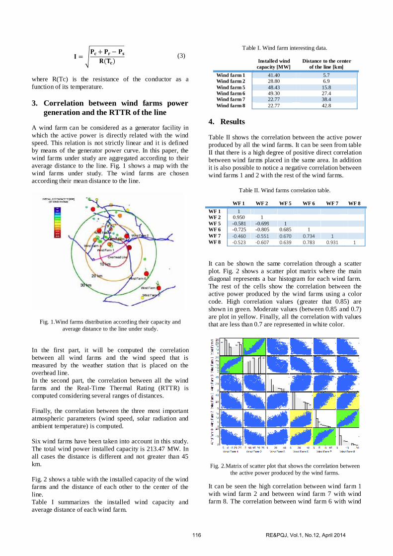
A wind farm can be considered as a generator facility in which the active power is directly related with the wind speed. This relation is not strictly linear and it is defined by means of the generator power curve. In this paper, the wind farms under study are aggregated according to their average distance to the line. Fig. 1 shows a map with the wind farms under study. The wind farms are chosen according their mean distance to the line.

Fig. 1.Wind farms distribution according their capacity and average distance to the line under study.

In the first part, it will be computed the correlation between all wind farms and the wind speed that is measured by the weather station that is placed on the overhead line. In the second part, the correlation between all the wind farms and the Real-Time Thermal Rating (RTTR) is computed considering several ranges of distances. Finally, the correlation between the three most important atmospheric parameters (wind speed, solar radiation and ambient temperature) is computed. Six wind farms have been taken into account in this study. The total wind power installed capacity is 213.47 MW. In all cases the distance is different and not greater than 45 km. Fig. 2 shows a table with the installed capacity of the wind farms and the distance of each other to the center of the line. Table I summarizes the installed wind capacity and average distance of each wind farm.

Table I. Wind farm interesting data.

Installed wind capacity [MW]

Distance to the center of the line [km]

Wind farm 1 41.40 5.7 Wind farm 2 28.80 6.9 Wind farm 5 48.43 15.8 Wind farm 6 49.30 27.4 Wind farm 7 22.77 38.4 Wind farm 8 22.77 42.8

4. Results Table II shows the correlation between the active power produced by all the wind farms. It can be seen from table II that there is a high degree of positive direct correlation between wind farms placed in the same area. In addition it is also possible to notice a negative correlation between wind farms 1 and 2 with the rest of the wind farms.

Table II. Wind farms correlation table.

WF 1 WF 2 WF 5 WF 6 WF 7 WF 8

WF 1 1 WF 2 0.950 1 WF 5 -0.581 -0.699 1 WF 6 -0.725 -0.805 0.685 1 WF 7 ‐0.460  ‐0.551  0.670  0.734  1   WF 8 ‐0.523  ‐0.607  0.639  0.783  0.931  1 

It can be shown the same correlation through a scatter plot. Fig. 2 shows a scatter plot matrix where the main diagonal represents a bar histogram for each wind farm. The rest of the cells show the correlation between the active power produced by the wind farms using a color code. High correlation values (greater that 0.85) are shown in green. Moderate values (between 0.85 and 0.7) are plot in yellow. Finally, all the correlation with values that are less than 0.7 are represented in white color.

Fig. 2.Matrix of scatter plot that shows the correlation between

the active power produced by the wind farms.

It can be seen the high correlation between wind farm 1 with wind farm 2 and between wind farm 7 with wind farm 8. The correlation between wind farm 6 with wind

116 RE&PQJ, Vol.1, No.12, April 2014

farm 7 and 8 is moderate and the rest of correlation values are lower than 0.75. Fig. 3 shows a scatter plot matrix where the main diagonal represents a bar histogram for the two variables, active power of all wind farms and the wind speed measured in the weather station placed in the overhead line. The two other cells show the correlation between the active power produced by the wind farms and the wind speed.

Fig. 3. Matrix of scatter plot that shows the correlation between

the power produced by all wind farms and the wind speed measured at weather station.

Fig. 4 shows the previous correlation between active power and wind speed more clearly.

Fig. 4. Linear fit of the active power of all wind farms and the wind speed measured at the weather station.

It can be observed that there is not a high correlation between all active power produced by the wind farms and the wind speed measured by the weather station.

Fig. 5 shows the correlation between the active power produced by a wind farm placed near (5.7 km) to the center of the overhead line and the wind measured in a weather station.

Fig. 5. Linear fit of the active power of wind farm 1 and the wind speed measured at the weather station.

The correlation between wind farm 1 and the wind speed measured in the weather station is negative. Fig. 6 shows the correlation between the active power produced by a wind farms placed a medium distance (15.8 km) to the center of the overhead line and the wind measured in a weather station.

Fig. 6. Linear fit of the active power of wind farm 5 and the wind speed measured at the weather station.

The correlation between wind farm 5 and the wind speed measured in the weather station is positive.

50 100 150P [MW] All W ind farms

0 5 10 15

40

60

80

100

120

140

Wind speed [m/s]

P [

MW

] A

ll W

ind

farm

s

0

5

10

15

Win

d sp

eed

[m/s

]

0 2 4 6 8 10 12 14 160

20

40

60

80

100

120

140

160

180

Wind speed [m/s]

P [

MW

] A

ll W

ind

farm

s

y = 0.7229*x + 66.9

0 2 4 6 8 10 12 14 160

5

10

15

20

25

30

35

Wind speed [m/s]

P [

MW

] W

ind

farm

1

y = - 1.756*x + 21.73

0 2 4 6 8 10 12 14 160

5

10

15

20

25

30

35

40

45

50

Wind speed [m/s]

P [

MW

] W

ind

farm

5

y = 1.38*x + 7.792

117 RE&PQJ, Vol.1, No.12, April 2014

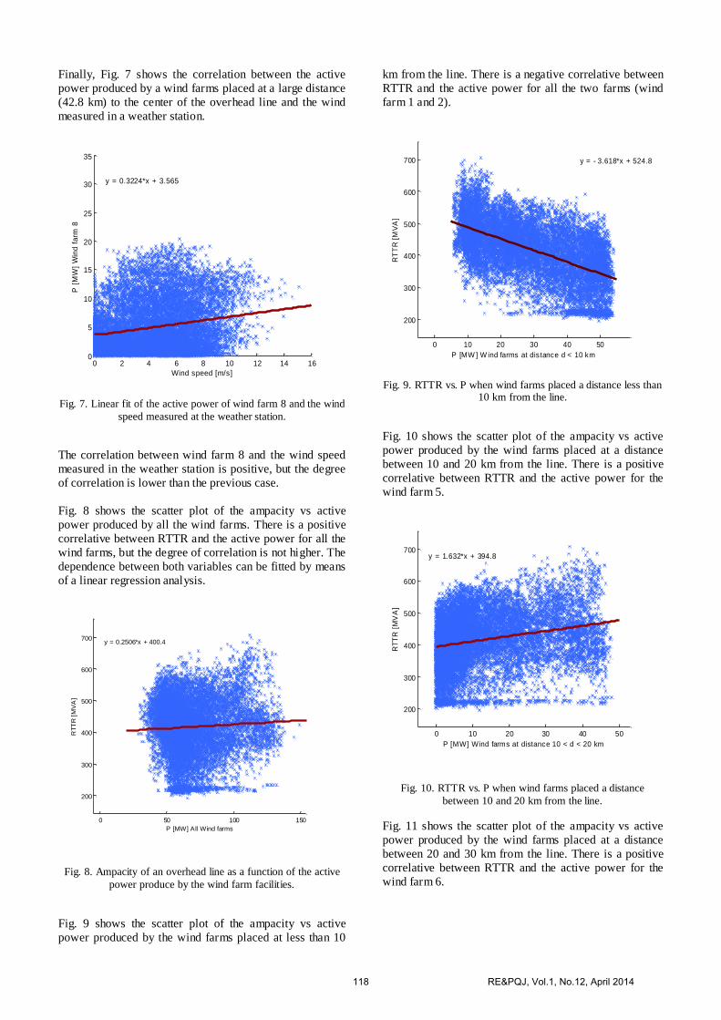
Finally, Fig. 7 shows the correlation between the active power produced by a wind farms placed at a large distance (42.8 km) to the center of the overhead line and the wind measured in a weather station.

Fig. 7. Linear fit of the active power of wind farm 8 and the wind

speed measured at the weather station.

The correlation between wind farm 8 and the wind speed measured in the weather station is positive, but the degree of correlation is lower than the previous case. Fig. 8 shows the scatter plot of the ampacity vs active power produced by all the wind farms. There is a positive correlative between RTTR and the active power for all the wind farms, but the degree of correlation is not higher. The dependence between both variables can be fitted by means of a linear regression analysis.

Fig. 8. Ampacity of an overhead line as a function of the active power produce by the wind farm facilities.

Fig. 9 shows the scatter plot of the ampacity vs active power produced by the wind farms placed at less than 10

km from the line. There is a negative correlative between RTTR and the active power for all the two farms (wind farm 1 and 2).

Fig. 9. RTTR vs. P when wind farms placed a distance less than

10 km from the line.

Fig. 10 shows the scatter plot of the ampacity vs active power produced by the wind farms placed at a distance between 10 and 20 km from the line. There is a positive correlative between RTTR and the active power for the wind farm 5.

Fig. 10. RTTR vs. P when wind farms placed a distance between 10 and 20 km from the line.

Fig. 11 shows the scatter plot of the ampacity vs active power produced by the wind farms placed at a distance between 20 and 30 km from the line. There is a positive correlative between RTTR and the active power for the wind farm 6.

0 2 4 6 8 10 12 14 160

5

10

15

20

25

30

35

Wind speed [m/s]

P [

MW

] W

ind

farm

8

y = 0.3224*x + 3.565

0 50 100 150

200

300

400

500

600

700

P [MW] All Wind farms

RT

TR

[M

VA

]

y = 0.2506*x + 400.4

0 10 20 30 40 50

200

300

400

500

600

700

P [MW ] W ind farms at distance d < 10 km

RT

TR

[M

VA

]

y = - 3.618*x + 524.8

0 10 20 30 40 50

200

300

400

500

600

700

P [MW] Wind farms at distance 10 < d < 20 km

RTT

R [

MV

A]

y = 1.632*x + 394.8

118 RE&PQJ, Vol.1, No.12, April 2014

Fig. 11. RTTR vs. P when wind farms placed a distance between

20 and 30 km from the line.

Fig. 12 shows the scatter plot of the ampacity vs active power produced by the wind farms placed at a distance greater than 30 km from the line. There is a positive correlative between RTTR and the active power for the two wind farms (wind farm 7 and 8).

Fig. 12. RTTR vs. P when wind farms placed a distance greater

than 30 km from the line.

Finally, Fig. 13 shows a scatter plot matrix where the main diagonal represents a bar histogram for three atmospheric variables, wind speed, solar irradiation and ambient temperature. All these variables are measured by the weather station. The rest of the cells represent the correlation between these variables. It is observed that there are a positive correlation between ambient temperature with wind speed and solar irradiation. The correlation between wind speed with solar irradiation is not clearly defined.

Fig. 13. Matrix of scatter plot that shows the correlation between the atmospheric variables.

5. Conclusions The correlation factor between the active power produced by a wind farm and the ampacity of the lines that are placed in the same geographical area shows a high degree of direct correlation. This correlation can be fit as a first-order polynomial and the error distribution can be computed as a way to know the degree of confidence of this approach.

Acknowledgement This work was supported by the Spanish Government under the R+D initiative INNPACTO with reference IPT-2011-1447-920000.

References [1] IEEE Standard for Calculating the Current-Temperature of Bare Overhead Conductors, IEEE Std 738-2006 (Revision of IEEE Std 738-1993). [2] Mathematical Model for Evaluation of Conductor Temperature in The Steady (or Quasi-Steady) State (Normal Operation),CIGRE, ELECTRA No. 144, Oct. 1992, pp. 109-115. [3] A. Madrazo, A. González, R. Martínez, M. Mañana, E. Hervás, A. Arroyo, P.B. Castro and D. Silió; Increasing Grid Integration of Wind Energy by using Ampacity Techniques. International Conference on Renewable Energies and Power Quality (ICREPQ’13). 2013. Bilbao.

0 10 20 30 40 50

200

300

400

500

600

700

P [MW] W ind farms at distance 20 < d < 30 km

RT

TR

[M

VA

]

y = 2.789*x + 367.7

0 10 20 30 40

200

300

400

500

600

700

P [MW] W ind farms at distance d > 30 km

RT

TR

[M

VA

]

y = 1.836*x + 402.3

0 10 20 30ambient temperature

0 500 1000solar radiation

0 5 10 150

10

20

30

wind speed

ambi

ent

tem

pera

ture

0

500

1000

sola

r ra

diat

ion

0

5

10

15

win

d sp

eed

119 RE&PQJ, Vol.1, No.12, April 2014