Hydrologic Data and Modeling: Towards Hydrologic Information Science
Indicators of Hydrologic Alteration
Version 7.1
withrPurview LLC - Ted Rybicki
Totten Software DesignSmythe Scientific Software
April 2009
User's Manual
Disclaimer: Because software is inherently complex and may not be completely free of errors, it is yourresponsibility to verify your work and make backup copies, and TNC will not be responsible for your failure to doso. In no event will TNC be liable for indirect, special, incidental, or consequential damages arising from use ofor inability to use this product, including, without limitation, damages or costs relating to the loss of profits,business goodwill, data or computer programs, even if advised of the possibility of such damages. The foregoinglimitations shall not apply to claims relating to death or personal injury which arise out of products deemed to beconsumer goods under applicable law. Some states do not allow the exclusion or limitation of implies warrantiesof limitation of liability for incidental or consequential damages, so the above exclusion or limitation may notapply to you.
Any commercial use of this software is prohibited without the express, written consent of TNC.
Citation for this document: The Nature Conservancy, 2009. Indicators of Hydrologic Alteration Version 7.1User's Manual.
Copyright © 1996-2009 The Nature Conservancy. All rights reserved. No part of thispublication or associated software may be reproduced or transmitted in any form or by anymeans, without prior written permission.
Indicators of Hydrologic Alteration
Version 7.1
User's Manual
IContents
Indicators of Hydrologic Alteration Version 7.1 help
Table of Contents
............................................................................................................................. 11. Introduction
.................................................................................................................................... 11.1 Welcome
.................................................................................................................................... 11.2 What's New in Version 7
.................................................................................................................................... 21.3 System Requirements
.................................................................................................................................... 31.4 Obtaining Hydrologic Data for Use in the IHA Software
............................................................................................................................. 52. Analyzing Hydrologic Data Using the IHA
.................................................................................................................................... 52.1 Introduction to Using the IHA
.................................................................................................................................... 62.2 IHA Parameters
.................................................................................................................................... 102.3 Environmental Flow Components
................................................................................................................................ 10Introduction to EFCs 2.3.1
................................................................................................................................ 12EFC Parameters 2.3.2
................................................................................................................................ 15EFC Calculation Algorithm 2.3.3
................................................................................................................................ 21Calibrating the EFC Algorithm 2.3.4
.................................................................................................................................... 222.4 RVA Analysis
.................................................................................................................................... 242.5 Flow Duration Curves
............................................................................................................................. 263. Setting Up and Running an IHA Analysis
.................................................................................................................................... 263.1 Introduction to Conducting an Analysis
.................................................................................................................................... 263.2 Importing Hydrologic Data
................................................................................................................................ 26Allowable Hydro Data Formats 3.2.1
................................................................................................................................ 28Importing and Editing Hydro Data Files 3.2.2
................................................................................................................................ 29Advice for Importing Particular Datasets 3.2.3
................................................................................................................................ 30Batch Import Capability 3.2.4
.................................................................................................................................... 313.3 Creating and Managing Projects
................................................................................................................................ 31Introduction to Projects 3.3.1
................................................................................................................................ 32Project Definition Tab 3.3.2
................................................................................................................................ 33Analysis List Tab 3.3.3
.................................................................................................................................... 333.4 Setting Up and Managing an Analysis
................................................................................................................................ 33Introduction to Analyses 3.4.1
................................................................................................................................ 35Analysis Title/Options Tab 3.4.2
................................................................................................................................ 35Analysis Years Tab 3.4.3
................................................................................................................................ 37Analysis Days Tab 3.4.4
................................................................................................................................ 38Statistics Tab 3.4.5
IHA Version 7.1 HelpII
Indicators of Hydrologic Alteration Version 7.1 help
................................................................................................................................ 39Environmental Flow Components Tab 3.4.6
................................................................................................................................ 40Flow Duration Curves Tab 3.4.7
.................................................................................................................................... 403.5 Running an Analysis
................................................................................................................................ 40Running an Analysis 3.5.1
................................................................................................................................ 41Batch Analysis 3.5.2
.................................................................................................................................... 443.6 Other Features
................................................................................................................................ 44Graph Default Settings 3.6.1
................................................................................................................................ 45Spreadsheet Tools 3.6.2
................................................................................................................................ 45Water Year Definition 3.6.3
................................................................................................................................ 47Working Directory 3.6.4
............................................................................................................................. 484. Viewing and Understanding IHA Outputs
.................................................................................................................................... 484.1 Introduction to Viewing Results
.................................................................................................................................... 484.2 Tables
................................................................................................................................ 48Introduction to Tables 4.2.1
................................................................................................................................ 50Annual Summaries Table 4.2.2
................................................................................................................................ 51Scorecard Table 4.2.3
................................................................................................................................ 53RVA Table 4.2.4
................................................................................................................................ 54Box-and-Whisker Table 4.2.5
................................................................................................................................ 54Regression Table 4.2.6
................................................................................................................................ 54Percentile Table 4.2.7
................................................................................................................................ 55EFC Daily Table 4.2.8
................................................................................................................................ 55Flow Duration Curve Table 4.2.9
................................................................................................................................ 55Message Report 4.2.10
.................................................................................................................................... 554.3 Graphs
................................................................................................................................ 55Introduction to Graphs 4.3.1
................................................................................................................................ 56Summary of IHA Graphs 4.3.2
................................................................................................................................ 57Editing and Working with IHA Graphs 4.3.3
................................................................................................................................ 59Chart Editor 4.3.4
............................................................................................................................. 615. Technical Notes
.................................................................................................................................... 615.1 Introduction to Technical Notes
.................................................................................................................................... 615.2 Empirical Percentiles
.................................................................................................................................... 615.3 Julian Dates and Statistics for Timing Variables
.................................................................................................................................... 645.4 Missing Data and Data Interpolation
.................................................................................................................................... 655.5 Shortened Water Years and Seasons
.................................................................................................................................... 665.6 Maximum Number of Years of Hydrologic Data
.................................................................................................................................... 665.7 Metadata for an IHA Analysis
.................................................................................................................................... 705.8 Issues with Large Flow Values
IIIContents
Indicators of Hydrologic Alteration Version 7.1 help
.................................................................................................................................... 705.9 Warning Messages
.................................................................................................................................... 725.10 Bug-Tracking Feature
.................................................................................................................................... 735.11 Regional and Language Settings
.................................................................................................................................... 735.12 DOS Command Line Start-Up
............................................................................................................................. 746. Endnotes
IHA Version 7.1 Help1
Indicators of Hydrologic Alteration Version 7.1 help
1 Introduction
1.1 Welcome
Welcome to the rapidly growing community of Indicators of Hydrologic Alteration (IHA)software users! This software has been developed by The Nature Conservancy (TNC) as aneasy-to-use tool for calculating the characteristics of natural and altered hydrologic regimes. The method and software will work on any type of daily hydrologic data, such as streamflows,river stages, ground water levels, or lake levels. The power of the IHA method is that it can beused to summarize long periods of daily hydrologic data into a much more manageable series ofecologically relevant hydrologic parameters.
The main IHA webpage is: http://conserveonline.org/workspaces/iha.
The scientific basis behind the software and some sample applications are described in Richteret al. (1996, 1997, 1998), which are available on the website. Note that the definition of someof the parameters and the methods for calculating them has changed since these papers werepublished. Additionally, TNC maintains a database of IHA users, which describes manydifferent applications of the software. The database is also available on the website. Lastly,the website now has additional training resources on the IHA, including an on-line course inEnglish and Spanish.
We hope that you will find these methods useful for understanding and managing changes inhydrologic systems.
For those using the IHA for the first time, a basic tutorial is available. The tutorial document isavailable on your program menu once the software is installed, and is also located in the IHAinstallation directory (default is c:\Program files\IHAV7).
1.2 What's New in Version 7
Version 7 of the IHA has some significant improvements from earlier versions. The mostimportant new features are:
(1) A new and improved interface, with enhanced spreadsheet and graphing tools for viewingIHA results. Results tables can now be viewed and edited in spreadsheet format, and savedas Excel spreadsheets. A new graphing package has also been incorporated into the IHA toprovide users with the capability to create publication quality graphs inside the IHA.
(2) The ability to import flow data in three different formats. Data can be imported directlyfrom files downloaded from the U.S. Geological Survey website, from a generic two columntext file format, and from .dat files created by the data import utility in Version 6 of the IHA.
(3) Many of the calculations have been revamped to improve the consistency between how
different flow parameters are calculated, and also to improve the non-parametric nature ofsome of the statistical calculations. See Analyzing Hydrologic Data Using the IHA and also
Introduction 2
Indicators of Hydrologic Alteration Version 7.1 help
the Technical Notes for details on how different calculations are done. Be aware that thesechanges mean that some parameter values will be different than those computed by earlierversions of the software. In particular, the values in the Annual Summaries Table for non-parametric analysis are now medians of the relevant sub-annual data, whereas in earlierversions of the software, these values were means.
(4) An improved help system, with context-sensitive help. To get help from within theprogram, click on Help | IHA Help, hit the available Help button, or hit F1 on yourkeyboard. A basic tutorial on how to use the software is also included. The tutorialdocument is available on your program menu once the software is installed, and is alsolocated in the IHA installation directory (default is c:\Program files\IHAV7).
(5) Environmental Flow Components (EFCs). This is a large new suite of hydrologic flowparameters, which represent an attempt to automatically identify and compute statistics onhydrological events such as floods and droughts. EFCs were actually initiated in Version 6of the software, but are mentioned here because that version was not widely distributed. For a further description of EFCs, see EFC Parameters.
Version 7.1 also has the following additional features:
(1) The ability to compare two different flow datasets. This gives users the ability to compareflows from two different stream gauges or from two different model runs or scenarios. Thecomputations are identical to a comparison of two different periods in a single flow dataset.See Introduction to Projects and Project Definition Tab for more information on this option.
(2) The EFC algorithm has been improved to simplify the default version of the algorithm, andalso to provide greater flexibility in calibration. See EFC Calculation Algorithm andCalibrating the EFC Algorithm for description of these features.
(3) Flow duration curves (FDCs) have been added to the IHA. IHA will compute FDCs usingthe same periods, years, and days used for the 33 IHA statistics. FDC results are displayedin a new tab on the results spreadsheet, and are computed annually and for each month. It ispossible to view any number of FDCs on the same graph. See Flow Duration Curves formore information.
(4) Spanish language user manual and help system.
(5) Note that while Version 7.1 of the IHA will open projects created in Version 7, once that isdone, it will no longer be possible to use those projects with Version 7, since somealterations will be made in the IHA data files.
1.3 System Requirements
The program has been tested and will run reliably under the Windows 98, ME, NT, 2000, XP,and Vista Operating Systems. Brief tests indicate that it will not work reliably under Windows95.
IHA Version 7.1 Help3
Indicators of Hydrologic Alteration Version 7.1 help
The installation will require approximately 6 MB of disk space. The calculations require verylittle computing power, but the graphics will have satisfactory performance only on Pentium 3and faster processors.
1.4 Obtaining Hydrologic Data for Use in the IHA Software
The IHA software uses daily data for its calculations. The IHA statistics will be meaningfulonly when calculated for a sufficiently long hydrologic record. The length of record necessaryto obtain reliable pre- vs. post-impact comparisons (with minimal influence of climaticvariation) is a matter of current research. Presently, we are recommending that at least twentyyears of daily records be used for each pre-impact and post-impact period, as well as for trendanalysis. This is based on Richter et al. (1997), who found that for three different types ofstreams in the United States, measures of the central tendency or dispersion of annual 1-daymaximum flows converged around the long-term mean when at least 20 years of data wereused.
Some other recent articles on the issue of how many years of data are necessary to obtainreliable results are Taylor et al. (2003) and Huh et al. (2005). When Taylor et al.(unpublished) tested the impact of different record lengths on IHA output statistics for a highlyvariable South African river, they found that for some IHA parameters 20 years was sufficientto account for natural climatic variability, but for others 35 or more years of data were needed.More data was needed for more variable parameters and for extreme events such as largefloods. In sum, while 20 years should be considered a good baseline requirement for theamount of data needed, the number of years of data needed may vary depending on the (1)degree of climate variability; (2) the frequency or variability of the particular parameter; (3)the severity of the hydrologic alteration that you are trying to detect; (4) and whether the goal isto characterize the central tendency or range of inter-annual variability (it seems to take lessdata to adequately characterize changes in the central tendency). If there is doubt about howmuch data is enough, some tests to see how different record lengths affect IHA statistics wouldbe prudent.
Richter et al. (1997) also discuss various methods for extending hydrologic records, filling inmissing data, or estimating daily hydrologic data from simulation modeling.
The IHA automatically does linear interpolation over gaps in the data; therefore, users shouldregard any IHA results from datasets with missing records with appropriate caution!
Hydrologic data can usually be obtained directly from the agency or organization that collectsthe data. In the United States, the vast majority of streamflow data are collected by the U.S.Geological Survey (USGS). Their data archive is conveniently available on the internet at http://water.usgs.gov/usa/nwis. Daily streamflow data downloaded from this website can beimported directly into the IHA.
Other federal agencies within the U.S., such as the U.S. Forest Service or U.S. Bureau of LandManagement, also collect streamflow data on some of the streams located on lands they
Introduction 4
Indicators of Hydrologic Alteration Version 7.1 help
manage. Some lake level and ground water well data are also available from the USGS, butmuch of this type of data is collected and managed by other local governmental entities. Usually, a few phone calls to local water departments or natural resource departments willlead you to the appropriate source of the data you are seeking, if it exists.
Private vendors, such as Hydrosphere Data (http://www.hydrosphere.com) have compiledUSGS data onto CD-ROM disks, which are available for an annual subscription fee.
Daily flow data from the Water Survey of Canada are available on the internet at http://www.wsc.ec.gc.ca/hydat/H2O/.
Finally, the IHA can also be run using daily flow data generated by a hydrologic model or othersimulation method.
While the IHA is primarily designed for analyzing streamflow data expressed in units of flow(cubic feet per second or cubic meters per second), there is no reason why data in differentunits or groundwater and lake levels expressed as elevations could not be also used in the IHA.
See Allowable Data Formats for more information on data import formats and requirements.
IHA Version 7.1 Help5
Indicators of Hydrologic Alteration Version 7.1 help
2 Analyzing Hydrologic Data Using the IHA
2.1 Introduction to Using the IHA
The IHA will calculate a total of 67 statistical parameters. These parameters are subdividedinto 2 groups, the IHA parameters and the Environmental Flow Component (EFC) parameters. There are 33 IHA Parameters and 34 EFC Parameters. This software has many options whichcan be used to control how these parameters are calculated, which are described briefly in thissection. The output tables and graphs produced by the IHA will vary depending on whichoptions are used (see Viewing and Understanding IHA Outputs for more description).
An important choice that will have to be made is whether to compare two distinct time periodsor analyze trends over a single time period. If the hydrologic system you wish to study hasexperienced an abrupt change such as construction of a dam, the IHA can be used to analyzehow the flow regime was affected by computing the hydrologic parameters for two timeperiods, before and after the impact. For hydrologic systems that have experienced a long-termaccumulation of human modifications, the IHA can compute and graph linear regressions toevaluate the trend. As of Version 7.1, it is also possible to compare two different flowdatasets. The computations and outputs here are identical to those from a two period analysis,except that two different flow datasets are being compared, as opposed to two different periodsin a single flow dataset. See Setting Up and Managing an Analysis for information on how toset the time periods for these various types of analyses, and Tables for how output tables differdepending on the type of analysis being conducted.
IHA parameters can be calculated using parametric (mean/standard deviation) or non-parametric (percentile) statistics. For most situations non-parametric statistics are a betterchoice, because of the skewed (non-normal) nature of many hydrologic datasets (a keyassumption of parametric statistics is that the data are normally distributed). But for certainsituations, such as flood frequency or average monthly flow volumes, parametric statistics maybe preferable. See Setting Up and Managing An Analysis for information on how to specifynon-parametric vs. parametric analysis. See IHA Parameters and EFC Parameters for morespecifics on how calculations will vary for parametric versus non-parametric analysis, and see Tables and Graphs for details on how output tables and graphs will differ.
The hydrologic parameters produced by the IHA are calculated and organized in the outputtables by water year. The default water year in the IHA is Oct. 1 - Sept. 30, but the water yearcan be reset to start on any other day of the year (see Water Year Definition for more details).Certain parameters can also be calculated for periods shorter than an entire year (see ShortenedWater Years and Seasons). IHA parameters can be calculated for a shortened part of the wateryear, and EFC parameters other than monthly low flows may be calculated separately for twodifferent seasons, each of which covers only a part of the water year.
When analyzing the change between two time periods, the software enables users to implementthe Range of Variability Approach (RVA) described in Richter et al. (1997). See RVAAnalysis for further description. Note that RVA Analysis is only available for IHA parameters,not for the EFC parameters.
Analyzing Hydrologic Data Using the IHA 6
Indicators of Hydrologic Alteration Version 7.1 help
As of version 7.1, the IHA can also compute Flow Curation Curves (FDCs). FDCs arecomputed for all data, and separately for each month, using the same time periods, years, andshortened water years that are used for the other statistics. One additional option is that FDCscan be computed for only selected years in each period. See the section on Flow DurationCurves for more details.
2.2 IHA Parameters
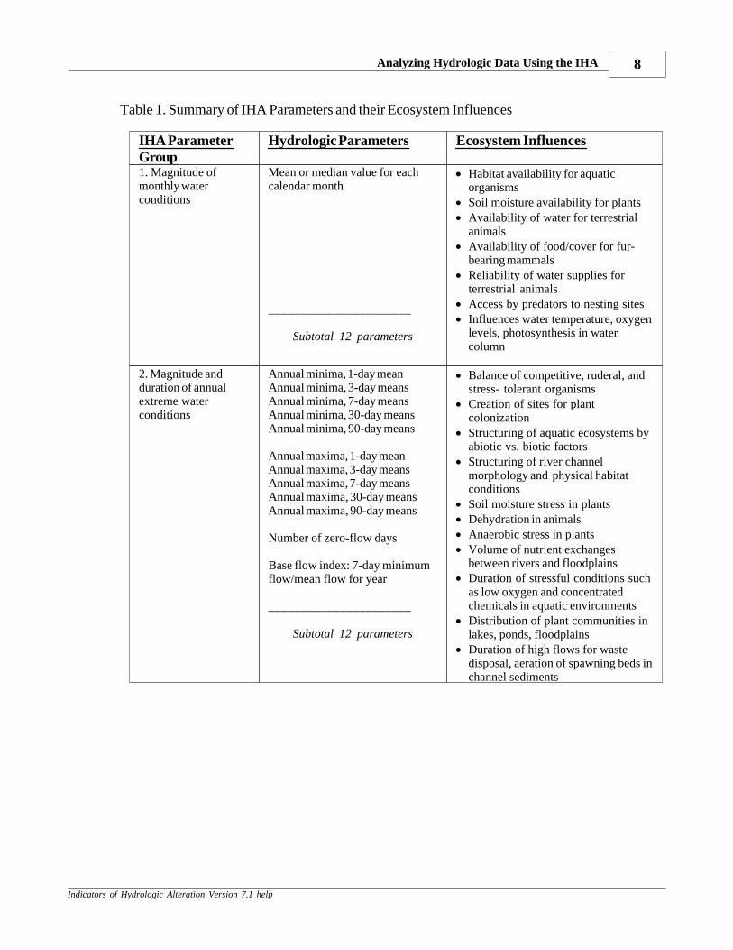
The 33 IHA parameters are described in Table 1 (see the following page), along with theirecosystem influences. Whether a mean or median value is calculated depends on whether theuser has selected parametric or non-parametric analysis. Note that moving averages (1-day to30-day minimums and maximums) are always calculated as means.
Some important notes regarding the calculation of IHA parameters are as follows:
· When using a shortened water year, IHA parameters are calculated using only the data in theshortened period. Monthly average flows that overlap the boundary of the shortened periodwill be calculated only for the portion of the month that is in the period. For directions onhow to set a shortened water year, see Setting Up and Managing an Analysis.
· For parameter group 2 (extreme water conditions), the 3-, 7-, 30-, and 90-day minimums andmaximums are taken from moving averages of the appropriate length calculated for everypossible period that is completely within the water year.
· The zero-flow days and base flow index parameters in group 2 are modeled after the suite offlow parameters described by Poff and Ward (1989).
· For parameter group 3 (extreme water conditions), if there are multiple days in the wateryear with the same flow value, the earliest date is reported.
· For parameter group 4 (high and low pulses), a day is classified as a pulse if it is greaterthan or less than a specified threshold, which can be set by the user (see Setting Up andManaging an Analysis). For two period analysis pulse thresholds are calculated using datain the pre-impact period only, while for single period analysis pulse thresholds arecalculated using data from the entire period. If a shortened water year is used, the pulsethresholds are computed using data within the shortened water year only. Periods of dayswhich are in the same type of pulse are counted as a distinct pulse event. High and low pulseevents that overlap between water years are counted only in the water year in which theybegin, and the duration of these events includes the part that occurs in the subsequent wateryear. Similarly, in cases where a shortened water year is used, only events that start in thatshortened water year are included in the statistics, but the entire length of the event is used,even if it ends outside the shortened water year. In some cases a missing water year of dataor the end of the dataset may truncate a pulse that is counted in the statistics. When thishappens, a warning is issued in the Message Report, so that the user knows that one event hasa truncated duration. Note that events that start on the first day of the dataset or the first dayafter a missing water year are not counted in the statistics, because it is assumed that these
IHA Version 7.1 Help7
Indicators of Hydrologic Alteration Version 7.1 help
events actually began in the prior water year that is not in the data.
· Reversals (in parameter group 5) are calculated by dividing the hydrologic record into"rising" and "falling" periods, which correspond to periods in which daily changes in flowsare either positive or negative, respectively. Note that a rising or falling period is not endedby a pair of days with constant flow, only by a change of sign in the rate of change. Thenumber of reversals is the number of times that flow switches from one type of period toanother. Reversals are analyzed on a water year by water year basis, so the first change inflow of the water year cannot be counted as a reversal, since no rising or falling trend existsbefore then.
Analyzing Hydrologic Data Using the IHA 8
Indicators of Hydrologic Alteration Version 7.1 help
Table 1. Summary of IHA Parameters and their Ecosystem Influences
IHA ParameterGroup
Hydrologic Parameters Ecosystem Influences
1. Magnitude ofmonthly waterconditions
Mean or median value for eachcalendar month
______________________
Subtotal 12 parameters
· Habitat availability for aquaticorganisms
· Soil moisture availability for plants· Availability of water for terrestrial
animals· Availability of food/cover for fur-
bearing mammals· Reliability of water supplies for
terrestrial animals· Access by predators to nesting sites · Influences water temperature, oxygen
levels, photosynthesis in watercolumn
2. Magnitude andduration of annualextreme waterconditions
Annual minima, 1-day meanAnnual minima, 3-day meansAnnual minima, 7-day meansAnnual minima, 30-day meansAnnual minima, 90-day means
Annual maxima, 1-day meanAnnual maxima, 3-day meansAnnual maxima, 7-day meansAnnual maxima, 30-day meansAnnual maxima, 90-day means
Number of zero-flow days
Base flow index: 7-day minimumflow/mean flow for year
______________________
Subtotal 12 parameters
· Balance of competitive, ruderal, andstress- tolerant organisms
· Creation of sites for plantcolonization
· Structuring of aquatic ecosystems byabiotic vs. biotic factors
· Structuring of river channelmorphology and physical habitatconditions
· Soil moisture stress in plants· Dehydration in animals· Anaerobic stress in plants· Volume of nutrient exchanges
between rivers and floodplains· Duration of stressful conditions such
as low oxygen and concentrated chemicals in aquatic environments
· Distribution of plant communities inlakes, ponds, floodplains
· Duration of high flows for wastedisposal, aeration of spawning beds inchannel sediments
IHA Version 7.1 Help9
Indicators of Hydrologic Alteration Version 7.1 help
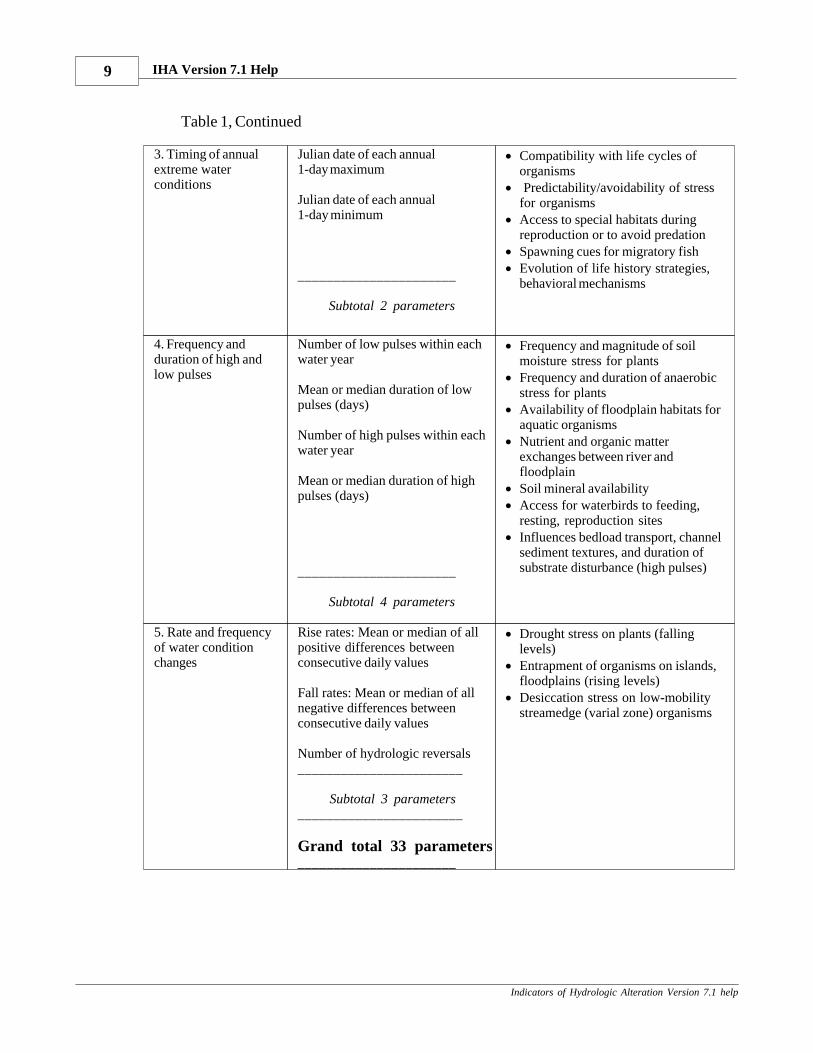
Table 1, Continued
3. Timing of annualextreme waterconditions
Julian date of each annual 1-day maximum
Julian date of each annual 1-day minimum
______________________
Subtotal 2 parameters
· Compatibility with life cycles oforganisms
· Predictability/avoidability of stressfor organisms
· Access to special habitats duringreproduction or to avoid predation
· Spawning cues for migratory fish· Evolution of life history strategies,
behavioral mechanisms
4. Frequency andduration of high andlow pulses
Number of low pulses within eachwater year
Mean or median duration of lowpulses (days)
Number of high pulses within eachwater year
Mean or median duration of highpulses (days)
______________________
Subtotal 4 parameters
· Frequency and magnitude of soilmoisture stress for plants
· Frequency and duration of anaerobicstress for plants
· Availability of floodplain habitats foraquatic organisms
· Nutrient and organic matterexchanges between river andfloodplain
· Soil mineral availability · Access for waterbirds to feeding,
resting, reproduction sites · Influences bedload transport, channel
sediment textures, and duration ofsubstrate disturbance (high pulses)
5. Rate and frequencyof water conditionchanges
Rise rates: Mean or median of allpositive differences betweenconsecutive daily values
Fall rates: Mean or median of allnegative differences betweenconsecutive daily values
Number of hydrologic reversals_______________________
Subtotal 3 parameters_______________________
Grand total 33 parameters______________________
· Drought stress on plants (fallinglevels)
· Entrapment of organisms on islands,floodplains (rising levels)
· Desiccation stress on low-mobilitystreamedge (varial zone) organisms
Analyzing Hydrologic Data Using the IHA 10
Indicators of Hydrologic Alteration Version 7.1 help
2.3 Environmental Flow Components
2.3.1 Introduction to EFCs
The IHA calculates parameters for five different types of Environment Flow Components(EFCs): low flows, extreme low flows, high flow pulses, small floods, and large floods. Thisdelineation of EFCs is based on the realization by research ecologists that river hydrographscan be divided into a repeating set of hydrographic patterns that are ecologically relevant. It isthe full spectrum of flow conditions represented by these five types of flow events that must bemaintained in order to sustain riverine ecological integrity. Not only is it essential to maintainadequate flows during low flow periods, but higher flows and floods and also extreme lowflow conditions also perform important ecological functions. For more on EFCs, see EFCParameters and EFC Calculation Algorithm. The five EFC types are described in more detailbelow.
Low flows – This is the dominant flow condition in most rivers. In natural rivers, after arainfall event or snowmelt period has passed and associated surface runoff from the catchmenthas subsided, the river returns to its base- or low-flow level. These low-flow levels aresustained by groundwater discharge into the river. The seasonally-varying low-flow levels ina river impose a fundamental constraint on a river's aquatic communities because it determinesthe amount of aquatic habitat available for most of the year. This has a strong influence on thediversity and number of organisms that can live in the river.
Extreme low flows – During drought periods, rivers drop to very low levels that can bestressful for many organisms, but may provide necessary conditions for other species. Waterchemistry, temperature, and dissolved oxygen availability can become highly stressful to manyorganisms during extreme low flows, to the point that these conditions can cause considerablemortality. On the other hand, extreme low flows may concentrate aquatic prey for somespecies, or may be necessary to dry out low-lying floodplain areas and enable certain speciesof plants such as bald cypress to regenerate.
High-flow pulses – During rainstorms or brief periods of snowmelt, a river will rise above itslow-flow level. As defined here, high-flow pulses include any water rises that do not overtopthe channel banks. These pulses provide important and necessary disruptions in low flows. Even a small or brief flush of fresh water can provide much-needed relief from higher watertemperatures or low oxygen conditions that typify low-flow periods, and deliver a nourishingsubsidy of organic material or other food to support the aquatic food web. High-flow pulsesalso provide fish and other mobile creatures with increased access to up- and downstreamareas.
Small floods – During floods, fish and other mobile organisms are able to move upstream,downstream, and out into floodplains or flooded wetlands to access additional habitats such assecondary channels, backwaters, sloughs, and shallow flooded areas. These usuallyinaccessible areas can provide substantial food resources. Shallow flooded areas are typicallywarmer than the main channel and full of nutrients and insects that fuel rapid growth in aquaticorganisms. As used here, a "small flood" includes all river rises that overtop the main channelbut does not include more extreme, and less frequent, floods.
IHA Version 7.1 Help11
Indicators of Hydrologic Alteration Version 7.1 help
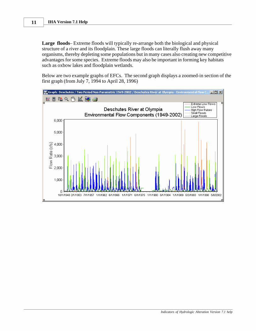
Large floods – Extreme floods will typically re-arrange both the biological and physicalstructure of a river and its floodplain. These large floods can literally flush away manyorganisms, thereby depleting some populations but in many cases also creating new competitiveadvantages for some species. Extreme floods may also be important in forming key habitatssuch as oxbow lakes and floodplain wetlands.
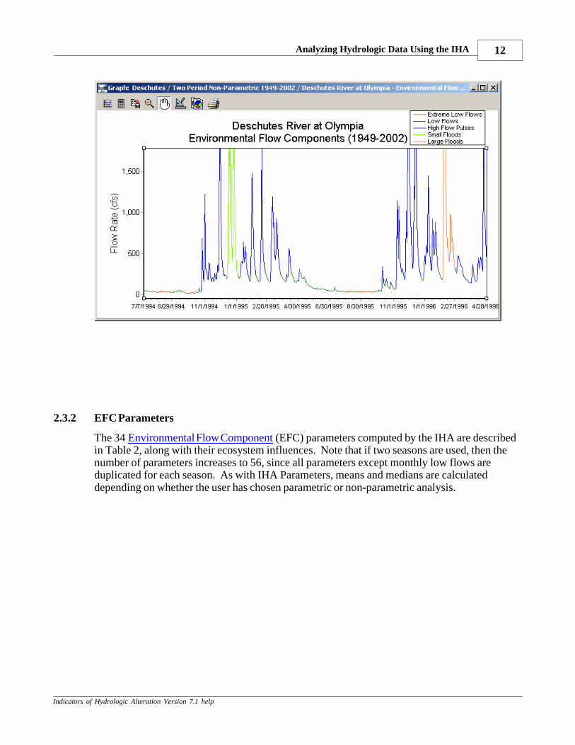
Below are two example graphs of EFCs. The second graph displays a zoomed-in section of thefirst graph (from July 7, 1994 to April 28, 1996)
Analyzing Hydrologic Data Using the IHA 12
Indicators of Hydrologic Alteration Version 7.1 help
2.3.2 EFC Parameters
The 34 Environmental Flow Component (EFC) parameters computed by the IHA are describedin Table 2, along with their ecosystem influences. Note that if two seasons are used, then thenumber of parameters increases to 56, since all parameters except monthly low flows areduplicated for each season. As with IHA Parameters, means and medians are calculateddepending on whether the user has chosen parametric or non-parametric analysis.
IHA Version 7.1 Help13
Indicators of Hydrologic Alteration Version 7.1 help
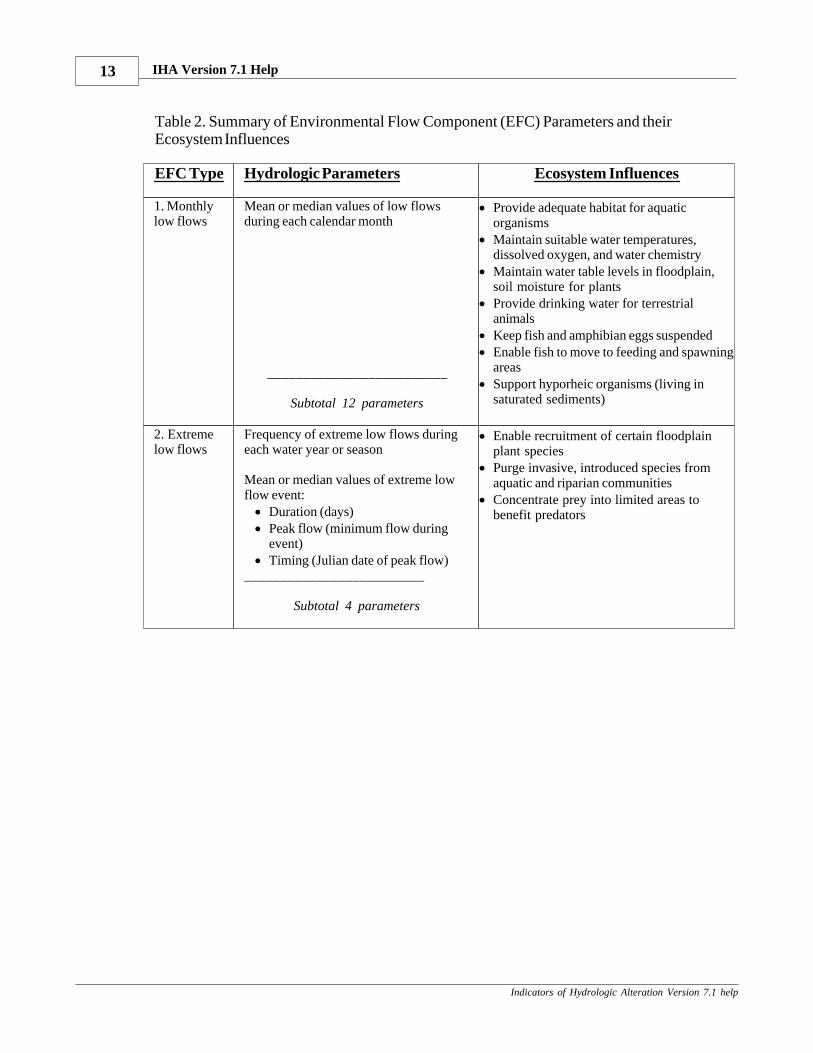
Table 2. Summary of Environmental Flow Component (EFC) Parameters and theirEcosystem Influences
EFC Type Hydrologic Parameters Ecosystem Influences
1. Monthlylow flows
Mean or median values of low flowsduring each calendar month
_________________________
Subtotal 12 parameters
· Provide adequate habitat for aquaticorganisms
· Maintain suitable water temperatures,dissolved oxygen, and water chemistry
· Maintain water table levels in floodplain,soil moisture for plants
· Provide drinking water for terrestrialanimals
· Keep fish and amphibian eggs suspended· Enable fish to move to feeding and spawning
areas· Support hyporheic organisms (living in
saturated sediments)
2. Extremelow flows
Frequency of extreme low flows duringeach water year or season
Mean or median values of extreme lowflow event:
· Duration (days)· Peak flow (minimum flow during
event)· Timing (Julian date of peak flow)
_________________________
Subtotal 4 parameters
· Enable recruitment of certain floodplainplant species
· Purge invasive, introduced species fromaquatic and riparian communities
· Concentrate prey into limited areas tobenefit predators
Analyzing Hydrologic Data Using the IHA 14
Indicators of Hydrologic Alteration Version 7.1 help
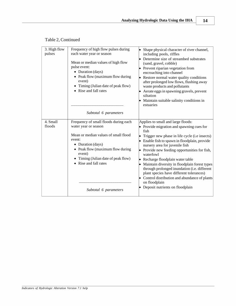
Table 2, Continued
3. High flowpulses
Frequency of high flow pulses duringeach water year or season
Mean or median values of high flowpulse event:
· Duration (days)· Peak flow (maximum flow during
event)· Timing (Julian date of peak flow)· Rise and fall rates
_________________________
Subtotal 6 parameters
· Shape physical character of river channel,including pools, riffles
· Determine size of streambed substrates(sand, gravel, cobble)
· Prevent riparian vegetation fromencroaching into channel
· Restore normal water quality conditionsafter prolonged low flows, flushing awaywaste products and pollutants
· Aerate eggs in spawning gravels, preventsiltation
· Maintain suitable salinity conditions inestuaries
4. Smallfloods
Frequency of small floods during eachwater year or season
Mean or median values of small floodevent:
· Duration (days)· Peak flow (maximum flow during
event)· Timing (Julian date of peak flow)· Rise and fall rates
_________________________
Subtotal 6 parameters
Applies to small and large floods:· Provide migration and spawning cues for
fish· Trigger new phase in life cycle (i.e insects)· Enable fish to spawn in floodplain, provide
nursery area for juvenile fish· Provide new feeding opportunities for fish,
waterfowl· Recharge floodplain water table· Maintain diversity in floodplain forest types
through prolonged inundation (i.e. differentplant species have different tolerances)
· Control distribution and abundance of plantson floodplain
· Deposit nutrients on floodplain
IHA Version 7.1 Help15
Indicators of Hydrologic Alteration Version 7.1 help
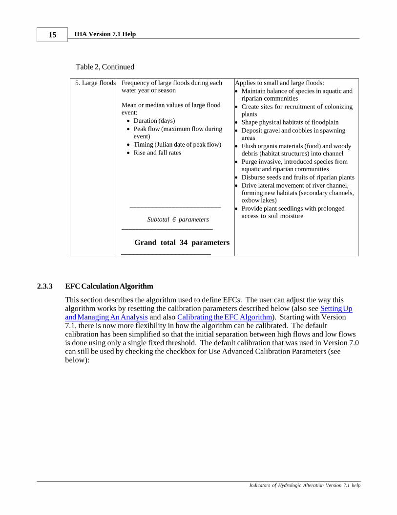
Table 2, Continued
5. Large floods Frequency of large floods during eachwater year or season
Mean or median values of large floodevent:
· Duration (days)· Peak flow (maximum flow during
event)· Timing (Julian date of peak flow)· Rise and fall rates
__________________________
Subtotal 6 parameters__________________________
Grand total 34 parameters_______________________
Applies to small and large floods:· Maintain balance of species in aquatic and
riparian communities· Create sites for recruitment of colonizing
plants· Shape physical habitats of floodplain· Deposit gravel and cobbles in spawning
areas· Flush organis materials (food) and woody
debris (habitat structures) into channel· Purge invasive, introduced species from
aquatic and riparian communities· Disburse seeds and fruits of riparian plants· Drive lateral movement of river channel,
forming new habitats (secondary channels,oxbow lakes)
· Provide plant seedlings with prolongedaccess to soil moisture
2.3.3 EFC Calculation Algorithm
This section describes the algorithm used to define EFCs. The user can adjust the way thisalgorithm works by resetting the calibration parameters described below (also see Setting Upand Managing An Analysis and also Calibrating the EFC Algorithm). Starting with Version7.1, there is now more flexibility in how the algorithm can be calibrated. The defaultcalibration has been simplified so that the initial separation between high flows and low flowsis done using only a single fixed threshold. The default calibration that was used in Version 7.0can still be used by checking the checkbox for Use Advanced Calibration Parameters (seebelow):
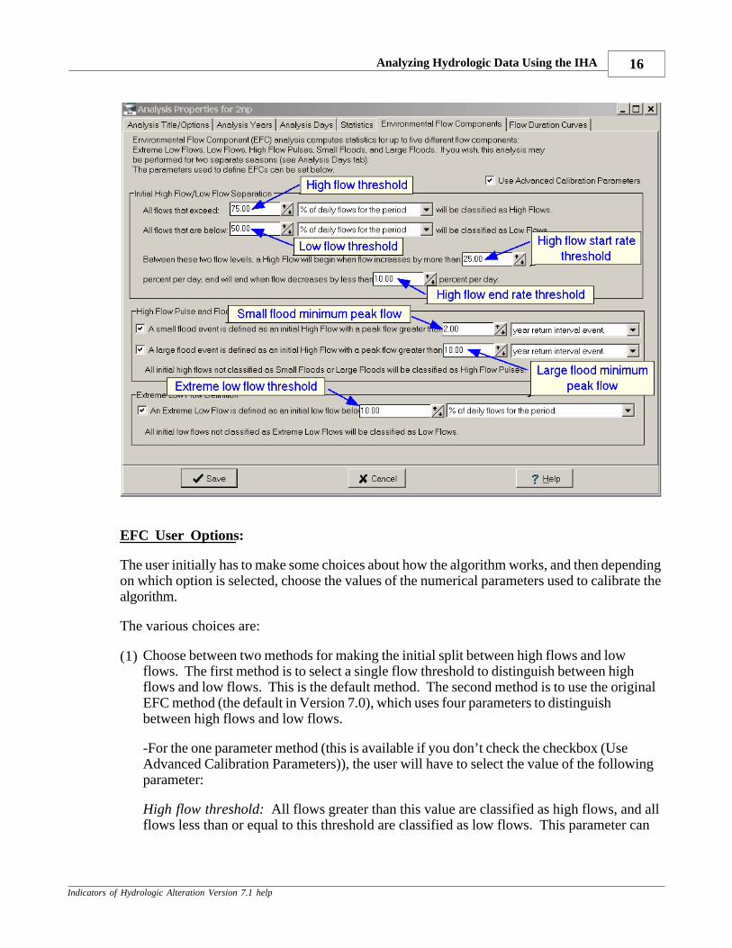
Analyzing Hydrologic Data Using the IHA 16
Indicators of Hydrologic Alteration Version 7.1 help
EFC User Options:
The user initially has to make some choices about how the algorithm works, and then dependingon which option is selected, choose the values of the numerical parameters used to calibrate thealgorithm.
The various choices are:
(1) Choose between two methods for making the initial split between high flows and lowflows. The first method is to select a single flow threshold to distinguish between highflows and low flows. This is the default method. The second method is to use the originalEFC method (the default in Version 7.0), which uses four parameters to distinguishbetween high flows and low flows.
-For the one parameter method (this is available if you don’t check the checkbox (UseAdvanced Calibration Parameters)), the user will have to select the value of the followingparameter:
High flow threshold: All flows greater than this value are classified as high flows, and allflows less than or equal to this threshold are classified as low flows. This parameter can
IHA Version 7.1 Help17
Indicators of Hydrologic Alteration Version 7.1 help
be specified as a percentile of all daily flows or as a flow value. The default value is the75th percentile of daily flows.
-For the four parameter method (this is available if you check the checkbox (Use AdvancedCalibration Parameters)), the user will have to select the values of the followingparameters:
High flow threshold: All flows greater than this threshold are classified as high flows.This parameter can be specified as a percentile of all daily flows or as a flow value. Thedefault value is the 75th percentile of daily flows.
Low flow threshold: All flows less than or equal to this threshold are classified as lowflow events. This parameter must always be less than the high flow threshold. Thisparameter can be specified as a percentile of all daily flows or as a flow value. Thedefault value is the 50th percentile of daily flows.
High flow start rate threshold: When flows are between the high flow and low flowthresholds, this parameter controls the start of high flow events. It also controls whetherthe ascending limb of an event is restarted from the descending limb. The default value is25%.
High flow end rate threshold: When flows are between the high flow and low flowthresholds, this parameter is used to end high flow events during their descending limb. Italso controls the transition between the ascending and descending limb of an event. Thedefault value is 10%.
(2) Choose the number of high flow classes to specify, using the appropriate checkboxes. Thiscan be 1, 2, or 3. If there is one class it will be called high flow pulses. If there are twoclasses they will be called high flow pulses and either small floods or large floods (theuser’s choice). If there are 3 classes they will be called high flow pulses, small floods,and large floods.
For 2 or 3 classes, the user must specify one or both of the following 2 parameters:
Small flood minimum peak flow: All high flow events that have a peak flow greater thanor equal to this value (and less than the peak flow value for large floods, if there are 3 flowclasses) will be assigned to the small flood class. All events with a peak flow less thanthis value will be assigned to the high flow pulse class. The user has the option to enterthis as either a return interval, a flow value, or a percentile of all daily flows. The defaultvalue is the 2 year return interval.
Large flood minimum peak flow: All high flow events that have a peak flow greater thanor equal to this value will be assigned to the large flood class. All events with a peak flowless than this value will be assigned to the high flow pulse class or the small flood class,depending on whether there are 2 or 3 high flow classes. The user has the option to enterthis as either a return interval, a flow value, or a percentile of all daily flows. The defaultvalue is the 10 year return interval.
Analyzing Hydrologic Data Using the IHA 18
Indicators of Hydrologic Alteration Version 7.1 help
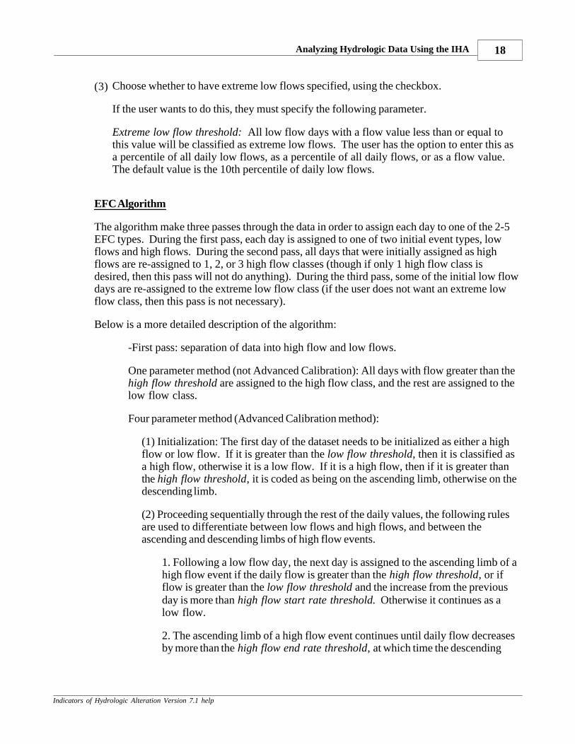
(3) Choose whether to have extreme low flows specified, using the checkbox.
If the user wants to do this, they must specify the following parameter.
Extreme low flow threshold: All low flow days with a flow value less than or equal tothis value will be classified as extreme low flows. The user has the option to enter this asa percentile of all daily low flows, as a percentile of all daily flows, or as a flow value. The default value is the 10th percentile of daily low flows.
EFC Algorithm
The algorithm make three passes through the data in order to assign each day to one of the 2-5EFC types. During the first pass, each day is assigned to one of two initial event types, lowflows and high flows. During the second pass, all days that were initially assigned as highflows are re-assigned to 1, 2, or 3 high flow classes (though if only 1 high flow class isdesired, then this pass will not do anything). During the third pass, some of the initial low flowdays are re-assigned to the extreme low flow class (if the user does not want an extreme lowflow class, then this pass is not necessary).
Below is a more detailed description of the algorithm:
-First pass: separation of data into high flow and low flows.
One parameter method (not Advanced Calibration): All days with flow greater than the high flow threshold are assigned to the high flow class, and the rest are assigned to thelow flow class.
Four parameter method (Advanced Calibration method):
(1) Initialization: The first day of the dataset needs to be initialized as either a highflow or low flow. If it is greater than the low flow threshold, then it is classified asa high flow, otherwise it is a low flow. If it is a high flow, then if it is greater thanthe high flow threshold, it is coded as being on the ascending limb, otherwise on thedescending limb.
(2) Proceeding sequentially through the rest of the daily values, the following rulesare used to differentiate between low flows and high flows, and between theascending and descending limbs of high flow events.
1. Following a low flow day, the next day is assigned to the ascending limb of ahigh flow event if the daily flow is greater than the high flow threshold, or ifflow is greater than the low flow threshold and the increase from the previousday is more than high flow start rate threshold. Otherwise it continues as alow flow.
2. The ascending limb of a high flow event continues until daily flow decreasesby more than the high flow end rate threshold, at which time the descending
IHA Version 7.1 Help19
Indicators of Hydrologic Alteration Version 7.1 help
limb of the event is started.
3. During the descending limb of a high flow event, the ascending limb isrestarted if daily flow increases by more than the high flow start rate threshold.
4. During the descending limb of a high flow event, the event is ended if the rateof decrease of flow drops below the high flow end rate threshold (meaning thatthe change in flow is between -1 * high flow end rate threshold and high flowstart rate threshold), unless the flow is still greater than or equal to the highflow threshold, in which case the descending limb continues.
5. The event is always ended if flow drops down to equal to or below the lowflow threshold, regardless of whether the event is on the ascending ordescending limb.
6. After the high flow is ended, a low flow condition resumes.
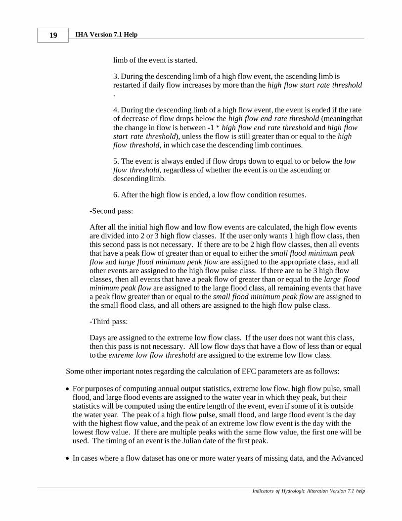
-Second pass:
After all the initial high flow and low flow events are calculated, the high flow eventsare divided into 2 or 3 high flow classes. If the user only wants 1 high flow class, thenthis second pass is not necessary. If there are to be 2 high flow classes, then all eventsthat have a peak flow of greater than or equal to either the small flood minimum peakflow and large flood minimum peak flow are assigned to the appropriate class, and allother events are assigned to the high flow pulse class. If there are to be 3 high flowclasses, then all events that have a peak flow of greater than or equal to the large floodminimum peak flow are assigned to the large flood class, all remaining events that havea peak flow greater than or equal to the small flood minimum peak flow are assigned tothe small flood class, and all others are assigned to the high flow pulse class.
-Third pass:
Days are assigned to the extreme low flow class. If the user does not want this class,then this pass is not necessary. All low flow days that have a flow of less than or equalto the extreme low flow threshold are assigned to the extreme low flow class.
Some other important notes regarding the calculation of EFC parameters are as follows:
· For purposes of computing annual output statistics, extreme low flow, high flow pulse, smallflood, and large flood events are assigned to the water year in which they peak, but theirstatistics will be computed using the entire length of the event, even if some of it is outsidethe water year. The peak of a high flow pulse, small flood, and large flood event is the daywith the highest flow value, and the peak of an extreme low flow event is the day with thelowest flow value. If there are multiple peaks with the same flow value, the first one will beused. The timing of an event is the Julian date of the first peak.
· In cases where a flow dataset has one or more water years of missing data, and the Advanced
Analyzing Hydrologic Data Using the IHA 20
Indicators of Hydrologic Alteration Version 7.1 help
Calibration method is being used, the initialization procedure described above is rerun aftereach period of missing data. Note also that the occurrence of missing water years of datameans that some EFC events may be truncated either at their beginning or end. Ourconvention is to count any events in the statistics that are truncated by the end of a water year,but ignore events that are truncated by the beginning of a water year. In either of thesesituations, a warning is issued in the Message Report. Be aware that the truncated events thatare counted may have errors in flow parameters such as peak flow, duration, timing, and riseand fall rates, due to the fact that not all of the event is present in the flow data. Also, in therare case that the peak of a high flow event occurs on the last day before a missing year, nofall rate from that event is used to compute annual statistics, since it cannot be calculated.
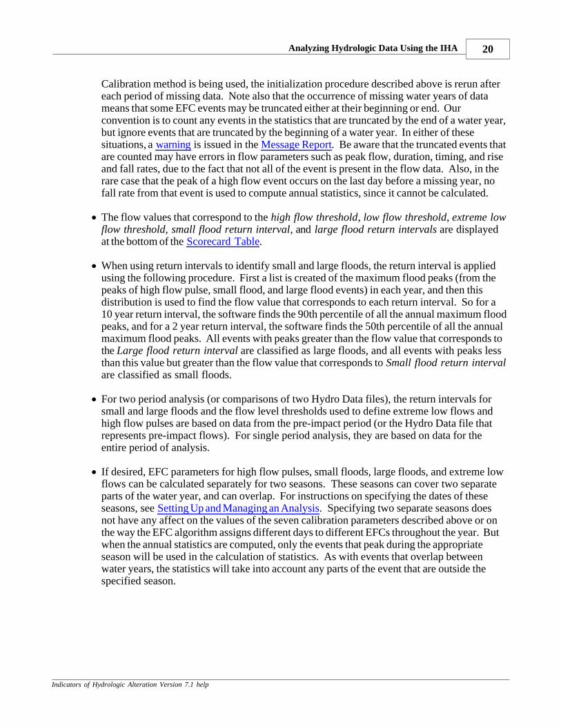
· The flow values that correspond to the high flow threshold, low flow threshold, extreme lowflow threshold, small flood return interval, and large flood return intervals are displayedat the bottom of the Scorecard Table.
· When using return intervals to identify small and large floods, the return interval is appliedusing the following procedure. First a list is created of the maximum flood peaks (from thepeaks of high flow pulse, small flood, and large flood events) in each year, and then thisdistribution is used to find the flow value that corresponds to each return interval. So for a10 year return interval, the software finds the 90th percentile of all the annual maximum floodpeaks, and for a 2 year return interval, the software finds the 50th percentile of all the annualmaximum flood peaks. All events with peaks greater than the flow value that corresponds tothe Large flood return interval are classified as large floods, and all events with peaks lessthan this value but greater than the flow value that corresponds to Small flood return intervalare classified as small floods.
· For two period analysis (or comparisons of two Hydro Data files), the return intervals forsmall and large floods and the flow level thresholds used to define extreme low flows andhigh flow pulses are based on data from the pre-impact period (or the Hydro Data file thatrepresents pre-impact flows). For single period analysis, they are based on data for theentire period of analysis.
· If desired, EFC parameters for high flow pulses, small floods, large floods, and extreme lowflows can be calculated separately for two seasons. These seasons can cover two separateparts of the water year, and can overlap. For instructions on specifying the dates of theseseasons, see Setting Up and Managing an Analysis. Specifying two separate seasons doesnot have any affect on the values of the seven calibration parameters described above or onthe way the EFC algorithm assigns different days to different EFCs throughout the year. Butwhen the annual statistics are computed, only the events that peak during the appropriateseason will be used in the calculation of statistics. As with events that overlap betweenwater years, the statistics will take into account any parts of the event that are outside thespecified season.
IHA Version 7.1 Help21
Indicators of Hydrologic Alteration Version 7.1 help
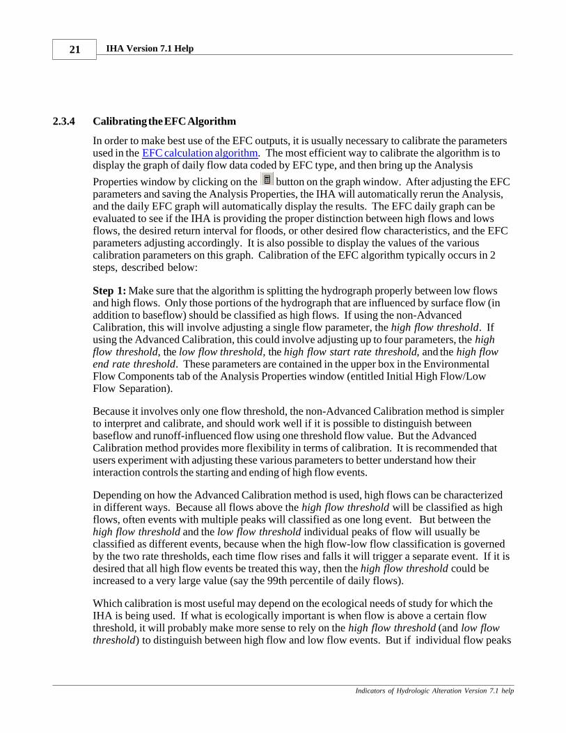
2.3.4 Calibrating the EFC Algorithm
In order to make best use of the EFC outputs, it is usually necessary to calibrate the parametersused in the EFC calculation algorithm. The most efficient way to calibrate the algorithm is todisplay the graph of daily flow data coded by EFC type, and then bring up the Analysis
Properties window by clicking on the button on the graph window. After adjusting the EFCparameters and saving the Analysis Properties, the IHA will automatically rerun the Analysis,and the daily EFC graph will automatically display the results. The EFC daily graph can beevaluated to see if the IHA is providing the proper distinction between high flows and lowsflows, the desired return interval for floods, or other desired flow characteristics, and the EFCparameters adjusting accordingly. It is also possible to display the values of the variouscalibration parameters on this graph. Calibration of the EFC algorithm typically occurs in 2steps, described below:
Step 1: Make sure that the algorithm is splitting the hydrograph properly between low flowsand high flows. Only those portions of the hydrograph that are influenced by surface flow (inaddition to baseflow) should be classified as high flows. If using the non-AdvancedCalibration, this will involve adjusting a single flow parameter, the high flow threshold. Ifusing the Advanced Calibration, this could involve adjusting up to four parameters, the highflow threshold, the low flow threshold, the high flow start rate threshold, and the high flowend rate threshold. These parameters are contained in the upper box in the EnvironmentalFlow Components tab of the Analysis Properties window (entitled Initial High Flow/LowFlow Separation).
Because it involves only one flow threshold, the non-Advanced Calibration method is simplerto interpret and calibrate, and should work well if it is possible to distinguish betweenbaseflow and runoff-influenced flow using one threshold flow value. But the AdvancedCalibration method provides more flexibility in terms of calibration. It is recommended thatusers experiment with adjusting these various parameters to better understand how theirinteraction controls the starting and ending of high flow events.
Depending on how the Advanced Calibration method is used, high flows can be characterizedin different ways. Because all flows above the high flow threshold will be classified as highflows, often events with multiple peaks will classified as one long event. But between the high flow threshold and the low flow threshold individual peaks of flow will usually beclassified as different events, because when the high flow-low flow classification is governedby the two rate thresholds, each time flow rises and falls it will trigger a separate event. If it isdesired that all high flow events be treated this way, then the high flow threshold could beincreased to a very large value (say the 99th percentile of daily flows).
Which calibration is most useful may depend on the ecological needs of study for which theIHA is being used. If what is ecologically important is when flow is above a certain flowthreshold, it will probably make more sense to rely on the high flow threshold (and low flowthreshold) to distinguish between high flow and low flow events. But if individual flow peaks

Analyzing Hydrologic Data Using the IHA 22
Indicators of Hydrologic Alteration Version 7.1 help
are better treated as individual events because each peak has some ecological significance,then the second method described in the previous paragraph may be better.
Step 2: Once the hydrograph has been properly split between high flows and low flows, thenext step is to calibrate the separation of high flows into high flow pulses, small floods, andlarge floods, and the separation of the low flows into low flows and extreme low flows. Thiscalibration can be done specifying whether 1, 2 or 3 high flow classes are desired, whetherextreme low flows are desired, and by adjusting the small flood and large flood minimum peakflows and extreme low flow threshold. These parameters are contained in the bottom twoboxes of the Environmental Flow Components tab of the Analysis Properties window.
Since floods are typically defined as events that overtop the main channel and extend into thefloodplain, data on the flow rate that causes such behavior would be useful in calibrating thereturn interval thresholds. Another type of information that could be useful in calibrationwould be the flood flow rates that are necessary to perform specific ecological functions. Sothe EFC algorithm could be calibrated to generate statistics on floods that are necessary forcottonwood recruitment, that promote fish spawning, or that perform other functions. Similarphysical and ecological considerations could be used to calibrate the extreme low flows.
2.4 RVA Analysis
When analyzing the change between two time periods (or comparing two Hydro Data files), theIHA software enables users to implement the Range of Variability Approach (RVA) describedin Richter et al. (1997). The RVA uses the pre-development natural variation of IHAparameter values as a reference for defining the extent to which natural flow regimes have beenaltered. The pre-development variation can also be used as a basis for defining initialenvironmental flow goals. Richter et al (1997) suggest that water managers should strive tokeep the distribution of annual values of the IHA parameters as close to the pre-impactdistributions as possible. RVA analysis also generates a series of Hydrologic Alterationfactors, which quantify the degree of alteration of the 33 IHA flow parameters. Note that RVAanalysis is only available for IHA parameters, and not for EFC parameters.
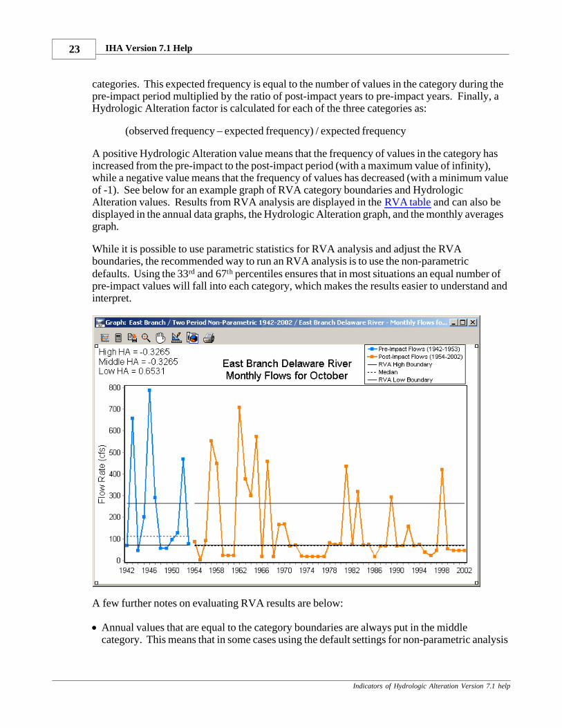
In an RVA analysis, the full range of pre-impact data for each parameter is divided into threedifferent categories. The boundaries between categories are based on either percentile values(for non-parametric analysis) or a number of standard deviations away from the mean (forparametric analysis), which are specified by the user (see Setting Up and Managing an Analysis). As an example, the default in non-parametric RVA analysis is to place the categoryboundaries 17 percentiles from the median. This yields an automatic delineation of threecategories of equal size: the lowest category contains all values less than or equal to the 33rd
percentile; the middle category contains all values falling in the range of the 34th to 67th
percentiles; and the highest category contains all values greater than the 67th percentile.
The program then computes the expected frequency with which the "post-impact" values of theIHA parameters should fall within each category (in the non-parametric default, this would be33% for each of the three categories). The program then computes the frequency with whichthe "post-impact" annual values of IHA parameters actually fell within each of the three
IHA Version 7.1 Help23
Indicators of Hydrologic Alteration Version 7.1 help
categories. This expected frequency is equal to the number of values in the category during thepre-impact period multiplied by the ratio of post-impact years to pre-impact years. Finally, aHydrologic Alteration factor is calculated for each of the three categories as:
(observed frequency – expected frequency) / expected frequency
A positive Hydrologic Alteration value means that the frequency of values in the category hasincreased from the pre-impact to the post-impact period (with a maximum value of infinity),while a negative value means that the frequency of values has decreased (with a minimum valueof -1). See below for an example graph of RVA category boundaries and HydrologicAlteration values. Results from RVA analysis are displayed in the RVA table and can also bedisplayed in the annual data graphs, the Hydrologic Alteration graph, and the monthly averagesgraph.
While it is possible to use parametric statistics for RVA analysis and adjust the RVAboundaries, the recommended way to run an RVA analysis is to use the non-parametricdefaults. Using the 33rd and 67th percentiles ensures that in most situations an equal number ofpre-impact values will fall into each category, which makes the results easier to understand andinterpret.
A few further notes on evaluating RVA results are below:
· Annual values that are equal to the category boundaries are always put in the middlecategory. This means that in some cases using the default settings for non-parametric analysis
Analyzing Hydrologic Data Using the IHA 24
Indicators of Hydrologic Alteration Version 7.1 help
will not always yield an equal distribution of annual values between the three categories. Insome cases it may be possible to adjust the RVA boundaries to get a more even distributionbetween categories, but in some cases uneven distributions may be unavoidable.
· The RVA method may also yield non-intuitive results for parameters which have a largenumber of annual statistics equal to a particular value. For example, the number of zero flowdays often has many of its annual values equal to 0, which can mean that both the 33rd and the67th percentile are also equal to 0.
· There are a few situations where it is impossible to calculate RVA boundaries and/orHydrologic Alteration factors. If there is one year of pre-impact data or no years of post-impact data, RVA boundaries are not calculated, so in the RVA table these rows along withthe expected and observed frequencies and Hydrologic Alteration factors will be blank. When this happens, a notice is put in the Message Report listing the parameters for which thisis the case. Also, if the denominator in the equation for Hydrologic Alteration (expectedfrequency) is equal to 0, the Hydrologic Alteration factor is reported as a blank in the RVATable, to avoid a divide by zero error.
· There are two IHA parameters which may not have annual values in all years (low pulse andhigh pulse durations). For these parameters, the HA values will affected not only by therelative distribution of annual values between the three categories, but also by the change inthe frequency of events from the pre-impact to the post-impact period. If the frequency ofpulse events is greatly reduced from the pre-impact to the post-impact period, it will bepossible to get a negative HA for all three categories, a result which should not occur for anyother parameters.
For all of these reasons, RVA results should be scrutinized carefully, and different methods forspecifying RVA boundaries may need to be tried to get useful results. Problems such as thesecan usually be diagnosed by examining the category boundaries in the RVA table and also theannual values in the Annual Summaries table.
2.5 Flow Duration Curves
The IHA will compute Flow Duration Curves (FDCs) separately for each period of analysis(for single and two period analyses) or for each Hydro Data file (for projects that compare twodifferent Hydro Data files). The exact periods, years, and days of data used in thesecomputations are determined by the same settings used to specify years of analysis and days ofanalysis for the 33 IHA parameters (on the Analysis Years tab and the Analysis Days tab). Inaddition, for the FDCs only, the user can use only selected years of data in each period orHydro Data file being analyzed. This selection can be done on the Flow Duration Curves tab.Using data from the periods, years, days selected, FDCs will be computed using all theavailable data (this is called the annual FDC). Also, separate FDCs will be computed for eachmonth, though to simplify the computations, these computations ignore the settings on the

IHA Version 7.1 Help25
Indicators of Hydrologic Alteration Version 7.1 help
Analysis Days tab (but use the settings on the Analysis Years tab and the Flow DurationCurves tab)
FDCs are computed using the following method:
Step 1: Sort (rank) average daily discharges for period of record from the largest value tothe smallest value, involving a total of n values.
Step 2: Assign each discharge value a rank (M), starting with 1 for the largest dailydischarge value.
Step 3: Calculate exceedence probability (P) as follows:
P = 100 * [ M / (n + 1) ]
P = the probability that a given flow will be equaled or exceeded (% of time) M = the ranked position on the listing (dimensionless) n = the number of events for period of record (dimensionless)
FDC results are then shown in the Flow Duration Curve Table, with flow values (ranked fromhighest to lowest) and exceedance probabilities for the annual and each monthly FDC. Resultscan also be displayed graphically (see below for an example graph). Any selection of annualand monthly FDCs can be displayed on the same graph.
Setting Up and Running an IHA Analysis 26
Indicators of Hydrologic Alteration Version 7.1 help
3 Setting Up and Running an IHA Analysis
3.1 Introduction to Conducting an Analysis
Setting up and completing an analysis in the IHA involves the following steps:
(1) Importing hydrologic data. Data can be imported from three different file formats, and thensaved as an internal Hydrologic Data file.
(2) Creating a Project. Each Project is linked to a single Hydrologic Data file, and can beused to create and run multiple Analyses.
(3) Creating and setting up an Analysis. Each Analysis stores a series of user-settableparameters that define how the hydrologic data will be analyzed. Multiple Analyses can besaved in a single Project.
(4) Running an Analysis.
(5) Viewing results. Results are available in table and graph format.
The IHA contains a self-explanatory Wizard to guide you through all these steps. The first timethe software is run, the user will have then option of starting the Wizard from the welcomepage. It can also be accessed by clicking IHA | Wizard.
3.2 Importing Hydrologic Data
3.2.1 Allowable Hydro Data Formats
The IHA can import daily hydrologic data from three different text file formats:
(1)Daily streamflow data downloaded from the U.S. Geological Survey (USGS) website.These data are available at http://nwis.waterdata.usgs.gov/nwis/sw (click on the link forDaily Data), and can be downloaded as a text file with tab-separated values. The IHAwill import data that has any of the available date formats. Note that during the summer of2006, the USGS changed the format of data available at this website. The IHA will importeither the old or the new format. But be aware that while the new format files may containdata other than daily mean discharge, the IHA will only import mean daily discharge datain cubic feet per second (cfs) from these data files, and nothing else. In some cases it ispossible to download multiple columns for one station that have mean daily discharge datain cfs. In these cases, the IHA will import the cfs column that is farthest to the right in thefile. USGS discharge data for the current water year will usually be provisional, whichmeans that it has not been finalized for publication and could be revised in the future. TheIHA will issue a warning if such data exists in the file.
(2)Data in the .dat file format used by earlier versions of the IHA. This data consists of a
IHA Version 7.1 Help27
Indicators of Hydrologic Alteration Version 7.1 help
column of data for each water year, with 367 rows in each column. The first row containsthe year, and the rest of the rows contain the flow values for each day (or 999999 for dayswith missing data), in order. The columns can be delimited by a space or a comma, andmust be terminated by an end-of-line character. The years must continue in increasingorder from left to right, although it is acceptable to have some missing years.
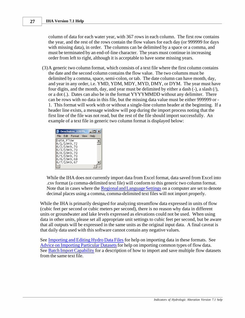
(3)A generic two column format, which consists of a text file where the first column containsthe date and the second column contains the flow value. The two columns must bedelimited by a comma, space, semi-colon, or tab. The date column can have month, day,and year in any order, i.e. YMD, YDM, MDY, MYD, DMY, or DYM. The year must havefour digits, and the month, day, and year must be delimited by either a dash (-), a slash (/),or a dot (.). Dates can also be in the format YYYYMMDD without any delimiter. Therecan be rows with no data in this file, but the missing data value must be either 999999 or -1. This format will work with or without a single-line column header at the beginning. If aheader line exists, a message window will pop during the import process noting that thefirst line of the file was not read, but the rest of the file should import successfully. Anexample of a text file in generic two column format is displayed below:
While the IHA does not currently import data from Excel format, data saved from Excel into.csv format (a comma-delimited text file) will conform to this generic two column format. Note that in cases where the Regional and Language Settings on a computer are set to denotedecimal places using a comma, comma-delimited text files will not import properly.
While the IHA is primarily designed for analyzing streamflow data expressed in units of flow(cubic feet per second or cubic meters per second), there is no reason why data in differentunits or groundwater and lake levels expressed as elevations could not be used. When usingdata in other units, please set all appropriate unit settings to cubic feet per second, but be awarethat all outputs will be expressed in the same units as the original input data. A final caveat isthat daily data used with this software cannot contain any negative values.
See Importing and Editing Hydro Data Files for help on importing data in these formats. SeeAdvice on Importing Particular Datasets for help on importing common types of flow data.See Batch Import Capability for a description of how to import and save multiple flow datasetsfrom the same text file.
Setting Up and Running an IHA Analysis 28
Indicators of Hydrologic Alteration Version 7.1 help
3.2.2 Importing and Editing Hydro Data Files
To import data into the IHA, click IHA | Hydrologic Data | Import Data File. Once pointedtowards a file, the IHA will automatically determine which of the three allowable file types thedata correspond to, and then proceed to import the data. If batch processing is necessary, thatwill also be determined automatically (see Batch Import Capability for a description of howthis works). For data in .dat file format and generic two column format, the user will beprompted to specify some additional information about the file. For data in .dat file format, theuser will need to specify the date of the first flow value in the file. For data in generic twocolumn format, the user will need to specify if a no data value is used in the file (and what thatvalue is) and also the units of flow (cubic feet per second or cubic meters per second). Fordata in USGS file format and .dat file format, flow data is assumed to be cubic feet per second,because those are the usual units in which these data are distributed.
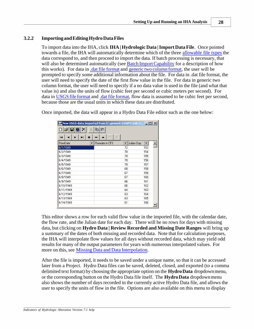
Once imported, the data will appear in a Hydro Data File editor such as the one below:
This editor shows a row for each valid flow value in the imported file, with the calendar date,the flow rate, and the Julian date for each day. There will be no rows for days with missingdata, but clicking on Hydro Data | Review Recorded and Missing Date Ranges will bring upa summary of the dates of both missing and recorded data. Note that for calculation purposes,the IHA will interpolate flow values for all days without recorded data, which may yield oddresults for many of the output parameters for years with numerous interpolated values. Formore on this, see Missing Data and Data Interpolation.
After the file is imported, it needs to be saved under a unique name, so that it can be accessedlater from a Project. Hydro Data files can be saved, deleted, closed, and exported (to a commadelimited text format) by choosing the appropriate option on the Hydro Data dropdown menu,or the corresponding button on the Hydro Data file itself. The Hydro Data dropdown menualso shows the number of days recorded in the currently active Hydro Data file, and allows theuser to specify the units of flow in the file. Options are also available on this menu to display
IHA Version 7.1 Help29
Indicators of Hydrologic Alteration Version 7.1 help
Projects that are related to the current Hydro Data file, start a new Project with the currentHydro Data file, and close all Project, graph, and table windows related to the Hydro Data file.
Records can be added to and deleted from the Hydro Data file in the editor window, and thevalues in the file can also be edited. Any changes that are made to file must be saved ordiscarded before leaving the Hydro Data editor. Clicking on the column headers will sort therecords, and clicking on the triangle to the right of the column header will bring up a customauto filter which can be used to filter out some records from view. These last two options arefor viewing purposes only, and do not affected the saved file.
To re-open an existing Hydro Data file, click on IHA | Hydrologic Data | Open Existing File.
The IHA can process up to 500 years of hydrologic data (see Maximum Numbers of Years inHydrologic Data).
3.2.3 Advice for Importing Particular Datasets
This section provides step-by-step procedures for converting common types of daily flow datainto formats that can be imported directly into the IHA.
Army Corps of Engineers HEC-DSS database files
This conversion procedure uses the HEC-DSS MS Excel add-in tool to extract data from .dssfiles. This add-in is available on the HEC website: http://www.hec.usace.army.mil/. Note thatonly daily data can be imported into the IHA (.dss files may hold other types of data).
(1) Open the .dss file using the Excel add-in tool.(2) Retrieve regular time series by selection.(3) In the catalog, set the date range to the range you wish to import, and import the desireddata into Excel.(4) Once the data is imported into the spreadsheet, delete the header information above theflow data, and the left (empty) column.(5) Save the data out of Excel as a .csv text file.(6) Import the .csv file into the IHA.
If there are negative values in the data, the IHA will ignore these when doing the import. Assuming that these values represent days with missing data, converting them to a -1 or a999999 will make the import cleaner (these are the no data values accepted by the IHA). But itwill work either way.
Water Survey of Canada data
These data are available in the internet at http://www.wsc.ec.gc.ca/hydat/H2O/. Thisconversion procedure is for data in the following file format: DATE-DATE FORMAT (CSV). The file should contain only one type of data (flow or stage), so that there is no duplication ofcalendar dates in the file.
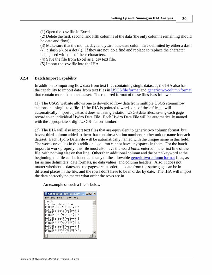
Setting Up and Running an IHA Analysis 30
Indicators of Hydrologic Alteration Version 7.1 help
(1) Open the .csv file in Excel.(2) Delete the first, second, and fifth columns of the data (the only columns remaining shouldbe date and flow).(3) Make sure that the month, day, and year in the date column are delimited by either a dash(-), a slash (/), or a dot (.). If they are not, do a find and replace to replace the characterbeing used with one of these characters. (4) Save the file from Excel as a .csv text file.(5) Import the .csv file into the IHA.
3.2.4 Batch Import Capability
In addition to importing flow data from text files containing single datasets, the IHA also hasthe capability to import data from text files in USGS file format and generic two column formatthat contain more than one dataset. The required format of these files is as follows:
(1) The USGS website allows one to download flow data from multiple USGS streamflowstations in a single text file. If the IHA is pointed towards one of these files, it willautomatically import it just as it does with single station USGS data files, saving each gagerecord to an individual Hydro Data File. Each Hydro Data File will be automatically namedwith the appropriate 8-digit USGS station number.
(2) The IHA will also import text files that are equivalent to generic two column format, buthave a third column added to them that contains a station number or other unique name for eachdataset. Each Hydro Data File will be automatically named with the unique name in this field. The words or values in this additional column cannot have any spaces in them. For the batchimport to work properly, this file must also have the word batch entered in the first line of thefile, with nothing else on that line. Other than additional column and the batch keyword at thebeginning, the file can be identical to any of the allowable generic two column format files, asfar as line delimiters, date formats, no data values, and column headers. Also, it does notmatter whether the dates and the gages are in order, i.e. data from the same gage can be indifferent places in the file, and the rows don't have to be in order by date. The IHA will importthe data correctly no matter what order the rows are in.
An example of such a file is below:
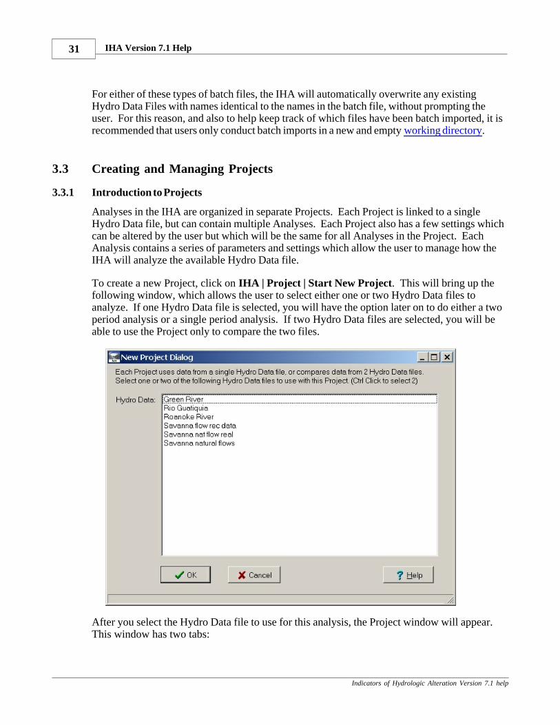
IHA Version 7.1 Help31
Indicators of Hydrologic Alteration Version 7.1 help
For either of these types of batch files, the IHA will automatically overwrite any existingHydro Data Files with names identical to the names in the batch file, without prompting theuser. For this reason, and also to help keep track of which files have been batch imported, it isrecommended that users only conduct batch imports in a new and empty working directory.
3.3 Creating and Managing Projects
3.3.1 Introduction to Projects
Analyses in the IHA are organized in separate Projects. Each Project is linked to a singleHydro Data file, but can contain multiple Analyses. Each Project also has a few settings whichcan be altered by the user but which will be the same for all Analyses in the Project. EachAnalysis contains a series of parameters and settings which allow the user to manage how theIHA will analyze the available Hydro Data file.
To create a new Project, click on IHA | Project | Start New Project. This will bring up thefollowing window, which allows the user to select either one or two Hydro Data files toanalyze. If one Hydro Data file is selected, you will have the option later on to do either a twoperiod analysis or a single period analysis. If two Hydro Data files are selected, you will beable to use the Project only to compare the two files.
After you select the Hydro Data file to use for this analysis, the Project window will appear. This window has two tabs:
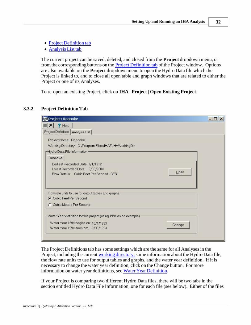
Setting Up and Running an IHA Analysis 32
Indicators of Hydrologic Alteration Version 7.1 help
· Project Definition tab· Analysis List tab
The current project can be saved, deleted, and closed from the Project dropdown menu, orfrom the corresponding buttons on the Project Definition tab of the Project window. Optionsare also available on the Project dropdown menu to open the Hydro Data file which theProject is linked to, and to close all open table and graph windows that are related to either theProject or one of its Analyses.
To re-open an existing Project, click on IHA | Project | Open Existing Project.
3.3.2 Project Definition Tab
The Project Definitions tab has some settings which are the same for all Analyses in theProject, including the current working directory, some information about the Hydro Data file,the flow rate units to use for output tables and graphs, and the water year definition. If it isnecessary to change the water year definition, click on the Change button. For moreinformation on water year definitions, see Water Year Definition.
If your Project is comparing two different Hydro Data files, there will be two tabs in thesection entitled Hydro Data File Information, one for each file (see below). Either of the files

IHA Version 7.1 Help33
Indicators of Hydrologic Alteration Version 7.1 help
can be selected as the pre-impact or the post-impact data. Both Hydro Data files must be inthe same flow rate units.
3.3.3 Analysis List Tab
The Analysis List tab shows a list of Analyses that are associated with this Project. EachAnalysis has its own name, and the window shows the date and time when each Analysis waslast edited and run.
The buttons on this tab can be used to create a new Analysis, and also to edit, run, delete, andview the results of a selected Analysis. For more on these features, see Setting Up andManaging an Analysis, Running an Analysis, and Viewing and Understanding IHA Outputs.
3.4 Setting Up and Managing an Analysis
3.4.1 Introduction to Analyses
Each Analysis contains a series of parameters and settings which allow the user to manage howthe IHA will analyze the hydrologic data. A single Project can contain multiple Analyses. Anew Analysis can be created by clicking on the New Analysis button, which will bring up thefollowing options:
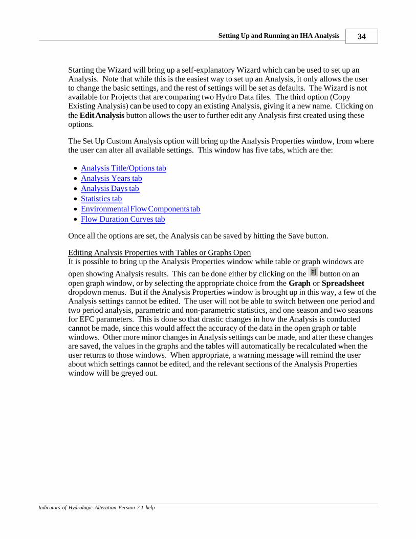
Setting Up and Running an IHA Analysis 34
Indicators of Hydrologic Alteration Version 7.1 help
Starting the Wizard will bring up a self-explanatory Wizard which can be used to set up anAnalysis. Note that while this is the easiest way to set up an Analysis, it only allows the userto change the basic settings, and the rest of settings will be set as defaults. The Wizard is notavailable for Projects that are comparing two Hydro Data files. The third option (CopyExisting Analysis) can be used to copy an existing Analysis, giving it a new name. Clicking onthe Edit Analysis button allows the user to further edit any Analysis first created using theseoptions.
The Set Up Custom Analysis option will bring up the Analysis Properties window, from wherethe user can alter all available settings. This window has five tabs, which are the:
· Analysis Title/Options tab· Analysis Years tab· Analysis Days tab· Statistics tab· Environmental Flow Components tab· Flow Duration Curves tab
Once all the options are set, the Analysis can be saved by hitting the Save button.
Editing Analysis Properties with Tables or Graphs OpenIt is possible to bring up the Analysis Properties window while table or graph windows are
open showing Analysis results. This can be done either by clicking on the button on anopen graph window, or by selecting the appropriate choice from the Graph or Spreadsheetdropdown menus. But if the Analysis Properties window is brought up in this way, a few of theAnalysis settings cannot be edited. The user will not be able to switch between one period andtwo period analysis, parametric and non-parametric statistics, and one season and two seasonsfor EFC parameters. This is done so that drastic changes in how the Analysis is conductedcannot be made, since this would affect the accuracy of the data in the open graph or tablewindows. Other more minor changes in Analysis settings can be made, and after these changesare saved, the values in the graphs and the tables will automatically be recalculated when theuser returns to those windows. When appropriate, a warning message will remind the userabout which settings cannot be edited, and the relevant sections of the Analysis Propertieswindow will be greyed out.
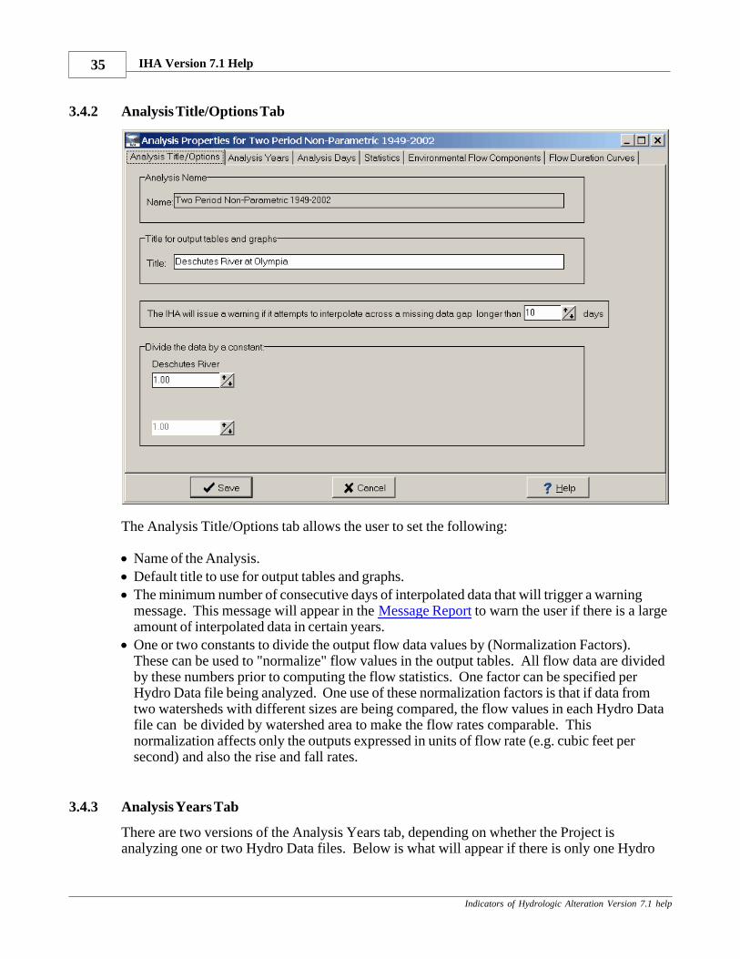
IHA Version 7.1 Help35
Indicators of Hydrologic Alteration Version 7.1 help
3.4.2 Analysis Title/Options Tab
The Analysis Title/Options tab allows the user to set the following:
· Name of the Analysis.· Default title to use for output tables and graphs.· The minimum number of consecutive days of interpolated data that will trigger a warning
message. This message will appear in the Message Report to warn the user if there is a largeamount of interpolated data in certain years.
· One or two constants to divide the output flow data values by (Normalization Factors). These can be used to "normalize" flow values in the output tables. All flow data are dividedby these numbers prior to computing the flow statistics. One factor can be specified perHydro Data file being analyzed. One use of these normalization factors is that if data fromtwo watersheds with different sizes are being compared, the flow values in each Hydro Datafile can be divided by watershed area to make the flow rates comparable. Thisnormalization affects only the outputs expressed in units of flow rate (e.g. cubic feet persecond) and also the rise and fall rates.
3.4.3 Analysis Years Tab
There are two versions of the Analysis Years tab, depending on whether the Project isanalyzing one or two Hydro Data files. Below is what will appear if there is only one Hydro
Setting Up and Running an IHA Analysis 36
Indicators of Hydrologic Alteration Version 7.1 help
Data file. This tab allows the user to choose between single period and two period analysis,and to set the water years to be used for analysis. It will display the range of years available inthe Hydro Data file, and the user can use slider bars to specify which years will be used foranalysis. The two Hydro Data file version is similar, with a slider bar for each of the HydroData files. Note that the begin and end water year settings cannot correspond to water yearsthat are missing from the Hydro Data file, and the Analysis cannot be saved until this problemis corrected.
If the Analysis Years tab is displayed while a table or graph from the current Analysis is open,it will not be possible to switch between one period and two period analysis (see EditingAnalysis Properties with Tables or Graphs Open).
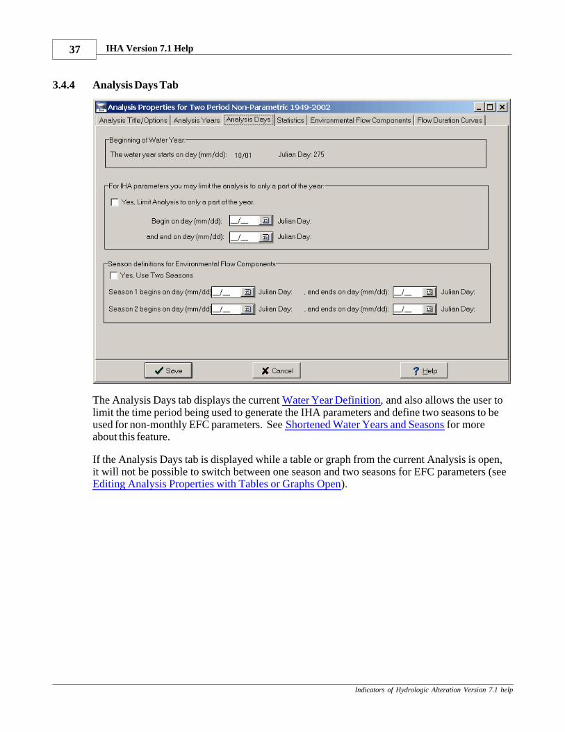
IHA Version 7.1 Help37
Indicators of Hydrologic Alteration Version 7.1 help
3.4.4 Analysis Days Tab
The Analysis Days tab displays the current Water Year Definition, and also allows the user tolimit the time period being used to generate the IHA parameters and define two seasons to beused for non-monthly EFC parameters. See Shortened Water Years and Seasons for moreabout this feature.
If the Analysis Days tab is displayed while a table or graph from the current Analysis is open,it will not be possible to switch between one season and two seasons for EFC parameters (see Editing Analysis Properties with Tables or Graphs Open).
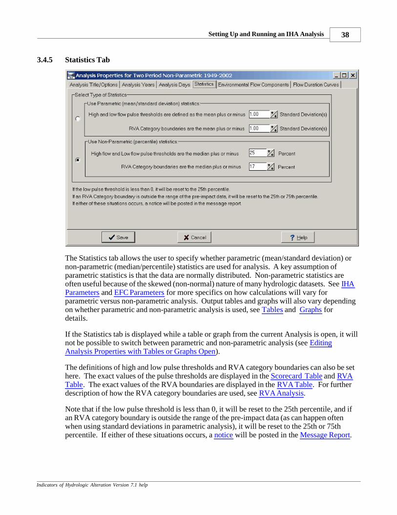
Setting Up and Running an IHA Analysis 38
Indicators of Hydrologic Alteration Version 7.1 help
3.4.5 Statistics Tab
The Statistics tab allows the user to specify whether parametric (mean/standard deviation) ornon-parametric (median/percentile) statistics are used for analysis. A key assumption ofparametric statistics is that the data are normally distributed. Non-parametric statistics areoften useful because of the skewed (non-normal) nature of many hydrologic datasets. See IHAParameters and EFC Parameters for more specifics on how calculations will vary forparametric versus non-parametric analysis. Output tables and graphs will also vary dependingon whether parametric and non-parametric analysis is used, see Tables and Graphs fordetails.
If the Statistics tab is displayed while a table or graph from the current Analysis is open, it willnot be possible to switch between parametric and non-parametric analysis (see EditingAnalysis Properties with Tables or Graphs Open).
The definitions of high and low pulse thresholds and RVA category boundaries can also be sethere. The exact values of the pulse thresholds are displayed in the Scorecard Table and RVATable. The exact values of the RVA boundaries are displayed in the RVA Table. For furtherdescription of how the RVA category boundaries are used, see RVA Analysis.
Note that if the low pulse threshold is less than 0, it will be reset to the 25th percentile, and ifan RVA category boundary is outside the range of the pre-impact data (as can happen oftenwhen using standard deviations in parametric analysis), it will be reset to the 25th or 75thpercentile. If either of these situations occurs, a notice will be posted in the Message Report.
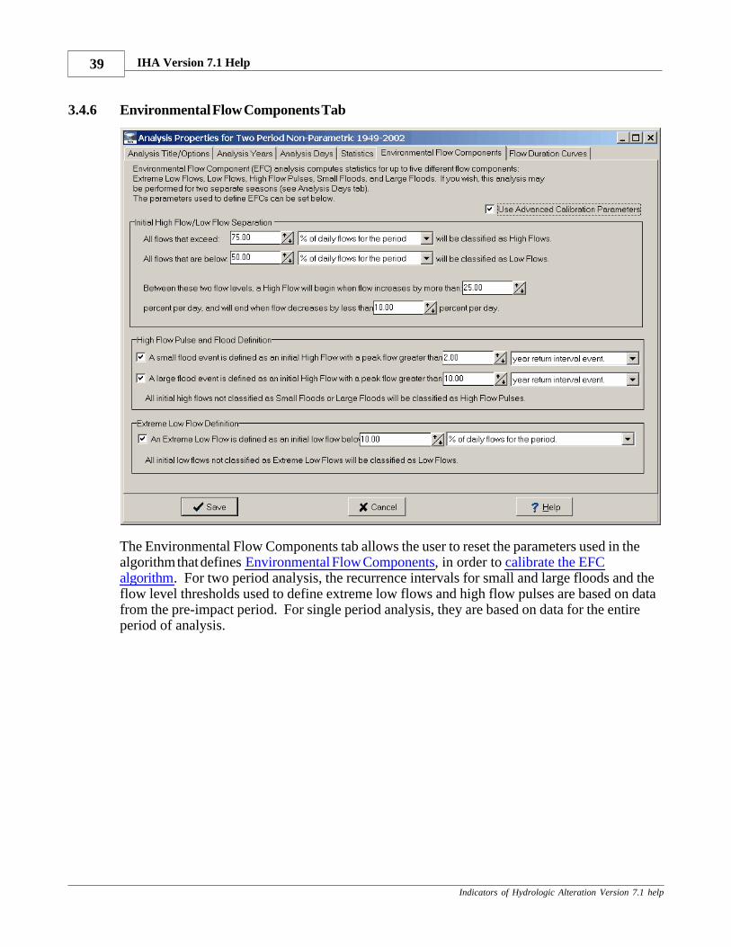
IHA Version 7.1 Help39
Indicators of Hydrologic Alteration Version 7.1 help
3.4.6 Environmental Flow Components Tab
The Environmental Flow Components tab allows the user to reset the parameters used in thealgorithm that defines Environmental Flow Components, in order to calibrate the EFCalgorithm. For two period analysis, the recurrence intervals for small and large floods and theflow level thresholds used to define extreme low flows and high flow pulses are based on datafrom the pre-impact period. For single period analysis, they are based on data for the entireperiod of analysis.
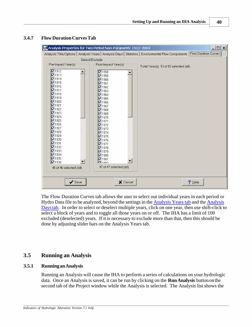
Setting Up and Running an IHA Analysis 40
Indicators of Hydrologic Alteration Version 7.1 help
3.4.7 Flow Duration Curves Tab
The Flow Duration Curves tab allows the user to select out individual years in each period orHydro Data file to be analyzed, beyond the settings in the Analysis Years tab and the AnalysisDays tab. In order to select or deselect multiple years, click on one year, then use shift-click toselect a block of years and to toggle all those years on or off. The IHA has a limit of 100excluded (deselected) years. If it is necessary to exclude more than that, then this should bedone by adjusting slider bars on the Analysis Years tab.
3.5 Running an Analysis
3.5.1 Running an Analysis
Running an Analysis will cause the IHA to perform a series of calculations on your hydrologicdata. Once an Analysis is saved, it can be run by clicking on the Run Analysis button on thesecond tab of the Project window while the Analysis is selected. The Analysis list shows the
IHA Version 7.1 Help41
Indicators of Hydrologic Alteration Version 7.1 help
last date and time that the Analysis was run. If the Run Analysis button has not been clickedon, selecting any of the options from the View Results button will also automatically run theAnalysis.
Note that if after running an Analysis, the user makes any changes to the Hydro Data file, theparameters on the Project Definition tab of the Project window, or any of the Analysis settingsor parameters, the Analysis will automatically be rerun whenever the user tries to view anyresults of the Analysis. This will occur if the user makes a selection from the View Resultsbutton, or clicks on a table or graph window that was left open while the Analysis settingswere being changed. This latter recalculation is done to ensure that there will never be anydata in an open table or graph that is not consistent with the current Analysis settings. Thisfeature also allows the user to quickly switch between the Analysis Properties window and thetables and graphs, which can be useful when Calibrating the EFC Algorithm or adjusting otherAnalysis settings based on the results.
3.5.2 Batch Analysis
IHA Analyses can also be run in a batch mode. The window described below will create anidentical Analysis for each of a number of Hydro Data files. These Analyses will differ only inthe years analyzed. Note that when a Batch Analysis is set up and run, it will create and run aseparate Analysis for each of the Hydro Data files in the current working directory, deletingany existing results. So it is best to create specialized working directories for conductingBatch Analyses. Batch analysis can only be conducted for one Hydro Data file analyses, notfor comparisons of two Hydro Data files.
Batch processing can be initiated by clicking IHA | Batch Processing. This will bring up thefollowing window:
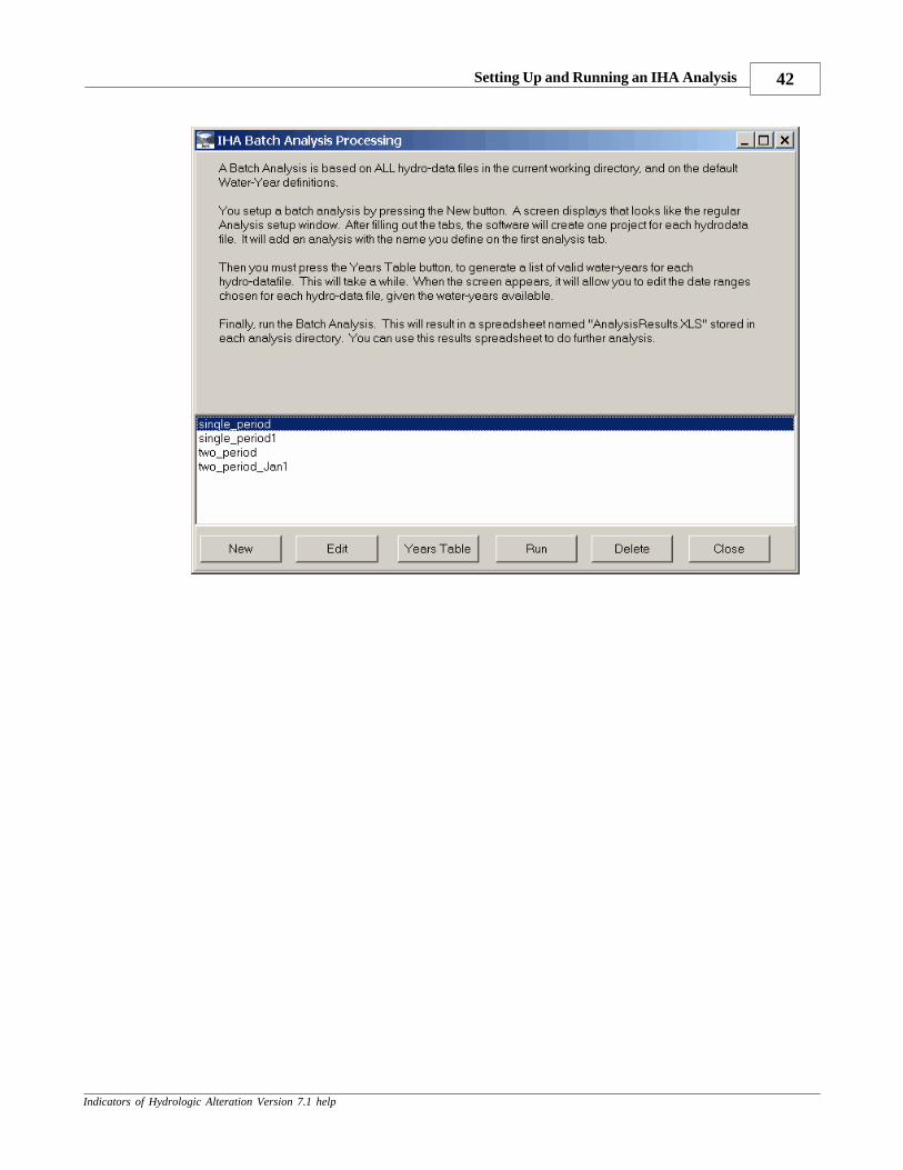
Setting Up and Running an IHA Analysis 42
Indicators of Hydrologic Alteration Version 7.1 help
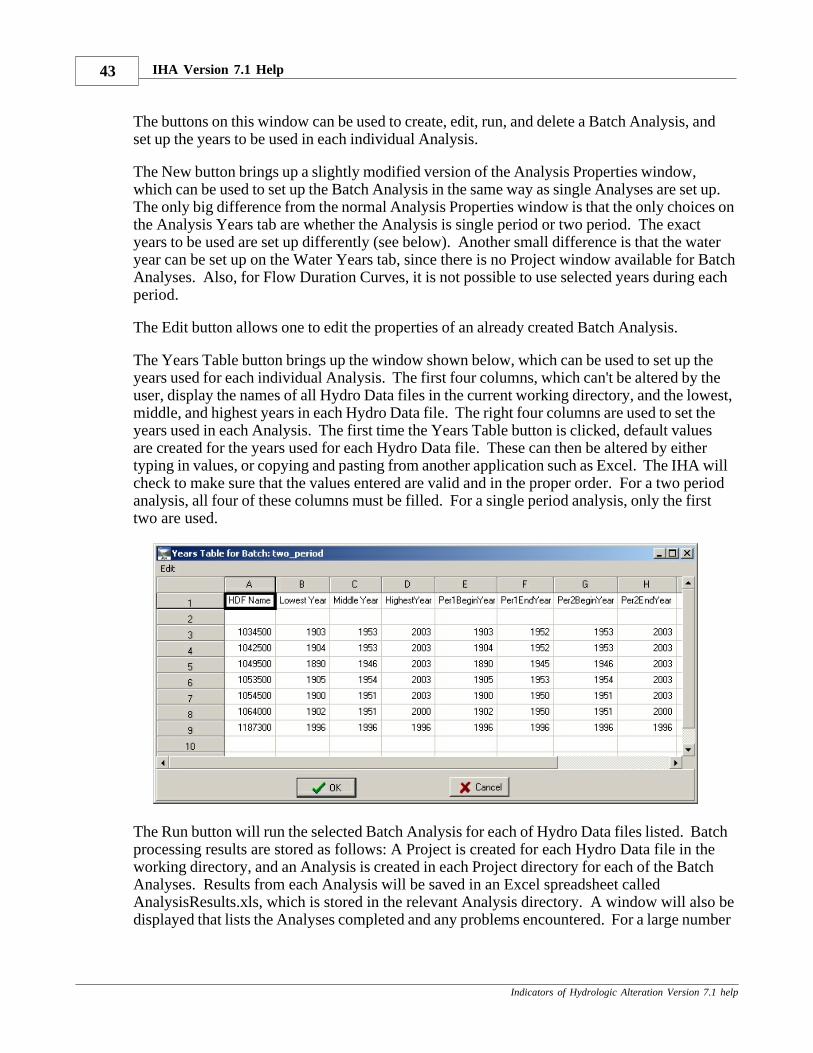
IHA Version 7.1 Help43
Indicators of Hydrologic Alteration Version 7.1 help
The buttons on this window can be used to create, edit, run, and delete a Batch Analysis, andset up the years to be used in each individual Analysis.
The New button brings up a slightly modified version of the Analysis Properties window,which can be used to set up the Batch Analysis in the same way as single Analyses are set up. The only big difference from the normal Analysis Properties window is that the only choices onthe Analysis Years tab are whether the Analysis is single period or two period. The exactyears to be used are set up differently (see below). Another small difference is that the wateryear can be set up on the Water Years tab, since there is no Project window available for BatchAnalyses. Also, for Flow Duration Curves, it is not possible to use selected years during eachperiod.
The Edit button allows one to edit the properties of an already created Batch Analysis.
The Years Table button brings up the window shown below, which can be used to set up theyears used for each individual Analysis. The first four columns, which can't be altered by theuser, display the names of all Hydro Data files in the current working directory, and the lowest,middle, and highest years in each Hydro Data file. The right four columns are used to set theyears used in each Analysis. The first time the Years Table button is clicked, default valuesare created for the years used for each Hydro Data file. These can then be altered by eithertyping in values, or copying and pasting from another application such as Excel. The IHA willcheck to make sure that the values entered are valid and in the proper order. For a two periodanalysis, all four of these columns must be filled. For a single period analysis, only the firsttwo are used.
The Run button will run the selected Batch Analysis for each of Hydro Data files listed. Batchprocessing results are stored as follows: A Project is created for each Hydro Data file in theworking directory, and an Analysis is created in each Project directory for each of the BatchAnalyses. Results from each Analysis will be saved in an Excel spreadsheet calledAnalysisResults.xls, which is stored in the relevant Analysis directory. A window will also bedisplayed that lists the Analyses completed and any problems encountered. For a large number

Setting Up and Running an IHA Analysis 44
Indicators of Hydrologic Alteration Version 7.1 help
of Hydro Data files, be aware that batch processing can be time-consuming. Results ofProjects created through batch processing can also be viewed individually in the same way asnormal results are viewed.
3.6 Other Features
3.6.1 Graph Default Settings
In order to reduce the need to edit each individual graph, many of which have very similarfeatures, the IHA allows the user to edit the characteristics of a default set of graphs, whosesettings are then used to populate all subsequent graphs that are created in any Project. Thesedefault graphs can be accessed by clicking on Options | Graph Default Layout. There areseparate default graphs for the single period annual data graphs, two period annual data graphs(with separate defaults for graphs with RVA lines and variance lines), monthly average graph,hydrologic alteration graph, flow duration curves, and daily data graphs (with separate defaultsfor daily data with and without Environmental Flow Components). An example default graphis shown below.
These default graphs can be edited just like the normal graphs (see Editing and Working withIHA Graphs), and once they are saved any new graphs of the same type created in any Analysiswill use all the same features (fonts, colors, line symbols, etc.) of the default graphs. If you
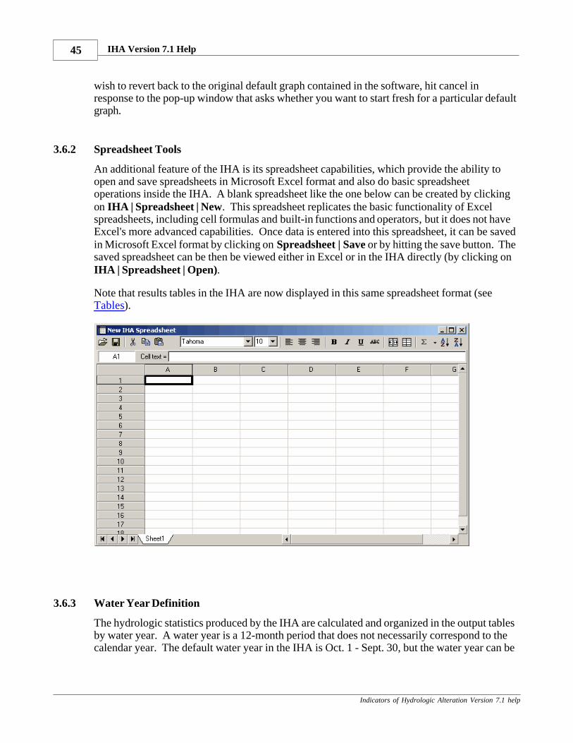
IHA Version 7.1 Help45
Indicators of Hydrologic Alteration Version 7.1 help
wish to revert back to the original default graph contained in the software, hit cancel inresponse to the pop-up window that asks whether you want to start fresh for a particular defaultgraph.
3.6.2 Spreadsheet Tools
An additional feature of the IHA is its spreadsheet capabilities, which provide the ability toopen and save spreadsheets in Microsoft Excel format and also do basic spreadsheetoperations inside the IHA. A blank spreadsheet like the one below can be created by clickingon IHA | Spreadsheet | New. This spreadsheet replicates the basic functionality of Excelspreadsheets, including cell formulas and built-in functions and operators, but it does not haveExcel's more advanced capabilities. Once data is entered into this spreadsheet, it can be savedin Microsoft Excel format by clicking on Spreadsheet | Save or by hitting the save button. Thesaved spreadsheet can be then be viewed either in Excel or in the IHA directly (by clicking on IHA | Spreadsheet | Open).
Note that results tables in the IHA are now displayed in this same spreadsheet format (see Tables).
3.6.3 Water Year Definition
The hydrologic statistics produced by the IHA are calculated and organized in the output tablesby water year. A water year is a 12-month period that does not necessarily correspond to thecalendar year. The default water year in the IHA is Oct. 1 - Sept. 30, but the water year can be
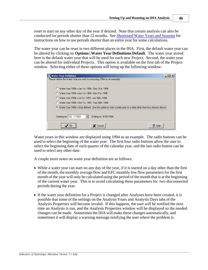
Setting Up and Running an IHA Analysis 46
Indicators of Hydrologic Alteration Version 7.1 help
reset to start on any other day of the year if desired. Note that certain analysis can also beconducted for periods shorter than 12 months. See Shortened Water Years and Seasons forinstructions on how to use periods shorter than an entire year for some calculations.
The water year can be reset in two different places in the IHA. First, the default water year canbe altered by clicking on Options | Water Year Definitions Default. The water year storedhere is the default water year that will be used for each new Project. Second, the water yearcan be altered for individual Projects. This option is available on the first tab of the Projectwindow. Selecting either of these options will bring up the following window:
Water years in this window are displayed using 1994 as an example. The radio buttons can beused to select the beginning of the water year. The first four radio buttons allow the user toselect the beginning date of each quarter of the calendar year, and the last radio button can beused to select any other date.
A couple more notes on water year definition are as follows:
· While a water year can start on any day of the year, if it is started on a day other than the firstof the month, the monthly average flow and EFC monthly low flow parameters for the firstmonth of the year will only be calculated using the period of the month that is at the beginningof the current water year. This is to avoid calculating these parameters for two disconnectedperiods during the year.
· If the water year definition for a Project is changed after Analyses have been created, it ispossible that some of the settings on the Analysis Years and Analysis Days tabs of theAnalysis Properties will become invalid. If this happens, the user will be notified the nexttime an Analysis is run, and the Analysis Properties window will be displayed so the neededchanges can be made. Sometimes the IHA will make these changes automatically, andsometimes it will display a warning message notifying the user where the problem is.
IHA Version 7.1 Help47
Indicators of Hydrologic Alteration Version 7.1 help
3.6.4 Working Directory
The IHA software stores all of the data and information associated with saved Hydro Datafiles, Projects, and output tables and graphs in a single directory, called the working directory.The default working directory is the same directory that the IHA is installed in, and undernormal use there should be no need to ever change this directory. But if the user does wish tocontrol where the IHA stores its data, the working directory can be reset by clicking on Options | Set Working Directory, and selecting another directory. Note that the only HydroData files and Projects that will be accessible to the user are those that are saved in the currentworking directory. The current working directory is also displayed in Project Definition tab ofthe Project window.
The working directory contains two subdirectories named HydroData and Projects, whichcontain all the data and other information that is currently saved. If it is necessary to transferIHA data from one computer, hard-drive, or directory to another, this can be done by copyingthese two subdirectories directly. Each Project directory also contains subdirectories for eachindividual Project and for each Analysis with each Project.
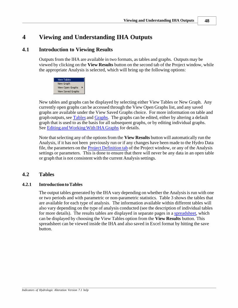
Viewing and Understanding IHA Outputs 48
Indicators of Hydrologic Alteration Version 7.1 help
4 Viewing and Understanding IHA Outputs
4.1 Introduction to Viewing Results
Outputs from the IHA are available in two formats, as tables and graphs. Outputs may beviewed by clicking on the View Results button on the second tab of the Project window, whilethe appropriate Analysis is selected, which will bring up the following options:
New tables and graphs can be displayed by selecting either View Tables or New Graph. Anycurrently open graphs can be accessed through the View Open Graphs list, and any savedgraphs are available under the View Saved Graphs choice. For more information on table andgraph outputs, see Tables and Graphs. The graphs can be edited, either by altering a defaultgraph that is used to as the basis for all subsequent graphs, or by editing individual graphs. See Editing and Working With IHA Graphs for details.
Note that selecting any of the options from the View Results button will automatically run theAnalysis, if it has not been previously run or if any changes have been made to the Hydro Datafile, the parameters on the Project Definition tab of the Project window, or any of the Analysissettings or parameters. This is done to ensure that there will never be any data in an open tableor graph that is not consistent with the current Analysis settings.
4.2 Tables
4.2.1 Introduction to Tables
The output tables generated by the IHA vary depending on whether the Analysis is run with oneor two periods and with parametric or non-parametric statistics. Table 3 shows the tables thatare available for each type of analysis. The information available within different tables willalso vary depending on the type of analysis conducted (see the description of individual tablesfor more details). The results tables are displayed in separate pages in a spreadsheet, whichcan be displayed by choosing the View Tables option from the View Results button. Thisspreadsheet can be viewed inside the IHA and also saved in Excel format by hitting the savebutton.
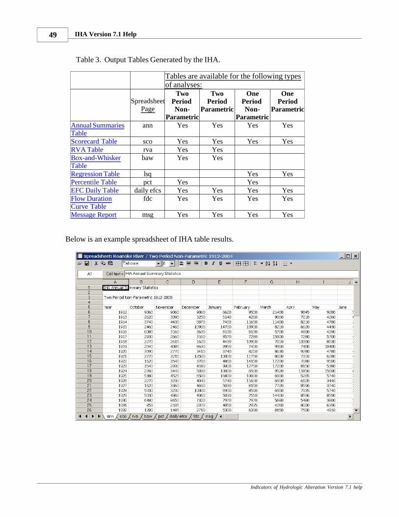
IHA Version 7.1 Help49
Indicators of Hydrologic Alteration Version 7.1 help
Table 3. Output Tables Generated by the IHA.
Tables are available for the following typesof analyses:
SpreadsheetPage
TwoPeriod Non-
Parametric
TwoPeriod
Parametric
OnePeriod Non-
Parametric
OnePeriod
Parametric
Annual SummariesTable
ann Yes Yes Yes Yes
Scorecard Table sco Yes Yes Yes YesRVA Table rva Yes YesBox-and-WhiskerTable
baw Yes Yes
Regression Table lsq Yes YesPercentile Table pct Yes YesEFC Daily Table daily efcs Yes Yes Yes YesFlow DurationCurve Table
fdc Yes Yes Yes Yes
Message Report msg Yes Yes Yes Yes
Below is an example spreadsheet of IHA table results.
Viewing and Understanding IHA Outputs 50
Indicators of Hydrologic Alteration Version 7.1 help
The first time a results spreadsheet is viewed, the Message Report is displayed on top, so thatthe user can see any messages and warnings from the Analysis.
When a spreadsheet containing output tables from an Analysis is displayed, the options on the Spreadsheet dropdown menu can be used to display the current Analysis Properties window,the current Project window, the Hydro Data file that was used for the Analysis, and any graphsthat are related to this Analysis.
Note that if the Analysis Properties window is brought up while a spreadsheet is beingdisplayed, certain settings of the Analysis cannot be altered (see Editing Analysis Propertieswith Tables or Graphs Open). If any changes are made to the Analysis Properties, the values inthe spreadsheet will automatically be recalculated when the user returns to that window. Thisis done to ensure that there will never be any data in an open table that is not consistent with thecurrent Analysis settings.
Below are a couple more notes about IHA results tables:
· IHA results are displayed with four significant digits.
· Usually, at least a few of the cells in some of these tables will be blank. This occurs whenno valid data existed to calculate the parameter or statistic held in that cell.
· If two seasons are used when calculating EFCs, the number of rows and columns in eachtable will be increased in order to display individual parameter values for two seasonsinstead of one.
4.2.2 Annual Summaries Table
This table displays all the IHA and EFC parameter values for each individual water year thathas been included in the time periods selected for analysis. Each column shows one parameter,and each row corresponds to one year. Note that if your input flow data has any water yearswhich have no valid flow values, these years will not have rows in this table.
If non-parametric statistics were used, the values in this table are medians for each water yearof the relevant sub-annual data. So for example: for October flows, the value in this table is themedian of all daily flows during October in the water year; for high pulse durations, the valuein this table is the median of the durations of all high pulse events in the water year; etc.
If parametric statistics are used, the values in this table are means rather than medians.
For comparisons of two Hydro Data files, all the water years for the file that is selected as pre-impact will be shown first (at the top), followed by all the years for the file used as post-impact.
IHA Version 7.1 Help51
Indicators of Hydrologic Alteration Version 7.1 help
4.2.3 Scorecard Table
This table shows a variety of statistics for the pre-impact and post-impact periods (or for thetwo Hydro Data files being compared), for each hydrologic parameter. These statistics arecalculated from the annual values in the Annual Summaries Table. The statistics will varydepending on whether the analysis was run with parametric or non-parametric statistics. Forsingle period analysis, fewer columns will be shown in the table, since there is not pre-impactand post-impact periods.
The Scorecard Table also shows the high and low pulse thresholds (under the section forParameter Group #4), and the flow values that correspond to the five EFC calibrationparameters (below all of the EFC data).
Non-Parametric Scorecard Table
The header panel contains a number of parameters that apply only to the period of analysis as awhole. These are:
· Normalization Factor. This is the normalization factor entered in Analysis Title/OptionsTab. All output flow values have been divided by this factor (except the Non-NormalizedMean Flow below). If two Hydro Data files are being used, each can have a differentnormalization factor, and both will be displayed here.
· Mean annual flow · Non-Normalized Mean Flow· Annual Coefficient of Variation. This is calculated as the standard deviation of all the daily
flow values, divided by the mean annual flow.· Flow predictability. Predictability ranges in value from 0 to 1 and is composed of two
additive components: constancy (C), a measure of temporal invariance, and contingency(M), a measure of periodicity. The predictability of a stream with very constant flow willbe mostly due to C, while the predictability of a stream with highly variable flow with afixed periodicity will be mostly due to M.
· Flow constancy / flow predictability. C / (C+M). · Maximum proportion of floods that occur during any common 60 day period in all years
during the period of record. Floods are defined as any flows above the high pulse threshold.See the Statistics tab of the Analysis Properties window to set this threshold.
· Length of flood-free season. This is the length in days of the longest period common to allwater years where flows are at or below the high pulse threshold in every year.
These parameters are modeled after a suite of parameters described by Poff and Ward (1989). The flow predictability, constancy, and contingency measures are originally from Colwell(1974). If a shortened water year is used for IHA parameters, the parameters in the headerpanel will be calculated only for that shortened period.
The rest of the data in the table consists of a series of columns which display statistics for eachhydrologic parameter. The columns displayed for two period analysis are as follows:
Columns 1 and 2 display the median (i.e. the 50th percentile) for each of the two periods.
Viewing and Understanding IHA Outputs 52
Indicators of Hydrologic Alteration Version 7.1 help
Columns 3 and 4 display the coefficients of dispersion (CD) for each period. This isdefined as = (75th percentile - 25th percentile) / 50th percentile.
Columns 5 and 6 show the deviation of the post-impact period from the pre-impact. This isdefined as Deviation Factor = |(Post-impact value) - (Pre-impact value)| / (Pre-impactvalue). This deviation is shown both for the median and for the coefficient of dispersion.
Columns 7 and 8 calculate a "significance count" for the deviation values. To calculatethis, the software program randomly shuffles all years of input data and recalculates(fictitious) pre- and post-impact medians and CDs 1000 times. The significance count isthe fraction of trials for which the deviation values for the medians or CDs were greaterthan for the real case. So a low significance count (minimum value is 0) means that thedifference between the pre- and post-impact periods is highly significant, and a highsignificance count (maximum value is 1) means that there is little difference between thepre- and post-impact periods. The significance count can be interpreted similarly to a p-value in parametric statistics.
It is important to understand that in some infrequent situations this algorithm maygenerate very low significance counts when there is very little apparent differencebetween the pre- and post-impact periods. This can occur when the deviation factorbetween the pre- and post-impact periods is zero or very small, and the overalldistribution contains a large number of values right at or very near the center of thedistribution. In this situation a low significance count actually means that the lack ofdifference between the two periods is highly significant, in a statistical sense, becauserandomly rearranging the data rarely yield a larger deviation factor than the originaldata.
It is also important to understand that significance counts may differ slightly each timethe IHA is run for the same dataset, since a new set of randomized cases is generatedeach time.
For single period analysis, only columns 1 and 3 are displayed, showing data for the singleperiod.
Parametric Scorecard Table
The header panel is identical for the parametric version of this table.
The columns in the main body of the table are slightly different, and are organized as follows:
Columns 1 and 2 are the means for each period
Columns 3 and 4 are the coefficients of variation, defined as (standard deviation) / mean.
Column 5 gives the magnitude of the change in mean values from the pre-impact to the post-impact period, called the deviation factor.
IHA Version 7.1 Help53
Indicators of Hydrologic Alteration Version 7.1 help
Column 6 expresses this change as a percentage.
Columns 7 and 8 give the magnitude and percentage change in the coefficients of variation.
For each IHA parameter group, the absolute values of the percentage change in the deviationfactors of the mean and coefficient of variation are averaged. These means are shown at thebottoms of the respective column, and offer an at-a-glance summary of the impact on eachparameter group.
As with the non-parametric version of the table, for single period analysis, only columns 1 and3 are displayed, showing data for the single period.
4.2.4 RVA Table
This table shows the results that are used for RVA Analysis, which is done for IHA parametersonly. Results are shown either for the pre-impact and post-impact periods, or for the twoHydro Data files being compared. These statistics are calculated from the annual values in the Annual Summaries Table. The RVA Table also shows the high and low pulse thresholds(under the section for Parameter Group #4)
The first section of this table gives the following information on each of the hydrologicparameters:
Columns 1-2 show the median or mean and coefficient of dispersion ((75th percentile - 25thpercentile) / 50th percentile) or coefficient of variation ((standard deviation) / mean), forthe pre-impact period. What is shown in these columns depends on whether parametric ornon-parametric statistics are used.
Columns 3-4 show the minimum and maximum for each parameter during the pre-impactperiod.
Columns 5-8 give the same information as Columns 1-4 for the post-impact period.
Columns 9-10 give the low and high RVA category boundaries. These values arecalculated according to the settings in the Statistics tab of the Set Up Analysis window.
Column 11 gives the Hydrologic Alteration factor for the middle RVA category.
The second section of the table compares the distributions of data in each of the three RVAcategories. Expected and observed frequencies and the Hydrologic Alteration factor are shownseparately for each of the three RVA categories.
See RVA Analysis for a description of how expected and observed frequencies and HydrologicAlteration factors are calculated.

Viewing and Understanding IHA Outputs 54
Indicators of Hydrologic Alteration Version 7.1 help
4.2.5 Box-and-Whisker Table
This table contains five values for each hydrologic parameter, for the pre-impact and post-impact periods (or for the two Hydro Data files being compared). These statistics arecalculated from the annual values in the Annual Summaries Table. For non-parametricanalysis, it shows the median, 25th and 75th percentile values, and minimum and maximumvalues. For parametric analysis, it shows the mean, the mean plus and minus 1 standarddeviation, and minimum and maximum values. Note that for the parametric analysis, the meanplus or minus 1 standard deviation may end up being greater than the minimum or maximumvalue or event negative, depending on how the data is distributed.
These values are for use in creating box-and-whisker plots.
4.2.6 Regression Table
This table shows complete results from a linear regression on each hydrologic parameterduring the period of record (for single period analysis only). These statistics are calculatedfrom the annual values in the Annual Summaries Table. The table shows the following for eachparameter:
Columns 1 and 2 show the slope and y-intercept of the least-squares fit regression line.
Column 3 shows sigma (standard error of the predicted y-value for each x in theregression). This is the standard deviation of the residuals of the regression.
Column 4 shows the correlation coefficient.
Column 5 shows the P-value for the slope of the regression line.
Column 6 shows the F statistic for the regression line.
Column 7 shows the R2 for the regression line.
4.2.7 Percentile Table
This table shows the details of the percentile statistics. Results are shown either for the pre-impact and post-impact periods, or for the two Hydro Data files being compared. Thesestatistics are calculated from the annual values in the Annual Summaries Table. For two periodanalysis, there are 12 columns. The first five columns show the 10th, 25th, 50th, 75th, and 90thpercentile values for the pre-impact period. The sixth column has the coefficient of dispersion,calculated as (75th percentile - 25th percentile) / 50th percentile. The last six columns give theanalogous values for the post-impact period. For single period analysis, only six columns areshown, showing the analogous values for the entire period.
IHA Version 7.1 Help55
Indicators of Hydrologic Alteration Version 7.1 help
4.2.8 EFC Daily Table
This table shows the Environmental Flow Component (EFC) event types that are assigned toeach day of flow. It has five columns, which show the calendar date, the volume of flow, acode for the EFC type (0 = extreme low flow, 1 = low flow, 2 = high flow pulse, 3 = smallflood, 4 = large flood), the EFC type, and whether or not the row contains real or interpolatedflow data. Note that if your input flow data has any water years which have no valid flowvalues, these years will not have rows in this table.
4.2.9 Flow Duration Curve Table
This table shows results for Flow Duration Curves (FDCs). For each period being analyzed orHydro Data file being compared, there are 26 columns, showing the flow values (ranked fromhighest to lowest) and exceedance probability, for all the data (the annual FDC) and for eachmonth (monthly FDCs). So for one period analysis, there are 26 columns, and for a two periodanalysis and a comparison of two Hydro Data files, there are 52 columns.
The specific years and days of data used for the annual FDCs are according to the settings onthe Analysis Years tab, the Analysis Days tab, and the Flow Duration Curves tab. To simplifycomputations, the data used for the monthly FDCs are according to the settings on the AnalysisYears tab and Flow Duration Curves tab only. So specifying a shortened water year on theAnalysis Days tab will only affect the annual FDC, not the monthly FDCs.
4.2.10 Message Report
This report shows any message and warnings generated while running your Analysis. Pleaseread this report carefully, because there may be important warnings about possible problemswith your results. See Warning Messages for a description of all the possible warnings.
4.3 Graphs
4.3.1 Introduction to Graphs
Choosing the View Graphs option from the View Results will bring up the IHA Graph Optionswindow below, which can be used to select the type of graph to be displayed and also altersome of the basic features on the graph. Some of the options displayed on these windows willvary depending on whether your analysis is one period or two period and parametric or non-parametric. Choosing the View Saved Graphs option from the View Results button will bringup a list of saved graphs. For more on graphs, see Summary of IHA Graphs and Editing andWorking with IHA Graphs.
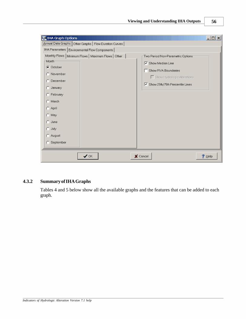
Viewing and Understanding IHA Outputs 56
Indicators of Hydrologic Alteration Version 7.1 help
4.3.2 Summary of IHA Graphs
Tables 4 and 5 below show all the available graphs and the features that can be added to eachgraph.
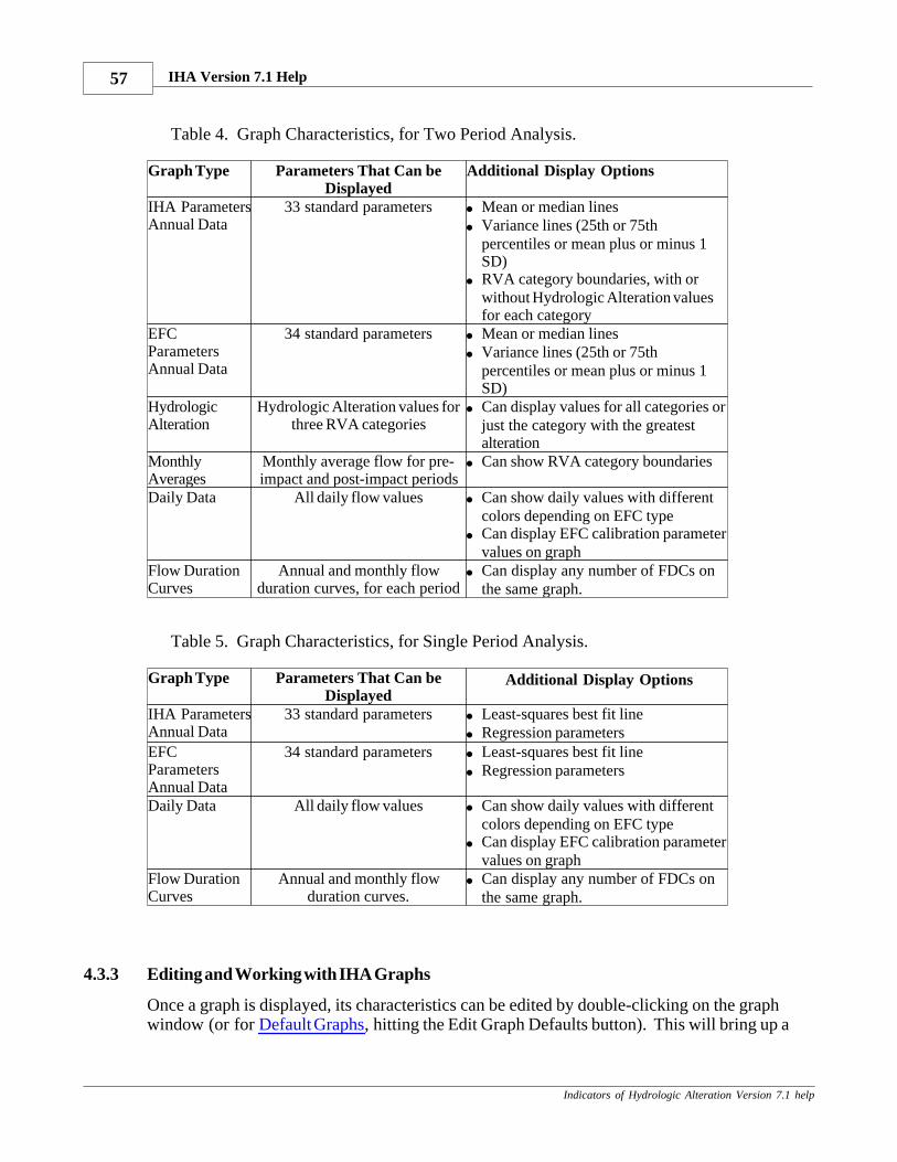
IHA Version 7.1 Help57
Indicators of Hydrologic Alteration Version 7.1 help
Table 4. Graph Characteristics, for Two Period Analysis.
Graph Type Parameters That Can beDisplayed
Additional Display Options
IHA ParametersAnnual Data
33 standard parameters · Mean or median lines
· Variance lines (25th or 75thpercentiles or mean plus or minus 1SD)
· RVA category boundaries, with orwithout Hydrologic Alteration valuesfor each category
EFCParametersAnnual Data
34 standard parameters · Mean or median lines
· Variance lines (25th or 75thpercentiles or mean plus or minus 1SD)
HydrologicAlteration
Hydrologic Alteration values forthree RVA categories
· Can display values for all categories orjust the category with the greatestalteration
MonthlyAverages
Monthly average flow for pre-impact and post-impact periods
· Can show RVA category boundaries
Daily Data All daily flow values · Can show daily values with differentcolors depending on EFC type
· Can display EFC calibration parametervalues on graph
Flow DurationCurves
Annual and monthly flowduration curves, for each period
· Can display any number of FDCs onthe same graph.
Table 5. Graph Characteristics, for Single Period Analysis.
Graph Type Parameters That Can beDisplayed
Additional Display Options
IHA ParametersAnnual Data
33 standard parameters · Least-squares best fit line
· Regression parametersEFCParametersAnnual Data
34 standard parameters · Least-squares best fit line
· Regression parameters
Daily Data All daily flow values · Can show daily values with differentcolors depending on EFC type
· Can display EFC calibration parametervalues on graph
Flow DurationCurves
Annual and monthly flowduration curves.
· Can display any number of FDCs onthe same graph.
4.3.3 Editing and Working with IHA Graphs
Once a graph is displayed, its characteristics can be edited by double-clicking on the graphwindow (or for Default Graphs, hitting the Edit Graph Defaults button). This will bring up a
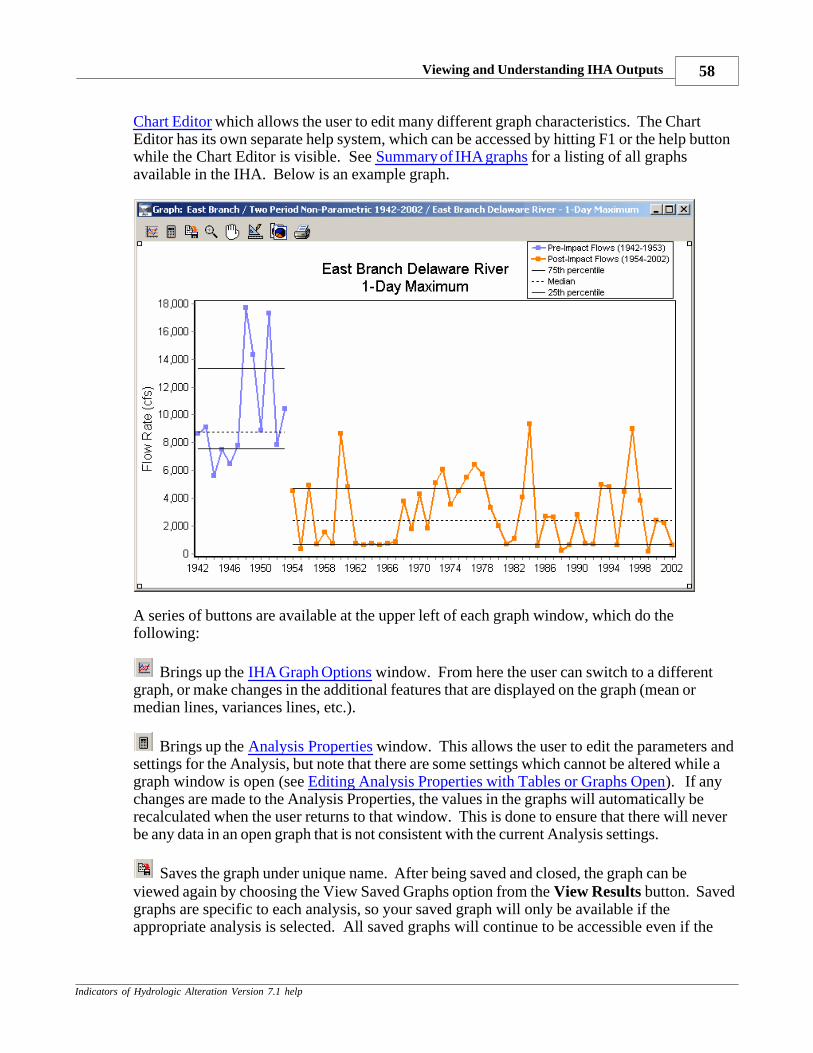
Viewing and Understanding IHA Outputs 58
Indicators of Hydrologic Alteration Version 7.1 help
Chart Editor which allows the user to edit many different graph characteristics. The ChartEditor has its own separate help system, which can be accessed by hitting F1 or the help buttonwhile the Chart Editor is visible. See Summary of IHA graphs for a listing of all graphsavailable in the IHA. Below is an example graph.
A series of buttons are available at the upper left of each graph window, which do thefollowing:
Brings up the IHA Graph Options window. From here the user can switch to a differentgraph, or make changes in the additional features that are displayed on the graph (mean ormedian lines, variances lines, etc.).
Brings up the Analysis Properties window. This allows the user to edit the parameters andsettings for the Analysis, but note that there are some settings which cannot be altered while agraph window is open (see Editing Analysis Properties with Tables or Graphs Open). If anychanges are made to the Analysis Properties, the values in the graphs will automatically berecalculated when the user returns to that window. This is done to ensure that there will neverbe any data in an open graph that is not consistent with the current Analysis settings.
Saves the graph under unique name. After being saved and closed, the graph can beviewed again by choosing the View Saved Graphs option from the View Results button. Savedgraphs are specific to each analysis, so your saved graph will only be available if theappropriate analysis is selected. All saved graphs will continue to be accessible even if the
IHA Version 7.1 Help59
Indicators of Hydrologic Alteration Version 7.1 help
Analysis settings have been altered and the Analysis re-run. Note that this is the only way tosaved edited features on a graph, if the graph is closed without saving, all changes will be lost.
Enables zoom capability. This feature is particularly useful when viewing the daily datagraphs. After enabling zoom capability by clicking on this button, click and hold the mousebutton and then draw a box over any area of the graph to zoom into that section of the graph. Tozoom back out to the full extent of the graph, click directly on the zoom button again.
Enables scroll capability. This feature is particularly useful when viewing the daily datagraphs. To scroll in any direction (after the enable scroll button has been selected), click andhold the mouse button and then move the hand in the desired direction.
Brings up the Chart Editor, which allows you to edit many different features of the graph.One particularly useful feature of the Chart Editor is the ability to re-draw the y-axis using alog scale. This can be done by clicking on the Chart tab in the Chart Editor, then the Axis tabbelow that, and then clicking the checkbox labeled Logarithmic (for the left axis). Note that ifthere are negative values on the y-axis, this option will not work, because it is impossible tocalculate logarithms for negative values. Also, after the y-axis has been reset to a log scale,this scale will be retained even if the graph window is switched to a different graph through theIHA Graph Options window.
Copies the graph onto your computer's clipboard.
Prints the graph.
Many of these options are also available on the Graph dropdown menu. It is also possiblefrom this menu to display the current Analysis Properties window, the current Project window,the Hydro Data file that was used for the Analysis, and the tables and any graphs that arerelated to this Analysis.
4.3.4 Chart Editor
The Chart Editor can be used to edit many different features of a graph, including the graphtitle, axis labels and title, colors and line types, text sizes and fonts, legend characteristics, andmuch more. The main Chart Editor window is displayed below. The Chart Editor has its ownseparate help system, which can be accessed by hitting F1 or the help button while the ChartEditor is visible.
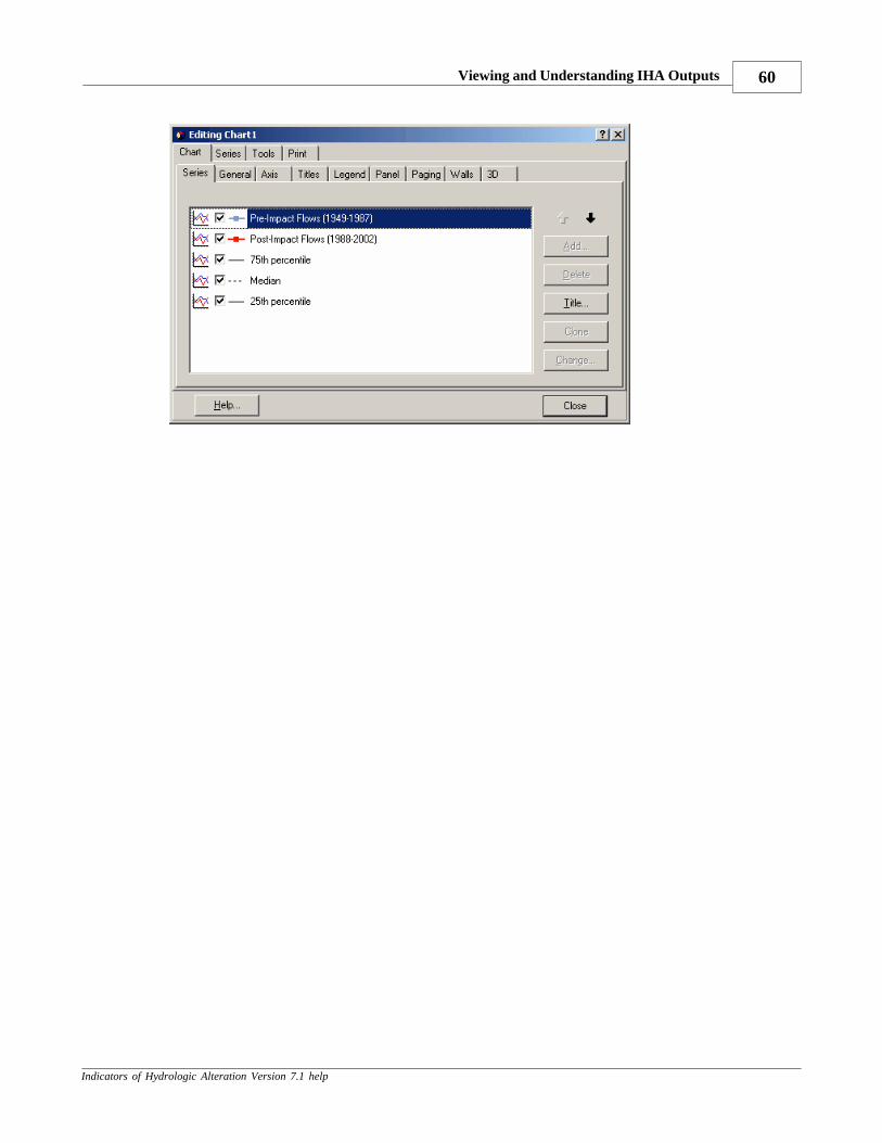
Viewing and Understanding IHA Outputs 60
Indicators of Hydrologic Alteration Version 7.1 help
IHA Version 7.1 Help61
Indicators of Hydrologic Alteration Version 7.1 help
5 Technical Notes
5.1 Introduction to Technical Notes
This section has some information that may be of interest to some IHA users. The followingissues are covered here:
· Calculation of empirical percentiles· Julian dates and methods for calculating statistics for timing variables· Handling of missing data values and data interpolation · Ability to conduct analysis for shortened water years or two separate seasons· Maximum number of years in Hydro Data files· Using the .par file as metadata for an IHA Analysis· Issues with large flow values· Warning messages· Bug-tracking feature· Regional and language settings· DOS Command line start-up
5.2 Empirical Percentiles
There is a problematic aspect to calculating non-parametric (percentile) statistics. Thereappears to be no general agreement on how to compute empirical percentiles for a finite dataset. We have chosen to use the algorithm in the International Mathematical and StatisticalLibraries (IMSL). You should be aware that some common statistical packages (notably thosein the Excel spreadsheet) use a different algorithm, and so will often produce different resultsfor the same set of data.
5.3 Julian Dates and Statistics for Timing Variables
In order to quantify the timings of maximum and minimum flows and EFC events, the IHA usesthe concept of Julian dates. Julian dates represent calendar dates by integer values, which startwith 1 on January 1 and end with 366 on December 31. Note that although the number ofcalendar days varies slightly in each year, depending on whether or not it is a leap year, thestarting and ending Julian dates in each year are always 1 and 366. In the IHA the differencebetween leap years and non-leap years is that leap years have a Julian date for Feb. 29, whichis 60, while non-leap years skip from Julian date 59 (Feb. 28) to Julian date 61 (Mar. 1). Thisensures that each calendar date is represented by the same Julian date in each year.
Users should be aware that this method of defining Julian dates does differ from definitionsused elsewhere, which usually assign a Julian date of 1 to January 1, 4713 B.C., and thenincrement the date by 1 for each day thereafter, without restarting the count at the beginning ofeach year.
Technical Notes 62
Indicators of Hydrologic Alteration Version 7.1 help
Leap years are all years that are divisible by 4 (i.e. 1996, 2000 etc.), except centurial years thatare not evenly divisible by 400 (i.e. 1700, 1800, 1900, 2100).
Calculating Statistics for Timing Variables Calculating means, medians, and other statistics for the IHA's timing parameters (the dates ofminimum and maximum flows and EFC events) presents some methodological problems,because of the difficulties of calculating statistics for any periodic variable (a date or time ofday, an angle). For instance, the arithmetic average of December 31 and January 2 (JulianDays 366 and 2) is day 184, which falls in July! The intuitive meaning of "average", however,requires a result of January 1. The methods for calculating statistics for the IHA's timingparameters are described below. The user should be warned that while these calculationmethods work reasonably well, in some cases the results generated by these methods are notideal. Because in some cases the calculation of statistics for timing related variables mayproduce peculiar and non-intuitive results, users should carefully review all the statistics fortiming parameters before using them in any analysis. These algorithms are unchanged fromearlier versions of the software, but improvement of these calculations is planned for futureversions of the software.
In order to deal with the difficulties of calculating statistics for timing variables, the IHA oftenuses a "circular method" for timing statistics. This method puts all the dates in question intoquarterly bins, which are 1-91, 92-183, 184-275, and 276-366 (depending on the situation,these bins are applied to either Julian dates or dates of the water year). If the second or thirdquarter has the greatest frequency of dates, the statistic is computed in the usual way. If thelargest number of dates is in the first quarter, 366 is temporarily subtracted from all dates in thefourth quarter prior to computing the statistic, and if the result is less than 0 then 366 is addedback onto it. If the largest number of dates is in the fourth quarter, 366 is temporarily added toall dates in the first quarter prior to computing the statistics, and if the result is greater than 366then 366 is subtracted from it. This method produces reasonable results in situations where thetiming values are clustered at some point in the year, although for variables where there is aneven distribution throughout the year, calculation of such statistics is unavoidably arbitrary.
There are a couple of warnings which can be generated in the Message Report because ofcalculation of these statistics. If more than 10% of the data falls in the quarter six months awayfrom the dominant quarter, a warning is generated. Here data are widely scattered throughoutthe year, meaning that statistics calculated using the "circular method" may not be toomeaningful. A second warning is also generated for parametric analysis if the standarddeviation calculated using the "circular method" is greater than 180, indicating a similarsituation.
All of the statistics calculated by the IHA are listed below, with a brief description of how theyare calculated:
· Timing of EFC events in the Annual Summaries Table and Annual Data graphs: Calculatedby applying the "circular method" to the water year dates of the individual events. Resultsare then converted to Julian dates for display in the table and graph.
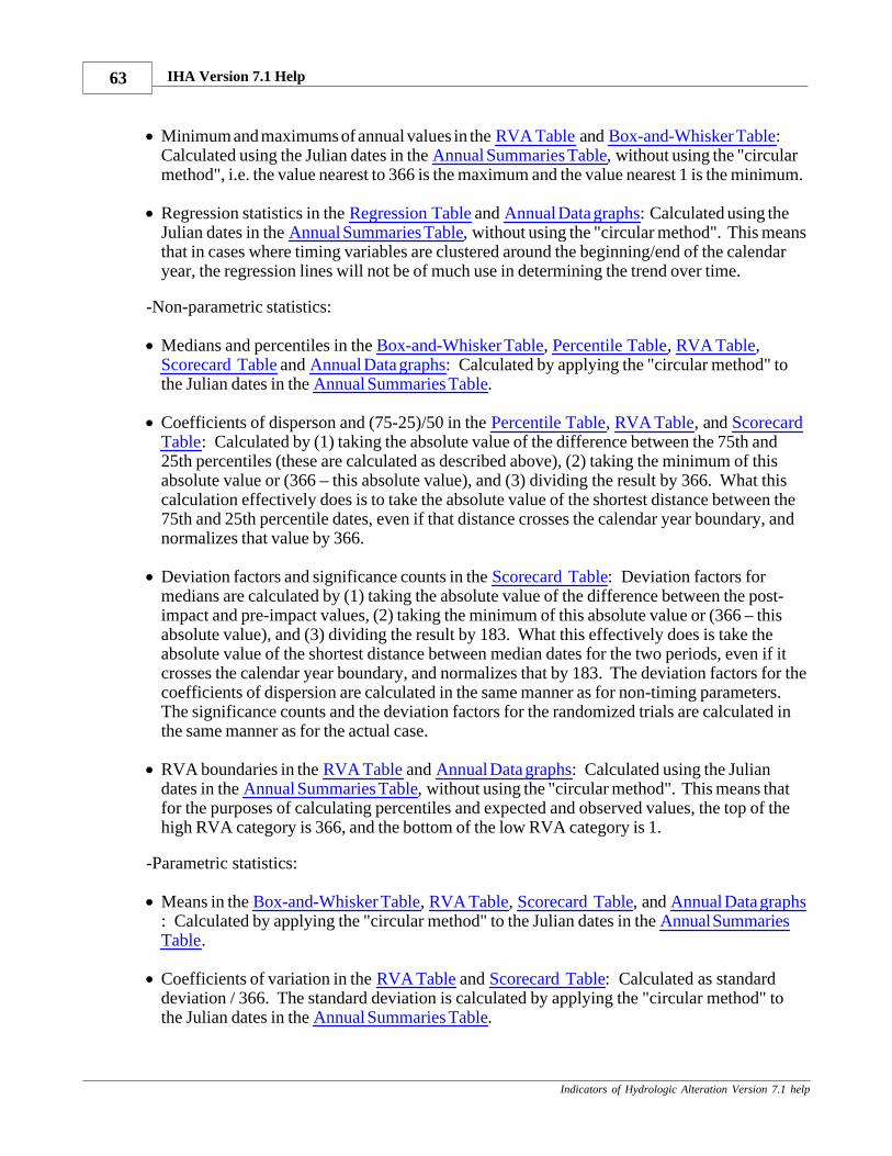
IHA Version 7.1 Help63
Indicators of Hydrologic Alteration Version 7.1 help
· Minimum and maximums of annual values in the RVA Table and Box-and-Whisker Table:Calculated using the Julian dates in the Annual Summaries Table, without using the "circularmethod", i.e. the value nearest to 366 is the maximum and the value nearest 1 is the minimum.
· Regression statistics in the Regression Table and Annual Data graphs: Calculated using theJulian dates in the Annual Summaries Table, without using the "circular method". This meansthat in cases where timing variables are clustered around the beginning/end of the calendaryear, the regression lines will not be of much use in determining the trend over time.
-Non-parametric statistics:
· Medians and percentiles in the Box-and-Whisker Table, Percentile Table, RVA Table,Scorecard Table and Annual Data graphs: Calculated by applying the "circular method" tothe Julian dates in the Annual Summaries Table.
· Coefficients of disperson and (75-25)/50 in the Percentile Table, RVA Table, and ScorecardTable: Calculated by (1) taking the absolute value of the difference between the 75th and25th percentiles (these are calculated as described above), (2) taking the minimum of thisabsolute value or (366 – this absolute value), and (3) dividing the result by 366. What thiscalculation effectively does is to take the absolute value of the shortest distance between the75th and 25th percentile dates, even if that distance crosses the calendar year boundary, andnormalizes that value by 366.
· Deviation factors and significance counts in the Scorecard Table: Deviation factors formedians are calculated by (1) taking the absolute value of the difference between the post-impact and pre-impact values, (2) taking the minimum of this absolute value or (366 – thisabsolute value), and (3) dividing the result by 183. What this effectively does is take theabsolute value of the shortest distance between median dates for the two periods, even if itcrosses the calendar year boundary, and normalizes that by 183. The deviation factors for thecoefficients of dispersion are calculated in the same manner as for non-timing parameters. The significance counts and the deviation factors for the randomized trials are calculated inthe same manner as for the actual case.
· RVA boundaries in the RVA Table and Annual Data graphs: Calculated using the Juliandates in the Annual Summaries Table, without using the "circular method". This means thatfor the purposes of calculating percentiles and expected and observed values, the top of thehigh RVA category is 366, and the bottom of the low RVA category is 1.
-Parametric statistics:
· Means in the Box-and-Whisker Table, RVA Table, Scorecard Table, and Annual Data graphs: Calculated by applying the "circular method" to the Julian dates in the Annual SummariesTable.
· Coefficients of variation in the RVA Table and Scorecard Table: Calculated as standarddeviation / 366. The standard deviation is calculated by applying the "circular method" tothe Julian dates in the Annual Summaries Table.
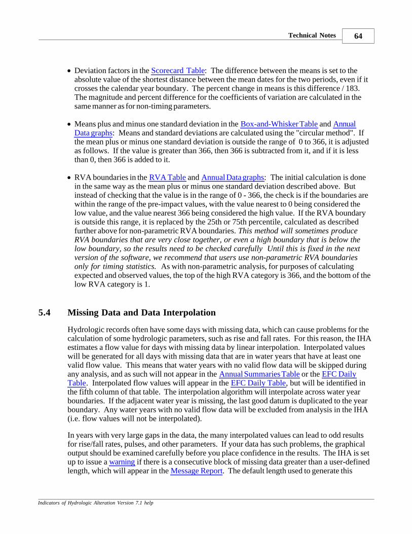
Technical Notes 64
Indicators of Hydrologic Alteration Version 7.1 help
· Deviation factors in the Scorecard Table: The difference between the means is set to theabsolute value of the shortest distance between the mean dates for the two periods, even if itcrosses the calendar year boundary. The percent change in means is this difference / 183. The magnitude and percent difference for the coefficients of variation are calculated in thesame manner as for non-timing parameters.
· Means plus and minus one standard deviation in the Box-and-Whisker Table and AnnualData graphs: Means and standard deviations are calculated using the "circular method". Ifthe mean plus or minus one standard deviation is outside the range of 0 to 366, it is adjustedas follows. If the value is greater than 366, then 366 is subtracted from it, and if it is lessthan 0, then 366 is added to it.
· RVA boundaries in the RVA Table and Annual Data graphs: The initial calculation is donein the same way as the mean plus or minus one standard deviation described above. Butinstead of checking that the value is in the range of 0 - 366, the check is if the boundaries arewithin the range of the pre-impact values, with the value nearest to 0 being considered thelow value, and the value nearest 366 being considered the high value. If the RVA boundaryis outside this range, it is replaced by the 25th or 75th percentile, calculated as describedfurther above for non-parametric RVA boundaries. This method will sometimes produceRVA boundaries that are very close together, or even a high boundary that is below thelow boundary, so the results need to be checked carefully Until this is fixed in the nextversion of the software, we recommend that users use non-parametric RVA boundariesonly for timing statistics. As with non-parametric analysis, for purposes of calculatingexpected and observed values, the top of the high RVA category is 366, and the bottom of thelow RVA category is 1.
5.4 Missing Data and Data Interpolation
Hydrologic records often have some days with missing data, which can cause problems for thecalculation of some hydrologic parameters, such as rise and fall rates. For this reason, the IHAestimates a flow value for days with missing data by linear interpolation. Interpolated valueswill be generated for all days with missing data that are in water years that have at least onevalid flow value. This means that water years with no valid flow data will be skipped duringany analysis, and as such will not appear in the Annual Summaries Table or the EFC DailyTable. Interpolated flow values will appear in the EFC Daily Table, but will be identified inthe fifth column of that table. The interpolation algorithm will interpolate across water yearboundaries. If the adjacent water year is missing, the last good datum is duplicated to the yearboundary. Any water years with no valid flow data will be excluded from analysis in the IHA(i.e. flow values will not be interpolated).
In years with very large gaps in the data, the many interpolated values can lead to odd resultsfor rise/fall rates, pulses, and other parameters. If your data has such problems, the graphicaloutput should be examined carefully before you place confidence in the results. The IHA is setup to issue a warning if there is a consecutive block of missing data greater than a user-definedlength, which will appear in the Message Report. The default length used to generate this
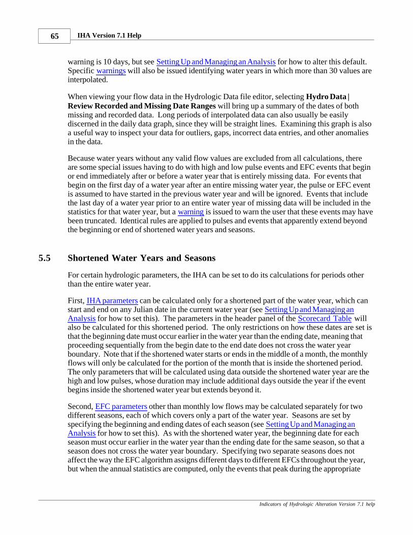
IHA Version 7.1 Help65
Indicators of Hydrologic Alteration Version 7.1 help
warning is 10 days, but see Setting Up and Managing an Analysis for how to alter this default.Specific warnings will also be issued identifying water years in which more than 30 values areinterpolated.
When viewing your flow data in the Hydrologic Data file editor, selecting Hydro Data |Review Recorded and Missing Date Ranges will bring up a summary of the dates of bothmissing and recorded data. Long periods of interpolated data can also usually be easilydiscerned in the daily data graph, since they will be straight lines. Examining this graph is alsoa useful way to inspect your data for outliers, gaps, incorrect data entries, and other anomaliesin the data.
Because water years without any valid flow values are excluded from all calculations, thereare some special issues having to do with high and low pulse events and EFC events that beginor end immediately after or before a water year that is entirely missing data. For events thatbegin on the first day of a water year after an entire missing water year, the pulse or EFC eventis assumed to have started in the previous water year and will be ignored. Events that includethe last day of a water year prior to an entire water year of missing data will be included in thestatistics for that water year, but a warning is issued to warn the user that these events may havebeen truncated. Identical rules are applied to pulses and events that apparently extend beyondthe beginning or end of shortened water years and seasons.
5.5 Shortened Water Years and Seasons
For certain hydrologic parameters, the IHA can be set to do its calculations for periods otherthan the entire water year.
First, IHA parameters can be calculated only for a shortened part of the water year, which canstart and end on any Julian date in the current water year (see Setting Up and Managing anAnalysis for how to set this). The parameters in the header panel of the Scorecard Table willalso be calculated for this shortened period. The only restrictions on how these dates are set isthat the beginning date must occur earlier in the water year than the ending date, meaning thatproceeding sequentially from the begin date to the end date does not cross the water yearboundary. Note that if the shortened water starts or ends in the middle of a month, the monthlyflows will only be calculated for the portion of the month that is inside the shortened period. The only parameters that will be calculated using data outside the shortened water year are thehigh and low pulses, whose duration may include additional days outside the year if the eventbegins inside the shortened water year but extends beyond it.
Second, EFC parameters other than monthly low flows may be calculated separately for twodifferent seasons, each of which covers only a part of the water year. Seasons are set byspecifying the beginning and ending dates of each season (see Setting Up and Managing anAnalysis for how to set this). As with the shortened water year, the beginning date for eachseason must occur earlier in the water year than the ending date for the same season, so that aseason does not cross the water year boundary. Specifying two separate seasons does notaffect the way the EFC algorithm assigns different days to different EFCs throughout the year,but when the annual statistics are computed, only the events that peak during the appropriate
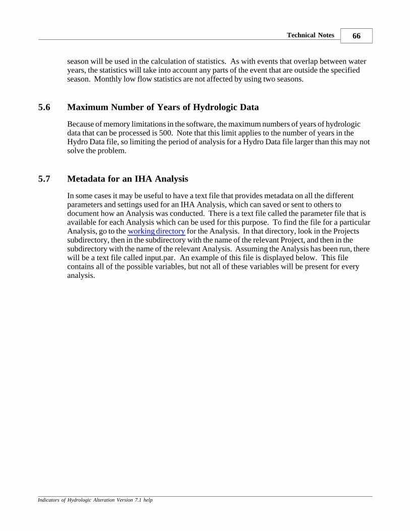
Technical Notes 66
Indicators of Hydrologic Alteration Version 7.1 help
season will be used in the calculation of statistics. As with events that overlap between wateryears, the statistics will take into account any parts of the event that are outside the specifiedseason. Monthly low flow statistics are not affected by using two seasons.
5.6 Maximum Number of Years of Hydrologic Data
Because of memory limitations in the software, the maximum numbers of years of hydrologicdata that can be processed is 500. Note that this limit applies to the number of years in theHydro Data file, so limiting the period of analysis for a Hydro Data file larger than this may notsolve the problem.
5.7 Metadata for an IHA Analysis
In some cases it may be useful to have a text file that provides metadata on all the differentparameters and settings used for an IHA Analysis, which can saved or sent to others todocument how an Analysis was conducted. There is a text file called the parameter file that isavailable for each Analysis which can be used for this purpose. To find the file for a particularAnalysis, go to the working directory for the Analysis. In that directory, look in the Projectssubdirectory, then in the subdirectory with the name of the relevant Project, and then in thesubdirectory with the name of the relevant Analysis. Assuming the Analysis has been run, therewill be a text file called input.par. An example of this file is displayed below. This filecontains all of the possible variables, but not all of these variables will be present for everyanalysis.
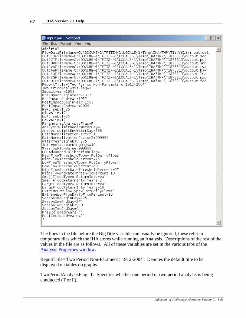
IHA Version 7.1 Help67
Indicators of Hydrologic Alteration Version 7.1 help
The lines in the file before the BigTitle variable can usually be ignored, these refer totemporary files which the IHA stores while running an Analysis. Descriptions of the rest of thevalues in the file are as follows. All of these variables are set in the various tabs of the Analysis Properties window.
ReportTitle='Two Period Non-Parametric 1912-2004': Denotes the default title to bedisplayed on tables on graphs.
TwoPeriodAnalysisFlag=T: Specifies whether one period or two period analysis is beingconducted (T or F).

Technical Notes 68
Indicators of Hydrologic Alteration Version 7.1 help
ImpactYear=1953: The impact year. For two period analysis, this is set to be equal toPostImpactBeginYear.
PreImpactBeginYear=1912: For two period analysis, this is the beginning year of the pre-impact period. For single period analysis, this will be the first year of the period to beanalyzed.
PreImpactEndYear=1952: For two period analysis, this is the end year of the pre-impactperiod. For single period analysis, this will be the last year of the period to be analyzed.
PostImpactBeginYear=1953: For two period analysis, this is the beginning year of the post-impact period.
PostImpactEndYear=2004: For two period analysis, this is the end year of the post-impactperiod.
HiPulseLvl=25: The high pulse threshold, either in percentiles (non-parametric analysis) ornumber of standard deviations (parametric analysis).
HiRVAlim=17: The lower boundary of the high RVA category, either in percentiles (non-parametric analysis) or number of standard deviations (parametric analysis). This will be setbut not used for single period analysis.
LoPulseLvl=25: The low pulse threshold, either in percentiles (non-parametric analysis) ornumber of standard deviations (parametric analysis).
LoRVALim=17: The upper boundary of the low RVA category, either in percentiles (non-parametric analysis) or number of standard deviations (parametric analysis). This will be setbut not used for single period analysis.
ParametricAnalysisFlag=F: Whether parametric (T) or non-parametric analysis (F)
AnalysisLimitBeginWaterDay=1: First day of the water year. This is expressed as the date ofthe water year, and is only different from 1 if a shortened water year is being used for IHAparameters.
AnalysisLimitEndWaterDay=366: Last day of the water year. This is expressed as the date ofthe water year, and is only different from 366 if a shortened water year is being used for IHAparameters.
DataNormalizationFactor=1: Constant by which all flow data in the first Hydro Data file isdivided.
DataNormalizationFactor2=999999: Constant by which all flow data in the second Hydro Datafile is divided (only available for a two Hydro Data file analysis).
WaterYearBeginDay=275: Julian date of the first day of the water year.
IHA Version 7.1 Help69
Indicators of Hydrologic Alteration Version 7.1 help
InterpolateWarningDays=10: Number of days of missing data required to trigger a warningmessage.
MissingFlowValue=999999: Value for no data used in input data file.
EFCAdvancedCalibrationFlag=T: Use advanced calibration method for EFC algorithm (T orF).
HighFlowThresholdType='PctDailyFlows': Method used to specify the high flow threshold inthe EFC algorithm (can be 'PctDailyFlows' or 'FlowRate').
When using 'PctDailyFlows' - HighFlowThresholdPercent=75: Percentile used.When using 'FlowRate' - HighFlowThresholdFlowRate=750: Flow value used.
LowFlowThresholdType='PctDailyFlows' Method used to specify the low flow threshold inthe EFC algorithm (can be 'PctDailyFlows' or 'FlowRate').
When using 'PctDailyFlows' - LowFlowThresholdPercent=60: Percentile used.When using 'FlowRate' - LowFlowThresholdFlowRate=600: Flow value used.
HighFlowStartRateThresholdPercent=25: High flow start rate threshold used in the EFCalgorithm.
HighFlowEndRateThresholdPercent=10: High flow end rate threshold used in the EFCalgorithm.
SmallFloodType='ReturnInterval': Method used to specify the small flood minimum peak flowused in the EFC algorithm (can be 'ReturnInterval', 'Flow Rate', or 'PctDailyFlows').
When using 'ReturnInterval' - SmallFloodReturnIntvlYears=2: Return interval used.When using 'Flow Rate' - SmallFloodFlowRate=2000: Flow rate used.When using 'PctDailyFlows' - SmallFloodPercent=95: Percentile used.
LargeFloodType='ReturnInterval': Method used to specify the large flood minimum peak flowused in the EFC algorithm (can be 'ReturnInterval', 'Flow Rate', or 'PctDailyFlows').
When using 'ReturnInterval' - SmallFloodReturnIntvlYears=10: Return interval used.When using 'Flow Rate' - SmallFloodFlowRate=10000: Flow rate used.When using 'PctDailyFlows' - SmallFloodPercent=98: Percentile used.
ExtremeLowFlowType='PctDailyFlows': Method used to specify the extreme low flowthreshold in the EFC algorithm (can be 'PctDailyFlows', 'PctAllLowFlows', or 'FlowRate').
When using 'PctDailyFlows' - ExtremeLowFlowDailyFlowPercent=10: Percentileused.
When using 'PctAllLowFlows' - ExtremeLowFlowLowFlowsPercent=10: Percentileused.
When using 'FlowRate' - ExtremeLowFlowFlowRate=22: Flow rate used.
Technical Notes 70
Indicators of Hydrologic Alteration Version 7.1 help
SeasonOneBeginDay=275: Julian date of the first day used for EFC calculations. Will only bedifferent from WaterYearBeginDay if two seasons are used for EFC parameters.
SeasonOneEndDay=274: Julian date of the last day used for EFC calculations. Will only bedifferent from WaterYearBeginDay -1 if two seasons are used for EFC parameters.
SeasonTwoBeginDay=0: Julian date of the first day of the EFC second season. Will only bedifferent from 0 if two seasons are used for EFC parameters.
SeasonTwoEndDay=0: Julian date of the last day of the EFC second season. Will only bedifferent from 0 if two seasons are used for EFC parameters.
PreExcludedYears=' ': Years excluded from analysis for purposes of computing Flow DurationCurves for pre-impact period.
PostExcludedYears=' ': Years excluded from analysis for purposes of computing FlowDuration Curves for post-impact period.
5.8 Issues with Large Flow Values
In its internal calculations, the IHA represents no data values with the number 999999. Because of this, it is possible that using the IHA with flow datasets that have flow values in thesame magnitude as this number will yield some calculation errors. So if any daily flows arenear to 1,000,000, the entire flow dataset should be converted to another unit or divided by afactor so that the flow values are smaller.
This issue is a legacy of the FORTRAN code written for early versions of the IHA, and will becorrected in the next version of the software.
5.9 Warning Messages
Below is a description of all the warning messages that may appear in the Message Report.When comparing two Hydro Data files, certain messages may indicate the name of theHydro Data file.
Message: An EFC flood or high flow pulse event has been truncated by missing year 1956.This event is used to compute annual statistics, but its length has been truncated.
Message: An EFC extreme low flow event has been truncated by missing year 1956. Thisevent is used to compute annual statistics, but its length has been truncated.
Message: An EFC flood or high flow pulse event has been truncated at the end of the dataset.This event is used to compute annual statistics, but its length has been truncated.
Message: An EFC extreme low flow event has been truncated at the end of the dataset. Thisevent is used to compute annual statistics, but its length has been truncated.
These messages are to warn the user that the end of an EFC event that is included in the EFC
IHA Version 7.1 Help71
Indicators of Hydrologic Alteration Version 7.1 help
statistics has been truncated by a missing water year of data or by the end of the dataset. Statistics for such events may have errors because part of the event is missing from the flowdataset.
Message: An EFC flood or high flow pulse event has been truncated at the beginning of thedataset. This event is not used to compute annual statistics.
Message: An EFC extreme low flow event has been truncated at the beginning of the dataset.This event is not used to compute annual statistics.
Message: An EFC flood or high flow pulse event has been truncated at the beginning bymissing year 1972. This event is not used to compute annual statistics.
Message: An EFC extreme low flow event has been truncated at the beginning by missing year1972. This event is not used to compute annual statistics.
These messages are to warn the user that an EFC event has been ignored in the annualstatistics because it started on the first day at the beginning of the dataset or on the first dayafter a missing year. Such events are assumed to have started prior to the first day of thewater year (in the previous water year), so our convention is to exclude them from theannual statistics.
Message: A high pulse has been truncated by missing year 1956 Message: A low pulse has been truncated by missing year 1956
This message is to warn the user that the end of a high or low pulse that is included in thestatistics has been truncated by a missing water year of data. Statistics for such events mayhave errors because part of the event is missing from the flow dataset.
Message: Dates of extreme flows are widely distributed throughout the year. Use statisticswith caution.
This message refers to the timing of annual 1-day maximum and minimum flows and EFCevents, and is triggered when the annual data values appear to be widely scatteredthroughout the calendar year. For specifics on when this warning is generated, see the Calculating Statistics for Timing Variables.
Message: The lower RVA limit is outside the range of variability of parameter High pulseduration. The 25th percentile level will be used.
Message: The upper RVA limit is outside the range of variability of parameter Low pulsecount. The 75th percentile level will be used
These messages appear when one of the RVA boundaries is outside the range of the data,and indicate that this value has been replaced with the relevant percentile value.
Message: The parametric low pulse level is <0. It will be replaced by the 25th percentilevalue.
Technical Notes 72
Indicators of Hydrologic Alteration Version 7.1 help
For parametric analysis, this appears when the low pulse level is set at less than 0, andindicates that it has been replaced by the 25th percentile.
Message: There is not enough pre-impact data to calculate RVA limits for parameter April.
This appears in certain situations when RVA boundaries cannot be calculated. This happenswhen there is only one year of pre-impact data, or when there is no post-impact data.
Message: WARNING: Some of the Colwell parameters are based on fewer than twenty yearsof data
This warns the user when the Colwell Parameters (flow predictability, constancy, andcontingency) reported at the beginning of the Scorecard Table are based on fewer than 20years of data.
Message: WARNING: variance of a mean date is > 180 days.
This appears when the standard deviation calculated for a timing statistics is greater than180. For more on when this warning is generated, see the Calculating Statistics for TimingVariables.
Message: 61 daily values have been interpolated in year 1977.
This warning appears for water years where there are numerous days of missing data. Thiswarning only occurs for water years where 30 or more days of data have been interpolated.See Missing Data and Data Interpolation for a description of the procedures used when thereare missing data in the Hydro Data file.
Message: The longest period of missing data is 61 days. Interpolating across this gap maycause anomalies in the statistics. Please use them with caution.
This message reports the longest period of missing data in the Hydro Data file, and appearsgap of missing data longer than the threshold value set in Analysis Title/Options tab of theAnalysis Properties window.
5.10 Bug-Tracking Feature
The IHA has a bug-tracking feature that will help the developers further improve the code in thefuture. In the case of an Access Violation or other problem with the code, a window will popup that gives you the option to email a bug report with some information attached to it that willhelp the software developer diagnose the problem. Before sending the email, it would also beuseful if the user could quickly type in the circumstances that caused the error. Note thatoccasionally this window will pop up in the case of a warning that does not necessarily
IHA Version 7.1 Help73
Indicators of Hydrologic Alteration Version 7.1 help
indicate a bug, in which case you can just ignore it by clicking OK.
5.11 Regional and Language Settings
Because different parts of the world use different characters to denote decimal places (usuallyeither a period or a comma), the IHA software will display numbers according to the WindowsRegional and Language settings for the computer. It is possible to view or change these settingsunder the Windows Control Panel, under Regional Language Options. When importing datafrom a text file, the IHA will also expect decimal places to be denoted according to these samesettings. But note that if the language settings are set to denote decimal places as commas,comma-delimited text files will not import properly.
Version 7.1 has a Spanish language help system and user manual. The IHA will automaticallyuse the English language help system unless the user's computer has Spanish language settings. The language choice can also be set manually using the menu option Options -> Set Language.
Future versions of the IHA will have a Chinese language help system and manual, and alsohave an option to switch the language used on all software windows to either Spanish orChinese.
5.12 DOS Command Line Start-Up
The IHA can be started up from the DOS prompt by typing iha7.exe on the command line whenlocated in directory where the IHA is installed. The file IHA7.exe must be present in thedirectory for this to work. IHA can also switch working directories and open up a specificproject when started from the DOS prompt.
There are two options available when using command line startup:
WorkDir= This sets the IHA working directory. If not specified, IHA will open in thesame working directory that was in use the last time the software was used.
Proj= This tells IHA to open up a specific project after it starts, which has to belocated in the working directory as specified above.
An example of use of both of these options is below:
IHA7.exe WorkDir=c:\mynewtestsub Proj="EAST BRANCH"
Double quotes are necessary when there are spaces in the name of the working directory orproject.
Endnotes 74
Indicators of Hydrologic Alteration Version 7.1 help
6 Endnotes
Colwell, R.K. 1974. Predictability, constancy and contingency of periodic phenomena. Ecology 55: 1148-1153.
Huh, S., D.A. Dickey, M.R. Meador and K.E. Ruhl. 2005. Temporal analysis of the frequencyand duration of low and high streamflow: years of record needed to characterize streamflowvariability. Journal of Hydrology 310: 78-94.
Olden, J.D. and N.L. Poff. 2003. Redundancy and the choice of hydrologic indices forcharacterizing streamflow regimes. River Research and Applications (19) 2: 101-121.
Poff, N. L. and J. V. Ward. 1989. Implications of Streamflow Variability and Predictibility forIotic Community Structure: a Regional Analysis of Streamflow Patterns. Canadian Journal ofAquatic Sciences 46: 1805-1818.
Richter, B.D., J.V. Baumgartner, J. Powell, and D.P. Braun. 1996. A method for assessinghydrologic alteration within ecosystems. Conservation Biology 10:1163-1174.
Richter, B.D, J.V. Baumgartner, R. Wigington, and D.P. Braun. 1997. How much water does ariver need? Freshwater Biology 37, 231-249.
Richter, B.D., J.V. Baumgartner, D.P. Braun , and J. Powell, 1998, A Spatial Assessment ofHydrologic Alteration Within a River Network. Regul. Rivers: Res. Mgmt. 14: 329-340.
Taylor, V., G. Jewitt, and R. Schulze. Unpublished. Indicators of Hydrologic Alteration forAssessing Environmental Flows for Highly Variable River.
IHA Version 7.1 Help75
Indicators of Hydrologic Alteration Version 7.1 help
Index
- A -
Analysis set up 5, 6, 15, 21, 22, 24, 26, 33
Analysis years 35
Annual data graphs 56
Annual summaries table 48, 50
Army Corps of Engineers flow data 29
- B -
Base flow 6
Batch processing 30
Box-and-whisker table 48, 54
- C -
Coefficient of dispersion 51
Coefficient of variation 51
Colwell parameters 51
Command line operation 73
Cubic feet per second 32
Cubic meters per second 32
- D -
Daily data graph 56
Deviation factor 51
DOS command line operation 73
Duration 6, 12
- E -
EFC algorithm 15, 21
EFC daily table 48, 55
EFC parameters 1, 5, 10, 12, 15, 21, 48, 55, 56
Environmental Flow Components 1, 5, 10, 12, 15, 21,37, 39, 55, 56
Excel 1, 45, 61
Extreme low flows 10, 12, 15, 21
Extreme water conditions 6
- F -
Fall rates 6, 12
FDC table 55
Floods 10, 12, 15, 21, 51
Flow data 1, 3, 26, 28, 29, 30, 55, 56
Flow duration curves 1, 5, 24, 40, 55, 56
Flow rate units 32
- G -
Graph default settings 44, 57
Graphs 1, 5, 44, 48, 56, 57
- H -
HEC-DSS database files 29
High flow pulses 10, 12, 15, 21
High pulses 6, 38
Hydro Data file 28, 29, 30, 31, 32, 40, 47, 66
Hydrologic Alteration 22, 53, 56
Hydrologic Alteration graph 22, 56
Hydrologic data 1, 3, 26, 28, 29, 30, 55, 56
Hydrologic parameters 6, 10, 12
- I -
IHA parameters 5, 6, 51, 53, 56
Impact year 35
Interpolated data 55, 64
- J -
Julian dates 6, 12, 15, 37, 45, 61
- L -
Language settings 73
Large floods 10, 12, 15, 21
Leap years 61
Least-squares fit line 54, 56
Logarithmic scale 57
Low flows 10, 12, 15, 21
Low pulses 6, 38
Index 76
Indicators of Hydrologic Alteration Version 7.1 help
- M -
Maximum flows 6
Mean 51, 56
Median 51, 56
Message report 35, 48, 55
Metadata 66
Microsoft Excel 1, 45, 61
Minimum flows 6
Missing data 28, 64
Monthly averages graph 22, 56
Monthly flows 6, 56
Monthly low flows 10, 12, 15, 21
- N -
Non-parametric statistics 5, 38, 48, 51, 54, 56
- O -
One period analysis 5, 35, 48, 51, 54, 56
Operating systems 2
- P -
Parametric statistics 5, 38, 48, 51, 56
Peak flow 12
Percentile 54
Percentile table 48, 54
Percentiles 38, 39, 51, 56, 61
Post-impact period 35, 51, 53
Pre-impact period 35, 51, 53
Project 31, 47
Pulse thresholds 6, 38
- R -
Range of Variability Approach 5, 22, 38, 53
Regression parameters 54, 56
Regression table 48, 54
Reversals 6
Rise rates 6, 12
Run analysis 40
RVA analysis 5, 22, 38, 53, 56
RVA category boundaries 38, 56
RVA table 22, 38, 48, 53
- S -
Scorecard table 35, 38, 48, 51
Seasons 5, 10, 12, 21, 37, 48, 65
Shortened water year 5, 6, 37, 38, 65
Significance count 51
Single period analysis 5, 35, 48, 51, 54, 56
Small floods 10, 12, 15, 21
Spreadsheets 1, 45, 48
Standard deviation 51, 56
Statistics 5, 38, 51
System requirements 2
- T -
Tables 1, 5, 48
Technical notes 61
Timing 6, 12
Two Hydro Data file comparison 1, 5, 31, 32, 35
Two period analysis 5, 35, 37, 48, 51, 53, 56
- U -
U.S. Geological Survey 3, 26
USGS 3, 26
- V -
Variance lines 56
View results 33, 48
- W -
Warnings 35, 38, 48, 61, 70
Water Survey of Canada data 29
Water year 5, 6, 12, 15, 32, 35, 37, 45, 65
Watershed area 35, 51
Wizard 33
Working directory 47
- Z -
Zero flow days 6