Incomplete Risk Sharing and Monetary Policy in a Small

Open Economy�

Jaime Alonso-Carrera† and Timothy Kam∗

ABSTRACT

We propose an alternative and simple small open economy model with incomplete interna-tional asset markets. This model allows us to analytically dissect the role of market incom-pleteness in a small open economy model of monetary policy. Our model nests the canoni-cal two-equation closed economy and the complete-markets small open economy as specialcases. In constrast to existing models, we show that asset market incompleteness resultsin the real exchange rate being an explicit, or irreducible, variable in the equilibrium char-acterization. Moreover, this explicit equilibrium exchange rate channel has an endogenous“cost-push” monetary-policy trade-off interpretation. This provides an alternative meansof breaking the “monetary-policy isomorphism” between the small open economy and itsclosed economy limit. We then show that established lessons on local stability of rational ex-pectations equilibrium under alternative monetary policies are reversed when the economycannot completely insure country-specific risks.

JEL CODES: E52; F41KEYWORDS: Incomplete Markets; Monetary Policy Isomorphism;

Exchange Rate; Equilibrium Determinacy

†Departamento de Fundamentos del Analisis Economico & RGEAUniversidade de VigoCampus As Lagoas-Marcosende36310 Vigo, SpainEmail: jalonso@uvigo.es†

∗School of EconomicsH.W. Arndt Building 25aThe Australian National UniversityA.C.T. 0200, AustraliaE-mail: timothy.kam@anu.edu.au∗

� J. Alonso-Carrera thanks the School of Economics and CAMA at the Australian National University for their hospitality during a visitwhere this paper was written. Financial support from the Spanish Ministry of Science and FEDER through grant ECO2008-02752; from theSpanish Ministry of Education through grant PR2009-0162; from Xunta de Galicia through grant 10PXIB30001777PR; from the Generalitatde Catalunya through grant SGR2009-1051; from EDN program funded by Australian Research Council; and from CAMA at AustralianNational University are gratefully acknowledged. T. Kam thanks RGEA at Universidade de Vigo for funding support and their hospitality.We thank Craig Burnside, V.V. Chari, Richard Dennis, Mark Gertler, Simon Gilchrist, Bruce Preston, Christoph Thoenissen and Tao Zhafor useful suggestions and beneficial conversations. This paper evolved from an earlier version prepared for the Northwestern CIED andRBNZ Monetary Policy Conference, “Twenty Years of Inflation Targeting” held in Wellington in December 2009.

1 Introduction

Why should small open economy monetary authorities care about international exchange rates?Is there a justification for managing exchange rates, and what is its connection to incomplete in-ternational risk sharing of country-specific shocks? In practice, in many small open economieswith floating exchange rate regimes, the dynamics of the exchange rate matter, in structuralmodelling, and for monetary policy design. Also it remains unclear in the literature, whichmonetary policy can induce equilibrium stability, when the dynamics of the exchange rate can-not be decoupled from inflation and output gap in an equilibrium characterization.

In standard monetary-policy small open economy models, the exchange rate is a reduciblevariable in equilibrium. In other words, its explicit dynamics can be decoupled from neces-sary equilibrium conditions. Specifically, under certain restrictions on inter- and intra-temporalelasticities of substitution, the open economy dimension merely alters the equilibrium condi-tions that are familiar to a closed economy model in terms of the slopes of an IS curve and aPhillips curve [see Benigno and Benigno, 2003; Galı and Monacelli, 2005; Clarida et al., 2001].More generally, if these parametric restrictions are relaxed, Benigno and Benigno [2003] haveshown that the monetary policy implication for the open economy is no longer isomorphic toits closed-economy limit. That is, the design of monetary policy for the small open economymust also take into account the trade-offs arising from the open economy channels. However,the explicit dynamics of the exchange rate is still redundant in these systems as long as theopen economy has access to a complete international state-contingent asset market.

We propose an alternative and tractable small open economy model with incomplete inter-national asset markets in order to address these two questions. Our model nests the canonicalcomplete-markets small open economy model of Galı and Monacelli [2005] and the standardNew Keynesian closed economy model [see e.g. Woodford, 2003] as special cases. Our contri-bution is two-fold.

First, incomplete markets result in an irreducible and explicit exchange rate channel, in themodel’s equilibrium characterization. This result introduces a truly endogenous “cost-push”trade-off for monetary policy, in the sense that this “cost-push” term is itself an irreducible en-dogenous variable. This is in contrast to complete-markets small open economy models, wherethe reducible exchange-rate channel merely creates a “cost-push” trade-off in terms of exoge-nous factors such as foreign output gap. We also show that the irreducibility of the exchangerate and cost-push trade-off depends solely on an assumption of incomplete international as-set markets.1 As a corollary, we also obtain a break in the “monetary-policy isomorphism”between the small open economy and its closed economy limit.

Second, we show that established lessons on local stability of rational expectations equilibrium(REE) under alternative monetary policies are reversed as a result of the fact that the economycannot completely insure country-specific risks completely. The latter poses additional restric-tions on the admissibility of policy rules in inducing determinate REE. We show that while the

1Our general model admits two other sources through which the exchange rate may explicitly matter: (i) Theinteraction between endogenous discounting—which is required to induce a unique steady state [see Schmitt-Groheand Uribe, 2003] —and intra-temporal substitution between home- and foreign-produced final consumption goods;and (ii) The possibility of an imported input in the small economy’s production structure. We show that in the limitwhen these two sources are removed, an irreducible exchange rate dynamics still remains; and this is purely a resultfrom the existence of incomplete international asset markets.

2

inability of a small open economy to insure its country-specific technology risk reduces suchadmissible sets of monetary policies, it can be improved by a family of simple policies that takeinto account exchange rate growth as well.

We provide a simple theoretical foundation for standard monetary policy modelling andpractice in small open economies with floating exchange rates. In practice, modellers and poli-cymakers in these economies take into account explicit exchange rate dynamics, in model equi-librium conditions, and, also in policy objectives. For example, clause 4(b) of New Zealand’s2002 Policy Targets Agreement states that:2

“[I]n pursuing its price stability objective, the Bank shall seek to avoid unnecessaryinstability in output, interest rates and the exchange rate”.

There are existing departures from the “isomorphism” result, in the sense that the exchangerate is irreducible from equilibrium characterization. A seminal departure is Monacelli [2005],who assumes complete asset markets and sticky prices in the imported goods sector. The lat-ter creates a short-run law of one price gap, and therefore imperfect pass through of the ex-change rate to domestic prices. This mechanism results in an endogenous cost-push shockto the Phillips curve. de Paoli [2009b] also considers a small open economy with incompletemarkets. de Paoli [2009b] ensures the existence of a well-defined steady state by introducingportfolio adjustment cost for trade in the non-state-contingent money claims. de Paoli [2009b]focuses on business cycle and welfare properties of her model with international asset-marketincompleteness. In contrast, by assuming negligibly small endogenous discounting of futurepayoffs of agents in our model, we are able to have a more tractable model and we explicitlycharacterize the channels that deliver our endogenous monetary-policy trade-off. Moreover,we do not require additional price-stickiness assumptions on imported goods as in Monacelli[2005], in order to deliver irreducible exchange rate dynamics in equilibrium.

Our analysis in this paper also complements existing two-country open economy modelswith incomplete asset markets. For example, Corsetti et al. [2010] show that international assetmarket incompleteness restrict open economies in achieving efficient consumption allocations,regardless of the existence of price flexibility. However, the issue of closing the small open econ-omy with incomplete markets is also important, and this is a non-issue in large two-countrymodels. Moreover, the role of international asset market incompleteness in affecting REE determi-nacy or indeterminacy under alternative monetary-policy rules have not been studied, in eitherthe two-country or small open economy environments. This paper deals with these issues forthe small open economy case.

Therefore, our contribution is to fill a gap in the literature by providing a tractable version ofa small-open economy model whose equilibrium characterization, allows for a careful dissectionof the role of incomplete markets in delivering an endogenous output-gap-inflation trade off.Moreover, our application provides a complementary exercise, with respect to open-economymodels with incomplete markets [e.g. de Paoli, 2009b; Corsetti et al., 2010], by revisiting andcontrasting with well-known results [e.g. Bullard and Mitra, 2002; Llosa and Tuesta, 2008] interms of indeterminacy of REE vis-a-vis standard simple monetary policy rules.

2The Reserve Bank of New Zealand pioneered inflation targeting, implementing this policy in 1990.

3

The rest of the paper is organized as follows. In Section 2, we describe the details of ouralternative model. Then we characterize competitive equilibrium in Section 3 and explain theeffect of how asset market incompleteness in our model results in an endogenous monetarypolicy trade off in Section 3.3. We then parametrize the model in Section 4. Here we will dis-cuss the implication of market incompleteness on the reduced-form parameters describing theequilibrium trade offs. In Section 5, we analyze the implications of market incompleteness—and therefore the additional restrictions on stability-inducing monetary policy rules—on equi-librium determinacy. Finally in Section 6, we conclude.

2 Model

We propose a small open-economy model consisting of monopolistically competitive domes-tic goods markets with nominal pricing rigidity, and, households that only have access to arestricted set of internationally traded non-state-contingent assets – viz. the incomplete in-ternational asset markets assumption. The domestic economy is small in the sense that localequilibrium outcomes here do not have any impact on the rest of the world, but, the converseis not true. The foreign economy (or the rest of the world) is treated as a large closed economy.We will use variables with an asterisked superscript (e.g. X∗) to refer to the foreign countryand variables without an asterisk to denote the small domestic economy. Subscripts “H” (forHome) and “F” (for Foreign) on certain variables will denote the country of origin for quantitiesand their supporting prices.

A special case of our model is a version of the complete-markets model similar in form toGalı and Monacelli [2005] or Clarida et al. [2001]. The notion of trade openness in our modeladmits: (i) imports of intermediate inputs for producing a final good in the small economy,along the lines of McCallum and Nelson [1999] and Chari et al. [2002]; and (ii) trade in the finaldifferentiated goods. If we shut down these open-economy features in our model, we will alsoobtain the familiar limit of the two-equation closed economy New-Keynesian model similar tothat discussed in Woodford [2003].

2.1 Representative household

As in McCallum and Nelson [1999] or Benigno and Thoenissen [2008], individuals in our smallopen-economy have access only to a pair of domestic and foreign nominal uncontingent bondsdenominated in their own currencies, respectively, Bt and B∗

t . More precisely, let ht := (z0, ..., zt)

denote the t-history of aggregate shocks, where zt = (At, Y∗t ) is a vector of domestic produc-

tivity and foreign output levels, respectively. Bt+1�ht� or B∗

t+1�ht� denotes a claim on one unit

of currency following ht, and is independent of any continuation state zt+1 that may occur att + 1. Let St

�ht� denote the nominal exchange rate, defined as the domestic currency price of

a unit of foreign currency. In domestic currency terms, the prices of one unit of the nominalbonds Bt+1

�ht� and B∗

t+1�ht� are, respectively, 1/[1 + rt

�ht�] and St

�ht� /[1 + r∗t

�ht�], where

rt and r∗t are the respective domestic and the foreign nominal interest rates.The representative consumer in the domestic country faces the following sequential budget

4

constraint, for each t ∈ N, and each (measurable) history ht,

Pt�ht�Ct

�ht�+

Bt+1�ht�

1 + rt (ht)+

St�ht� B∗

t+1�ht�

1 + r∗t (ht)

≤ Wt�ht� Nt

�ht�+ Bt(ht−1) + St

�ht� B∗

t (ht−1) + Πt

�ht� , (2.1)

where Pt is the domestic consumer price indexes, Ct is a composite consumption index, Wt isthe nominal wage rate, Nt denotes the hours of labor supplied, and, Πt is the total nominaldividends received by the consumer from holding equal shares of the domestic firms.

A minor difference of our model to Galı and Monacelli [2005] and McCallum and Nelson[1999] is that consumers exhibit an endogenous discount factor that we denote by ρt. This as-sumption is introduced in order to ensure a unique nonstochastic steady-state consumptionlevel, following Schmitt-Grohe and Uribe [2003].3 However, this is not a fundamental as-sumption for our conclusions with respect to the endogenous monetary-policy trade off arisingfrom the real-exchange-rate channel.4 The consumers’ preferences are given by the followingpresent-value total expected utility function:

E0

�∞

∑t=0

ρt�

U�Ct

�ht��− V

�Nt

�ht���

�, ρt =

β�Ca

t−1(ht−1)

�ρt−1 for t > 0

1 for t = 0, (2.2)

where E0 denotes the expectations operator conditional on time-0 information, and, Cat de-

notes the cross-economy average level of consumption. For concreteness, we will consider thefollowing parametric form for the function β : R+ → (0, 1), following Ferrero et al. [2007]:

β(Cat ) =

β

1 + φ (ln Cat − ϑ)

; β ∈ (0, 1). (2.3)

We do not impose a priori any condition on the sign of the dependence of the discount factoron average consumption, i.e., we only assume that β�(Ca

t ) �= 0. We also assume that per-periodutility of consumption and labor have the respective forms: U

�Ct

�ht�� = Ct

�ht�1−σ /(1 − σ),

and, V�Nt

�ht�� = ψNt

�ht�1+ϕ /(1 + ϕ), where σ > 0, ϕ > 0, and ψ > 0.

The household chooses an optimal plan {Ct(ht), Nt(ht), Bt+1(ht), B∗t+1(h

t)}t∈N to maximize(2.2) subject to (2.1). Unilaterally, the household will take the aggregate outcome Ca

t�ht�, nom-

inal prices {Wt�ht� , Pt

�ht� , St

�ht�}t∈N and policy {rt

�ht�}t∈N as fixed for each measurable

ht, B0(h0) and B∗0(h

0) are known. Denote a measurable selection as Xt�ht� =: Xt. Define the

real exchange rate as Qt := StP∗t /Pt. Given the functional forms, the respective first order

3Galı and Monacelli [2005] assume the existence of an international market for complete state-contingent claims.In doing so, they thus avoid the problem of steady-state allocations being dependent on initial conditions. McCal-lum and Nelson [1999] assume incomplete markets which would mean the opposite for steady state consumption;but this issue is not discussed by the authors.

4Other ways of closing open-economy models are also discussed in Schmitt-Grohe and Uribe [2003]. In ourframework the most natural alternative could be to assume endogenous transaction cost in taking position in foreignbonds (see, e.g., Benigno and Thoenissen [2008]). The model with this alternative assumption would be analyticallyless tractable, and the equilibrium dynamics requires a specific law of motion for bonds. Our assumption willmake clear that what is crucial for the policy trade off is just the incompleteness of financial markets, and not therandom walk property of the asset/consumption dynamics implied by this incompleteness (in the absence of theendogenous discounting assumption).

5

conditions of the household’s problem, for each ht and t ∈ N, are:

ψNϕt Cσ

t =Wt

Pt, (2.4)

C−σt = (1 + rt)Et

�β (Ca

t )

�Pt

Pt+1

�C−σ

t+1

�, (2.5)

C−σt = (1 + r∗t )Et

�β (Ca

t )

�P∗

t Qt+1

P∗t+1Qt

�C−σ

t+1

�. (2.6)

Each optimally chosen Ct will be consistent with the household’s intra-period choice of ahome-produced final consumption good, CH,t and an imported final good CF,t, where Ct isdefined by a CES aggregator

Ct =

�(1 − γ)

1η (CH,t)

η−1η + γ

1η (CF,t)

η−1η

� ηη−1

; γ ∈ (0, 1), η > 1. (2.7)

Furthermore, each type of final good, CH,t and CF,t, are aggregates of a variety of differentiated

goods indexed by i, j ∈ [0, 1]. Respectively, these aggregates are CH,t =�� 1

0 CH,t (i)ε−1

ε di� ε

ε−1 ,

and CF,t =�� 1

0 CF,t (j)ε−1

ε dj� ε

ε−1 , where ε > 1. As is well known from Galı and Monacelli[2005], optimal allocation of the household expenditure across each good type gives rise tostatic demand functions for (CH(i), CF(i), CH, CF) and price indexes. Details of these demandfunctions and prices are given in a supplementary appendix.5

2.2 Differentiated goods technology and pricing

Each domestic firm i ∈ [0, 1] produces a differentiated good. Production is represented by aCES technology

Yt�i, ht� =

�α�

AtNdt�i, ht�

�ν+ (1 − α)

�IMt

�i, ht��ν

� 1ν

; α ∈ (0, 1],−∞ ≤ ν ≤ 1, (2.8)

where Nt(i) is labor hired by the firm and IMt(i) is an index of imported intermediate goods.6

The random variable At := exp{at} is an exogenous embodied labor productivity; α ∈ (0, 1]measures the productive dependence of the domestic economy; and 1/(1 − ν) is the elasticityof substitution between labor and the imported intermediate good. The law of one price andthe limiting closed-economy assumption for the rest of the world ensures that the price of IMt

is equal to StP∗t .

The production cost-minimization problem for the firm is:

min Pt�ht�

�Qt

�ht� IMt

�i, ht�+

Wt�ht�

Pt (ht)Nd

t�i, ht�

�.

5See Supplementary Appendix A.6This intermediate good can be interpreted as two equivalent forms. On the one hand, we can assume that

the imported goods can be either devoted to consumption CF,t or used as a production input IMt. On the otherhand, we can assume that the domestic economy imports two differentiated goods: consumption goods CF,t andintermediated goods IMt.

6

With a homogeneous of degree one production function, the first-order conditions can be writ-ten in the aggregate as

Wt�ht�

Pt (ht)= α

MCnt�ht�

Pt (ht)Aν

t

�Yt

�ht�

Ndt (ht)

�1−ν

(2.9)

and

Qt�ht� = (1 − α)

MCnt�ht�

Pt (ht)

�Yt

�ht�

IMt (ht)

�1−ν

, (2.10)

where MCnt is nominal marginal cost.

Since the firm i ∈ [0, 1] is assumed to be imperfectly competitive, it gets to set an optimalprice PH,t(i, ht) given a Calvo-style random time-independent signal to do so. With a per-periodprobability (1− θ) the firm gets to reset price. As this is quite a standard model in the literature,we derive the details separately (see Supplementary Appendix B). The firm’s optimal pricingdecision is characterized by the first-order condition:

Et

�∞

∑k=0

θk

�t+k−1

∏τ=t

β(Caτ)

�ξt+kξt

Yt+k(i)�

PH,t(i)−�

ε

ε − 1

�MCn

t+k

��= 0, (2.11)

where ξt := UC(Ct), and the demand faced by the firm at some time t + k (and followinghistory ht+k), conditional on the firm maintaining a sale price of PH,t(i) is

Yt+k(i) =�

PH,t(i)PH,t+k

�−ε �CH,t+k + C∗

H,t+k�

. (2.12)

In a symmetric pricing equilibrium, where PH,t := PH,t(ht) = PH,t(i, ht), the law of motion for

the aggregate price is PH,t =�θP1−ε

H,t−1 + (1 − θ)P1−εH,t

� 11−ε .

2.3 Market clearing

In a competitive equilibrium we require that given monetary policy and exogenous processes,the decisions of households and firms are optimal, as characterized earlier, and that marketsclear. First, the labor market must clear, so that (2.4) equals (2.9) for all states and dates. Second,the final Home-produced goods market for each variety i ∈ [0, 1] clears so that:

Yt(i, ht) = CH,t(i, ht) + C∗H,t(i, ht). (2.13)

Third, the no-arbitrage condition for international bonds will be given by the equality of (2.5)and (2.6). In the rest of the world, assumed to be the limiting case of a closed economy, we havemarket clearing as Y∗

t = C∗t .

7

3 Local equilibrium dynamics

In this section we characterize the log-linearized equilibrium dynamics of our small open-economy. To this end, consider the gaps of the aggregate variables with respect to their po-tential level in an equilibrium with fully flexible domestic prices – i.e. when the percentagedeviation (from steady state) of real marginal cost, denoted by mct, is zero at any time t andin any state. Let lowercase variables denote the percentage deviation of its level X from itsnonstochastic steady state point Xss, e.g. x := ln(X/Xss). Define the potential output and thereal exchange rate, respectively, yt and qt, as the levels of output and real exchange rate, respec-tively, at the flexible-price equilibrium. It can be shown that the levels of both yt and qt onlydepend on exogenous variables. Let �xt and �qt denote the domestic output gap and the realexchange rate gap (in percentage deviation), respectively, where �xt = yt − yt and �qt = qt − qt.It can be shown that the equilibrium dynamics can be fully approximated to first-order accu-racy as a system of stochastic dynamic equations for �xt, πH,t and �qt. (Detailed derivations areprovided in Section C of an appendix available separately.)

Definition 1 Given a monetary policy process {rt}t∈N and exogenous processes {�t, ut}t∈N, a rationalexpectations competitive equilibrium is a bounded stochastic process {πH,t, �xt, �qt}t∈N satisfying:

πH,t = βEt {πH,t+1}+ λ (κ1�xt + κ2�qt) , (3.1)

�xt = �Et {�xt+1}− µ [rt − Et {πH,t+1}] + χEt {�qt+1}+ �t, (3.2)

�qt = Et {�qt+1}− (1 − γ) [rt − Et {πH,t+1}] + ut. (3.3)

where

λ =(1 − ν)(1 − δ)

1 − ν + δϕ

�(1 − θ)

�1 − θβ

�

θ

�,

κ1 = ϕ +σ

1 − γ, κ2 =

δ(1 − ν + ϕ)(1 − γ)(1 − ν)(1 − δ)

− σηγ(2 − γ)

(1 − γ)2 +γ

(1 − γ);

� =σ

σ − φ, µ =

�1 − γ

σ − φ

� �1 − γ +

ηγ (2 − γ) (σ − φ)1 − γ

�, χ =

ηγφ (2 − γ)(1 − γ) (σ − φ)

;

δ = (1− α)(IMss/Yss)ν, with IMss and Yss as the stationary values of imported intermediate good andaggregate output, respectively.

3.1 Discussion: Irreducible equilibrium exchange rate dynamics

Consider the equilibrium IS functional equation (3.2). In our small open economy the realexchange rate indirectly affects the output gap via the ex-ante real interest rate (through µ). Thisindirect channel is similar to the standard models of Galı and Monacelli [2005] and Claridaet al. [2001], and, depends on the degree of openness γ.7 Note however, movements in the

7The depreciation in the real exchange rate raises the consumer price index because: (i) it increases the priceof the imported consumption goods; and (ii) increases export demand, which results into a rise in the price ofdomestically produced goods. This increase in the consumer price index reduces the expected rate of inflationfor a given expected future price level. This leads to an increase in the real interest rate facing consumers and,

8

conditional expectation of the real exchange rate in our model also affect the output gap (via χ)directly: (i) by modifying the marginal rate of substitution of consumption between differentperiods and across states (i.e. φ); and (ii) the interaction of these effects with the substitutionbetween home and foreign-produced good (via η). This direct channel is just an artefact of theendogenous discount rate model, and, is negligible when we assume the limiting case for theelasticity of the discount rate with respect to aggregate consumption, φ � 0. In this case, χ ≈ 0.This assumption merely follows Ferrero et al. [2007].8

Equation (3.1) is an augmented New Keynesian Phillips curve representing the dynamicsof the short-run aggregate supply. In contrast to the standard model [e.g. Clarida et al., 2001;de Paoli, 2009a], we do not need to assume exogenous ”cost-push shocks” in order to create anon-trivial monetary policy trade-off.9 The relevant monetary-policy trade-offs embedded inthe Phillips curve, between �xt and πH,t, is now driven by this endogenous “cost-push” chan-nel (via λκ2).10 In our model, the direct link between real exchange rate movements and thereal marginal cost can be dissected into two effects: production and demand channels. Thesefurther correspond to the three terms in the composite parameter κ2 in equation (3.1). First,we have the channel on the production side (i.e. the first term in κ2). Exchange rate depreci-ation in our model increases the unit price of the imported intermediate good, which drivesthe marginal cost and therefore domestic goods inflation up. Second, on the demand side, anincrease in the real exchange rate (or an exchange rate depreciation) increases the prices of theimported consumption goods faced by domestic consumers. This effect has a substitution andan income effect on the marginal cost and the domestic inflation. On the one hand (i.e. thesecond term in κ2), this increase in the price of imported consumption goods leads consumersto reduce the demand of these goods and therefore to reduce aggregate consumption and toincrease leisure. This translates into an increase in marginal product of labor that drives themarginal cost up. On the other hand (i.e. the third term in κ2), this increase in the price ofimported consumption goods reduces the real wage rate facing by consumers, who react byincreasing labor supply to compensate the reduction in the purchasing power of their givenincome. This leads to a reduction in marginal product of labor that pushes the marginal costdown. Observe that the substitution effect dominates, so that the net effect of the increase inthe price of the imported consumption goods on marginal cost is always negative.

Therefore, the overall impact of the real exchange rate on the domestic inflation (i.e., thesign of κ2) is then ambiguous, and it depends on the degree of openness γ and the productivedependence α (through their effect on δ). For empirically plausible parametrization, we show,in Section 4.1, that the overall sign of this slope λκ2 is negative.

Finally, note that our general model admits two other sources through which the exchange

therefore, a decrease in consumption and output for a given expectation of the future exchange rate. Note however,the productive dependence given by δ does not affect the sensitivity of output gap to changes in real exchange ratebecause this parameter only determines the supply-side channel.

8Furthermore, φ, affects the elasticities of output gap with respect to the ex-ante real interest rate µ. Again, withφ � 0, this indirect channel introduced by endogenous discounting will be negligible.

9 See Clarida et al. [1999] for a detailed discussion on this ad-hoc cost-push term.10In our model the real marginal cost is not fully tied to the output gap but also depends on the real exchange

rate as is shown in Section C of the supplementary appendix. Moreover, as (3.3) shows, the dynamics of the realexchange rate depends on the exogenous variable ut for an the endogenous nominal interest rate rt policy outcome.This feature of our model does not rely on price stickiness in an additional imported goods sector as in Monacelli[2005].

9

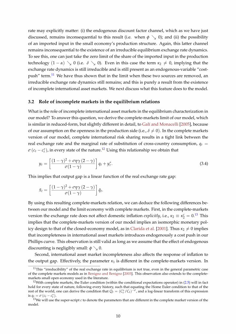
rate may explicitly matter: (i) the endogenous discount factor channel, which as we have justdiscussed, remains inconsequential to this result (i.e. when φ � 0); and (ii) the possibilityof an imported input in the small economy’s production structure. Again, this latter channelremains inconsequential to the existence of an irreducible equilibrium exchange rate dynamics.To see this, one can just take the zero limit of the share of the imported input in the productiontechnology (1 − α) � 0 (i.e. δ � 0). Even in this case the term κ2 �= 0, implying that theexchange rate dynamics is still irreducible and is still present as an endogenous-variable “cost-push” term.11 We have thus shown that in the limit when these two sources are removed, anirreducible exchange rate dynamics still remains; and this is purely a result from the existenceof incomplete international asset markets. We next discuss what this feature does to the model.

3.2 Role of incomplete markets in the equilibrium relations

What is the role of incomplete international asset markets in the equilibrium characterization inour model? To answer this question, we derive the complete-markets limit of our model, whichis similar in reduced-form, but slightly different in detail, to Galı and Monacelli [2005], becauseof our assumption on the openness in the production side (i.e., δ �= 0). In the complete marketsversion of our model, complete international risk sharing results in a tight link between thereal exchange rate and the marginal rate of substitution of cross-country consumption, qt =

σ (ct − c∗t ), in every state of the nature.12 Using this relationship we obtain that

yt =

�(1 − γ)2 + σηγ (2 − γ)

σ(1 − γ)

�qt + y∗t . (3.4)

This implies that output gap is a linear function of the real exchange rate gap:

xt =

�(1 − γ)2 + σηγ (2 − γ)

σ(1 − γ)

�qt.

By using this resulting complete-markets relation, we can deduce the following differences be-tween our model and the limit economy with complete markets. First, in the complete-marketsversion the exchange rate does not affect domestic inflation explicitly, i.e., κ2 ≡ κc

2 = 0.13 Thisimplies that the complete-markets version of our model implies an isomorphic monetary pol-icy design to that of the closed-economy model, as in Clarida et al. [2001]. Thus κ2 �= 0 impliesthat incompleteness in international asset markets introduces endogenously a cost push in ourPhillips curve. This observation is still valid as long as we assume that the effect of endogenousdiscounting is negligibly small: φ � 0.

Second, international asset market incompleteness also affects the response of inflation tothe output gap. Effectively, the parameter κ1 is different in the complete-markets version. In

11This “irreducibility” of the real exchange rate in equilibrium is not true, even in the general parametric caseof the complete markets models as in Benigno and Benigno [2003]. This observation also extends to the complete-markets small open economy used in the literature.

12With complete markets, the Euler condition (within the conditional expectations operator) in (2.5) will in facthold for every state of nature, following every history, such that equating the Home Euler condition to that of therest of the world, one can derive the condition that Qt = (C∗

t /Ct)−σ, and a log-linear transform of this expressionis qt = σ (ct − c∗t ).

13We will use the super-script c to denote the parameters that are different in the complete market version of themodel.

10

particular, it would be

κc1 =

1 + δ (ϕ − v)

(1 − δ)�1 − γ + γση(2−γ)

1−γ

�

�σ

1 − γ

�+ ϕ,

in the limit of our economy with complete markets. The difference between κ1 (incompletemarkets) and κc

1 (complete markets) is the first expression in the right-hand side of κc1. This

difference has an ambiguous sign because a priori it is difficult to sign ϕ − v. However, we willbe considering negative values of v, following McCallum and Nelson [1999]. Hence, this firstexpression in the right-hand side of κc

1 will be positive. However, we do not yet know whetherthis expression is larger or smaller than one. In Section 5 we will quantify this difference.

Third, market incompleteness also affects the response of output gap to the real interest rategiven by µ. In the complete market version this parameter would be

µc =

�1 − γ

σ − φ (1 − γ)

� �1 − γ +

ηγσ (2 − γ)1 − γ

�

However, provided that φ takes values very close to zero, then µ ≈ µc. Therefore, the effect ofmarket incompleteness in the response of output gap to real interest rate will be negligible.

Proposition 1 If the small open economy has access to complete international securities markets, thenthe real exchange rate is reducible from the equilibrium characterization—i.e. has no fundamental rolein the dynamic characterization of equilibrium. The competitive equilibrium is then characterized by

πH,t = βEt {πH,t+1}+ λκc1�xt, (3.5)

�xt = �Et {�xt+1}− µc [rt − Et {πH,t+1}] + �t. (3.6)

Observe that these direct effects of the real exchange rate in the dynamics of the domesticinflation (3.1) through marginal cost also disappear either when δ = γ = 0. Furthermore, ifφ ≈ 0, then there is no direct real exchange rate channel in the IS relation (3.2) as well.

Proposition 2 If the economy: (i) does not rely on imported intermediate inputs and final consumptiongoods, δ = γ = 0, and (ii) thus endogenous discounting is an irrelevant assumption, so that withoutloss of generality, φ ≈ 0, then, the model is equivalent to the canonical new-Keynesian closed-economymodel. This limit economy is isomorphic to the complete-markets small open economy characterized by(3.5) and (3.6).

3.3 Endogenous monetary policy trade-off

We begin with a simple observation that the model no longer inherits an isomorphic monetarypolicy design problem to its closed economy counterpart. In the canonical model of Galı andMonacelli [2005], an equivalent exogenous variation in �t can be fully offset by the monetarypolicy instrument, rt, thus removing any impact of exogenous shocks on domestic output gapxt. This is the reason for the non-existence of any policy trade-off between domestic producerprice inflation πH,t and output gap xt. This is also the case, qualitatively, in the closed economycanonical model [see e.g. Woodford, 2003] and in our nested cases when δ = γ = 0 and φ = 0.

11

Typically, to ensure that there is a relevant monetary policy trade-off, the literature using thecanonical model would introduce exogenous “cost-push” shocks [see e.g. Woodford, 2003] tothe special case of the Phillips equation (3.1).

In our model, bond market incompleteness results in the equilibrium relation (3.3) and alsothe explicit linkage between the real exchange rate and real marginal cost, and therefore, thedomestic producer price inflation in (3.1). The resulting monetary policy implication is thatany exogenous variation encapsulated in �t (i.e. foreign output, foreign real interest rate, ordomestic labor productivity) cannot be fully offset by changing rt, since this will also affect thereal exchange rate via (3.3) and domestic inflation via (3.1).

However, recall that general parametric settings of the open economy with complete mar-kets [see e.g. Benigno and Benigno, 2003] may also yield monetary policy that is also no longerisomorphic to its closed economy limit. However, in contrast to these results on policy non-isomorphism, ours is driven by an explicit and irreducible exchange rate channel.

4 Parametrization

Our baseline economy (hereinafter also referred to as “Open IM”) is parametrized in line withLlosa and Tuesta [2008] and McCallum and Nelson [1999]. Llosa and Tuesta [2008] use thesame calibration as Galı and Monacelli [2005] with the exception of the constant relative riskaversion coefficient (σ), the inverse of Frisch labor supply elasticity (ϕ), and the elasticity ofsubstitution between domestic and foreign goods (η). For a majority of parameters, we followthat of in Llosa and Tuesta [2008] for two reasons: (i) Ease of comparison of their findings withours in terms of the REE stability analyses; and (ii) The settings in Llosa and Tuesta [2008] isa more general parametrization. Furthermore, these parameters does not affect qualitativelythe results, although they may have important quantitative effects. This is mainly true in thecase of σ.14 The parameter v is from McCallum and Nelson [1999]. We summarize the modelparameters in Table 1.

[ Table 1 about here. ]

Note that this set of parameters is later used to consider the limits of our model. That is, byusing the relevant composite parameters, we have: (i) The small open economy with completemarkets (“Open CM”): κ2 = 0, κ1 = κc

1 and µ = µc; and, (ii) The closed economy (“Closed”):γ = 0 and α = 1 (i.e., δ = 0).

4.1 Numerical values of equilibrium relations

By using our baseline parametrization we can now sign the reduced-form parameters in theequilibrium relations between variables in the approximation of the competitive equilibrium(3.1), (3.2) and (3.3). We report this in Table 2.

14The goal in this paper is to understand the qualitative implications of incomplete markets on equilibriumstability using a simple but salient model, and not to quantify or match business cycle regularities. However, wedo perform some sensitivity analysis in this parameter when it would be required. Results of these alternativeexperiments will be readily made available upon request.

12

[ Table 2 about here. ]

Recall that the only unclear equilibrium relation (in terms of sign or direction) is the slope ofoutput gap with respect to the real exchange rate in the Phillips curve (3.1), given by λκ2. Froma Mundell-Fleming-type intuition, one should expect that without imported inputs this valueshould be negative. We show that in our baseline economy, this value is also negative withimported inputs. In fact, we obtain that κ2 is positive if and only if v ∈ (0.92337, 1). Therefore,the aforementioned income effects of the exchange rate variations dominates.

At this point, it is convenient to enumerate the differences between the incomplete marketversion and the complete market version in terms of equilibrium relations. Remember thatthese differences are in the relations λκ1, λκ2 and µ. Table 3 reports the differences across theeconomies with and without openness in production, and with and without market incom-pleteness.

[ Table 3 about here. ]

From Table 3 we conclude the following. First, the positive response of the inflation rateto the output gap, given by λκ1, is much larger (i.e. around six times larger) with incompletemarkets, regardless of the presence of an imported intermediate input channel (indexed byδ). The intuition is quite standard. In the absence of complete international risk sharing, agiven external shock to the small open economy cannot be fully insured against by the singleincomplete market claim. Hence the effect of the shock gets amplified or transmitted more todomestic allocations via the inflation process.

Second, the relationship between domestic-goods inflation rate and output gap, given byλκ1, is decreasing with δ (openness in production). Observe the Phillips curve relation in (3.1).Since there is some substitutability in the inputs in the production technology, more reliance(i.e. higher δ) on the imported intermediate input means a substitution away from the laborinput, such that all else equal, the effect of the labor cost channel on the inflation-real marginal-cost channel via λκ1 is then smaller.

Third, the relationship between domestic-goods inflation rate and output gap, given by λκ1,in the closed economy (“Closed”) is between the value in the incomplete market version and thecomplete market version.

Fourth, the openness in production, given by δ, reduces the negative effect of the deprecia-tion of the exchange rate on the inflation rate, given by λκ2. This is obvious because with δ = 0,the production effect determining κ2 disappears.

Fifth, given that φ is very close to zero, the response of the output gap to the interest rate,given by µ is the same in the two versions of open economies. Last, the response of the outputgap to the interest rate, given by µ is much smaller in the closed economy. The reason for thisis as in Galı and Monacelli [2005] – viz. trade openness presents an indirect terms of trade (orreal exchange rate) variation on aggregate demand.

5 Implications for Instrument Rules and Determinacy

In this section we show how the additional incomplete-asset-markets friction alters the spaceof alternative policy rules that can feasibly deliver a unique REE. Incomplete asset markets

13

result in drastically different implications, in contrast to well-received wisdom from the closed-economy [e.g. Bullard and Mitra, 2002] and complete markets small-open-economy [e.g. Llosaand Tuesta, 2008], for REE stability under various policy rules. We will consider six classesof simple contemporaneous and forecast-based Taylor-type monetary policy rules used in theliterature [see e.g. Llosa and Tuesta, 2008; Bullard and Mitra, 2002].

(i) the domestic (producer price) inflation targeting rule (DITR):

rt = φππH,t + φx�xt; (5.1)

(ii) a forecast-based version of the DITR (or FB-DITR):

rt = φπEt {πH,t+1}+ φxEt {�xt+1} ; (5.2)

(iii) the consumer price index inflation targeting rule (CPITR):

rt = φππt + φx�xt; (5.3)

(iv) a forecast-based CPITR (or FB-CPITR):

rt = φπEt {πt+1}+ φxEt {�xt+1} ; (5.4)

(v) the managed exchange rate targeting rule (MERTR):

rt = φππH,t + φx�xt + φs � st; (5.5)

(vi) a forecast-based MERTR (FB-MERTR):

rt = φπEtπH,t+1 + φxEt�xt+1 + φsEt � st+1, (5.6)

where the elasticities φπ, φx, and, φs are non-negative reaction parameters.Where relevant, we will compare within each policy class, the REE stability and indetermi-

nacy implications across the three economies: (a) The small open economy with complete markets(“Open CM”) limit; (b) the closed economy limit (“Closed”); and (c) the encompassing small openeconomy with incomplete markets model (“Open IM”).

Given each policy rule above, and the competitive equilibrium conditions (3.1), (3.2) and(3.3), the equilibrium system can be reduced to

Etxt+1 = Axt + Cwt, (5.7)

where x := (πH, x, q), and w := (ε, u), and A := A(�θ,�φ) and C := C(�θ,�φ) depend on theparameters in (3.1), (3.2) and (3.3), �θ := (β, γ, λ, κ1, κ2, ω, µ, χ); and also the policy parameters�φ := (φπ, φx, φs).15

15More details are available in a separate appendix as Section D.1.

14

Local stability of a REE depends on the eigenvalues of matrix A. Following the terminol-ogy of Blanchard and Kahn [1980], we can see that there are three non-predetermined vari-ables. Therefore, the equilibrium under DITR will be determinate if the three eigenvalues ofA are outside the unit circle, whereas it will be indeterminate when at least one of the threeeigenvalues of A is inside the unit circle. Unfortunately, we are not able to obtain analyticalcharacterizations of the stability conditions for each class of policy rules. We numerically checkfor determinate REE (and similarly check for multiplicity of REE) as functions of the policyparameters. In particular, we consider φπ ∈ [0, 4] and φx ∈ [0, 4], as in Llosa and Tuesta [2008],and vary φs where relevant.

What we have shown previously, is that the inability of a small open economy to completelyinsure its country-specific technology risk results in an endogenous trade-off for monetary pol-icy. This outcome does not exist in the canonical NK closed economy nor the complete-marketssmall open economy models (recall the discussion in section 3.1). This feature poses additionalrestrictions on the admissibility of the classes of policy rules in terms of inducing a determinateREE.

We will illustrate the following conclusions. First, market incompleteness results in an op-posite conclusion to the finding in Llosa and Tuesta [2008]. Llosa and Tuesta [2008] showedthat the set of admissible DITR (that respond to contemporaneous variables) inducing uniqueREE, in a small open economy with complete markets, is larger than that in its closed-economylimit. In general, we find that market incompleteness makes the admissible policy sets smallerthan when we have the limit of the complete-markets small open economy. In the specificcase of the DITR, international asset market incompleteness also reduces the admissible pol-icy space relative to when we have the closed-economy limit. Second, if the policy rules areof the forecast-based families (FB-DITR, FB-CPITR and FB-MERTR), then market incomplete-ness in our model also shrinks the sets of these policies that can induce unique REE, relativeto their counterparts in the special case of the complete-markets small open economy model.Third, if monetary policy can be described by simple policy rules, then a contemporaneousrule (MERTR) that not only responds to domestic inflation and output gap, but also to the realexchange rate growth, can greatly expand the feasible set of such policies in inducing determi-nate rational expectations equilibrium. This result is also well-known in the context of smallopen economies with complete markets [see e.g. Llosa and Tuesta, 2008].

Result 1 Consider the monetary policy rules DITR, CPITR, MERTR, FB-DITR, FB-CPITR and FB-MERTR. Then,

(i) In each of these rules, the relevant set of policy parameters (φx, φπ) that induce REE indetermi-nacy is larger in the open economy with incomplete international risk sharing (Open IM) than inthe open economy with complete markets (Open CM).

(ii) In the case of DITR and CPITR, the set of policy parameters (φx, φπ) that induce REE indetermi-nacy in the closed economy limit is larger than that of the Open CM limit.

15

5.1 Illustration of numerical results

DITR. Figure 1 reports the simulation results for DITR (5.1) across the three economies: (i)The small open economy with complete markets (“Open CM”) limit; (ii) the closed economy limit(“Closed”); and (iii) the encompassing small open economy with incomplete markets model (“OpenIM”). Each shaded region refers to the set of DITR policy rules, indexed by (φπ, φx), that wouldhave induced a determinate REE in each of the economies Open CM, Closed, and Open IM. Thecomplement set of each shaded region represents the region with multiple or indeterminateREE.

[ Figure 1 about here. ]

We observe that the largest value of φπ for which indeterminacy arises is 1 which corre-sponds with φx = 0. The largest value of φx for which we find indeterminacy is 4, whichcorresponds to φπ = 0.96. In fact, this point (φπ, φx) = (1, 0.96) determines the length of in-determinacy, and therefore, the constraint faced by the policy makers in setting a DITR as astabilizing device. In particular, the monetary authority is not constrained if the policy reactionto inflation φπ is larger than unity (i.e. the “Taylor principle”). However, provided that φπ < 1,the smaller this policy parameter is, the greater the authority’s responses to the output gap.

We note in the following, a qualification of existing results [e.g. Llosa and Tuesta, 2008]that openness to trade reduces indeterminacy of REE under the DITR family of policy rules.Now, openness to trade under complete markets (Open CM) reduces the set of DITR policythat induces REE indeterminacy, compared to the Closed economy. However, incomplete assetmarkets (Open IM) expands the set of indeterminate REE from that of the Closed economy. Inother words, while trade openness reduces the constraint for DITR policy makers if marketsare complete, this openness increases the constraints if markets are incomplete.16 The intuitionfor this is not surprising. As discussed in Sections 3.2 and 3.3, and also in Table 3, market in-completeness exacerbates the slope of the inflation-output-gap trade-off and further introducesfeedback on inflation via the real exchange rate. The additional sensitivity of inflation to outputgap and the real exchange rate in the Phillips curve means that a DITR policy maker in the OpenIM economy will have to counter movements in inflation much more than its counterparts inthe Open CM or Closed economies, to deliver a determinate REE.

FB-DITR. Figure 2 shows the sets of FB-DITR policies (5.2) that induce unique REE for ourOpen IM economy, the limit economy Open CM and also the limit of the Closed economy. Again,we see that the set of FB-DITR inducing indeterminate REE is larger than that of DITR, and theset of rules inducing indeterminate REE is larger in the Open IM economy than in the Open CMeconomy. This set is larger in the Open CM economy than in the Closed economy.

[ Figure 2 about here. ]

16We also check whether this result holds when the risk aversion coefficient is lowered to that used in Galıand Monacelli [2005]. We can show that if we move from σ = 5 of Llosa and Tuesta [2008] to σ = 1 of Galı andMonacelli [2005], the qualitative differences in the determinate REE sets across the three economies become evenmore prominent. These results are available separately from the authors.

16

CPITR. Next we also consider a variation on the DITR, the CPI Inflation Targeting Rule(CPITR), as in equation (5.3). However, the authority and agents in the economy know thatin equilibrium, there is a relationship between CPI, domestic inflation, and the real exchangerate, given by πt = πH,t +

γ1−γ (�qt − �qt−1). Then the CPITR can be equivalently written as

rt = φππH,t + φx�xt +γφπ

1 − γ(�qt − �qt−1). (5.8)

Note that for the Open CM economy, we can use the complete cross-country risk sharingcondition in (3.4), so that CPITR in this limit economy becomes,

rt = φππH,t +

�φx +

τγφπ

1 − γ

��xt −

τγφπ

1 − γ�xt−1, τ :=

σ(1 − γ)(1 − γ)2 + σηγ(2 − γ)

, (5.9)

In the Closed economy case, CPITR is identical to its DITR. As before, by combining (5.8),or (5.9), or the DITR with the equilibrium characterizations in each of the respective threeeconomies, we can then numerically characterize the stability conditions for a REE underCPITR.

Figure 3 depicts our findings for these rules. Openness to trade under complete markets(Open CM) reduces the set of CPITR policy that induces REE indeterminacy, compared to theClosed economy. However, incomplete asset markets (Open IM) expands the set of CPITR policythat induces indeterminate REE from that of the Open CM economy. Observe that qualitatively,the order of the indeterminacy sets under CPITR are identical to DITR. However, we next showthat this is no longer true if the authority follows a forecast based rule.

[ Figure 3 about here. ]

FB-CPITR. Consider next, a forecast-based version of the CPITR or FB-CPITR in equation(5.4). Again, using the CPI inflation relation with domestic inflation and real exchange rategap, this rule can be written as

rt = φπEt {πH,t+1}+ φxEt {�xt+1}+γφπ

1 − γ(Et�qt+1 − �qt), (5.10)

for the baseline Open IM economy, and,

rt = φπEt {πH,t+1}+�

φx +τγφπ

1 − γ

�Et {�xt+1}−

�τγφπ

1 − γ

��qt, (5.11)

in the case of the Open CM economy.Compared to the Closed economy, the set of FB-CPITR inducing determinate REE is smaller.

However, this set (Open CM) is larger than in the (Open IM) economy with FB-CPITR.

[ Figure 4 about here. ]

MERTR. Consider the Managed Exchange Rate Taylor Rule (MERTR) in equation (5.5). Us-ing the definition of the nominal exchange rate, ∆st = ∆qt + πt − π∗

t , where without loss of

17

generality we set π∗t = 0, we then obtain the relation that ∆st = 1

1−γ ∆qt + πH,t. Using this, wehave an equivalent representation of the MERTR as

rt = (φπ + φs)πH,t + φx�xt +

�γφπ + φs

1 − γ

�(�qt − �qt−1), (5.12)

By combining this rule with the equilibrium conditions for the Open IM economy, we can againcharacterize REE stability numerically.

Similarly, we can derive a representation of the MERTR for the case of the Open CM econ-omy as

rt = (φπ + φs)πH,t +

�φx +

τ(γφπ + φs)1 − γ

��xt −

τ(γφπ + φs)1 − γ

�xt−1, (5.13)

where τ := σ(1−γ)(1−γ)2+σηγ(2−γ) .

We fix φs = 0.6 as in Llosa and Tuesta [2008].17 Relative to the DITR, the admissible setof the MERTR inducing determinate REE equilibrium is larger. However, relative to Open CMeconomy, asset market incompleteness in the Open IM economy reduces this set.

[ Figure 5 about here. ]

FB-MERTR. It can be shown that the FB-MERTR rule, in equation (5.6) has an equivalentform of

rt = (φπ + φs)EtπH,t+1 + φxEt�xt+1 +

�γφπ + φs

1 − γ

�(Et�qt+1 − �qt), (5.14)

in the Open IM economy, and,

rt = (φπ + φs)EtπH,t+1 +

�φx + τ

�γφπ + φs

1 − γ

��Et�xt+1 − τ

�γφπ + φs

1 − γ

��xt, (5.15)

in the Open CM economy, where τ := σ(1−γ)(1−γ)2+σηγ(2−γ) . Relative to Open CM economy, asset

market incompleteness in the Open IM economy results in a smaller admissible set of the FB-MERTR inducing determinate REE equilibrium.

[ Figure 6 about here. ]

Discussion. We have seen in the illustrations above that the existence of incomplete interna-tional risk sharing results in a reduction of the sets of admissible rules inducing determinateREE, relative to when the environment is the standard complete-markets small open economy.However, given international asset market incompleteness, the admissible set of policy rulescan be expanded by a family of simple policies that take into account real exchange rate growthas well. This makes intuitive sense since the additional constraint on policy, or the endogenous

17Additional sensitivity results with respect to φs are available from the authors. We show that the qualitativeordering of the sets of determinate or indeterminate equilibria are not affected by the feasible choice of this param-eter.

18

policy trade-off, was a result itself of an irreducible and explicit real exchange rate dynamicchannel.

6 Concluding remarks

In this paper, we have developed a small open economy whose monetary policy implicationsare no longer similar to its closed-economy counterpart. We showed, in a transparent manner,that asset market incompleteness essentially exposes the supply side of the model’s equilibriumcharacterization to a notion of an endogenous cost-push shock. Our notion of an endogenouscost-push trade-off here is different to existing models with complete markets. In our model,this is a consequence of an irreducible and explicit exchange rate equilibrium dynamic channel.Finally, we re-visit the lessons on equilibrium determinacy under alternative rules in a smallopen economy. We show that asset market incompleteness now results in opposite conclusionsto the existing literature utilizing the workhorse complete markets model.

While our model is a simple and transparent illustration of the relation between interna-tional asset market incompleteness, equilibrium exchange rate irreduceability, and its implica-tions for rational expectations equilibrium determinacy, it is probably too simple for normativebusiness-cycle and welfare analysis. Larger and more quantitative models are more suited toaddressing these normative questions [see e.g. de Paoli, 2009b; Monacelli, 2005].

References

Alonso-Carrera, Jaime and Timothy Kam, “Two-sided Learning, Exchange Rate Dynamics and Stabil-ity,” Manuscript, ANU School of Economics 2010.

Benigno, Gianluca and Christoph Thoenissen, “Consumption and Real Exchange Rates with Incom-plete Markets and Non-traded Goods,” Journal of International Money and Finance, October 2008, 27 (6),926–948.

and Pierpaolo Benigno, “Price Stability in Open Economies,” Review of Economic Studies, October2003, 70 (4), 743–764.

Benigno, Pierpaolo, “Price Stability with Imperfect Financial Integration,” Proceedings of Conference onDomestic Prices in an Integrated World Economy, 2008. Board of Governors of the U.S. Federal ReserveSystem.

Blanchard, Olivier and Charles M. Kahn, “The Solution of Linear Difference Models under RationalExpectations,” Econometrica, 1980, 48, 1305–1311.

Bullard, James and Kaushik Mitra, “Learning About Monetary Policy Rules,” Journal of Monetary Eco-nomics, 2002, 49, 1105–1129.

Calvo, Guillermo, “Staggered Prices in a Utility Maximizing Framework,” Journal of Monetary Eco-nomics, 1983, 12, 383–398.

Chari, V V, Patrick J Kehoe, and Ellen R McGrattan, “Can Sticky Price Models Generate Volatile andPersistent Real Exchange Rates?,” Review of Economic Studies, July 2002, 69 (3), 533–63.

Clarida, Richard, Jordi Galı, and Mark Gertler, “The Science of Monetary Policy: A New KeynesianPerspective,” Journal of Economic Literature, December 1999, 37 (4), 1661–1707.

, , and , “Optimal Monetary Policy in Open Versus Closed Economies: An Integrated Approach,”AEA Papers and Proceedings, 2001, 91 (2), 248–252.

19

Corsetti, Giancarlo, Luca Dedola, and Sylvain Leduc, “Optimal Monetary Policy in Open Economies,”in Benjamin M. Friedman and Michael Woodford, eds., Handbook of Monetary Economics, Vol. 3 ofHandbook of Monetary Economics, Elsevier, October 2010, chapter 16, pp. 861–933.

de Paoli, Bianca, “Monetary Policy and Welfare in a Small Open Economy,” Journal of International Eco-nomics, 2009, 77 (1), 11–22.

, “Monetary Policy under Alternative Asset Market Structures: The Case of a Small Open Economy,”Journal of Money, Credit and Banking, October 2009, 41 (7), 1301–1330.

Ferrero, Andrea, Mark Gertler, and Lars E. O. Svensson, “Current Account Dynamics and MonetaryPolicy,” in Jordi Galı and Mark Gertler, eds., International Dimensions of Monetary Policy, University ofChicago Press 2007. Forthcoming.

Galı, Jordi and Tommaso Monacelli, “Monetary Policy and Exchange Rate Volatility in a Small OpenEconomy,” Review of Economic Studies, 2005, 72 (3), 707–734.

Llosa, Luis-Gonzalo and Vicente Tuesta, “Determinacy and Learnability of Monetary Policy Rules inSmall Open Economies,” Journal of Money, Credit and Banking, 2008, 40 (5), 1033–1063.

McCallum, Bennett T. and Edward Nelson, “Nominal Income Targeting in an Open-economy Optimiz-ing Model,” Journal of Monetary Economics, 1999, 43, 553–578.

Monacelli, Tommaso, “Monetary Policy in a Low Pass-Through Environment,” Journal of Money, Creditand Banking, 2005, 37 (6), 1047–1066.

Schmitt-Grohe, Stephanie and Martın Uribe, “Closing Small Open Economy Models,” Journal of Inter-national Economics, October 2003, 61 (1), 163–185.

Woodford, Michael, Interest and Prices: Foundations of a Theory of Monetary Policy, Princeton, NJ: Prince-ton University Press, 2003.

20

Table 1: Parametrization for encompassing Open IM model

Parameter Value Source

Risk aversion, σ 5 LTDisutility of labor, ψ 1 GMInverse Frisch elasticity, ϕ 0.47 LTDiscount factor elasticity, φ 10−6

Steady state discount factor, β 0.99 GMHome-Foreign goods elasticity of substitution, η 1.5 LTShare of Home goods in C, γ 0.4 GMElasticity of substitution between good varieties, ε 6 GMPrice stickiness probability, θ 0.75 GMLabor-imported-input elasticity of substitution, v −2 MNSteady-state imported-input share of output, δ 0.144 MNNotes:(a) GM: Galı and Monacelli [2005](b) LT: Llosa and Tuesta [2008](c) MN: McCallum and Nelson [1999]

Table 2: Baseline model’s RCE characterization

Composite Parameter Valueλ 0.0719κ1 8.8033κ2 −12.3424� 1.0000µ 1.0320χ 3.2 × 10−7

Table 3: Comparing RCE characterizations

Open IM Open CM Closedδ = 0.114 δ = 0 δ = 0.114 δ = 0 δ = γ = 0

λκ1 0.6325 0.7556 0.1169 0.1235 0.4695λκ2 −0.8868 −1.0872 0 0 0µ 1.0320 1.0320 1.0320 1.0320 0.2

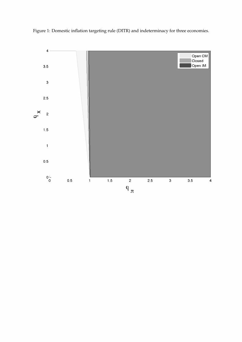
Figure 1: Domestic inflation targeting rule (DITR) and indeterminacy for three economies.

Figure 2: Forecast-based domestic inflation targeting rule (FB-DITR) and indeterminacy forthree economies.

Figure 3: CPI inflation targeting rule (CPITR) and indeterminacy for three economies.

Figure 4: Forecast-based CPI inflation targeting rule (FB-CPITR) and indeterminacy for threeeconomies.

Figure 5: Managed exchange rate targeting rule (MERTR) and indeterminacy for threeeconomies.

Figure 6: Forecast-based managed exchange rate targeting rule (FB-MERTR) and indetermi-nacy for three economies.