1

Thomas R. Berry-Stölzle1

David L. Eckles2

September 2011

* The authors thank Robert E. Hoyt, Jim B. Kau, Henry J. Munneke, and participants of the 2010 Risk Theory Society Seminar for helpful comments and suggestions on this paper. A previous version of this paper was circulated under the title “The Effect of Contracting Incentives on Productivity and Compensation of Insurance Salespersons”. Please address all correspondence to Thomas R. Berry-Stölzle. 1 Terry College of Business, University of Georgia, 206 Brooks Hall, Athens, GA 30602,

Tel.: +1-706-542-5160, Fax: +1-706-542-4295, trbs@terry.uga.edu. 2 Terry College of Business, University of Georgia, 206 Brooks Hall, Athens, GA 30602,

Tel.: +1-706-542-3578, Fax: +1-706-542-4295, deckles@terry.uga.edu.

Incentives of Insurance Salespersons from Future Renewal Commissions*

1

Abstract

We provide an economic explanation for the puzzling observation that there are compensation

schemes with fixed salary components for property-liability insurance salespersons. With an

average policy renewal rate of 89%, selling a policy does not only generate immediate commis-

sion, but also results in (expected) future renewal commissions. This link between current per-

formance and future compensation creates implicit incentives. Our empirical analysis documents

a strong positive relationship between the fraction of renewals and salespersons’ output, and be-

tween renewals and selection of output based compensation schemes. When controlling for

these implicit incentives and self-selection, we do not find a positive effect of output based com-

pensation on sales output.

(JEL G22, J3, J22, J00)

Key Words: Compensation Schemes, Incentives, Career Concerns, Insurance Salespersons

Incentives of Insurance Salespersons from Future Renewal Commissions

2

1. Introduction

Theory in personnel economics builds on the fundamental concept that workers respond to

incentives. Workers who are paid based on their output will ceteris paribus produce more output

than workers receiving a fixed salary. This effect is driven by increased effort levels as well as by

worker sorting; higher ability workers self-select the output based compensation scheme over a

fixed salary to earn a higher compensation (see, e.g., Lazear, 1986, 2000; Brown, 1990, 1992;

Shearer, 2004; Pekkarinen and Riddell, 2008). In dynamic models under asymmetric information,

however, workers have incentives to hide their ability by holding back production in early periods

to avoid more demanding schedules in the future (see, e.g., Freixas, Guesnerie, and Tirole, 1985;

Laffont and Tirole, 1988). This so called ratchet effect makes output based compensation schemes

inefficient (Gibbons, 1987), unless there is a labor market for older workers. Kanemoto and Mac-

Leod (1992) show that competition for older workers permits efficient output based contracts. They

further argue that their result may explain why output based compensation schemes are common in

certain jobs like sales positions, and less popular in other areas like manufacturing.

U.S. property-liability insurance salespersons provide an interesting case. Despite the fact

that there is an active labor market for older and experienced salespersons, there is the full spectrum

of compensation schemes, ranging from fixed salary, combinations of salary and commission, and

compensation entirely based on commission, offered in the industry (see, e.g., Umble, York, and

Leverett, 1977; The National Alliance Research Academy, 2004).

The goal of this paper is threefold. First, we provide an economic explanation for the puz-

zling observation that there are compensation schemes with fixed salary components for property-

liability insurance salespersons. Second, we examine the effect of output based compensation

schemes on worker output using data from U.S. insurance salespersons. Third, we examine factors

determining salespersons’ choice of a compensation scheme.

3

Salespersons receiving a substantial fraction of their compensation as salary do not have

strong direct incentives to deliver high performance. But focusing the discussion on salespersons’

current compensation structure omits an important source of implicit incentives: career concerns –

concerns about the effect of current sales performance on future compensation.1 Most property or

liability insurance contracts are one year contracts, and policyholders usually renew their policy

with the same salesperson.2 Therefore, selling a policy does not only generate immediate commis-

sion, it also results in (expected) future renewal commissions for the insurance agency. Assuming

competition for older experienced salespersons as in Kanemoto and MacLeod (1992), the salesper-

son working for the agency can expect to get a share of her increased production in form of higher

compensation. Thus, salespersons have strong incentives to establish a portfolio of (potential) re-

newal customers, a so-called “book of business.” This mechanism creates indirect sales incentives

regardless of a salesperson’s current compensation scheme and, hence, allows insurance agencies to

offer compensation schemes with a fixed salary component as well as fixed salary contracts.

If a fixed salary salesperson sells a lot and expands her book of business, she will be able to

renegotiate her compensation with the agency owner. Adjustments in compensation are likely to

lag behind changes in production. Therefore, for high ability salespersons it is advantageous to be

on a pure commission compensation scheme that allows them to profit from improvements in pro-

duction immediately.

1 Career concerns were first discussed by Fama (1980); he argued that incentive contracts are not necessary for manag-ers because managers are disciplined by the labor market. If a manager performs well she will get high wage offers, if a manager performs poorly she will get low wage offers. Gibbons and Murphy (1992) study optimal incentive contracts when workers have career concerns. Their results emphasize the importance of optimizing total incentives: the sum of explicit contracting incentives and implicit career concern incentives. Chung, Sensoy, Stern, and Weisbach (2010) examine implicit incentives of private equity general partners from expected future fundraising. They quantify the magnitude of these implicit incentives and conclude that, for general partners of private equity funds, implicit incentives are about as large as explicit incentives. 2 Average policy renewal rates for commercial lines policies sold via independent agencies in the U.S. are 89%; average policy renewal rates for personal lines policies sold via independent agencies are 89% as well (The National Alliance Research Academy, 2006, p. 26).

4

Our analysis is divided into three sections. First, we follow the OLS regression specifica-

tions in the salesperson literature and examine what effect the percentage of commission in the total

compensation package has on sales output and salespersons’ income levels. The broad range of

compensation schemes for insurance salespersons allows a cross-sectional comparison of their im-

pact on sales output. In the context of these regressions, we also examine the relationship between

sales output and the fraction of a salesperson’s production that stems from renewals. Second, to

control for salesperson’s self-selection of compensation schemes, we re-estimate the output and

compensation level models together with a model explaining the choice of a compensation system

with characteristics of the salesperson as well as the job in a simultaneous equation framework.

Third, we employ the Blinder-Oaxaca decomposition (Blinder, 1973; Oaxaca, 1973) and Jann’s

(2008) significance test for the resulting differential, to examine which part of the output difference

between fixed salary and pure commission salespersons can be explained by differences in produc-

tivity characteristics, such as education and work experience. The “explained” part of the output

difference can be attributed to a firm’s ability to hire more productive workers. The unexplained

part of the output difference results from the firm’s salespersons producing more because of incen-

tive effects.

Our empirical analysis provides four main results: First, we find a strong positive relation-

ship between the fraction of renewals and salespersons’ output; and this finding is robust with re-

spect to self-selection of compensation schemes. Second, we find that more established salesper-

sons with a higher percentage of renewals are more likely to choose a pure commission compensa-

tion scheme. Third, when controlling for self-selection of compensation schemes, we do not find a

positive effect of output based compensation on sales output. Fourth, salespersons’ compensation is

mainly determined by their sales output. Overall, these findings support the view that insurance

5

salespersons have strong incentives to build a book of business, and that these indirect sales incen-

tives allow insurance agencies to offer compensation schemes with a fixed salary component.

Our research contributes to numerous strands of the literature. First, we provide new empir-

ical evidence to the idea pioneered by Fama (1980) that career concerns can be an important source

of incentives inside firms. Second, we contribute to the insurance literature by studying the perfor-

mance impact of compensation schemes for insurance salespersons for the first time.3 Third, we

extend the marketing literature by using a simultaneous equation model to address the endogeneity

of compensation scheme choice in analyzing the relationship between compensation schemes and

sales performance.

The remainder of this article is organized as follows. The next section introduces the institu-

tional environment we examine, i.e. independent insurance agencies. The third section provides the

conceptual background and explains the development of the hypotheses. The data and methodology

are discussed in the fourth section of the article including a detailed description of the measures

used in the empirical analysis. The fifth section presents the empirical results, and the final section

concludes.

2. Independent Insurance Agencies

In the U.S., insurance products are sold via two main distribution channels.4 Some insurers,

referred to as direct writers, employ their own sales force to primarily (if not exclusively) sell their

products. Other insurers utilize independent agencies to distribute their insurance products. Unlike

direct writers, independent agencies typically represent multiple insurers. Another important cha-

3 The existing literature on insurance sales focuses on the choice of a distribution channel from the point of view of the insurance company (see, e.g., Won-Joong, Mayers, and Smith, 1996). Since all types of distribution systems have their specific advantages and disadvantages, the fit between the distribution system and insurer and market characteristics is important (Zweifel and Ghermi, 1990; Barrese, Doerpinghaus, and Nelson, 1995; Berger, Cummins, and Weiss, 1997; Regan, 1997; Regan and Tzeng, 1999; Brockett, Cooper, Golden, Rousseau, and Yuying, 2005; Trigo-Gamarra, 2008). 4 For a more detailed discussion of insurers’ distribution channels in the U.S. see, e.g., Regan and Tennyson (1996, 2000).

6

racteristic of independent agencies is that they own their book of business. This means that an in-

surance company is not allowed to contact policyholders directly to renew their policies or to sell

them additional products; all communication between the insurer and the policyholder has to go

through the agency.

While some of the independent agencies consist of only one self-employed agent, most

agencies are corporations with multiple employees. Employees whose primary task it is to sell in-

surance are called producers. Producers of this type make up approximately 51% of insurance sales

agents (Bureau of Labor Statistics, 2009). Whenever a producer sells an insurance policy of one of

the insurers represented by the agency, the agency receives commission from the corresponding

insurance company. Sales commissions are the most important source of revenues for independent

agencies as they account for 87% of agency revenues (The National Alliance Research Academy,

2006). Therefore, the amount of sales commission generated by a producer directly measures the

producer’s sales production, and this production measure is directly observable by the agency own-

ers.

However, the fact that insurance companies compensate independent agencies on a commis-

sion basis does not imply that independent agencies compensate all their producers on a pure com-

mission basis. In fact, agencies offer the full spectrum of commission based compensation

schemes, ranging from a fixed salary (no commissions) to compensation entirely based on commis-

sion (one hundred percent commissions). Umble, York, and Leverett (1977) surveyed independent

insurance agencies in the state of Georgia regarding producers hired in a three year window. They

report that 54% of the 239 newly hired producers in their sample were paid only a salary, 29% re-

ceived a combination of salary and commission, and 17% were paid on a commission only basis.

More recently, the National Alliance Research Academy (2004) surveyed producers working in

independent agencies across the United States. They distinguish between producers mainly selling

7

commercial property-liability insurance products and producers mainly focusing on personal lines.

They report that 12% of the commercial lines producers in their sample are paid a salary only,

49% are paid with a mixed compensation scheme, and 39% are paid commission only.5 We use this

variation in compensation structures across producers working for independent insurance agencies

to analyze the impact of different compensation structures on the producers’ sales output.

Note that we only focus on property-liability insurance sales in our discussion because con-

tractual incentives in life insurance sales are substantially different from contractual incentives in

property-liability insurance sales.6 However, this is not very restrictive since life and health insur-

ance commissions account for only about 10% of revenue of independent agencies (The National

Alliance Research Academy, 2006).

Most property or liability insurance contracts are one year contracts. On average, 89% of

policyholders renew their existing policy at the end of the contract term.7 Thus, selling a policy

does not only generate immediate commission for the agency, it also results in (expected) future

renewal commissions. Insurance companies usually pay independent agencies the same percentage

commission for renewals as for new business (Regan and Tennyson, 2000); otherwise, independent

agencies would have strong incentives to switch their clients to another insurance company after the

first policy term. Producers working for an agency, however, usually receive a slightly lower re-

newal commission rate than new business commission rate from their agency. Standard commis-

sion rates for a commercial lines producer on a pure commission compensation scheme are 40% for

5 In the same sample, compensation for personal lines producers slightly differs with 19% paid a salary only, 54% paid with a mixed pay scheme, and 27% paid commission only. 6 In contrast to property-liability insurance salespersons, the vast majority of life insurance salespersons work on a pure commission compensation scheme. Commission schemes usually pay large first year commissions for new business, but hardly any commissions in later years of a policy, or for renewals (Regan and Tennyson, 2000). The turnover rate for life insurance agents is 26% per year, and the average four year retention rate for new agents is only 18% (Hoesly, 1996). 7 Average policy renewal rates for commercial lines policies sold via independent agencies in the U.S. are 89%; average policy renewal rates for personal lines policies sold via independent agencies are 89% as well (The National Alliance Research Academy, 2006, p. 26).

8

new business and 35% for renewals.8 This means that the producer receives 40% (35%) of the

commission which the agency receives from the insurance company for each policy sold (renewed).

Commission rates are lower if a producer’s compensation package also includes a fixed salary com-

ponent.9

Table 1 provides an example highlighting the importance of expected renewal commissions

for commercial lines producers. Assuming that the producer sells a policy that generates $2,500 in

commission for the agency, and assuming a 40% commission rate, the producer earns $1,000 on

this sale.10 Panel B of Table 1 calculates the present value of expected renewal commissions the

producer will receive from this sold policy. The ten year evaluation framework, the two percent

inflation rate and the ten percent discount rate we use are based on Trieschmann, Davis, and Leve-

rett’s (1975) valuation model for property-liability insurance agencies. The calculation assumes an

89% renewal rate and a renewal commission rate of 35%. Column 7 presents the ratio of the

present value of expected renewal commissions to the first year commission the producer receives.

If the producer stays in business for 10 years, the present value of expected renewal commissions is

3.5-times as big as the first-year commission on the policy sold. If the producer quits after 2 years,

the present value of expected renewal commissions is still larger than the first-year commission as

the ratio is 1.32. Since retention rates of producers are relatively high in independent agencies, ex-

pected renewal commissions play an important role for these salespersons.11

8 The median share of new business commission that a commission-only producer in our sample can keep is 40%; the median share of renewal commission that a commission-only producer in our sample can keep is 35%. The data is described in Section 4. 9 The median share of new business commission that a mixed pay producer in our sample can keep is 33%; the median share of renewal commission that a mixed pay producer in our sample can keep is 30%. The data is described in Sec-tion 4. 10 The median commission per policy agencies in our sample receive is $2,500. The data is described in Section 4. 11 Umble, York, and Leverett (1977) surveyed independent insurance agencies to calculate the retention rate of produc-ers. They report that 85% of producers hired two to five years prior to the survey were still with the agency. This 85% retention rate for property-liability producers contrasts with the 18% average four year retention rate for new life insur-ance agents reported by Hoesly (1996).

9

In the remainder of the paper we will use the terms producer and insurance salesperson in-

terchangeably to refer to such salespersons working for independent insurance agencies.

3. Conceptual Background and Hypotheses Development

Theory predicts that profit maximizing firms select compensation schemes for their work-

force by comparing the respective costs and benefits of these schemes (Hart and Holmström, 1987;

Journal of Labor Economics, 1987). Benefits of an output based compensation scheme in static

models under asymmetric information include incentives to exert more effort (Holmström, 1979)

and the attraction of higher ability workers (see, e.g., Lazear, 1986, 2000; Brown, 1990, 1992;

Shearer, 2004; Pekkarinen and Riddell, 2008). When workers of different abilities are faced with a

choice between an output based compensation scheme and a fixed salary, higher ability workers

prefer and, hence, select an output based compensation scheme that allows them to earn more than

the fixed salary.

In dynamic models under asymmetric information, however, output based compensation

schemes may be inefficient. A worker’s performance provides information about the worker’s un-

observable ability. In a long-term employment relationship, a firm can use the information revealed

by observing the worker’s output to set performance standards in the future. Anticipating this be-

havior, a worker has incentives to hide her ability by holding back production in early periods to

avoid more demanding schedules in the future (see, e.g., Freixas, Guesnerie, and Tirole, 1985; Laf-

font and Tirole, 1988). This is referred to as the ratchet effect. Two important characteristics of

models explaining the ratchet effect are that firms cannot commit to long-term contracts and that

workers have only limited (if any) employment alternatives in later periods (see, e.g., Gibbons,

1987). Kanemoto and MacLeod (1992) show that competition for older workers permits efficient

output based contracts. Their model includes a job market for older workers with output based

10

compensation contracts. This model implies that workers’ employment alternatives in later periods

depend on the ability of the workers. Kanemoto and MacLeod’s result holds even if workers make

some relationship-specific investments that create positive mobility costs. Since there is an active

job market for older and experienced property-liability insurance producers in the U.S., we expect a

pure commission contract between an agency and a producer to be an efficient compensation

scheme.

Pure commission compensation schemes provide direct sales incentives for producers.

However, in his analysis of managers, Fama (1980) argues that incentive contracts are not neces-

sary because workers are disciplined by the labor market. If a worker performs well she will get

high wage offers, if she performs poorly she will get low wage offers. Therefore, concerns about

the effect of current performance on future compensation create an important source of implicit

incentives for workers. Formal models of such career concerns are usually based on a learning

framework (see, e.g., Gibbons and Murphy, 1992; Chung, Sensoy, Stern, and Weisbach, 2010); the

labor market uses a worker’s current performance to update its beliefs about the worker’s ability

and then bases future wages on these updated beliefs. In the case of property-liability insurance

salespersons, one can argue that the current size of their book of business as well as the fraction of

their sales generated by renewal business are observable signals of their ability. Thus, a learning

model can be used to explain the existence of career concerns incentives of insurance salespersons.

A producer’s employability in the external labor market changes as agencies update their beliefs

about the producers ability. With respect to the internal labor market within the producer’s current

agency, however, expected future renewal commissions create a direct link between current and

future performance. Since about 89% of policyholders renew their existing policy at the end of the

contract term, selling a policy does not only generate immediate commission, it also results in (ex-

pected) future renewal commissions for the insurance agency. Assuming competition for older ex-

11

perienced salespersons as in Kanemoto and MacLeod (1992), the salesperson working for the agen-

cy can expect to get a share of her increased production in form of higher compensation. Thus, sa-

lespersons have strong incentives to establish a portfolio of (potential) renewal customers, a so-

called book of business. This mechanism creates indirect sales incentives regardless of a salesper-

son’s current compensation scheme. Using the fraction of a salesperson’s sales production from

renewals as a measure of ability for building a book of business, we can formulate the following

two testable hypotheses: (H1) Salespersons with a higher fraction of sales production from renewals

are, on average, more productive than salespersons with a lower fraction of production from renew-

als, and (H2) more productive salespersons earn, on average, a higher compensation than less pro-

ductive salespersons.

In a learning model where the labor market uses a worker’s current performance to update

its beliefs about the worker’s ability, information in earlier time periods is more valuable to the

market than information in later periods (Chung, Sensoy, Stern, and Weisbach, 2010). Thus, the

sensitivity of future compensation to the fraction of sales production from renewals should decrease

in the producer’s years of experience.

Furthermore, there is a limit on how many accounts a producer can handle. If a producer al-

ready has a large book of business then the producer is busy taking care of all renewals and has lit-

tle time left to sell policies to new clients. Assuming that first, all producers are working towards

building a book of business and that second, it takes a number of years to establish a book of busi-

ness, we can formulate the following testable implication: (H3) The sensitivity of future sales per-

formance to the fraction of sales production from renewals should decrease in the producer’s years

of experience.

Overall, the existence of implicit sales incentives from expected future renewal commission

allows insurance agencies to offer compensation schemes with a salary component as well as fixed

12

salary contracts. As Gibbons and Murphy (1992) point out, optimal incentive contracts in the pres-

ence of career concerns should be based on total incentives: the sum of explicit incentives from the

compensation contracts and implicit incentives from career concerns. Since career concern incen-

tives are especially pronounced at earlier career stages, a fixed salary may be the optimal compensa-

tion structure for relatively new salespersons. Gibbons and Murphy (1992) argue that explicit in-

centives from the compensation scheme should be strongest for older workers reaching retirement

because career concerns are less important for those workers. However, the case of older expe-

rienced property-liability insurance salespersons with an established book of business is slightly

different. Because of the established book of business, the largest fraction of the salesperson’s total

sales production will come from renewals which are predictable. Even if the salesperson reduces

her sales effort completely, existing customers will still renew with a probability of 89%.12 Thus,

there is a lower bound on the salesperson’s production that allows agencies to offer a fixed salary

contract. However, whether salespersons prefer a fixed salary or a pure commission compensation

scheme is another issue.

In Kanemoto and MacLeod’s (1992) model with competition for older experienced salesper-

sons, a salesperson who sells a lot and expands her book of business can expect to get a share of her

increased production in form of higher compensation. If the salesperson is on a pure commission

compensation scheme, compensation directly increases with sales. However, if the salesperson is

on fixed salary she will have to renegotiate her compensation with the agency owner, and because

of this negotiation process, adjustments in compensation are likely to lag behind changes in produc-

tion. Thus, for high ability salespersons it is advantageous to be on a pure commission compensa-

tion scheme that allows them to profit from improvements in production immediately. Using the

fraction of a salesperson’s sales production from renewals as a measure of ability for building and 12 Average policy renewal rates for commercial lines policies sold via independent agencies in the U.S. are 89%; aver-age policy renewal rates for personal lines policies sold via independent agencies are 89% as well (The National Al-liance Research Academy, 2006, p. 26).

13

maintaining a book of business, we can postulate the following hypothesis: (H4) Salespersons with

a higher fraction of sales production from renewals are, on average, more likely to choose a pure

commission compensation scheme than salespersons with a lower fraction of production from re-

newals.

4. Data and Methodology

4.1 Data

Our data comes from the third survey of producer compensation, collected by the National Al-

liance Research Academy in 2003. We use the commercial lines producer portion of their original

dataset.13 Producers are classified as commercial lines producers if they derive 60% or more of

their total sales volume from commercial lines business. The data provides descriptive information

on sales production, producer compensation, as well as producer and agency characteristics. There

are 307 commercial lines producers in the dataset and approximately two-thirds answered all of the

survey questions required for our study. Therefore, we are left with 196 producers in our sample.14

Forty-three percent of these producers are paid only by commissions, while 14% of the producers

are paid only a fixed salary. The remaining 43% are compensated with both salary and commis-

sions. Ultimately, 63% of the average producer’s income comes from commissions.15

13 We would like to thank the National Alliance Research Academy for providing us access to an anonymous version of the original survey responses of the commercial lines producers. A descriptive analysis of the survey was published by the National Alliance Research Academy in 2004 under the title “Producer Profile: Compensation, Production, and Responsibilities.” 14 The distribution of compensation schemes among the 197 producers with usable data is similar to the distribution of compensation schemes among all 307 commercial lines respondents. 15 There is very little information available for the population of insurance salespersons in the U.S. Thus, it is difficult to test for sample selection bias. A 2006 report by Research and Markets (http://www.researchandmarkets.com) pro-vides a few basic descriptive statistics of the U.S. insurance agency market. Comparing these statistics to our sample indicates that our sample is rather representative of the U.S. insurance agency market. Research and Markets reports that the average agency consists of 5 employees. Though the average size of our sample is larger (19.2), the median size in our sample is 6 employees. Additionally, the report by Research and Markets shows the average revenue per em-ployee to be approximately $200,000. Again, the average revenue for the employees in our sample is slightly higher ($299,963), though the median is very near the average reported by Research and Markets ($205,000).

14

4.2 Methodology

We analyze the effects of explicit incentives from output based compensation schemes and

implicit incentives from expected future renewal commissions on salespersons’ production in four

steps. First, we regress sales output on the percentage of commission in the total compensation

package and on the percentage of renewals. Second, we regress salespersons’ income levels on

sales output as well as the percentage of commission in the total compensation package. Third, to

control for salespersons’ self-selection of compensation schemes, we re-estimate the output and

compensation regression models together with a model explaining the choice of a compensation

system in a simultaneous equation framework. Fourth, we employ the Blinder-Oaxaca decomposi-

tion to decompose the output difference between fixed salary and pure commission salespersons

into a component explained by salespersons’ characteristics and an unexplained component.

4.2.1 Productivity Regression Models

Our analysis of the impact of output based compensation schemes and renewals on salesper-

sons’ production is based on an ordinary least squares (OLS) regression model. The specification of

the model is as follows:

1 2 3% %i i i i iLogProduction Commission Renewals Xα β β β ε′= + + + + (1)

where LogProductioni is the natural logarithm of the commissions paid by insurance companies to

the agency for sales generated by producer i in one year, %Commissioni is the fraction of output-

based compensation or commission producer i receives from the agency as a percent of the produc-

er’s total compensation, %Renewalsi is the fraction of producer i‘s sales production from renewals

15

as a percent of the producer’s total sales production, X is a vector of control variables, and ε is a

random error term.16

To control for differences in the producers’ marginal productivity of sales effort (see, e.g.,

Basu, Lal, Srinivasan, and Staelin, 1985), we include YearsWithAgency and InsuranceExperience

variables in the regression model. YearsWithAgency measures the number of years the producer has

worked for the current agency. We expect YearsWithAgency to be positively related to sales pro-

ductivity. The InsuranceExperience variable measures the years of experience in insurance sales.

In addition, we use a number of variables to control for agency specific characteristics. In

some agencies, producers have to take on administrative duties as well. Therefore, we include

%TimeSelling as a variable in the model; this variable measures the percent of the producer’s work

week allocated towards selling. Alternatively, producers might also receive sales support from the

agency. To control for differences in sales support, the model includes Support as a variable which

captures the number of full-time-equivalent support staff assisting the producer. The size of the

agency can also influence sales output due to economies of scale and name recognition. Therefore,

we include AgencySize as a variable in the model; this variable measures the number of full-time

producers employed by an agency. To control for a possible difference between rural and urban

areas, we include LargeCity as a variable in the model. This dummy variable is coded as 1 if the

agency is located in a city with more than 2,000,000 inhabitants and 0 otherwise.

To examine whether the sensitivity of sales performance on the fraction of sales production

from renewals decreases in the producer’s years of experience, we estimate the following extension

of Equation (1):

16 The %Renewals variable should not create an endogeneity problem for the following two reasons: First, by construc-tion, the fraction of renewals is (mainly) determined by a salesperson’s past (or lagged) sales production. Second and most importantly, the %Renewals variable is not significantly correlated with the error term in any of the regression models. We examine the correlation coefficients and find that they are close to zero and not significant at the 10-percent significance level. As Baum (2006) points out, from a statistical perspective, a variable in a regression model is endo-genous and may cause inconsistent estimates if the variable is correlated with the disturbance term. It is this “definition of endogeneity that matters for empirical work” (Baum, 2006, p. 185).

16

1 2

3 4

% %%

i i i

i i i i

LogProduction Commission RenewalsRenewals YearsWithAgency X

α β ββ β ε

= + +′+ × + +

(2)

with the additional interaction term % i iRenewals YearsWithAgency× , and all other variables as spe-

cified in Equation (1). A negative and significant estimate for 3β provides support for Hypothesis

H3.

4.2.2 Compensation Regression Model

To establish the existence of career concern incentives for salespersons, we not only need to

show that the fraction of renewals has a positive impact on sales production, but we also need to

show that sales production has a positive impact on producers’ compensation. Thus, we estimate

the following OLS regression model:

1 2i i i iLogTotalCompensation LogProduction Xα β β ε′= + + + (3)

where LogTotalCompensationi is the natural logarithm of the producer’s total annual compensation,

LogProductioni is the natural logarithm of the commissions paid by insurance companies to the

agency for sales generated by producer i in one year, X is a vector of control variables, and ε is a

random error term.

The set of control variables includes %Commission as a variable to control for the impact of

output-based compensation schemes on producer compensation (Parent, 1999, 2009; Aggarwal and

Samwick, 2006). Since producers’ opportunity cost of time depends on the value of their human

capital, we include YearsWithAgency, InsuranceExperience and BachelorsDegree variables in the

model to control for differences in human capital investments (Coughlan and Narasimhan, 1992).

BachelorsDegree is a dummy variable equal to one if the highest level of education attained is a

bachelor’s degree. To capture differences in additional compensation-like benefits, we include

Pension and TravelExpenses variables; these two variables are dummy variables equal to one if the

17

agency provides pension benefits, and if the agency provides reimbursement for travel expenses,

respectively. To control for differences in agency location, we again include the LargeCity varia-

ble. We also include FirstJob as a dummy variable which is equal to one if the current position is

the producer’s first job, and zero otherwise. We expect this variable to be negatively related to the

producer’s total compensation because of the lack of negotiating power when looking for an entry

level position.

To ensure that our results are not distorted by producers self-selection of a compensation

scheme, we also estimate a simultaneous equation model consisting of Equations (1) and (3) and a

third equation explaining the choice of a compensation system.

4.2.3 Simultaneous Equation Model

Our analysis of factors determining the choice of a compensation system is based on the

model specified in Equation (4). We estimate Equation (4) together with Equations (1) and (3) with

three-stage least squares (3SLS). This approach allows us to check whether the results from the

productivity and earnings regressions are distorted by potential endogeneity resulting from the fact

that the choice of a compensation system is usually not random. The choice of the compensation

scheme is modeled as follows:

1 2% i i i iCommission Ability Xα β β ε′ ′= + + + (4)

where % iCommission is the fraction of output-based compensation producer i receives as a percent

of total compensation, Ability is a vector of variables measuring producers’ ability, X is a vector of

control variables, and ε is a random error term.

Variables measuring a producer’s ability to sell include the fraction of a producer‘s sales

production from renewals, %Renewals, the number of years the producer works for the current

18

agency YearsWithAgency, the years of experience in insurance sales InsuranceExperience as well as

the BachelorsDegree dummy variable.

Since administrative support staff in an agency usually receives a fixed salary, we expect

producers who take on administrative duties to get a substantial fraction of their compensation as

fixed salary as well. On the other hand, producers who allocate their complete work week towards

selling may be more likely to be on an output based compensation scheme. Thus, we include

%TimeSelling as control variable in the model.

Travel expenses borne by the agency shift risk from the individual producer to the agency.

Every sales call is risky because there is a change that this call may be non-productive. An agency

bearing the producer’s expenses increases the certainty equivalent value of the producer’s compen-

sation package. Coughlan and Narasimhan (1992) argue that agencies bearing producers’ expenses

can, hence, offer compensation packages with a larger fraction of “risky” output-based compensa-

tion. On the other hand, one cannot expect employees receiving a fixed salary to pay for travel ex-

penses. Therefore, an alternative hypothesis is that agencies bearing producers’ expenses should be

more likely to offer fixed salary compensation. To control for any effect of expense reimbursement

schemes on compensation packages, we include TravelExpenses as a variable in the model.

If a producer does not find a suitable fit in her current agency, the producer might start look-

ing for a new job that better suits her ability. When selecting a new job, one of the criteria that

plays a role in the producer’s decision is the job’s compensation structure. To capture differences in

producers’ selection of compensation schemes when leaving their previous agency because of a lack

of fit, we include OtherGoals as a variable in the model. OtherGoals is a dummy variable coded as

one if the producer left the previous job because the previous agency did not meet the producer’s

19

expectations or because she did not meet the previous agency’s expectations.17 Since high ability

salespersons should be able to be successful in various environments, “fit” is likely to be more of an

issue for lower ability salespersons. Thus, we expect OtherGoals to be negatively related to the

fraction of output-based compensation in the total compensation package.

4.2.4 Blinder-Oaxaca Decomposition

To further examine differences in sales output between the two groups of fixed salary and

pure commission salespersons, we employ the Blinder-Oaxaca decomposition method (Blinder,

1973; Oaxaca, 1973). For two groups of observations, an outcome variable and a set of predictor

variables, the Blinder-Oaxaca decomposition gives an answer to the question how much of the dif-

ference in the two group means of the outcome variable can be explained by group differences in

the predictors? Originally, this method was used by Blinder (1973) and Oaxaca (1973) to study

wage discrimination between male and female workers. The part of the wage differential that could

not be explained by group differences in productivity characteristics was interpreted as a measure of

discrimination. In our analysis, we focus on what fraction of the output difference between fixed

salary and pure commission salespersons can be explained by differences in productivity characte-

ristics, such as work experience. To correct for salespersons’ self-selection of compensation

schemes, we deduct the selection effects from the overall output difference first, and then examine

the corrected output difference (Reimers, 1983). The part of the corrected output difference that

cannot be explained by different “endowments” of fixed salary and pure commission salespersons

can be interpreted as a pure incentive effect: A pure commission environment ceteris paribus in-

17 The variable OtherGoals is generated from survey questions asked regarding the rationale for a producer leaving her last job. Respondents are asked why they left their previous job and are given eight choices in addition to an “other” option. If the producer responded with “Inadequate dollar compensation,” “Inadequate benefits,” “Poorly managed agency,” “Inadequate support staff,” “Low Personal Production” or “Long Work Hours,” OtherGoals is set to one. It should be noted that if the producer is in her first job, OtherGoals is zero. Therefore, OtherGoals should be interpreted as the effect that experienced producers’ goals have on their total compensation.

20

duces producers to exert more effort and, hence, increases output. Thus, the Blinder-Oaxaca de-

composition allows us to test whether there is an incentive effect in addition to a sorting effect, i.e.

more productive workers self-select into positions offering a pure commission compensation

scheme.

We perform the decomposition for the two groups of commission-only and salary-only pro-

ducers and for the outcome variable LogProduction. More precisely, we estimate Equation (1)

without the %Commission variable separately for the two groups of commission-only and salary-

only producers, including a correction term for self-selection.18 We derive the self-selection correc-

tion term based on a probit estimation of Equation (4) using a CommissionOnlyDummy as the de-

pendent variable (Maddala, 1983, pp. 120-121).19 As suggested by Reimers (1983), we then take

the output difference after deducting the selection effects and apply the standard decomposition

formulas. We use the twofold decomposition procedure with coefficients from a pooled regression

over both groups as the reference case as outlined in Neumark (1988) and Jann (2008) and correct

standard errors for sampling variances.20,21

18 Let the index c denote the group of commission-only producers and the index s denote the group of salary-only pro-ducers. Since ( ) 0E ε = , the mean outcome difference between the two groups is

ˆ ˆ ˆ ˆ( ) ( ) ( ) ( ) ( ) ( )c s c c s s c c s sE LogProduction E LogProduction E X E X E h E hβ β δ δ′ ′− = − + −

where ˆ ˆ( ) ( )c c s sE h E hδ δ− corrects for self-selection effects, and the hazard ih is calculated as described in Footnote 15. 19 In a first step, probit estimates are obtained of the equation Pr( 1 | ) ( )i i iCommissionOnlyDummy X Xγ ′= = Φ , where X is the vector of independent variables from Equation (4), and Φ is the cumulative distribution function of the standard normal distribution. From these estimates, the correction term or hazard, hi, for each observation i is then calculated as:

ˆ ˆ( ) / ( ), 1

ˆ ˆ( ) / (1 ( )), 0i i i

i

i i i

X X if CommissionOnlyDummyh

X X if CommissionOnlyDummy

φ γ γ

φ γ γ

′ ′Φ ==

′ ′− − Φ =

⎧⎨⎩

where φ is the standard normal density function. 20 The twofold decomposition procedure assumes that there is a nondiscriminatory coefficient vector that should be used as a basis for determining the contribution of the differences in the predictors. We can use the coefficients *β̂ from a pooled regression over both groups as such a nondiscriminatory coefficient vector. The outcome difference between the two groups can then be written as: * * *ˆ ˆ ˆ ˆ ˆ( ) ( ) ( ) ( )) { ( )( ) ( )( ) }(c s c s c sc sE LogProduction E LogProduction E X E X E X E Xβ β β β β′ ′ ′− = − + +− −

21

5. Results

Table 2 contains summary statistics for our dataset. The producers in our sample generate an

average of almost $300,000 in revenue for the agency and on average earn approximately $119,000

in annual income. The agencies in the sample vary quite a bit in size. The smallest agency has only

1 producer while the largest agency has 500 producers; the median is 6 producers per agency. Ap-

proximately 20% of the agencies are in “large cities” with more than 2,000,000 inhabitants, and the

remaining 80% of the agencies are in more rural areas. With respect to the producers themselves,

approximately half of the respondents are in their first job as a producer, and the average producer

has approximately 14 years of experience in the industry.

Graph 1 of Figure 1 presents kernel density estimates of the LogProduction variable for the

three compensation schemes salary-only, mixed pay and commission-only, separately. For salary-

only producers, the peak of the estimated density function as well as the center of the distribution

are further left than for the group of producers receiving mixed pay, and the peak and center of the

distribution for mixed pay producers is further left than for commission-only producers. These

findings provide some preliminary evidence of a positive association between output-based com-

pensation schemes and production levels.

Graph 2 of Figure 1 presents kernel density estimates of the LogTotalCompensation variable

for the three compensation schemes salary-only, mixed pay and commission-only, separately. Simi-

lar to the findings for the LogProduction variable, we observe that the peak and the center of the

estimated density function for salary-only producers are to the left of the function’s peak and center

for mixed pay producers, and the peak and the center of the density function for mixed pay produc- where *ˆ ( ) ( ))( c sE X E Xβ ′ − is the part of the outcome difference that is explained by differences in the predictor varia-

ble (“endowment” effect), and * *ˆ ˆ ˆ ˆ{ ( )( ) ( )( ) }c sc sE X E Xβ β β β′ ′+− − is the unexplained part of the outcome differen-tial. 21 Following Jann’s (2008, p. 458) suggestion, we also include a group dummy in the pooled regression model as an additional covariate. The group dummy variable is coded as 1 if the producer belongs to the salary-only group, and 0 otherwise.

22

ers are to the left of the function’s peak and center for commission-only producers. These findings

indicate a positive association between output-based compensation schemes and earnings. In addi-

tion, the distributions of the LogTotalCompensation variable look similar to the distributions of the

LogProduction variable indicating a positive relationship between sales production and salesper-

sons’ compensation.

Table 3 contains summary statistics for the three groups of salary-only producers, mixed pay

producers, and commission-only producers, separately. We can see that salary-only producers have

on average more experience (17 years vs. 15 years), a less established client base (%Renewals =

63% vs. 75%), and that a higher fraction of salary-only producers gets sales reimbursement for tra-

vel expenses (89% vs. 54%).

5.1 Productivity Regression Models

5.1.1 OLS Results

The OLS estimation results from Equation (1) are presented in column 1 of Table 4. The re-

gression coefficient of the %Commission variable is positive and significant, indicating a positive

relationship between the fraction of output-based compensation in the compensation package and a

producer’s sales production. Most importantly, the regression coefficient of the %Renewals varia-

ble is positive and significant. This result supports Hypothesis H1 which states that salespersons

with a higher fraction of sales production from renewals are more productive than salespersons with

a less established book of business.

In addition, two of the control variables have a significant impact on LogProduction. The

coefficient of the Support variable is positive, indicating that the availability of support staff in-

creases a producer’s sales production. The coefficient of the LargeCity variable is also positive,

indicating that average sales production is higher in large cities with over two million inhabitants.

23

As a robustness check, Column 2 of Table 3 presents the OLS estimation results from an al-

ternative specification of Equation (1); the %Commission variable is replaced by the Commissio-

nOnlyDummy variable which is coded as 1 of the producer is on a commission only compensation

scheme, and 0 otherwise. The results of this alternative specification are consistent with the ones

from the baseline model.

Columns 3, 4 and 5 of Table 4 show the OLS estimation results from Equations (1) for the

subsamples of commission-only producers, mixed-pay producers and salary-only producers, respec-

tively. For all three subsamples, the regression coefficient of the %Renewals variable is positive

and significant, indicating that an established client base is positively associated with sales produc-

tion for all three types of compensation schemes. These results provide additional support for Hy-

pothesis H1.

Column 1 in Panel A of Table 5 presents the OLS estimation results from Equation (2). The

regression coefficient of the %Commission variable is positive and significant, indicating a positive

relationship between the fraction of output-based compensation in the compensation package and a

producer’s total compensation. The regression coefficient of the %Renewals variable is positive

and significant, and the coefficient of the % i iRenewals YearsWithAgency× interaction term is nega-

tive and significant. These findings indicate that establishing a book of business of (potential) re-

newal customers increases sales production, but at a decreasing rate. Thus, these results support

Hypothesis H3.

To check the robustness of our results with respect to Hypothesis H3, we estimate a number

of additional models. Column 2 in Panel A of Table 5 presents the OLS results from an alternative

specification of Equation (2); the %Commission variable is replaced by the CommissionOnlyDum-

my variable. The results in Column 2 are consistent with the ones from the original model pre-

sented in Column 1. Columns 3, 4 and 5 in Panel A of Table 5 show the OLS estimation results

24

from Equations (2) for the subsamples of commission-only producers, mixed-pay producers and

salary-only producers. For the groups of commission only producers and mixed pay producers, the

positive effect of establishing a book of business on sales production decreases in the producer’s

years with the agency; the % i iRenewals YearsWithAgency× interaction term is negative and signifi-

cant. However, for the subsample of salary only producers, we do not find this relationship.

While the analysis presented in Panel A of Table 5 focuses on the interaction effect between

the %Renewals variable and the YearsWithAgency variable, the analysis presented in Panel B ex-

amines the interaction effect between %Renewals and InsuranceExperience. The InsuranceExpe-

rience variable captures a producer’s total years of experience in insurance sales. The results pre-

sented in Columns 1 and 2 are based on OLS estimates of the complete sample; the only difference

between the two models is that one includes the %Commission variable and the other includes the

CommissionOnlyDummy. In both models, the regression coefficient of the %Renewals variable is

positive and significant, and the coefficient of the % i iRenewals InsuranceExperience× interaction

term is negative and significant. Consistent with Hypothesis H3, these findings support the view

that the positive effect of establishing a book of business on sales production decreases in the pro-

ducer’s years of experience. Columns 3, 4 and 5 present OLS estimates for the subsamples of

commission-only producers, mixed-pay producers and salary-only producers, respectively. For all

three subsamples, the coefficient of the %Renewals variable is positive and significant, and for the

group of salary only producers, the coefficient of the % i iRenewals InsuranceExperience× interac-

tion term is negative and significant.

Overall, our empirical results for Equations (1) and (2) provide support for Hypotheses H1

and H3 which state that there is a positive link between the fraction of sales production from renew-

als and sales production, but that the sensitivity of sales production to renewals decreases in the

producer’s years of experience.

25

5.1.2 Productivity Regression Results Controlling for Self-Selection of Compensation Structure

Columns 1, 2 and 3 of Table 7 show the 3SLS estimation results from Equations (1) and (2).

The simultaneous equation model addresses potential endogeneity with an additional equation ex-

plaining a salesperson’s self-selection of a compensation system with characteristics of the salesper-

son as well as the job. In all three models, the regression coefficient of the %Renewals variable is

positive and significant, and the coefficients of the % i iRenewals YearsWithAgency× and the

% i iRenewals InsuranceExperience× interaction terms are negative and significant in models 2 and

3, respectively. Therefore, we find further support for Hypotheses H1 and H3, indicating a positive

relationship between the fraction of renewals and sales production, but at a decreasing rate.

Interestingly, the regression coefficient of the %Commission variable is not significant in the

three models controlling for salespersons’ self-selection of compensation schemes. This result indi-

cates that the positive effect of output-based compensation on a producer’s sales production found

in OLS estimations is only driven by a self-selection effect.

Columns 7, 8 and 9 of Table 7 show the results of an alternative treatment effects estimation.

The models include the endogenous CommissionOnlyDummy instead of the %Commission variable.

The model is estimated with the two-stage approach described in Maddala (1983, pp. 117-122).

The results are consistent with the ones obtained from the baseline model: We find support for Hy-

potheses H1 and H3; however, we do not find a significant relationship between output-based com-

pensation on sales production when controlling for self-selection of compensation schemes.

5.2 Compensation Regression Model

5.2.1 OLS Results

To test Hypothesis H2 that more productive salespersons earn a higher compensation than

less productive salesperson, we regress salespersons’ LogTotalCompensation on their LogProduc-

26

tion and controls (see Equation (3)). The OLS estimation results are presented in Panel A of Table

6. Column 1 shows the results for the baseline model as specified in Equation (3), Column 2

presents the results for the alternative specification with the CommissionOnlyDummy instead of the

%Commission variable, and Columns 3, 4 and 5 show the regression results for the subsets of

commission-only producers, mixed-pay producers and salary-only producers. In all five models,

the regression coefficient of the LogProduction variable is positive and significant. These findings

provide support for Hypothesis H2.

Panel B of Table 6 presents results for OLS regressions of LogTotalCompensation on Log-

Production and without (most) control variables. The only additional variable included captures

differences in compensation schemes. Again, the regression coefficient of the LogProduction vari-

able is positive and significant in all five models. When comparing the R2 statistics of the regres-

sions in Panels A and B of Table 6, we see that most of the variation in the dependent variable Log-

TotalCompensation is explained by producers’ LogProduction alone, the additional variables in-

cluded in Panel A only slightly improve the model fit.

Overall, these results combined with the results presented in the previous section provide

empirical support for the existence of career concern incentives for insurance salespersons. Build-

ing a book of business consisting of (potential) renewal customers positively impacts future sales

performance, and sales performance directly impacts salespersons’ compensation. This link be-

tween current performance and future compensation creates strong incentives to sell.

5.2.2 3SLS Results

Columns 7, 8 and 9 of Table 8 show the 3SLS estimation results from Equation (3). The si-

multaneous equation model also includes an equation explaining sales production as well as an equ-

ation explaining the choice of a compensation system with characteristics of the salesperson as well

27

as the job. The results of the 3SLS estimation are consistent with the results from the OLS estima-

tion described above. The regression coefficient of the LogProduction variable is positive and sig-

nificant in all three model variants. These findings provide further support for Hypothesis H2 as

well as for the existence of career concern incentives.

5.3 Factors Determining the Choice of a Compensation Scheme

The analysis of factors determining the choice of a compensation system is based on Equa-

tion (4). We estimate Equation (4) in three different ways: Together with Equations (1) and (3)

with three-stage least squares (3SLS), together with Equation (1) with 3SLS, and together with a

modified version of Equation (1), which includes a compensation scheme dummy variable, as a

treatment effects model. This approach allows us to check whether the results from the productivity

and earnings regressions are affected by salespersons’ self-selection of a compensation scheme.

The results of the compensation scheme choice model are presented in Columns 4, 5 and 6 of Table

8, Columns 4, 5 and 6 of Table 7, and Columns 10, 11 and 12 of Table 7, respectively. Since the

results of all model variants are qualitatively the same, we discuss them together.

Consistent with the theoretical prediction, we find that the fraction of output-based compen-

sation in the total compensation package is positively related to the producer’s fraction of sales pro-

duction from renewals. Since the fraction of sales production from renewals reveals information

about a producer’s ability to build and maintain a book of business, this finding indicates that high

ability producers choose jobs with a larger fraction of output-based compensation. This result sup-

ports Hypothesis H4.

Furthermore, the coefficient of the BachelorsDegree variable is positive and significant, and

the coefficients of the TravelExpenses and OtherGoals variables are negative and significant. Thus,

agencies bearing producers’ travel expenses offer, on average, compensation schemes with a small-

28

er fraction of output-based compensation in the total compensation package; and producers that

leave their previous agency because of a lack of fit choose, on average, a compensation structure

with a smaller fraction of output-based compensation in the total compensation package.

5.4 Sorting versus Incentive Effect

To examine which portion of the differences in sales output between fixed salary, mixed

pay, and pure commission salespersons can be explained by differences in productivity characteris-

tics, such as education and work experience, we employ the Blinder-Oaxaca decomposition. These

results are reported in Table 9. Column 1 of Table 9 presents the comparison between the groups of

commission-only producers and mixed pay producers. We find that commission-only producers

have a higher sales production (LogProduction = 12.5298 vs. 12.0243). After controlling for self-

selection of compensation schemes, approximately 70% of the 0.4202 adjusted difference in Log-

Production can be explained by producer characteristics and this result is significant at the 1 percent

level. More precisely, the explained part of the adjusted difference reflects the mean increase in

LogProduction for the average producer if this producer had the same characteristics as the group of

commission-only producers. The remaining 30% of the adjusted difference in sales production be-

tween the two groups of salary-only and commission-only producers cannot be explained based on

the independent variables in Equation (1). Therefore, we can interpret this unexplained part of the

production difference as an incentive effect, that is, the agency’s salespersons produce more be-

cause of increased incentives. However, Jann’s (2008) test fails to rejects the null hypothesis that

there is no unexplained portion of the adjusted production difference. Hence, we do not find any

evidence of an incentive effect when controlling for worker sorting, i.e. more productive workers

self-select into positions offering a pure commission compensation scheme.

29

Column 2 of Table 9 presents the comparison between commission-only producers and sala-

ry-only producers, and Column 3 of Table 9 presents the comparison between salary-only producers

and mixed pay producers. The adjusted difference in LogProduction between these groups of pro-

ducer is relatively small, and neither the explained nor the unexplained part of the decomposed dif-

ference is significant.

Overall, our findings indicate that first, agencies offering a pure commission compensation

scheme are able to hire more productive salespersons. Second, after controlling for sorting of sa-

lespersons across compensation schemes, we do not find an incentive effect. More precisely, we do

not find a significant unexplained productivity difference between commission-only producers and

producers with (some) fixed salary. This non-finding can either be explained with the notion that

career concerns provide an important source of incentives for producers with (some) fixed salary as

well, and, hence, additional direct incentives may not make a big difference, or this non-finding

could be a result of our relatively small sample size. Even in a large sample, however, we would

only expect to find a significant incentive effect for salespersons close to retirement because career

concerns are weakest for these salespersons (Gibbons and Murphy, 1992).

5.5 Robustness Checks

Our data comes from a survey of insurance producers conducted by the National Alliance

Research Academy. The questionnaire explicitly stated that only producers fulfilling the following

two requirements were eligible to participate: First, the producer spends more than 50% of his/her

time on sales and related services. Second, the producer has no more than 30% ownership in the

agency. To check the robustness of our results with respect to agency ownership, we perform the

following two analyses: First, we regress LogTotalCompensation on LogProduction for the com-

plete sample (N=196) as well as for the subsample of producer that have some ownership in the

30

agency (N=37). The coefficient of the LogProduction is 0.567 (p<0.001) for the complete sample

and 0.654 (p<0.001) for the subsample. The R2 is 0.563 for the complete sample and 0.574 for the

subsample, indicating that sales production is as important for explaining a producer’s compensa-

tion regardless of agency ownership. Second, we drop all producers with any ownership in their

agency from the sample and re-run the complete analysis. The results stay qualitatively the same

and all major conclusions hold. To conserve space, we do not present the results.22

Since some of the agencies in our sample are very large and may have different structures

than a standard-size agency, we check whether our results hold when dropping large agencies with

more than 30 producers from the sample. The results stay qualitatively the same and all major con-

clusions hold. Hence, we omit a detailed discussion of these results.22

6. Conclusion

We provide an economic explanation for the puzzling observation that there are compensa-

tion schemes with fixed salary components for property-liability insurance salespersons. Clearly,

salespersons receiving a substantial fraction of their compensation as salary do not have strong sales

incentives. However, there is a second important source of incentives: career concerns – concerns

about the effect of current sales performance on future compensation. Most property or liability

insurance contracts are one year contracts, and policyholder usually renew their policy with the in-

cumbent agent. Thus, every sale generates immediate commission as well as (expected) future re-

newal commissions for the agency. Assuming a competitive labor market for older experienced

salespersons, the salesperson working for the agency can expect to get a share of her increased pro-

duction. This mechanism creates indirect sales incentives regardless of a salesperson’s current

compensation scheme. Consistent with the theoretical prediction, our empirical analysis documents

22 These results are available from the authors upon request.

31

a strong positive relationship between the fraction of renewals and salespersons’ output, and a

strong positive relationship between salespersons’ output and salespersons’ compensation.

If a fixed salary salesperson sells a lot and expands her book of business, she will have to re-

negotiate her compensation with the agency owner. Since adjustments in compensation are likely to

lag behind changes in production, it is advantageous for high ability salespersons to be on a pure

commission compensation scheme that allows them to profit from improvements in production im-

mediately. Using the fraction of renewals as a measure of ability, our empirical analysis provides

evidence that higher ability salespersons are more likely to choose a pure commission compensation

scheme.

While we find a positive and significant relationship between output based compensation

and sales output in OLS regressions, we do not find this relationship when controlling for salesper-

sons’ self-selection of compensation schemes. Furthermore, the Blinder-Oaxaca decomposition

fails to find a significant unexplained productivity difference between commission-only producers

and producers with (some) fixed salary. In other words, we do not find a significant incentive effect

in addition to the sorting effect. Overall our results indicate that insurance salespersons rationally

choose a compensation scheme based on their comparative advantage, and that this sorting of sales-

persons explains the output difference between pure commission salespersons and salespersons re-

ceiving a fixed salary.

32

References

Aggarwal, R. K. and A. A. Samwick, 2006, Empire-Builders and Shirkers: Investment, Firm Per-formance, and Managerial Incentives, Journal of Corporate Finance, 12, 489-515.

Barrese J., H. Doerpinghaus, and J. Nelson, 1995, Do Independent Agent Insurers Provide Superior Service? The Insurance Marketing Puzzle. Journal of Risk and Insurance, 62(2), 297-308.

Basu, A. K., R. Lal, V. Srinivasan, and R. Staelin, 1985, Salesforce Compensation Plans: An Agen-cy Theoretic Perspective, Marketing Science, 4(4), 267-291.

Baum, C. F., 2006, An Introduction to Modern Econometrics Using Stata, Stata Press, College Sta-tion, TX.

Berger, A., J. D. Cummins, M. Weiss, 1997, The Coexistence of Multiple Distribution Systems for Financial Services: The Case of Property-Liability Insurance, Journal of Business, 70(4), 515.

Blinder, A. S., 1973, Wage Discrimination: Reduced Form and Structural Estimates, Journal of Human Resources, 8, 436-455.

Brockett, P., W. Cooper, L. Golden, J. Rousseau, and W. Yuying, 2005, Financial Intermediary Versus Production Approach to Efficiency of Marketing Distribution Systems and Organiza-tional Structure of Insurance Companies, Journal of Risk and Insurance, 72(3), 393-412.

Brown, C., 1990, Firms’ Choice of Method of Pay, Industrial and Labor Relations Review, 43 Spe-cial Issue (February), 165S-182S.

Brown, C., 1992, Wage Levels and Method of Pay, RAND Journal of Economics, 23(3), 366-375.

Bureau of Labor Statistics, 2009, U.S. Department of Labor, Occupational Outlook Handbook, 2010-11 Edition.

Chung, J.-W., B. A. Sensoy, L. H. Stern, and M. S. Weisbach, 2010, Incentives of Private Equity General Partners from Future Fundraising, Working Paper, Fisher College of Business, Ohio State University.

Coughlan, A. T. and C. Narasimhan, 1992, An Empirical Analysis of Sales-Force Compensation Plans, Journal of Business, 65(1), 93-121.

Fama, E. F., 1980, Agency Problems and the Theory of the Firm, Journal of Political Economy, 88(2), 288-307.

Freixas, X., R. Guesnerie, and J. Tirole, 1985, Planning under Incomplete Information and the Rat-chet Effect, Review of Economic Studies, 52, 173-191.

Gibbons, R., 1987, Piece-Rate Incentive Schemes, Journal of Labor Economics, 5(4), 413-429.

Gibbons, R., K. J. Murphy, 1992, Optimal Incentive Contracts in the Presence of Career Concerns: Theory and Evidence, Journal of Political Economy, 100(3), 468-505.

33

Hart, O. and B. Holmström, 1987, The Theory of Contracts, in: Advances in Economic Theory-Fifth World Congress, edited by T. F. Bewley, New York: Cambridge University Press, 71-155.

Hoesly, M. L., 1996, Life Insurance Distribution: The Future is Not What it Used to Be, Journal of the American Society of CLU and ChFC, 50, 88-100.

Holmström, B., 1979, Moral Hazard and Observability, Bell Journal of Economics, 10(1), 74-91.

Jann, B., 2008, The Blinder-Oaxaca Decomposition for Linear Regression Models, Stata Journal, 8(4), 453-479.

Journal of Labor Economics, 1987, Special issue on: The New Economics of Personnel, 5 (Octo-ber).

Kanemoto, Y. and W. B. MacLeod, 1992, The Ratchet Effect and the Market for Secondhand Workers, Journal of Labor Economics, 10(1), 85-98.

Laffont, J.-J. and J. Tirole, 1988, The Dynamics of Incentive Contracts, Econometrica, 56, 1153-1175.

Lazear, E. P., 1986, Salaries and Piece Rates, Journal of Business, 59(3), 405-431.

Lazear, E. P., 2000, Performance Pay and Productivity, American Economic Review, 90(5), 1346-1361.

Maddala, G. S., 1983, Limited-Dependent and Qualitative Variables in Econometrics, Cambridge University Press, Cambridge.

Neumark, D., 1988, Employers’ Discriminatory Behavior and the Estimation of Wage Discrimina-tion, Journal of Human Resources, 23, 279-295.

Oaxaca, R., 1973, Male-Female Wage Differentials in Urban Labor Markets, International Eco-nomic Review, 14, 693-709.

Parent, D., 1999, Methods of Pay and Earnings: A Longitudinal Analysis, Industrial and Labor Re-lations Review, 53(1), 71-86.

Parent, D., 2009, The Effect of Pay-for-Performance Contracts on Wages, Empirical Economics, 36(2), 269-295.

Pekkarinen, T. and C. Riddell, 2008, Performance Pay and Earnings: Evidence from Personnel Records, Industrial and Labor Relations Review, 61(3), 297-319.

Regan, L., 1997, Vertical Integration in the Property-Liability Insurance Industry: A Transaction Cost Approach, Journal of Risk and Insurance, 64(1), 41-62.

Regan, L. and S. Tennyson, 1996, Agent Discretion and the Choice of Insurance Distribution Sys-tem, Journal of Law and Economics, 39, 637-666.

34

Regan, L. and S. Tennyson, 2000, Insurance Distribution Systems, in: Dionne, G., ed., Handbook of Insurance, Boston: Kluwer Academic Publishers, 709-748.

Regan L, and L. Tzeng, 1999, Organizational Form in the Property-Liability Insurance Industry, Journal of Risk and Insurance, 66(2), 253-273.

Reimers, C. W., 1983, Labor Market Discrimination Against Hispanic and Black Men, Review of Economics and Statistics, 65(4), 570-579.

Shearer, B., 2004, Piece Rates, Fixed Wages and Incentives: Evidence from a Field Experiment, Review of Economic Studies, 71(2), 513-534.

The National Alliance Research Academy, 2004, Producer Profile: Compensation, Production, and Responsibilities.

The National Alliance Research Academy, 2006, Insurance Agency Growth and Performance Stan-dards 2006-2007.

Trieschmann, J. S., K. R. Davis, and E. J. Leverett, Jr., 1975, A Probabilistic Valuation Model for a Property-Liability Insurance Agency, Journal of Risk and Insurance, 42(2), 289-302.

Trigo-Gamarra, L., 2008, Reasons for the Coexistence of Different Distribution Channels: An Em-pirical Test for the German Insurance Market, Geneva Papers on Risk and Insurance - Is-sues and Practice, 33(3), 389-407.

Umble, M. M., P. F. York, and E. J. Leverett, Jr., 1977, Agent Retention Rates in the Independent Agency System, Journal of Risk and Insurance, 44(3), 481-486.

Won-Joong, K., D. Mayers, and C. Smith, 1996, On the Choice of Insurance Distribution Systems, Journal of Risk and Insurance, 63(2), 207-227.

Zweifel, P. and P. Ghermi, 1990, Exclusive vs. Independent Agencies: A Comparison of Perfor-mance, Geneva Papers on Risk and Insurance - Theory, 15(2), 171-192.

35

Figure 1. Kernel Density Estimates for LogProduction and LogTotalCompensation

00.

20.

40.

6D

ensi

ty

10 11 12 13 14 15LogProduction

Fixed SalarySalary and CommissionCommission only

01

0.2

0.4

0.6

0.8

Den

sity

10 11 12 13 14LogTotalCompensation

Fixed SalarySalary and CommissionCommission only

36

Table 1. Future Expected Revenue of one Sold Policy

Note: This table presents an example calculation highlighting the importance of future renewal revenue to in-centivize producers. The calculation is based on reasonable parameters. Some parameters are estimated from our data, some parameters are from other sources. The median commission per policy agencies in our sample receive is $2500 (1). The median share of commission revenue commission-only producers can keep is 40%. Thus, (2) is calculated as (1) * 0.4. The average commercial lines retention rate is 0.89 (The National Alliance Research Academy, 2006). Assuming that insurers increase premiums by 2% per year to account for inflation, the expected renewal commission (3) in year t is calculated iteratively as the (t-1)-value * 0.89 * (1 + 0.02). The median share of renewal commissions commission-only producers in our sample can keep is 35%. Thus pro-ducer’s share of renewal commission (4) is calculated as (3) * 0.35. Assuming a 10% discount rate, column (5) presents the present values of the values in (4). Column (6) presents the cumulative present values. The ratio of the producer’s future revenue over current revenue (7) is calculated by dividing the cumulative present values in (6) by (2).

Panel A: Commission from Selling one Policy (Current Revenue)

Year

Commission for the Agency

(1) Producer’s Share

(2)

0 2500 1000

Panel B: Future Expected Renewal Commission from one Sold Policy (Future Revenue)

Year

Expected Renewal Commission for Agency

(3) Producer’s Share

(4)Present Value

(5)

Cumulative Present Value

(6)

Ratio of Future Revenue over Current Revenue

(7)

1 2269.50 794.33 722.11 722.11 0.722 2060.25 721.09 595.94 1318.05 1.323 1870.30 654.60 491.81 1809.87 1.814 1697.86 594.25 405.88 2215.75 2.225 1541.31 539.46 334.96 2550.71 2.556 1399.20 489.72 276.43 2827.15 2.837 1270.20 444.57 228.13 3055.28 3.068 1153.09 403.58 188.27 3243.55 3.249 1046.77 366.37 155.38 3398.93 3.40

10 950.26 332.59 128.23 3527.16 3.53

37

Table 2. Summary Statistics

Note: This table reports the mean, standard deviation, minimum, median, and maximum values for the va-riables used in the analysis. Monetary variables are in 2003 U.S. dollars. All variable names followed by (%) are dummy variables. For dummy variables only the mean is reported.

Variable Mean Std. Dev. Min Median Max Sales Production (000s) 299.9630 272.6802 30.0000 205.0000 1900.0000 Total Compensation (000s) 119.1769 96.1977 25.0000 90.0000 700.0000 %Commission 0.6320 0.4150 0.0000 0.8790 1.0000 %Renewals 0.6729 0.2582 0.0000 0.8000 0.9700 YearsWithAgency 8.6480 6.9916 0.5000 7.0000 30.0000 InsuranceExperience 14.3355 9.6085 0.5000 14.0000 48.0000 %TimeSelling 41.1445 23.9142 5.0000 35.0000 100.0000 Support 0.8952 0.8419 0.0000 0.5000 5.0000 AgencySize 19.2092 54.5651 1.0000 6.0000 500.0000 LargeCity (%) 0.2041 BachelorsDegree (%) 0.7602 TravelExpenses (%) 0.6990 OtherGoals (%) 0.2653 Pension (%) 0.8010 FirstJob (%) 0.4745 N=196

38

Table 3. Difference Tests

Note: This table reports the mean, median and standard deviation of the variables for the groups of salary only producers, mixed pay producers, and commission only producers. ***, **, and * in the columns presenting the statistics for salary only producers denotes statistical significance between the groups of salary only produc-ers and mixed pay producers at the 1, 5, and 10 percent level, respectively. ***, **, and * in the columns presenting the statistics for commission only producers denotes statistical significance between the groups of commission only producers and mixed pay producers at the 1, 5, and 10 percent level, respectively. Statistical significance of differences is based on a t-test for means, a nonparametric 2-sample classification test for medians, an F-test for standard deviations, and a χ2-test for dummy variables.

Salary Only Mixed Pay Commission Only

Variable Mean Median St.Dev. Mean Median St.Dev. Mean Median St.Dev.

Sales Production (000) 262.9446 156.0000* 244.7832 234.3525 187.2500 207.4827 377.9128 *** 294.4585*** 318.0868*** Total Compensation (000) 89.3143 65.0000 76.6606 101.2250 75.0000 82.2577 147.0830 *** 118.0000*** 107.9265** %Commission 0.0000 *** 0.0000*** 0.0000*** 0.4747 0.4521 0.3283 1.0000 *** 1.0000*** 0.0000*** %Renewals 0.6314 0.7500 0.3002 0.6056 0.7000 0.2917 0.7540 *** 0.8000* 0.1744*** YearsWithAgency 9.7321 8.3760 7.6875 5.5000 6.5839 9.2470 7.5000 6.8543InsuranceExperience 17.0357 ** 16.5000 11.9489** 12.4405 10.0000 8.6916 15.3304 ** 14.0000 9.3711%TimeSelling 41.6071 37.5000 28.1877 46.0476 50.0000 23.7968 36.0873 *** 30.0000*** 21.6463Support 0.9493 0.7500 1.0353* 0.7964 0.5000 0.7813 0.9760 0.7500 0.8299AgencySize 11.7857 5.5000 16.0885*** 26.7738 5.0000 78.4906 14.1191 7.0000 25.4414*** LargeCity (%) 0.1786 0.2024 0.2143 BachelorsDegree (%) 0.5714 ** 0.7738 0.8095 TravelExpenses (%) 0.8929 0.7976 0.5357 *** OtherGoals (%) 0.3214 0.3095 0.2024 Pension (%) 0.8214 0.8452 0.7500 FirstJob (%) 0.5000 0.4405 0.5000 N 28 84 84

39

Table 4. Sales Production and Renewals

Note: This table reports the results from an OLS estimation of LogProduction on %Renewals and controls. Models (1)-(2) are estimated with the complete sample; the remaining models are estimated with the sub-samples of commission only pro-ducers, mixed pay producers, and salary only producers, respectively. Standard errors are in parenthesis and ***, **, and * represent statistical significance at the one, five, and ten percent level, respectively.

Dependent Variable: All Producers Commission Mixed Salary LogProduction (1) (2) Only Pay Only

%Commission 0.3661 *** (0.1191) CommissionOnlyDummy 0.2351 ** (0.1005) %Renewals 1.1299 *** 1.1651 *** 1.0281 ** 1.2779 *** 1.7266 ** (0.2493) (0.2519) (0.5022) (0.3368) (0.8617) YearsWithAgency 0.0127 0.0118 0.0166 -0.0021 0.0322 (0.0087) (0.0088) (0.0137) (0.0146) (0.0201) InsuranceExperience 0.0061 0.0050 -0.0025 0.0230 ** -0.0045 (0.0060) (0.0061) (0.0097) (0.0104) (0.0130) %TimeSelling -0.0017 -0.0019 -0.0059 0.0011 0.0059 (0.0025) (0.0025) (0.0038) (0.0037) (0.0095) Support 0.2861 *** 0.2847 *** 0.3554 *** 0.3139 *** 0.0093 (0.0601) (0.0608) (0.0985) (0.1018) (0.1402) AgencySize 0.0014 0.0011 0.0041 0.0008 0.0005 (0.0009) (0.0009) (0.0031) (0.0010) (0.0104) LargeCity 0.3078 ** 0.3029 ** 0.5127 ** 0.1315 0.0194 (0.1210) (0.1224) (0.1955) (0.1813) (0.4247) Constant 10.7952 *** 10.9383 *** 11.3351 *** 10.6316 *** 10.5593 *** (0.2460) (0.2416) (0.4256) (0.3412) (0.9532)

F 18.44 *** 17.59 *** 6.24 *** 10.57 *** 2.49 * Adj. R2 0.4171 0.4050 0.3063 0.4465 0.2782 N 196 196 84 84 28

40

Table 5. Sales Production, Renewals, and Years with Agency

Note: OLS estimates for models (1)-(2) are based on the complete sample; the remaining OLS estimates are based on the sub-samples of commission only producers, mixed pay producers, and salary only producers, respectively. Standard errors are in parenthesis and ***, **, and * represent statistical significance at the one, five, and ten percent level, respectively.

Panel A: Years with Agency

Dependent Variable: All Producers Commission Mixed Salary LogProduction (1) (2) Only Pay Only

%Commission 0.3602 *** (0.1170) CommissionOnlyDummy 0.2116 ** (0.0994) %Renewals 1.5130 *** 1.5377 *** 1.8959 *** 1.5880 *** 1.7741 (0.2814) (0.2871) (0.6655) (0.3695) (1.0460) YearsWithAgency 0.0929 *** 0.0878 *** 0.1407 ** 0.0884 * 0.0369 (0.0302) (0.0307) (0.0653) (0.0499) (0.0592) %Renewals * -0.1013 *** -0.0961 ** -0.1530 ** -0.1177 * -0.0062 YearsWithAgency (0.0366) (0.0372) (0.0788) (0.0621) (0.0732) InsuranceExperience 0.0065 0.0053 -0.0017 0.0225 ** -0.0044 (0.0059) (0.0060) (0.0096) (0.0102) (0.0134) %TimeSelling -0.0022 -0.0023 -0.0065 * 0.0001 0.0061 (0.0024) (0.0024) (0.0037) (0.0037) (0.0098) Support 0.3025 *** 0.3006 *** 0.3403 *** 0.3702 *** 0.0115 (0.0594) (0.0602) (0.0970) (0.1044) (0.1461) AgencySize 0.0012 0.0010 0.0033 0.0005 0.0005 (0.0009) (0.0009) (0.0031) (0.0010) (0.0107) LargeCity 0.3525 *** 0.3472 *** 0.5911 *** 0.1741 0.0211 (0.1200) (0.1218) (0.1962) (0.1797) (0.4362) Constant 10.5154 *** 10.6742 *** 10.6775 *** 10.4285 *** 10.5180 *** (0.2620) (0.2591) (0.5379) (0.3523) (1.0919)

F 17.83 *** 16.85 *** 6.13 *** 10.01 *** 2.07 * Adj. R2 0.4371 0.4225 0.3308 0.4648 0.2405 Panel B: Industry Experience

%Commission 0.3678 *** (0.1179) CommissionOnlyDummy 0.2241 ** (0.0998) %Renewals 1.5322 *** 1.5465 *** 1.8546 ** 1.3486 *** 2.9815 *** (0.3085) (0.3142) (0.7886) (0.4231) (0.9612) YearsWithAgency 0.0159 * 0.0147 * 0.0186 -0.0017 0.0429 ** (0.0087) (0.0088) (0.0138) (0.0148) (0.0189) InsuranceExperience 0.0353 ** 0.0322 ** 0.0562 0.0299 0.0349 (0.0147) (0.0149) (0.0444) (0.0270) (0.0211) %Renewals * -0.0430 ** -0.0401 ** -0.0753 -0.0099 -0.0814 ** InsuranceExperience (0.0198) (0.0201) (0.0556) (0.0356) (0.0360) %TimeSelling -0.0024 -0.0026 -0.0073 * 0.0010 0.0037 (0.0025) (0.0025) (0.0039) (0.0038) (0.0087) Support 0.2947 *** 0.2929 *** 0.3497 *** 0.3189 *** 0.0390 (0.0597) (0.0604) (0.0980) (0.1040) (0.1284) AgencySize 0.0012 0.0010 0.0037 0.0008 -0.0054 (0.0009) (0.0009) (0.0031) (0.0010) (0.0098) LargeCity 0.3330 *** 0.3275 *** 0.5597 *** 0.1335 0.1615 (0.1204) (0.1221) (0.1975) (0.1825) (0.3919) Constant 10.5520 *** 10.7142 *** 10.7519 *** 10.5872 *** 10.0520 *** (0.2680) (0.2646) (0.6039) (0.3784) (0.8966)

F 17.24 *** 16.33 *** 5.75 *** 9.14 *** 3.26 ** Adj. R2 0.4285 0.4144 0.3139 0.4397 0.4013 N 196 196 84 84 28

41

Table 6. Compensation and Sales Production

Note: OLS estimates for models (1)-(2) are based on the complete sample; the remaining OLS estimates are based on the sub-samples of commission only producers, mixed pay producers, and salary only producers, respectively. Standard errors are in parenthesis and ***, **, and * represent statistical significance at the one, five, and ten percent level, respectively.

Panel A: Full Model Specification

Dependent Variable: All Producers Commission Mixed Salary LogCompensation (1) (2) Only Pay Only

%Commission 0.0711 (0.0820) CommissionOnlyDummy 0.1287 ** (0.0674) LogProduction 0.5366 *** 0.5257 *** 0.6360 *** 0.3958 *** 0.3613 ** (0.0408) (0.0401) (0.0554) (0.0681) (0.1478) YearsWithAgency 0.0099 0.0101 -0.0053 0.0117 0.0349 (0.0066) (0.0065) (0.0097) (0.0102) (0.0226) InsuranceExperience -0.0058 -0.0063 0.0017 0.0083 -0.0291 ** (0.0051) (0.0050) (0.0075) (0.0089) (0.0141) BachelorsDegree 0.1263 * 0.1219 * 0.0687 0.1971 * -0.1141 (0.0720) (0.0711) (0.1126) (0.1141) (0.2071) Pension 0.0230 0.0315 0.1162 -0.0488 -0.0520 (0.0825) (0.0820) (0.1093) (0.1465) (0.2940) TravelExpenses -0.0820 -0.0608 -0.0503 -0.0683 -0.1354 (0.0736) (0.0725) (0.0909) (0.1285) (0.3130) LargeCity 0.1802 ** 0.1790 ** 0.0995 0.1731 0.3133 (0.0785) (0.0777) (0.1078) (0.1221) (0.2544) FirstJob -0.1360 * -0.1469 * -0.0461 -0.0784 -0.4400 (0.0802) (0.0799) (0.1155) (0.1214) (0.2758) Constant 4.8029 *** 4.9189 *** 3.6256 *** 6.3104 *** 7.3418 *** (0.4654) (0.4645) (0.6773) (0.7616) (1.8733)

F 30.84 *** 31.63 *** 20.86 *** 11.13 *** 3.17 ** Adj. R2 0.5793 0.5857 0.6569 0.4939 0.3910 Panel B: Abridged Model Specification

%Commission 0.1015 (0.0771) CommissionOnlyDummy 0.1408 ** (0.0641) LogProduction 0.5544 *** 0.5453 *** 0.6507*** *** 0.4756 *** 0.4792 *** (0.0372) (0.0369) (0.0501) (0.0567) (0.1153) Constant 4.5978 *** 4.7123 *** 3.5331 *** 5.6023 *** 5.3609 *** (0.4461) (0.4470) (0.6287) (0.6831) (1.4039)

F 126.43 *** 129.97 *** 168.87 *** 70.43 *** 17.28 *** Adj. R2 0.5626 0.5695 0.6692 0.4555 0.3761 N 196 196 84 84 28

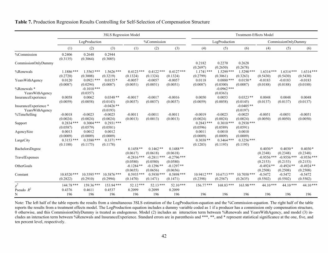
42

Table 7. Production Regression Results Controlling for Self-Selection of Compensation Structure

Note: The left half of the table reports the results from a simultaneous 3SLS estimation of the LogProduction-equation and the %Commission-equation. The right half of the table reports the results from a treatment effects model. The LogProduction equation includes a dummy variable coded as 1 if a producer has a commission only compensation structure, 0 otherwise, and this CommissionOnlyDummy is treated as endogenous. Model (2) includes an interaction term between %Renewals and YearsWithAgency, and model (3) in-cludes an interaction term between %Renewals and InsuranceExperience. Standard errors are in parenthesis and ***, **, and * represent statistical significance at the one, five, and ten percent level, respectively.

3SLS Regression Model Treatment-Effects Model

LogProduction %Commission LogProduction CommissionOnlyDummy

(1) (2) (3) (1) (2) (3) (4) (5) (6) (4) (5) (6)

%Commission 0.2406 0.2648 0.2944 (0.3135) (0.3064) (0.3085) CommissionOnlyDummy 0.2182 0.2270 0.2628 (0.2697) (0.2650) (0.2678) %Renewals 1.1886 *** 1.5563 *** 1.5626 *** 0.4123 *** 0.4122 *** 0.4127 *** 1.1741 *** 1.5299 *** 1.5290 *** 1.6314 *** 1.6314 *** 1.6314 *** (0.2720) (0.3008) (0.3219) (0.1324) (0.1324) (0.1324) (0.2799) (0.3061) (0.3263) (0.5430) (0.5430) (0.5430) YearsWithAgency 0.0120 0.0921 *** 0.0155 * -0.0057 -0.0057 -0.0057 0.0118 0.0880 *** 0.0150 * -0.0183 -0.0183 -0.0183 (0.0087) (0.0294) (0.0087) (0.0051) (0.0051) (0.0051) (0.0087) (0.0300) (0.0087) (0.0188) (0.0188) (0.0188) %Renewals * -0.1010 *** -0.0962 *** YearsWithAgency (0.0357) (0.0363) InsuranceExperience 0.0058 0.0062 0.0348 ** -0.0017 -0.0017 -0.0016 0.0050 0.0053 0.0323 ** 0.0048 0.0048 0.0048 (0.0059) (0.0058) (0.0143) (0.0037) (0.0037) (0.0037) (0.0059) (0.0058) (0.0145) (0.0137) (0.0137) (0.0137) InsuranceExperience * -0.0426 ** -0.0405 ** YearsWithAgency (0.0193) (0.0197) %TimeSelling -0.0018 -0.0023 -0.0025 -0.0011 -0.0011 -0.0011 -0.0019 -0.0023 -0.0025 -0.0051 -0.0051 -0.0051 (0.0024) (0.0024) (0.0024) (0.0013) (0.0013) (0.0013) (0.0024) (0.0024) (0.0024) (0.0050) (0.0050) (0.0050) Support 0.2834 *** 0.3004 *** 0.2931 *** 0.2843 *** 0.3010 *** 0.2938 *** (0.0587) (0.0579) (0.0581) (0.0596) (0.0589) (0.0591) AgencySize 0.0013 0.0012 0.0012 0.0011 0.0010 0.0010 (0.0009) (0.0009) (0.0009) (0.0009) (0.0009) (0.0009) LargeCity 0.3153 *** 0.3580 *** 0.3371 *** 0.3038 ** 0.3464 *** 0.3256 *** (0.1188) (0.1175) (0.1178) (0.1203) (0.1193) (0.1195) BachelorsDegree 0.1458 ** 0.1462 ** 0.1488 ** 0.4030 * 0.4030 * 0.4030 * (0.0617) (0.0618) (0.0618) (0.2348) (0.2348) (0.2348) TravelExpenses -0.2816 *** -0.2811 *** -0.2796 *** -0.9556 *** -0.9556 *** -0.9556 *** (0.0580) (0.0580) (0.0580) (0.2153) (0.2153) (0.2153) OtherGoals -0.1284 ** -0.1296 ** -0.1297 ** -0.4924 ** -0.4924 ** -0.4924 ** (0.0655) (0.0656) (0.0656) (0.2508) (0.2508) (0.2508) Constant 10.8520 *** 10.5595 *** 10.5876 *** 0.5935 *** 0.5930 *** 0.5898 *** 10.9412 *** 10.6713 *** 10.7058 *** -0.5472 -0.5472 -0.5472 (0.2822) (0.2910) (0.2994) (0.1470) (0.1471) (0.1471) (0.2398) (0.2567) (0.2635) (0.5502) (0.5502) (0.5502)

χ2 144.78 *** 159.36 *** 153.94 *** 52.12 *** 52.13 *** 52.10 *** 156.77 *** 168.83 *** 163.98 *** 44.10 *** 44.10 *** 44.10 *** Pseudo R2 0.4376 0.4611 0.4537 0.2099 0.2099 0.2099 N 196 196 196 196 196 196 196 196 196 196 196 196

43

Table 8. 3SLS Regressions of Production, Compensation and Compensation Structure

Note: This table reports the results from a simultaneous 3SLS estimation of the LogProduction-equation, the %Commission-equation, and the LogTotal-Compensation-equation. Model (2) includes an interaction term between %Renewals and YearsWithAgency, and model (3) includes an interaction term be-tween %Renewals and InsuranceExperience. Standard errors are in parenthesis and ***, **, and * represent statistical significance at the one, five, and ten percent level, respectively.

LogProduction %Commission LogTotalCompensation

(1) (2) (3) (1) (2) (3) (1) (2) (3)

LogProduction 0.7872 *** 0.7377 *** 0.7396 *** (0.1126) (0.1032) (0.1050) %Commission 0.2452 0.2649 0.2966 -0.5689 -0.4668 -0.4675 (0.3102) (0.3037) (0.3055) (0.3899) (0.3729) (0.3752) %Renewals 1.1630 *** 1.4889 *** 1.4677 *** 0.4285 *** 0.4187 *** 0.4197 *** (0.2620) (0.2922) (0.3116) (0.1273) (0.1281) (0.1282) YearsWithAgency 0.0121 0.0805 *** 0.0146 * -0.0056 -0.0056 -0.0056 0.0015 0.0032 0.0031 (0.0087) (0.0279) (0.0087) (0.0051) (0.0051) (0.0051) (0.0076) (0.0073) (0.0073) %Renewals * -0.0866 ** YearsWithAgency (0.0338) InsuranceExperience 0.0058 0.0061 0.0289 ** -0.0017 -0.0016 -0.0016 -0.0087 -0.0081 -0.0081 (0.0059) (0.0058) (0.0136) (0.0036) (0.0036) (0.0036) (0.0058) (0.0056) (0.0056) InsuranceExperience * -0.0341 * YearsWithAgency (0.0182) %TimeSelling -0.0022 -0.0025 -0.0026 -0.0009 -0.0009 -0.0009 (0.0023) (0.0023) (0.0023) (0.0012) (0.0013) (0.0013) Support 0.2852 *** 0.3062 *** 0.2995 *** (0.0558) (0.0557) (0.0560) AgencySize 0.0014 0.0013 0.0013 (0.0009) (0.0009) (0.0009) LargeCity 0.3144 *** 0.3493 *** 0.3294 *** 0.0812 0.1011 0.0992 (0.1186) (0.1172) (0.1176) (0.0937) (0.0904) (0.0907) BachelorsDegree 0.1457 ** 0.1458 ** 0.1487 ** 0.2178 ** 0.2106 ** 0.2043 ** (0.0617) (0.0617) (0.0618) (0.0898) (0.0871) (0.0870) TravelExpenses -0.2812 *** -0.2809 *** -0.2793 *** -0.2612 * -0.2292 * -0.2326 * (0.0579) (0.0580) (0.0580) (0.1350) (0.1300) (0.1304) OtherGoals -0.1252 ** -0.1301 ** -0.1295 ** (0.0619) (0.0629) (0.0630) Pension 0.0385 0.0359 0.0434 (0.0848) (0.0840) (0.0844) FirstJob -0.0867 -0.0959 -0.0961 (0.0801) (0.0801) (0.0801) Constant 10.8772 *** 10.6160 *** 10.6515 *** 0.5730 *** 0.5790 *** 0.5752 *** 2.2893 ** 2.7938 *** 2.7748 *** (0.2735) (0.2836) (0.2914) (0.1402) (0.1415) (0.1416) (1.1014) (1.0058) (1.0240)

χ2 144.94 *** 159.75 *** 154.71 *** 52.38 *** 51.96 *** 51.95 *** 153.99 *** 163.19 *** 161.53 ***Pseudo R2 0.4378 0.4605 0.4531 0.2097 0.2098 0.2098 0.4314 0.4837 0.4827 N 196 196 196 196 196 196 196 196 196

44

Table 9. Blinder-Oaxaca Decomposition of Sales Production Adjusted for Self-Selection

Variable: LogProduction

Predicted value of LogProduction variable for:

Salary Only Producers 12.1523 12.1523

Mixed Pay Producers 12.0243 12.0243

Commission Only Producers 12.5298 12.5298

Difference in predicted values 0.5055(<0.001)

*** 0.3774(0.031)

** -0.1281(0.468)

Adjusted difference 0.4204(0.158)

0.2779(0.407)

0.1981(0.768)

Explained part of difference 0.2957(0.002)

*** 0.1756(0.227)

-0.1431(0.319)

Unexplained part of difference 0.1248(0.696)

0.1023(0.761)

0.3412(0.614)

Note: This table reports the two-fold decomposition of the difference in mean predicted values of LogProduction across compensation types. The difference is adjusted for self-selection of compensation schemes. The decomposi-tion is based on Equation (7) without the %Commission variable, including a correction term for self-selection. Statistical significance of the explained and unexplained parts of the difference are based on Jann’s (2008) test which corrects standard errors for sampling variances. P-values are in parenthesis and ***, **, and * represent sta-tistical significance at the one, five, and ten percent level, respectively.