In Search of Earnings Predictability�

Zhi Day, Joseph Engelbergzand Pengjie Gaox

This Draft: April 9, 2010

First Draft: October 19, 2009

Preliminary and Incomplete

Abstract

We use search volume for a �rm�s products to predict the earnings surprises of that

�rm. We �nd that increases (decreases) in the search volume index (SVI) of a �rm�s

most popular product predict positive (negative) revenue surprises and standardized

unexpected earnings (SUE). SVI also predicts earnings surprises relative to analyst

forecasts and the earnings announcement return. Taken together, the evidence suggests

that search volume for a �rms�products is a value-relevent leading indicator that the

market does not fully incorporate into its expectations of earnings.

�We thank Nielsen Media Research for providing data in this study. We thank seminar participants atthe University of Notre Dame, Peter Easton and Paul Tetlock for helpful comments and suggestions. Weare responsible for remaining errors.

yFinance Department, Mendoza College of Business, University of Notre Dame. E-mail: zda@nd.edu;Tel: (574) 631-0354.

zFinance Department, Kenan-Flagler Business School, University of North Carolina at Chapel Hill. E-mail: joseph_engelberg@kenan-�agler.unc.edu; Tel: (919) 962-6889.

xFinance Department, Mendoza College of Business, University of Notre Dame. E-mail: pgao@nd.edu;Tel: (574) 631-8048.

�. . . if you can assemble a diverse group of people who possess varying degrees

of knowledge and insight, you�re better o¤ entrusting it with major decisions

rather than leaving them in the hands of one or two people, no matter how

smart those people are.�

� James Surowiecki, The Wisdom of Crowds

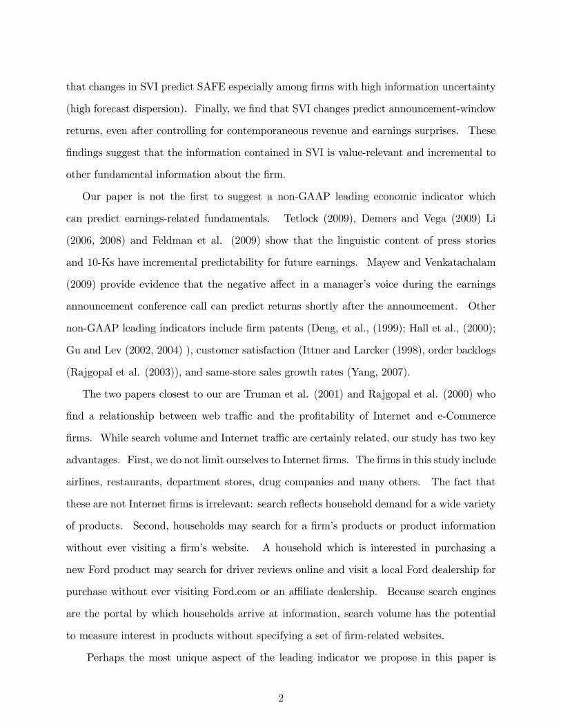
1 Introduction

Search queries re�ect the intentions of those who query. For example, when search volume

for a brand of automobile is high, sales for that brand of auto are also high. Therefore,

when economic data are released with a lag, search volume may be able to predict the

content of these lagged releases. According to Choi and Varian (2009) �query data may

be correlated with the current level of economic activity in given industries and thus may

be helpful in predicting the subsequent data releases.� Choi and Varian (2009) support

this claim by providing evidence that search volume can predict subsequent reports of home

sales, automotive sales and tourism.

Because search data appear well-suited to predict lagged releases of economic activity,

here we consider the predictability of search volume for �rm earnings announcements. Firms

report earnings information with a lag four times a year. This paper examines whether search

volume can predict the content of these announcements. We have four key �ndings. First,

we �nd that the search volume index (SVI) of a �rm�s most popular product is related to

the revenue announced by the �rm. Increases (decreases) in SVI strongly predict positive

(negative) revenue surprises for the �rm on its announcement day. This result holds even

after including a host of controls that have been shown to predict revenue surprises in

previous research. Second, this predictability also holds for the earnings per share of the

�rm: changes in SVI predict standardized unexpected earnings (SUE). Third, when we

consider the earnings surprise relative to the consensus analyst forecast (SAFE), we �nd

1

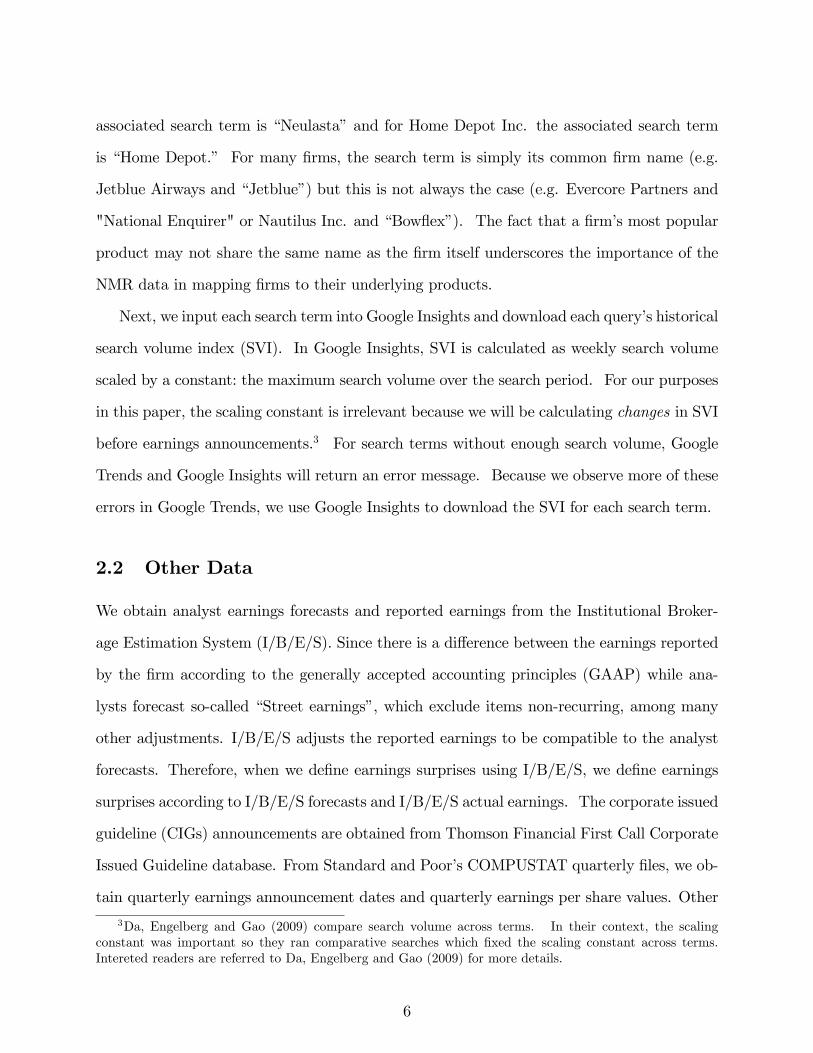
that changes in SVI predict SAFE especially among �rms with high information uncertainty

(high forecast dispersion). Finally, we �nd that SVI changes predict announcement-window

returns, even after controlling for contemporaneous revenue and earnings surprises. These

�ndings suggest that the information contained in SVI is value-relevant and incremental to

other fundamental information about the �rm.

Our paper is not the �rst to suggest a non-GAAP leading economic indicator which

can predict earnings-related fundamentals. Tetlock (2009), Demers and Vega (2009) Li

(2006, 2008) and Feldman et al. (2009) show that the linguistic content of press stories

and 10-Ks have incremental predictability for future earnings. Mayew and Venkatachalam

(2009) provide evidence that the negative a¤ect in a manager�s voice during the earnings

announcement conference call can predict returns shortly after the announcement. Other

non-GAAP leading indicators include �rm patents (Deng, et al., (1999); Hall et al., (2000);

Gu and Lev (2002, 2004) ), customer satisfaction (Ittner and Larcker (1998), order backlogs

(Rajgopal et al. (2003)), and same-store sales growth rates (Yang, 2007).

The two papers closest to our are Truman et al. (2001) and Rajgopal et al. (2000) who

�nd a relationship between web tra¢ c and the pro�tability of Internet and e-Commerce

�rms. While search volume and Internet tra¢ c are certainly related, our study has two key

advantages. First, we do not limit ourselves to Internet �rms. The �rms in this study include

airlines, restaurants, department stores, drug companies and many others. The fact that

these are not Internet �rms is irrelevant: search re�ects household demand for a wide variety

of products. Second, households may search for a �rm�s products or product information

without ever visiting a �rm�s website. A household which is interested in purchasing a

new Ford product may search for driver reviews online and visit a local Ford dealership for

purchase without ever visiting Ford.com or an a¢ liate dealership. Because search engines

are the portal by which households arrive at information, search volume has the potential

to measure interest in products without specifying a set of �rm-related websites.

Perhaps the most unique aspect of the leading indicator we propose in this paper is

2

its source. Intuitively, there are two natural sources for leading indicators of earnings:

�rms and customers. Consider, for example, the �rm Apple Inc. which sells Ipods to

millions of customers and then announces the sales at some later date (e.g. the �earnings

announcement�). Each customer is partially informed about Apple�s sales: they each know

of their own purchase and little else. Apple may be fully informed of its sales and, for

this reason, the most popular leading indicators originate from the �rm (e.g., Feldman et al

(2009), Demers and Vega (2009), Deng, et al. (1999); Hall et al. (2000); Gu and Lev (2002,

2004), Mayew and Venkatachalam (2009), Rajgopal et al. (2003); Yang (2007)).

This paper proposes a leading indicator which originates from the customers. Consider

again the millions of customers who buy Ipods. Now suppose these customers search for

Ipods online in a search engine like Google before executing their purchases. Then by

aggregating the search volume for Ipods, the search engine can coordinate the information

of each customer. In the extreme case where every Ipod customer searches for an Ipod before

making his purchase, search volume will perfectly signal Apple�s future announcement of Ipod

sales.

The customer-based leading indicator we propose has several advantages over a �rm-

based one. First, search volume data are reported and updated daily, while most leading

indicators are released sporadically throughout the year. The real-time nature of search

volume not only allows information producers to constantly update but it also allows for

event-time analysis for products that have speci�c release dates. For example, Microsoft

released Windows 7 on October 22, 2009. A real-time indicator such as search volume allows

information producers to estimate demand around the release date. Second, search volume is

produced by a third-party and is therefore less likely to be biased. Most leading indicators are

released by �rms who may have an incentive to spin or selectively disclose information most

favorable to the �rm (Dyck and Zingales (2004)). Finally, a customer-based leading indicator

may even be useful to �rms. Along the chain of suppliers and customers, information does

not transmit without friction or delay. Thus, even a �rm�s manager may not necessarily

3

observe all the customer�s detailed product level demand information. In summary, the

product search volume data have the potential to provide value-relevant information about

the �rm on a real-time basis.

Some of these advantages have already been recognized in papers which have used search

volume to measure household demand for a variety of information. Ginsberg et al. (2008)

found that search data for forty-�ve terms related to in�uenza predicted �u outbreaks one

to two weeks before Centers for Disease Control and Prevention (CDC ) reports. The

authors conclude that, �harnessing the collective intelligence of millions of users, Google

web search logs can provide one of the most timely, broad-reaching in�uenza monitoring

systems available today.� More recently, Da, Engelberg and Gao (2009) examined search

volume for stock tickers (e.g., �MSFT�and �AAPL�). They provide evidence that stock-

ticker search volume re�ects retail demand for shares and has predictability for short-term

returns, especially among small stocks.

The rest of the paper is organized as follows. Section 2 describes our data sources and

the way in which we construct the SVI for �rm products. In Section 3, we use the product-

level SVI to predict �rm revenue surprises. Section 4 provides evidence that SVI predicts

standardized unexpected earnings (SUE). Section 5 considers how SVI predicts earnings

surprises from analysts forecasts. Section 6 examines predictability for returns around the

earnings announcement. Finally, Section 7 concludes.

2 Data and Sample Construction

2.1 Main Data

Because we wish to estimate household demand for �rm products, our �rst challenge is to

obtain a list of products for each �rm. We begin by gathering data on �rm products from

4

Nielsen Media Research (NMR) which tracks television advertising for �rms.1 NMR provided

to us a list of all �rms which advertised a product on television during our time period of

2004 - 2008. From this list of 9,764 unique �rms, we hand-match the set of �rms which

are publicly traded to COMPUSTAT�s unique identi�er (GVKEY). This results in a list of

865 �rms. For those unmatched �rms, nearly all of them are private �rms (e.g., the Law

O¢ ces of James Sokolove; Empire Today and City Mattress) or non-pro�t organizations

(e.g., Habitat for Humanity; the American Red Cross and the Public Broadcasting Service).

Our sample of 865 �rms are associated with 12,259 brand/products in the Nielsen data-

base. Some �rms have hundreds of products while others have very few products. For

example, Time Warner Inc. has 886 products in the database, ranging from magazines such

as People to home videos such as seasons of Friends and the West Wing. On the other

hand, Lojack Inc. only advertises one product: its Lojack Security System. In fact, there

are 337 �rms which only advertise one product according to NMR.

To make our data collection process manageable, for each �rm we select its most popular

product as measured by the number of ads in the Nielsen database. Then, we consider how

these 865 products might be searched in Google. We do this by having two independent

research assistants report how they would search for each product. Where there are dif-

ferences between the reports, we use Google Insights �related search�feature to determine

which query is most common.2

The resulting database is a list of �rms associated with search terms for their most

popular product. Table 1 provides a random sample of 75 �rms and their associated search

term. For example, for Apple Inc. the associated search term is �Ipod�, for Amgen Inc the

1Using detailed corporate level advertisement information is relatively new in the accounting literature.Cohen, Mashruwala and Zach (2009) use a database from an anonymous data vendor to track corporatemonthly advertisement spending and explore managerial discretion in real earnings management. However,we are not aware of any prior studies using Nielson Media Research�s product-level advertisement datasetused in this paper.

2For each term entered into Google Insights (http://www.google.com/insights/) it returns ten �topsearches� related to the term. According to Google, �Top searches refer to search terms with the mostsigni�cant level of interest. These terms are related to the term you�ve entered. . . our system determinesrelativity by examining searches that have been conducted by a large group of users preceding the searchterm you�ve entered, as well as after."

5

associated search term is �Neulasta�and for Home Depot Inc. the associated search term

is �Home Depot.� For many �rms, the search term is simply its common �rm name (e.g.

Jetblue Airways and �Jetblue�) but this is not always the case (e.g. Evercore Partners and

"National Enquirer" or Nautilus Inc. and �Bow�ex�). The fact that a �rm�s most popular

product may not share the same name as the �rm itself underscores the importance of the

NMR data in mapping �rms to their underlying products.

Next, we input each search term into Google Insights and download each query�s historical

search volume index (SVI). In Google Insights, SVI is calculated as weekly search volume

scaled by a constant: the maximum search volume over the search period. For our purposes

in this paper, the scaling constant is irrelevant because we will be calculating changes in SVI

before earnings announcements.3 For search terms without enough search volume, Google

Trends and Google Insights will return an error message. Because we observe more of these

errors in Google Trends, we use Google Insights to download the SVI for each search term.

2.2 Other Data

We obtain analyst earnings forecasts and reported earnings from the Institutional Broker-

age Estimation System (I/B/E/S). Since there is a di¤erence between the earnings reported

by the �rm according to the generally accepted accounting principles (GAAP) while ana-

lysts forecast so-called �Street earnings�, which exclude items non-recurring, among many

other adjustments. I/B/E/S adjusts the reported earnings to be compatible to the analyst

forecasts. Therefore, when we de�ne earnings surprises using I/B/E/S, we de�ne earnings

surprises according to I/B/E/S forecasts and I/B/E/S actual earnings. The corporate issued

guideline (CIGs) announcements are obtained from Thomson Financial First Call Corporate

Issued Guideline database. From Standard and Poor�s COMPUSTAT quarterly �les, we ob-

tain quarterly earnings announcement dates and quarterly earnings per share values. Other

3Da, Engelberg and Gao (2009) compare search volume across terms. In their context, the scalingconstant was important so they ran comparative searches which �xed the scaling constant across terms.Intereted readers are referred to Da, Engelberg and Gao (2009) for more details.

6

accounting information is obtained from COMPUSTAT annual �les.

Table 2 presents some summary statistics (mean, median and standard deviation) for

these variables and compares and compares them to the CRSP/COMPUSTAT universe

over our sample period (2004 - 2008). On average, �rms that advertise on national TV

are larger �rms with higher turnover and lower Market-to-Book ratios. While our sample

of �rms are likely to tilt towards larger and growth �rms, in terms of revenue surprise or

earnings surprises, as well as past return performance, there is no noticeable and economically

signi�cant di¤erence. For instance, for our sample of �rm, the earnings surprise (measured

from the time-series model) is about 0.144 to 0.146, while the COMPUSTAT/CRSP universe

is about 0.141 to 0.143. The average analyst earnings forecast surprise in our sample is about

0.045, and the average forecast surprise in the COMPUSTAT/CRSP universe is about 0.041.

2.3 Examples

Figure 1 provides a sample of our data for two �rms: Garmin LTD (search term �Garmin�)

and CEC Entertainment (search term �Chuck E Cheese�). The SVI for �Garmin�indicates

a rapid growth in interest for Garmin products, consistent with the rapid growth in GPS

navigation products. On the other hand, the SVI for �Chuck E Cheese�indicates very little

growth between 2004 and 2007 and some modest growth beginning in 2008. The SVI for

�Chuck E Cheese�appears to have more seasonality than the SVI for �Garmin.� Turning

to the earnings of Garmin LTD and CEC Entertainment in Figure 2, we see that the SVI for

their products closely follows the reported earnings. Of course, these anecdotes are simply

illustrations. In the next section we begin a more rigorous examination of the predictability

of SVI for �rm fundamentals.

7

3 Predicting Revenue Surprises

We begin our analysis of the relationship between search volume and �rm fundamentals where

we expect it to be strongest: sales. Indeed, if households search for a product before their

purchase, we should �nd a strong relationship between search patterns and sales patterns

(Choi and Varian (2009)).

Predicting such sales patterns is a worthwhile endeavor. From a practical point of view,

revenue or sales forecasts are important for both market participants and �rm managers.

First, revenue forecasts are ingredients of �nancial statement analysis. Sound investment

recommendations and decisions partially depend on sound revenue or sales forecasts. Ulti-

mately, a company�s earnings derive from sales less costs. For many modern �rms, especially

those outside basic materials sector, input prices are relatively sticky because long-term con-

tracts or competitive procurement processes. Thus, the cost structure is relatively stable and

easy to forecast. However, the demand-side forces, i.e., revenue or sales, are more volatile.

Therefore, not surprisingly, sales volatility drives earnings volatility for many �rms. Second,

revenue forecasts are crucial inputs for �rm managers to make internal capital allocation

decisions, even though managers are supposed to have better access to product-level sales

information. In reality, because the retailers, wholesalers and manufacturers are not per-

fectly integrated in sharing information, sales information is not readily available to most

managers in real time.

According to Lundholm, McVay and Randall (2009), there is �surprisingly little�account-

ing research on forecasting of sales and revenues. Recent literature (Ertimur, Livant, and

Martikainen, 2003; Jegadeesh and Livnat, 2006; Ghosh, Gu, and Jain, 2005) �nds revenues

and revenue surprises convey incremental information about earnings and market valuation.

However, there is little research exploring the relationship between non-�nancial information

and revenue surprises. In other words, it is not clear whether non-�nancial information in

a general setting is able to provide incremental information about revenue surprises. In this

section, we provide strong evidence that search volume forecasts revenue surprises.

8

Following Jegadeesh and Livnat (2006), for each �rm in each quarter we de�ne revenue

surprise as

SUSi;q;k =REVi;q �REVi;q�k

� (REVi)

where REVi is the quarterly sales (in dollar value) reported by �rm i, REVi;q�k is �rm i�s

quarterly sales reported k periods ago and � (REVi) is the standard deviation of revenue

during the past eight quarters. We consider both k = 1 and k = 4 in our analysis. When

k = 1, the (naive) expectation of sales is that of the previous quarter; when k = 4, revenue

surprises are seasonally adjusted.4

For each �rm in each quarter we de�ne the change in search volume as:

SV I_Changei;q;k = log(SV Ii;q)� log(SV Ii;q�k)

where SV Ii;q is the average weekly search volume index for �rm i during quarter q.

Table 3 considers a regression of SUSi;q;k on SV I_Changei;q;k and a series of control

variables. The top panel considers last quarter�s sales as the expectation (k = 1) while the

bottom panel considers sales four quarters ago as the expectation (k = 4). Each speci�cation

includes GIC sector �xed e¤ects and year �xed e¤ects.

The �rst column of the top panel demonstrates that SV I_Changei;q;1 has strong pre-

dictability for SUSi;q;1:A one standard deviation increase in SV I_Changei;q;1 corresponds

to an increase in standardized unexpected revenues by :20 (t-stat = 9:86).

Beginning in column two, the top panel adds a series of control variables including size,

market-to-book, turnover, historical return, and institutional ownership. Each has a negli-

gible e¤ect on the variable of interest.

As our leading indicator originates from customers rather than �rms, we control for

management forecasts in column 7. Management�s discretionary disclosure policy a¤ects

4As a robustness check, for each �rm in each quarter we construct its Sales_Growthi;q:q�1 de�nedas the percentage change in sales between quarter q and quarter q � 1 for �rm i. We also constructSales_Growthi;q:q�4 to take into account the seasonality in sales. Using these alternative de�nitions ofrevenue growth, we obtain very similar results.

9

the analyst choice of whether to cover the �rm, which in turn a¤ects a �rm�s information

environment (Lang and Lundholm, 1996). In addition, managers may guide the analysts

in making earnings forecasts through the earning cycle (Cotter, Tuna, and Wysocki, 2006).

From the First Call Corporate Issued Guideline database, we count the number of manage-

ment issued guidelines related to quarterly earnings between two quarters. Management

forecasts also have strong predictability for revenue surprises with coe¢ cients that have

the predicted sign: the number of positive (negative) management forecasts has a positive

(negative) e¤ect on SUSi;q;1. Nevertheless, the coe¢ cient on SV I_Changei;q;1 remains

economically and statistically signi�cant (t-stat of 9:98).

The �nal speci�cation (column 8) adds lagged revenue surprise as an independent vari-

able. Controlling for the (non seasonally-adjusted) lagged revenue surprise actually increases

the coe¢ cient on SV I_Changei;q;1 from :875 to :919.

While the previous results suggest that search volume correlates well with sales, we do

not know whether this e¤ect is due to seasonality. For example, a retailer�s sales are often

high during the holiday season, and so is search volume for its products. The bottom panel

asks whether search volume has predictability for sales beyond seasonality. For example,

can search volume predict whether a retailer�s sales this holiday season will be better than

the prior one?

The evidence suggests "yes." The bottom panel of Table 3 regresses seasonally-adjusted

revenue surprises (SUSi;q;4) on seasonally-adjusted search volume (SV I_Changei;q;4). Nev-

ertheless, the coe¢ cient on SV I_Changei;q;4 is large (:487) and statistically signi�cant (t-

stat of 5:17). As in the top panel, we add control variables one at a time in each speci�cation.

In the last speci�cation, we control for the (seasonally-adjusted) lagged revenue surprise.

The coe¢ cient on lagged (seasonally-adjusted) revenue surprise is large and signi�cant, con-

sistent with prior work that �nds a strong autocorrelation in revenue surprises (Jegadeesh

and Livnat (2006)). The presence of lagged revenue surprise reduces the coe¢ cient on

SV I_Changei;q;4 from .357 to .116, but it remains signi�cant (t-stat of 2:43).

10

4 Predicting Earnings Surprises

Earnings announcements convey important incremental information to �nancial markets.

Beaver (1968) and Ball and Shivakumar (2008), among others provide evidence that infor-

mation revealed by quarterly earnings announcements is useful to shareholders. Similarly,

Easton, Monahan, and Varsvari (2009) study investors reaction in the bond market to quar-

terly earnings announcements. Earnings announcements also change the expectations of

investors as demonstrated by Lakonishock, Shleifer and Vishny (1994) and Skinner and

Sloan (2002). Given the importance and prevalence of earnings announcements, a large

body of literature has been developed to study earnings surprises.

In the previous section, we provided evidence that innovations in search volume had pre-

dictability for revenue surprises. In this section, we ask whether this predictability extends

to earnings surprises. Again, the answer appears to be �yes�, although the relationship is

weaker. This is not surprising as search volume may be directly related to revenue but not

to costs.

We follow Livnat and Mendenhall (2006) and calculate the random-walk version of stan-

dardized unexpected earnings (SUE). Speci�cally, SUEi;q is the change in earnings per

share between quarter q and quarter q � 4 for �rm i scaled by the price per share:

SUEi;q;4 =EPSi;q � EPSi;q�4

Pi;q�4:

Table 4 reports the results of two regressions which regress SUEi;q;4 on SV I_Changei;q;4.

The full set of controls used in column 8 of Table 3 are deployed here except that we replace

lagged revenue surprise with lagged SUE in these speci�cations. In the �rst column of Table

4, SUE is calculated without excluding extraordinary items whereas in the second column

we exclude extraordinary items as in Livnat and Mendenall (2006). As expected, search

volume has a weaker relationship with earnings than it does with sales.

There are several ways to look at these results. First, these results may be related to

11

corporate�s decisions on earnings smoothing and choice of accruals. In untabulated results,

we have also considered the possibility that SV I_Change is a proxy for accruals. If accruals

exhibit a mean reverting tendency (Sloan, 1996), future earnings surprises are related to past

accrual decisions. Although we �nd a positive coe¢ cient on lagged accruals, in our sample

it is neither economically or statistically signi�cant. Again, after including accruals in the

regression, the relationship between SV I_Change and SUE remains qualitatively similar.

Second, these results may also be consistent with the view that earnings numbers �by

numerical value itself �do not convey all value-relevant accounting information, especially

at the quarterly frequency. Put di¤erently, the value-relevance of non-�nancial information

may be related to earnings numbers but goes beyond the earnings number. We explore this

point further in the following sections.

5 SVI and Analyst Forecasts

In the previous section we found evidence that SV I_Changei;q;4 predicts earnings surprises

as calculated from a simple time-series model. The model, however, does not capture

additional information analysts may have beyond last year�s earnings per share. In order to

measure earnings surprise relative to analysts�forecasts, we de�ne SAFEi;q:

SAFEi;q =EPSi;q �Med(AFi;q)

Pi;q�4:

whereMed(AFi;q) is the median analyst forecast taken from I/B/E/S summary �les for �rm

i in quarter q.

In Table 5, we report a series of regressions where the standardized analyst forecast

error, SAFEi;q, is the dependent variable and SV I_Changei;q;4 is the independent variable.

Each regression includes the control variables of Table 4. The �rst column shows a positive,

albeit weak relationship between SAFE and SV I_Change (coe¢ cient of :098 and t-stat =

1:89). The fact that SV I_Change is a stronger predictor of revenue surprise and SUE but

12

a weaker predictor of SAFE is consistent with the notion that, on average, analysts have

some information contained in SV I_Change.

However, there is large cross-sectional variation in the information environment of �rms.

While, on average, analysts may have the information which coincides with the information

content of SV I_Change, for a set of �rms with opaque or complex information environment,

the information content of SV I_Change may be particularly important. For example,

Jiang, Lee and Zhang (2005), and Zhang (2006a, 2006b) suggest that information uncertainty

plays an important role in the aggregation of information. High information uncertainty

potentially contributes to and exacerbates the biased estimates of fundamental value of a

stock, because the feedback on valuation is particularly slow in an environment with high

level of information uncertainty. In particular, Zhang (2006b) documents stronger analyst

forecast ine¢ ciency - stronger autocorrelations of forecast errors - among set of �rms with

higher information uncertainty. They use several variables, such as �rm age, trading volume,

size, and forecast dispersion in delineating the information uncertainty. Since �rms in our

sample are usually large and mature, some of these proposed proxy variables do not generate

economically meaningful cross-sectional dispersions for carrying out statistically powerful

tests. Thus, we choose to focus on a simple measure, analyst forecast dispersion, in our

empirical analysis.

We follow Diether, Malloy and Scherbina (2002) and use the dispersion of analyst forecasts

as a measure of the information uncertainty. When we sort �rms based on their meaures of

analyst dispersion, we �nd strong di¤erential performance of SV I_Change for predicting

SAFE. The second column of Table 5 repeats the speci�cation of column 1 only among

�rms below the median analyst forecast dispersion. The third column of Table 5 repeats

the speci�cation of column 1 only among �rms above the median analyst forecast dispersion.

The di¤erence is striking: only among the set of �rms with large information uncertainty

(high forecast dispersion) do we �nd a positive and signi�cant e¤ect. In fact, among the set

of �rms with low forecast dispersion, the coe¢ cient is actually negative (�:017) although

13

insigni�cant (t-stat of �1:16).

Taken together, these results suggest that SVI may be a useful forecasting tool for an-

alysts, especially when information about earnings is di¢ cult to acquire. Meanwhile, these

results also suggest that sell-side analysts exhibit some ability in incorporating product level

information into their earnings forecast, though incorporation of such information is incom-

plete among the set of �rms where the information uncertainty is particularly high.

6 SVI and Announcement Returns

Motivated by our previous �nding that analysts may not have some information contained

in search volume, here we examine whether search volume can predict the market response

around earnings announcements. There are several reasons to believe information contained

in search volume is value-relevant and may predict announcement returns. First, the infor-

mation contained in search volume is not found in other places. Beyond aggregate sales and

to a lesser extent the sales by geographical segments, �rms usually do not disclose detailed

product level information. However, as illustrated in Boatsman, Behn, and Patz (1993),

disaggregate information such as sales by geographic segments is value-relevant. Second,

a key di¤erence between earnings surprise as measured by analysts or a time-series model

and surprise as measured by announcement return is that only the latter is forward-looking.

Returns incorporate future information about fundamentals and there is good reason to be-

lieve that the information in search contains forward-looking information: customers search

for information about products before executing their purchase.

To measure the market response, we take the standard approach and calculate cumulative

abnormal returns (CARs) over the three-day window surrounding the earnings announce-

ment. Abnormal return is calculated as the raw daily return from CRSP minus the daily

return on size and market-to-book matched portfolio as in Livnat and Mendenhall (2006).

All CARs are in basis points. Formally we de�ne the abnormal return for �rm i, t days

14

after its quarter q earnings announcement as:

CARi;q;t = Ri;q;t �BRi;q;t

where Ri;q;t is the for �rm i, t days after its quarter q earnings announcement and BRi;q;t is

the size and book-to-market matched �benchmark portfolio�return for �rm i, t days after its

quarter q earnings announcement. Then the announcement-window cumulative abnormal

return for �rm i in quarter q is computed as

CARi;q =1Y

t=�1(1 +Ri;q;t)�

1Yt=�1

(1 +BRi;q;t):

Table 6 reports the results of two regressions which regress CARi;q on SV I_Changei;q;4.

The �rst column, which contains the standard controls as in Table 5, shows a strong relation-

ship between announcement returns and SV I_Change. In fact, is the only variable in the

speci�cation that is signi�cant at the 1% level (t-statistic = 2:64). The economic e¤ects are

also large. A one standard deviation increase in SV I_Change corresponds to an increase

of about 20 basis points over the three-day period (about 17% annualized). Interestingly,

SV I_Change remains a strong predictor of announcement returns even after including the

contemporaneous earnings surprise (column 2) or contemporaneous revenue surprise (column

3).

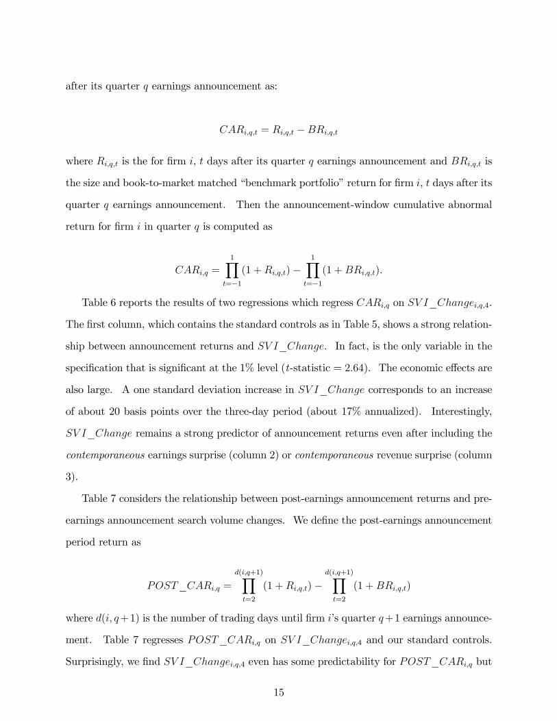
Table 7 considers the relationship between post-earnings announcement returns and pre-

earnings announcement search volume changes. We de�ne the post-earnings announcement

period return as

POST_CARi;q =d(i;q+1)Yt=2

(1 +Ri;q;t)�d(i;q+1)Yt=2

(1 +BRi;q;t)

where d(i; q+1) is the number of trading days until �rm i�s quarter q+1 earnings announce-

ment. Table 7 regresses POST_CARi;q on SV I_Changei;q;4 and our standard controls.

Surprisingly, we �nd SV I_Changei;q;4 even has some predictability for POST_CARi;q but

15

that this is weakened when CARi;q is added to the speci�cation (column 2).

Taken together, the results in Tables 6 and 7 con�rm that changes in product-level

search volume contain substantial value-relevant information that goes beyond quarterly

information released in earnings and revenues.

7 Conclusion

Motivated by other empirical �ndings that search volume is well-suited to predict lagged

releases of economic activity (Choi and Varian, 2009), we use the search volume for a �rm�s

key product to predict revenue and earnings surprises for that �rm. We �nd that increases

(decreases) in the search volume index (SVI) of a �rm�s most popular product predict posi-

tive (negative) revenue surprises and standardized unexpected earnings (SUE). Changes in

search volume also predict earnings surprise relative to the median analyst forecast, espe-

cially among �rms with high information uncertainty. Finally, we �nd strong evidence that

innovations in SVI predict announcement-window abnormal returns, even after controlling

for the earnings and revenue surprise at the announcement. Taken together our �ndings

suggest that search volume for a �rm�s products may be a promising leading indicator for

revenues and earnings announcements of the �rm. Thus, search volume may be a useful

tool for information producers such as analysts and fund managers who are charged with

forecasting �rm fundamentals.

While search volume seems promising as a leading indicator of lagged economic announce-

ments such as earnings announcements, there appears to be no reason why search volume

cannot be applied to other situations. For example, search volume may be particularly

helpful when little information exists to predict sales, as is the case with initial product

launches. Nissan will launch the �rst mass-produced, all-electric vehicle (the Nissan Leaf)

in December 2010 and there is enormous uncertainty about the future demand for this prod-

uct. Search volume seems well-suited for such a situation. By examining the time series

16

of search volume for the Nissan Leaf leading up to the December launch and by compar-

ing search volume for the Nissan Leaf with search volume for other Nissan products where

actual sales are observed, Nissan and its analysts may gather useful information about a

very uncertain outcome. Identifying such key situations in which search volume becomes a

most useful tool for forecasting fundamentals appears to be a promising avenue for future

research.

17

References

Amir, E., and B. Lev, 1996, Value-relevance of Non�nancial Information: The Wireless

Communication Industry. Journal of Accounting and Economics 22, 3�30.

Ball, Ray and Lakshmanan Shivakumar, 2008, How Much New Information is There in

Earnings? Journal of Accounting Research 46, 975-1016.

Beaver, William H, 1968, The Information Content of Annual Earnings Announcements.

Journal of Accounting Research 6, 67-92.

Bernard, V.L., Thomas, J.K., 1989. Post-earnings-announcement drift: delayed price re-

sponse or risk premium?, Journal of Accounting Research 27, 1�36.

Bernard, V.L., Thomas, J.K., 1990. Evidence that stock prices do not fully re�ect the im-

plications of current earnings for future earnings. Journal of Accounting and Economics 13,

305�340.

Boatsman, James R., Bruce K. Behn, and Dennis H. Patz, 1993, A Test of the Use of

Geographical Segment Disclosures, Journal of Accounting Research 31, 46�64.

Choi, H., and H. Varian, 2009, Predicting the Present with Google Trends. Technical Report,

Google Inc.

Cohen, Daniel, Raj Mashruwala, and Tzachi Zach, 2009, Review of Accounting Studies,

Forthcoming.

Cotter, J., T. Irem, and P. Wysocki, 2006, Expectations Management and Beatable Targets:

How Do Analysts React to Explicit Earnings Guidance?. Contemporary Accounting Research

23, 593-624.

Da, Z., and J. Engelberg, and P. Gao, 2009, In Search of Attention.Working Paper, Univer-

sity of Notre Dame and University of North Carolina at Chapel Hill.

Diether, K., C. J. Malloy, and A. Scherbina, 2005, Di¤erences of Opinion and the Cross

Section of Stock Returns, Journal of Finance 57, 2113-2141.

Demers, E. A., and C. Vega, 2009, Soft Information in Earnings Announcements: News or

Noise? Working Paper, INSEAD.

Deng, Z., Lev, B., and Narin, F. ,1999, Science and technology as predictors of stock perfor-

mance, Financial Analysts Journal 55, 20�32.

18

Dyck, A., and L. Zingales, 2004, Private Bene�ts of Control: An International Comparison.

Journal of Finance 59, 537-600.

Easton, Peter D., Steven J. Monahan, and Florin J. Varsvari, 2009, Initial Evidence on

the Role of Accounting Earnings in the Bond Market, Journal of Accounting Research 47,

721�766.

Ertimur, Y., Livnat, J., Martikainen, M., 2003. Di¤erential market reactions to revenue and

expense surprises. Review of Accounting Studies 8, 185�211.

R. Feldman, S. Govindaraj, J. Livnat and B. Segal, 2009, Management�s Tone Change, Post

Earnings Announcement Drift and Accruals, Review of Accounting Studies, Forthcoming.

Ghosh, E., Gu, Z., Jain, P.C., 2005. Sustained earnings and revenue growth, earnings quality,

and earnings response coe¢ cients. Review of Accounting Studies 10, 33�57.

Ginsberg, Jeremy, Matthew H. Mohebbi, Rajan S. Patel, Lynnette Brammer, Mark S.

Smolinski, and Larry Brilliant, 2009, Detecting in�uenza epidemics using search engine query

data, Nature 457, 1012-1014.

Gu, F., and B. Lev, 2002, On the Relevance and Reliability of R&D. Working Paper, Stern

School of Business, New York University.

Gu, F., and B. Lev, 2004, The Information Content of Royalty Income. Accounting Horizons

18, 1�12.

Hall, B., A. Ja¤e and M. Trajtenberg, 2000, Market Value and Patent Citations: A First

Look. Working Paper no. 7741, National Bureau of Economic Research.

Jegadeesh, N., J. Kim, S. Krische, and C. Lee, 2004, Analyzing the analysts: When do

recommendations add value? Journal of Finance 59, 1083-1124.

Jegadeesh, Narasimhan, and Joshua Livnat, 2006, Revenue surprises and stock returns,

Journal of Accounting & Economics 41, 147-171.

Jiang, Guohua, Charles M. C. Lee, and Yi Zhang, 2005, Information Uncertainty and Ex-

pected Returns, Review of Accounting Studies 10, 185� 221.

Lakonishok, J., A. Shleifer and R. Vishny, 1994, Contrarian Investment, Extrapolation, and

Risk, Journal of Finance 49, 1541�1578.

Lang, M. H., and R. J. Lundholm, 1996, Corporate Disclosure Policy and Analyst Behavior.

Accounting Review 71, 467-492.

19

Li, F., 2006, Do Stock Market Investors Understand the Risk Sentiment of Corporate Annual

Reports?, Working Paper, University of Michigan.

Li, F., 2008, Annual Report Readability, Current Earnings, and Earnings Persistance, Jour-

nal of Accounting and Economics 45, 221-247.

Livnat, J., and R. Mendenhall, 2006, Comparing the Post�Earnings Announcement Drift

for Surprises Calculated from Analyst and Time Series Forecasts, Journal of Accounting

Research 44, 177-205.

Livnat, J., and R. Mendenhall, 2006, Comparing the Post�Earnings Announcement Drift

for Surprises Calculated from Analyst and Time Series Forecasts, Journal of Accounting

Research 44, 177-205.

Lundholm, Russell J., Sarah E. McVay, and Taylor Randall, 2009, Forecasting Sales: A

Model and Some Evidence from the Retail Industry, Working Paper, University of Utah.

Mayew, W.J., and M. Venkatachalam, 2009, The power of voice: managerial a¤ective states

and future �rm performance. Working paper, Duke University.

Rajgopal, S., S. Kotha and M. Venkatachalam 2000, The Relevance of Web Tra¢ c for

Internet Stock Prices, Working Paper, University of Washington.

Rajgopal, S., T. Shevlin and M. Venkatachalam, 2003, Does the Stock Market Fully Ap-

preciate the Implications of Leading Indicators for Future Earnings? Evidence from Order

Backlog. Review of Accounting Studies 8, 461�492.

Skinner, Douglas J., and Richard G. Sloan, 2002, Earnings Surprises, Growth Expectations,

and Stock Returns or Don�t Let an Earnings Torpedo Sink Your Portfolio, Review of Ac-

counting Studies 7, 289�321.

Sloan, R. G., 1996, Do Stock Prices Fully Re�ect Information in Accruals and Cash Flows

about Future Earnings?, Accounting Review 71, 289-315.

Tetlock, Paul C., Maytal Saar-Tsechansky, and Sofus Macskassy, 2008, More Than Words:

Quantifying Lanaguage to Measure Firms�Fundamental, Journal of Finance 63, 1437-1467.

Trueman Brett, M. H. Franco Wong, and Xiao-Jun Zhang, 2001, Back to Basics: Forecasting

the Revenues of Internet Firms, Review of Accounting Studies 6, 305�329.

Trueman Brett, M. H. Franco Wong, and Xiao-Jun Zhang, 2000, The Eyeballs Have It:

Searching for the value in Internet Stocks, Journal of Accounting Research 38, 137�162.

20

Yang, Halla, 2007, Do Industry-Speci�c Performance Measure Predict Returns? The Case

of Same-Store Sales, Working Paper, Goldman Sachs Assets Management.

Zhang, X. Frank, 2006, Information Uncertainty and Stock Returns, Journal of Finance

61(1), 105� 137

Zhang, X. Frank, 2006, Information Uncertainty and Analyst Forecast Behaviors, Contem-

porary Accounting Research 23(2), 565� 590.

21

22

Figure 1: Search Volume Index (SVI) for “GARMIN” and “CHUCK E CHEESE”

The figures are screenshots taken from Google Insights (http://www.google.com/insights/). The top

panel plots the search volume index (SVI) for the term “GARMIN” from March 2004 to October 2009. The bottom panel plots the search volume for the term “CHUCK E CHEESE” over the same time period.

23

Figure 2: EPS and SVI for “GARMIN” and “CHUCK E CHEESE”

The figures plot quarterly search volume index (SVI) and earnings per share (EPS) for Garmin LTD (search term “GARMIN”) and CEC Entertainment Inc (search term “CHUCK E CHEESE”).

0

0.2

0.4

0.6

0.8

1

1.2

1.4

1.6

20

25

30

35

40

45

50

55

60

65

Mar

-04

Jun

-04

Sep

-04

De

c-0

4

Mar

-05

Jun

-05

Sep

-05

De

c-0

5

Mar

-06

Jun

-06

Sep

-06

De

c-0

6

Mar

-07

Jun

-07

Sep

-07

De

c-0

7

Mar

-08

Jun

-08

Quarter

Garmin SVI and EPS

Search Volume Index

Earnings Per Share

-0.1

0.1

0.3

0.5

0.7

0.9

1.1

1.3

25

30

35

40

45

50

55

60

65

Mar

-04

Jun

-04

Sep

-04

De

c-0

4

Mar

-05

Jun

-05

Sep

-05

De

c-0

5

Mar

-06

Jun

-06

Sep

-06

De

c-0

6

Mar

-07

Jun

-07

Sep

-07

De

c-0

7

Mar

-08

Jun

-08

Quarter

Chuck E Cheese SVI and EPS

Search Volume Index

Earnings Per Share

24

Table 1: Sample of Firms and Search Terms

The table presents a sample of 75 firms and the associated search quer ies. The query is based on the most popular product as determined by advertising statistics kept by the Nielsen Media Research.

Firm Search Term Firm Search Term Firm Search Term

A M R CORP AMERICAN AIRLINES

HANESBRANDS INC PLAYTEX

MIDAS INC MIDAS SHOP

ALLERGAN INC RESTASIS

HOME DEPOT INC HOME DEPOT

NAUTILUS INC BOWFLEX

AMGEN INC NEULASTA

HONDA MOTOR LTD HONDA

NETFLIX INC NETFLIX

APPLE INC IPOD

I H O P CORP NEW APPLEBEES

NEWELL RUBBERMAID SHARPIE

ASHLAND INC VALVOLINE

IAC INTERACTIVE MATCH.COM

NUTRISYSTEM INC NUTRISYSTEM

AUTOZONE INC AUTOZONE

INTUIT INC QUICKEN

OHIO ART CO ETCH A SKETCH

AVAYA INC AVAYA

INVACARE CORP INVACARE

PEPSICO INC GATORADE

BEBE STORES INC BEBE

IROBOT CORP ROOMBA

POPULAR INC ELOAN

BOSTON BEER INC SAMUEL ADAMS

JARDEN CORP FOODSAVER

PRICELINE COM INC PRICELINE.COM

C A INC CA COMPUTER

JETBLUE AIRWAYS JETBLUE

PROCTER & GAMBLE CO FEBREZE

CEC ENTERTAINMENT CHUCK E CHEESE

KIMBERLY CLARK KLEENEX

RC2 CORP BOB THE BUILDER

COCA COLA CO COKE

KNOT INC THE KNOT

RESEARCH IN MOTION BLACKBERRY

CONSECO INC COLONIAL PENN

KOHLS CORP KOHLS

RUBY TUESDAY INC RUBY TUESDAY

DELL INC DELL

KONAMI CORP KONAMI

SARA LEE CORP HILLSHIRE FARMS

DIA MOND FOODS INC EMERALD NUTS

KRAFT FOODS INC OREO

SEPRACOR INC LUNESTA

EA RTHLINK INC PEOPLEPC

KROGER COMPANY FRED MEYER

SUPERVALU INC ALBERTSONS

EBAY INC EBAY

L C A VISION INC LASIKPLUS

TIVO INC TIVO

ECOLAB INC NASCAR AUTOCARE

LEV ITT CORP FLA BOWDEN HOMES

TREE COM INC LENDINGTREE

ENDOCARE INC CRYOCARE

LIZ CLAIBORNE INC LIZ CLAIBORNE

U A L CORP UNITED AIRLINES

EV ERCORE PARTNERS NATIONAL ENQUIRER

LO JACK CORP LOJACK

UNITED ONLINE INC NETZERO

FEDEX CORP FEDEX

MACYS INC MACYS

V F CORP WRANGLER JEANS

GANNETT INC CAREERBUILDER

MASCO CORP DELTA FAUCETS

VIVENDI ACTIVISION

GAP INC OLD NAVY

MCDONALDS CORP MCDONALDS

WYETH ADVIL

GARMIN LTD GARMIN

MERCK & CO INC SINGULAIR

YAHOO INC YAHOO

GENERAL MILLS INC CHEERIOS

MICROSOFT CORP MICROSOFT

YUM BRANDS INC PIZZA HUT

25

Table 2: Summary Statistics

The following table compares the mean, median and standard deviation of several variables. “Sample” refers to the sample of firms used in this study. Size is the natural logarithm of market capitalization in millions. Market -to-Book is the ratio of market to book value. Turnover is the average turnover during the fiscal quarter. Prior return is the return over the fiscal quarter. The number of positive, neutral and negative firm

issued guidelines is the number of management earning forecasts recorded by First Call constituting positive, neutral, or negative surprises. The revenue surprise (not seasonally adjusted) is defined as the difference between quarter (q) and quarter (q -1), div ided by the standard deviation of revenue from (q-8) to (q-1). The revenue surprise (seasonally adjusted) is defined as the revenue difference between quarter (q) and quarter (q -4), div ided by the standard deviation of revenue from (q-8) to (q-1). Time Series Earnings Surprise is the fiscal quarter’s earnings minus the earnings four quarters ago scaled by price; Analyst Earnings Surprise is the fiscal quarter’s earnings minus the median analyst foreca st scaled by price; is the three day cumulative abnormal return (CAR) surrounding the earnings announcement. CAR – Earnings Window is the cumulative abnormal

return (CAR) in basis points for the three days surrounding the earnings announcement while CAR – Subsequent Quarter is the CAR cumulated from two days after an earnings announcement through one day after the next quarterly earnings announcement. All earnings surprise and CAR variables are calculated as in Livnat and Mendenhall (2006).

Sample CRSP/COMPUSTAT Universe

Variable Mean Median St. Deviation Mean Median St. Deviation

Size (natural log) in millions 8.277 8.207 2.258

5.307 5.506 2.896

Market-to-Book 1.605 1.195 2.072 2.815 0.923 10.254

Turnov er 1.946 1.476 1.856

1.701 1.050 3.555

Prior Return 0.022 0.018 0.178 0.024 0.010 0.247

Firm Guidance: Negative 0.076 0 0.265

0.005 0 0.076

Firm Guidance: Neutral 0.132 0 0.338 0.007 0 0.103

Firm Guidance: Positive 0.056 0 0.230

0.002 0 0.053

Rev enue Surprise (seasonally-adjusted) 0.299 0.218 1.336 0.311 0.184 1.353

Rev enue Surprise (not seasonally -adjusted) 0.856 0.827 1.363

0.805 0.765 1.625

Time-Series Earnings Surprise -0.009 0.146 2.266 0.062 0.141 2.917

Time-Series Earnings Surprise (w/o special items) 0.001 0.144 2.020

0.066 0.143 2.666

Analyst Earnings Surprise 0.003 0.045 0.958 -0.040 0.041 1.292

CAR - Earnings Window (in basis points) 28.518 13.231 699.583

3.328 0.474 774.957

CAR - Subsequent Quarter (in basis points) -47.125 -2.164 1619.610 -36.748 -0.385 1909.350

26

Table 3: SVI Change and Revenue Surprises

In the top panel, the dependent variable is the revenue difference between quarter (q) and quarter (q -1), divided by the standard deviation of revenue from (q-8) to (q-1). In the bottom panel it is the revenue difference between quarter (q) and quarter (q -4), divided by the standard deviation of revenue from (q-8) to (q-1). SVI Change is the change in search volume for a firm’s most popular product. In the top panel, this change is calculate d as the log difference in

average weekly SVI between the announcement quarter and the prior quarter. In the bottom panel, this change is calculated as the log difference in average weekly SVI between the fiscal quarter and four quarters prior. Search volume is taken from Google Insights. Size is the natural logarithm of market capitalization. Market-to-Book is the ratio of market to book value. Turnover is the average turnover during the fiscal quarter. Prior return is the return over the fiscal quarter. Institutional ownership is the fraction of shares owned by institutions. The number of positive, neutral and negative corporate issued guidelines is the number of management earning forecasts recorded by First Call constituting positive, neutral, or negative surprises. If the management forecast does not constitute either a positive or negative surprise, it is coded as neutral. Lag(Revenue Surprise) is the prior quarter

revenue surprise. GIC Sector and Year fixed effects are included in each specification. Robust standard errors clustered by firm are in parentheses. *, **, and *** represent significance at the 10%, 5% and 1% levels, respectively.

27

Dependent Variable: Revenue Surprise

SVI Change 0.825*** 0.823*** 0.875*** 0.878*** 0.873*** 0.875*** 0.875*** 0.919***

(0.084) (0.085) (0.088) (0.088) (0.088) (0.088) (0.088) (0.082)

Size 0.023*** 0.023*** 0.025*** 0.023*** 0.023*** 0.020*** 0.026***

(0.005) (0.005) (0.005) (0.005) (0.005) (0.005) (0.006)

Market-to-Book 0.006 0.006 0.003 0.003 0.001 0.003

(0.007) (0.007) (0.005) (0.005) (0.004) (0.006)

Turnov er -0.015*** -0.013** -0.012** -0.012** -0.011*

(0.005) (0.005) (0.005) (0.005) (0.006)

Prior Return 0.410*** 0.407*** 0.364*** 0.536***

(0.085) (0.085) (0.084) (0.083)

In stitutional Ownership -0.014 -0.013 -0.015*

(0.010) (0.010) (0.009)

Firm Guidance: Negativ e -0.191*** -0.172***

(0.045) (0.046)

Firm Guidance: Neutral 0.066* 0.077**

(0.034) (0.035)

Firm Guidance: Positiv e 0.273*** 0.291***

(0.052) (0.054)

Lag(Rev enue Surprise) -0.260***

(0.013)

In dustry Fixed Effects YES YES YES YES YES YES YES YES Year Fixed Effects YES YES YES YES YES YES YES YES Observations 11727 11408 10699 10692 10692 10667 10667 10642 R-Squared 0.02794 0.02975 0.03327 0.03363 0.03637 0.03674 0.04097 0.1068

28

Dependent Variable: Revenue Surprise (Seasonally Adjusted)

SVI Change 0.487*** 0.417*** 0.394*** 0.402*** 0.370*** 0.366*** 0.357*** 0.116***

(0.094) (0.092) (0.095) (0.095) (0.092) (0.092) (0.091) (0.049)

Size 0.079*** 0.075*** 0.079*** 0.074*** 0.074*** 0.068*** 0.025***

(0.012) (0.012) (0.013) (0.013) (0.013) (0.013) (0.006)

Market-to-Book 0.041 0.042 0.034 0.033 0.032 0.011

(0.030) (0.031) (0.026) (0.026) (0.025) (0.009)

Turnov er -0.024* -0.018 -0.015 -0.014 -0.016**

(0.012) (0.013) (0.014) (0.014) (0.007)

Prior Return 0.909*** 0.909*** 0.884*** 0.479***

(0.101) (0.101) (0.100) (0.065)

In stitutional Ownership -0.035 -0.034 0.021*

(0.032) (0.032) (0.011)

Firm Guidance: Negativ e -0.116* -0.149***

(0.069) (0.039)

Firm Guidance: Neutral 0.181*** 0.058**

(0.055) (0.029)

Firm Guidance: Positiv e 0.302*** 0.168***

(0.068) (0.042)

Lag(Rev enue Surprise) 0.614***

(0.012)

In dustry Fixed Effects YES YES YES YES YES YES YES YES Year Fixed Effects YES YES YES YES YES YES YES YES Observations 9516 9437 8857 8857 8837 8837 8837 8802 R-Squared 0.04639 0.06342 0.06803 0.08062 0.08086 0.08086 0.08574 0.4236

29

Table 4: SVI Change and Time-Series Earnings Surprises

The dependent variable is the seasonally-adjusted standardized earnings surprise with (first column) and without (second column) special items as calculated in Livnat and Mendenhall (2006). Change in SVI is the change in average search volume index calculated as the log difference in average weekly SVI between

the fiscal quarter and four quarters prior. Search volume is taken from Google Insights (http://www.google.com/insights/search/). Size is the natural logarithm of market capitalization. Market-to-Book is the ratio of market to book value. Turnover is the average turnover during the fiscal quarter. Prior return is the return over the fiscal quarter. Institutional ownership is the fraction of shares owned by institutions. *** The number of positive, neutral and negative corporate issued guidelines is the number of management earning forecasts recorded by First Call constituting positive, neutral, or negative

surprises. Lag(SUE) is the prior quarter earnings surprise. GIC Sector and Year fixed effects are included in each specification. Robust standard errors clustered by firm are in parentheses. *, **, and *** represent significance at the 10%, 5% and 1% levels, respectively.

Dependent Variable:

SUE SUE - no special items

SVI Change 1.221** 0.383*

(0.603) (0.238)

Size -0.030 0.000

(0.075) (0.049)

Market-to-Book 0.271*** 0.207***

(0.084) (0.070)

Turnover -0.697*** -0.479***

(0.266) (0.180)

Prior Return 7 .632*** 3.692***

(2.493) (0.849)

Institutional Ownership 1.790** 1.209**

(0.755) (0.563)

Firm Guidance: Negative 0.020 -0.169

(0.256) (0.130)

Firm Guidance: Neutral 0.087 -0.109

(0.258) (0.202)

Firm Guidance: Positive 0.816** 0.411**

(0.371) (0.187)

Lag(SUE) 0.049 0.027

(0.041) (0.027)

Industry Fixed Effects Y ES Y ES Year Fixed Effects Y ES Y ES Observations 7225 7231 R-Squared 0.03282 0.04829

30

Table 5: SVI Change and Analyst Earnings Surprises

The dependent variable the analyst earnings surprise (median analy st forecast minus actual EPS scaled by price) as calculated in Livnat and Mendenhall (2006). Change in SVI is the change in average search volume index calculated as the log difference in average weekly SVI between the fiscal quarter and four

quarters prior. Search volume is taken from Google Insights (http://www.google.com/insights/search/). Size is the natural logarithm of market capitalization. Market -to-Book is the ratio of market to book value. Turnover is the average turnover during the fiscal quarter. Prior return is the return over the fiscal quarter. Institutional ownership is the fraction of shares owned by institutions. The number of positive, neutral and negative corporate issued guidelines is the number of management earning forecasts recorded by First Call constituting positive, neutral, or negative surprises. Lag(SUE) is the prior quarter earnings

surprise. GIC Sector and Year fixed effects are included in each specification. The last two columns div ide the sample by analyst dispersion defined as the standard deviation of earnings forecasts scaled by the absolute value of the mean earnings forecast (Diether, Malloy , and Scherbina (2002)). Robust standard errors clustered by firm are in parentheses. *, **, and *** represent significance at the 10%, 5% and 1% levels, respectively.

Dependent Variable: Analy st Earnings Surprise

ALL FIRMS Low Dispersion Firms High Dispersion Firms

SVI Change 0.098* -0.017 0.134*

(0.052) (0.015) (0.081)

Size 0.028** 0.000 0.039*

(0.013) (0.006) (0.020)

Market-to-Book 0.010 -0.008** 0.042

(0.014) (0.004) (0.027)

Turnover -0.033 -0.018 -0.046

(0.023) (0.013) (0.032)

Prior Return 0.411*** 0.249** 0.418*

(0.143) (0.105) (0.213)

Institutional Ownership 0.167 -0.079 0.226

(0.129) (0.060) (0.175)

Firm Guidance: Negative 0.073*** -0.005 0.134***

(0.026) (0.018) (0.048)

Firm Guidance: Neutral 0.005 -0.008 0.026

(0.034) (0.010) (0.103)

Firm Guidance: Positive 0.105*** 0.034* 0.173***

(0.033) (0.017) (0.062)

Lag(SUE) 0.009 0.037** 0.002

(0.007) (0.016) (0.005)

Industry Fixed Effects Y ES Y ES Y ES Year Fixed Effects Y ES Y ES Y ES Observations 6595 3330 3131 R-Squared 0.03052 0.05533 0.0324

31

Table 6: SVI Change and Announcement Returns The dependent variable is the three day cumulative abnormal return (CAR) surrounding the earnings announcement. Abnormal return is calculated as the raw daily return from CRSP minus the daily return on size and market-to-book matched portfolio as in Livnat and Mendenhall (2006). All CARs are in basis

points. Change in SVI is the change in average search volume index calculated as the log difference in average weekly SVI between the fiscal quarter and four quarters prior. Size is the natural logarithm of market capitalization. Market-to-Book is the ratio of market to book value. Turnover is the average turnover during the fiscal quarter. Prior return is the return over the fiscal quarter. Institutional ownership is the fraction of shares owned by institutions. The number of positive, neutral and negative corporate issued guidelines is the number of management earning forecasts recorded by First Call

constituting positive, neutral, or negative surprises. Current SUE is the current quarter earnings surprise, Lag(SUE) is the prior quarter earnings surprise and Current Revenue Surprise is the current quarter revenue surprise. GIC Sector and Year fixed effects are included in each specification. Robust standard errors clustered by firm are in parentheses. *, **, and *** represent significance at the 10%, 5% and 1% levels, respectively.

Dependent Variable: Announcement Return

SVI Change 95.086*** 102.041*** 78.377**

(36.017) (36.617) (34.864)

Size 1.762 2.155 -1.870

(4.637) (4.647) (4.551)

Market-to-Book -6.642 -4.855* -6.278*

(9.820) (2.825) (3.298)

Turnov er -8.481 -4.666 -9.427

(8.310) (8.000) (7.896)

Prior Return -94.012 -143.205** -143.368**

(69.756) (71.201) (70.946)

Institutional Ownership 91.723* 75.246 93.379**

(46.869) (46.453) (46.252)

Firm Guidance: Negative -11.951 -8.077 -10.165

(27.925) (27.440) (27.484)

Firm Guidance: Neutral -24.052 -28.790 -39.804

(25.627) (25.539) (25.476)

Firm Guidance: Positive -6.114 -9.727 -23.319

(35.828) (35.809) (35.375)

Lag(SUE) -1.339

(0.990)

Current SUE 25.934***

(4.982)

Current Revenue Surprise 57.891***

(7.107)

Industry Fixed Effects YES YES YES Year Fixed Effects YES YES YES Observations 7244 7349 7345 R-Squared 0.004551 0.01062 0.01459

32

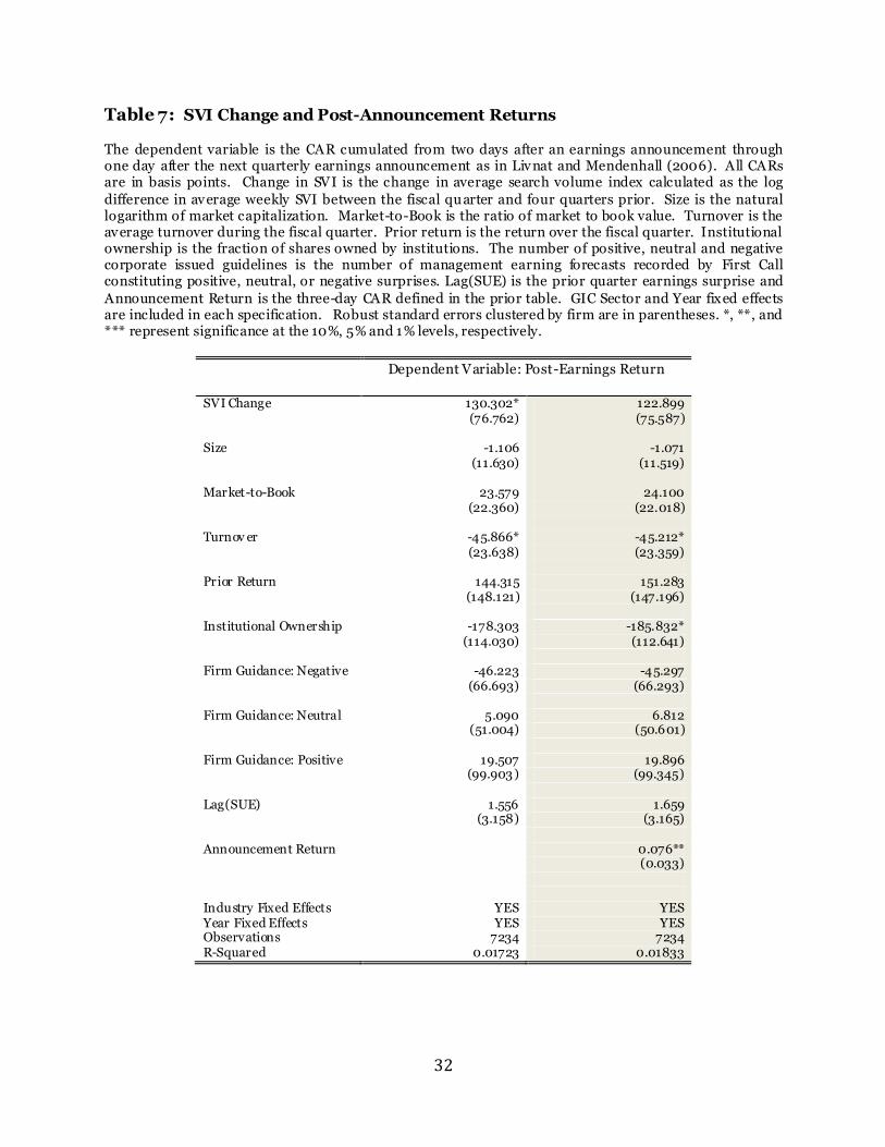
Table 7: SVI Change and Post-Announcement Returns

The dependent variable is the CAR cumulated from two days after an earnings announcement through one day after the next quarterly earnings announcement as in Livnat and Mendenhall (2006). All CARs are in basis points. Change in SVI is the change in average search volume index calculated as the log

difference in average weekly SVI between the fiscal quarter and four quarters prior. Size is the natural logarithm of market capitalization. Market-to-Book is the ratio of market to book value. Turnover is the average turnover during the fiscal quarter. Prior return is the return over the fiscal quarter. Institutional ownership is the fraction of shares owned by institutions. The number of positive, neutral and negative corporate issued guidelines is the number of management earning forecasts recorded by First Call constituting positive, neutral, or negative surprises. Lag(SUE) is the prior quarter earnings surprise and

Announcement Return is the three-day CAR defined in the prior table. GIC Sector and Year fixed effects are included in each specification. Robust standard errors clustered by firm are in parentheses. *, **, and *** represent significance at the 10%, 5% and 1% levels, respectively.

Dependent Variable: Post-Earnings Return

SVI Change 130.302* 122.899

(76.762) (75.587)

Size -1.106 -1.071

(11.630) (11.519)

Market-to-Book 23.579 24.100

(22.360) (22.018)

Turnov er -45.866* -45.212*

(23.638) (23.359)

Prior Return 144.315 151.283

(148.121) (147.196)

Institutional Ownership -178.303 -185.832*

(114.030) (112.641)

Firm Guidance: Negative -46.223 -45.297

(66.693) (66.293)

Firm Guidance: Neutral 5.090 6.812

(51.004) (50.601)

Firm Guidance: Positive 19.507 19.896

(99.903) (99.345)

Lag(SUE) 1.556 1.659

(3.158) (3.165)

Announcement Return 0.076**

(0.033)

Industry Fixed Effects YES YES Year Fixed Effects YES YES Observations 7234 7234 R-Squared 0.01723 0.01833