In or Out: Does It Matter? An Evidence-Based Analysis of ...
124
In or Out: Does It Matter? An Evidence-Based Analysis of the Euro's Trade Effects
Transcript of In or Out: Does It Matter? An Evidence-Based Analysis of ...
In or Out: Does It Matter?An Evidence-Based Analysis of theEuro's Trade Effects
Centre for Economic Policy Research (CEPR)
Centre for Economic Policy Research90-98 Goswell RoadLondon EC1V 7RRUK
Tel: +44 (0)20 7878 2900Fax: +44 (0)20 7878 2999Email: [email protected]: www.cepr.org
© Centre for Economic Policy Research 2006
British Library Cataloguing in Publication DataA catalogue record for this book is available from the British Library
ISBN: 1 898128 91 X

In or Out: Does It Matter?An Evidence-Based Analysis of theEuro's Trade EffectsRichard Baldwin, Graduate Institute of International Studies, Geneva and CEPR
This report has been financed by the Economic and Social Research Council (ESRC)through the EvidenceNetwork project. The views expressed do not represent those ofthe ESRC, CEPR or any of the other funding organisations mentioned but of theauthor alone.

Centre for Economic Policy Research (CEPR)
The Centre for Economic Policy Research is a network of over 600 Research Fellows andAffiliates, based primarily in European universities. The Centre coordinates the research activi-ties of its Fellows and Affiliates and communicates the results to the public and private sectors.CEPR is an entrepreneur, developing research initiatives with the producers, consumers andsponsors of research. Established in 1983, CEPR is a European economics research organizationwith uniquely wide-ranging scope and activities.
CEPR is a registered educational charity. Institutional (core) finance for the Centre is providedby major grants from the Economic and Social Research Council, under which an ESRCResource Centre operates within CEPR; the Esmée Fairbairn Charitable Trust and the Bank ofEngland. The Centre is also supported by the European Central Bank, the Bank for InternationalSettlements, 22 national central banks and 45 companies. None of these organizations givesprior review to the Centres publications, nor do they necessarily endorse the views expressedtherein.
The Centre is pluralist and non-partisan, bringing economic research to bear on the analysis ofmedium- and long-run policy questions. CEPR research may include views on policy, but theExecutive Committee of the Centre does not give prior review to its publications, and theCentre takes no institutional policy positions. The opinions expressed in this report are thoseof the authors and not those of the Centre for Economic Policy Research.
Chair of the Board Guillermo de la DehesaPresident Richard PortesChief Executive Officer Stephen YeoResearch Director Mathias Dewatripont

v
About the Author
Richard Baldwin has been Professor of International Economics at the GraduateInstitute of International Studies since 1991, Policy Director of CEPR since 2006 andChairman of the Foundation Board of the World Trade Institute in Bern since 2004.He was a Managing Editor of the journal Economic Policy from 2000 to 2005 andProgramme Director of CEPR's International Trade programme from 1991 to 2001.Before coming to Geneva, he was Senior Staff Economist for the President's Councilof Economic Advisors in the Bush Administration (1990-91) and Associate Professorat Columbia University Business School, having done his PhD in economics at MITwith Paul Krugman (1986), his Masters with Alasdair Smith at LSE (1981) and firstdegree with Andre Sapir (1980). He taught the PhD trade course at MIT in 2002-03and has been a visiting professor at universities in Italy, Sweden, Germany andNorway. He has also worked as a consultant for the ECB, European Commission,OECD, the World Bank, EFTA, USAID and UNCTAD. He is the author of numerousbooks and articles, including the CEPR book Towards an Integrated Europe,published in 1994. His research interests include international trade, regionalism(most recently East Asian regionalism) and European integration.
Dedication: To my father, Robert Edward Baldwin, who taught me how to think likean economist.
Acknowledgements
I would like to thank Nadia Rocha and Virginia Di Nino for assistance with data-wrestling, theory-checking and proofreading. Virginia has downloaded literally tensof millions of data points for this book and our joint work. Nadia helped me with thereview of the Rose effect literature and the trade pricing literature; she also workedout the impact of lower market-entry costs in a three-country setting (as part of herthesis). I thank Andy Rose, Volker Nitsch, Howard Wall, Alejandro Micco, and HakanNordström for providing excellent comments and answering many questions abouttheir data and regressions. They saw early drafts of Chapters 2 and 3 and eliminatedseveral mistakes. Many researchers sent me data that I have used in the figure, tablesor regressions. The list includes Stefano Tarantola, Andy Rose, Volker Nitsch, HowardWall, Alejandro Micco, Hakan Nordström, Jan Fidrmuc, and Francesco Mongelli.Daria Taglioni has helped me enormously with checking the gravity modeleconometrics. Some of the book's elements build on my earlier articles and I wouldlike to thank my co-authors (in various combinations) of those articles: BobAnderton, Frauke Skuderlny and Daria Tagloni.
Charles Wyploz, Andre Sapir and Thierry Mayer read an early complete draft of thebook and provided extremely helpful comments and critiques. I am especially indebt-ed to Charles for some late night editing/advice on the final chapter on policy impli-cations.
An early draft of Chapter 2 and some of Chapter 3 was presented at the ECB in June2005. Jeffery Frankel and Jacques Melitz were my discussants. Their insightful com-ments produced many improvements that have been included in this book. I wouldlike to thank the ECB, especially Otto Issing and Francesco Mongelli for getting meto write that paper. The paper for the ECB conference and the Frankel and Melitzcomments were published, after a long delay, as Baldwin (2006). Special thanks areextended to Francesco Mongelli who carefully read the first complete draft of my ECBpaper and caught many typos, thinkos and omissions. Philip Lane provided manyuseful pointers for my ECB paper, especially on the endogeneity of currency unions.

Contents
vii
List of Figures viiiList of Tables ixForeword xi
Executive Summary xiii
1 Introduction 1
2 Literature Review 32.1 The Rose vine: review of the pre-Euro literature 42.2 Empirical findings on the euro area 302.3 Did the Euro affect trade pricing? 40
3 Is the Euro Area Rose Effect a Spurious Result? 473.1 Lies, damned lies and statistics: VAT fraud 473.2 The Rotterdam effect 493.3 PECS: woes with ROOs 503.4 Euro depreciation and appreciation 513.5 Delayed Single Market effects 513.6 Bottom line 53
4 What Caused the Euro Area Rose Effect? 554.1 Collection of clues 554.2 Microeconomic changes that could produce a Rose effect 63
5 Testing the New-Goods Hypothesis 755.1 First look at the data 765.2 Statistical estimates 81
6 Summary and Policy Implications 876.1 Implications for nations thinking of joining the euro area 886.2 Implications for the ECB and euro area members: not a
silver bullet 926.3 Concluding remarks 93
Appendix A: Summary of the most relevant pricing studies 95
Appendix B: GDP estimates from the regressions 100
Endnotes 101
References 105
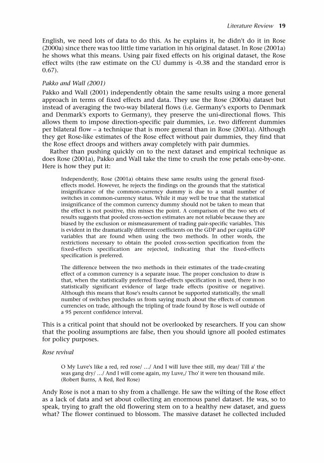
Figure 2.1 Hub and spoke common currency arrangements 5Figure 2.2 CU nations tend to be very small, poor and open 8Figure 2.3 Log averaging mistake for Germany, 2000, IMF DOTS data 12Figure 2.4 UK's share of Irish trade, 1924-98 (Thom and Walsh, 2002) 16Figure 2.5 Trade collapses in Central and Eastern Europe 18Figure 2.6 Model mis-specification and overestimation of treatment
effect 22Figure 2.7 Persson's hypothesis for why the Rose effect is overestimated 23Figure 2.8 The Rose effect over time 25Figure 2.9 Intra-euro area trade, euro area trade with others,
and trade among others, 1980-2002 32Figure 2.10 Intra- and extra-euro area trade, 1989 to 2002 32Figure 2.11 Flam-Nordström estimates of single market and euro area
dummies 38Figure 2.12 Euro against the dollar, 1999-2005 38Figure 2.13 Panel A: Difference in differences, EA and non-EA EU members,
Allington et al. (2005) 42Figure 2.14 Panel B: Difference in differences, EA and non-EA EU members,
Allington et al. (2005) 43Figure 2.15 Engel and Rogers (2004), price dispersion data by group 45Figure 2.16 Convergence and divergence of euro area inflation rates,
1990-2001 45Figure 3.1 Difference between intra-EU exports and imports 49Figure 3.2 Internal Market Index evolution euro area (EA) versus
non-euro area (non-EA) 52Figure 4.1 The euro's trade effect by nation 56Figure 4.2 The euro's trade effect over time 60Figure 4.3 Indices of European integration over time 61 Figure 4.4 Determining the number of goods in a 'new trade' model 71Figure 4.5 Determining the range of goods in a 'new new trade model 72Figure 5.1 Evolution of zeros for Germany's exports to EU15 nations,
1990-2003 77Figure 5.2 Sum of zeros for EA nations, non-EA EU nations and
non-EU nations 78Figure 5.3 Sum of zeros to EA nations from three groups of exporters
(EA, EU not EA and non-EU) 79Figure 5.4 Ratio of zeros to EA and non-EA destinations inside the EU,
'ins' versus the 'outs' 80
List of Figures
ix
List of Tables
Table 2.1 The Rose garden, currency unions considered in Rose (2000a) 7Table 2.2 Bilateral imbalance as percentage of one-way flow, US dollar
currency pairs 13Table 2.3 Rose effect estimates arranged by estimator 29Table 4.1 Trade diversion results, MSO (2003) 57Table 4.2 Internal and external trade creation, Flam and Nordström (2003)
estimates 59Table 4.3 Rose effect and volatility impact by sector 62Table 4.4 Flam-Nordström sectoral Rose effects 64Table 4.5 Transaction cost drop (%) implied by a 10% Rose effect,
various elasticities and shares 67Table 5.1 Tobit estimates: the overall Rose effect 82Table 5.2 Impact of the euro on promoting trade in new categories: logit
regressions 84Table 5.3 Impact of the euro existing trade flows, OLS regressions 86 Table 6.1 Simulation of extra imports and exports for euro area joiners 89Table 6.2 Economic size of the 'must join' nations 91Table 6.3 Simulation of extra imports and exports for likely euro area
joiners 92Table 6.4 Simulation of extra imports and exports, other new EU
members 92
CEPR hosts a node in the Economic and Social Research Council's EvidenceNetworkinitiative, which aims to advance the methodology of evidence-based policy (EBP)assessment and to apply it to a wide range of policy issues. The CEPR node is calledthe Centre for Comparative European Policy Evaluation, and its aim is to considercross-country evidence as the basis for assessing the impact of, and opportunities foreconomic policy. The Centre addresses policy issues that involve decision-making atthe EU level as well as UK policy issues for which the experiences of other Europeancountries are relevant and where comparative work across countries is likely to proveilluminating. This fourth report from the Centre, written by Professor RichardBaldwin, aims to establish a consensus estimate of the euro's impact on trade flows.
The opinions expressed herein are those of the author alone, and do not reflect theviews of the institution to which he is affiliated, the Economic and Social ResearchCouncil,or of CEPR, which takes no institutional policy positions. The Centre is,however, delighted to provide the author this forum for presentation of a subject thathas important implications for both members and non-members of the euro area.
Stephen YeoChief Executive Officer, CEPR
March 2006
xi
Foreword

Economics played little role in the decision to create the euro politics was king.Going forward, however, economics moves to centre stage. Should the euro areaworry about admitting new members who are very economically different fromincumbents? What are the costs and benefits of euro adoption for potential joiners?Are the famous Maastricht Criteria the right economic tests for potential members?How worried should the European Central Bank be about unsynchronised booms andbusts in the euro area?
The microeconomic effects of the euro are at the heart of these questions sincethey determine the extent to which euro usage will foster economic integrationamong incumbents and joiners. Two microeconomic effects are critical the impacton international capital flows, and the impact on international goods flows, i.e. trade.The focus here is on the trade flows.
This report marshals the best available empirical evidence on the size and natureof the euro's pro-trade effect. Six main findings are extracted from the empiricalresearch:
1) The pro-trade effect of the euro is modest somewhere between 5% and 15%,with 9% being the best estimate.
2) It happened very quickly, appearing in 1999.
3) It was not exclusive; euro-usage boosted imports from non-euro area nationsalmost as much as it boosted imports from euro area partners, i.e. there was notrade diversion but rather external trade creation in addition to the internaltrade creation. The best estimate of the external trade creation is 7%. The bestempirical evidence suggests that this applies only the euro area imports, butsome evidence suggests that it applies to euro area exports as well.
4) It involved little or no convergence in euro area prices despite the jump in tradeflows.
5) New research in this report suggests that reduced transaction costs were notprimarily responsible for the pro-trade effects, arguing instead that it was causedby the export of new goods to euro area economies. The mechanism driving thismay have been a reduction in the fixed cost of introducing new goods into euroarea markets. This mechanism, which is tantamount to a unilateral product-market liberalisation, would account for the lack of trade diversion (it wouldstimulate the introduction of new goods from euro area-based and non-euroarea-based exporters alike) and it would account for the jump up in tradewithout price convergence (total volumes can rise at constant prices).
6) The pro-trade effect varies a great deal across nations; Spain seems to have beenthe biggest gainer while Greece's gain is estimated to be nil or even negative.
7) The pro-trade effect varies greatly across sectors, with the gains concentrated inincreasing-returns-to-scale sectors such as machinery & transport equipment,and chemicals. Beverages & tobacco was the biggest gainer, but this may be dueto spurious factors (VAT fraud).
Executive Summary
xiii
The policy implications of these findings are grouped into two broad categories les-sons for potential joiners and lessons for the euro area's 12 members and its economicmanagement.
Why trade effects matter for potential joiners
The costs and benefits of joining the euro area are easy, according to traditional think-ing (i.e. 'optimal currency area' reasoning). The costs are on the macroeconomic side.By embracing the ECB's one-size-fits-all policy, the joiner foregoes a monetary policytailored to its national stabilisation needs. The benefits are on the microeconomicside. Adopting the euro area's currency means tighter economic integration with abloc that constitutes one-sixth of world output and 30% of world trade. But howmuch will the common currency boost trade if you do join? How much 'trade diver-sion' will you suffer if you don't join?
The potential joiners fall into two groups the medium to small sized economies(Britain, Sweden, Poland, Denmark, Czech Republic and Hungary), and the minus-cule economies (Slovenia, Slovakia, Estonia, Latvia, Lithuania, Cyprus and Malta).
A weaker economic case for joining the euro: Britain, Sweden andDenmark
The small overall size of the pro-trade effect and the lack of trade diversion weakenboth the economic case and the political economy case for British, Swedish andDanish membership in the euro area. Here is the argument.
The traditional 'optimal currency area' framework is relevant for medium and smalleconomies, especially Britain, Sweden and Denmark. Their economic-managementinstitutions can run effective monetary policies and their economies are large enoughto warrant nationally-tailored monetary policies, at least on occasion, so joiningentails a macroeconomic cost. This should be balanced by a microeconomic gain. TheUK Treasury's 2003 study on Britain's readiness to join, for example, suggests that themicroeconomic gains from using the euro may be large due mainly to a large pro-trade effect (assumed to be over 40%). This large number was based on empiricalresearch that has subsequently been discredited, as this report argues at length(Chapter 2). If the real pro-trade effect is just 9% the microeconomic gains will bemodest. Moreover, since the euro has produced 'external trade creation' much of thetrade gain the extra exports to euro area nations has already occurred and the gainto Britain, Sweden and Denmark from adopting the euro are correspondingly reduced(on exports, joiners only get the difference between the internal and external tradecreation effects, not the full 9%). In short, the lack of trade diversion means that theeconomic case for forming the euro area in the first place is quite different from thecase for joining it now.
Politics versus economics
This report's findings also suggest a sharp division between the political-economygains and the economic gains. Greater exports are a political-economy 'prize' thatshould ease the political 'sacrifice' on the stabilisation side. But the modest size of thepro-trade effect means this prize will be small. The lack of trade diversion means thatexport losses from staying out will be nil. In other words, staying outside the euroarea is not like staying out of a preferential trade area. Continuing with the political-economy mercantilist thinking, the big export winners from UK, Swedish and Danishmembership would be exporters in the euro area nations who would see their exportsto newcomers rise by 9%.
xiv In or Out: Does It Matter?
The case for joining the miniscule economies: Estonia, Latvia, Lithuania,Slovenia, Cyprus and Malta
Traditional costs-benefit analysis does not apply to many of the new members of theEU. These nations are so small that the macroeconomic cost of embracing the euro isnot a cost at all. As Andres Sutt, deputy governor of the Bank of Estonia, phrased thepoint: you can't cook a different soup in one corner of the pot. The GDPs of thesix nations most eager to join are smaller than Luxembourg's indeed, theireconomies are smaller than that of a good-sized French city. Just as issuing extra cur-rency in Dijon would do little to stimulate the local economy, pursuing an inde-pendent monetary policy in Estonia would do little good. And it could do a lot ofharm by opening the door to foreign exchange crises.
For these nations, the modest size of the euro's pro-trade effect is basically irrele-vant. The finding of external trade creation, however, implies that the costs of wait-ing are not as high as they would be if staying out entailed trade diversion. For theeuro area incumbents, however, the modest trade effects means that one cannot relyon massive increases in trade to bring these nations' economies into synch with theeuro area average. This brings us to the policy implications for the euro area's politi-cal and economic managers.
Implications for the ECB and euro area members: not a silver bullet
Although monetary union was about politics, not economics, one recent line ofthinking has cast economics in the role of facilitator. This thinking the so-called'endogenous optimal currency area' reasoning argues that monetary union producestighter economic integration within the bloc and this makes the ECB's one-size-fits-all monetary policy more appropriate for each of the euro area economies. The pro-trade effect of the euro was one of the key mechanisms suggested. It argues that thepro-trade effects helps harmonise national business cycles via, for example, 'demandspillovers' (booming demand in one nation would result in a rapid rise in importswhich would in turn stimulate output in other euro area nations).
Plainly this thinking if it were true would be very attractive to policy makers inthe euro area, the ECB and those Member States who want to join fast. To reform-weary national policy makers in the euro area, this analysis would imply that tradecreation is an easy way to harmonise the euro area economically (structural andlabour market reforms being the hard way). To potential euro-adopters, it wouldimply that they need not adjust before joining since trade creation will do the jobafter joining. To ECB monetary policy deciders, it would hold out the hope that theirjobs will get easier.
Alas, the premise is false at least as far as the trade channel is concerned. Thisthinking might have been important if the pro-trade effects were as large as the earlyliterature suggested, e.g. Rose (2000a). Chapter 2 argues that these large effects werethe product of mistaken statistical analysis and that they should be ignored for poli-cy making purposes. The best-estimate of the pro-trade effect is quite modest, so theendogenous-OCA arguments based on trade creation are of second-order importance.Of course, other channels such as financial market integration and changes in wageformation processes may still be important empirically.
Implications for prospective monetary unions in the rest of the world
The European Union is held up as an ideal of how tight economic integration pro-motes the welfare of citizens and brings peace among former enemies. To the extent
Executive Summary xv
that the logic of 'one market, one money' holds true, the path to tighter economicintegration leads inevitably to the question of a common currency. Indeed, just as thecalls for a monetary union in Europe were strengthened by the currency turbulencein Europe in the 1990s, the 1997 Asian Crisis and various Latin American currencycrises have lead to a keen interest of the economics of common currencies. The les-sons of this report for other regions of the world are that a common currency pro-vides a modest boost to trade integration, but at least for Europe, it has not been a'silver bullet.'
Caveat Emptor
With just six years of post-euro data, it is impossible to think that the empirical workreviewed and presented in this book will be the last word on the subject. Future expe-rience may revise the findings, and will certainly provide a better understanding ofthe economic mechanism through which the euro has affected trade. But one muststop somewhere. After all, books are never done, they're just due. Given the impend-ing enlargements of the euro area, this seemed a good time for stocktaking.
xvi In or Out: Does It Matter?

Just at the end of the twentieth century a century that witnessed Europeans killingEuropeans on an industrial scale something strange happened. Three hundred mil-lion Europeans abandoned their familiar francs, marks, guilders and shillings andadopted a made-up currency. They then turned over macroeconomic stabilization fora sixth of the world's economy to a made-up central bank. This was a brave step.Things turned out well economically and politically but this was not obvious before-hand. Truth be told, economists could only guess at what the economic impact wouldbe. Even now we are still working out what happened. This report's aim is to con-tribute to this ongoing 'what happened' effort.
The report focuses on the trade effects of the euro.
This may seem a narrow topic most books on the euro touch on everything frominflation psychology and supermarket pricing schemes to corporate debt markets andcentral bank governance. While narrow, the euro's trade effect is a topic that is bothcritical to policy choices and amenable to evidence-based research.
Critical to policy choicesThe euro was created for political reasons. Economics especially the trade effects was a minor issue in the minds of the men and women who launched Europe's mon-etary union. Going forward, however, economic issues play a much more central role.What are the costs and benefits of euro-adoption for potential joiners? Should theeuro area worry about letting in new members who are very economically differentto incumbents? Are the famous Maastricht Criteria, which were used in setting up theeuro area the right tests for potential members? How worried should the EuropeanCentral Bank be about unsynchronized booms and busts in the euro area?
At the heart of all these questions lie the microeconomic effects of the euro, espe-cially the extent to which the euro fosters economic integration among its members.Two effects are critical the impact of the euro on international flows of capital andcapital markets, and the impact of the euro on international flows of goods and goodsmarkets, i.e. trade. This book focuses on the latter.
Amenable to evidence-based researchFive years ago, empirical research on the trade effects of currency arrangements wascatapulted from one of the deepest cellars of academic obscurity to one of the mostactive issues in empirical international economics. The underlying cause was theemergence of vast international datasets and the empirical tools to use them, but theproximate cause was a celebrated paper by Berkeley economist Andrew Rose whichclaimed that a common currency boosted bilateral trade by 200%. Since then a broadrange of economists have marshalled a broad range of techniques and datasets to
1 Introduction
1

investigate the 'Rose effect' more thoroughly. Very recently, empirical researchershave begun to ask more pointed questions focused on the nature of the pro-tradeeffects rather than simply estimating its overall magnitude. Which sectors and whichcountries are most affected? By which economic mechanisms does a common cur-rency affect trade flows and trade pricing? This recent and rapid emergence of empir-ical work suggests that the time is ripe for a critical review and synthesis of the evi-dence-based research.
The report's organization
The first two-fifths of the report systematically sort through the existing empirical lit-erature a task that is necessary since existing estimates of a currency union's impacton trade are all over the place. Some authors claim that currency unions boost tradeby more 1000%; others find no effect or even a negative effect. To provide a structurefor evaluating the broad range of estimates, Chapter 2 also presents a theory-basedanalysis of the econometrics of the gravity model (the backbone of the empirical lit-erature) and uses this to point out many systematic errors in the literature onEuropean and non-European currency unions.
Chapter 3 considers a number of detailed data problems that may imply that theRose effect is a statistical illusion. There is no way to be absolutely sure how impor-tant these data problems are, but it is important to highlight the data limitations.
The next task is the report's heart, so to speak. Chapter 4 extracts the stylizedempirical facts from the existing literature, being careful to discard results from themany studies that are vitiated by serious econometric errors. It then goes on to do abit of Sherlock Holmes-ing. It considers a number of possible explanations and findsthat many of them are at odds with some or all of the stylized facts. The one possi-bility that seems consistent with all the facts is the 'new goods hypothesis', the notionthat the euro boosted the range of products that were exported to euro area nationsby both euro area and non-euro area nations. The economics of this sort of effect canbe tricky. Indeed, until the so-called 'new new' trade theory got started with Melitz(2003), trade economists did not have the tools to analyze carefully the logic of sucheffects.
Chapter 5 presents some de novo empirical evidence that supports the new goodshypothesis. Chapter 6 sums up the report's findings and discusses the policy implica-tions.
2 In or Out: Does It Matter?
This chapter provides a critical and synthetic review of the empirical literature on thepro-trade effects of adopting a common currency. The first section considers the pre-euro literature. The second section considers empirical studies that focus on the euro.We start, however, by putting the literature into a historical context. On the curren-cy-trade link issue economists were right, then they were wrong, and now they areright again.
A puzzling non-result
For more than a hundred years, received wisdom held that stable internationalexchange rates were essential to international trade. This belief was based largely onthe correlation between favourable trade performance and adherence to the goldstandard. As the leading gold-standard scholar Michael Bordo puts it: 'The periodfrom 1880 to 1914 is known as the classical gold standard. During that time themajority of countries adhered (in varying degrees) to gold. It was also a period ofunprecedented economic growth with relatively free trade in goods, labour, and cap-ital.'1
This received wisdom, however, was most definitely not an 'evidence-based' policyanalysis. From the time computers became widely available to economists in the1970s right up to the year 2000, economists failed to find a robust, evidence-basedlink between exchange rate volatility and trade.
This was not for want of trying.The IMF was set up in the 1940s to help fix exchange rates worldwide. When its
raison d'être the Bretton Woods fixed exchange rate system collapsed in the early1970s, IMF economists set about 'proving' that exchange rate volatility would harmworld trade. Despite a massive effort, no clear-cut evidence could be found linkingvolatility and trade flows (IMF, 1984). Some authors found the link to be negative,others positive, but most found no statistically significant link at all. When I reviewedthe literature in 1990 for a background study that I wrote for the EuropeanCommission's report One Market, One Money, active research on the topic was dead inthe water.2 The state of the art was summarized in the title of the 1991 paper byLorenzo Bini Smaghi, 'Exchange Rate Variability and International Trade: Why is it soDifficult to Find any Empirical Relationship?'3
Even with radically more sophisticated empirical techniques and an extra decadeworth of data, economists in the mid-1990s could find no link. For example, a famous1993 paper by Jeffery Frankel and Shang-Jin Wei asserted, 'if real exchange ratevolatility in Europe were to double, the volume of intra-regional trade might fall byan estimated 0.7%'.
This three-decade old failure to find empirical support for the received wisdom ledto a sort of 'cognitive dissonance' in the profession. It is summed up in the first sen-tence of an article Shang-Jin Wei published in late 1999:
3
2 Literature Review

A puzzle in empirical international finance is the difficulty in identifying a largeand negative effect of exchange rate volatility on trade. This has led to abifurcation of reactions. On the one hand, policy circles choose to ignore thisliterature, and continue to believe that exchange rate volatility has a large andnegative effect on goods trade. For example, government officials in Europeexplicitly and repeatedly cite this effect as a primary justification for the EuropeanMonetary System and the drive for a single currency in Europe. On the other hand,clever economists start to think of clever explanations for why the effect should besmall on a conceptual level.
All this was to change the year after Wei's article appeared.
2.1 The Rose vine: review of the pre-euro literature
Andy Rose of the University of California-Berkeley opened a new chapter in interna-tional economics with an Economic Policy article published in 2000. Rose (2000a)asked a simple question and got a simple answer:
What is the effect of a common currency on international trade? Answer: Large.
In fact Rose (2000a) asserted that a currency union would increase trade 200% andthis was on top of the large and negative impact he found for exchange rate volatili-ty.
Given the 25 years of futile searching described above, it is easy to understand whyRose's paper was nothing short of a revolution. Much of the response has been criti-cal, with authors trying to reduce the size of the impact. This section reviews the evi-dence on the trade effects of currency unions what I'll call the Rose effect for brevi-ty's sake on the pre-euro data. The next section reviews the evidence on the tradeeffects of the euro itself.
As an aside, I want to thank Andy for introducing a tradition of jocular writing intothis literature. The final version that Andy turned in to Charles Wyplosz (theManaging Editor of Economic Policy who did the final editing; David Begg handled themanuscript in its early stages) was chock-a-block full of exuberant English. Charlestempered some of the most avant-garde constructions, but the published version ofRose (2000a) is still a lot of fun to read. Volker Nitsch seconded this with his papersentitled: 'Honey I Shrunk the Currency Union Effect' and 'Have a Break'; I shall strug-gle to uphold the tradition in reviewing the literature.
Scientific rectitude
Andy Rose is also responsible for another remarkable feature of this literature transparency and scientific rectitude. All of Rose's datasets and regressions are postedon his website. This has permitted scholars from around the world to check his dataand results, tinker with specifications and challenge his findings. Subsequentcontributors to this literature have generally followed this stellar example.
Organization of the pre-euro literature review
This section provides a 'guided tour' of the origins, core methodologies and principalfindings of the empirical literature on pre-euro Rose effects. It is arranged inapproximate chronological order. An early version of this chapter was presented at aJune 2005 conference at the ECB; Jeffery Frankel and Jacques Melitz were mydiscussants and I thank them for the valuable comments and critiques.4
4 In or Out: Does It Matter?

2.1.1 Roots: the world through Rose coloured glasses
Rose (2000)a started the debate with his finding that countries in a currency uniontraded three times more with each other than one would expect. He arrived at thatastonishing result using a gravity-equation approach on data for bilateral tradeamong 186 nations.5 His cross-section regression was:
ln(RVod) = a0 + β1ln(RYoRYd) + β2ln(Distanceod) + β3(CUod) + controls
where RV is the real value of bilateral trade, the RYs are real GDPs of the origin nation(o is a mnemonic for origin) and destination nation (d is a mnemonic for origin), andCU is a dummy that switches on when nations o and d share a common currency. Inhis favourite regression, β3 = 1.21 which implies trade between common-currencypairs was e1.21 = 3.35 times larger than the baseline model would suggest. That meanssharing a common currency boosts trade by 235%.
The size of this common-currency effect was far too large to be believed and theprofession's assault on this claim began even before he presented it at the October1999 Economic Policy Panel that was hosted by the Bank of Finland. There were threemain themes in these critiques:
Omitted variables (omitting variables that are pro-trade and correlated with theCU dummy biases the estimate upwards).
Reverse causality (large bilateral trade flows cause a common currency ratherthan vice versa).
Model mis-specification.
Literature Review 5
Bahamas
US Virgin
Islands
Bermuda
American Samoa
Guam USA
US Virgin
Islands
Puerto Rico
Turks and CaicosIslands
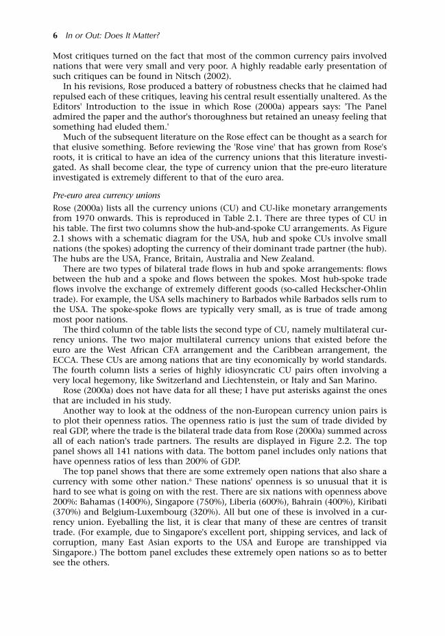
Figure 2.1 Hub and spoke common currency arrangements
Most critiques turned on the fact that most of the common currency pairs involvednations that were very small and very poor. A highly readable early presentation ofsuch critiques can be found in Nitsch (2002).
In his revisions, Rose produced a battery of robustness checks that he claimed hadrepulsed each of these critiques, leaving his central result essentially unaltered. As theEditors' Introduction to the issue in which Rose (2000a) appears says: 'The Paneladmired the paper and the author's thoroughness but retained an uneasy feeling thatsomething had eluded them.'
Much of the subsequent literature on the Rose effect can be thought as a search forthat elusive something. Before reviewing the 'Rose vine' that has grown from Rose'sroots, it is critical to have an idea of the currency unions that this literature investi-gated. As shall become clear, the type of currency union that the pre-euro literatureinvestigated is extremely different to that of the euro area.
Pre-euro area currency unions
Rose (2000a) lists all the currency unions (CU) and CU-like monetary arrangementsfrom 1970 onwards. This is reproduced in Table 2.1. There are three types of CU inhis table. The first two columns show the hub-and-spoke CU arrangements. As Figure2.1 shows with a schematic diagram for the USA, hub and spoke CUs involve smallnations (the spokes) adopting the currency of their dominant trade partner (the hub).The hubs are the USA, France, Britain, Australia and New Zealand.
There are two types of bilateral trade flows in hub and spoke arrangements: flowsbetween the hub and a spoke and flows between the spokes. Most hub-spoke tradeflows involve the exchange of extremely different goods (so-called Heckscher-Ohlintrade). For example, the USA sells machinery to Barbados while Barbados sells rum tothe USA. The spoke-spoke flows are typically very small, as is true of trade amongmost poor nations.
The third column of the table lists the second type of CU, namely multilateral cur-rency unions. The two major multilateral currency unions that existed before theeuro are the West African CFA arrangement and the Caribbean arrangement, theECCA. These CUs are among nations that are tiny economically by world standards.The fourth column lists a series of highly idiosyncratic CU pairs often involving avery local hegemony, like Switzerland and Liechtenstein, or Italy and San Marino.
Rose (2000a) does not have data for all these; I have put asterisks against the onesthat are included in his study.
Another way to look at the oddness of the non-European currency union pairs isto plot their openness ratios. The openness ratio is just the sum of trade divided byreal GDP, where the trade is the bilateral trade data from Rose (2000a) summed acrossall of each nation's trade partners. The results are displayed in Figure 2.2. The toppanel shows all 141 nations with data. The bottom panel includes only nations thathave openness ratios of less than 200% of GDP.
The top panel shows that there are some extremely open nations that also share acurrency with some other nation.6 These nations' openness is so unusual that it ishard to see what is going on with the rest. There are six nations with openness above200%: Bahamas (1400%), Singapore (750%), Liberia (600%), Bahrain (400%), Kiribati(370%) and Belgium-Luxembourg (320%). All but one of these is involved in a cur-rency union. Eyeballing the list, it is clear that many of these are centres of transittrade. (For example, due to Singapore's excellent port, shipping services, and lack ofcorruption, many East Asian exports to the USA and Europe are transhipped viaSingapore.) The bottom panel excludes these extremely open nations so as to bettersee the others.
6 In or Out: Does It Matter?
Since income is on the horizontal axis, it is easy to identify nations in the hub-and-spoke currency arrangements. Hubs are always rich and spokes are usually poor, sothe spokes are the circles to the left and the hubs are the circles to the right. The ninerich nations participating in CUs are (by declining order of GDP per capita): USA,Bermuda, Australia, Norway, France, Denmark, New Zealand, Italy and UK. Note thatRose (2000a) does not use data for all of these. For example, Bermuda, Denmark, Italyand Norway have no trade data with their CU partners so they are not included.
Given simple combinatorics, there are many, many more spoke-spoke pairs thanhub-spoke pairs (e.g. Rose (2000a) lists 16 nations using the US dollar, which implies162/2 = 128 spoke-spoke bilateral flows and 16 hub-spoke flows). Thus most of theCU pairs in the data will be between the nations with circles in the left part of thebottom panel.
Literature Review 7
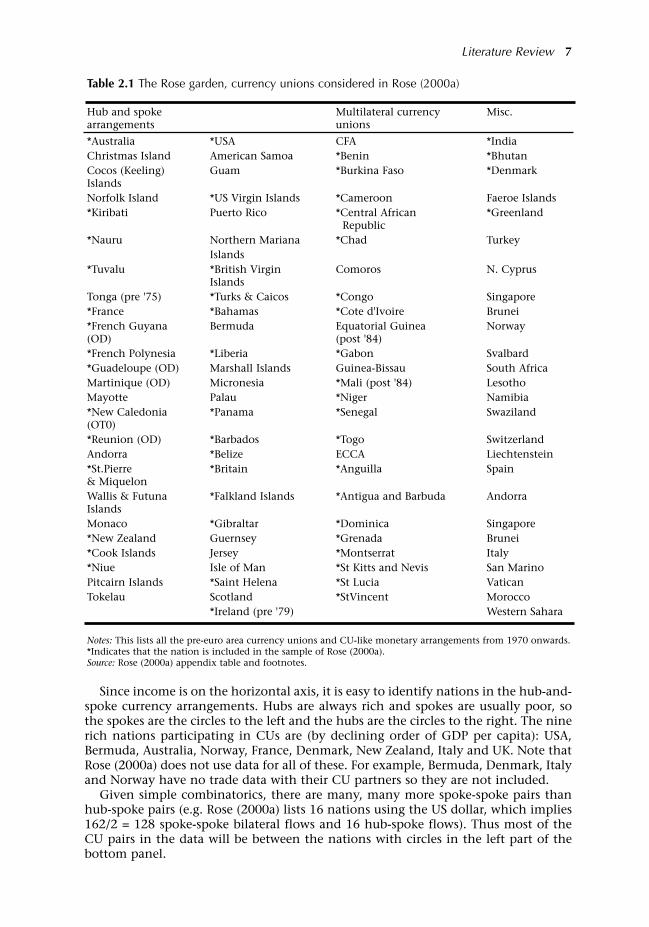
Table 2.1 The Rose garden, currency unions considered in Rose (2000a)
Hub and spoke Multilateral currency Misc.arrangements unions
*Australia *USA CFA *IndiaChristmas Island American Samoa *Benin *BhutanCocos (Keeling) Guam *Burkina Faso *DenmarkIslandsNorfolk Island *US Virgin Islands *Cameroon Faeroe Islands *Kiribati Puerto Rico *Central African *Greenland
Republic*Nauru Northern Mariana *Chad Turkey
Islands*Tuvalu *British Virgin Comoros N. Cyprus
Islands Tonga (pre '75) *Turks & Caicos *Congo Singapore*France *Bahamas *Cote d'Ivoire Brunei*French Guyana Bermuda Equatorial Guinea Norway(OD) (post '84)*French Polynesia *Liberia *Gabon Svalbard *Guadeloupe (OD) Marshall Islands Guinea-Bissau South AfricaMartinique (OD) Micronesia *Mali (post '84) LesothoMayotte Palau *Niger Namibia*New Caledonia *Panama *Senegal Swaziland(OT0)*Reunion (OD) *Barbados *Togo SwitzerlandAndorra *Belize ECCA Liechtenstein*St.Pierre *Britain *Anguilla Spain& MiquelonWallis & Futuna *Falkland Islands *Antigua and Barbuda AndorraIslandsMonaco *Gibraltar *Dominica Singapore*New Zealand Guernsey *Grenada Brunei*Cook Islands Jersey *Montserrat Italy*Niue Isle of Man *St Kitts and Nevis San MarinoPitcairn Islands *Saint Helena *St Lucia VaticanTokelau Scotland *StVincent Morocco
*Ireland (pre '79) Western Sahara
Notes: This lists all the pre-euro area currency unions and CU-like monetary arrangements from 1970 onwards.*Indicates that the nation is included in the sample of Rose (2000a).Source: Rose (2000a) appendix table and footnotes.

The main point of these graphics is that nations involved in currency unions are along way from average nations. The income levels of currency union members areeither noticeably higher than the average nation (the hubs) or considerably lowerthan the average nation (the spokes).
2.1.2 Garden pests: biases in gravity model estimations
Without theory, practice is but routine born of habit. (Louis Pasteur)
Rose (2000a) employed a naïve version of the gravity model for his preferredspecification, a version that had been widely used by policy analysts in the 1980s and
8 In or Out: Does It Matter?
Figure 2.2 CU nations tend to be very small, poor and open
Notes: Real GDP per capita on horizontal axis (US$); total trade to real GDP on vertical axis (%).Source: My calculations on the Rose (2000a) data for 1980.
0%
200%
400%
600%
800%
1000%
1200%
1400%
1600%
0 5,000 10,000 15,000 20,000 25,000 30,000 35,000 40,000
Real GDP per capita, 1980
Ope
nnes
s, (
X+
M)/G
DP
0%
20%
40%
60%
80%
100%
120%
140%
160%
180%
200%
0 2,000 4,000 6,000 8,000 10,000 12,000 14,000 16,000 18,000 20,000
Real GDP per capita
Ope
nnes
s, (
X+
M)/G
DP

1990s (including by me in my 1994 book on Eastern EU enlargement). Theinspiration for the gravity model comes from physics where the law of gravity statesthat the force of gravity between two objects is proportional to the product of themasses of the two objects divided by the square of the distance between them. Insymbols:
In trade, we replace the force of gravity with the value of bilateral trade and themasses M1 and M2 with the trade partners' GDPs (in physics G is the gravitationalconstant).
Strange as it may seem, this fits the data very well. Yet despite its goodness-of-fit,the naïve version results in severely biased results. These biases are responsible forRose's famous, and famously wrong, finding that a common currency is wildly pro-trade. To see this point we need to work through a bit of theory. Although the theo-ry does involve a small number of equations, the work is handsomely rewarded. Ithelps us understand all the mistakes in Rose (2000a) and the subsequent literature,and why only a handful of the hundreds of estimates of the Rose effect are worth pay-ing attention to for policy purposes. In any case, who ever said empirical-based poli-cy analysis should be a bed of roses?
The theory behind the gravity equation7
The gravity model is based on an expenditure equation. The value of exports of asingle good from the 'origin' nation to the 'destination' nation depends upon thegood's expenditure share and the destination nation's total expenditure on tradablegoods:
where xod is the quantity of bilateral exports of a single variety from nation o to nation'd' (o for 'origin' and d for 'destination'), pod is the price of the good inside theimporting nation measured in terms of the numeraire, so pod xod is the value of thetrade flow measured in terms of the numeraire. Also, Ed is the destination nation'sexpenditure on goods that compete with imports, i.e. tradable goods; shareod is theshare of expenditure in nation-d, one a typical variety made in nation-o.
The expenditure share depends upon relative prices and the demand elasticity. Astandard formulation for the relationship between the share and the relative price is:
where Pd is an index of the prices in nation-d of goods that compete with imports. We are interested in total exports from the origin nation to the destination nation,
so we have to multiply by the number of goods nation-o sends to nation-d to get thetotal value of bilateral exports from nation-o to nation-d. Doing this and rearranginga bit, we get:
Literature Review 9
( );
212
21
dist
MMG
gravity
offorce=
dododod Esharexp ≡
( )d
odod
elasticityodod P
ppricerelativepricerelativeshare =≡ − ,1
( ) ;1
1elasticity
d
delasticityodood
P
EpnV −
−=

where no is the number of goods nation-o exports to nation-d. If one takes nation-d'sGDP as a proxy for its expenditure on traded goods and one supposes that the priceof goods from nation-o to nation-d depends upon the distance between the twonations, this expenditure equation is very close to the gravity model. The only thingthat is missing is the GDP of the exporting nation.
The data tell us that the exporting nation's GDP should be in the gravity equation,but what is the reason? The answer involves an elementary economic fact: the export-ing nation must sell everything it produces. How much it can sell depends in turnupon the price of its goods and its market access, where market access depends uponbilateral trade costs and the geographic distribution of incomes across its trading part-ners. It is possible to work out the relationship precisely with a few lines of algebra.Doing so and plugging the result into the above expression for Vod, we have:8
where Ωo is a measure of nation-o's market access (capital omega is a mnemonic for'openness' to the origin nation's exports) and τod is a measure of the bilateral tradecosts between nation-o and nation-d.
Taking the GDP of nation-o as a proxy for its production of traded goods, andnation-d's GDP as a proxy for its expenditure on traded goods, this can be rewrittento look just like the law of gravity.
where the Ys are the nations' GDPs; I have made the temporary assumption thatbilateral trade costs depend only upon bilateral distance in order to make theeconomic gravity equation resemble the physical one as closely as possible.Importantly, G here is not a constant as it is in the physical world; it is a variable thatincludes all the bilateral trade costs between nations o and d, so it will be different forevery pair of trade partners.
Biases in Rose (2000a)
Simplifying for clarity's sake, Rose's (2000a) preferred regression is:
In words, he deflates the bilateral trade value with the United States' CPI index, anduses real GDP, namely the national GDPs deflated by a price index that converts themto US dollars and adjusts for national price differences. Rose follows a long traditionof modelling τ as depending upon natural barriers (bilateral distance, adjacency, landborder, etc), various measures of manmade trade costs (free trade agreements, etc),and cultural barriers (common language, religion, etc). His original contribution wasto add a common currency dummy to the list hard to imagine that no one hadthought of it before 2000, but that's always the case with truly brilliant research.9 Rose(2000a) estimates this on various cross-sections of his data as well as the full panel.
What is wrong with this? One big problem the gold-medal of classic gravity
10 In or Out: Does It Matter?
( ) ;1
1elasticity
d
d
o
oelasticityodod
P
EYV −
−
Ω= τ
( ) elasticitydo
elasticy PG
dist
YYG
trade
bilateral−− Ω
≡=11
12
21 11;
),(;)(1 stuffotherdistfPY
PY
PV
ododd
d
o
ood
USA
od == − ττ σ
(1)
(2)

model mistakes and one small problem the bronze-medal winner in the mistakerace. The big problem is that the omitted terms what we called the gravitationalconstant G in formula (1) are correlated with the trade-cost term, since τod enters Ωo
and Pd directly (the bilateral trade costs affect the price of traded goods in nation-dand the market access of nation-o).
Where does the bias come from? Roughly speaking, the determinants of bilateraltrade cost that are included in the regression have to do the work of the determinantsthat are left out, namely G, so the regression tells us that they are more important totrade than they really are that's elementary econometrics (omitted variable bias). Inthe case at hand, the Rose (2000a) regressions tell us that currency unions mattermuch more than they really do.
The small problem the bronze-medal mistake is the inappropriate deflation ofnominal trade values by the US aggregate price index. Rose (2000a) and other papersreviewed below offset this error by including time dummies. Since every bilateraltrade flow is divided by the same price index, a time dummy corrects the mistakendeflation procedure.10
There is another serious error in Rose (2000a) and most subsequent papers.Fortunately, this one is easier to understand.
More thorns: the silver-medal of gravity mistakes
What Rose (2000a) estimates is a bit more complex than what we showed in (2).Following standard practice, he does not work with the exports from nation-o tonation-d but rather takes the average of bilateral trade. For example, he uses theaverage of French exports to Germany and German exports to France. There isnothing intrinsically wrong with this, but since it was done without reference totheory, most researchers commit a simple, but grave error. They mistake the log of theaverage for the average of the logs. In other words, researchers first average thebilateral trade flows and then take logs in preparation for the regression; Rose (2000a)and almost all gravity equations are estimated in log-log form. In fact this mistake hasbeen repeated so many times, by so many famous economists that it has earned thecrown of respectability. It is even in one of the most common references for thegravity model (Chapter 5 in Feenstra, 2003).11
The silver-medal mistake can seriously bias the results. The sum of the logs theright way is approximately the log of the sums, but the approximation gets worseas the two flows summed become increasingly different.12 In plain English, the errorwill not be too bad for nations that have bilaterally balanced trade, but it can be trulyhorrendous for nations with very unbalanced trade. In fact, unbalanced trade is ahuge issue. The biggest exporters, German, Japan and the USA, for example, sellsomething to most nations around the world. However, many small nations sellnothing in return, at least not to all of the big-3. Thus the problem is systematicallyworse for North-South trade than it is for North-North trade.
To see the sorts of bias this mistake can induce, look at what the mistake does toGermany's bilateral trade data (IMF DOTS data for the year 2000). For nations withwhich Germany has perfect bilateral trade balance, the log of the sums is exactlyequal to the sum of the logs. But when the two flows to be averaged are quite differ-ent, the approximation becomes very wrong as Figure 2.3 shows. The extreme outlierin the figure is Germany-West Bank trade. The proper measure is 1.2 in logs, while themistaken calculation yields 2.7 in logs. The key point here is that the mistaken meas-ure is extra large for unbalanced bilateral trade relations. I also calculated this forGermany's trade with EU15 and other OECD partners for which bilateral trade ismore balanced, but still I find errors in the order of 15% even for these fairly similarnations.
Literature Review 11

By the way, the error always makes the bilateral trade look bigger (Jensen'sinequality), so if trade between currency union partners is systematically unbalanced,the silver-medal mistake means that the Rose effect will be systematicallyoverestimated.
The difference between theory and practice
For the purposes of this book, the silver-medal mistake only matters if the error isespecially bad for currency unions. To look at this quickly, I calculated the bilateralimbalance for all the hub and spoke CU pairs around the US dollar. I used IMF DOTSdata for 2000, so not all of the islands in the Rose (2000a) list are present. Table 2.2shows that most of the spoke-spoke trade flows are zero and the non-zero entries allhave imbalances in the order of 100%, so the trade flow will be severely upwardbiased. The hub-spoke flows are less likely to be zero, and the trade imbalances areless severe, but in most cases they are over 50% and so also severely overestimateddue to the silver medal mistake. Indeed, only one of the ten non-zero pairs has lessthan a 50% imbalance.
Summing up on Rose (2000)
Rose (2000a) is a great, path-breaking paper. This section has explained why thepooled estimates in Rose (2000a) the most famous of which is the +200% estimate should be ignored for policy purposes. They are based on an estimation techniquethat has subsequently been proved to be wrong by several authors, including AndyRose himself as we shall see below. Rose (2000a) is a landmark to academics, but itshould be ignored by policy makers.
Thinking of the Rose effect literature as a climbing rose springing from the Rose(2000a) roots, I turn now to the first of the three main branches of the 'Rose vine.'
12 In or Out: Does It Matter?
Figure 2.3 Log averaging mistake for Germany, 2000, IMF DOTS data
Note: The error is the incorrect (log of average) minus the correct (average of logs), for Germany's 200 or so tradepartners in the IMF DOT data for the year 2000; trade gap is the absolute value of difference in bilateral exports(to and from Germany) as percent of the smaller of the two flows. The two extreme outliers are nations withextremely unbalanced trade, West Bank/Gaza Strip and Niger. The incorrect averaging makes Germany-Nigerbilateral trade about 150% higher than it actually is when averaged correctly.
0.0
0.2
0.4
0.6
0.8
1.0
1.2
1.4
1.6
0% 2000% 4000% 6000% 8000% 10000%
Trade gap (% of smaller flow)
Erro
r

2.1.3 Rose branch #1: Rose and van Wincoop (2001)
I pass with relief from the tossing sea of Cause and Theory to the firm ground ofResult and Fact. (Winston Churchill)
Once the gold-medal mistake became clear when Jim Anderson and Eric vanWincoop published an influential paper in the American Economic Review (Andersonand van Wincoop, 2001), Andy Rose immediately teamed up with Eric van Wincoopto try to correct it. Rose and van Wincoop (2001) was the result and it shows that thegold-medal error leads to a severe upward bias in the Rose effect.
Rose and van Wincoop address the model mis-specification issue in two ways. Thesimplest is to include origin-nation and destination-nation dummies in a cross sec-tion regression. With these country dummies, the estimated Rose effect is radicallylowered; it falls by 2.7 standard deviations. However, this diminished Rose effect isstill mighty; without the country dummies a common currency is estimated to boosttrade by 3.97 times; with them by 2.48 times.
A mistaken correction of the mistake
Putting in time-invariant country-specific fixed effects is wrong, as the simple theorylaid out above shows clearly. The omitted terms in the 'gravitational constant' Greflect factors that vary every year, so the country dummies need to be time varying.If the researcher forgets about this and includes time-invariant country dummies, asRose and van Wincoop did, part of the bias may be eliminated. But since there willbe a time varying residual in the error, the results will still be biased to the extent thattrade costs are also time varying. This problem may be relatively minor in the Rose-VanWincoop data since there is very little time variation in the CU dummy (more onthis below).
This point probably explains why the second, harder way of correcting for the rel-ative-prices-matter effect in Rose-van Wincoop yields such a different result. Given allthe structure imposed on the demand system I mean the gravity equation theeconometrician can actually generate data for the omitted variables, what was calledthe 'gravitational constant' above. When they do, the estimated Rose effect is againradically reduced. Doing some rough calculations on the numbers in the paper sug-gests that the coefficient on the common currency dummy falls to 0.65, or about onemore standard deviation; with this the estimated Rose effect is 91%.
Literature Review 13
Table 2.2 Bilateral imbalance as percentage of one-way flow, US dollar currency pairs
Am. Samoa Bahamas Belize Bermuda Guam Liberia Palau Panama USA
Am. Samoa Bahamas Belize -1420% Bermuda -120% Guam Liberia 100% Palau Panama 100% 89% USA 76% 52% 91% 12% 78%
Source: My calculations on IMF DOTS for year 2000, export data.

Lessons: still a rosy scenario
What are the lessons?
(1) The estimates in the preferred regression in Rose (2000a) are just plain wrong.They are overestimated. They are overestimated because the naïve gravitymodel is mis-specified and this mis-specification matters hugely in the datasetof Rose (2000a).13
History divides neatly into two parts: pre Rose-van Wincoop and post Rose-vanWincoop. Pre-Rose-van Wincoop, we believed the 200% currency-union effectmight have been correct. Post-Rose-van Wincoop, we know better. Moregenerally, one should never pay attention to estimates of the Rose effect thatcome from the naïve gravity model, i.e. one without fixed effects à la Andersonand van Wincoop or an equivalent correction (see below).
(2) The Rose effect was still blooming after this correction; the best estimate is thatit boosts trade by 1.9 times.
(3) The omitted variable bias (stemming from G) is still in the Rose-van Wincoopnumbers, so they are still too high.
2.1.4 Rose branch #2: omitted variables
If there were such a thing as the 'Gravity model for fun and profit handbook', page 1would give this advice: 'To amaze your friends with another important trade effect,develop a new proxy for trade costs and use a really big dataset; success is notguaranteed, but you're likely to find significance (standard errors involve the inverseof the square root of number of observations) and you'll have loads of fun in anycase.' This is too cynical, but the basic point is that the gravity model omits anincredible range of factors that are likely to affect bilateral trade I've seen people getstatistically significant coefficients on time zones, language proximity, membershipin the Austro-Hungarian Empire, presence of a Chinatown in the two capitals just toname a few. More to the point, consider the trade among the nations listed in Table2.1 and ask yourself: 'Can we be sure that Rose has not left out some key trade-boosting factor that operates between many CU pairs?'
This matters for the Rose effect estimate since many of those omitted factors maybe correlated with the CU dummy. As mentioned above, this leads to an omitted vari-able bias that implies that the reported effect is too large. There are ways of address-ing this problem econometrically, and we'll get to them soon. It is useful, however, toget an idea of just what sort of omitted variables we are talking about.
Exceptions that prove the Rose14
When the editors of Economic Policy at the presentation of the original Rose paper saidthey had 'an uneasy feeling that something had eluded them', one of the many thingsthat bothered them was that they did not know enough about the particulars of theCU pairs that drove Rose's results. Maybe if one were an expert on West African trade,as one panellist suggested to me, one would have known exactly what omittedvariable explained the overestimate of the Rose effect. The literature follows up onthis in two ways. The first is to look at particular cases where we do really understandwhat was going on. The second is to play with the CU dummy. I address theseapproaches in order.
14 In or Out: Does It Matter?

A parable Imagine an economist asserted that the growth of the money supply was the maincause of long-run inflation and estimated the link using a huge international dataset.Using money supply growth and a handful of other variables that were available for150 nations, he or she estimates that the money-price elasticity is unity and everyother explanatory variable has a negligible effect on inflation. Then suppose anothereconomist showed that Ireland's money supply grew at 300% for decades but itsinflation rate was zero. This would make one pause. It would make one think thatmaybe something else is going on. The point is that counterexamples matter inempirical work; the counter-example investigator can consider a much more subtlemodel of the phenomenon since much more information is available than in the caseof 150-nation sample.
I think the counter-example approach is especially important for the Rose effect.The sorts of variables that are available for 150 nations are the sorts of variables thatmatter for average nations. But Rose looked at a phenomenon that was limited to dis-tinctly non-average nations. Thus, maybe using the 150 nation dataset approachguarantees that no one can find the 'silver bullet' pro-trade variable that would makethe Rose effect disappear because no one bothered to gather internationally compa-rable information on a factor that matters only for a couple of dozen very unusualnations. This is why I think the counter examples considered below must be takenvery seriously.
Revolutions, economic chaos and asymmetric inflation lead to CU dissolutionMany currency union break ups are done in the context of, or as the result of massivesocial, economic and/or political turmoil, many in the context of revolutions. AsThom and Walsh (2002) write:
Many of these unions ended as part of a bloody decolonizing process followed bythe adoption of Marxist/autarkic policies, bilateral trade deals with the SovietUnion or China, and a descent into economic chaos France and Algeria, whoseindependence was granted only after a bitter struggle; India and Pakistan, whoended their currency union after the war of 1965; Pakistan and Bangladesh, whosplit up after the war of 1971; South Africa and Southern Rhodesia (Zimbabwe)who were ejected from the Commonwealth and had trade sanctions imposed asthey broke with sterling; the five Portuguese colonies in Africa, that broke withPortugal after wars of liberation followed by civil wars. In all these cases and manyothers it is very likely that trade between the former currency union partnerswould have collapsed regardless of the currency regime in force.
If this is right, the silver-bullet is the mysterious third cause that drove the revolution,currency union break up and decline in trade. The same is true for currency unionjoiners. The decision to adopt a currency for example, to dollarize takes place inthe context of great political and economic changes, many of which could beexpected to affect trade. Plainly no one has good data on such factors oh sure thereare proxies to be found in hyperspace but such things really cannot be accuratelymeasured with a one-dimensional variable; if they could, we wouldn't need historiansand political scientists. Be that as it may, my point is that one cannot see whether theRose effect survives the inclusion of this sort of mysterious third effect in the Rose,Rose-Wincoop or Glick-Rose datasets. We also need case studies.
Thom and Walsh (2002): the bloom on 'my wild Irish rose' is not for the takingIreland used the British pound before its independence. After independence and theintroduction of the Irish pound in 1927, the pound-punt exchange rate was held at1-to-1 with no margins. Talks leading up the European Monetary System suggested
Literature Review 15

that this peg would remain in the context of the ERM since everyone initiallyexpected Britain to join. When Thatcher said no in 1979, Ireland was forced to choosebetween 'Europe' (as they call it in Britain) and the ERM on one hand, and Britain andsterling on the other. Ireland chose Europe and the 1-to-1 peg was abandoned. Marketforces lifted the rate rapidly away from the level it had been at for 50 years. Whathappened to Anglo-Irish trade?
Since Ireland and the UK were both embedded in the EEC, the termination of thecurrency union did not and could not raise bilateral trade barriers. Moreover, bothnations were run by stable, predictable governments and although there certainlywere a number of idiosyncratic factors affecting bilateral trade, one has a very goodidea of what they were and very good data that allows one to control for them. Inshort, we should be able to learn a lot about the Rose effect by studying the Irish case.One recent investigation of this example, Thom and Walsh (2002), finds no evidencefrom time series or panel regressions that the change of the exchange rate regime hada significant effect on Anglo-Irish trade. Should we be shocked?
Let's set out the priors. If the Rose effect discussed in Rose (2000a) is roughly right,the currency regime switch should have reduced Anglo-Irish trade to about a third ofits initial level. The impact on Ireland should have been massive since the UKabsorbed about half Ireland's exports at the time. Even if there were countervailingforces generated by the break up, it is hard to imagine any such forces that would all else equal raise Anglo-Irish trade by enough to substantially offset a Rose effectof -200%. By contrast, if the lower ranges of the Rose effect are right say the effectis 15% then we might miss the Rose effect in the Irish experience especially if onethinks the 15% would take a number of years to be realized. My point here is that theIrish experience might help us reject a big Rose effect, but not a modest one.
Inspection of Figure 2.4 shows that the initial Rose effect just could not have beenright. OK, one should run some regressions and talk about the standard errors (Thomand Walsh do), but really, would you ever believe a regression that says the data in
16 In or Out: Does It Matter?
Figure 2.4 UK's share of Irish trade, 1924-98
19241929
19341939
19441949
19541959
19641969
19741979
19841989
1994
10
20
30
40
50
60
70
80
90
100
%
Source: (Thom and Walsh, 2002)

this figure were generated by a model where trade would have dropped by 200% in1979 were it not for some offsetting effect?15
I think there are other lessons in Figure 2.4. The gradual decline of Anglo-Irish trade was due to structural changes, in my opin-
ion mainly changes in the Irish economy. As Ireland developed from a potato-exporting agrarian economy into the Celtic Tiger it is today, its trade pattern natu-rally eroded from its historical overdependence on its nearest market (the UK). Thissort of thing is not in any version of the gravity model. The closest would be to allowfor a separate GDP per capita variable for exporter and importer nations (for theexporter it would reflect structural shifts, for the importer an income elasticity), butRose only includes the product of the two. Now suppose one threw into the gravityequation the 1965 Anglo-UK free trade agreement, the 1974 adhesion to the EEC anda CU dummy. Moreover, suppose one did this in a panel where it is not really possi-ble to check for serial correlation in the errors. Plainly, the CU dummy would pick upmost of the action of the omitted variables that explained Ireland's historic overdependency on the British economy. One could throw in proxies for colonial rela-tions in various guises, but none of this would pick up the structural transformationof the Irish economy. Moreover, the history related by Thom and Walsh makes it clearthat the reduced dependency on the British market which was driven by factors thatare unobservable to the gravity model is one of the factors that caused the CurrencyUnion to break up (more on reverse causality below).
Fidrmuc and Fidrmuc (2003): Central and Eastern European break-upsThe eyeball evidence for a large Rose effect looks much better for the recent break-upsof currency unions in Central and Eastern Europe. Figure 2.5, taken from Fidrmuc andFidrmuc (2003), shows that the break-ups were followed by dramatic drops inbilateral trade.
The top left panel makes that best case for a large, negative Rose effect due to a cur-rency union break-up. In 1993, Czechoslovakia went through a 'velvet divorce' just afew years after its 'velvet revolution'. The two parts of the nation separated into theCzech Republic and the Slovak Republic. They maintained a customs union (no tar-iffs between them and a common external tariff) until they simultaneously joined theEU's customs union. On the face of it, this is just the sort of natural experiment oneshould study. Figure 2.5 plots year-by-year estimates of the above normal level oftrade between the partners (this is the exponent of the pair dummy, e.g. the Czechand Slovak dummy in the Czechoslovak case). But even here one must raise a note ofcaution. As Fidrmuc and Fidrmuc's paper concludes:
Our findings are broadly consistent with earlier findings on currency unions. Inparticular, Rose (2000a) shows that a common currency increases bilateral trade flowsapproximately three times. Indeed, we found a decline of bilateral trade intensity byabout this factor during the first years of independence. However, we cannot separatethe effect of the currency separation from that of the political disintegration as botheffects occurred (more or less) simultaneously in the countries under scrutiny.
The total drop was less than the size of Rose's first estimate of 200%, with the sizeof the pair dummy falling 100% from about 4.0 to about 2.0. At one extreme, wecould claim that the only thing affecting this trade was the loss of a common cur-rency. This is rather naïve, but it gives a Rose effect of 2.0, which is similar to manyestimates. Yet one suspects that political and economic disintegration also loweredtrade. This means that a 100% currency union trade effect is too high; the Rose effectin isolation would be smaller. To explore this conjecture, it would be interesting torevisit the Fidrmuc-Fidrmuc data using some of the more sophisticated methods dis-cussed above to sort out the two effects.
Literature Review 17

Further observations follow from this work. Fidrmuc and Fidrmuc provide aqualitative discussion of the changes that accompanied the currency uniondissolutions. Their discussion makes it clear that many time-varying, pair-specificomitted variables that affect trade were spawned by the same forces that lead to theCU break-up. To list just one of a dozen stories, the Czechs and Slovaks maintainedfree trade after the currency split, but they set up border controls that some businessesclaimed acted as a trade barrier. None of these stories could be included in regressionslike Rose estimates since there would be no way to gather such data for 100+ nations. The lessons from these two cases are unclear in terms of specifics, but crystal clear interms of generalities lots of other complicated stuff matters. And it is the sort offactors on which we will never have good, internationally comparable data. In short,gravity equations will always have omitted variables.
A recent paper takes issue with the Fidrmuc-Fidrmuc paper when it comes to theformer Yugoslavia. Using more complete data than Fidrmuc and Fidrmuc (2003), DeSouza and Lamotte (2006) find that the drop in trade was not dramatic but rathersmooth.
Pair dummies: Glicks 'N Roses
Andy Rose was, of course, well aware of the omitted variable bias critique even beforeit was echoed many times by Economic Policy referees and panellists in Helsinki. Hewas also well aware that using pair-specific dummies would wipe out all idiosyncraticlevel effects between all pairs of nations. The only sticking point is that this tends tothrow the roses out with the vase water. It eliminates all cross-section variation fromthe residual, so the identification comes solely from time series variation.16 In plain
18 In or Out: Does It Matter?
Figure 2.5 Trade collapses in Central and Eastern Europe
1991 1992 1993 1994 1995 1996 1997 1998 1990 N/A 1992 1993 1994 1995 1996 1997 1998
1992 1993 1994 1995 1996 1997 1998 1992 1993 1994 1995 1996 1997 1998
4.00
3.50
3.00
2.50
2.00
1.50
1.00
0.50
0.00
4.50
4.00
3.50
3.00
2.50
2.00
1.50
4.50
4.00
3.50
3.00
2.50
2.00
1.50
4.50
4.00
3.50
3.00
2.50
2.00
1.50
Source: Fidrmuc & Fidrmuc (2003).
Former Czechoslovakia Slovenia-Croatia
Russia-Ukraine-Belarus Baltic States
English, we need lots of data to do this. As he explains it, he didn't do it in Rose(2000a) since there was too little time variation in his original dataset. In Rose (2001a)he shows what this means. Using pair fixed effects on his original dataset, the Roseeffect wilts (the raw estimate on the CU dummy is -0.38 and the standard error is0.67).
Pakko and Wall (2001)
Pakko and Wall (2001) independently obtain the same results using a more generalapproach in terms of fixed effects and data. They use the Rose (2000a) dataset butinstead of averaging the two-way bilateral flows (i.e. Germany's exports to Denmarkand Denmark's exports to Germany), they preserve the uni-directional flows. Thisallows them to impose direction-specific pair dummies, i.e. two different dummiesper bilateral flow a technique that is more general than in Rose (2001a). Althoughthey get Rose-like estimates of the Rose effect without pair dummies, they find thatthe Rose effect droops and withers away completely with pair dummies.
Rather than pushing quickly on to the next dataset and empirical technique asdoes Rose (2001a), Pakko and Wall take the time to crush the rose petals one-by-one.Here is how they put it:
Independently, Rose (2001a) obtains these same results using the general fixed-effects model. However, he rejects the findings on the grounds that the statisticalinsignificance of the common-currency dummy is due to a small number ofswitches in common-currency status. While it may well be true that the statisticalinsignificance of the common currency dummy should not be taken to mean thatthe effect is not positive, this misses the point. A comparison of the two sets ofresults suggests that pooled cross-section estimates are not reliable because they arebiased by the exclusion or mismeasurement of trading pair-specific variables. Thisis evident in the dramatically different coefficients on the GDP and per capita GDPvariables that are found when using the two methods. In other words, therestrictions necessary to obtain the pooled cross-section specification from thefixed-effects specification are rejected, indicating that the fixed-effectsspecification is preferred.
The difference between the two methods in their estimates of the trade-creatingeffect of a common currency is a separate issue. The proper conclusion to draw isthat, when the statistically preferred fixed-effects specification is used, there is nostatistically significant evidence of large trade effects (positive or negative).Although this means that Rose's results cannot be supported statistically, the smallnumber of switches precludes us from saying much about the effects of commoncurrencies on trade, although the tripling of trade found by Rose is well outside ofa 95 percent confidence interval.
This is a critical point that should not be overlooked by researchers. If you can showthat the pooling assumptions are false, then you should ignore all pooled estimatesfor policy purposes.
Rose revival
O My Luve's like a red, red rose/ / And I will luve thee still, my dear/ Till a' theseas gang dry/ / And I will come again, my Luve,/ Tho' it were ten thousand mile.(Robert Burns, A Red, Red Rose)
Andy Rose is not a man to shy from a challenge. He saw the wilting of the Rose effectas a lack of data and set about collecting an enormous panel dataset. He was, so tospeak, trying to graft the old flowering stem on to a healthy new dataset, and guesswhat? The flower continued to blossom. The massive dataset he collected included
Literature Review 19

annual data from 1948 to 1997 on bilateral trade between 217 countries.Theoretically, that's 50(2172)/2 = 2,354,450 data points, but with missingobservations and zero flows (lots of little nations sell nothing to each other), the newRose dataset has 219,558 observations.
Glick and Rose (2002) exploit this data in a number of ways. They throw in pair-specific dummies that soak up any sort of idiosyncratic omitted variables that do notvary between 1948 and 1997. This, of course, mimics the impact of country-dummiesas in Rose-van Wincoop, but it goes further. The result was, as we should have expect-ed in the post-Rose-van Wincoop world, that the size coefficient drops dramatically about 5 standard deviations from an estimated coefficient of 1.3 to 0.65. This bringsdown the Rose effect from 3.7 to 1.9 times more trade among CU pairs (both esti-mates are statistically significant at any conceivable level of confidence).
What is going on here? The estimates are still biasedPretend, for a moment, that Glick and Rose did their regression in two stages. First,they regressed the left-hand side variable on the time-invariant pair dummies.Second, they regressed the residuals from that regression on the main right-hand sidevariables, distance, CU and the joint real GDP variable. This procedure is terriblyinefficient in the econometric and practical sense, but it is very efficient from anintuitive stand point.
The first stage strips out all time-invariant features of each bilateral trade flow. Thiscompletely removes the bias stemming from the cross-section correlation betweenthe currency union (CU) dummy and various omitted determinants of bilateral tradecosts. It does the same for the cross-section correlation between what we called thegravitational constant term G and the CU dummy. However, there is almost surely abias left. We know that the relative-prices-matter term varies over time, so there willstill be a correlation with CU, after all the theory tells us that the G term contains CUand CU itself is time varying.
Second, there may still be a bias stemming from time-series correlation with omit-ted variables. For example, if currency union encourages nations to deepen otherforms of integration that are unobservable to the econometrician, then CU and theunobserved variables could be correlated over time as well as in a cross-section sense.This is especially true since each pair gets only one dummy for the full 1948-97 dataperiod.
Stop and smell the rosesWhat do we learn from this? First, the impact of allowing for country-specificidiosyncrasies (either via the Rose-Wincoop partner-dummy procedure or by theGlick-Rose technique of pair dummies) reduces the Rose effect massively. Thisconfirms yet again that the original +200% Rose effect was overestimated. Of course,90% more trade is still a huge number, but 200% is huger.
Second, the Glick-Rose result should have a large 'caveat emptor' stamped across itsforehead. The pair dummies mean that all the identification is coming from the wayin which trade between CU pairs changes over the sample, compared to the way itchanges for the non-CU pairs, controlling for other factors. The Glick-Rose data havelots of pairs that leave monetary or currency unions, but very few that join (16 join-ers and 130 leavers, with almost all of them having happened before the post-warindependence wave ended around 1970). This means that the results are being driv-en by how much trade dropped after a nation leaves a monetary union, not by howmuch trade is created by a currency union. Nitsch (2002) estimates these effects ofcurrency union joiners separately and finds the point estimate is small (about +8%)and statistically indistinguishable from zero.
20 In or Out: Does It Matter?

To put it differently, if you want to know how much a small nation's trade mightdrop if something happens such that it has to, or wants to, leave its currency union,then the Glick-Rose numbers are what you need. If you want to know how muchtrade a small nation would gain from abandoning its own currency and adoptingsomeone else's, the Glick-Rose numbers are not what you need. I think we have toadmit that there just haven't been enough new currency unions to answer the ques-tion. Or at least not until the euro area came along, but I'm saving that part of thestory for later.
Why are the country and pair dummy results so similar?Third, the point estimates from the Rose-Wincoop and Glick-Rose approaches areamazingly similar. With the naïve gravity model the Rose effect is 3.97 in the Rose-Wincoop dataset; it is 3.66 in the Glick-Rose dataset. Allowing country-specificidiosyncrasies drops the estimate to 1.9 times more trade among CU pairs in bothdatasets.
This, I believe, is reassuring on the one hand, but worrying on the other. The reas-surance is obvious; different datasets, same results. The worry is that it seems to makeno difference whether one controls only for country-specific idiosyncrasies or onecontrols for country-specific idiosyncrasies and all other pair-specific idiosyncrasies.Why worry?
My priors are that there are omitted variables correlated with the CU dummy e.g.the quality of FTAs, informal ethnic networks, foreign direct investment flows (tradeand FDI are complements empirically), and many more for which the data is non-existent or too poor to use in a regression. If my priors are right, the pair dummiesare not doing their job properly. The why-part is easy.
Many of the pair-specific omitted variables probably varied over the five decadesin the Glick-Rose dataset. Thus, putting in a time-invariant pair dummy leaves a time-series trace in the residual and this trace is probably still correlated with the CUdummy. In particular, there are probably pair-specific factors that caused nations toleave currency unions and these are probably time-varying. This is certainly the les-son to draw from the case studies. More rigorously, Nitsch (2002) uses a large panelof currency union pairs to identify factors involved in the break-up. Inter alia, hefinds that departures from currency unions tend to occur when there are large infla-tion differences among member countries, and when there is a change in the politi-cal status of a member.17
Glick and Rose try out an admirable range of robustness checks, but they obviatemost of the merit of the exercise by trying them one by one. For example, they usedata from tiny nations in 1950 in the same regression as data from the United Statesin 1995. It would take a brave soul to assert that the income elasticity of imports wasthe same number in these two cases. Tenreyro (2001) is particularly strong on thisidea that one must address all the problems together. Sure, that's a lot of regressionsto try, but you have to water the thorn to harvest the rose.
2.1.5 Rose branch #3: complicated mis-specification
There are two ways of correcting for omitted variable biases. The Glick-Rose approachworks by throwing lots of dummies into the regression. The alternative works bythrowing lots of observations out of the regression. That sounds strange, but it hasmany merits. Torsten Persson's 2001 paper in Economic Policy introduced thistechnique into the Rose effect literature. The technique is subtle and complex;Persson explains it in technical terms (and you should have seen how technical it wasbefore Giuseppe Bertola rewrote it in his role as Managing Editor of Persson's paper).18
Literature Review 21
Allow me to relate a parable that may make the nature and intractability of theproblem clearer.
A parable
A few years ago, middle-age surprised a 'friend of mine' and it chose to focus on hismiddle; he developed a little belly. He decided to do something about it and, beingan egghead, he started reading studies on the effectiveness of dieting. One studyfound that a week's worth of dieting was astoundingly effective. I have plotted thedata in Figure 2.6 (at least the data as my friend remembers it). Crucial background:People tend to gain weight as they get older (their metabolism slows), so there is anempirical link between weight and gaining weight. A proper account of theeffectiveness of dieting must take account of this. Assuming the link is linear, thestudy fitted the curve shown with the dashed line. However, medical science (as myfriend remembers it) tells us that the true weight-to-weight-gain link is bell shaped.(Once you reach middle age you pile on an extra 10 kilos and this rapidly pushes youjust beyond the normal body mass index, or BMI, range but then the process slowsdown.)
With this background we can see how the study overestimated the dieting effect.The solid dots are the weight gain of dieters and you can plainly see that they arebelow the linear dashed line. The study claimed therefore that dieting was very effec-tive, controlling for other factors. Obviously, this is a spurious finding since thedieters' weight gain is white noise around the true-model prediction without dieting.Why the incorrect inference? The subtle interaction between nonlinearity and self-selection.First, if the study had estimated the correct nonlinear model, it would have foundthat dieting was useless. Second, if the true relationship had been linear, then thededuction would have been valid. Finally, if dieting were randomly distributed acrossall weight classes, the model mis-specification would not have mattered since therewould have been an equal number of dieters above and below the fitted line (that'swhat OLS does). But, dieting is self-selected. The people who are most likely to starta diet are ones, like my friend, who have just crossed into the 'jolly but not yet jelly'category.
With this parable in hand, we turn to Persson's critique.
22 In or Out: Does It Matter?
True model without dieting
BMI
Kilos lost during weeklong diet
Normal range
0
Fitted assuming linear model
True model without dieting
BMI
Kilos lost during weeklong diet
Normal range
0
Fitted assuming linear model
Figure 2.6 Model mis-specification and overestimation of treatment effect
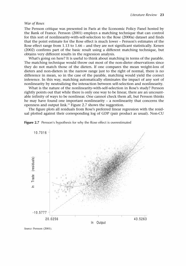
War of Roses
The Persson critique was presented in Paris at the Economic Policy Panel hosted bythe Bank of France. Persson (2001) employs a matching technique that can controlfor this sort of nonlinearity-with-self-selection to the Rose (2000a) dataset and findsthat the point estimate for the Rose effect is much lower Persson's estimates of theRose effect range from 1.13 to 1.66 and they are not significant statistically. Kenen(2002) confirms part of the basic result using a different matching technique, butobtains very different results in the regression analysis.
What's going on here? It is useful to think about matching in terms of the parable.The matching technique would throw out most of the non-dieter observations sincethey do not match those of the dieters. If one compares the mean weight-loss ofdieters and non-dieters in the narrow range just to the right of normal, there is nodifference in mean, so in the case of the parable, matching would yield the correctinference. In this way, matching automatically eliminates the impact of any sort ofnonlinearity by neutralizing the interaction between self-selection and nonlinearity.
What is the nature of the nonlinearity-with-self-selection in Rose's study? Perssonrightly points out that while there is only one way to be linear, there are an uncount-able infinity of ways to be nonlinear. One cannot check them all, but Persson thinkshe may have found one important nonlinearity a nonlinearity that concerns theopenness and output link.19 Figure 2.7 shows the suggestion.
The figure plots all residuals from Rose's preferred linear regression with the resid-ual plotted against their corresponding log of GDP (pair product as usual). Non-CU
Literature Review 23
ln
Trad
e (re
sidu
als)
ln Output2 0 . 0 2 5 6 4 3 . 5 2 6 3
- 1 0 . 5 7 7 7
1 0 . 7 0 1 6
Figure 2.7 Persson's hypothesis for why the Rose effect is overestimated
Source: Persson (2001).
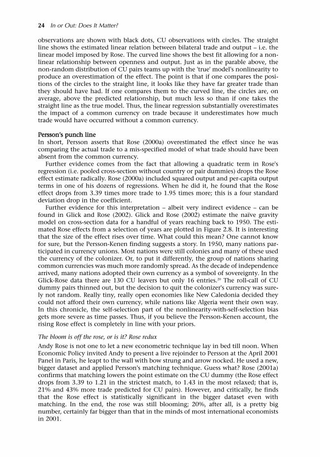
observations are shown with black dots, CU observations with circles. The straightline shows the estimated linear relation between bilateral trade and output i.e. thelinear model imposed by Rose. The curved line shows the best fit allowing for a non-linear relationship between openness and output. Just as in the parable above, thenon-random distribution of CU pairs teams up with the 'true' model's nonlinearity toproduce an overestimation of the effect. The point is that if one compares the posi-tions of the circles to the straight line, it looks like they have far greater trade thanthey should have had. If one compares them to the curved line, the circles are, onaverage, above the predicted relationship, but much less so than if one takes thestraight line as the true model. Thus, the linear regression substantially overestimatesthe impact of a common currency on trade because it underestimates how muchtrade would have occurred without a common currency.
Persson's punch lineIn short, Persson asserts that Rose (2000a) overestimated the effect since he wascomparing the actual trade to a mis-specified model of what trade should have beenabsent from the common currency.
Further evidence comes from the fact that allowing a quadratic term in Rose'sregression (i.e. pooled cross-section without country or pair dummies) drops the Roseeffect estimate radically. Rose (2000a) included squared output and per-capita outputterms in one of his dozens of regressions. When he did it, he found that the Roseeffect drops from 3.39 times more trade to 1.95 times more; this is a four standarddeviation drop in the coefficient.
Further evidence for this interpretation albeit very indirect evidence can befound in Glick and Rose (2002). Glick and Rose (2002) estimate the naïve gravitymodel on cross-section data for a handful of years reaching back to 1950. The esti-mated Rose effects from a selection of years are plotted in Figure 2.8. It is interestingthat the size of the effect rises over time. What could this mean? One cannot knowfor sure, but the Persson-Kenen finding suggests a story. In 1950, many nations par-ticipated in currency unions. Most nations were still colonies and many of these usedthe currency of the colonizer. Or, to put it differently, the group of nations sharingcommon currencies was much more randomly spread. As the decade of independencearrived, many nations adopted their own currency as a symbol of sovereignty. In theGlick-Rose data there are 130 CU leavers but only 16 entries.20 The roll-call of CUdummy pairs thinned out, but the decision to quit the colonizer's currency was sure-ly not random. Really tiny, really open economies like New Caledonia decided theycould not afford their own currency, while nations like Algeria went their own way.In this chronicle, the self-selection part of the nonlinearity-with-self-selection biasgets more severe as time passes. Thus, if you believe the Persson-Kenen account, therising Rose effect is completely in line with your priors.
The bloom is off the rose, or is it? Rose redux
Andy Rose is not one to let a new econometric technique lay in bed till noon. WhenEconomic Policy invited Andy to present a live rejoinder to Persson at the April 2001Panel in Paris, he leapt to the wall with bow strung and arrow nocked. He used a new,bigger dataset and applied Persson's matching technique. Guess what? Rose (2001a)confirms that matching lowers the point estimate on the CU dummy (the Rose effectdrops from 3.39 to 1.21 in the strictest match, to 1.43 in the most relaxed; that is,21% and 43% more trade predicted for CU pairs). However, and critically, he findsthat the Rose effect is statistically significant in the bigger dataset even withmatching. In the end, the rose was still blooming; 20%, after all, is a pretty bignumber, certainly far bigger than that in the minds of most international economistsin 2001.
24 In or Out: Does It Matter?
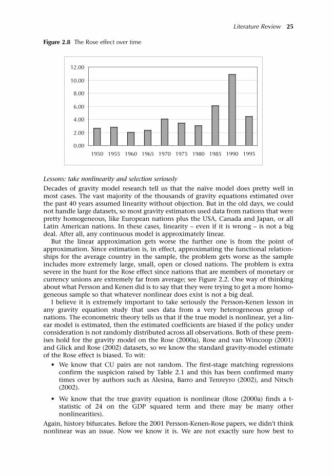
Lessons: take nonlinearity and selection seriously
Decades of gravity model research tell us that the naïve model does pretty well inmost cases. The vast majority of the thousands of gravity equations estimated overthe past 40 years assumed linearity without objection. But in the old days, we couldnot handle large datasets, so most gravity estimators used data from nations that werepretty homogeneous, like European nations plus the USA, Canada and Japan, or allLatin American nations. In these cases, linearity even if it is wrong is not a bigdeal. After all, any continuous model is approximately linear.
But the linear approximation gets worse the further one is from the point ofapproximation. Since estimation is, in effect, approximating the functional relation-ships for the average country in the sample, the problem gets worse as the sampleincludes more extremely large, small, open or closed nations. The problem is extrasevere in the hunt for the Rose effect since nations that are members of monetary orcurrency unions are extremely far from average; see Figure 2.2. One way of thinkingabout what Persson and Kenen did is to say that they were trying to get a more homo-geneous sample so that whatever nonlinear does exist is not a big deal.
I believe it is extremely important to take seriously the Persson-Kenen lesson inany gravity equation study that uses data from a very heterogeneous group ofnations. The econometric theory tells us that if the true model is nonlinear, yet a lin-ear model is estimated, then the estimated coefficients are biased if the policy underconsideration is not randomly distributed across all observations. Both of these prem-ises hold for the gravity model on the Rose (2000a), Rose and van Wincoop (2001)and Glick and Rose (2002) datasets, so we know the standard gravity-model estimateof the Rose effect is biased. To wit:
We know that CU pairs are not random. The first-stage matching regressionsconfirm the suspicion raised by Table 2.1 and this has been confirmed manytimes over by authors such as Alesina, Barro and Tenreyro (2002), and Nitsch(2002).
We know that the true gravity equation is nonlinear (Rose (2000a) finds a t-statistic of 24 on the GDP squared term and there may be many othernonlinearities).
Again, history bifurcates. Before the 2001 Persson-Kenen-Rose papers, we didn't thinknonlinear was an issue. Now we know it is. We are not exactly sure how best to
Literature Review 25
0.00
2.00
4.00
6.00
8.00
10.00
12.00
1950 1955 1960 1965 1970 1975 1980 1985 1990 1995
Figure 2.8 The Rose effect over time

address the nonlinearity, but we know it is a problem. Two more lessons:
For policy purposes, we should ignore all Rose effect estimates on large datasetsthat do not address the nonlinearity-cum-selection issue. Researchers would bewise to address it in both ways: (1) try out various nonlinearities; in the contextof Rose effect regressions, be sure to try quadratic terms for GDP and GDP percapita; (2) try matching procedures like those suggested by Persson or Kenen.
The Rose effect on multilateral data is of the order of about 20-40%, but thisfigure basically reflects the extent to which bilateral trade dropped betweennations when a currency union pair involving a small poor nation is dissolved.
2.1.6 Rose branch #4: roster-makes-the-sun-rise reasoning
While Andy Rose was declaring 'Eureka' for having shown that a common currencybumps up bilateral trade, other researchers were declaring a Eureka for showing thereverse. Devereaux and Lane (2003), inter alia, showed that nations tend to stabilizetheir bilateral exchange rates against nations with whom they trade a lot, with acommon currency being an extreme form of stabilization. There are manysophisticated reasons for this reverse causality ('reverse', that is, from the Rose effectperspective) but my favourite is a political economy story. If a nation's currencydepreciates against its major trade partner, cheers arise from exporting firms butscreams are heard from firms that import components and materials. The roles arereversed for appreciations. Since losers lobby harder21 there is strong political pressureon a Central Bank to keep the exchange rate steady against the currency of its majortrading partner, especially in very small nations where the importers and exportersdominate local politics. In extreme cases, this means adopting the major partner'scurrency.
The reverse causality problem is a thorn in the side of would-be Rose-effect esti-mators. Although one could invent elaborate stories for why the simultaneity biasmight be negative, common sense tells us that the bias should lead to an upward bias.That is, at least part of the reason the circles in Persson's diagram are above the pre-dicted trade line is because unusually open nations, especially tiny ones located nearbig markets, are more likely to join currency unions. In this case the conditional cor-relation between a common currency and trade is boosted in part by the impact ofcurrency on trade and in part by the impact of trade on currency. This leads me tobelieve that all of the Rose effects discussed up to this point are too large.
Of course, this possibility occurred to Andy and in his Economic Policy article, hetries to control for this with instrumental variable techniques. His choice of instru-ments (inflation rates), however, was regrettable and forgettable. When he instru-ments for the CU dummy, the Rose effect becomes 'wildly and implausibly bigger' inAndy's own words; to wit, the Rose effect is 1.1 times 1036. To put that in context, itimplies that Fiji's adoption of the Australian dollar would raise its bilateral trade toseveral times larger than the value of world trade. I think we can agree that his instru-mental variables strategy was not successful; in fact, he abandoned the effort in sub-sequent papers.
Other instrumenting strategies
Three other instrumenting strategies have been mentioned in the Rose-effectliterature and two have been implemented: one is based on money supplies along thelines suggested by Frankel and co-authors, and one by Tenreyro (2003). The final one,by Devereaux and Lane (2002), has not been tried to my knowledge.
Tenreyro (2003) estimates the likelihood of a nation joining a hub-and-spoke cur-
26 In or Out: Does It Matter?

rency arrangement with the US dollar, British pound, French Franc or Australian dol-lar. She explains this decision using a dozen or so variables that are very closely relat-ed to right-hand side variables in the gravity equation. She finds that the probabilityis increasing in common language, common border, former colonial status and thesmallness and poorness of the nation. The fit of this first stage regression is not verygood; the pseudo-R2 is only 0.473, so roughly speaking, she only explains about halfof hub-and-spoke currency pairs in her data. Since CU pairs account for less than 1%of all pairs in her data, this could be a real problem in the sense of amplifying thenonlinear-and-selection biases. Her first-stage explanatory variables are a sub-set ofthe second-stage explanatory variables, so the probability itself cannot be used as aninstrument. To get around this, she constructs an artificial probability of any twospokes sharing the same currency by multiplying each spoke's probabilities of adopt-ing each anchor currency and summing over the four products.
This seems a clever idea, but there are two problems. First, I would like to see whatthis procedure yields. For example, how well does her newly-minted fitted CU vari-able line up with the real CU variable? I would bet that this procedure invents lots ofCU ties between very small, very open economies and thus exacerbates the Persson-Kenen problem.
Second, she writes in Alesina, Barro and Tenreyro (2002), 'The underlying assump-tion for the validity of this instrument is that the bilateral trade between countries iand j depends on bilateral gravity variables for i and j but not on gravity variablesinvolving third countries.' As the simple gravity model theory laid out above shows,this identifying assumption is false. All you need to do is remember that the gravitymodel is essentially a demand equation and you know that each bilateral flow isaffected by the trade costs of every partner of the importing nation (specifically inEquation (1), the price index Pd and every partner of the exporting nation via Ωo). TheTenreyro identifying assumption is essentially saying that the trade between twonations depends only upon the nominal price, not the nominal price divided by anindex of prices from all sources. In fact, this third country dependence is exactly whatthe whole Anderson-Wincoop paper is about. Curiously, she includes Anderson-Wincoop dummies in some of her regressions and thus implicitly admits that heridentification strategy is based on a false premise. But maybe I missed something.Other things seem strangely upside-down in that paper; adding country dummiesincreases the OLS estimate of the Rose effect, in contrast to what many others havefound.
In any case, she finds that instrumenting raises the Rose effect to levels that wouldmake Andy blush as red as a rose for example, she gets a Rose effect of 6.77 in herpaper with Barro and 14.87 in her paper with Alesina and Barro (for the record, thatmeans joining a currency union would increase a nation's trade with its CU partnersby 577% and 1,387% respectively). If this is right, then Finland with its 5 million peo-ple will export more to Germany than the United States exports to the whole world;since Finland has 10 euro area partners and the effect applies to each, Finland's deci-sion to join the euro area will double world trade according to Tenreyro's upper esti-mate. Her lowest IV estimate predicts that formation of the euro area will more thandouble world trade.
Of course, you may think that it is inappropriate, maybe even unfair, to extrapo-late from the results of small nations. But if you think that, then you don't believethe linear gravity model works well for nations that are extremely different from theaverage nation. In other words, you don't believe what one must believe to think theTenreyro identification strategy makes sense.22 Given these problems, I think we canconclude that Tenreyro's procedure failed. Probably prudent to consign it to theregrettable and forgettable bin along with Rose's instrumenting strategy.
Literature Review 27

I hasten to note that the theoretical points in Alesina, Barro and Tenreyro (2002)are interesting and useful. The empirical implementation is, in my humble opinion,a failure.
Aphides: all instruments will be bad instruments
It is hard to know exactly how it all went so wrong with the Rose and Tenreyroapproaches. It helps, however, to think about the instrumenting technique. Basically,the econometrician has to invent a new data series that looks something like the CUdummy but isn't the CU dummy. This newly invented variable is thrown into thegravity model and the coefficient on the new invented variable is taken to be thecurrency union effect. There are several problems with this procedure:
Digital dummies and amplified nonlinearity-selection problems. The CU dummy isdigital by the nature of the policy under investigation. The instrument, byconstruction, will be a continuous variable. What this means is that the Roseeffect estimate will be influenced by the sample covariance between theinvented variable and the bilateral trade of all pairs. If the invented variabledoesn't resemble the CU dummy very closely, it is likely to display many featuresthat the CU dummy does not and may therefore generate an estimatedcoefficient that has nothing to do with the Rose effect. This point is amplified ifnonlinearities are important, as I believe they are in samples that include largevariations in country size. As discussed above, part of the overestimate in Rose(2000a) stemmed from self-selection and nonlinearities. The first stage of theinstrumenting process guarantees non-random selection in fact it probablymakes it much worse. Just take a look at Persson's diagram and imagine what theinvented variable would look like. I haven't seen the data, but my bet is thatTenreyro's invented CU variable places lots more circles (in a probabilistic sense)far above the straight line in Figure 2.7.
All instruments will be bad instruments. A good instrument is correlated with theexplanatory variable, but uncorrelated with the regression error. I believe all CUinstruments will fail on both criteria, so no instrument is going to fit well.Having a common currency is a really unusual outcome. In reality it is governedby factors that can never be quantified in variables that exist for 150+ nations.This means a bad fit, but things are worse. No instrument will be uncorrelatedwith the error due to 'double omitted variables'. The first stage of fitting acurrency-union model will, of course, omit many variables given the fuzzypolitical, social and cultural factors involved in currency choice. The instrumentwill not be orthogonal to these factors. Thus, if some of the variables omitted inthe first-stage variables are also omitted variables in the gravity equation, thenthe instrument will not serve its purpose. Lots of things on which we have noreliable data could promote both CU membership and bilateral trade among CUmembers. Here are couple of ones that occurred to me: personal ties developedwhile studying in the 'hub' nation, and greater than usual mutual understandingof each other's legal systems, but the list is almost endless.
Lessons: Briar Rose
The Brothers Grimm tell the tale of a beautiful princess who came to be known asBriar Rose since she slept a hundred years in a castle surrounded by an impenetrablehedge of briars, i.e. thorns (although in my version of the tale, they are rose vines).Princes from far and wide sought to claim the great prize that lay within, but allfound it impossible to get through the thorny hedge, 'for the thorns held fasttogether, as if they had hands, and the youths were caught in them, could not get
28 In or Out: Does It Matter?
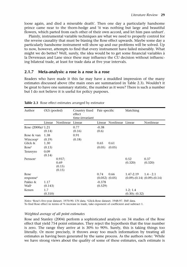
loose again, and died a miserable death'. Then one day a particularly handsomeprince came near to the thorn-hedge and 'it was nothing but large and beautifulflowers, which parted from each other of their own accord, and let him pass unhurt'.
Plainly, instrumental variable techniques are what we need to properly control forthe reverse causality that must be biasing the Rose effect upwards. Maybe some day aparticularly handsome instrument will show up and our problems will be solved. Upto now, however, attempts to find that every instrument have failed miserably. Whatmight we do better? Well, surely, the idea would be to get some financial variables àla Devereaux and Lane since these may influence the CU decision without influenc-ing bilateral trade, at least for trade data at five year intervals.
2.1.7 Meta-analysis: a rose is a rose is a rose
Readers who have made it this far may have a muddled impression of the manyestimates discussed above (the main ones are summarized in Table 2.3). Wouldn't itbe great to have one summary statistic, the number as it were? There is such a numberbut I do not believe it is useful for policy purposes.
Weighted average of all point estimates
Rose and Stanley (2004) perform a sophisticated analysis on 34 studies of the Roseeffect that yield 754 point estimates. They reject the hypothesis that the true numberis zero. The range they arrive at is 30% to 90%. Surely, this is taking things tooliterally. Or more precisely, it throws away too much information by treating allestimates as having been generated by the same process. As the authors note: 'Whilewe have strong views about the quality of some of these estimates, each estimate is
Literature Review 29
Table 2.3 Rose effect estimates arranged by estimator
Author OLS (pooled) Country fixed Pair specific Matchingeffect time-invariant
Linear Nonlinear Linear Linear Nonlinear Linear Nonlinear
Rose (2000a)a 1.21 0.77 -0.38(0.14) (0.16) (0.6)
Rose & van 1.38 0.91Wincoopa (0.19) (0.18)Glick & 1.30 0.65 0.61Roseb (0.13) (0.05) (0.05)Tenreyro 0.09
(0.14)Perssona 0.937; 0.52 0.37
0.69 (0.320) (0.320)(0.15)(0.15)
Rose 0.74 0.66 1.47-2.19 1.4 - 2.1responseb (0.052) (0.05) (0.09)-(0.14) (0.09)-(0.14)Pakko & 1.17 -0.378Walla (0.143) (0.529)Kenen 1.7 1.2; 1.4
(0.310) (0.30); (0.32)
Notes: aRose's five-year dataset. 1970-90. UN data. bGlick-Rose dataset. 1948-97. IMF data. To find Rose effect in terms of % increase in trade, take exponent of coefficient and subtract 1.
weighted equally; alternative weighting schemes might be regarded as suspect.'Please, suspect! That's what empirical researchers get paid for. All the estimates inRose (2000a), for example, should be ignored except the difference-in-differenceestimator that roughly controls for the gold-medal mistake of gravity models. AndyRose himself showed that all of them were incorrect since the pooling assumptionsnecessary for them to make sense have been rejected by his papers with van Wincoopand Glick.
Moreover, the patently incorrect pooled estimates of the Rose effect all of whichare at least twice too big are generally repeated in the literature as a way of showingthat the author's dataset is sound in that it can reproduce the mistaken estimates inRose (2000a). In other words, authors repeat them as a form of benchmarking, not forpolicy relevance. The meta-analysis statistical techniques are fascinating, but I don'tbelieve they add anything to our knowledge. Deep down they are basically a weight-ed average of all point estimates that include many of the point estimates that havebeen proven to be false.
2.1.8 Lessons for the euro area from non-European experiences
I believe the cleanest estimates we have on non-European currency unions are thosethat use matching since these go a long way towards controlling for the omittedvariable bias, and for any bias from model mis-specification. All the other estimatesseem to have serious flaws that would bias them upward. On the original Rosedataset, Persson (2001) found the effect to be between 15% and 66%. Rose (2001a)found it to be between 21% and 43% on a much larger dataset. An informal meta-analysis on these four estimates would suggest a number like 30%. And we can bepretty sure that this is an overestimate since the matching procedure cannot controlfor reverse causality, and it seems extremely likely that the je-ne-sais-quoi factors thatlead nations to adopt each other's currency also tend to promote bilateral trade.
I believe, however, that the non-European evidence has essentially zero informa-tional content for the euro area apart from the fact that it is worth looking for a Roseeffect in Europe. The basic problem is that the non-European data are driven bynations that are very small, very poor and very open. Exactly because the currencyunion pairs in the data are so strange, we cannot use the 30% to predict the curren-cy union affect for any nation that is not strange in the same way.23 I guess this fallsinto the category of common sense. If you study the trade effects of a currency unionon very small, very poor and very open nations, then what you learn is how muchcurrency unions affect the trade of very small, very poor and very open nations. DidI repeat myself? Well, I guess that is why they call it common sense.
2.2 Empirical findings on the euro area
What matters is not the length of the wand, but the magic in the stick. (Hagrid to Harry Potter)
Most of the Rose effect literature treats currency unions as magic wands one touchand intra-currency-union trade flows rise between 5% and 1400%. The only questionis: 'How big is the magic?' This approach was understandable when the literature wasdealing with hundreds of pairs of trade among CU members. Given the amazingrange of peculiar situations under study ranging from France's trade with itsoverseas departments to trade between the two tiny Pacific islands Nauru and Tuvalu one was naturally attracted by generalizations.
30 In or Out: Does It Matter?

In Europe, however, the big-magic approach is most definitely not good enough.We know an awful lot about the affected countries, far too much to pretend that theeuro will affect all their trade flows in the same way. Moreover, the euro matters fartoo much for easy generalizations to be appropriate. Some 290 million people use theeuro, and euro monetary policy quite directly touches the lives of another 200 mil-lion people living in the non-euro area EU nations and near neighbours.
Empirical studies of the euro's trade impact 24
Given the roaring interest sparked by Rose's papers, it was inevitable that someonewould try to estimate the Rose effect for the euro area. In April 2002, Andy Rosealerted the Managing Editors of Economic Policy to what appears to be the first paperon the subject.25 When I got this message, I looked up the paper and saw it was verymuch in the how-big-is-the-magic line not at all what we thought the world needed,but we asked the authors to write a paper that would go much further and after someiteration, commissioned what was eventually published as Micco, Stein and Ordoñez(2003b), or MSO for short. After a massive revision of its first draft, the paper waspresented to the October 2000 Economic Policy Panel Meeting hosted by the Bank ofGreece.
The Economic Policy panellists were quite positive on the paper and its main con-clusion that the euro had already boosted trade, but they had many questions andsuggestions. In their second revision, the authors addressed almost all these concerns.After a thorough edit, MSO was published in the April 2003 issue of Economic Policy an issue in which all articles dealt with the euro's impact.26
2.2.1 MSO (2003b)
The earliest version of MSO presented estimates of the Rose effect in the order ofabout 25%. These were so big that the referees and editors asked them to plot the dataand see if it appeared even without conditioning for other trade-enhancing factors.The result is shown in Figure 2.9.
It is somewhat hard to see what is going on when the data are plotted from 1980to 2002 (the latest data point MSO had), but in the right panel, the same data are plot-ted from 1993 to 2002. Note that there was a major change in the way the EU col-lected its trade data from 1993, so it is difficult to compare pre- and post-1993 figures.(Much more on this below.) In the right panel, there does indeed seem to be somesort of break in the data. But again, it is not that the touch of the euro's magic wandmade trade jump up by 25%. What happened was that the euro area's trade witheveryone fell as did trade among other developing nations at the time but theintra-euro area trade fell by less. Gomes et al. (2004) show a very similar graph, addingthe data for 2003, and find similar results. Flam and Nordström (2003) plot moredetailed data, showing the euro area's exports to other nations (eight other OECDnations) separately from the other-eight's exports to the euro area. The results inFigure 2.10 confirm the basic message but rely solely on export data.
The time-series are suggestive, but since bilateral trade is influenced by manythings that vary over time, especially incomes, MSO estimate a gravity model on datafrom 1992 to 2002 for two samples, one that is quite homogeneous (only the 15 EUnations) and one with 22 developed countries that is less so.
Rose effect estimates for the euro area, 6% more trade
The cleanest results in the MSO paper are estimates done with pair fixed effects onthe EU15 sample for the 1992 to 2002 period. Using this technique, MSO find thatthe Rose effect induced 6% more trade among euro area members.27 This estimation
Literature Review 31
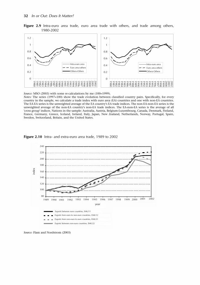
32 In or Out: Does It Matter?
0
0.2
0.4
0.6
0.8
1
1.2
19801981198219831984198519861987198819891990199119921993199419951996199719981999200020012002
Intra-euro area
Euro area-others
Others-Others
0
0.2
0.4
0.6
0.8
1
1.2
19801981198219831984198519861987198819891990199119921993199419951996199719981999200020012002
Intra-euro area
Euro area-others
Others-Others
Figure 2.9 Intra-euro area trade, euro area trade with others, and trade among others, 1980-2002
Source: MSO (2003) with some re-calculations by me (100=1999).Notes: The series (1997=100) show the trade evolution between classified country pairs. Specifically, for everycountry in the sample, we calculate a trade index with euro area (EA) countries and one with non-EA countries.The EA-EA series is the unweighted average of the EA country's EA trade indices. The non-EA-non-EA series is theunweighted average of the non-EA country's non-EA trade indices. The EA-non-EA series is the average of all'cross group' indices. Nations in the sample: Australia, Austria, Belgium-Luxembourg, Canada, Denmark, Finland,France, Germany, Greece, Iceland, Ireland, Italy, Japan, New Zealand, Netherlands, Norway, Portugal, Spain,Sweden, Switzerland, Britain, and the United States.
Figure 2.10 Intra- and extra-euro area trade, 1989 to 2002
Source: Flam and Nordstrom (2003)
1989 1990 1991 1992 1993 1994 1995 1996 1997 1998 1999 2000 2001 2002
year
240
220
200
160
140
120
100
80
inde
x
180
Exports between euro countries, EMU11
Exports from euro to non-euro countries, EMU12
Exports from non-euro to euro countries, EMU21
Exports between non-euro countries, EMU22
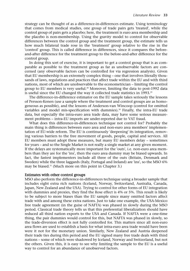
strategy can be thought of as a difference-in-differences estimate. Using terminologythat comes from medical studies, one group of trade pairs gets 'treated', while thecontrol group of pairs gets a placebo; here, the treatment is euro area membership andthe placebo is non-membership. Using the gravity model to control for observabledifferences between the control group and the treatment group, the estimate tells ushow much bilateral trade rose in the 'treatment' group relative to the rise in the'control' group. This is called difference in differences, since it compares the before-and-after difference for the treatment group to the before-and-after difference for thecontrol group.
In doing this sort of exercise, it is important to get a control group that is as com-parable as possible to the treatment group as far as unobservable factors are con-cerned (any observable factors can be controlled for via regression analysis). Giventhat EU membership is an extremely complex thing one that involves literally thou-sands of laws, regulations and practices that affect trade within the EU and with thirdnations, most of which are unobservable to the econometrician limiting the controlgroup to EU members is very useful.28 Moreover, limiting the data to post-1992 datais useful since the EU changed the way it collected trade statistics in 1993.29
The difference-in-difference estimator on the EU sample takes seriously the lessonsof Persson-Kenen (use a sample where the treatment and control groups are as homo-geneous as possible), and the lessons of Anderson-van Wincoop (control for omittedvariables and model mis-specification with dummies).30 Finally, the intra-EU tradedata, but especially the intra-euro area trade data, may have some serious measure-ment problems intra-EU imports are under-reported due to VAT fraud.
What does this difference-in-differences technique not control for? Probably themain thing is differences between euro area and non-euro area members' implemen-tation of EU-wide reform. The EU is continuously 'deepening' its integration, remov-ing various barriers to the free movement of goods, people, capital and services. AllEU members must adopt these measures, but many EU members delay sometimesfor years and so the Single Market is not really a single market at any given moment.If the delays are systematically more important for the 'outs', i.e. non-euro area mem-bers than they are for the 'ins', then the euro area dummy may be biased upwards. Infact, the fastest implementers include all three of the outs (Britain, Denmark andSweden) while the three laggards (Italy, Portugal and Ireland) are 'ins', so the MSO 6%may be biased.31 (Much more on this point in Chapter 3.)
Estimates with other control groupsMSO also perform the difference-in-differences technique using a broader sample thatincludes eight extra rich nations (Iceland, Norway, Switzerland, Australia, Canada,Japan, New Zealand and the USA). Trying to control for other forms of EU integrationwith dummies and proxies, they find the Rose effect is 4% or 5%. This result is likelyto be subject to more biases than the EU sample since many omitted factors affecttrade with and among these extra nations. Just to take one example, the USA-Mexicofree trade agreement (in the guise of NAFTA) was phased in slowly during the MSOperiod. Classical trade theory tells us that this preferential liberalization should havereduced all third nation exports to the USA and Canada. If NAFTA were a one-timething, the pair dummies would control for this, but NAFTA was phased in slowly, sothe trade-diversion effect is not fully controlled for. This matters since all non-euroarea flows are used to establish a basis for what intra-euro area trade would have beenwere it not for the monetary union. Similarly, New Zealand and Austria deepenedtheir trade ties during this period and the EU signed many free trade deals with thirdnations some of which were shadowed by Iceland, Norway and Switzerland, but notthe others. Given this, it is easy to see why limiting the sample to the EU is a usefulway to control for an abundance of unobserved factors.
Literature Review 33
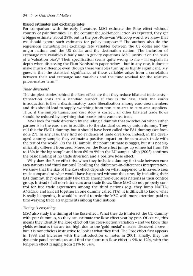
Biased estimates and exchange ratesFor comparison with the early literature, MSO estimate the Rose effect withoutcountry or pair dummies, i.e. the commit the gold-medal error. As expected, they geta bigger estimate, about 28%, but in the post-Rose-van Wincoop world, we know thatwe should ignore such estimates for policy purposes.32 The authors also do theregressions including real exchange rate variables between the US dollar and theorigin nation, and the US dollar and the destination nation. The inclusion ofexchange rate variables is fairly rare in gravity equations. MSO justify it on the basisof a 'valuation bias'.33 Their specification seems quite wrong to me I'll explain indepth when discussing the Flam-Nordström paper below but in any case, it doesn'tmake much difference even though these variables turn up as highly significant. Myguess is that the statistical significance of these variables arises from a correlationbetween their real exchange rate variables and the time residual for the relative-prices-matter term.34
Trade diversion?
The simplest stories behind the Rose effect are that they reduce bilateral trade costs transaction costs are a standard suspect. If this is the case, then the euro'sintroduction is like a discriminatory trade liberalization among euro area membersand this should lead to supply switching from non-euro area to euro area suppliers.Thus, if the simple transaction cost story is correct, all other bilateral trade flowsshould be reduced by anything that boosts intra-euro area trade.
MSO look for trade diversion by including a dummy that switches on when eitherpartner is in the euro area in addition to the standard currency union dummy. Theycall this the EMU1 dummy, but it should have been called the EA1 dummy (see foot-note 27). In any case, they find no evidence of trade diversion. Indeed, in the devel-oped country sample, they estimate a positive impact on the euro area's trade withthe rest of the world. On the EU sample, the point estimate is bigger, but it is not sig-nificantly different from zero. Moreover, the Rose effect jumps up somewhat from 4%to 13% in the big sample and from 6% to 9% in the EU sample. Alho (2002) confirmsthe basic finding of no trade diversion and a positive Rose effect.
Why does the Rose effect rise when they include a dummy for trade between euroarea nations and third nations? Recalling the difference-in-differences interpretation,we know that the size of the Rose effect depends on what happened to intra-euro areatrade compared to what would have happened without the euros. By including theirEA1 dummy, they essentially take trade among non-euro area nations as their controlgroup, instead of all non-intra-euro area trade flows. Since MSO do not properly con-trol for free trade agreements among the third nations (e.g. they lump NAFTA,ANZCER, and EER all together in one dummy called FTA), it is difficult to know whatis really happening. It would be useful to redo the MSO with more attention paid totime-varying trade arrangements among third nations.
Timing is everything
MSO also study the timing of the Rose effect. What they do is interact the CU dummywith year dummies, so they can estimate the Rose effect year by year. Of course, thismeans they identify the Rose effect off the cross-section variation and we know thisyields estimates that are too high due to the 'gold-medal' mistake discussed above but it is nonetheless instructive to look at what they find. The Rose effect first appearsin 1998 and increases with the introduction of notes in 2001. Finally, they usedynamic panel techniques and find the short-run Rose effect is 9% to 12%, with thelong-run effect ranging from 21% to 34%.
34 In or Out: Does It Matter?
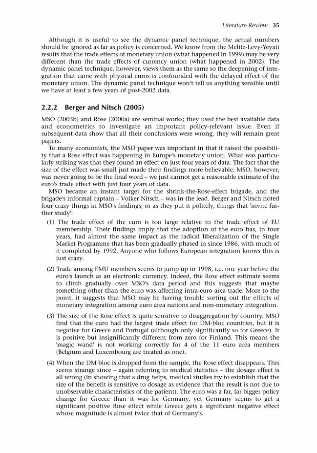
Although it is useful to see the dynamic panel technique, the actual numbersshould be ignored as far as policy is concerned. We know from the Melitz-Levy-Yeyatiresults that the trade effects of monetary union (what happened in 1999) may be verydifferent than the trade effects of currency union (what happened in 2002). Thedynamic panel technique, however, views them as the same so the deepening of inte-gration that came with physical euros is confounded with the delayed effect of themonetary union. The dynamic panel technique won't tell us anything sensible untilwe have at least a few years of post-2002 data.
2.2.2 Berger and Nitsch (2005)
MSO (2003b) and Rose (2000a) are seminal works; they used the best available dataand econometrics to investigate an important policy-relevant issue. Even ifsubsequent data show that all their conclusions were wrong, they will remain greatpapers.
To many economists, the MSO paper was important in that it raised the possibili-ty that a Rose effect was happening in Europe's monetary union. What was particu-larly striking was that they found an effect on just four years of data. The fact that thesize of the effect was small just made their findings more believable. MSO, however,was never going to be the final word we just cannot get a reasonable estimate of theeuro's trade effect with just four years of data.
MSO became an instant target for the shrink-the-Rose-effect brigade, and thebrigade's informal captain Volker Nitsch was in the lead. Berger and Nitsch notedfour crazy things in MSO's findings, or as they put it politely, things that 'invite fur-ther study':
(1) The trade effect of the euro is too large relative to the trade effect of EUmembership. Their findings imply that the adoption of the euro has, in fouryears, had almost the same impact as the radical liberalization of the SingleMarket Programme that has been gradually phased in since 1986, with much ofit completed by 1992. Anyone who follows European integration knows this isjust crazy.
(2) Trade among EMU members seems to jump up in 1998, i.e. one year before theeuro's launch as an electronic currency. Indeed, the Rose effect estimate seemsto climb gradually over MSO's data period and this suggests that maybesomething other than the euro was affecting intra-euro area trade. More to thepoint, it suggests that MSO may be having trouble sorting out the effects ofmonetary integration among euro area nations and non-monetary integration.
(3) The size of the Rose effect is quite sensitive to disaggregation by country. MSOfind that the euro had the largest trade effect for DM-bloc countries, but it isnegative for Greece and Portugal (although only significantly so for Greece). Itis positive but insignificantly different from zero for Finland. This means the'magic wand' is not working correctly for 4 of the 11 euro area members(Belgium and Luxembourg are treated as one).
(4) When the DM bloc is dropped from the sample, the Rose effect disappears. Thisseems strange since again referring to medical statistics the dosage effect isall wrong (in showing that a drug helps, medical studies try to establish that thesize of the benefit is sensitive to dosage as evidence that the result is not due tounobservable characteristics of the patient). The euro was a far, far bigger policychange for Greece than it was for Germany, yet Germany seems to get asignificant positive Rose effect while Greece gets a significant negative effectwhose magnitude is almost twice that of Germany's.
Literature Review 35

Shifting from critique to contribution, Berger and Nitsch add a fifth year of data(namely 2003), and re-estimate MSO using recently revised trade data. Interestingly,both the data revision and extra year seem to greatly increase the Rose effect. (Below,I'll argue that this is a sign that, as Marcellus said so eloquently when Hamlet slippedoff for a tête-à-tête with a ghost, 'Something is rotten in the state of Denmark'.)
They also put the adoption of the euro in historical perspective, viewing the euroarea as 'a continuation, or culmination, of a series of policy changes that have ledover the last five decades to greater economic integration among the countries thatnow constitute the [euro area]'. Specifically, they use data for MSO's developed coun-try sample of the EU15 plus eight reaching back to 1948! Their bottom line is thatthrowing in a time-trend-dummy for trade among the 11 euro area members wipesout the Rose effect completely. There is surely something to the euro area-as-a-con-tinuum idea see Mongelli, Dorrucci and Agur (2005) for a more elaborate formal-ization of the idea that European trade and policy integration are a dialectic process and this surely makes it hard to separate the Rose effect from the effects of otherintegration initiatives. However, I think it is too blunt to throw in a time trend forthe euro area 12. European integration has affected all EU members equally. In futuredrafts, I hope the authors will repeat more of the MSO robustness checks with theirupdated data, and redo the time trend exercise, but with a trend for EU membershipas a whole. It would also be interesting to see if they could develop a data-based indexof extraordinarily close integration among the DM bloc, rather than the EA12. Forexample, one might take estimates of bilateral pass-through elasticities as proxies forpair-specific trade integration, the notion being that pass through would be biggerbetween more tightly integrated partners.35
2.2.3 Flam and Nordström (2003)
This is probably the best paper in the field to date. It avoids the gold, silver andbronze medal mistakes that plague the rest of the papers in this literature. Moreover,they use a dataset that probably has far fewer data issues than those used by MSO andtheir followers, namely they use bilateral exports rather than an average of bilateralexports and imports. The use of direction-specific bilateral trade flows is what thebasic gravity theory suggests should be used. Moreover, it allows them to look at anissue that concerns all the non-euro area nations, whether the euro puts theirexporters at a disadvantage in the euro area. Additionally, they also alert the readerto the problems with European trade data collection (much more on this below).Finally, they perform their regressions on sector data as well as aggregate data.
Their basic findings on the aggregate data are in line with MSO, both in terms ofsize and timing. Their preferred estimate uses the three non-euro area and eight extrarich nations as the control group and they find the Rose effect implies about 15%higher trade; euro area trade with other nations (in either direction) is boosted byabout half that. When they use the cleanest definition of the control group otherEU nations the Rose effect is only 9%. Their findings on the sectoral data suggestthat the Rose effect is only present in sectors marked by differentiated products, con-firming the earlier results of Taglioni (2002), and Baldwin, Skudelny and Taglioni(2005 ).
There are a few puzzling findings in Flam-Nordström. As in MSO, they find thatthe Single Market has about the same magnitude effect on trade as the euro. Also,they find that the Rose effect is larger in the broader sample of nations. When theyrun their preferred estimate on EU nations only, the Rose effect drops more than twostandard deviations. Moreover, the estimate for the exports of non-euro area nationsto euro area nations is almost identical to the intra-euro area effect, while the euro
36 In or Out: Does It Matter?

area's exports to non-euro area nations seem to be unaffected by the new currency.This finding is both intriguing and suspicious. The intriguing part is that if it is real-ly coming from the euro's introduction, then the euro must be making it easy, cheap-er and/or safer to sell to euro area nations. Or to put it differently, the euro makes theeuro area members extraordinarily good importers, rather than extraordinarily goodexporters. It is suspicious since it suggests that it is not really the euro that is behindit all, but rather something that the euro area nations, or a subset of them, did aroundthe time of the euro something that made their markets more open to imports fromall other EU nations.
Another hint that it may not have been the euro causing the big trade effect comesfrom the authors' experiments with the sample. The estimate of the intra-euro areadummy jumps up by about one standard deviation when the sample includes Norwayand Switzerland in addition to the EU14 (Flam and Nordström seem to excludeGreece from their aggregate regressions since they lacked Greek data for the sectorregressions). Moreover, the dummy on euro area exports to non-EA nations alsojumps up, by two standard deviations. What could this mean?
Recall the difference-in-differences interpretation of the model estimated with pairdummies (a separate one for each direction-specific bilateral export). The treatmentgroups in all cases are intra-EA trade flows. What changes with the sample is the con-trol group. In the EU sample, the control group is the six trade flows among the three'outs', i.e. non-EA members, Britain, Denmark and Sweden, since Flam andNordström include dummies for all trade flows between the ins and outs. Adding inNorway and Switzerland brings the total up to 20 control pairs. The fact that the EAdummy estimate rises so much reflects the fact that trade between Norway andSwitzerland and between these nations and the outs did not rise as much as tradeamong the outs did during this period. That in itself suggests that some strongly pro-trade factor omitted from the regression was stimulating trade among EU members,regardless of the euro usage. The authors do include an EEA dummy (which standsfor the European Economic Area agreement whose goal is to extend the single mar-ket to Norway and Iceland), so this should have been controlled for, but they maystill be missing something. The leftmost bar in Figure 2.11 shows the year by year EAdummy; the other bar in each pair of bars shows the estimated EU dummy (actuallyit is the EEA dummy even though they call it the EU dummy). What we see is thatjust as the Rose effect is estimated to be increasing sharply, in the 1999 to 2001 peri-od, the effectiveness of the single market is estimated as diminishing by almost asmuch. The line shows the sum of the two. This also 'explains' why De Souza (2002)finds no Rose effect when he includes a time trend for EU integration, and why Bergerand Nitsch (2005) are able to shrink the Rose effect to nothing by including a timetrend for integration among the eventual euro area members.
All this invites further study, as Berger and Nitsch would say. It might also be inter-esting to interact an estimated EU integration trend with individual members' trans-position deficits (i.e. the extent to which they are behind in implementing EU direc-tives). It is worrying that the outs and the ins are so different when it comes to trans-position in the face of rising overall integration. It would also be interesting to see thesensitivity to period with the EU sample alone.
Exchange rates and gravity. But does it work in theory?
One of the methodological innovations in Flam and Nordström is their treatment ofexchange rates. The inclusion of exchange rates is important to control one of thepotential sources of spurious Rose effects in the euro data. As the euro droppedsharply at birth, the intra-euro area goods came to look cheap compared to thirdnation goods, US goods in particular. In other words, the exchange rate altered
Literature Review 37
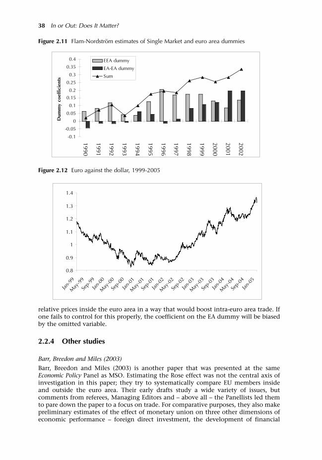
relative prices inside the euro area in a way that would boost intra-euro area trade. Ifone fails to control for this properly, the coefficient on the EA dummy will be biasedby the omitted variable.
2.2.4 Other studies
Barr, Breedon and Miles (2003)
Barr, Breedon and Miles (2003) is another paper that was presented at the sameEconomic Policy Panel as MSO. Estimating the Rose effect was not the central axis ofinvestigation in this paper; they try to systematically compare EU members insideand outside the euro area. Their early drafts study a wide variety of issues, butcomments from referees, Managing Editors and above all the Panellists led themto pare down the paper to a focus on trade. For comparative purposes, they also makepreliminary estimates of the effect of monetary union on three other dimensions ofeconomic performance foreign direct investment, the development of financial
38 In or Out: Does It Matter?
0.8
0.9
1
1.1
1.2
1.3
1.4
Jan-9
9
May
-99
Sep-
99
Jan-0
0
May
-00
Sep-
00
Jan-0
1
May
-01
Sep-
01
Jan-0
2
May
-02
Sep-
02
Jan-0
3
May
-03
Sep-
03
Jan-0
4
May
-04
Sep-
04
Jan-0
5
-0.1
-0.05
0
0.05
0.1
0.15
0.2
0.25
0.3
0.35
0.4
1990
1991
1992
1993
1994
1995
1996
1997
1998
1999
2000
2001
2002
Dum
my
coef
fici
ents
EEA dummy
EA-EA dummy
Sum
Figure 2.11 Flam-Nordström estimates of Single Market and euro area dummies
Figure 2.12 Euro against the dollar, 1999-2005
markets and overall macroeconomic performance though they recognize that theirability to control for other factors is more limited for these other indicators.36 Theseauthors make a much more thorough attempt than MSO to correct for reversecausality. Even after this correction, however, they note that the Rose effect is positiveand significant.
Bun and Klaassen (2002)
One of the other papers in line for the I-did-it-first prize is Bun and Klaassen (2002),since their first draft was circulated in 2001. This paper employs a dynamic fixedeffects estimator. The results they obtain are quite similar to those reported for MSOusing a similar estimator.
De Souza (2002), Piscitelli (2003) and De Nardis and Vicarelli (2003a)
De Souza (2002) estimates the basic gravity model for the EU15 countries with theaddition of a time trend. He finds no evidence for a significant Rose effect unless heremoves the trend. This result is interesting, maybe even important, but throwinglinear terms can do lots of things to a regression that gets most of its traction fromthe time-variation of the policy variable of interest. MSO's experiments with timetrends (in the first draft) and a direct measure of EU integration in the publishedversion do not line up with De Souza's findings.
Piscitelli (2003), following the 2001 draft of MSO, finds that lengthening the sam-ple back to 1980 reduces the Rose effect estimates. The paper also finds that the sizeof the Rose effect changes with the data used. OECD trade data uses the 'cost, insur-ance and freight' (cif) methodology while the IMF trade data used in MSO (2003)takes the 'free on board' (fob) approach. I'll have much more to say about this result,but I note here that fob is what you get when you rely on the exporter's data and cifwhen you rely on the importer's data (for most nations, the UN's ComTrade database the fount of all trade data has four observations on bilateral trade, e.g. France toGermany as reported by the French and Germans, and Germany to France again byboth nations; MSO average all of these to get their one estimate of bilateral trade).
De Nardis and Vicarelli (2003a) was also one of the early papers on this. (One ofthe reasons Economic Policy decided to commission MSO was that others had foundsimilar results.) They take a different tack at controlling for reverse causality, but getabout the same answer as MSO; 10% in the short run and 20% in the long run.
Anderton, Baltagi, Skudelny and De Souza (2002)
This paper uses more sophisticated econometrics three-stage least squares toestimate import demand functions. They find no direct evidence of a Rose effect, butgiven the relatively small number of post-euro observations, it is hard to know whatto make of this. Given the good data on Europe, however, this more direct approachto estimating the euro's impact should probably be tried again.
Mancini-Griffoli and Pauwels (2006)
One very recent paper uses sophisticated econometrics to identify the timing of thestructural break caused by the euro. The authors develop a panel-data version of therecent end-of-sample structural break test suggested by Andrews (2003). This allowsthem to explicitly deal with the fact that there are very few data observations afterthe euro's introduction. The test avoids the need to make assumptions about thedistributions of errors by building a test-statistic whose distribution is estimated usingparametric subsampling techniques. One key novelty is that the power of the testallows the authors to test for short-lived breaks.
Their findings confirm those of some of some papers in the field but contradict
Literature Review 39
others. First, they find that the euro did have a positive impact on trade with theeffect being first felt break in the first quarter of 1999. Second, they find that thestructural break is short-lived, lasting only up to mid-2001. Third, they find no evi-dence that the euro affected the trade of non-euro area nations a result that con-trasts with MSO (2003) and Flam and Nordström (2003) who find a positive effect fornon-euro area nations.
2.3 Did the euro affect trade pricing?
The standard Mundellian optimal-currency-area story has multiple currencies actingas transaction costs what is often called a 'frictional' trade barrier (something like atariff where the tariff revenue is thrown away). If this traditional view is correct, thenwe should observe a significant impact of the euro on trade pricing. In particular, tothe extent that currency-linked transaction costs are important, adoption of acommon currency should narrow international price differences with the currencyunion, but not between the currency union and the rest of the world. More moderntheories of international pricing suggest that price dispersion is limited by an'arbitrage band' whose width may be related to exchange rate volatility and commoncurrency (Baldwin, 1991; Baldwin and Taglioni, 2005).
So what do the data say? While the empirical literature on the euro's trade pricing impact is severely under-
developed compared to the trade flow literature, a string of recent studies suggest thatthe euro has affected trade pricing. This is a very recent development since one earlyand very influential study on this question Engel and Rogers (2004) suggested thatthe euro had had no impact. One major problem in this literature stems from the lackof a standard, well-estimated and widely agreed model of what trade pricing shouldlook like. Without this trade-price-equivalent of the gravity model, the studies are dif-ficult to interpret and compare.
We start with the papers that support the notation that the euro has had an impacton trade pricing, in particular by narrowing the price dispersion among members ofthe euro area.
2.3.1 Allington, Kattuman and Waldmann (2005)
Allington et al. (2005) is the best paper in the field to date, in my opinion. Theauthors focus on a measure of price dispersion, comparing the pre-euro and post-eurobehaviour of their measure for nations that are inside the euro area and nations thatare not. To control partly for many other integrating policy changes, they limit theuniverse to members of the EU15. They find robust results which show that the eurosignificantly lowered price dispersion within the euro group. The data they use iseurostat's 'Comparative price level indices' for individual consumption expenditure inabout 200 product groups for all EU15 countries during 1995-2002 (annual data).
The authors also report that there was not a sudden change in dispersion, but thatthe euro's introduction accelerated the declining dispersion that was ongoing duringthe 1990s (the 1990s was marked by substance market integration in the EU).Moreover, they find enormous differences across product categories. This sort ofcross-sector variation is perfectly normal in disaggregated data, but it highlights thefact that the euro's impact on economic activity is surely different in different sectors.
The key to the authors' finding is a difference-in-difference result of the sort thatwas discussed at length in Section 2.1. The basic idea is to see whether the change indispersion between the pre- and post-euro periods (the 'difference') is substantially
40 In or Out: Does It Matter?
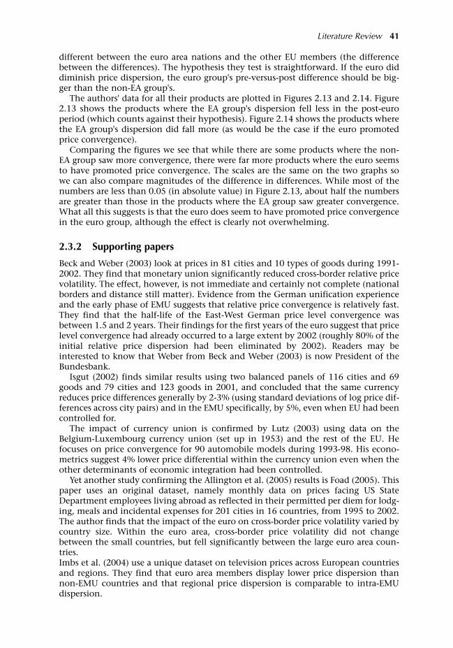
different between the euro area nations and the other EU members (the differencebetween the differences). The hypothesis they test is straightforward. If the euro diddiminish price dispersion, the euro group's pre-versus-post difference should be big-ger than the non-EA group's.
The authors' data for all their products are plotted in Figures 2.13 and 2.14. Figure2.13 shows the products where the EA group's dispersion fell less in the post-europeriod (which counts against their hypothesis). Figure 2.14 shows the products wherethe EA group's dispersion did fall more (as would be the case if the euro promotedprice convergence).
Comparing the figures we see that while there are some products where the non-EA group saw more convergence, there were far more products where the euro seemsto have promoted price convergence. The scales are the same on the two graphs sowe can also compare magnitudes of the difference in differences. While most of thenumbers are less than 0.05 (in absolute value) in Figure 2.13, about half the numbersare greater than those in the products where the EA group saw greater convergence.What all this suggests is that the euro does seem to have promoted price convergencein the euro group, although the effect is clearly not overwhelming.
2.3.2 Supporting papers
Beck and Weber (2003) look at prices in 81 cities and 10 types of goods during 1991-2002. They find that monetary union significantly reduced cross-border relative pricevolatility. The effect, however, is not immediate and certainly not complete (nationalborders and distance still matter). Evidence from the German unification experienceand the early phase of EMU suggests that relative price convergence is relatively fast.They find that the half-life of the East-West German price level convergence wasbetween 1.5 and 2 years. Their findings for the first years of the euro suggest that pricelevel convergence had already occurred to a large extent by 2002 (roughly 80% of theinitial relative price dispersion had been eliminated by 2002). Readers may beinterested to know that Weber from Beck and Weber (2003) is now President of theBundesbank.
Isgut (2002) finds similar results using two balanced panels of 116 cities and 69goods and 79 cities and 123 goods in 2001, and concluded that the same currencyreduces price differences generally by 2-3% (using standard deviations of log price dif-ferences across city pairs) and in the EMU specifically, by 5%, even when EU had beencontrolled for.
The impact of currency union is confirmed by Lutz (2003) using data on theBelgium-Luxembourg currency union (set up in 1953) and the rest of the EU. Hefocuses on price convergence for 90 automobile models during 1993-98. His econo-metrics suggest 4% lower price differential within the currency union even when theother determinants of economic integration had been controlled.
Yet another study confirming the Allington et al. (2005) results is Foad (2005). Thispaper uses an original dataset, namely monthly data on prices facing US StateDepartment employees living abroad as reflected in their permitted per diem for lodg-ing, meals and incidental expenses for 201 cities in 16 countries, from 1995 to 2002.The author finds that the impact of the euro on cross-border price volatility varied bycountry size. Within the euro area, cross-border price volatility did not changebetween the small countries, but fell significantly between the large euro area coun-tries.Imbs et al. (2004) use a unique dataset on television prices across European countriesand regions. They find that euro area members display lower price dispersion thannon-EMU countries and that regional price dispersion is comparable to intra-EMUdispersion.
Literature Review 41

42In or O
ut: Does It M
atter?
-0.25 -0.2 -0.15 -0.1 -0.05 0
Edible ice, ice cream and sorbetSolid fuels
Other tobacco productsTea and other infusions
Pets and related productsWine, cider and perry
Other edible oils and fatsGlassware and ceramic ware for households, offices and
Fruit and vegetable juicesDelicatessen and other meat preparations
Living-room and dining-room furnitureJewellery, clocks and watches
Fuels and lubricants for personal transport equipmentPreserved milk
Jams, marmalades and honeyPharmaceutical products
Food products n.e.c.Bicycles
Fortified and sparkling wineBeef
Other milk productsMiscellaneous printed matter
Carpets and other floor coveringsElectric appliances for personal care
Major durables for outdoor recreationFresh or chilled fruit
ButterDried fruit and nuts
Preserved or processed vegetables and vegetable-based productsSugar
Frozen fruit, preserved fruit and fruit-based productsVeal
Motor cars with petrol engine of cubic capacity of 3000cc and overPork
Household cleaning suppliesFresh or chilled vegetables other than potatoes
Other personal effects n.e.c.Kitchen furniture
Stationery and drawing materialsOther appliances, articles and products for personal care
Difference in difference
Figure 2.13 Panel A: Difference in differences, EA and non-EA EU members
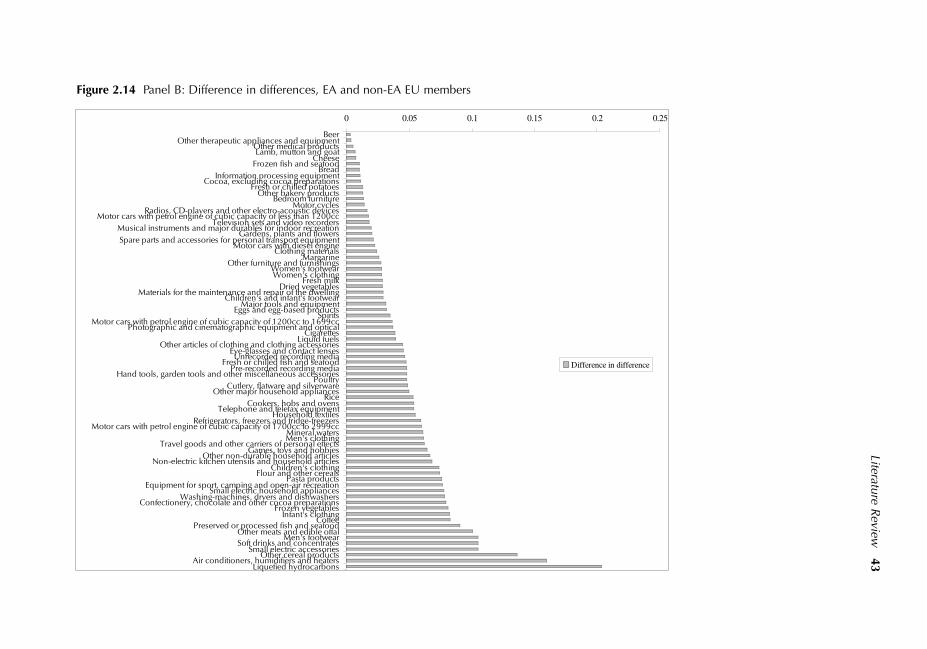
Literature Review
43
Figure 2.14 Panel B: Difference in differences, EA and non-EA EU members
0 0.05 0.1 0.15 0.2 0.25
BeerOther therapeutic appliances and equipment
Other medical productsLamb, mutton and goat
CheeseFrozen fish and seafood
BreadInformation processing equipment
Cocoa, excluding cocoa preparationsFresh or chilled potatoes
Other bakery productsBedroom furniture
Motor cyclesRadios, CD-players and other electro-acoustic devices
Motor cars with petrol engine of cubic capacity of less than 1200ccTelevision sets and video recorders
Musical instruments and major durables for indoor recreationGardens, plants and flowers
Spare parts and accessories for personal transport equipmentMotor cars with diesel engine
Clothing materialsMargarine
Other furniture and furnishingsWomen's footwearWomen's clothing
Fresh milkDried vegetables
Materials for the maintenance and repair of the dwellingChildren's and infant's footwear
Major tools and equipmentEggs and egg-based products
SpiritsMotor cars with petrol engine of cubic capacity of 1200cc to 1699cc
Photographic and cinematographic equipment and opticalCigarettes
Liquid fuelsOther articles of clothing and clothing accessories
Eye-glasses and contact lensesUnrecorded recording media
Fresh or chilled fish and seafoodPre-recorded recording media
Hand tools, garden tools and other miscellaneous accessoriesPoultry
Cutlery, flatware and silverwareOther major household appliances
RiceCookers, hobs and ovens
Telephone and telefax equipmentHousehold textiles
Refrigerators, freezers and fridge-freezersMotor cars with petrol engine of cubic capacity of 1700cc to 2999cc
Mineral watersMen's clothing
Travel goods and other carriers of personal effectsGames, toys and hobbies
Other non-durable household articlesNon-electric kitchen utensils and household articles
Children's clothingFlour and other cereals
Pasta productsEquipment for sport, camping and open-air recreation
Small electric household appliancesWashing-machines, dryers and dishwashers
Confectionery, chocolate and other cocoa preparationsFrozen vegetables
Infant's clothingCoffee
Preserved or processed fish and seafoodOther meats and edible offal
Men's footwearSoft drinks and concentrates
Small electric accessoriesOther cereal products
Air conditioners, humidifiers and heatersLiquefied hydrocarbons
Difference in difference

2.3.3 The odd man out: Engel and Rogers (2004)
When the Economic Policy Managing Editors decided in April 2002 to do a wholePanel on the euro's effects, one natural topic was the euro's impact on trade prices.We eventually got Charles Engel, Michel Knetter and John Rogers to agree to do apaper on the topic, but the paper experienced a number of difficulties before it waseventually published in July 2004. Knetter had to withdraw as he became a Dean andneither Engel nor Rogers could make the euro-issue Panel, so the paper was notpublished with the others in the Economic Policy special issue on the euro that alsoappeared as the book by Baldwin, Bertola and Seabright (2003). The paper that waseventually published as Engel and Rogers (2004) was presented at the October 2003Economic Policy Panel in Rome. The Rome Panel was highly critical of the paper themain critiques were published in the Discussants' and Panellists' comments alongwith the paper so the Managing Editors asked for major revisions that delayed thepaper longer than Economic Policy's usual 6-months-after-the-panel rule. Even withthe delay, it was one of the first papers to look at the price effects using a significantnumber of post-euro observations.
Specifically, Engel and Rogers (2004) use data gathered by the EconomistsIntelligence Unit on consumers prices of 101 traded goods and 38 non-traded itemsin 18 European cities (11 in euro area countries and 7 in non-euro area countries) forthe years 1990-2003. This price data, which was collected to help firms decide uponthe cost-of-living adjustment they should offer to expatriate employees, concernsindividual goods and care is taken to ensure that the goods are comparable and theprices are for similar outlets (e.g. high-street stores in all the cities rather than largediscount chains in one city and a boutique store in another).
The authors find no evidence that the euro decreased price dispersion among euroarea members, although they do find that there has been a significant reduction inprice dispersion throughout the decade of the 1990s.
Why do Engel and Rogers (2004) find such different results? A look at their dataand the critique of one of their discussants at the Panel, Giovanni Veronese from theBank of Italy, is revealing. The authors take as their measure of price dispersion themean squared error of the log difference in prices between cities. The salient pointsfrom the cross-section aspect of the raw data are:
Price dispersion is greater among non-euro nations than it is among the Euro-11.
Price dispersion among both euro and non-euro nations is greater than membersof the DM bloc (a group that experienced very little exchange rate variability inthe 10 years leading up to the Euro's introduction).
Price dispersion across cities within a single nation is even lower than that of theDM bloc.
On the face of it, these cross-group comparisons suggest that the level of pricedispersion is roughly correlated with the degree of exchange rate variability.
The time series facts, however, seem to tell a different story. Price dispersion in allfour groups shows a clear decline in the early 1990s, but the decline stops around thetime of the euro's introduction. Indeed, it even seems to increase somewhat. Thus thetime-series facts seem to suggest that the euro had no impact on price dispersion, oreven raised the degree of dispersion.
The problem with this conclusion, and the main point of Giovanni Veronese, wasthat these results are not conditional on other factors. In particular, Veronese suggeststhat there was a powerful force driving increased dispersion in the post-1999 period,namely the divergence of national inflation rates in the euro area that occurred justafter the euro's launch.
44 In or Out: Does It Matter?

Literature Review 45
0
0.05
0.1
0.15
0.2
0.25
0.3
0.35
0.4
1990 1991 1992 1993 1994 1995 1996 1997 1998 1999 2000 2001 2002 2003
Mea
n S
quar
ed E
rror
Non-Euro-11 Europe
Euro-11
DM Bloc
Within country (Euro-11)
Figure 2.15 Engel and Rogers (2004), price dispersion data by group
Source: Engel and Rogers (2004), Figure 4
0.0
0.5
1.0
1.5
2.0
2.5
3.0
3.5
4.0
1990 1991 1992 1993 1994 1995 1996 1997 1998 1999 2000 2001
All Items Industrial goods excluding energy and food
(1) Excluding Greece and Luxembourg
Figure 2.16 Convergence and divergence of euro area inflation rates, 1990-2001
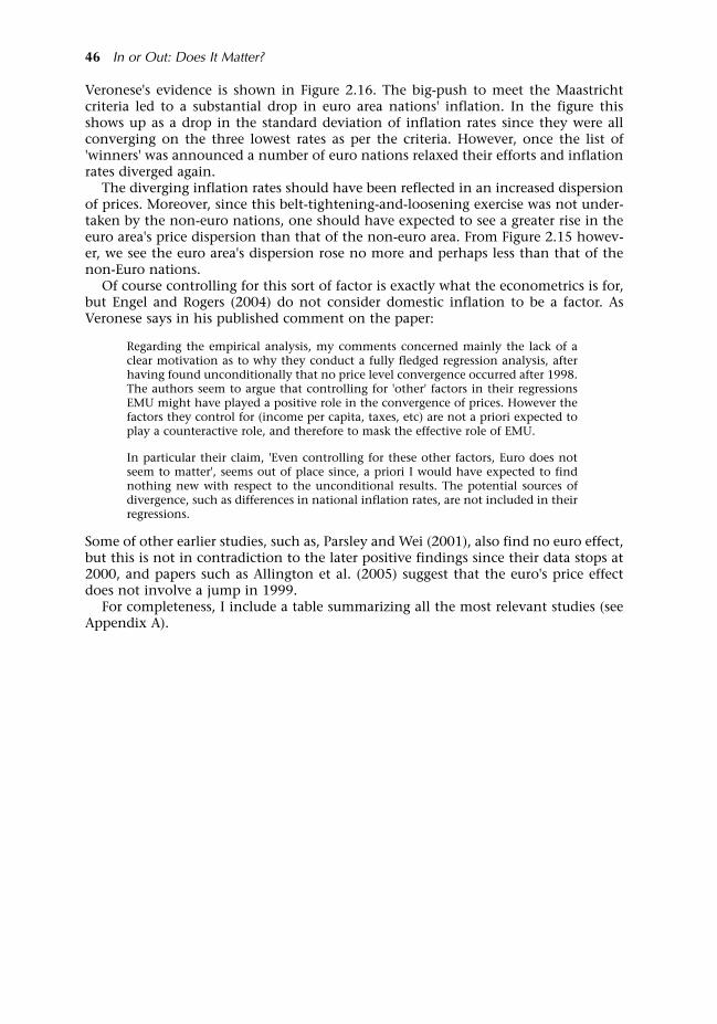
Veronese's evidence is shown in Figure 2.16. The big-push to meet the Maastrichtcriteria led to a substantial drop in euro area nations' inflation. In the figure thisshows up as a drop in the standard deviation of inflation rates since they were allconverging on the three lowest rates as per the criteria. However, once the list of'winners' was announced a number of euro nations relaxed their efforts and inflationrates diverged again.
The diverging inflation rates should have been reflected in an increased dispersionof prices. Moreover, since this belt-tightening-and-loosening exercise was not under-taken by the non-euro nations, one should have expected to see a greater rise in theeuro area's price dispersion than that of the non-euro area. From Figure 2.15 howev-er, we see the euro area's dispersion rose no more and perhaps less than that of thenon-Euro nations.
Of course controlling for this sort of factor is exactly what the econometrics is for,but Engel and Rogers (2004) do not consider domestic inflation to be a factor. AsVeronese says in his published comment on the paper:
Regarding the empirical analysis, my comments concerned mainly the lack of aclear motivation as to why they conduct a fully fledged regression analysis, afterhaving found unconditionally that no price level convergence occurred after 1998.The authors seem to argue that controlling for 'other' factors in their regressionsEMU might have played a positive role in the convergence of prices. However thefactors they control for (income per capita, taxes, etc) are not a priori expected toplay a counteractive role, and therefore to mask the effective role of EMU.
In particular their claim, 'Even controlling for these other factors, Euro does notseem to matter', seems out of place since, a priori I would have expected to findnothing new with respect to the unconditional results. The potential sources ofdivergence, such as differences in national inflation rates, are not included in theirregressions.
Some of other earlier studies, such as, Parsley and Wei (2001), also find no euro effect,but this is not in contradiction to the later positive findings since their data stops at2000, and papers such as Allington et al. (2005) suggest that the euro's price effectdoes not involve a jump in 1999.
For completeness, I include a table summarizing all the most relevant studies (seeAppendix A).
46 In or Out: Does It Matter?

While the size of the estimated euro area Rose effect does not strain credibility in thesame way as the bigger estimates in the earlier literature did, many questions remain.The speed with which the effect appears is suspicious, as is the fact that it appearedbefore 1999 according to several researchers. The lack of a trade diversion effect alsoraises questions.
It is always exciting to find something new and real, but one must also considerthe possibility that the effect is spurious. I believe there to be three hypotheses thatneed to be eliminated before we can be absolutely sure that the estimates are tellingus anything real about the economy.
VAT fraud created a spurious Rose effect.
Delayed effects of the euro depreciation created a spurious Rose effect.
Effects of euro area implementation of Internal Market measures create aspurious Rose effect.
These are considered in turn.
3.1 Lies, damned lies and statistics: VAT fraud
This section considers the very real possibility that the Rose effect in the euro area isa statistical illusion stemming from the way trade figures are gathered. This isheadache material, but I believe it is necessary since existing estimates of the effectsare of the same order of magnitude as the estimated Rose effects in the euro area.
One of the great coups of the 1986 Single European Act was to remove Europe'sinternal borders, at least as far as trade is concerned. This happened in 1993 andchanged the way trade statistics were gathered on intra-EU trade. Data on intra-EUtrade from 1993 onwards were collected by VAT authorities rather than customs offi-cers, since intra-EU trade no longer passed through customs frontiers.
Why would VAT authorities produce trade statistics? EU nations have VAT systemsthat are based on the so-called destination principle, i.e. a good pays the VAT rate ofthe nation where it is sold, not where it is made. Practically speaking, this means thatthe exporting EU nation rebates its VAT to the exporting firm and the importing EUmember imposes its own VAT rate on the importing firm. This is why VAT authoritieshave always kept track of imports and exports.
The problem is that this creates a direct link between trade date and tax avoidanceand evasion. Worse still, tax enforcement changes and anticipation of the same can create reactions that distort EU trade flows. These distortions can vary acrosstime, across trade pairs and commodities. Although the VAT system was massively
3 Is the Euro Area Rose Effect a SpuriousResult?
47

48 In or Out: Does It Matter?
reformed in anticipation of the suppression of border controls a major part of thisbeing a narrowing of differences in VAT rates the 1993 system was susceptible tofraud.
3.1.1 Fraud and intra-EU trade figures
As early as the mid-1990s, problems of VAT fraud were recognized, for example, bythe European Parliament's first Temporary Enquiry Committee in 1997. Measureswere taken to improve the system, but things were still problematic when the eurowas launched. A European Commission report to the Council and EuropeanParliament in 2000 used usually blunt language:
The transitional VAT arrangements have been in place for more than 6 years.During this period, one would have expected that the implementing problemsshould have been solved and that the system should be running smoothly.However, this does not appear to be the case. The 6 years appear to have given thefraudsters time to appreciate the possibilities offered by the transitional VATarrangements to make money, while, generally speaking, Member States have notmet the challenge posed by fraud. There are indications that the level of seriousfraud in intra-Community trade is growing.
The exact nature of such fraud is not easy to ascertain. Typically, it creates a gapbetween export statistics (every exporter wants the VAT rebate) and import statistics(some have an incentive to avoid paying the importing nation's VAT). But, it can alsoinflate the trade statistics as in the case of the so-called 'carousel fraud' (see Box 3.1).
Box 3.1: Acquisition and carousel fraud
The easiest fraud is called acquisition fraud. Criminals set up a company in, say, the UK andimport goods from Germany at a zero-VAT price (the selling company gets the Germany VATrebated). The importing firm sells the goods in Britain at something like the with-VAT price(since that is what honest importers have to charge) but they never pay the VAT; they go outof business before the VAT authorities can get them.
The carousel fraud takes this one step further, but understanding it requires some backgroundon why VAT is usually impervious to fraud. An EU firm that sells a good is liable for the VATon the full sales price, unless entrepreneurs can prove that they bought inputs to make thegood, in which case they only pay the VAT on their value added. The point is that the VAThas already been paid on the inputs. How do we know the VAT has been paid on inputs?Well, whether it was made locally or imported, the local VAT rate was paid. How do weknow that the firm won't exaggerate its purchases of inputs? Counteracting incentives is theanswer. The input seller would like to under-report its sales to reduce its VAT bill, but theinput buyer would like to over-report its purchases to reduce its VAT bill. The gain and lossare of identical magnitude, so there is no reason to suspect an upward or downward bias. Inshort, buyers and sellers become informants on each other as far as VAT payments are con-cerned. Now, how does this work with exports? Suppose the export shipment is to Belgiumand is worth £100,000. If the UK VAT rate is 20%, the British VAT authority pays the export-ing firm £20,000 - which is the amount of VAT that has been paid on the good in Britain.
But what if the VAT was never paid on the import into Britain because of an acquisition fraud?In this case, the criminals pocket £20,000, having paid very little, or maybe no VAT, inBritain. Since it worked once, they may be tempted to put the same goods through the samecycle again. The goods turn around and around like a carousel, each time showing up twiceas an export and once or never as an import.

3.1.2 The effect is huge and anti-fraud activity differs across time andcountry pairs
The effect of this fraud was so large that the UK had to restate its national accounts(see Ruffles et al., 2003). The revisions involve upward adjustments to imports of £1.7billion in 1999, £2.8 billion in 2000, £7.1 billion in 2001 and £11.1 billion in 2002.Unadjusted imports in 2002 were £220 billion, so the effect is about 5%. The problemis not limited to the UK as Figure 3.1 shows. The problem is large, on the order of 5%,and it varies over time. As inspection of the figure shows, the problem appears toincrease substantially in the run up to the Euro's introduction.
Policy reaction is correlated with the timing of the Euro's introduction. TheEuropean Commission has been coordinating the implementation of anti-fraud activ-ities since the 1990s, and these are still not complete. The rate of implementationvaries across nations and across types of trade. I presume the criminals involved inthis fraud follow the process carefully, so it is entirely possible that they alter theirbehaviour in anticipation of changes.
If this fraud were simple e.g. it consisted entirely of acquisition fraud, simple fixesmight work, for example, researchers could use export data. But as the carousel fraudsuggests, even these data may be exaggerated in ways that vary across time, countrypairs and commodities.
3.2 The Rotterdam effect
A huge fraction of Germany's imports from non-EU nations arrive via Rotterdam.Some of this trade is recorded as a Dutch import from, say, New Zealand and thenrecorded as a German import from the Netherlands. Some of it, however, is recordedas a German import from New Zealand since it is subject to a 'transit' regime by whichthe tariff and VAT are not paid until the good arrives in Germany. The system is calledthe TIR system ('Transports Internationaux Routiers') and it involves transferring
Is the Euro Area Rose Effect a Spurious Result? 49
1988 1989 1990 1991 1992 1993 1994 1995 1996 1997 1998 1999 2000 2001
Arrivals Dipatches
440
420
400
380
360
220
200
180
160
140
120
100
billi
on e
cu/e
uro
340
320
300
260
280
240
Figure 3.1 Difference between intra-EU exports and imports

sealed containers from ships to trucks (Rotterdam and Antwerp are the big centres forthis, but it happens at other ports as well).
The removal of fiscal border checks within the EU teamed with the rapid rise in thevolume of trade, made fraud a big problem in the EU. Anti-fraud measures lead to areaction that resulted in a rise in the amount of third nation goods being declaredtwice, once as an import into Holland and once as an export from Holland to the truedestination. There are a million stories, but here is one that gives an inkling of theproblem: as a European Commission pamphlet on the EU's transit system tells it:
In the early 1990s, the TIR system also began to experience a significant increasein fraud leading to large losses of duties and charges. Much of the fraud concernedtobacco and alcohol, both subject to high rates of duties and charges. In thosecases the US$50,000 limit of the guarantee was often inadequate to meet claimsmade by customs. A special 'tobacco/alcohol' guarantee of US$200,000 wastherefore introduced on 1 January 1994. The situation was so bad that, with effectfrom 30 November 1994, the central pool of insurers were forced to withdraw theirinsurance cover for all guarantees for tobacco and alcohol. This meant it was nolonger possible to move tobacco and alcohol under TIR. Furthermore, with effectfrom 1 April 1996, the national associations of some Community Member Stateswithdrew their TIR guarantees for those sensitive goods that were banned fromusing the comprehensive guarantee in Community transit, for example beef, milk,cream and butter. As a result it is impossible for these goods to move under TIR intoor out of the Community.
Of course, if these goods don't use the TIR, the intra-EU trade rises relative to theextra-EU trade. The point is that before and after the good is counted as beingimported once from the third nation, but afterwards it is also counted as tradebetween Holland and Germany. Observant readers will remember that Flam andNordström (2003) found that the Rose effect was largest in tobacco and alcohol.
As with the VAT fraud, one could image simple fixes if the problem were simple,but unfortunately the magnitude of the problem varies over time and by memberstate. The worst part is that EU attempts to address this fraud have been phased intandem with the Euro. The transit regime reform has three phases, the first startingin February 1999, the second starting in spring 2002 and the third in 2003. Sincethese reforms are likely to reduce transit fraud, they may well have resulted in anincrease in reported trade, even if there was no increase, or even a decrease in trade.
3.3 PECS: woes with ROOs
The next problem with the statistics comes from another highly technicalconsideration Rules of Origin, or ROOs.
The EU is the world champion when it comes to preferential trade agreements.These cover not only intra-EU trade but also a very large share of EU imports fromthird nations ranging from Switzerland to Mexico. Preferential trade agreements,however, only cut tariffs on goods originating in nations that have signed the agree-ment. To establish which goods get the tariff preference these agreements need 'rulesof origin'.
Throughout my career as a trade economist, I've tried to ignore ROOs for two goodreasons: they are dauntingly complex and mind-numbingly dull. My third reason forignoring them they don't matter much turns out to be wrong. A string of recentpapers demonstrates that they do affect trade flows, i.e. they are non-tariff barriers. Ina recent paper in Economic Policy, Augier et al. (2005), study the impact of ROOs onEuropean trade. In particular, they study the impact of a change in which the EU
50 In or Out: Does It Matter?

applies its ROOs. This change, known as the Pan-European Cumulation System(PECS), was implemented in 1997.
The system is complex, but it was set up at the request of EU industry to reduce theexisting complexity. Here's how. Staying competitive requires firms to set up a com-plex supply chain in which components were shipped among many nations. In themid-1990s, there were something like 60 bilateral FTAs in Europe, each with its owncomplex set of origin rules. Such complexity made it difficult for firms to optimizemanufacturing structures: it was hard if not impossible for a firm to be absolutely sureon how the outsourcing of one of its intermediate goods would affect the origin sta-tus of its final-good exports.
The PECS simplified this in two ways: (1) it imposed uniform rules of origin in theEU15, EFTA nations and the ten nations that joined the EU in 2004; and (2) it allowedfirms to count goods from any of these nations as originating in the EU.
Theoretically, the biggest impact on trade flows is between 'spoke' economies thathad FTAs with the EU, but it could also encourage or discourage EU imports fromnon-EU nations both those that are part of PECS and those who aren't (see Augieret al., 2005).
The relevance here is that this could alter trade flows in the EU just about the timethe euro was introduced. Augier et al. (2005), for example, found that PECS had a sta-tistically significant impact on trade flows between the EU and non-EU PECS nations(both ways), and as well as boosting trade among the spokes. It is also not exactlyclear whether PECS could warp the way in which EU imports are allocated acrossthird nations.
3.4 Euro depreciation and appreciation
Another suspect for spurious results is the sharp depreciation of the euro at its birth.Here is the basic story. The gravity equation is a fancy demand curve. The sudden andsharp depreciation of the euro between 1999 and 2001 would make intra-euro areagoods look cheaper relative to the extra-euro area goods. If this is not properlycontrolled for, the EA dummy would pick up the expenditure-shifting effect andreport it as a Rose effect. Flam and Nordström attempt to control for this, but theyhave not addressed the problem of lags. Given the usual lags involved in trade, theimpact on trade flows could last for a couple of years and thus still bias the results.Another point concerns the differential external exposures of euro area nations toexternal trade. For example, Greece does much less trade with the dollar zone thanIreland, so the euro depreciation could be behind part of the differential effects thatMSO find.
3.5 Delayed Single Market effects
As the papers by Berger and Nitsch (2005) and Mongelli et al. (2005) show, Europeanintegration is a work in progress. The doorstep to the Euro, the 1992 to 1998 period,witnessed a particularly intense burst of deeper integration for all members. Thiswould not have been a problem for the Flam and Nordström or MSO estimates doneon the EU sample, if only all EU members had introduced these Single Marketmeasures at the same time. But 'if only' is the bane of empirical economics. EUmembers differ widely on their pace of implementing EU Directives. More to thepoint, most of the 'tortoises' are inside the euro area and most of the 'hares' are
Is the Euro Area Rose Effect a Spurious Result? 51
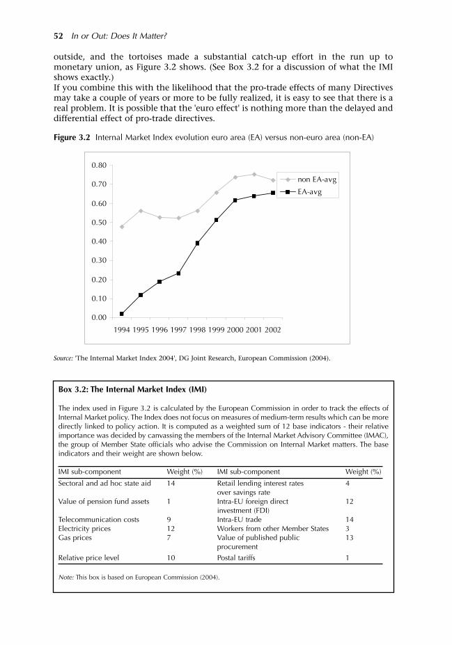
outside, and the tortoises made a substantial catch-up effort in the run up tomonetary union, as Figure 3.2 shows. (See Box 3.2 for a discussion of what the IMIshows exactly.)If you combine this with the likelihood that the pro-trade effects of many Directivesmay take a couple of years or more to be fully realized, it is easy to see that there is areal problem. It is possible that the 'euro effect' is nothing more than the delayed anddifferential effect of pro-trade directives.
52 In or Out: Does It Matter?
0.00
0.10
0.20
0.30
0.40
0.50
0.60
0.70
0.80
1994 1995 1996 1997 1998 1999 2000 2001 2002
non EA-avg
EA-avg
Figure 3.2 Internal Market Index evolution euro area (EA) versus non-euro area (non-EA)
Source: 'The Internal Market Index 2004', DG Joint Research, European Commission (2004).
Box 3.2: The Internal Market Index (IMI)
The index used in Figure 3.2 is calculated by the European Commission in order to track the effects ofInternal Market policy. The Index does not focus on measures of medium-term results which can be moredirectly linked to policy action. It is computed as a weighted sum of 12 base indicators - their relativeimportance was decided by canvassing the members of the Internal Market Advisory Committee (IMAC),the group of Member State officials who advise the Commission on Internal Market matters. The baseindicators and their weight are shown below.
IMI sub-component Weight (%) IMI sub-component Weight (%)
Sectoral and ad hoc state aid 14 Retail lending interest rates 4over savings rate
Value of pension fund assets 1 Intra-EU foreign direct 12investment (FDI)
Telecommunication costs 9 Intra-EU trade 14Electricity prices 12 Workers from other Member States 3Gas prices 7 Value of published public 13
procurement
Relative price level 10 Postal tariffs 1
Note: This box is based on European Commission (2004).

3.6 Bottom line
Here I end my 'Doubting Thomas' digression. All three of the sources for spuriousresults should be taken seriously by empirical researchers, but I believe a Rose effecthappened. Apart from the econometric evidence reviewed above, my belief isbolstered by anecdotal evidence in abundance. Just tell any group of Europeanbusinesspeople especially ones who own small or medium enterprises that theeuro had no impact on trade inside Europe. After a guffaw, you will almost surely hear'of course, it did'. Now it is time to think about the microeconomics of why.
Is the Euro Area Rose Effect a Spurious Result? 53
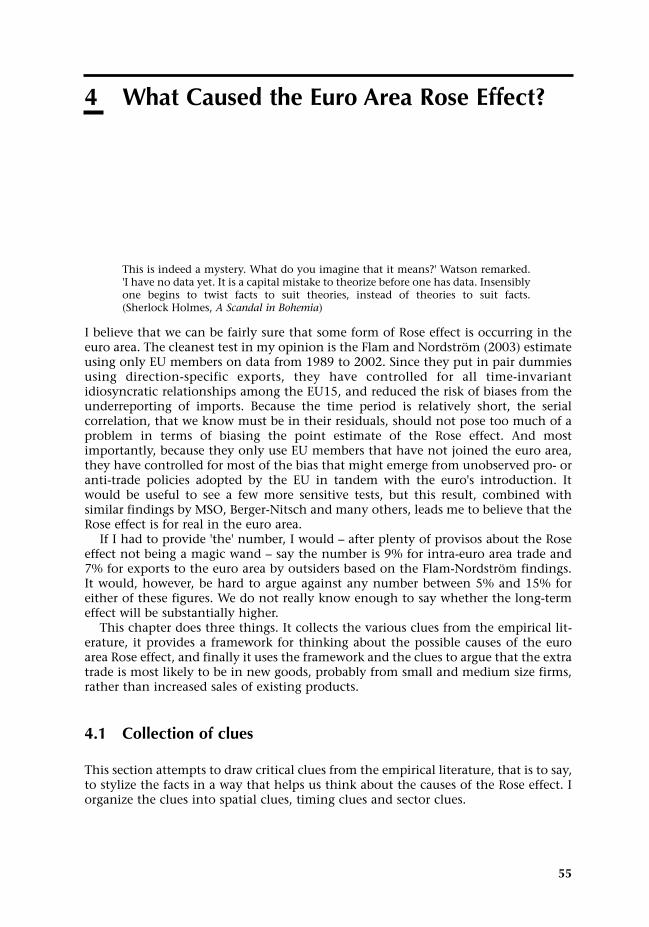
This is indeed a mystery. What do you imagine that it means?' Watson remarked.'I have no data yet. It is a capital mistake to theorize before one has data. Insensiblyone begins to twist facts to suit theories, instead of theories to suit facts. (Sherlock Holmes, A Scandal in Bohemia)
I believe that we can be fairly sure that some form of Rose effect is occurring in theeuro area. The cleanest test in my opinion is the Flam and Nordström (2003) estimateusing only EU members on data from 1989 to 2002. Since they put in pair dummiesusing direction-specific exports, they have controlled for all time-invariantidiosyncratic relationships among the EU15, and reduced the risk of biases from theunderreporting of imports. Because the time period is relatively short, the serialcorrelation, that we know must be in their residuals, should not pose too much of aproblem in terms of biasing the point estimate of the Rose effect. And mostimportantly, because they only use EU members that have not joined the euro area,they have controlled for most of the bias that might emerge from unobserved pro- oranti-trade policies adopted by the EU in tandem with the euro's introduction. Itwould be useful to see a few more sensitive tests, but this result, combined withsimilar findings by MSO, Berger-Nitsch and many others, leads me to believe that theRose effect is for real in the euro area.
If I had to provide 'the' number, I would after plenty of provisos about the Roseeffect not being a magic wand say the number is 9% for intra-euro area trade and7% for exports to the euro area by outsiders based on the Flam-Nordström findings.It would, however, be hard to argue against any number between 5% and 15% foreither of these figures. We do not really know enough to say whether the long-termeffect will be substantially higher.
This chapter does three things. It collects the various clues from the empirical lit-erature, it provides a framework for thinking about the possible causes of the euroarea Rose effect, and finally it uses the framework and the clues to argue that the extratrade is most likely to be in new goods, probably from small and medium size firms,rather than increased sales of existing products.
4.1 Collection of clues
This section attempts to draw critical clues from the empirical literature, that is to say,to stylize the facts in a way that helps us think about the causes of the Rose effect. Iorganize the clues into spatial clues, timing clues and sector clues.
4 What Caused the Euro Area Rose Effect?
55
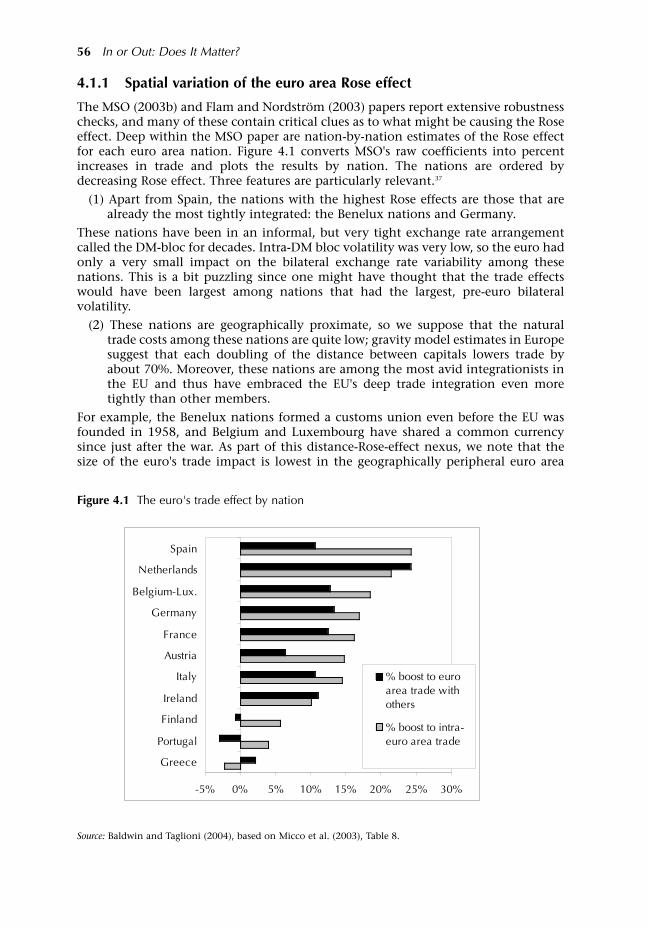
4.1.1 Spatial variation of the euro area Rose effect
The MSO (2003b) and Flam and Nordström (2003) papers report extensive robustnesschecks, and many of these contain critical clues as to what might be causing the Roseeffect. Deep within the MSO paper are nation-by-nation estimates of the Rose effectfor each euro area nation. Figure 4.1 converts MSO's raw coefficients into percentincreases in trade and plots the results by nation. The nations are ordered bydecreasing Rose effect. Three features are particularly relevant.37
(1) Apart from Spain, the nations with the highest Rose effects are those that arealready the most tightly integrated: the Benelux nations and Germany.
These nations have been in an informal, but very tight exchange rate arrangementcalled the DM-bloc for decades. Intra-DM bloc volatility was very low, so the euro hadonly a very small impact on the bilateral exchange rate variability among thesenations. This is a bit puzzling since one might have thought that the trade effectswould have been largest among nations that had the largest, pre-euro bilateralvolatility.
(2) These nations are geographically proximate, so we suppose that the naturaltrade costs among these nations are quite low; gravity model estimates in Europesuggest that each doubling of the distance between capitals lowers trade byabout 70%. Moreover, these nations are among the most avid integrationists inthe EU and thus have embraced the EU's deep trade integration even moretightly than other members.
For example, the Benelux nations formed a customs union even before the EU wasfounded in 1958, and Belgium and Luxembourg have shared a common currencysince just after the war. As part of this distance-Rose-effect nexus, we note that thesize of the euro's trade impact is lowest in the geographically peripheral euro area
56 In or Out: Does It Matter?
-5% 0% 5% 10% 15% 20% 25% 30%
Greece
Portugal
Finland
Ireland
Italy
Austria
France
Germany
Belgium-Lux.
Netherlands
Spain
% boost to euroarea trade withothers
% boost to intra-euro area trade
Figure 4.1 The euro's trade effect by nation
Source: Baldwin and Taglioni (2004), based on Micco et al. (2003), Table 8.

nations: Greece, Portugal, Finland and Ireland. Again this suggests a negativerelationship between trade costs and the Rose effect.
(3) Berger and Nitsch (2005) point out that estimates of the Rose effect on an EUsample that excludes the DM bloc turn out to be insignificant. In other words,the effect is not just strong in these countries, the aggregate numbers like 5% to10% are actually driven entirely by these nations.
The fact can be read in two ways. Pessimistically, it says that it is not the euro, butsome unobserved policy adopted by DM bloc nations that is driving the results. Butwhat could it be: general product and labour market reforms that Britain, Denmarkand Sweden had already undertaken? Optimistically, it could be that exactly becausethese nations had such low exchange rate volatility for so long, their firms were in agood position to profit from the removal of small costs. If this is right, we should seethe Rose effect appearing in the non-DM euro area members, but more slowly.
4.1.2 Trade with non-euro area nations: lack of trade diversion
Intriguingly, MSO (2003b) find that trade between euro area nations and othernations rose with the euro's introduction, but not quite as much. Specifically, theyestimate what might be called a one-sided euro dummy (EMU 1) which value is unityfor any trading pair that involves only one euro area member (the regular eurodummy, or two-sided dummy EMU 2, is only for trading pairs where both nations arein the euro area). The results in their two datasets (one for EU nations only and onethat also includes some European and non-European nations who are not in the EU)are shown in Table 4.1.
What Caused the Euro Area Rose Effect? 57
Table 4.1 Trade diversion results, MSO (2003)
1992-2002 Dev. sample EU
EMU 2 0.126 0.084(0.019)*** (0.030)***
EMU 1 0.086 0.012(0.015)*** (0.030)
Real GDP -0.008 0.048(0.021) (0.030)
Free trade agreement 0.030 -0.044(0.022) (0.053)
EU 0.000 -0.001(0.001) (0.004)
EU trend 1.108 1.071(0.059)*** (0.077)***
Real exchange rate of country 1 -0.220 -0.134(0.045)*** (0.061)**
Real exchange rate of country 2 -0.288 0.367(0.057)*** (0.099)***
EMU 2 impact 0.134 0.088Transformed S.E. (delta method) (0.015)*** (0.029)***EMU 1 impact 0.090 0.012Transformed S.E. (delta method) (0.016)*** (0.029)Observations 2541 1001Within R2 0.46 0.65Pair country dummies Yes YesYear dummies Yes Yes
Notes: Robust standard errors in parentheses. *Significant at 10%; **significant at 5%; ***significant at 1%.
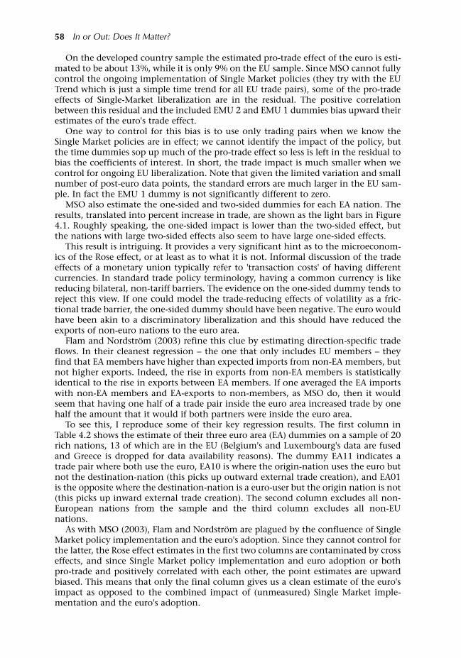
On the developed country sample the estimated pro-trade effect of the euro is esti-mated to be about 13%, while it is only 9% on the EU sample. Since MSO cannot fullycontrol the ongoing implementation of Single Market policies (they try with the EUTrend which is just a simple time trend for all EU trade pairs), some of the pro-tradeeffects of Single-Market liberalization are in the residual. The positive correlationbetween this residual and the included EMU 2 and EMU 1 dummies bias upward theirestimates of the euro's trade effect.
One way to control for this bias is to use only trading pairs when we know theSingle Market policies are in effect; we cannot identify the impact of the policy, butthe time dummies sop up much of the pro-trade effect so less is left in the residual tobias the coefficients of interest. In short, the trade impact is much smaller when wecontrol for ongoing EU liberalization. Note that given the limited variation and smallnumber of post-euro data points, the standard errors are much larger in the EU sam-ple. In fact the EMU 1 dummy is not significantly different to zero.
MSO also estimate the one-sided and two-sided dummies for each EA nation. Theresults, translated into percent increase in trade, are shown as the light bars in Figure4.1. Roughly speaking, the one-sided impact is lower than the two-sided effect, butthe nations with large two-sided effects also seem to have large one-sided effects.
This result is intriguing. It provides a very significant hint as to the microeconom-ics of the Rose effect, or at least as to what it is not. Informal discussion of the tradeeffects of a monetary union typically refer to 'transaction costs' of having differentcurrencies. In standard trade policy terminology, having a common currency is likereducing bilateral, non-tariff barriers. The evidence on the one-sided dummy tends toreject this view. If one could model the trade-reducing effects of volatility as a fric-tional trade barrier, the one-sided dummy should have been negative. The euro wouldhave been akin to a discriminatory liberalization and this should have reduced theexports of non-euro nations to the euro area.
Flam and Nordström (2003) refine this clue by estimating direction-specific tradeflows. In their cleanest regression the one that only includes EU members theyfind that EA members have higher than expected imports from non-EA members, butnot higher exports. Indeed, the rise in exports from non-EA members is statisticallyidentical to the rise in exports between EA members. If one averaged the EA importswith non-EA members and EA-exports to non-members, as MSO do, then it wouldseem that having one half of a trade pair inside the euro area increased trade by onehalf the amount that it would if both partners were inside the euro area.
To see this, I reproduce some of their key regression results. The first column inTable 4.2 shows the estimate of their three euro area (EA) dummies on a sample of 20rich nations, 13 of which are in the EU (Belgium's and Luxembourg's data are fusedand Greece is dropped for data availability reasons). The dummy EA11 indicates atrade pair where both use the euro, EA10 is where the origin-nation uses the euro butnot the destination-nation (this picks up outward external trade creation), and EA01is the opposite where the destination-nation is a euro-user but the origin nation is not(this picks up inward external trade creation). The second column excludes all non-European nations from the sample and the third column excludes all non-EUnations.
As with MSO (2003), Flam and Nordström are plagued by the confluence of SingleMarket policy implementation and the euro's adoption. Since they cannot control forthe latter, the Rose effect estimates in the first two columns are contaminated by crosseffects, and since Single Market policy implementation and euro adoption or bothpro-trade and positively correlated with each other, the point estimates are upwardbiased. This means that only the final column gives us a clean estimate of the euro'simpact as opposed to the combined impact of (unmeasured) Single Market imple-mentation and the euro's adoption.
58 In or Out: Does It Matter?

In the final column the best estimates the intra-EA Rose effect is much smaller,only about 9% (0.088) and the external trade creation is only inward and is equal toabout 7% (0.071). The coefficient for EA exporters to the 'outs' is close to zero (0.8%)and not statistically significant. These are what I consider to be the best estimates ofthe pro-trade effects of the euro. Of course readers can see that the other estimatessuggest that the euro boosted the EA's external exports as much as it boosted its exter-nal imports, but I believe these estimates are biased. Specifically, I believe they assignto the euro dummy an influence that should properly be assigned to (unmeasured)Single Market policies that give EA's exports an edge in non-EU markets.
This is a powerful clue, if it is true. It suggests that the euro has acted more like aunilateral trade liberalization than a preferential trade liberalization. If it is true, italso has some very important implications for the politics of euro area enlargement.I'll have a lot more to say about these in Chapter 5 because it reverses some of theunderpinnings of OCA theory. In basic OCA theory, you have to give up yourmonetary autonomy to get the benefits of reduced transaction costs. If this result isright, it suggests that Britain, Denmark and Sweden were the clever ones from amercantilist perspective they got the better market access without sacrificing theirmain macro-policy tool.
What Caused the Euro Area Rose Effect? 59
Table 4.2 Internal and external trade creation, Flam and Nordström (2003) estimates
All nations Only European nations Only EU nations
EA11 0.139*** 0.114*** 0.088***(0.020) (0.025) (0.025)
EA10 0.077*** 0.064*** 0.008(0.017) (0.023) (0.027)
EA01 0.072*** 0.071*** 0.071***(0.018) (0.024) (0.025)
ln(RYi) 1.222*** 1.214*** 1.194***(0.071) (0.083) (0.080)
ln(RYj) 1.146*** 1.077*** 0.990***(0.069) (0.074) (0.072)
ln(REXRij) -1.058*** -1.119*** -1.292***(0.050) (0.066) (0.063)
ln(REXRcj) 0.722*** 1.026*** 1.024***(0.067) (0.080) (0.083)
nomexr -0.940** -1.257*** -1.460***(0.443) (0.448) (0.448)
eunew 0.013 0.001 -0.002(0.013) (0.013) (0.012)
UR 0.105***(0.018)
obs 4732 2912 2184panels 338 208 156R2 0.99 0.99 0.99
Notes: Robust standard errors in parentheses. *Significant at 10%; **significant at 5%; ***significant at 1%.Year, EU membership, 'Rotterdam effect' and bilateral (fixed effects) dummies included but not reported. RY isreal GDP, REXR are real exchange rates (bilateral and effective), nomexr is a measure of bilateral exchange ratevolatility and eunew picks up the EU membership of Sweden, Finland and Austria; UR is the Uruguay Rounddummy.
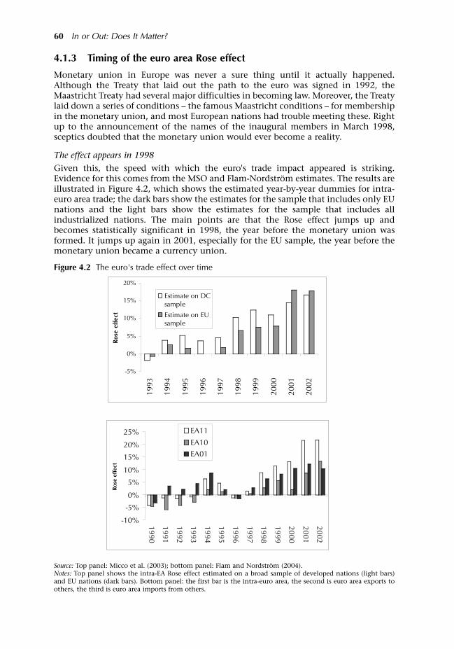
4.1.3 Timing of the euro area Rose effect
Monetary union in Europe was never a sure thing until it actually happened.Although the Treaty that laid out the path to the euro was signed in 1992, theMaastricht Treaty had several major difficulties in becoming law. Moreover, the Treatylaid down a series of conditions the famous Maastricht conditions for membershipin the monetary union, and most European nations had trouble meeting these. Rightup to the announcement of the names of the inaugural members in March 1998,sceptics doubted that the monetary union would ever become a reality.
The effect appears in 1998
Given this, the speed with which the euro's trade impact appeared is striking.Evidence for this comes from the MSO and Flam-Nordström estimates. The results areillustrated in Figure 4.2, which shows the estimated year-by-year dummies for intra-euro area trade; the dark bars show the estimates for the sample that includes only EUnations and the light bars show the estimates for the sample that includes allindustrialized nations. The main points are that the Rose effect jumps up andbecomes statistically significant in 1998, the year before the monetary union wasformed. It jumps up again in 2001, especially for the EU sample, the year before themonetary union became a currency union.
60 In or Out: Does It Matter?
-5%
0%
5%
10%
15%
20%
1993
1994
1995
1996
1997
1998
1999
2000
2001
2002
Ros
e ef
fect
Estimate on DCsample
Estimate on EUsample
-10%
-5%
0%
5%
10%
15%
20%
25%
1990
1991
1992
1993
1994
1995
1996
1997
1998
1999
2000
2001
2002
Ros
e ef
fect
EA11
EA10
EA01
Source: Top panel: Micco et al. (2003); bottom panel: Flam and Nordström (2004).Notes: Top panel shows the intra-EA Rose effect estimated on a broad sample of developed nations (light bars)and EU nations (dark bars). Bottom panel: the first bar is the intra-euro area, the second is euro area exports toothers, the third is euro area imports from others.
Figure 4.2 The euro's trade effect over time

The rapid reaction of trade flows is quite remarkable since the MSO and Flam-Nordström papers control for the main determinants of bilateral trade. The speed alsoprovides us with an important hint as to what is not going on here. Such a rapidincrease in trade would be very hard to explain if, for example, it was driven by theconstruction of new plants related to the unwinding of hedging-related foreign directinvestment.
Sensitivity to the period of estimation
Another clue relates to the nexus between the size of the estimated Rose effect andthe sample period. The original draft MSO sent to Economic Policy six months beforethey presented the paper in Athens used two data samples, one from 1980 to 2002
What Caused the Euro Area Rose Effect? 61
0
5
10
15
20
25
30
1948 1953 1958 1963 1968 1973 1978 1983 1988 1993 1998 2003
EMU11Europemin/max
0
10
20
30
40
50
60
70
80
90
100
1957
1958
1959
1960
1961
1962
1963
1964
1965
1966
1967
1968
1969
1970
1971
1972
1973
1974
1975
1976
1977
1978
1979
1980
1981
1982
1983
1984
1985
1986
1987
1988
1989
1990
1991
1992
1993
1994
1995
1996
1997
1998
1999
2000
2001
Customs Union (1968)
Monetary Union (1999)
Common Market (1993)
EMS (1979)
CAP (1962)
Source: Top panel: Berger and Nitsch (2005); bottom panel: Mongelli et al. (2005).
Figure 4.3 Indices of European integration over time

and one from 1992 to 2002. Although the regressions have some serious problemsthat may vitiate the results, the early MSO seems to find that the Rose effect is biggerwhen a longer dataset is used. Berger and Nitsch (2005) confirm this result when theyextend the period back to 1948 and push it forward one more year to include 2003. The finding that the Rose effect was bigger for samples starting further back is highlysuspicious. It suggests that the various dummies for EU integration are not reallyremoving everything but the euro from the data. Figure 4.3 shows that Europeaneconomic integration has been an ongoing process for the last 50 years. The top panelis from Berger and Nitsch (2005) and the bottom panel is from Mongelli et al. (2005).Both show that economic integration was rising steeply just before the introductionof the euro. If pro-trade adjustments to pre-euro area integration take time, it couldvery well be that the lagged effects of Single Market measures are showing up in thepost-1999 data and being confused with the trade effects of the euro.
At the heart of this suspicion is a mis-specification of the lags and the role ofEuropean integration. In principle this is testable and correctable with proper econo-metrics. For example, Flam and Nordström (2003) allow for a time-varying EUdummy and they find that their Rose effect estimate is affected very little by a changein their sample period. In any case, the diagram showing the Flam-Nordström resultsfor the EA dummy and EU dummy suggests that it may be quite difficult to tease apartthe effects of general European integration and the euro per se. Indeed, Berger andNitsch (2005) go so far as to argue that since a time trend for integration among theeuro area members wipes out the Rose effect, the MSO estimates are due to a mis-spec-ification.
62 In or Out: Does It Matter?
Table 4.3 Rose effect and volatility impact by sector
isic Industry Rose t-stat Volatility t-stateffect
40-41 electricity, gas and water supply 1.64 4.47 -15.78 -1.87351 building and repairing of ships and boats 0.57 2.00 -15.87 -2.4215-16 food products, beverages and tobacco 0.40 2.64 -7.78 -2.2325 rubber and plastics products 0.35 2.25 -10.73 -3.0435 other transport equipment 0.34 1.84 -17.72 -4.2330 office, accounting and computing machinery 0.32 1.91 -5.77 -1.5034 motor vehicles, trailers and semi-trailers 0.31 1.81 -13.78 -3.5332 radio, television and communication equipment 0.27 1.68 -14.06 -3.7436-37 manufacturing n.e.c.; recycling 0.27 1.76 -6.25 -1.76353 aircraft and spacecraft 0.27 1.09 -16.89 -2.9833 medical, precision and optical instruments 0.27 1.76 -7.75 -2.2231 electrical machinery and apparatus, n.e.c. 0.26 1.64 -14.13 -3.9428 fabricated metal products 0.25 1.66 -9.78 -2.8517-19 textiles, textile products, leather and footwear 0.25 1.54 -12.00 -3.2524 hemicals and chemical products 0.25 1.52 -8.80 -2.3820 wood and products of wood and cork 0.23 1.41 -7.78 -2.0829 machinery and equipment, n.e.c. 0.23 1.44 -9.29 -2.5427 basic metals 0.19 1.16 -14.23 -3.7026 other non-metallic mineral products 0.19 1.24 -10.29 -2.91271+2731 iron and steel 0.14 0.74 -13.25 -3.082423 pharmaceuticals 0.13 0.70 -8.04 -1.90272+2732 non-ferrous metals 0.12 0.63 -20.52 -4.7201-05 agriculture, hunting, forestry and fishing 0.09 0.50 -7.59 -1.9123 coke, refined petroleum products + nuclear fuel 0.03 0.12 -7.83 -1.33352+359 railroad equipment + transport equipment n.e.c. -0.05 -0.23 -14.09 -2.9610-14 mining and quarrying -0.21 -1.15 -9.84 -2.37
Source: Adapted from Baldwin et al. (2003).
4.1.4 Sectoral variation in the euro area Rose effect
While most studies of the euro's impact have focused on aggregate trade data,Taglioni (2002) and Baldwin et al. (2005) run the standard gravity model usingsectoral data. In addition to confirming the general findings of the aggregate studieswhen all the sectors are pooled, this paper also provides sector-specific estimates ofthe Rose effect. The results are shown in Table 4.3.What these results show is a rough correlation between the size of the Rose effect andwhat we loosely call ICIR sectors (imperfect competition and increasing returnsectors). At the bottom of the list, we have agriculture as well as mining andquarrying, while near the top, we have various types of machinery and highlydifferentiated consumer goods such as food products, beverages and tobacco. Thisfinding opens the door to the possibility that ICIR like effects for example, theimpact of uncertainty on market structure may be part of the story.
The Flam-Nordström paper also provides sector results, which are reproduced inTable 4.4. These are broadly in line with the earlier estimates in Table 4.3. The sectorswithout a Rose effect tend to be those marked by fairly homogeneous products. Recallthat trade inside Europe in agricultural goods is not free trade. Although there are noformal barriers, market intervention is pervasive.
As should be expected given the large number of studies reviewed, the collectionof clues is far from cohesive. I turn now to introducing a framework that helps organ-ize thinking on the causes of the Rose effect in the euro area.
4.2 Microeconomic changes that could produce a Rose effect
With the clues in hand it is time to twists the theories to fit the facts. By my count, there are two channels through which the euro could have affected
trade flows. I base this assertion on an uncontroversial theory, namely the demandfunction. Taking the destination nation's CES demand function for goods from theorigin nation (nation-o):
Since we have fairly good data on real expenditure, the structural break in thisdemand equation i.e. the Rose effect must be coming through one of twochannels:
A change in the unobservable number-of-varieties variable.
A change in the relative price that is not captured by the data included in theregressions.38
The relative price channel
The relative price has a numerator and a denominator. The numerator is the price ofa typical nation-o variety in nation-d. The denominator is a price index of allcompeting varieties in nation-d's market. As usual, we will measure all prices in thenumeraire which we take here to be dollars.
What Caused the Euro Area Rose Effect? 63
×
=
−
eexpenditur
realsd'Nation
dnation in
varietiesonation
ofpriceRelative
dnation to
exported varieties
onationofNumber
dtoonation
fromExportselasticity
demandimport
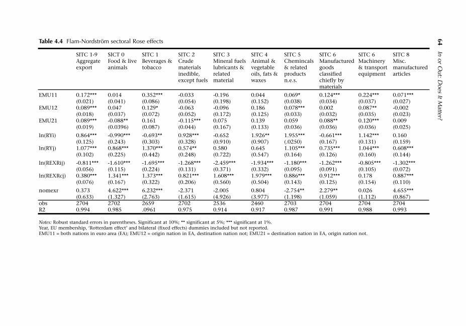
64In or O
ut: Does It M
atter?
Table 4.4 Flam-Nordström sectoral Rose effects
SITC 1-9 SICT 0 SITC 1 SITC 2 SITC 3 SITC 4 SITC 5 SITC 6 SITC 6 SITC 8Aggregate Food & live Beverages & Crude Mineral fuels Animal & Chemincals Manufactured Machinery Misc.export animals tobacco materials lubricants & vegetable & related goods & transport manufactured
inedible, related oils, fats & products classified equipment articlesexcept fuels material waxes n.e.s. chiefly by
materials
EMU11 0.172*** 0.014 0.352*** -0.033 -0.196 0.044 0.069* 0.124*** 0.224*** 0.071***(0.021) (0.041) (0.086) (0.054) (0.198) (0.152) (0.038) (0.034) (0.037) (0.027)
EMU12 0.089*** 0.047 0.129* -0.063 -0.096 0.186 0.078*** 0.002 0.087** -0.002(0.018) (0.037) (0.072) (0.052) (0.172) (0.125) (0.033) (0.032) (0.035) (0.023)
EMU21 0.089*** -0.088** 0.161 -0.115*** 0.075 0.139 0.059 0.088** 0.120*** 0.009(0.019) (0.0396) (0.087) (0.044) (0.167) (0.133) (0.036) (0.036) (0.036) (0.025)
ln(RYi) 0.864*** -0.990*** -0.693** 0.928*** -0.652 1.926** 1.955*** -0.661*** 1.142*** 0.160(0.125) (0.243) (0.303) (0.328) (0.910) (0.907) (.0250) (0.167) (0.131) (0.159)
ln(RYj) 1.077*** 0.868*** 1.370*** 0.574** 0.580 0.645 1.105*** 0.735*** 1.044*** 0.608***(0.102) (0.225) (0.442) (0.248) (0.722) (0.547) (0.164) (0.126) (0.160) (0.144)
ln(REXRij) -0.811*** -1.610*** -1.695*** -1.268*** -2.459*** -1.934*** -1.180*** -1.262*** -0.805*** -1.302***(0.056) (0.115) (0.224) (0.131) (0.371) (0.332) (0.095) (0.091) (0.105) (0.072)
ln(REXRcj) 0.380*** 1.341*** 1.373*** 0.821*** 1.608*** 1.979*** 0.886*** 0.912*** 0.178 0.887***(0.076) (0.167) (0.322) (0.206) (0.560) (0.504) (0.143) (0.125) (0.154) (0.110)
nomexr 0.373 4.622*** 6.232*** -2.371 -2.005 0.804 -2.754** 2.279** 0.026 4.655***(0.633) (1.327) (2.763) (1.615) (4.926) (3.977) (1.198) (1.059) (1.112) (0.867)
obs 2704 2702 2659 2702 2536 2460 2703 2704 2704 2704R2 0.994 0.985 .0961 0.975 0.914 0.917 0.987 0.991 0.988 0.993
Notes: Robust standard errors in parentheses. Significant at 10%; ** significant at 5%; *** significant at 1%.Year, EU membership, Rotterdam effect and bilateral (fixed effects) dummies included but not reported.EMU11 = both nations in euro area (EA); EMU12 = origin nation in EA, destination nation not; EMU21 = destination nation in EA, origin nation not.

Turning first to the numerator, the price is related to the three terms in parenthe-ses below, i.e. the bilateral mark-up, µod, the bilateral trade costs, τod, and nation-o'smarginal production costs measured in dollars, µco. In symbols:
This is true by definition, taking µ to be exactly the ratio of pod to the domesticmarginal production costs plus the bilateral trade costs.
The CES price index of all competing varieties will be the geometric average of theprice of all competing varieties sold in nation-d, including those made in nation-d.That is:
The new varieties channel
Many varieties in nation-o are not exported to nation-d, a fact that has now beenextensively documented in the so-called new-new trade theory (see Bernard et al.,2000). Notice that the n's enter the denominator of the relative price term, so the twochannels are not mutually exclusive although a change in nod will have a first-orderlarge impact on bilateral trade, while changes in nation-i's nid will affect o-to-d tradeflows only indirectly.39 In what follows, we turn to these channels one by one,considering the testable implications of each.
4.2.1 The relative price channel
Given the pass-through relationship and the definition of relative price, there arethree ways in which the relative price channel could operate: a change in transactioncosts (as measured by τ), a change in the mark-up (as measured by µ), or a change inthe price index Pd. We consider each of these in turn and explain why each isinconsistent with the collection of clues summarized above.
Bilateral transaction costs: the Mundell story
In the traditional optimal currency area story, two nations that share the same moneyface lower transaction costs on bilateral trade and therefore trade more with eachother. This is certainly the model that most Rose-effect researchers seem to have inthe back of their minds when running their regressions.
I believe that the evidence completely rejects the standard transaction costs storyand this on three separate counts. To make the case, we need to take the story seri-ously and work out what the theory tells us must be true in the data if the transac-tion cost story is right.
Implied transaction cost changesSuppose the Rose effect on intra euro area is 10%. What would the reduction inbilateral transaction cost have to be if it was the main, indeed, the only changeresponsible for the Rose effect? The answer depends upon two elasticities and a share:the pass-through elasticity that determines what fraction of the transaction costsavings is passed on to consumers in the export market, the import demand elasticityin the importing nation, and the share of a euro area nation's expenditure that isaffected by the changes. Totally differentiating the demand equation, we get:
What Caused the Euro Area Rose Effect? 65
))()(( oododod mcp τµ=
∑ −=i idididd mcnP στµ 1)(
dodod PpX ˆ)1()ˆ(ˆ −+−= σσ (3)
Here the '^' symbol means proportional change. Under the maintained hypothesisthat lower intra-EA transaction costs are the culprit, the bilateral τ should fall for allof nation-d's partners in the EA. This means that the price index change will be larger,the large is nation-d's share of expenditure on imports from the euro area. The preciseformula is:
where shareEA is share of expenditure in a typical EA member that falls on importsfrom other EA members. Leaning heavily on the assumption that transaction costsare driving the whole Rose effect, we see that the proportional change in the price willbe the proportional change in the τ. The actual connection between the change intransaction costs and the landed price of imports will depend upon how much of thetransaction cost reduction are passed on to foreign customers. Specifically,
where PT stands for 'pass through'. Empirically, the pass-though elasticity forexchange rate changes is much less than unity (Goldberg and Knetter, 1997), butthere is an argument that a once-and-forever change in transaction cost would bepassed through more fully. Combining all the steps, we get the implied connectionbetween the transaction cost reduction and the trade volume change. It is:
There are rough estimates as to the size of the transaction cost saving , for exampleEuropean Commission (1990) puts it at 0.5% of GDP, but these are extremely crudeand surely underestimate the total costs. Rather than trying to gauge the averagesavings, we reverse the deduction. We take 10% trade creation as data and ask howbig the euro-induced drop transaction costs must have been to account for it.
To get an idea of what sort of transaction cost savings would be necessary, Table 4.5solves for percent change in t that is implied by a 10% Rose effect under variousassumptions on the demand elasticity (σ), the expenditure share and the pass-through elasticity. The left panel assumes full pass-through (of the transaction costsavings to trade prices) and then considers various combinations of import demandelasticities (down the leftmost column, ranging from 8 to 1) and EA-import expendi-ture shares (across the top of the panel, ranging from 0.5 to 0.1). For example, if theelasticity is very high at 8 and the import share is very low at 0.1, then the impliedchange in τ is only 1%. It is clear that the import demand elasticity is by far the mostimportant parameter.
There is some dispute as to the true value of the import demand elasticity. At oneextreme, Obstfeld and Rogoff (2000) assume, without empirical justification, that itis 8. Most empirical estimates yield an elasticity that is substantially lower. Gagnon(2003), for example, say his 'price elasticities for the most part are estimated close to-1, which is typical for the literature'. Elasticities above 4 are considered to be veryhigh.
Taking a middle of the road estimate for the elasticity, say 2, and a 40% EA-importsexpenditure share, the implied transaction cost reduction would have to be 6%. Ifthere is less than full pass-through, the number has to be even higher.
It is important to note that this 6% transaction cost savings has to be on margin-al costs, not average costs, since only marginal cost changes could get passed throughto prices in the short run. Moreover, since the Rose effect seems to have appeared
66 In or Out: Does It Matter?
)ˆ(ˆodEZd pshareP =
odod elasticityPTp τ)(ˆ =
( ) odEZEZod elasticityPTshareshareX τσ ˆ)()1(ˆ −−=

immediately, the transaction cost savings would have to be immediate, if it is the cul-prit. What sort of transaction costs could we be talking about? In the Mundellian tra-dition, the nature of these costs is usually left vague, but presumably they involve for-eign exchange market commissions and some additional administrative costs forfirms.
Problems with the bilateral transaction cost storyI believe there are three problems with transaction-cost savings of this magnitude.
First, I find it hard to believe that corporations in Europe faced a marginal costof 6% when switching between major European currencies. This admittedly isbased on my priors and readers may or may not share them. The next twoobjections, however, are more scientific.
Second, if transaction costs fell 6%, we should have seen a Rose effect in mostsectors. Of course, since demand elasticities vary widely by sector, we canunderstand that there was some variation across sectors, but the Flam-Nordström and Baldwin-Taglioni results suggest that impact was concentrated ina few sectors. Flam-Nordström, for example, find a positive and statisticallysignificant Rose effect in only four of the nine main categories of trade (SITCcategories 0 to 8), and in two of the remaining five categories the effect isestimated as negative although not statistically significant.
Third, the Rose effect appeared very quickly, in 1999 or even a year earlier,according to most studies. If the Mundellian story was responsible for this, the6% transaction cost drop would have had to have been passed through to euroarea trade prices quickly. This, in turn, means that we should have observed astructural break in the trade pricing equations and a sizeable one-off jump ineuro area price convergence. As the literature reviewed in Chapter 2 showed, itappears that there has been some slow convergence, but definitely no jump inprice convergence. Since such a price convergence jump is exactly what thetransaction cost story asserts is behind the Rose effect, the failure to observesuch a jump tells us that transactions costs were not the culprit, at least not inthe early years of the monetary union.
What Caused the Euro Area Rose Effect? 67
Table 4.5 Transaction cost drop (%) implied by a 10% Rose effect, various elasticities and shares
Pass-through Pass-throughelasticity 1.0 elasticity 0.5
EA importsexpenditure share: 0.5 0.4 0.2 0.1 0.5 0.4 0.2 0.1
Import demandelasticity: 8 -2 -2 -2 -1 -4 -4 -3 -35 -3 -3 -2 -2 -7 -6 -5 -43 -5 -5 -4 -4 -10 -9 -8 -72 -7 -6 -6 -5 -13 -13 -11 -111 -10 -10 -10 -10 -20 -20 -20 -20
Source: Author's calculations. Note: Percent figures rounded off by excel to the nearest 1%. The formula is: dτ/t = (Rose effect)/(-σ + (σ-1)S) ´PTelas, where S is the EA share and PTelas is the pass-through elasticity.

Pricing transparency and the intra-EA mark-up
Pricing transparency is, after transaction costs, the most frequent hand-wavingargument made for why we should believe that the euro could stimulate trade. Thepoint is mentioned in the 1970 Werner report and echoed in the Commission's 1990'One Market, One Money' report where the European Commission argued that'without a completely transparent and sure rule of the law of one price for tradablegoods and services, which only a single currency can provide, the single marketcannot be expected to yield its full benefits static and dynamic'. The Commissionrestated the argument in its 1996 Single Market Review, claiming 'increased pricetransparency will enhance competition and whet consumer appetites for foreigngoods; price discrimination between different national markets (in the EU) will bereduced'. Translating their words into my organizing framework (the demandequation), the argument is that participation in the euro area could change the mark-up m in the above expressions.
A good way of thinking about the mark-up is as a measure of the degree of com-petition. The basic notion is that the euro promotes competition, which depressesprice-cost mark-ups thus making imports cheaper. The net result is an increase in euroarea imports. Since we do not have good data on the mark-ups, this sort of changewould show up as a structural break in the gravity equation that is associated withusage of the euro (i.e. as a Rose effect).
Merits of the mark-up storyThe mark-up change (implicitly due to a price-transparency-induced rise incompetition) has many advantages over the transaction cost story.
The notion turns on a change in the markets of euro area nations changes thatmake them extra good at importing (since import prices are depressed) without nec-essarily making them extra good at exporting. This means that the story is consistentwith the 'clue' that the euro leads to no trade diversion.
Furthermore, the mark-up hypothesis is sufficiently flexible to account for thenational and sector diversity in the Rose effect estimates. One could expect that theeuro would increase competition among euro area companies, and indeed this iswhat many trade practitioners will tell you. However, it is quite likely that the effectwould interact in a complex manner with various nation-specific and sector-specificfeatures. For example, if the euro leads to greater price transparency for big-ticketitems like cars and trucks, the impact would be very different in, say, Greece than itwould be in Germany. The two nations differ greatly in terms of local producers andgeographic distance to alternative suppliers. Likewise, the extent of the change in themark-up could easily vary by sector. The obvious point is that the mark-up is prettysmall already in some sectors and so unlikely to fall further. The more subtle point isthat the pro-competitive effects of the euro could interact in complex ways withnational regulations; a good example is banking. One would have thought that theelimination of currency risk would have allowed German homebuilders to get a mort-gage in Luxembourg, but domestic regulations and practices effectively prevent thisfor now.
Problems with the mark-up storyThe problem with the mark-up story stems for a feature it shares with the transaction-cost story it implies a sudden convergence in euro area prices as the gap betweenlocal and export prices narrows. Moreover, if the mark-up is really the culprit, thenthe price convergence would have to be sudden and large since it has to account fora 10% increase in trade in the first years of monetary union. This, however, isinconsistent with one of the clues we discussed above, namely there does not seem
68 In or Out: Does It Matter?
to have been a sudden change in price dispersion. This is why I believe we can safelyreject the pricing transparency story as the main culprit. Of course, many things inEurope changed at the same time and this 'crime' is unlikely to have a sole culprit,but we can say that the price transparency story could not have been a major causesince it does not fit with the pricing clues.
The price index route
The only possibility left in the relative price channel is a change in the importingnation's price index of competition goods. This route was discussed in a roundaboutway by Micco et al. (2003b) and explicitly by Flam and Nordström (2003). Thoseauthors noted that the euro's sharp depreciation would lower the price of intra-euroarea trade (measured in dollars) relative to the price of competing goods from thedollar-zone. Since most versions of the gravity model do not explicitly control forexchange rates, such changes would show up as a structural break associated with theuse of the use of the euro, i.e. as a Rose effect.
There are two problems with this story. First, Flam and Nordström (2003) do try tocontrol for exchange rate changes and yet they still find a structural break that isroughly the size of the one found by other authors who do not control for exchangerates (or more precisely they control for bilateral exchanges by averaging the two uni-directional flows between each pair of nations). Second, the basic story requires theexports of non-EA nations to be extraordinarily expensive and thus extraordinarilylow. This conflicts with the clue that non-EA nations seem to have experienced a pos-itive Rose effect, i.e. the euro seems to have resulted in extraordinarily high exportsfrom non-EA members. Indeed, in the Flam-Nordström results that include the USAand Japan, the increase in non-EA exports to the EA due to the euro's introduction iseven larger.
This leads me to reject the price index route as the main suspect. With this routeeliminated, we have eliminated all possible routes in the relative price channel.
4.2.2 New goods – the extensive margin story
Holmes to Watson: 'How often have I said to you that when you have eliminatedthe impossible, whatever remains, however impossible, must be the truth?'(The Sign of Four)
A fascinating paper by Andrew Bernard and Brad Jensen decomposes the growth ofUS exports in the 1990s into an intensive margin, i.e. an increase in the volume ofgoods that were already exported, and an extensive margin, i.e. an increase due tonewly exported goods. The paper, Bernard and Jensen (2004), used data fromindividual plants for the entire US manufacturing to establish this breakdown. Thereally new finding was that a non-negligible share came from firms that switchedbetween only selling locally to selling locally and abroad. This brought to centre stagethe little known fact that most firms in most nations do not export even when theyare in so-called traded goods sectors; they produce only for the local market, oftenselling to other firms.
The relevance of this work here is to alert us to the fact that the Rose effect mighthave happened due to a change in the number of varieties each nation exports. Thereare many things to recommend this idea.
First, since it involves existing firms selling existing varieties in new markets, itcould happen quite quickly.
What Caused the Euro Area Rose Effect? 69
Second, the size of the effect could vary quite a lot across sectors since marketstructures vary so much. For example, the Flam-Nordström results suggest thatthe Rose effect was systematically large in sectors such as chemicals andtransport equipment where scale economies and imperfect competition areimportant, but the effect was small in other sectors.
Third, the size of the effect could vary a great deal across euro area nations sincethe decision to introduce new varieties is constrained by all sorts of legal barriersand implicit market arrangements.
Fourth, the effect could happen without any convergence in prices. Indeed, allthe explanations that work via the relative price term should have also shownup as structural breaks in the pricing equation. But even the most casual glanceat the demand reveals that the number of exported varieties does not enter thepricing equation. A 'structural break' in 'n' would thus create a structural breakin the trade volume equation without creating one in the trade price equation.
Fifth, it could happen without generating trade diversion, if euro usage implieda lower cost of entry into euro area markets.
Melitz model and newly exported goods
Until very recently, mainstream international economics ignored the fact that tradebarriers could affect the number of goods one nation exports to another. Oneinfluential paper that has helped change this is Melitz (2003). The model has muchin common with early trade models such as those by Paul Krugman and ElhananHelpman (1985), but there are two key innovations that add complexity in both thegood and bad sense of the word. Since I believe that the introduction of new goodsis the key to explaining the Rose effect in Europe, it is worth spending some spacedeveloping intuition for these models, the so-called new-new trade theory. We start,however, with its precedent the new trade theory.
Determination of the number of goods produced in the 'new' trade theory The two new elements in the new-new trade theory are: (1) fixed cost of entering anew market; and (2) differences in firm's marginal production costs. These arecombined with the standard elements of the Helpman-Krugman trade model, whichis often called the new trade theory although it is more than 25 years old. To fix ideas,we work out the determination of the number of goods without the two extraelements.
In the new trade theory, firms produced differentiated varieties that compete indi-rectly with each other via monopolistic competition. That is to say, each firm makesa unique variety and it has a monopoly on this, but its market power is limited to theresidual demand curve, namely the demand that is left over after other firms havesold their goods. Firms face increasing returns to scale, so they must sell at least agiven amount to cover costs. Due to this breakeven constraint, the number of firmsis determined in the market; however, in the new trade theory the number of vari-eties a given nation produces is fixed by the nation's supply of productive factors. Bignations (i.e. nations with lots of productive factors) will produce a wider range ofgoods than small nations.
A very insightful way of thinking about the determination of the number of goodsproduced is to think of firms entering until the residual demand curve facing a typi-cal firm has been driven down (or back) to the point where all firms just break even.This is illustrated in Figure 4.4.
In the model of imperfect competition used most frequently in the new trade the-
70 In or Out: Does It Matter?
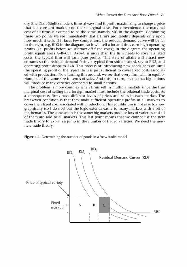
ory (the Dixit-Stiglitz model), firms always find it profit-maximizing to charge a pricethat is a constant mark-up on their marginal costs. For convenience, the marginalcost of all firms is assumed to be the same, namely MC in the diagram. Combiningthese two points we see immediately that a firm's profitability depends only uponhow much it sells. If it faces few competitors, the residual demand curve will be farto the right, e.g. RD3 in the diagram, so it will sell a lot and thus earn high operatingprofits (i.e. profits before we subtract off fixed costs); in the diagram the operatingprofit equals areas A+B+C. If A+B+C is more than the firm needs to cover its fixedcosts, the typical firm will earn pure profits. This state of affairs will attract newentrants so the residual demand facing a typical firm shifts inward, say to RD2, andoperating profit drops to A+B. This process of introducing new goods goes on untilthe operating profit of the typical firm is just sufficient to cover fixed costs associat-ed with production. Now turning this around, we see that every firm will, in equilib-rium, be of the same size in terms of sales. And this, in turn, means that big nationswill produce many varieties compared to small nations.
The problem is more complex when firms sell in multiple markets since the truemarginal cost of selling in a foreign market must include the bilateral trade costs. Asa consequence, firms have different levels of prices and sales in each market. Thebreakeven condition is that they make sufficient operating profits in all markets tocover their fixed cost associated with production. This equilibrium is not easy to showgraphically (so I do not) but the logic extends easily to many markets with a bit ofmathematics. The conclusion is the same; big markets produce lots of varieties and allof them are sold to all markets. This last point means that we cannot use the newtrade theory to explain a jump in the number of traded varieties. We need the new-new trade theory.
What Caused the Euro Area Rose Effect? 71
MC
Residual Demand Curves (RD)
Fixed markup
Price of typical variety
RD2RD3
RD1
A B C
Figure 4.4 Determining the number of goods in a 'new trade' model

Determination of the number of goods produced in the 'new-new' trade theory The new-new trade theory focuses on heterogeneous firms, in particular ondifferences in firm-level efficiency and therefore firm-level marginal costs. To see howthis changes things, consider a diagram similar to Figure 4.4 but where firms havedifferent marginal costs.
To keep things simple, we assume that all varieties are viewed as equally good byconsumers, so they all face the same residual demand function. The heterogeneityonly comes through marginal costs. Starting with a given residual demand curve, wecan show how operating profits vary for firms with different marginal costs in Figure4.5.
The diagram shows three firms with progressively higher marginal costs, MC1, MC2
and MC3. Following the profit-maximizing fixed mark-up pricing rule, the firmscharge progressively higher prices and thus sell progressively less; the small firm (asmeasured by sales) is the high marginal-cost firm. We also see that they earn pro-gressively lower operating profits: areas A, B and C.
In a closed economy this sort of reasoning will give us a 'threshold MC' firms withmarginal costs above some threshold will not find it worthwhile to produce. Thisconcept is quite intuitive and indeed it will suffice for extrapolating to the open econ-omy case that we are really interested in, but it is important to note that this glossesover the major technical difficulties of the Melitz model the position of the resid-ual demand curve. In fact, the residual demand depends upon the number of activefirms (for the reasons discussed in Figure 4.4) and upon the distribution of their mar-ginal costs (if many firms have low marginal costs, they will sell a lot and then theresidual demand curve will be shifted inwards a lot). Thus we must simultaneouslysolve for the number of firms and the threshold marginal cost. This is the source ofmost of the Melitz model's mathematical difficulties. Fortunately, the basic intuitionwe get from a fixed RD curve goes through even with more complete reasoning if weassume that the RD in Figure 4.5 is in its equilibrium position.
72 In or Out: Does It Matter?
Residual Demand Curve (RD)
Price of variety 1
A
B
C
MC2
MC3
MC1
Fixed markup
Fixed markup
Fixed markup
Figure 4.5 Determining the range of goods in a 'new new’ trade model
With all this background firmly in hand, the basic economic logic of thedetermination of the number of traded goods is simple to portray. The key questionis: 'If a firm is already covering its fixed production costs in its local market, will italso export its goods to all other nations in the world?'To address this question, we have to be specific about what separates the local andexport markets, i.e. trade costs. It is natural to suppose that there are per-unit tradecosts the usual costs related to distance and manmade trade barrier that raise thecost by, say, 10% per unit shipped. (In the discussion of the gravity model, I denotedthe marginal trade costs as t.) As mentioned above, a key extra assumption in theMelitz model is that firms face a fixed cost per market. For example, to sell in a newmarket, a firm has to invest something in establishing the brand name (if it is aconsumer product), or establishing contacts with purchasers (if it is an intermediateproduct). There are also fixed costs related to product regulations. Most relevant tothe case at hand is the fixed costs of managing an extra currency; these could involvebank charges, additional staff, more complex accounting procedures, etc.
Using the Figure 4.5 reasoning as an analogy, it is clear that only firms with suffi-ciently low marginal costs will be able to sell to foreign markets, since only they willbe able to cover the fixed market-entry costs (due to the fixed mark-up rule, they fullypass on the per-unit trade costs to foreign customers so the price of their good will behigher in foreign markets). In other words, we will get a second threshold the exportthreshold that determines which domestically produced goods are exported.
This threshold implies that the model's predictions are in line with the commonobservation that big, efficient firms are more likely to export than small firms.Moreover, the further away is the market, the higher will be the price (due to passed-through trade costs) and so the lower will be the operating profit earned. This meansthat firms with a given marginal cost may find it worth their while to pay market-entry costs in nearby markets, but not in distant markets. In other words, the exportthreshold for marginal costs is lower for more distant markets.
The final step is to connect the export threshold and the number of goods export-ed. As the threshold marginal cost rises, smaller firms will export their goods, so therange of exported goods will widen. For completeness sake, note that with twonations the model is analytically solvable but with more nations it can be worked outwith paper and pencil only under highly restrictive assumptions. It can be solvednumerically for general cases, and indeed Rocha (2006) shows that lower one nation'smarket-entry cost can lead to a Rose effect without trade diversion.
The euro's impactFinally, we are ready for the heart of the matter the impact of introducing the euroon the number of goods exported. Assume that the introduction of the euro lowersthe fixed market entry costs in euro area nations. One very concrete story would bethat the fixed costs associated with managing an extra currency are lower for theeuro, which has a large, deep market, than it was for the legacy currencies.Importantly, the assumption is that the fixed cost falls for all exporters to the euroarea, not just for firms that are located inside the euro area. For example, a Swedishfirm that wanted to sell to all 12 euro area nations had to deal with 11 currenciesbefore 1999 (Belgium and Luxembourg have had a currency union since the 1950s),but afterwards it had to deal with only one. Under this story, it is plausible that thedrop in fixed cost would be greater for EA-based firms than for non-EA-based firms.For firms located inside the euro area, all fixed costs related to foreign exchange inthe euro area disappear since after 1999 the local and export currencies are the same.
If the fixed cost of entering the euro area markets falls, then a wider range of firmswill find selling to the euro area to be worthwhile. As a consequence, the number of
What Caused the Euro Area Rose Effect? 73

goods exported to the euro area will increase, both from the euro area nations andfrom non-euro area nations. More goods, in turn, mean a higher trade volume. Notethat this simultaneously accounts for the positive Rose effect within the euro area andthe lack of trade diversion.
Note that this story is flexible enough to account for sector variation and nation-specific variation. In particular, the Melitz model works in industries marked byimperfect competition and increasing returns, but not in commodity-like sectors just the pattern that the sector studies suggest. The key difference is that in com-modity-like sectors, say 'Food and live animals', or 'Crude materials', the market struc-ture is not dominated by individual firms selling differentiated goods. Moreover, evenamong differentiated-goods sectors, the distribution of firm-size can alter the indus-try's response to a given change in the fixed costs. Observe that it is also flexibleenough to allow for geographic variation if one supposes that foreign-exchange-linked market entry costs were affected in different ways in different euro area mem-bers, and that the firm-size distribution is different in different nations.
As far as I know, there are only two formal model of the new goods hypothesis.Baldwin and Taglioni (2004) present a formal model of the Rose effect of this whichhas the additional element of exchange rate uncertainty. The basic intuition is sim-ple. Most European firms are not engaged in trade; they sell only in their local mar-kets due to a variety of reasons one of which is aversion to exchange rate uncer-tainty. Such uncertainty is a nuisance to giant companies like Nestlé and Fiat, but tosmall and medium firms it is a very real barrier. The story is that monetary unioneliminated this uncertainty and thus increased the number of firms in the euro areathat are engaged in exporting to other euro area markets. A sudden and permanentreduction of bilateral volatility within the euro area thus led to an increase in exportswith little change in the basic production structure. This story rests on the Melitzmodel (Melitz, 2003) where the range of firms that export is endogenously deter-mined and related to native firm-level productivity so that large firms export whilesmall firms do not. Rocha (2006) is the other formal model; it focuses on the three-country case and thus can account for the lack of trade diversion (Baldwin-Taglioniworks with only two nations ).
Do the facts fit?
Inspector Gregory: Is there any other point to which you would wish to drawmy attention?Holmes: 'To the curious incident of the dog in the night-time''The dog did nothing in the night time''That was the curious incident, remarked Sherlock Holmes. (from The Adventure of Silver Blaze by Arthur Conan Doyle)
Consider the clues that Sherlock would have before him. The effect happened veryquickly, far too quickly for the new trade to be explained by important changes inproduction structures. Moreover, given the very small size of the likely transactioncost reductions entailed in monetary union (even smaller than the one linked tocurrency union), the size of the effect seems to be too large to be explained by a dropin transaction costs. The keystone clue is that pricing in post-euro Europe did notexperience a sudden a break at the time the trade flows jumped up. Since the tradevolume jumped suddenly, the lack of a jump in the trade pricing behaviour is indeedsome 'other point to which you would wish to draw my attention'. The lack of a breakin the pricing equations is the dog that did not bark.
I believe that the only story that is consistent with all the clues is the new-goodhypothesis. The next chapter considers some direct evidence that is supportive of thisdeduction.
74 In or Out: Does It Matter?
There are three principal means of acquiring knowledge...observation of nature,reflection, and experimentation. Observation collects facts; reflection combinesthem; experimentation verifies the result of that combination. (Denis Diderot)
I formulated the new-goods hypothesis in the last chapter as a way of accounting forall the clues in the existing empirical literature. This chapter takes things one stepfurther. If new goods are indeed the 'culprit', then we should be able to find directevidence of their introduction. In particular, the number of goods exported to euroarea markets should have increased by more than the number of goods exported toEU-but-non-euro area markets. This chapter investigates whether this predictionholds for European nations. (This chapter is based on joint work with my graduatestudent Virginia Di Nino, in particular on Baldwin and Di Nino, 2006).
An example
To fix ideas, it is useful to give a fictitious but illustrative example of how the eurocould stimulate trade in new goods. In 1997, a Swiss company sold a highlyspecialised global positioning system (GPS) unit for runners in the German market,but not in the Austrian market. The reason was that although they could sell a fewunits in Austria at their standard retail price, the number was too low to justify thecost of entering the Austrian market. Part of these fixed costs involved the separatecurrency. For example, the Swiss company would have to set up a bank account inVienna and some sort of hedging operation as well as work out a way to convert theshilling sales into its Swiss franc-based accounting system. And of course, they wouldneed to pay an employee to keep an eye on all this new financial activity in Vienna.They did all these things for the German market, but that was sensible since 80million potential customers used deutschmarks. In 1999, the Germanbanking/hedging/accounting/supervision operation was converted to euros. Thislowered the extra fixed cost of entering the Austrian market, so the Swiss companystarted shipping to sports stores in Austria and another zero dropped out of the Swissexport vector to Austria.
I could tell the same story for a small German firm that initially only sold inGermany but started exporting to euro-using nations after 1999. Importantly, thisstory suggest that the stimulation to new goods could be greater for euro area-basednations than it is for nations, like the Swiss GPS firm, that do not use the euro athome. In the example, the impact on Swiss exports applies only to Swiss firms thatwere already exporting to one euro area market already (and perhaps some Swiss firmsthat were almost efficient enough to export). For Germany, the reduced currency-related fixed cost savings would apply to every German-based firm from the smallestto the largest. By this mechanism, it is possible that the euro's introduction wouldincrease the number of new products exported to Austria from both Switzerland andGermany, but more from Germany.
75
5 Testing the New-Goods Hypothesis

Dataset problems
The ideal dataset would be to have partner-specific export data by firm. Unfortunatelysuch data are not available to researchers. As a fall back strategy, we use the finest levelof dis-aggregation in the publicly available trade data, namely the six-digit level of theHarmonized System (HS) from Comtrade database. We have the data for the 1990-2003, but generally only use the post-1993 data to avoid problems with the switch incollection methodology. The set of countries encompasses the EU15 (actually only 14since Belgium's and Luxembourg's trade data are fused at this level of dis-aggregation)and three non-EU nations in Europe: Switzerland, Norway and Iceland.
This dataset is enormous. For most of our 17 exporters there are about 5,000 prod-uct categories for each partner, i.e. about 85,000 data points per year per exporter.Since we are looking for changes around the euro's introduction we use 1993-98 asthe 'before' period and 1999-2003 as the 'after' period. This means 11 years in all, sothe dataset is of the order of a million data points for each exporting nation. Poolingall 17 exporters together would create a panel of about 16 million data points, a num-ber which defies our computational capacity. To get around this computation prob-lem, only one exporter's data is used at a time.
Keep in mind that the six-digit classification is not fine enough to pick up indi-vidual products. As a consequence, looking for changes in the number of zeros willsystematically underestimate the importance of new goods. That is, there may bemany new goods traded that we cannot pick up since they occur in categories wheretrade is already occurring. The only new goods we can observe directly are those incategories that switch from zero value to some positive value during our data period(there are very few switches from positive values to zero, so we work with the totalnumber of zeros).
The only control variable is gross domestic product, more precisely the current USdollar GDP, which is extracted from the World Development Indicators (World Bank).The effect of distance, the other standard control variable in gravity estimations is, inthe specific case, already accounted for in the partner dummies.
5.1 First look at the data
Before turning to more formal statistical tests, we look for prima facie evidence on thenew-goods hypothesis.
5.1.1 Evolution of zeros for Germany
Figure 5.1 shows the evolution of the number of categories that are zero for any givebilateral relationship for Germany. Before discussing the graphs, it is important to beprecise about what the numbers are measuring.
The six-digit HS system listed 5,020 products in 2003, but the number hasincreased somewhat over the years as new six-digit categories were created to reflectnew products. Moreover, there are some HS-6 categories where Germany neverexported, so these are not in our dataset.40 Thus the total universe of products in ourdataset includes all products for which the nation has exported something to some-one during 1990-2003. For Germany, there are 4,823 categories which have positivevalues for at least one year with at least one partner.
76 In or Out: Does It Matter?

Cross-sectional variation
We start by looking at the cross-sectional (i.e. by partner) variation for Germany inthe top panel of Figure 5.1. What we see is that the difference in the number of zerosvaries far more by partner than it does over time. The diagram shows that aspredicted by the Melitz model there is a rough correlation between the level of zerosby partner and the distance between the exporting and importing market. Ireland,Iceland and Norway are top three countries for zeros; the lowest number of zeros arewith the Netherlands and Austria.
Time-series variation
Figure 5.1 shows that the number of zeros has been rising over time for almost allGerman partners. Part of this is an accounting illusion. The Harmonized System has
Testing the New-Goods Hypothesis 77
0
500
1000
1500
2000
2500
3000
1990
1991
1992
1993
1994
1995
1996
1997
1998
1999
2000
2001
2002
2003
Is
Irl
N
P
Gr
Fin
S
E
DK
UK
I
CH
A
F
NL
0
500
1000
1500
2000
2500
3000
1990 1991 1992 1993 1994 1995 1996 1997 1998 1999 2000 2001 2002 2003
Figure 5.1 Evolution of zeros for Germany's exports to EU15 nations, 1990-2003

created more categories over time and this automatically creates more zeros. Forexample, if all German cars were lumped into a single category, there would be veryfew bilateral zeros although Germany does not export every model to every nation,it exports some cars to everyone. If the Harmonized system becomes finer over time distinguishing, for example, between small cars and luxury cars our data wouldautomatically show a rise in the number of zeros even if there were no change inexports.
The top panel of Figure 5.1 identifies the individual partners, but the number ofpartners makes it difficult to discern a clear pattern. The bottom panel shows the EApartners with solid lines and the non-EA partners with dashed lines. There are twosalient points:
Using our method of (under)estimating the impact of the euro on zeros, theimpact is very subtle there is no clear jump down in the number of zeros forGermany's exports to its euro area partners.
A sufficiently generous observer could detect a slightly larger increase in thenumber of zeros in Germany's exports to non-euro nations than in its exports toeuro nations. This is confirmed by more statistical analysis below, but from thisexample we see that the impact is rather subtle.
Figure 5.2 shows one way to study this point more clearly. The Figure plots an index(base year 1999 = 1.0) of the zeros for the euro area 'ins', and the three EU15 nationsthat do not use the euro. The first thing to note is that all intra-EU partnersexperienced a sharp increase in zeros in 1993. This was probably due to the switch intrade data collection methods. From 1993, intra-EU trade data was gathered fromvalue-added tax statistics instead of customs data, while non-EU trade data continuedto be based on customs data. Since filling out VAT reimbursement forms involves
78 In or Out: Does It Matter?
0.8
0.85
0.9
0.95
1
1.05
1.1
1.15
1990
1991
1992
1993
1994
1995
1996
1997
1998
1999
2000
2001
2002
2003
EZ
EU not EZ
EA
EU not EA
Figure 5.2 Sum of zeros for EA nations, non-EA EU nations and non-EU nations

some administrative costs, it is likely that quite a number of small intra-EU tradeflows switched from reported to unreported in 1993 (recall that Sweden, Finland andAustria joined in 1994 and so their trade flows switched reporting systems in 1994rather than 1993).
In the post-1999 period, it seems that the number of zeros on intra-EA trade stayedapproximately flat overall (with an important dip in 1999) while the zeros in non-EApartners rose, especially after 1999.
So far we have limited the analysis to the number of zeros, but it interesting to seethe value of trade generated by goods that switched from non-traded to traded. A cou-ple of simple statistics serves the purpose. In Germany, international trade increasedby 22% between 1999 and 2003; 2% of this was due to trade in 'new goods' (the quasi-extensive margin quasi since we cannot pick of new goods in categories that werealready traded) and a remaining 20% is the quasi-intensive margin (again, quasi sincethere is some mixing of new goods and more of old goods). As noted, this measure ofnew goods is probably an underestimate since we can only pick up new goods whereno goods were traded before. These figures provide clear testimony to the importanceof the extensive margin in European trade.
5.1.2 Evolution of zeros: group averages
Germany is Europe's largest trader by far and it is also the nation for whom one mightthink that the euro had the least impact (most European nations were de facto peggedto the deutschmark even before 1999). Reproducing Figure 5.2 for the other 16exporters in our sample would take up too much space, so we plot the averages forvarious groups of exporters in Figure 5.3.
Three groups of exporters naturally suggest themselves: the euro area group, the EU15nations that did not adopt the euro (UK, Sweden and Denmark), and the non-EUnations Switzerland, Norway and Iceland (who obviously did not adopt the eurosince EU membership is a requirement for euro area membership). We are interestedin seeing whether the euro had an impact independent of other EU integrationinitiatives (recall that the Single Market is being deepened continuously in the post-
Testing the New-Goods Hypothesis 79
23000
24000
25000
26000
27000
28000
29000
1994
1995
1996
1997
1998
1999
2000
2001
2002
2003
Avg EZ nations
Avg EU3 'outs'
Avg Other 'outs'
Figure 5.3 Sum of zeros to EA nations from three groups of exporters (EA, EU not EA and non-EU)
Avg EA nations
Avg EU ‘outs’
Avg other ‘outs’

80 In or Out: Does It Matter?
6.2
6.4
6.6
6.8
7
7.2
7.4
7.6
1994 1995 1996 1997 1998 1999 2000 2001 2002 2003
3.1
3.15
3.2
3.25
3.3
3.35
3.4
Avg Ratio, EU 'outs'
Avg Ratio 'Ins' (right scale)
1986 period); we look at the number of zeros in exports to EU 'ins' versus EU 'outs'.This leads us to look at the three group averages for number zeros in their exports tothe euro area markets. That is, we sum the number of zeros in each exporter's sales toall the euro area nations, then we take the average number for each of our groups. Forexample, the average for the three outsiders (Norway, Switzerland and Iceland) in1999 is the average number of zeros in Norwegian, Swiss and Icelandic exports to theeuro area nations; the average is roughly 28,000 zeros to all 11 EA markets (takingBelgium and Luxembourg as one).41
Figure 5.3 shows the results. For the euro area group (marked Avg EA nations) wesee a gradual drop in the number of zeros into the euro area. The dotted line (markedAvg EU3 'outs') shows the average for the three EU 'outs', i.e. nations that are mem-bers of the EU15 and thus members of the Single Market but not members of theeuro area. The thin solid line (marked Avg Other 'outs') shows the average number ofzeros in the three's exports to the euro area. The main point to take away from thegraph is that the Single Market seems to matter independently of the euro. The twoaverages for EU nations show a marked increase in new goods sold to the euro area,but the average for the non-EU nations does not. From the contrast between the EU'outs' and the non-EU 'outs' we can guess that the Single Market programme has beenreducing zeros totally independently of the euro's impact.
Now that we know that the Single Market matters, we shall have to control for itby considering only exporters that are located in the Single Market, i.e. EU exporters.To isolate the impact of the euro on the exports of new goods, we want to see if thenumber of zeros dropped more for exports to the euro area markets than it did tonon-euro area EU markets (limiting ourselves to EU exporters)
Figure 5.4 Ratio of zeros to EA and non-EA destinations inside the EU, 'ins' versus the 'outs'

To make it easy to detect the euro's impact we take the ratio of zeros to EA and non-EA markets. Specifically, for each exporting nation we take the ratio of its zeros to theeuro area markets and its zeros to the non-EA EU markets. Then, as before, we formgroup averages, one for nations that are inside the euro area and one for the three EU'outs'. Before turning to the numbers, consider what the new-goods hypothesis wouldpredict. The new-goods hypothesis claims that euro-usage in the destination marketsomehow lowers the fixed market entry cost for all firms exporting to that destina-tion market, so the number of zeros in export vectors to euro-using nations shouldfall. There is, by contrast, no change in the fixed cost of entering non-euro destina-tion markets so there should be no drop in the number of zeros to non-euro markets.The ratio of the former to the latter should therefore fall. Furthermore, since firmsbased in the euro area are automatically using the euro, it is possible that the impactwould be greatest on EA to EA trade flows. Figure 5.4 shows the plot of the two group-averages. We see that both the EU 'ins' (i.e.the euro area nations) and the EU 'outs' (UK, Sweden and Denmark) experienced asharp drop in the ratio of zeros in 1995. This seems to be due to the 1994 enlargementof the EU. After 1995, the ratio of the 'outs' (marked by Avg Ratio, EU 'outs') has risenmore or less steadily. The ratio of the 'ins', by contrast, has fallen, with some hint ofan acceleration after the euro's introduction. Note that the two lines are plotted ondifferent y-axes.
This graph is not proof by any means. Many things affect the number of zeros andthese other confounding factors are not controlled for in the graph. But it does sug-gest that the new-goods hypothesis cannot be rejected out of hand. Exporters basedin the euro area saw a drop in export zeros to the EU 'ins' compared to the exportzeros to EU 'outs'. For exporters based in non-euro-using markets, the ratio rose.Something must have caused this difference in differences, but we cannot be quitesure that it was the euro's introduction. For example, it could have been due to dif-ferential growth in the 'ins' and 'outs' markets. In short, we must control for other fac-tors.
Undertaking these controls requires more formal statistical procedures.
5.2 Statistical estimates
The decision to export a particular good to a particular nation is complex. Inparticular, it is easy to think that the decision would turn on a trade-off between theamount that could be sold and the costs of doing so. Plainly both trade costs andmarket size would affect sales (as in the gravity model), so these are things we willhave to control for when looking for a Rose effect on the extensive margin.
5.2.1 Estimating the total Rose effect: Tobit regressions
Before focusing tightly on the new-goods hypothesis, we use our highly disaggregateddatasets to estimate overall Rose effects. As we shall see, our findings are not toodifferent from those in the literature that uses aggregate trade flows.
The estimating equation is the basic gravity model discussed in Chapter 2. Namely:
where Vod is the dollar value of exports from nation-o to nation-d. We measure Ed
(expenditure in the importing nation) with the dollar value nation-d's GDP. We
Testing the New-Goods Hypothesis 81
( ) ;1
1elasticity
d
d
o
oelasticityodod
P
EYV −
−
Ω= τ

include time dummies to deal with the conversion of all the current valued dollars toa common base year. Since we have a single exporting nation in each dataset (thereare 17 datasets), the time dummy also picks up the impact of the origin nation's Yand Ω, so we exclude these from the regression.42 To adjust for the nation-d priceindex, Pd, we included a Partner dummy in each regression. Since there is a singleexporting nation, the Partner dummies act exactly like pair dummies.
When dealing with highly disaggregated data, the issue of zero trade flows cannotbe ignored. Indeed, the fact that many product categories switch from zero to posi-tive values is an important part of our stories so we use Tobit estimation rather thanOLS. The results for the period 1993-2003 are shown in Table 5.1.
82 In or Out: Does It Matter?
Table 5.1 Tobit estimates: the overall Rose effect
Euro dummyExporter coefficient Standard error p-value
Austria 0.16*** 0.0253 0.00Spain 0.25*** 0.0332 0.00France 0.10*** 0.0183 0.00Ireland 0.29*** 0.0473 0.00Netherlands -0.12*** 0.0198 0.00Portugal 0.28*** 0.0369 0.00Finland 0.05*** 0.0175 0.00Belgium-Luxembourg 0.06*** 0.0219 0.01Italy 0.04** 0.0190 0.04Germany 0.05** 0.0255 0.05Greece -0.03 0.0459 0.59Raw Avg 0.10
UK 0.10*** 0.0164 0.00Denmark 0.04* 0.0218 0.09Sweden 0.04* 0.0240 0.07Raw Avg 0.06
Switzerland 0.12*** 0.0227 0.00Iceland -0.36*** 0.1051 0.00Norway 0.17*** 0.0277 0.00Raw Avg -0.02
Notes: Significantly different from zero at ***1% level, ** 5% level, and *10% level.The estimated equation is:
where i is the product category index for each six-digit category.The EuroDummy is unity from 1999 onwardfor destination nation in the euro area (2001 for Greece). When the EuroDummy coefficient is near zero, theraw coefficient gives a good approximation of the % boost in trade since the exp(ε)-1uε when ε is near zero.The partner nations in all datasets are the 14 EU nations (Belgium and Luxembourg's data are fused),Switzerland, Iceland and Norway; the exporting nation is dropped from the list of partners in each regression.The bilateral trade data is taken from the exporting nation (called the 'reporter' in ComTrade jargon). The GDP coefficients are given in the Appendix to this chapter. The number of observations varies accordingto the exporting nation, but is over 400,000 in all cases.
dummiespartnerdummiestimeGDPEuroDummycV dodiod ++++= )ln()(ln , γβ

The results are generally in line with what has been found in aggregate estimates ofthe euro area Rose effect. This should not be surprising since most researchers haveworked with aggregate trade data which is just the sum of all our disaggregated data.In particular, the unweighted average of the euro area coefficients for euro areanations implies a Rose effect of about 10%, which is very much in line with the lit-erature. Two remarks on the euro-using nations are in order.
We find that Greece's coefficient is negative, although not statistically differentfrom zero (MSO (2003) also find that Greece's effect is negative butinsignificant). This may be due to the very short period of Greek membership inthe euro area, or it may reflect real factors that we do not account for in themodel. Note, however, that since the data involve only Greek exports, theequation allows for a Greek-specific constant, time-dummies and partnerdummies, so any time invariant features of Greece's trade relations with its 16partners are controlled for.
We also find that the Rose effect on Dutch export data is negative andsignificantly different from zero. We believe that this is due to the so-calledRotterdam effect and policies intended to combat VAT fraud that were describedat length in Chapter 3.
The second set of results, for the nations that are EU members but not in the eurogroup, show that the euro boosted exports of outsiders as well. The unweightedaverage suggests the Rose effect was about 6% (i.e. the exports of EU but not euro-using nations to euro area nations rose by about 6% when the single currency wasintroduced). Again, this is in line with existing estimates on aggregate trade flows. Forexample, Flam and Nordström (2003) report the number to be approximately 7%.Interestingly, the figure for Britain is as big as the number for France, but the numbersfor Denmark and Sweden are much smaller.
The third set of results is for the European nations that are outside the EU and thusoutside the euro area. Here the results for Switzerland and Norway are quite similarto those for Britain, namely, their exports to euro area members rose by about 10% orso. The negative and significant result for Iceland is hard to interpret due to Iceland'sunusual export mix (fish 71% and aluminium 13%).
We believe that these results suggest that the basic gravity model specification weare using and our dataset provide reasonable results. This noted, we now turn ourattention to the extensive margin.
5.2.2 Binary models: an underestimate of the new-good effect
To investigate the role of the euro in creating trade in new categories, we estimate theprobability of observing a positive trade flow in a particular category. The equationestimated is the same as in the previous section, but since we are estimating theprobability of positive trade, the left-hand side variable is a zero-one variable that isone if there was some trade in the six-digit category in a given year and zerootherwise. As before, we include time dummies and partner dummies. Since there isa single exporter in each dataset, the partner dummies wipe out all time-invariantcross-section variation. This means that the coefficients are estimated of the time-variation of the zero-one left-hand variable. In plain English, we are estimating theimpact of the euro on the likelihood of trade appearing in a new category. Asdiscussed above, this is an underestimate of the role of new-goods since we cannotpick up the entry of new goods in categories where some trade is already going on.
The results in Table 5.2 provide direct evidence in support of the new-goodshypothesis. Since the left-hand side variable is the zero-one variable indicating posi-
Testing the New-Goods Hypothesis 83

tive trade, the coefficient on EuroDummy can be interpreted as the probability bywhich euro-usage increases the chance of observing trade in a given category. Ofcourse, there may be many new goods appearing in previously traded categories thatthis regression does not pick up. We can be sure, however, that a switch from zero topositive involves new goods. Thus the positive coefficients indicate that euro-usagepromotes the likelihood of new goods being traded.
More specifically, all the point estimates are positive except those for Dutch andIcelandic exports (two nations whose particular situations were discussed above).Seven of the 15 positive coefficients are statistically significant at the 1% level or bet-ter; nine at the 10% level or better. We take this as supportive but far from conclusiveevidence that the euro promotes the exports of new goods.
84 In or Out: Does It Matter?
Euro dummyExporter coefficient Standard error p-value
Austria 0.05*** 0.0100 0.00Spain 0.08*** 0.0108 0.00France 0.02* 0.0096 0.06Ireland 0.09*** 0.0136 0.00Netherlands -0.08*** 0.0090 0.00Portugal 0.08*** 0.0117 0.00Finland 0.01 0.0107 0.44Belgium-Luxembourg 0.02* 0.0102 0.10Italy 0.00 0.0101 0.64Germany 0.01 0.0096 0.35Greece 0.02 0.0167 0.34Raw Avg 0.03
UK 0.04*** 0.0109 0.00Denmark 0.01 0.0094 0.18Sweden 0.01 0.0097 0.42Raw Avg 0.02
Switzerland 0.05*** 0.0098 0.00Iceland -0.09*** 0.0334 0.01Norway 0.07*** 0.0109 0.00Raw Avg 0.01
Notes: Significantly different from zero at ***1% level, ** 5% level, and *10% level. The estimated equation is:where Dod,i is the zero-one indicator of whether there is a positive value of bilateral trade in the given category
in the given year.The EuroDummy is unity from 1999 onward for destination nation in the euro area (2001 for Greece). Whenthe EuroDummy coefficient is near zero, the raw coefficient gives a good approximation of the % boost intrade since the exp(ε)-1uε when ε is near zero.The partner nations in all datasets are the 14 EU nations (Belgium and Luxembourg's data are fused),Switzerland, Iceland and Norway; the exporting nation is dropped from the list of partners in each regression.The bilateral trade data is taken from the exporting nation (called the 'reporter' in ComTrade jargon). The GDP coefficients are given in the Appendix to this chapter. The number of observations varies accordingto the exporting nation, but is over 400,000 in all cases.
dummiespartnerdummiestimeGDPEuroDummycD dodiod ++++= )ln()(, γβ
Table 5.2 Impact of the Euro on promoting trade in new categories: logit regressions

The nations listed in the first group of results all use the euro, so the EuroDummyis indicating bilateral trade flows where the euro is a common to the two partners.The raw average (including the negative estimates) is 0.03. Roughly speaking, thissays that euro-usage raises the probability of a category switching from zero to a pos-itive flow by about 3%. The figure, however, ranges from about 9% for Ireland to -8%for the Netherlands. For the more geographically peripheral euro area members, thenumber is 8% or 9%, while it is 1% or 2% for the rest, leaving the Netherlands aside.These statistical results confirm the prima facia evidence presented in Figure 5.4. Themain difference is that Table 5.2 results control for fluctuations in the destinationnation's GDP, and idiosyncratic, partner-specific factors. It is also worth noting howthe results are systematically lower for the three large euro area nations, and it is notstatistically different from zero for Germany and Italy. Following the illustrativeexample at the beginning of the chapter, this could be because many firms werealready exporting to the large markets before the euro. To put it differently, the resultsweakly suggest that the euro made a bigger difference for more firms in the small,peripheral euro area nations.
The second set of results is for nations that are EU members but not in the euroarea, so the euro is only used in the destination nation, not the origin nation. Hereagain we see all positive effects, although only the one for Britain is statistically sig-nificant. This provides weak evidence for the idea that euro usage in the importingnation promotes trade in new goods. The size of the effect, as measured by theunweighted average of 2%, is somewhat smaller than of the euro area group.
The final group of results is for the non-EU European nations. Since these coun-tries do not use the euro, the EuroDummy is picking up one-sided euro-usage, againin the importing market. Putting Iceland to the side, the results suggest that eurousage seems to be quite positive for new goods. The point estimates for Switzerlandand Norway are positive, significant and similar in size to those of the peripheral euroarea nations. Note that these nations are partially in the Single Market due to specialagreements with the EU. Norway and Iceland are members of the European EconomicArea, which was intended to extend the Single Market to these non-EU members.Switzerland has signed a series of bilateral agreements with the EU that have the sameintention.43
On the whole, the results in Table 5.2 are supportive of the new goods hypothesisand suggest that nations do not need to use the euro themselves in order for theirexporters to benefit in terms of the export of new goods.
5.2.3 Pooled estimations: quasi-intensive margin
The last set of regressions focuses on the euro's impact on the quasi-intensive margin.What we do is drop all categories from each bilateral relationship that have a zero inthem at any time. Thus the estimated gravity equation focuses exclusively on goodsthat were traded before and after the euro. We call this the quasi-intensive margin asthere may be some extensive margin involved as well since there may be new goodsintroduced in categories where trade already existed.
Table 5.3 shows that euro-usage by the importing nation had a positive impact onthe trade in categories where trade existed before the euro since we can interpret thepoint estimates as the percent increase in trade due to the euro. Indeed, all the coef-ficients that are significant are positive with the exception of Greece. In the eurogroup, eight of the 11 are positive and significant with coefficients grouped in the 5-10% range. The unweighted average for the whole group is 3%.
The point estimates for the three EU 'outs' are in line with the estimates for theeuro area group nations whose coefficients are positive and significant, namely 5-
Testing the New-Goods Hypothesis 85
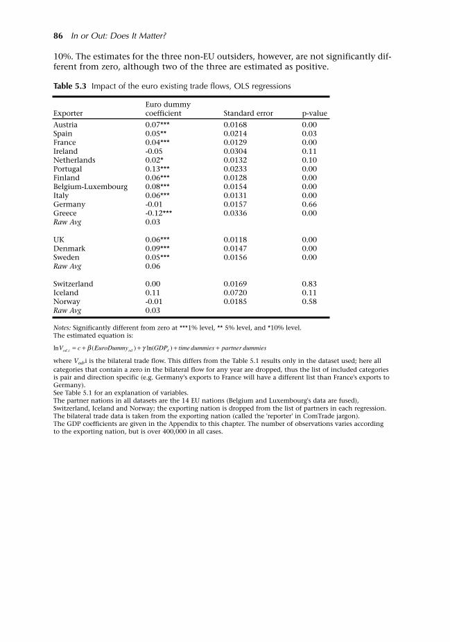
10%. The estimates for the three non-EU outsiders, however, are not significantly dif-ferent from zero, although two of the three are estimated as positive.
86 In or Out: Does It Matter?
Table 5.3 Impact of the euro existing trade flows, OLS regressions
Euro dummyExporter coefficient Standard error p-value
Austria 0.07*** 0.0168 0.00Spain 0.05** 0.0214 0.03France 0.04*** 0.0129 0.00Ireland -0.05 0.0304 0.11Netherlands 0.02* 0.0132 0.10Portugal 0.13*** 0.0233 0.00Finland 0.06*** 0.0128 0.00Belgium-Luxembourg 0.08*** 0.0154 0.00Italy 0.06*** 0.0131 0.00Germany -0.01 0.0157 0.66Greece -0.12*** 0.0336 0.00Raw Avg 0.03
UK 0.06*** 0.0118 0.00Denmark 0.09*** 0.0147 0.00Sweden 0.05*** 0.0156 0.00Raw Avg 0.06
Switzerland 0.00 0.0169 0.83Iceland 0.11 0.0720 0.11Norway -0.01 0.0185 0.58Raw Avg 0.03
Notes: Significantly different from zero at ***1% level, ** 5% level, and *10% level.The estimated equation is:
where Vod,i is the bilateral trade flow. This differs from the Table 5.1 results only in the dataset used; here allcategories that contain a zero in the bilateral flow for any year are dropped, thus the list of included categoriesis pair and direction specific (e.g. Germany's exports to France will have a different list than France's exports toGermany).See Table 5.1 for an explanation of variables.The partner nations in all datasets are the 14 EU nations (Belgium and Luxembourg's data are fused),Switzerland, Iceland and Norway; the exporting nation is dropped from the list of partners in each regression.The bilateral trade data is taken from the exporting nation (called the 'reporter' in ComTrade jargon). The GDP coefficients are given in the Appendix to this chapter. The number of observations varies accordingto the exporting nation, but is over 400,000 in all cases.
dummiespartnerdummiestimeGDPEuroDummycV dodiod ++++= )ln()(ln , γβ
The costs and benefits of joining the euro area involve a simple trade off according tothe traditional view (called the optimal currency area theory, or OCA to cognoscenti):
The costs come at the macro level. By embracing the ECB's one-size-fits-allpolicy, the joiner can no longer tailor its monetary policy to nationalstabilization needs.
The benefits are at the micro level. By eliminating the national currency, thenation integrates more tightly with the euro area economy and this boostseconomic efficiency. A standard gauge of this gain is the trade-enhancing impactof the common currency. A standard story is that the boosted trade is caused bya common-currency-induced reduction in transaction costs among euro areanations.
This report marshals empirical evidence on the size of the micro gains as proxied bythe size of the pro-trade effect. Six main findings are extracted from existing empiricalresearch.
(1) The pro-trade effect of the euro (i.e. the Rose effect) is modest somewherebetween 5% and 15%.
(2) It happened very quickly, appearing already in 1999.
(3) It was not exclusive; euro-usage boosted imports from non-euro area nationsalmost as much as it boosted imports from euro area partners, i.e. there was notrade diversion.
(4) It involved little or no convergence in euro area prices despite the jump in tradeflows.
These four findings suggest that the primary driver of the pro-trade effect could nothave been a common-currency-induced reduction in transaction costs. If it had been,the extra trade would have been promoted by a quick drop in intra-euro area importprices as the elimination of transaction costs would have acted like a discriminatorytrade liberalization among euro area members. These price drops should have: (a)produced trade diversion (since only the euro area 'ins' share the euro); and (b)produced price convergence as the gap between intra-euro area trade prices narrowed.Since there is no evidence for either (a) or (b), it must have been something else. Thenew evidence presented in this report suggests that the pro-trade effect was caused bythe introduction of new goods. This would explain the lack of price convergence(new goods imply higher trade volumes even with constant prices). The report alsoargues that the mechanism driving trade in new-goods may have been a reduction inthe fixed cost of introducing new goods into euro area markets. This mechanism,which is tantamount to a unilateral product-market liberalization, would account for
87
6 Summary and Policy Implications

the lack of trade diversion (it would raise the profitability of introducing new goodsfrom euro area-based and non-euro area-based exporters).
(5) The pro-trade effect varies a great deal across nations; Spain seems to have beenthe biggest gainer while Greece's gain is estimated to be nil or even negative.
(6) The pro-trade effect varies greatly across sectors, with the gains concentrated inincreasing-returns-to-scale sectors such as machinery & transport equipment,and chemicals. Beverages & tobacco was the biggest gainer, but this may be dueto spurious factors (VAT fraud).
The policy implications of these findings are grouped into two broad categories lessons for potential joiners and lessons for the euro area's 12 members and itseconomic management. To share credit where credit is due, I should note that someof the implications I highlight below are stressed by Lane (2006) in his discussion ofmy draft Chapter 2 (eventually published as Baldwin (2006), but circulated in mid-2005).
6.1 Implications for nations thinking of joining the euro area
Europe's currency union boosted exports of the EU 'outs' to euro area members as wellas intra-euro area exports. The best-estimate figures for these 'internal trade creation'and 'external trade creation' effects are 9% for intra-euro area exports and 7% for non-euro area exports to euro area members. Although there is some disagreement amongauthors on the exact numbers, all researchers find that both numbers are quite lowand the gap between them is a few percentage points at most. The implications forpotential joiners are straightforward, but perhaps somewhat unexpected.
Because the euro area already exists and encompasses three-quarters of the EU25'sGDP, the export prize will be very small for nations who join the euro area. Theexport gain is limited to the difference between the internal-trade-creation number(9%) and the external-trade-creation' number (7%) and this only with respect to otherusers of the euro. The joining nation's imports, by contrast, will rise by 9% from itsfellow euro area members and 7% from the remaining 'outs'. The straightforwardimplication of these two facts is that the joiner's imports should rise substantiallymore than its exports. Indeed, regardless of the overall magnitude of the effects, thelack of trade diversion and the pre-existence of the euro area imply that joinersshould experience a larger rise in their imports than in their exports.
Of course, a permanent shift toward current account deficit is not sustainable. Theusual general-equilibrium corrective mechanisms would come into play. But focusingnarrowly on the trade impact of euro membership, the first round impact would be agreater rise in imports than exports. This result is counter-intuitive if one viewsreduced transaction costs as the main driver, but this view is not supported by datafrom the euro area experience. The evidence presented in the report suggests thateuro adoption acted as a unilateral product market liberalization. (For completeness,I note that some researchers found that euro-usage boosted both imports and exportsof euro area nations. I believe these findings are flawed, but even if they are true thetrade effects for joiners is limited to the difference between the internal and externaltrade effects and so are systematically smaller than estimates of the 'Rose effect' wouldsuggest at first glance.)
88 In or Out: Does It Matter?
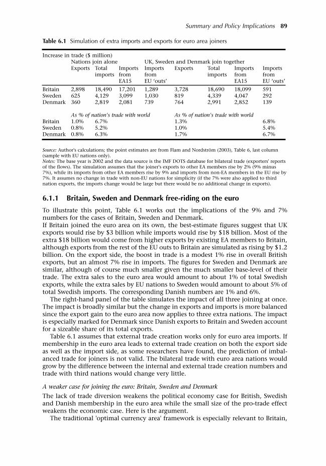
6.1.1 Britain, Sweden and Denmark free-riding on the euro
To illustrate this point, Table 6.1 works out the implications of the 9% and 7%numbers for the cases of Britain, Sweden and Denmark. If Britain joined the euro area on its own, the best-estimate figures suggest that UKexports would rise by $3 billion while imports would rise by $18 billion. Most of theextra $18 billion would come from higher exports by existing EA members to Britain,although exports from the rest of the EU outs to Britain are simulated as rising by $1.2billion. On the export side, the boost in trade is a modest 1% rise in overall Britishexports, but an almost 7% rise in imports. The figures for Sweden and Denmark aresimilar, although of course much smaller given the much smaller base-level of theirtrade. The extra sales to the euro area would amount to about 1% of total Swedishexports, while the extra sales by EU nations to Sweden would amount to about 5% oftotal Swedish imports. The corresponding Danish numbers are 1% and 6%.
The right-hand panel of the table simulates the impact of all three joining at once.The impact is broadly similar but the change in exports and imports is more balancedsince the export gain to the euro area now applies to three extra nations. The impactis especially marked for Denmark since Danish exports to Britain and Sweden accountfor a sizeable share of its total exports.
Table 6.1 assumes that external trade creation works only for euro area imports. Ifmembership in the euro area leads to external trade creation on both the export sideas well as the import side, as some researchers have found, the prediction of imbal-anced trade for joiners is not valid. The bilateral trade with euro area nations wouldgrow by the difference between the internal and external trade creation numbers andtrade with third nations would change very little.
A weaker case for joining the euro: Britain, Sweden and Denmark
The lack of trade diversion weakens the political economy case for British, Swedishand Danish membership in the euro area while the small size of the pro-trade effectweakens the economic case. Here is the argument.
The traditional 'optimal currency area' framework is especially relevant to Britain,
Summary and Policy Implications 89
Table 6.1 Simulation of extra imports and exports for euro area joiners
Increase in trade ($ million)Nations join alone UK, Sweden and Denmark join togetherExports Total Imports Imports Exports Total Imports Imports
imports from from imports from fromEA15 EU outs EA15 EU outs
Britain 2,898 18,490 17,201 1,289 3,728 18,690 18,099 591Sweden 625 4,129 3,099 1,030 819 4,339 4,047 292Denmark 360 2,819 2,081 739 764 2,991 2,852 139
As % of nation's trade with world As % of nation's trade with worldBritain 1.0% 6.7% 1.3% 6.8%Sweden 0.8% 5.2% 1.0% 5.4%Denmark 0.8% 6.3% 1.7% 6.7%
Source: Author's calculations; the point estimates are from Flam and Nordström (2003), Table 6, last column(sample with EU nations only). Notes: The base year is 2002 and the data source is the IMF DOTS database for bilateral trade (exporters' reportsof the flows). The simulation assumes that the joiner's exports to other EA members rise by 2% (9% minus7%), while its imports from other EA members rise by 9% and imports from non-EA members in the EU rise by7%. It assumes no change in trade with non-EU nations for simplicity (if the 7% were also applied to thirdnation exports, the imports change would be large but there would be no additional change in exports).
Sweden and Denmark. All three have economic management institutions that arecapable of running effective independent monetary policies. All three haveeconomies that are large enough and different enough to warrant nationally-tailoredmonetary policies, at least on occasion. In short, giving up their national currencieswould entail a macro cost. This macro cost should be balanced by a micro gain (leav-ing aside high-politics considerations like greater influence in the EU). A mainstay ofsuch gains stems from trade creation.
The UK Treasury's 2003 study on Britain's readiness to join, for example, suggeststhat the microeconomic gains from using the euro may be large. HM Treasury (2003)states that: 'a full union of the 15 current EU Member States including the UK couldraise trade between members by over 40 per cent'. The report then goes on to suggestthat such an increase in trade would boost UK growth and so finds that euro mem-bership would provide large economic gains to Britain. If the real pro-trade effect isjust 10%, as suggested by my report, the Treasury's estimates of the economics gainsmust be scaled back a good deal. Moreover, a good measure of the trade gains theextra exports to euro area nations have already occurred, so the gains to Britain fromactually adopting the euro are correspondingly reduced. To put it differently, the lackof trade diversion means that the economic case for forming a currency bloc amongthe major Continental economies is not the same as the case for joining the bloc onceit exists.
More specifically, Table 6.1 tells us that the boost in trade from joining the euroarea would be modest; this suggests that the case for euro membership is less clearthan previously thought. There are two distinct aspects here. Empirical evidencebased on the euro's actual effects demonstrates that the trade impact of the euro ismore subtle and acts much more like a unilateral trade liberalization than a prefer-ential one. In short, exporters based in the EU 'outs' have had a 'free ride' on the euroarea's formation. Moreover, the overall effect, even for the nations that did join is esti-mated to be small. (HM Treasury (2003), which is otherwise a world-class piece of pol-icy research, uses the 40% trade creation figure that is based on estimates from thepre-euro currency unions; Chapter 2 of this report argues that these estimates areseverely flawed and should be ignored for policy purposes.)
Politics versus economics These numbers suggest a sharp division between the political economy gains and theeconomic gains from euro membership, but explaining this assertion requires somebackground. Standard economic analysis tells us that the major gains from tradecome from importing. The reason is that importing a good allows the nation toconsume at a lower cost. Exports, on the other hand, are basically the price a nationhas to pay to enjoy the privilege of importing. Moreover, if markets are fairlycompetitive, the price a nation receives for its exports reflects the true economic costof the resources used in making them, so exporting per se is a wash from the welfareperspective. Oversimplifying to make the point, the economic welfare perspectiveviews imports as good and exports as bad.
From a political economy perspective, things are just the other way round. Policymakers often hear from exporters who want improved access to foreign markets andthey hear often from domestic firms who want protection from foreign competition.By contrast, consumers who benefit from cheaper imports rarely connect trade poli-cy to the prices they pay in the shops. In this political climate, policies that promoteexports are win-win, politically speaking. Policies that promote imports are a hardsell. Or, to put it crudely, exports are good and imports are bad from the politicaleconomy perspective.
Looking at things from this angle, the 'news' in Table 6.1 is that the political econ-
90 In or Out: Does It Matter?

omy of exports case for membership is much weaker than was suggested in earlierstudies. The lack of trade diversion does less, however, to weaken the economic case.euro membership should boost welfare by boosting imports by 5% or 6%. This is anon-negligible figure even if it is only a one-time step up in efficiency.
Continuing on the political economic of trade axis, it should be noted that the bigexport winners from UK, Swedish and Danish membership would be the euro areanations.
6.1.2 The must-join small members
The traditional view of the costs and benefits of a common currency has littleapplicability to many of the new members of the EU. These nations are so small thatthe macroeconomic cost of embracing the euro is not a cost at all. As Buiter andSiebert (2006) put it crisply: 'Their size and openness imply that for the CE8 [the eightCentral European newcomers], a national currency is a liability.' This is a commonreal-world conclusion one that has led many small nations to abandon theircurrencies in the past. In Europe, for example, Luxembourg abandoned its nationalcurrency in lieu of the Belgian franc, and Monaco to embrace the French franc.Liechtenstein still uses the Swiss franc. As Andres Sutt, deputy governor of the Bankof Estonia said in a July 2005 interview with the Financial Times newspaper: 'youcan't cook a different soup in one corner of the pot'.
Table 6.2 makes the point with figures. The GDPs of the six nations most eager to join(listed in the table) are smaller than that of Luxembourg. Indeed, Malta is so smallthat it makes Luxembourg look like a big economy. For comparison, the table showsFrench cities whose economies are of comparable size. Just as issuing extra currencyin Dijon would do little to stimulate the local economy, pursuing an independentmonetary policy in Estonia would do little good and could open the door to a foreignexchange crisis.
Trade effects for the must-join nations
To these nations, the microeconomic gain is tangential to the membership question,but it may be useful to simulate the trade effects of euro area membership.
The results, shown in Table 6.3, yield broadly the same insights as Table 6.1. euroarea membership will foster tighter economic integration in the sense of makingthese nations especially good importers. Their total imports are projected to riseabout 10%. They will gain on the export side, but since their exporters have alreadybeen benefiting from the single currency in the incumbent euro area nations, thechange will only be modest, in the order of a 1% rise in overall exports.
Summary and Policy Implications 91
Table 6.2 Economic size of the 'must join' nations
GDP at current market prices, French city with equivalent million euros GDP
Malta 4,483 DijonEstonia 10,540 NiceLatvia 12,789 LyonCyprus 13,418 LyonLithuania 20,587 MarseilleSlovenia 27,373 Marseille + NiceLuxembourg 28,637 Marseille + Nice
Source: Eurostat online database for 2005 and author's calculations. The French city equivalent uses the nationalaverage French GDP per capita and city populations to calculate city GDP.
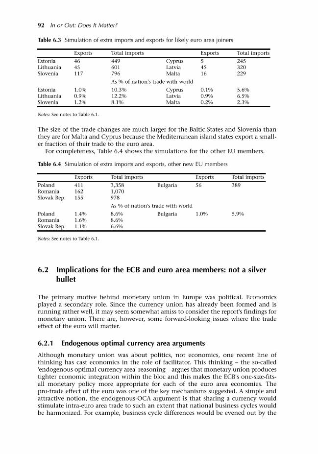
The size of the trade changes are much larger for the Baltic States and Slovenia thanthey are for Malta and Cyprus because the Mediterranean island states export a small-er fraction of their trade to the euro area.
For completeness, Table 6.4 shows the simulations for the other EU members.
6.2 Implications for the ECB and euro area members: not a silverbullet
The primary motive behind monetary union in Europe was political. Economicsplayed a secondary role. Since the currency union has already been formed and isrunning rather well, it may seem somewhat amiss to consider the report's findings formonetary union. There are, however, some forward-looking issues where the tradeeffect of the euro will matter.
6.2.1 Endogenous optimal currency area arguments
Although monetary union was about politics, not economics, one recent line ofthinking has cast economics in the role of facilitator. This thinking the so-called'endogenous optimal currency area' reasoning argues that monetary union producestighter economic integration within the bloc and this makes the ECB's one-size-fits-all monetary policy more appropriate for each of the euro area economies. Thepro-trade effect of the euro was one of the key mechanisms suggested. A simple andattractive notion, the endogenous-OCA argument is that sharing a currency wouldstimulate intra-euro area trade to such an extent that national business cycles wouldbe harmonized. For example, business cycle differences would be evened out by the
92 In or Out: Does It Matter?
Table 6.3 Simulation of extra imports and exports for likely euro area joiners
Exports Total imports Exports Total imports
Estonia 46 449 Cyprus 5 245Lithuania 45 601 Latvia 45 320Slovenia 117 796 Malta 16 229
As % of nation's trade with world
Estonia 1.0% 10.3% Cyprus 0.1% 5.6%Lithuania 0.9% 12.2% Latvia 0.9% 6.5%Slovenia 1.2% 8.1% Malta 0.2% 2.3%
Notes: See notes to Table 6.1.
Table 6.4 Simulation of extra imports and exports, other new EU members
Exports Total imports Exports Total imports
Poland 411 3,358 Bulgaria 56 389Romania 162 1,070Slovak Rep. 155 978
As % of nation's trade with world
Poland 1.4% 8.6% Bulgaria 1.0% 5.9%Romania 1.6% 8.6%Slovak Rep. 1.1% 6.6%
Notes: See notes to Table 6.1.
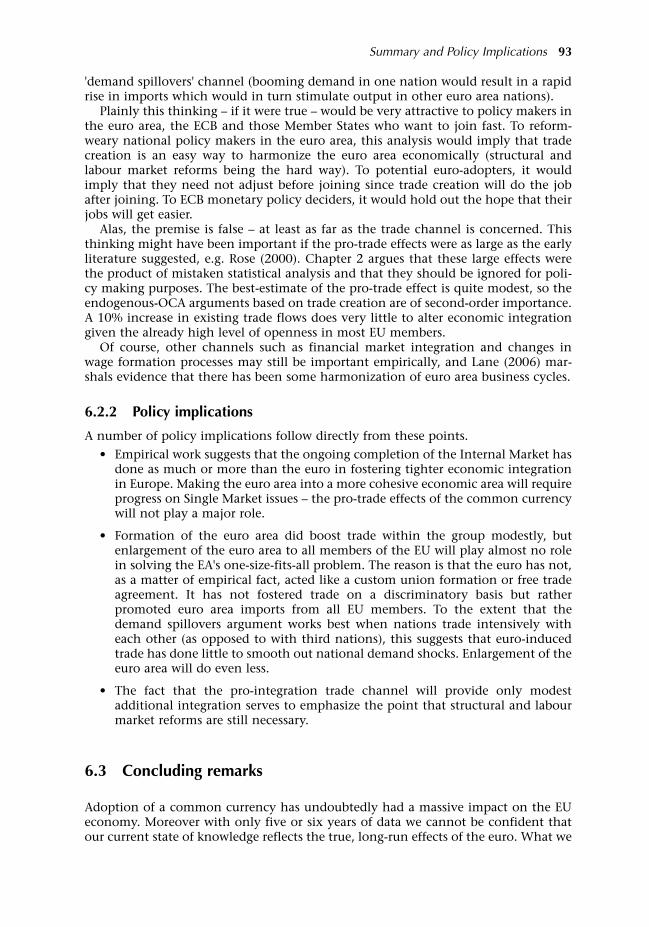
'demand spillovers' channel (booming demand in one nation would result in a rapidrise in imports which would in turn stimulate output in other euro area nations).
Plainly this thinking if it were true would be very attractive to policy makers inthe euro area, the ECB and those Member States who want to join fast. To reform-weary national policy makers in the euro area, this analysis would imply that tradecreation is an easy way to harmonize the euro area economically (structural andlabour market reforms being the hard way). To potential euro-adopters, it wouldimply that they need not adjust before joining since trade creation will do the jobafter joining. To ECB monetary policy deciders, it would hold out the hope that theirjobs will get easier.
Alas, the premise is false at least as far as the trade channel is concerned. Thisthinking might have been important if the pro-trade effects were as large as the earlyliterature suggested, e.g. Rose (2000). Chapter 2 argues that these large effects werethe product of mistaken statistical analysis and that they should be ignored for poli-cy making purposes. The best-estimate of the pro-trade effect is quite modest, so theendogenous-OCA arguments based on trade creation are of second-order importance.A 10% increase in existing trade flows does very little to alter economic integrationgiven the already high level of openness in most EU members.
Of course, other channels such as financial market integration and changes inwage formation processes may still be important empirically, and Lane (2006) mar-shals evidence that there has been some harmonization of euro area business cycles.
6.2.2 Policy implications
A number of policy implications follow directly from these points.
Empirical work suggests that the ongoing completion of the Internal Market hasdone as much or more than the euro in fostering tighter economic integrationin Europe. Making the euro area into a more cohesive economic area will requireprogress on Single Market issues the pro-trade effects of the common currencywill not play a major role.
Formation of the euro area did boost trade within the group modestly, butenlargement of the euro area to all members of the EU will play almost no rolein solving the EA's one-size-fits-all problem. The reason is that the euro has not,as a matter of empirical fact, acted like a custom union formation or free tradeagreement. It has not fostered trade on a discriminatory basis but ratherpromoted euro area imports from all EU members. To the extent that thedemand spillovers argument works best when nations trade intensively witheach other (as opposed to with third nations), this suggests that euro-inducedtrade has done little to smooth out national demand shocks. Enlargement of theeuro area will do even less.
The fact that the pro-integration trade channel will provide only modestadditional integration serves to emphasize the point that structural and labourmarket reforms are still necessary.
6.3 Concluding remarks
Adoption of a common currency has undoubtedly had a massive impact on the EUeconomy. Moreover with only five or six years of data we cannot be confident thatour current state of knowledge reflects the true, long-run effects of the euro. What we
Summary and Policy Implications 93

know as of now, however, alters the fundamental trade-off facing nations that arethinking of joining the euro. Traditionally, a boost in exports is viewed as a political-economy prize to be awarded only to nations that join the euro area. The evidencemarshalled in this report suggests that this is not true. The euro has boosted exportsto the euro area by euro area members and non-members alike. Moreover, the overallsize of the pro-trade effect is modest, in the order of 10%, rather than the much moremassive numbers suggested in previous studies and used in, e.g. HM Treasury (2003).
94 In or Out: Does It Matter?

Appendix A: Summary of the most relevant pricing studies
Appendix A: Summary of the most relevant pricing studies 95
Authors Estimation D e p e n d e n tvariable
Data sources Abstract
Allington,Kattuman,Waldmann(2005)
DIDestimationwith productfixed effectsandnonlinearityin priceconvergence.Treatmentgroup:EMU.Controlgroup: non-EMU.
Coefficient ofvariationacross prices.
Eurostat.Comparativeprice levelindices forindividualconsumptionexpenditurein 200productgroups for allEU countries(1995-2002).
The introduction of the euro was intended tointegrate markets within Europe further, after theimplementation of the 1992 Single MarketProject. Authors examine the extent to which thisobjective has been achieved, by examining thedegree of price dispersion between countries inthe euro area, compared to a control group of EUcountries outside the euro area. We also establishthe role of exchange rate risk in hamperingarbitrage by estimating the euro effect forsubgroups within the euro area, utilizingdifferences among eU countries in participation inthe Exchange Rate Mechanism. Our results, incontrast with previous empirical research, suggestrobustly that the euro has had a significantintegrating effect.
Baye etal.(2002)
Linearregressionwith Euozoneand datedummyvariables.Controls forproduct andmarketstructureeffects.
Log ofaverage pricedifferencebetween EMUand non-EMU.
Kelkoo: Prices(normalizedto France10/2002prices) of acommoditybasket of 28productsFrance, Italy,Netherlands,Spain,Sweden, UK,Denmark.Dates:10/2001;12/2001;01/2002;05/2002.
Authors study the impact of the Euro on pricescharged by online retailers within the EU. Ourdata spans the period before and after the eurowas introduced, covers a variety of products, andincludes countries inside and outside of the euroarea. Our main finding is that the eurochangeover in 2002 neither mitigated pricedifferences nor resulted in purchasing powerparity for products sold online. In fact, evidencesuggests that online prices in the euro areaactually increased compared to prices of EUcountries outside the euro area. Further, contraryto the predictions of purchasing-power-parity, wefind significant differences in the prices chargedby firms both within and across seven countriesin the European Union. We also find significantdifferences in both the average price charged andthe best price available in these countries. Theseconclusions are robust to a variety of controls.
Beck andWeber(2003)
Linearestimate ofprice volatilityas function ofthe distancebetween thelocations andotherexplanatoryvariables. Twosub-periodsused to studythe effects ofthe EMU onthe size of theestimatedbordercoefficients.
Volatility ofthe prices ofsimilar goodssold indifferentlocations.
CPI monthlydata from 81locations.Germany(East andWest), Austria,Finland, Italy,Spain,Portugal andSwitzerland.(January 1991to December2002).
Authors use consumer price data for 81 Europeancities (in Germany, Austria, Finland, Italy, Spain,Portugal and Switzerland) to study the impact ofthe introduction of the euro on goods marketintegration. Employing both aggregated anddisaggregated consumer price index (CPI) data weconfirm previous results which showed that thedistance between European cities explains asignificant amount of the variation in the pricesof similar goods in different locations. We alsofind that the variation of relative prices is muchhigher for two cities located in different countriesthan for two equidistant cities in the samecountry. Under the EMU, the elimination ofnominal exchange rate volatility has largelyreduced these border effects, but distance andborder still matter for intra-European relativeprice volatility.
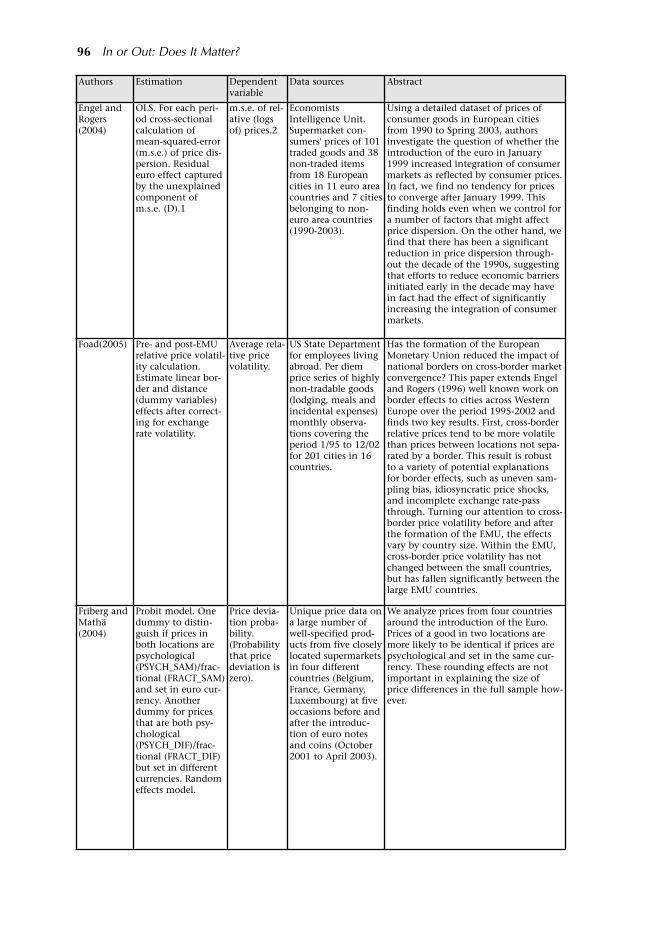
96 In or Out: Does It Matter?
Authors Estimation Dependentvariable
Data sources Abstract
Engel andRogers(2004)
OLS. For each peri-od cross-sectionalcalculation ofmean-squared-error(m.s.e.) of price dis-persion. Residualeuro effect capturedby the unexplainedcomponent ofm.s.e. (D).1
m.s.e. of rel-ative (logsof) prices.2
EconomistsIntelligence Unit.Supermarket con-sumers' prices of 101traded goods and 38non-traded itemsfrom 18 Europeancities in 11 euro areacountries and 7 citiesbelonging to non-euro area countries(1990-2003).
Using a detailed dataset of prices ofconsumer goods in European citiesfrom 1990 to Spring 2003, authorsinvestigate the question of whether theintroduction of the euro in January1999 increased integration of consumermarkets as reflected by consumer prices.In fact, we find no tendency for pricesto converge after January 1999. Thisfinding holds even when we control fora number of factors that might affectprice dispersion. On the other hand, wefind that there has been a significantreduction in price dispersion through-out the decade of the 1990s, suggestingthat efforts to reduce economic barriersinitiated early in the decade may havein fact had the effect of significantlyincreasing the integration of consumermarkets.
Foad(2005) Pre- and post-EMUrelative price volatil-ity calculation.Estimate linear bor-der and distance(dummy variables)effects after correct-ing for exchangerate volatility.
Average rela-tive pricevolatility.
US State Departmentfor employees livingabroad. Per diemprice series of highlynon-tradable goods(lodging, meals andincidental expenses)monthly observa-tions covering theperiod 1/95 to 12/02for 201 cities in 16countries.
Has the formation of the EuropeanMonetary Union reduced the impact ofnational borders on cross-border marketconvergence? This paper extends Engeland Rogers (1996) well known work onborder effects to cities across WesternEurope over the period 1995-2002 andfinds two key results. First, cross-borderrelative prices tend to be more volatilethan prices between locations not sepa-rated by a border. This result is robustto a variety of potential explanationsfor border effects, such as uneven sam-pling bias, idiosyncratic price shocks,and incomplete exchange rate-passthrough. Turning our attention to cross-border price volatility before and afterthe formation of the EMU, the effectsvary by country size. Within the EMU,cross-border price volatility has notchanged between the small countries,but has fallen significantly between thelarge EMU countries.
Friberg andMathä(2004)
Probit model. Onedummy to distin-guish if prices inboth locations arepsychological(PSYCH_SAM)/frac-tional (FRACT_SAM)and set in euro cur-rency. Anotherdummy for pricesthat are both psy-chological(PSYCH_DIF)/frac-tional (FRACT_DIF)but set in differentcurrencies. Randomeffects model.
Price devia-tion proba-bility.(Probabilitythat pricedeviation iszero).
Unique price data ona large number ofwell-specified prod-ucts from five closelylocated supermarketsin four differentcountries (Belgium,France, Germany,Luxembourg) at fiveoccasions before andafter the introduc-tion of euro notesand coins (October2001 to April 2003).
We analyze prices from four countriesaround the introduction of the Euro.Prices of a good in two locations aremore likely to be identical if prices arepsychological and set in the same cur-rency. These rounding effects are notimportant in explaining the size ofprice differences in the full sample how-ever.

Appendix A: Summary of the most relevant pricing studies 97
Authors Estimation Dependentvariable
Data sources Abstract
GoldbergandVerboven(2004)
Estimation of pricedifferentials func-tion on the speedof convergence andlagged price differ-entials.Product/country fixed effectsintroduced. Twosub-periods: 1970-1989 and 1990-2000 to investigatethe effect of inte-gration on pricedispersion.
The depend-ent variableis the firstdifference inthe log-priceof product iin country k(base coun-try Belgium).
Three dimensionalpanel containinginformation onapproximately 150vehicle makes peryear in five distinctEuropean marketsover the period 1970-2000 for Belgium,France, Germany,Italy and the UnitedKingdom.
This paper exploits the unique case ofEuropean market integration to investi-gate the relationship between integra-tion and price convergence in interna-tional markets. Using a panel dataset ofcar prices we examine how the processof integration has affected cross-coun-try price dispersion in Europe. We findsurprisingly strong evidence of conver-gence towards both the absolute andthe relative versions of the Law of OnePrice. Our analysis illuminates themain sources of segmentation in inter-national markets and suggests the typeof institutional changes that can suc-cessfully reduce it.
Imbs et al.(2004)
Fixed effects esti-mation. Dispersionof prices acrossEuropean countries(differences in theTV sets' main char-acteristics areaccounted), as afunction of dis-tance, volatility,language. EMUdummy included.
1. Log ofabsoluteaverage pricedifferencesfor the sameTV set acrosscountrypairs. 2.Bilateralvolatility ofrelativeprices.
GfK France, a privatecompany selling mar-ket surveys based onhigh quality andmuch disaggregateddata. Data on Austria,Belgium, France,Germany, Greece,Italy, theNetherlands,Portugal, Spain,Sweden UK, Hungary,the Czech Republicand Poland andSwitzerland. Timeperiod: 1999-2002.
We use a unique dataset on televisionprices across European countries andregions to investigate the sources ofdifferences in price levels. Our findingsare as follows. (i) Quality is a crucialdeterminant of price differences. (ii)However, sizable international pricedifferentials subsist even for the sametelevision. (iii) EMU countries displaylower price dispersion than non-EMUcountries. (iv) Price dispersion tends tobe smaller regionally than internation-ally. Regional price dispersion is com-parable to intra-EMU dispersion. (v)Absolute price differentials and relativeprice volatility are positively correlatedwith exchange rate volatility. (vi) Brandpremia and relative rankings of brandsdiffer markedly across borders. (vii)Structural estimates allow a more pre-cise quantification of preference het-erogeneity across borders.
Isgut (2002) OLS model of pricedispersion acrosscity pairs determi-nants. Control vari-ables and EMUdummy included.
The disper-sion ofgoods andservicespricesbetween cityi and city j
EconomistIntelligence Unit'sCityData database.Annual observationsof domestic currencyprices for over 160goods and services forup to 123 cities dur-ing the period 1990-2001.
Using two balanced panels of up to124 goods and services prices and up to116 international cities, this paperstudies the determinants of price dis-persion across city pairs in 2001. Usingcontrols for cities located in the samecountry, regional trading areas, com-mon languages and historical links,price dispersion increases with geo-graphical distance, nominal bilateralexchange rate volatility, and differ-ences in economic development. Pricedispersion is significantly lower acrosscities located in the euro area. It is alsolower for cities that use the US dollaror have currencies hard pegged to it,though the effect is less robust.

98 In or Out: Does It Matter?
Authors Estimation Dependentvariable
Data sources Variables
Lutz(2003)
DIDapproach.Treatmentgroup: EMU.Controlgroup: non-EMU.Control vari-ables: the standarddeviation ofexchange rategrowth, the standarddeviation of outputgrowth rates andstandard deviation ofinflation rates.
Estimatedstandarddeviationof the logof commoncurrencyprices.
Four datasets onfinal goods prices forEU member states.Time interval: 1995-2001.1. Prices of BigMacs that are pub-lished annually inThe Economist.2.The cover prices ofThe Economist. 3.Pre-tax car pricesfrom Car Prices inthe European Union,a survey of car pricesregularly released bythe EuropeanCommission.4. Dataon the costs of vari-ous goods and servic-es from Prices andEarnings around theGlobe, a publicationby the Swiss bankUBS.
This paper examines whether Europeanmonetary union has lowered the degree ofprice dispersion among member countries.A number of different estimation methodsare applied to four independent datasetscontaining prices of identical goods.While the results reported in the papervary somewhat across goods, they providelittle overall support of the EuropeanCommission's claim that the single cur-rency would significantly deepen marketintegration among the Eurozone coun-tries. Even though this should be viewedas preliminary evidence, it does suggestthat there are other, more importantimpediments to market integration in theEU.
Mathä(2003)
1. Random effectsestimation of pricesdeviations on dis-tance. Border andmonetary associationdummy included.2.OLS between andproduct specific fixedeffects.
Absolutepercentageprice differ-ence oneproductbetweentwo differ-ent loca-tions.
Price data on 6 dif-ferent supermarkets,on 92 products col-lected at four differ-ent points in time:mid-October 2001,mid- December2001, mid-February2002, and mid-April2002.
This paper uses individual supermarketprices and analyzes to what extentabsolute deviations from the law of oneprice are attributable to transaction costs.The results indicate that absolute percent-age price differences are increasing in dis-tance, but at a decreasing rate. Similarly,crossing borders increases price deviations,while being inside the former Belgian-Luxembourg monetary association has theopposite effect. This result nurtures thehopes that the euro may be able to reduceregional and cross-border price differencesin the long term. Furthermore, larger dif-ferences in packaging sizes result in largerprice deviations, while the opposite is thecase for prices observed within the sameretail group.
Parsleyand Wei(2001)
Linear regression ofprices dispersion ona set of independentvariables as distance,instrumental (i.e. tar-iff rates) and institu-tional (i.e. tradeblocks) variables.City and time fixedeffects. Euro dummyincluded.
Standarddeviationof prices.
EconomistIntelligence Unit.Panel dataset of 95goods and 83 cities(one city per coun-try) during 1990-2000.
This paper studies the effects of instru-mental and institutional stabilizationexchange rate volatility on the integrationof goods markets. Rather than using dataon volume of trade, this paper employstri-dimensional panel of prices of 95 verydisaggregated goods in 83 cities aroundthe world during 1990-2000. Authors findthat the impact of an institutional stabi-lization promotes market integration farbeyond an instrumental stabilization.Among them, long-term currency unionsare more effective than more recent cur-rency boards. All have room to improverelative to a US benchmark.
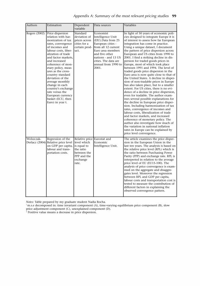
Notes: Table prepared by my graduate student Nadia Rocha.1 m.s.e decomposed in: time invariant component (A), time-varying equilibrium price component (B), slowprice adjustment component (C), unexplained component (D).2 Positive value means a decrease in price dispersion.
Appendix A: Summary of the most relevant pricing studies 99
Authors Estimation Dependentvariable
Data sources Variables
Rogers (2002) Price dispersionrelation with har-monization of taxrates, convergenceof incomes andlabour costs, liber-alization of tradeand factor markets,and increasedcoherence of mon-etary policy, meas-ures as the cross-country standarddeviation of theaverage monthlychange in eachcountry's exchangerate versus theEuropean currencybasket (ECU, thenEuro) in year t.
Standarddeviation ofprices acrosscities for acertain prod-uct.
EconomistIntelligence Unit(EIU).Data from 25European cities -from all 12 currentEuro area membersand five othernations - and 13 UScities. The data areannual from 1990 to2001.
In light of 50 years of economic poli-cies designed to integrate Europe it isof interest to assess how far Europeanintegration has come in practice.Using a unique dataset, I documentthe pattern of price dispersion acrossEuropean and US cities from 1990 to2001. I find a striking decline in dis-persion for traded goods prices inEurope, most of which took placebetween 1991 and 1994. The level oftraded goods price dispersion in theEuro area is now quite close to that ofthe United States. A decline in disper-sion of non-tradable prices in Europehas also taken place, but to a smallerextent. For US cities, there is no evi-dence of a decline in price dispersion,even for tradable. The author exam-ines several possible explanations forthe decline in European price disper-sion. Including harmonization of taxrates, convergence of incomes andlabour costs, liberalization of tradeand factor markets, and increasedcoherence of monetary policy. Theauthor also investigate how much ofthe variation in national inflationrates in Europe can be explained byprice level convergence.
Wolszczak-Derlacz (2004)
Regression of theRelative price levelon GDP per capita,labour and trans-portation costs.
Relative pricelevel whichis equal tothe ratiobetween thePPP and theexchangerate.
Eurostat andEconomicIntelligence Unit.
The article examines the price disper-sion in the European Union in thelast ten years. The analysis is based onthe relative price level (RPL) which isthe ratio between Purchasing PowerParity (PPP) and exchange rate. RPL isinterpreted in relation to the averageprice level of EU (EU15-100). Theanalysis of price convergence is exam-ined on the aggregate and disaggre-gates level. Moreover the regressionbetween RPL and GDP per capita,labour costs and transportation cost istested to measure the contribution ofdifferent factors in explaining theobserved convergence pattern.
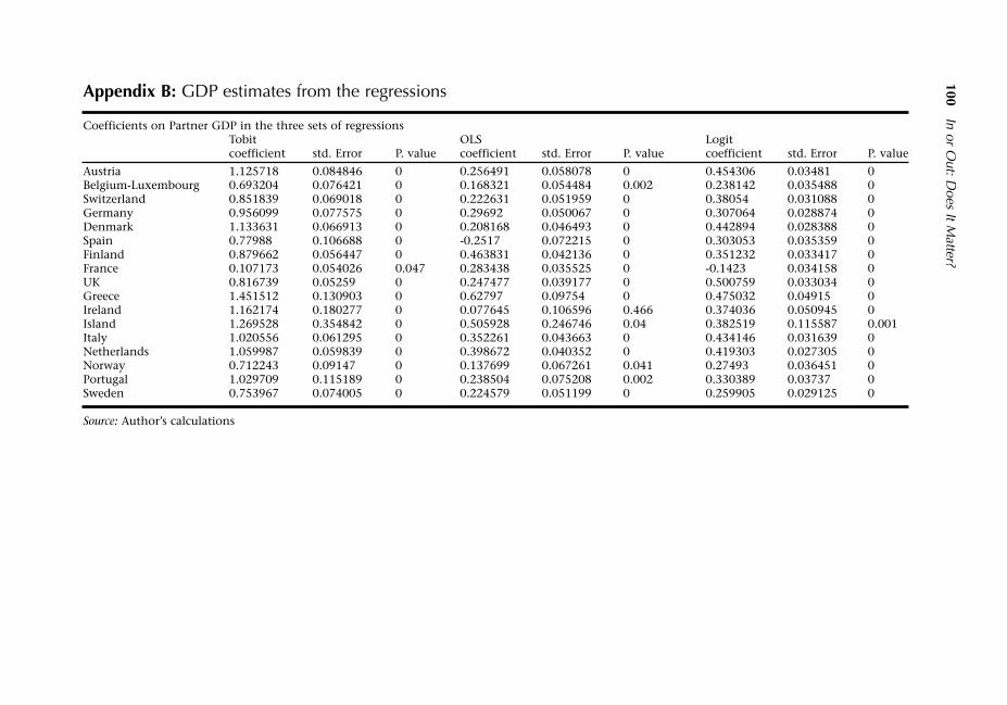
100In or O
ut: Does It M
atter?
Appendix B: GDP estimates from the regressions
Coefficients on Partner GDP in the three sets of regressionsTobit OLS Logitcoefficient std. Error P. value coefficient std. Error P. value coefficient std. Error P. value
Austria 1.125718 0.084846 0 0.256491 0.058078 0 0.454306 0.03481 0Belgium-Luxembourg 0.693204 0.076421 0 0.168321 0.054484 0.002 0.238142 0.035488 0Switzerland 0.851839 0.069018 0 0.222631 0.051959 0 0.38054 0.031088 0Germany 0.956099 0.077575 0 0.29692 0.050067 0 0.307064 0.028874 0Denmark 1.133631 0.066913 0 0.208168 0.046493 0 0.442894 0.028388 0Spain 0.77988 0.106688 0 -0.2517 0.072215 0 0.303053 0.035359 0Finland 0.879662 0.056447 0 0.463831 0.042136 0 0.351232 0.033417 0France 0.107173 0.054026 0.047 0.283438 0.035525 0 -0.1423 0.034158 0UK 0.816739 0.05259 0 0.247477 0.039177 0 0.500759 0.033034 0Greece 1.451512 0.130903 0 0.62797 0.09754 0 0.475032 0.04915 0Ireland 1.162174 0.180277 0 0.077645 0.106596 0.466 0.374036 0.050945 0Island 1.269528 0.354842 0 0.505928 0.246746 0.04 0.382519 0.115587 0.001Italy 1.020556 0.061295 0 0.352261 0.043663 0 0.434146 0.031639 0Netherlands 1.059987 0.059839 0 0.398672 0.040352 0 0.419303 0.027305 0Norway 0.712243 0.09147 0 0.137699 0.067261 0.041 0.27493 0.036451 0Portugal 1.029709 0.115189 0 0.238504 0.075208 0.002 0.330389 0.03737 0Sweden 0.753967 0.074005 0 0.224579 0.051199 0 0.259905 0.029125 0
Source: Authors calculations
1 See http://www.econlib.org/library/Enc/GoldStandard.html.
2 Published in 1991 as 'On the Microeconomics of the European Monetary Union'.
3 Bini Smaghi (1991).
4 Jeffery Frankel has posted photos of the event athttp://ksghome.harvard.edu/~jfrankel/ECB%20June2005pixJF&RB.htm. His uneditedcomment is at http://ksghome.harvard.edu/~jfrankel/BaldwinECB-RoseEffectdAug05.pdf.
5 Standard references for the gravity model are Tinbergen (1962), Pöyhönen(1963a), Linnemann (1966), Anderson (1979), Bergstrand (1985) and Helpmanand Krugman (1985). It was reintroduced to US academic circles by McCallum(1995) and Frankel and Wei. (1993).
6 I believe the Rose trade data has a systematic bias in it, what I call the silver-medal mistake below.
7 This section is based on Baldwin and Taglioni (2006); see that paper for a moreformal treatment of the theory and econometrics.
8 See Baldwin and Taglioni (2006), or the original presentation by Anderson andvan Wincoop (2001).
9 See Jeffery Frankel's discussion in Baldwin (2006) for an account of why no onebefore Rose asked the currency union question empirically.
10 Note that when Glick and Rose (2002) run their regression without the timedummies, their estimated coefficient on the CU dummy is one standarddeviation larger than it is with time dummies, so it can be important to correctthe small problem.
11 In his chapter on the gravity model, Feenstra (2003) shows an equation with thelog of the sums, rather than the sum of the logs. The theory leading up to this,however, is developed in the context of the simplest trade model - i.e. theKrugman trade model without trade costs. In this model, all bilateral flows areidentical so the sum of the logs does equal the log of the sums. However, whentrade costs are introduced, the theory does not necessarily predict bilaterallybalanced trade; real-world trade flows are often very unbalanced, especiallybetween big and small nations.
12 If x = yδ, ln[(x + y)/2] = lnx + ln(1+δ) - ln2, while ln(xyδ)/2 = ln(x) + ln(δ)/2. Thewrong way minus the right way is ln(1+δ) - lnδ/2 - ln2; this difference gets largeas δ deviates from unity.
13 Formally, if one asks the statistics whether the country dummies should beexcluded from Rose-Wincoop, the answer is no. They belong. Therefore, the Roseeffect estimates performed without them are null and void.
101
Endnotes

14 Bill Bryson, in his book Mother Tongue, claims that this aphorism is ancient, sothat we should read 'proves' using its archaic meaning, 'tests', as in provinggrounds.
15 Glick and Rose (2001) show a figure for Anglo-Irish that looks quite different;they use the level of trade which drops due the second oil-shock recession. Thomand Walsh look at the bilateral trade as a share of all Irish exports and thuscontrol somewhat for the global recession.
16 Note that Rose (2000) does roughly this with his difference-in-differenceregression that is reported in the text but not in a table; the Rose effect this yieldsis only 17% more trade.
17 By the way, these suspicions of mine were raised by the similarity of the twodifferent techniques applied on two separate datasets. It would be interesting tomake a more direct comparison, to see what the Rose-Wincoop country-dummytechnique would yield on the Glick-Rose dataset, and what the Glick-Rose pairdummy technique would yield on the Rose-Wincoop dataset. Such comparisonswould help us to judge the importance of the omitted variable critique, and thevalidity of the Glick-Rose solution of throwing in one pair dummy for the wholeperiod.
18 Actually you can see it, since Economic Policy posts the Panel drafts on its website:www.economic-policy.org.
19 By the way, this nonlinearity is consistent with Krugman's famous Home MarketEffect whereby a nation's exports are affected by its size.
20 It would be interesting to see the share of trade pairs with common currencies byyear, but this is not reported in Glick-Rose; only the full panel average isreported.
21 See Baldwin and Robert-Nicoud (2002) for an explanation based on sunk costs.
22 Tenreyro has a recent paper on the impact of exchange volatility on trade thatapplies the same IV strategy. Her conclusion is that volatility has no effect ontrade, which is strange given her early findings on the CU dummy. Strangely, thispaper, Tenreyro (2001), excludes the common currency variable altogether andindeed never mentions it. Maybe it would have been too jarring to have acommon currency boosting trade many times over, but lower volatility havingno impact. Or, maybe she, like Rose, decided that IV estimation of the Rose effectwas a dead end.
23 Actually, since France includes some small, poor, open and remote islands(Outré-Mers), we could test whether the euro boosted trade between these islandsand the nations that were not in the DM bloc-franc fort complex, say, Greece,Portugal, Spain, Finland and Ireland.
24 This literature review draws on Gomes et al. (2004).
25 Here is Andy's email to me (I was a Managing Editor of Economic Policy at thetime): 'Respected Editors, Ernesto Stein (and co-authors) at the IADB has juststarted to circulate a short paper which analyzes the effect of EMU on intra-EMUtrade using data from the first couple of years of EMU. He shows the effect issignificant (about 15-25% after just two years), using only data from the EU15and also a larger sample of developed countries. I'm obviously biased (though Ishould say that I'm trying to escape this particular sub-literature). But it's ofobvious policy relevance for Europe and the ancestors of his work appear inEconomic Policy, so I think it's of potential interest to you. Anyway, now that I'vealerted you to it, I've done my duty to God and the Queen.'
102 In or Out: Does It Matter?
26 Full disclosure: I was the Managing Editor who did the rewriting. I probablyshould have already mentioned that Andy Rose and I were PhD classmates atMIT 1982-86.
27 MSO, like many authors in this literature, use EMU to stand for 'Europeanmonetary union'; unfortunately, EMU stands for 'Economic and MonetaryUnion' - at least since the Maastricht Treaty that implemented EMU in bothcorrect and incorrect senses. All EU members are part of EMU, so writers who arefamiliar with European integration use the terms euro area, Euroland or euro areato refer to those EU members who have adopted the euro. Also EA is shorter thanEMU.
28 Just to take one example, the EU signed dozens of preferential trade agreementsduring the 1992-2002 period. Since each of these erodes the preference marginof EU members, they should alter intra-EU trade flows.
29 In fact, MSO should probably have used 1993-2002 data since the new datacollection systems started with 1993 data.
30 The pair dummies are time-invariant and thus miss part of the Anderson-vanWincoop point of using time-varying country dummies, but given the shortperiod, one can hope that the omission is not too important. Moreover, someoneshould redo MSO's estimates with time-varying country dummies (obviously inthis case one cannot also include pair dummies).
31 Note that MSO try to control for the observable part of this, but the measure theyuse is extremely crude and so surely fails to fully control for this. Seehttp://europa.eu.int/comm/internal_market/score/index_en.htm.
32 More formally, MSO statistically reject the pooling hypothesis that would benecessary for the estimates without dummies to make sense.
33 They write: 'If dollar prices of goods produced in the euro area fall as a result ofdepreciation, the value of trade between two EMU countries will fall as well,relative to trade between other countries, and the EMU effect on trade couldpotentially be underestimated. One way to deal with this issue would be tocontrol for bilateral unit value indices in order to capture the change in importand export prices. Unfortunately, these indices are not available. For this reason,in order to control for these valuation effects we include in most regressions anindex of the real exchange rate for each of the countries in the pair (the index isthe ratio between the nominal exchange rate of each country vis-à-vis the USdollar and the country's GDP deflator). Reassuringly, the inclusion of theseindices does not change the results significantly.'
34 Their pair dummies correct for the relative-prices-matter term on average butAnderson-VanWinccop showed us that this term should vary over time;moreover, the relative-prices-matter term definitely includes bilateral exchangerates between the USA and each importing nation so a spurious correlation isassured.
35 Forcing the pair dummy to be the same for a half century is a bit strained,although all authors using the Glick-Rose data do this. For example, surely theFranco-German dummy was strongly negative in the first part of the sample andstrongly positive in the last part. It would be interesting to see what happens ifthey allow, for example, decadal pair dummies.
36 This idea was to figure out how much of Britain's superior macro performancewas due to their decision to stay out of the euro area, but with so few data pointsthis proved elusive.
Endnotes 103
37 The numbers for Greece, Portugal and Finland are not significantly different tozero, except Greece's EA1 estimate which is significant at the 5% level ofconfidence.
38 To be more precise, the demand equation is Xod = no(pod/Pd)−σ(Ed/Pd) where Xod is thevolume of o's exports to d.
39 In particular the impact will be multiplied by nation-i's expenditure share innation-d's market.
40 ComTrade doesn't report non-traded goods (zeros); it was possible to square thedatabase by inserting categories for which a nation has exported at least once toat least one destination, but not included are those categories which neverexported to anyone during the period considered.
41 Dividing this total we see that there are about 2,500 zeros in the average outsiderexport vector to the average EA nation. This means about half the possible goodsare not exported, although of course the number varies by market (there are farfewer zeros in Switzerland's export vector to Germany than its export vector toPortugal, for example).
42 That is, the time dummies and the constant will be perfectly collinear with anynation-o variable.
43 Norway and Iceland are in the European Economic Area and Switzerland hasbilateral agreements with the EU, but these do not grant full Single Market status.For example, the lack of a customs union with the EU means that this trade issubject to distortionary rules of origin.
104 In or Out: Does It Matter?

105
Alesina, A., Barro, R.J. and Tenreyro, S. (2002), 'Optimal Currency Areas', HarvardInstitute Research Working Paper No. 1958, June.
Alho, K. (2002), 'The Impact of Regionalism on Trade in Europe', Royal EconomicSociety Annual Conference 2003, 3, Royal Economic Society.
Allington, N., Kattuman, P. and Waldmann, F. (2005), 'One Market, One Money, OnePrice?', International Journal of Central Banking, 2005, pp. 73-115.
Anderson, J. E. (1979), 'A Theoretical Foundation for the Gravity Equation', AmericanEconomic Review, 69(1), pp. 106-16.
Anderson, J. and van Wincoop, E. (2001), 'Gravity with Gravitas: A Solution to theBorder Puzzle', NBER Working Paper No. 8079, January.
Anderton, R., Baltagi, B., Skudelny, F. and De Souza, N. (2002) 'Intra- and Extra-EuroArea Import Demand for Manufactures', European Trade Study Group AnnualConference, 2002, 4, European Trade Study Group.
Anderton, R., Baldwin, R. and Taglioni, D. (2003), 'The Impact of Monetary Union onTrade Prices', ECB Working Paper No. 238, June.
Andrews, D.W.K. (2003), 'End-of-Sample Instability Tests', Econometrica, 71(6), pp.1661-94.
Artis, M.J. (2002), 'Reflections on the Optimal Currency Area (OCA) criteria in thelight of EMU', Oesterreichische Nationalbank Working Paper No. 69, July.
Artis, M. and Zhang, W. (1995), 'International Business Cycles and the ERM: Is Therea European Business Cycle?', CEPR Discussion Paper No. 1191.
Asplund, M. (2002), 'Risk Averse Firm in Oligopoly', International Journal of IndustrialOrganization.
Augier, P., Gasiorek, M. and lai Tong, C. (2005), 'The Impact of Rules of Origin onTrade Flows', Economic Policy, 20(43), pp. 567-624.
Baldwin, R. (1991), 'On the Microeconomics of the European Monetary Union',European Economy, Special Issue No. 1, 'One Market, One Money', EuropeanCommission, Brussels.
Baldwin R. (2005), 'Heterogeneous Firms: Testable and Untestable Properties of theMelitz Model', NBER Working Paper No. 11471, May.
Baldwin, R. (2006), The euros trade effect, ECB Working Paper 594, March.
Baldwin, R. and Di Nino, V. (2006), 'Testing for the Euro's Impact on the ExtensiveMargin of Trade: What Do We Learn From Zeros?', HEI manuscript, March.
Baldwin, R. and Robert Nicoud, F. (2002), Entry and Assymetric Lobbying: WhyGovernments Pick Losers, NBER Working Paper No.8756.
References

Baldwin, R. and Taglioni, D. (2005), 'Positive OCA Criteria: Microfoundations for theRose Effect', March (http://hei.unige.ch/~baldwin/TradeEffectsEuroBaldwin.html).
Baldwin R. and Taglioni, D. (2006), 'Gravity for dummies and Dummies for Gravity(Equations)', manuscript.
Baldwin, R., Bertola, G. and Seabright, P. (2003), EMU: Assessing the Impact of the Euro,Blackwell Publishing Ltd, Oxford.
Baldwin, R., Skuderlny, F. and Taglioni, D. (2005), 'Trade Effects of the Euro: Evidencefrom Sectoral Data', European Central Bank, Working Paper No. 446.
Barr, D., Breedon, F. and Miles, D. (2003), 'Life on the Outside', Economic Policy, 18,pp. 573-613.
Baye, M., Gatti, R., Kattuman, P. and Morgan, J. (2002), 'Online Pricing and the EuroChangeover: Cross Country Comparisons', Judge Institute of ManagementWorking Paper 17 (forthcoming in Economic Inquiry).
Beck, G. and Weber, A. (2003), 'How Wide are European Borders? On the IntegrationEffects of Monetary Unions', Center of Financial Studies Economic Paper No.2001/07, Revisited.
Berger, H. and Nitsch, V. (2005), 'Zooming Out: The Trade Effect of the Euro inPerspective', CESifo Working Paper No. 1435.
Bergin, A., Fitz Gerald, J. and McCoy, D. (2004), 'How Has Economic ManagementEvolved Within EMU', Paper presented at the Annual Kenmare EconomicWorkshop, October, http://www.esri.ie/pdf/Economic_Wkshop_Oct04.pdf.
Bergstrand, J. (1985), 'The Gravity Equation in International Trade: SomeMicroeconomic Foundations and Empirical Evidence', Review of Economics andStatistics, 67(3), pp. 474-81.
Bernard, A.B., Eaton, J., Jenson, J.B. and Kortum, S. (2000), 'Plants and Productivity inInternational Trade', NBER Working Paper No. 7688.
Bernard, A. and Jensen, B. (2004), 'Exporting and Productivity in the USA', OxfordReview of Economic Policy, 20(3).
Bini-Smaghi, L. (1991), 'Exchange Rate Variability and International Trade: Why is itso Difficult to Find any Empirical Relationship?', Applied Economics, 23, pp. 927-36.
Buiter, W. and Sibert, A. (2006), Eurozone Entry of New EU Member States from Central Europe: Should They? Could They?,http://www.nber.org/~wbuiter/eurozone.pdf.
Bun Maurice, J.B. and Klaassen, F. (2002), 'Has the Euro increased Trade?', TinbergenInstitute Discussion Papers, TI 2002 108-2, October.
Bun Maurice, J.B. and Klaassen, F. (2004), 'The Euro Effect on Trade is not as Large asCommonly Thought', Tinbergen Institute Discussion Papers No. 2003-086/2,October.
De Nardis, S. and Vicarelli, C. (2003a), 'The Impact of Euro on Trade: The (Early) Effectis not so Large', European Network of Economic Policy Research Institutes,Working Paper No. 017.
De Nardis, S. and Vicarelli, C. (2003b), 'Currency Unions and Trade: The Special Caseof EMU', World Review of Economics, 139(4), 625-49.
De Souza, L.V. (2002), 'Trade Effects of Monetary Integration in Large, MatureEconomies', A Primer on European Monetary Union, Kiel Working Paper No. 1137.
De Souza, J. and Lamotte, O. (2006), 'Does Political Disintegration Lead to TradeDisintegration? Evidence from Former Yugoslavia', Manuscript.
106 In or Out: Does It Matter?
Deardorff, A. (1998), 'Determinants of Bilateral Trade: Does Gravity Work in aNeoclassical World?', in Jeffrey Frankel (ed.), The Regionalization of the WorldEconomy, University of Chicago Press.
Dell'Arricia, G. (1998), 'Exchange Rate Fluctuations and Trade Flows: Evidence fromthe European Union', IMF Working Paper No. WP98/107.
Devereux, Michael B. and Lane, Philip R. (2003), Understanding Bilateral ExchangeRate Volatility, Journal of International Economics 60, pp. 109-132.
Engel, C. and Rogers, J.H. (2004), 'European Product Market Integration after theEuro', European Policy 19(39), pp. 347.
European Commission (1990) One Market, One Money, European Economy 44.
European Commission (2000), 'Report from the Commission to the Council and theEuropean Parliament', COM(2000), 28 final.
European Commission (2004), 'The Internal Market Index 2004', DG Joint Research,July, available at http://webfarm.jrc.cec.eu.int/uasa/doc/Tarantola/IMI_2004/The%20Internal%20Market%20Index%202004.pdf.
Evenett, S.J. and Wolfang, K. (2002), 'On Theories Explaining the Success of theGravity Equation', Journal of Political Economy 110, pp. 281-316 .
Feenstra, R. (2003), Advanced International Trade, Princeton University Press,Princeton, NJ.
Fidrmuc, J. and Fidrmuc, J. (2003), 'Disintegration and Trade', Review of InternationalEconomics, 11, p. 811.
Flam H. and Nordström, H. (2003) 'Trade Volume Effects of the Euro: Aggregate andSector Estimates', Institute for International Economic Studies, unpublished.
Foad, H. (2005), 'Europe without Borders? The Effect of the EMU on Relative Prices',available at http://ssrn.com/abstact=514502.
Frankel, J.A. (1997), Regional Trading Blocs in the World Economic System, Institute forInternal Economics, Washington, DC.
Frankel J. (2003), 'The UK Decision RE EMU. Implications of Currency Blocs for Tradeand Business Cycle Correlations', in Submissions on EMU from Leading Academics,HM Treasury, London, pp. 99-109.
Frankel, J.A. and Rose, A.K. (1996), 'The Endogeneity of the Optimum Currency AreaCriteria', NBER Working Paper No. 5700.
Frankel, J.A. and Rose, A.K. (1998), 'The Endogeneity of the Optimum Currency AreaCriteria', Economic Journal, 108, July, pp. 1009-25.
Frankel, J.A. and Rose, A.K. (2000), 'Estimating the Effect of Currency Unions onTrade and Output', NBER Working Paper No. 7857, August.
Frankel, J. and Wei, S-j. (1993), 'Trade Blocs and Currency Blocs', NEBR Working PaperNo. W4335.
Friberg, R. and Mathä, T.Y. (2004), 'Does a Common Currency Lead to (More) PriceEqualisation? The Role of Psychological Pricing Points', Economic Letters, 84, pp.281-7.
Gagnon, J.E. (2003), 'Long-Run Supply Effects and the Elasticities Approach', FRBInternational Finance Discussion Paper No. 754.
Glick, R. and Rose, A. (2001), 'Does a Currency Union Affect Trade? The Time SeriesEvidence', European Economic Review, 46(6), pp. 1125-51.
Goldberg, P.K. and Knetter, M.M. (1997), 'Goods Prices and Exchange Rates: WhatHave We Learned?', Journal of Economic Literature, 35(3), pp. 1243-72.
References 107
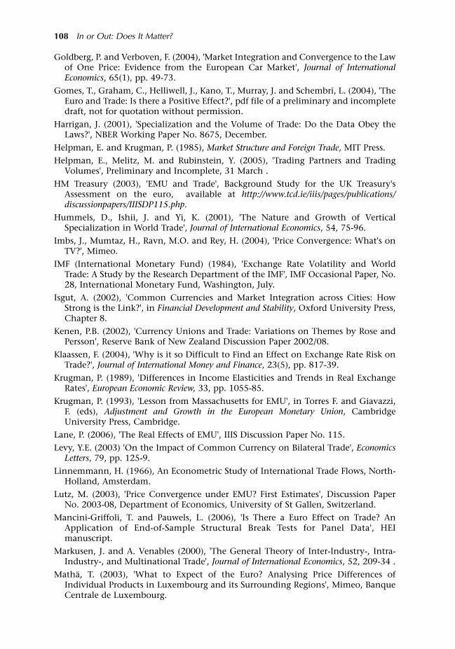
Goldberg, P. and Verboven, F. (2004), 'Market Integration and Convergence to the Lawof One Price: Evidence from the European Car Market', Journal of InternationalEconomics, 65(1), pp. 49-73.
Gomes, T., Graham, C., Helliwell, J., Kano, T., Murray, J. and Schembri, L. (2004), 'TheEuro and Trade: Is there a Positive Effect?', pdf file of a preliminary and incompletedraft, not for quotation without permission.
Harrigan, J. (2001), 'Specialization and the Volume of Trade: Do the Data Obey theLaws?', NBER Working Paper No. 8675, December.
Helpman, E. and Krugman, P. (1985), Market Structure and Foreign Trade, MIT Press.
Helpman, E., Melitz, M. and Rubinstein, Y. (2005), 'Trading Partners and TradingVolumes', Preliminary and Incomplete, 31 March .
HM Treasury (2003), 'EMU and Trade', Background Study for the UK Treasury'sAssessment on the euro, available at http://www.tcd.ie/iiis/pages/publications/discussionpapers/IIISDP115.php.
Hummels, D., Ishii, J. and Yi, K. (2001), 'The Nature and Growth of VerticalSpecialization in World Trade', Journal of International Economics, 54, 75-96.
Imbs, J., Mumtaz, H., Ravn, M.O. and Rey, H. (2004), 'Price Convergence: What's onTV?', Mimeo.
IMF (International Monetary Fund) (1984), 'Exchange Rate Volatility and WorldTrade: A Study by the Research Department of the IMF', IMF Occasional Paper, No.28, International Monetary Fund, Washington, July.
Isgut, A. (2002), 'Common Currencies and Market Integration across Cities: HowStrong is the Link?', in Financial Development and Stability, Oxford University Press,Chapter 8.
Kenen, P.B. (2002), 'Currency Unions and Trade: Variations on Themes by Rose andPersson', Reserve Bank of New Zealand Discussion Paper 2002/08.
Klaassen, F. (2004), 'Why is it so Difficult to Find an Effect on Exchange Rate Risk onTrade?', Journal of International Money and Finance, 23(5), pp. 817-39.
Krugman, P. (1989), 'Differences in Income Elasticities and Trends in Real ExchangeRates', European Economic Review, 33, pp. 1055-85.
Krugman, P. (1993), 'Lesson from Massachusetts for EMU', in Torres F. and Giavazzi,F. (eds), Adjustment and Growth in the European Monetary Union, CambridgeUniversity Press, Cambridge.
Lane, P. (2006), 'The Real Effects of EMU', IIIS Discussion Paper No. 115.
Levy, Y.E. (2003) 'On the Impact of Common Currency on Bilateral Trade', EconomicsLetters, 79, pp. 125-9.
Linnemmann, H. (1966), An Econometric Study of International Trade Flows, North-Holland, Amsterdam.
Lutz, M. (2003), 'Price Convergence under EMU? First Estimates', Discussion PaperNo. 2003-08, Department of Economics, University of St Gallen, Switzerland.
Mancini-Griffoli, T. and Pauwels, L. (2006), 'Is There a Euro Effect on Trade? AnApplication of End-of-Sample Structural Break Tests for Panel Data', HEImanuscript.
Markusen, J. and A. Venables (2000), 'The General Theory of Inter-Industry-, Intra-Industry-, and Multinational Trade', Journal of International Economics, 52, 209-34 .
Mathä, T. (2003), 'What to Expect of the Euro? Analysing Price Differences ofIndividual Products in Luxembourg and its Surrounding Regions', Mimeo, BanqueCentrale de Luxembourg.
108 In or Out: Does It Matter?

McCallum, J. (1995), 'National Borders Matter: Canada-US Regional Trade Patterns',The American Economic Review, 85(3), pp. 615-23.
Melitz J. (2001), 'Geography, Trade and Currency Union', CEPR Discussion Paper No.2987, October.
Melitz, M. (2003), 'The Impact of Trade on Intraindustry Reallocations and AggregateIndustry Productivity', Econometrica, 71, pp. 1695-725.
Melitz, M.J. and Ottaviano, G.I.P. (2003), 'Market Size, Trade and Productivity', June,6.
Micco, A., Stein, E. and Ordoñez, G. (2003a), 'The EMU Effect on Trade: What's in itfor the UK?', Inter-American Development Bank, July.
Micco, A., Stein, E. and Ordoñez, G. (2003b), 'The Currency Union Effect on Trade:Early Evidences from EMU', Economic Policy, 37, October, pp. 317-56.
Mongelli, P., Dorrucci, E. and Agur, I. (2005), 'What Does European InstitutionalIntegration Tell Us About Trade Integration?', ECB Occasional Paper, 40.
Mundell, R.A. (1961), 'A Theory of Optimum Currency Areas', The American EconomicReview, 51(4), pp. 657-65.
Neary, J.P. and Leahy, D. (2000), 'Strategic Trade and Industrial Policy towardsDynamic Oligopolies', Economic Journal, 110(463), pp. 484-508.
Nitsch, V. (2002), 'Honey I Shrunk the Currency Union Effect on Trade', WorldEconomy, 25(4), pp. 457-74.
Obstfeld, M. and Rogoff, K. (2000), 'The Six Major Puzzles in InternationalMacroeconomics: Is there a Common Cause?', NBER Macroeconomics Annual2000, MIT Press.
Pakko, M.R. and Wall, H.J. (2001), 'Reconsidering the Trade-Creating Effects of aCurrency Union', Federal Reserve Board of St Louis Review, 83(5), 37-45.
Parsley, D.C. and Shang-jin, W. (2001), 'Limiting Currency Volatility to StimulateGoods Market Integration', NBER Working Paper No. 8468.
Persson, T. (2001), 'Currency Unions and Trade: How Large is the Treatment Effect?',Economic Policy, 33, October, pp. 435-48.
Piscitelli, L. (2003), Mimeo, UK Treasury.
Pöyhönen, P. (1963a), 'A Tentative Model for the Volume of Trade Between Countries',Welwirtschaftliches Archiv, 90(1), 93-9.
Pöyhönen, P. (1963b), 'Toward a General Theory of International Trade', EkonomiskaSamfundets Tidskrift, 16(2), 69-78.
Rocha, N. (2006), Fixed Trade Cost Liberalization in a Multi-Nation World: RoseEffect without Trade Diversion, GIS manuscript, PhD.
Rogers, J. (2002), 'Monetary Union, Price Level Convergence, and Inflation: HowClose is Europe to the United States?', International Finance Discussion Paper No.740, Board of Governors of the Federal Reserve System, Washington, DC .
Rose, A.K. (1999), 'One Money, One Market: Estimating the Effect of CommonCurrencies on Trade', CEPR Working Paper No.7432, December.
Rose, A.K. (2000a), 'One Money, One Market: Estimating the Effect of CommonCurrencies on Trade', Economic Policy, 30, 7-46.
Rose, A.K. (2000b), 'EMU's Potential Effect on British Trade: A QuantitativeAssessment', 4 July.
Rose, A.K. (2001a), 'Currency Unions and Trade: The Effect is Large', Economic Policy,33, pp. 449-61.
References 109

Rose, A.K. (2001b), 'EMU and Swedish Trade', 9 November.
Rose, A.K. (2002), 'Honey the Currency Union Effect on Trade hasn't blown up', TheWorld Economy, 25(4), April.
Rose, A. and Stanley, D. (2004), 'A Meta-Analysis of the Effect of Common Currencieson International Trade', Journal of Economic Surveys, 19, p. 347.
Rose, A.K. and van Wincoop, E. (2000), 'National Money as a Barrier to InternationalTrade: The Real Case for Currency Union', http://faculty.haas.berkeley.edu/arose/.
Rose, A.K. and van Wincoop, E. (2001), 'National Money as a Barrier to Trade: TheReal Case for Monetary Union', American Economic Review, 91(2), 386-90.
Ruffles, D., Tily J. and Caplan, D. (2003), 'VAT Missing Trader Intra-CommunityFraud: The effect on Balance of Payments Statistics and UK National Accounts',www.statistics.gov.uk/articles/economic_trends/ETAug03Ruffles.pdf.
Silva, S. and Tenreyro, S. (2003), 'Gravity-Defying Trade', Federal Reserve Bank ofBoston Working Paper No. 03-01, 9 January.
Taglioni, D. (2002), Exchange Rate Volatility as a Barrier to Trade: NewMethodologies and Recent Evidence, Open Economies Review 7, pp. 493-499.
Tenreyro, S. (2001), 'On the Causes and Consequences of Currency Unions', HarvardUniversity, Mimeo.
Tenreyro, S. and Barro, R.J. (2003), 'Economic Effects of Currency Unions', NBERWorking Paper 9435.
Thom, R. and Walsh, B. (2002), 'The Effect of a Currency Union on Trade: LessonsFrom the Irish Experience', European Economic Review, 46, pp. 1111-23.
Tinbergen, J. (1962), Shaping the World Economy: Suggestions of an InternationalEconomic Policy, New York: The Twentieth Centiry Fund.
Wei, S-J. (1999), 'Currency Hedging and Goods Trade', European Economic Review, 43,pp. 1371-94.
Wolszczak-Derlacz, J. (2004), 'One Europe, One Product, Two Prices: The PriceDisparity in the EU', Paper presented at the 3rd International Conference of theEEFS, 'World Economy and European Integration' University of Gdansk, Sopot, 13-16 May.
Wyplosz, C. (1997), 'EMU: Why and How it May Happen?', Journal of EconomicPerspectives, 11, Fall, pp. 3-22.
Yi, K. (2003), 'Can Vertical Specialization Explain Growth of World Trade?', Journal ofPolitical Economy, February, pp. 52-102.
110 In or Out: Does It Matter?