Does it matter how happiness is measured? Evidence from a ...
27
Does it matter how happiness is measured? Evidence from a randomized controlled experiment * Raphael Studer Department of Economics, University of Zurich November 2011 Abstract: A continuous and a discrete rating scale were implemented for a single item happiness question in a representative survey. A randomized controlled experiment enables unique analyses on data quality and distributions, which suggest superiority of the continuous scale. Results raise doubts about earlier inferences drawn on correlates of happiness. So far only self-assessed discrete happiness data have been used for research into the determinants of happiness. However, distribution distortions were found for the numerically labeled discrete scale, especially for women. Through this discretization bias, the widely reported gender happiness inequality puzzle can be explained. Keywords: happiness, subjective well-being, life satisfaction, likert scale, visual analogue scale, rating scales, gender inequalities, gender gap JEL Codes: C81, I31 * Address for correspondence: University of Zurich, Department of Economics, Z¨ urichbergstr. 14, CH- 8032 Z¨ urich, Switzerland, T +41 44 634 22 97, k [email protected] I thank Rainer Winkelmann for useful comments and Maarten Streefkerk for assistance in data preparation. Funding from the Candoc Forschungskredit of the University of Zurich is gratefully acknowledged. This paper draws on data of the LISS panel of CentERdata.
Transcript of Does it matter how happiness is measured? Evidence from a ...

Does it matter how happiness is measured?Evidence from a randomized controlled
experiment∗
Raphael Studer
Department of Economics, University of Zurich
November 2011
Abstract: A continuous and a discrete rating scale were implemented for a single item
happiness question in a representative survey. A randomized controlled experiment enables
unique analyses on data quality and distributions, which suggest superiority of the continuous
scale. Results raise doubts about earlier inferences drawn on correlates of happiness. So far
only self-assessed discrete happiness data have been used for research into the determinants of
happiness. However, distribution distortions were found for the numerically labeled discrete
scale, especially for women. Through this discretization bias, the widely reported gender
happiness inequality puzzle can be explained.
Keywords: happiness, subjective well-being, life satisfaction, likert scale, visual analogue
scale, rating scales, gender inequalities, gender gap
JEL Codes: C81, I31
∗ Address for correspondence: University of Zurich, Department of Economics, Zurichbergstr. 14, CH-8032 Zurich, Switzerland, T+41 44 634 22 97, k [email protected] thank Rainer Winkelmann for useful comments and Maarten Streefkerk for assistance in data preparation.Funding from the Candoc Forschungskredit of the University of Zurich is gratefully acknowledged. Thispaper draws on data of the LISS panel of CentERdata.
1 Introduction
Interest in the determinants of subjective well-being using survey data has burgeoned in
recent years. Research is often based on happiness or life satisfaction data self-assessed by
survey participants on a Likert scale (LS) (Likert, 1932). Even though the discrete rating
scale is widely accepted, its properties, e.g. cardinality remain disputed (Kristoffersen,
2010). However, little has been done to find better alternatives. This study proposes a
new continuous rating scale to measure individual happiness, the visual analogue scale
(VAS). Results of the randomized controlled experiment identify stylized happiness facts
as question design artifacts and strongly suggest the use of the VAS.
Many scholars have been interested in the design of the single item happiness question.
It was Fordyce (1987) who proposed to assess happiness on a single item 11-point LS. But
other rating scales have been tested (Diener, 1994). The effect of labels on LS scores was
examined by Larsen et al. (1984). Differences among countries in interpretation of LS
labels was studied using satisfaction vignettes (Kapteyn et al., 2010). Cummins (2003)
investigated LS of variable discriminating power. Andrews and Crandall (1976) assessed
data quality of 7-point LS, faces and ladder scales. However, all these rating scales remained
discrete.
Van Praag and Ferrer-i-Carbonell (2004) noted that individuals likely perceive satisfac-
tion as a continuous phenomenon bounded by the states of complete dissatisfaction and
complete satisfaction. This statement seems to be widely accepted. For instance, ordered
response models are used for LS happiness data and build on a continuous latent frame-
work. But the necessary discretization of the underlying true happiness score into a LS
score may lead to systematic transformation error. This stands in contrast to a continuous
rating scale which may be perceived as a reference continuum of the latent happiness. Such
a rating scale is the VAS.
The VAS (Hayes and Patterson, 1921) is simply a bounded line. Respondents assess
their happiness by setting a marker on the VAS. The VAS has been extensively used in
1

medical pain research (McCormack et al., 1988). With the development of computer based
surveys, the accuracy and simplicity of implementation of the VAS has jumped up. A
recent literature has compared LS and VAS in computer based experiments (Couper et al.,
2006). But to my knowledge there have been only four happiness studies implementing the
VAS (Matsubayashi et al., 1992; Saris et al., 1998; Bouazzaoui and Mullet, 2002; Hofmans
and Theuns, 2008). Saris et al. (1998) did not declare how the “graphical line scale” was
implemented and for which satisfaction domain it was used. The other three articles are
small sample paper and pencil vignette studies, which do not have any counterfactual for
the VAS scores, i.e. LS scores for the same individuals. This study proposes to close this
gap.
The present paper is the first to implement the VAS for a single item happiness ques-
tion in a representative survey. A unique randomized controlled experiment enables the
identification of question design effects. Thanks to a large set of socioeconomic and so-
ciodemographic variables heterogeneous mode effects can be identified and patterns and
puzzles which occurred so far with LS data can be explained. The analyses conclude in
favor of the VAS.
The article starts by presenting the survey and question design and assessing the quality
of the experiment. Section 3 reviews the existing literature on comparison of single item
happiness scales and provides among others estimates for reliability and validity measures.
I conclude on equally reliable and valid data quality for both scales. Distributional analyses
are presented in Section 4. The experiment shows the same people to be on average less
happy when they use the VAS. Moreover, wider spread happiness scores appear for the
VAS. Higher variance can be attributed to an increased likelihood of scoring closer to
the extremes. In fact, the unexplained pattern of LS high frequency categories is due to
too little discriminating power. Section 5 exploits the existence of two parallel happiness
questions to investigate the impact of rating scales on correlates of happiness for a common
set of respondents. All statistically significant determinants of happiness, except gender,
2

are found to correlate stronger in absolute values with the VAS happiness scores than with
the LS scores. The significant gender gap which is present when LS data is used vanishes
with the use of VAS data. This study demonstrates that answer distortions of female
respondents exist in the discrete numerically labeled measurement. This finding is in line
with an earlier study (Conti and Pudney, 2011). Section 6 concludes.
2 Survey Design
The randomized controlled experiment used in this paper was implemented in the Lon-
gitudinal Internet Studies for the Social Sciences (LISS). The LISS panel was established
by CentERdata based at Tilburg University in the Netherlands. 10’150 random addresses
were drawn from a 10% sample of the Dutch population register. The oldest inhabitant
was approached by a letter including 10 Euros. In case of non-response, the person was
called or visited. 5176 households agreed to participate in the survey. Households without
broadband internet connection or computer were provided with it. During the first survey
year in 2007, the average monthly answer rate was 73% of all members of participating
households (Scherpenzeel, 2009). Knoef and de Vos (2009) concluded on underrepresenta-
tion of elderly people and of some ethnicities. In 2009, a refreshment sample stratified by
age, ethnicity and household types was successful in establishing representativeness of the
LISS panel (de Vos, 2010).
A monthly e-mail invites participants to respond to the LISS panel. Monthly waves
consist of three questionnaires. The Background Variable questionnaire needs only be up-
dated if any changes in core socioeconomic or sociodemographic variables, such as income,
education, age, civil status or household composition, occurred. A second questionnaire
contains questions on one of the twelve Core Studies repeated every year, for instance on
health or religion. A third questionnaire contains an Assembled Study, like the experiment
analyzed in this paper. Survey respondents can choose which questionnaire they want to
3

answer first.
The experiment was implemented during the survey months March and April 2011.
The web link to the Assembled Study directed participants to a single item happiness
question. Answers had to be given either on a LS or a VAS. Answer scales were randomly
assigned in March at the moment people opened the questionnaire. In the subsequent
month, the scales were changed or again randomly assigned if people had not answered
during the March wave. In the best case scenario, every survey participant reported his or
her happiness using the VAS and the LS. This crossover design has two advantages. First,
the dependent sample increases power of test statistics. Second, any time effect affecting
only subgroups of the sample is captured in both scales equally and does not distort the
analysis.
The crossover experiment is summarized in figure 1. The samples consist of 5042 par-
ticipants in wave 1 and 4795 participants in wave 2. The paired sample, individuals who
responded in March and April 2011, includes 4274 observations. In May 2011, the month
after the experiment took place, the LISS Core Study was dedicated to the personality
questionnaire. This personality study gathers not only information on overall happiness on
a LS ranging from 0 to 10 (11 points) but also on personality traits, like emotional stability
or self esteem. 5230 individuals responded to the personality questionnaire in May, out of
which 3770 individuals had already assessed their happiness in March and April. Data of
the March and April waves will be uniquely used to quantify differences in means, variances
(section 4) and correlates (section 5). For the assessment of data quality (section 3) data
of the May wave will be employed additionally.
Screenshots of the two questions implemented in the experiment are presented in figure
2. The LS ranges from 0-9 (10 points). The VAS is a continuous line. It neither caries
numbers nor does it show categories. However, for practical purposes, a scale unit has to
be chosen for the VAS. In this application VAS scores were covertly measured from 0 to
99. Therefore, the VAS measurement has ten times more discriminating power than the LS
4
measurement. In order to ensure comparability of the two rating scales, VAS scores were
divided by 11. Hence, in all analyses that follow, VAS and LS scores are comprised inside
the closed interval from 0 to 9. The design of both scales was the same: No questions were
asked before the happiness question; the length of both scales was approximately equivalent;
the VAS had no default marker to avoid artificial high frequency regions (Treiblmaier and
Filzmoser, 2009); both scales were aligned horizontally, however, results should not differ to
vertical scales (Funke et al., 2010; Paul-Dauphin et al., 1999); and the same anchor words
were used for the LS and the VAS in order to avoid wording effects (Weng, 2004). I expect
no hidden factors to drive any differences in responses between the two rating scales.
In order to examine the question design, participants answered 5 evaluation questions
after participating in the experiment. Difficulty in answering, clearness of the question,
degree of thought provocation, interest and joyfulness while responding were rated on a
LS ranging from 1 (certainly not) to 5 (certainly yes). Figure 3 gives the distributions by
scale types to all five evaluation questions. Distributions are very similar. A Kolmogorov
Smirnov test rejects equality of distributions only for the question clearness. However, also
for this question, densities in the five categories do not differ by more than 1 percentage
point. Given this evidence, I conclude on absence of design artifacts causing response
problems.
Two concerns about the experiment may still be raised. First, screen resolution may
differ among survey participants. A lower resolution leads to a wider VAS or LS. Previous
empirical findings however suggest no effect of varying length of the VAS (Keindler et al.,
2003). Second, people can decide on the order of the three questionnaires each month on
their own. Order of questionnaires have been shown to have important effects on answers
(Schumann and Presser, 1981), however as will be shown it does not affect mean answers
in this survey.
Table 1 and 2 examine the quality of the present experiment. First, table 1 evaluates
whether the subsamples are truly random by comparing the means of ex-ante characteristics
5

by scale types. Equality of means for any of the variables, except for out of labor force,
working and foreigner cannot be rejected. However, the point estimates are very similar
in magnitude for the two groups and differ only by 2-3 percentage points for these three
variables. If randomization seems not complete in these three variables statistically, it is
practically. The picture is similar for the April wave. Second, table 2 reports estimates of
the parameters capturing a time or questionnaire order effect, if existent. The following
model is estimated using the paired sample.
sit = β0 + β1 · aprilit + β2 · vasit + β3 · aprilit · vasit (1)
+ β4 · experiment2ndit + β5 · vasit · experiment2ndit + εit
The dependent variable sit is the happiness score. The parameter β1 estimates a poten-
tial time effect, which differs between scales through the interaction term β3. The variable
experiment2ndit takes the value 1 if during the 2 hours preceding the response of the hap-
piness question, the Background Variable questionnaire was opened. This questionnaire
order effect may also vary by scales through the interaction coefficient β5. Table 2 shows
that neither a time nor a questionnaire order effect exist for one or the other scale. It is
concluded that the experiment was successful and that the findings presented below are
only caused by different rating scales.
3 Validity and reliability of the VAS
A simple quality measurement of rating data is provided by the true score model (e.g., Saris
and Gallhofer, 2007). Consider the observed score si for individual i being a noisy measure
of the transformed score ti: sij = tij + ζij. If the transformation for every rating scale j
is a linear function of the latent happiness hi: tij = vj · hi + ηij, then substitution yields:
sij = vj · hi + εij. The three parameters of interest v2j for all three rating scales at hand
6
(j = {vas, ls10, ls11}) are identified through the three correlations between the different
sij’s. In fact corr(si,vas; si,ls10) = vls10·vvas·V ar(hi)√V ar(si,ls10)·V ar(si,vas)
, which reduces to corr(si,vas; si,ls10) =
vls10 · vvas if equality of variances is assumed. The lowest quality is found for the VAS
(0.66) and equal quality for the two discrete measurements (0.71). However, this result is
misleading. The estimates for v2j are equal tov2j
V ar(si,j), if only the variance of the latent
happiness (V ar(hi)) is normalized to one. The next section will show that the variance of
VAS scores is higher than the variances of the two LS scores. Therefore, VAS data quality
in the true score model is smaller than those of the discrete rating scales, because VAS
scores are wider spread. Better measurements for data quality have to be found.
Recent computer surveys experimentally implementing the LS and VAS used various
methods to examine survey data. The item response time has been recorded. While Funke
and Reips (forthcoming) found no difference, Cook et al. (2001) and Couper et al. (2006)
have reporeted a longer response time for the VAS. Completion rates of questionnaires have
been lower and questions were skipped more often if the VAS instead of the LS was used
(Couper et al., 2006). Answers were modified nearly twice as often with the VAS (Funke
and Reips, forthcoming). The data structure does not allow the analysis of all of these
indicators.
In the experiment, randomization only took place when participants accessed the ques-
tionnaire. Therefore, item non-response cannot be assessed. Moreover, all participants
finished the questionnaire and completion rates do not differ. This study finds higher aver-
age item response times for the VAS (16 seconds) than for the LS (10 seconds). However,
this may be due to a difference in question design: the VAS question had one sentence
more to read (figure 2). A higher fraction of survey participants was found to move back
to adjust the happiness score for the VAS (2.3%) than for the LS (1.4%). This may simply
indicate a lack of familiarity with the VAS as opposed to the LS.
Validity and reliability seem the most established measures to assess survey data quality.
Validity quantifies the degree to which the rating scale is able to capture the true latent
7

construct. A systematic error due to a nonconformity of a rating scale harms validity.
Intuitively, the LS, requesting the categorization of a continuous feeling, may have lower
validity than the VAS. Reliability is the extent to which the rating scale can reproduce its
measurements. Low reliability is due to a random measurement error. The high sensitivity
of the VAS may lead to lower reliability. Different methodologies have been established to
investigate validity and reliability of rating scales.
A huge body of literature on reliability and validity of the LS and the VAS can be
found in medical pain research. Validity has been tested by the administration of different
intensities of heat (Price et al., 1994) or sound (Lara-Munoz et al., 2004) in a randomized
order. Survey participants had to rate the level of pain on a LS or VAS. Flint et al. (2000)
assessed reliability by letting people judge hunger feelings during two subsequent days
while the authors controlled ingested energy. These three studies and all studies, which
were reviewed, have either not been advising against the VAS or concluded in favor of it.
Happiness cannot be measured objectively, like heat or sound. The presence of validity
in single item happiness responses has been evaluated through content or convergent validity
(Diener, 1994). Content validity has been assessed by the correlation between individual
happiness scores of different rating scales. Only marginal differences between the three
implemented scales are observed. First, the VAS correlates with the Likert 11 and 10
point scales by 0.69, whereas the two discrete measurements correlate by 0.72 (table 8).
Magnitude of these point estimates is in line with earlier findings (e.g., Larsen et al.,
1984). The positive correlations may indicate that all three measures assess the same
latent construct, but cannot conclude which scale is best. Convergent validity in contrast
ranks scales. In happiness research this has been done with the magnitudes of correlations
between happiness scores and personality traits. This analysis therefore relies implicitly on
the assumption of a valid scale of the external criterions, which are in most cases multiple
item LS questions. Estimates of correlations between rating scales (columns) and the BIG
V inventory (Goldberger, 1992) or the self-esteem scale (Rosenberg, 1965) are reported
8

in table 4. These six trait variables were gathered in the personality study of the May
wave. Personality traits are judged stable (e.g., Srivastava et al., 2003) though the time
gap between the assessment of happiness (March, April, May) and personality traits (May)
causes no problems. The magnitude of correlations are similar to earlier research (e.g.,
Larsen et al., 1984 or Abdel-Khalek, 2006). No pattern in lower or higher convergent
validity for one scale is discovered. The VAS should be considered as a valid happiness
scale, at least if the 10 or 11 point LS are judged as being it.
Reliability of single item happiness questions has been assessed through test-retest re-
liability. The test-retest method uses the same sample and the same measurement on two
occasions. Larsen et al. (1984) and Krueger and Schkade (2008) have concluded on test-
retest reliability coefficients ranging from 0.4 to 0.6 for single item discrete measurements.
The data structure of this study does not allow to present test-retest reliability coefficients.
Reliability can also be exploited using the experiment. It was shown that randomization
was successful and that no time effect exists. Sample distributions in happiness scores
should be equal between the March and April waves for each rating scale if the scales are
reliable. In order to compare distributions among the two scales, the VAS score was split
up in 10 equal intervals. Figure 4 shows the histograms for both waves for both scales.
A huge agreement in the distribution in scores is observed. It could be judged marginally
stronger for the VAS. The VAS is considered to be a reliable rating scale for happiness.
Survey happiness data assessed by a LS are widely accepted to be of good quality, i.e.
to be valid and reliable. The existing methods to assess data quality suggest no exorbitant
differences between the VAS and the LS. Moreover, the theoretical argument should be
emphasized again. At least higher (theoretical) validity should be attributed to the VAS,
because it overcomes idiosyncratic discretization and the line length acts as a reference
continuum to represent perceived happiness.
9

4 The distribution of happiness scores
Several computer based studies have reported equality in distributions between VAS and
LS scores (e.g., Couper et al. 2006 or Funke and Reips, forthcoming). However, these
studies have not asked people to assess subjective feelings, such as happiness. All of them
have used objective judgments, as questions on clothing style or vignettes on behavior. A
paper and pencil study on self reported individual coping reported lower mean values for
the VAS (Flynn et al., 2006). Hence, distributions may be expected to differ.
Table 5 reports the first and second moments of both happiness scales, the LS and
the VAS. t-tests on the equality of means and Levine’s tests on the equality of variances
for each wave and for the paired sample are presented. All three samples show the same
picture: lower mean but wider spread happiness scores in the case of the VAS. All null
hypotheses of equality of means and variances can be rejected.
The random assignment of response scales creates a control group (LS) of individuals
that should have the same outcomes as what the treatment group (VAS) would have had
if they had answered on the LS. The simple comparison in means therefore suggests that
participants would have reporeted 0.45 points higher happiness on the LS than on the
VAS. Due to the experimental set-up, controlling for a large set of socioeconomic and
sociodemographic variables, such as age, household size, employment and marital status,
gender, origin and education, does not change the point estimates but increases precision
only. For a decomposition of the treatment effect in population subgroups readers are
referred to the next section.
The difference in mean happiness may result from the comparison of a discrete mea-
surement and a continuous measurement. For instance, VAS scores would be artificially
lower, if a LS score of 9 maps an interval of latent happiness ranging from 8.5 to 9.4, but a
VAS score of 9 represents a latent happiness of 9 only. In order to eliminate the influence of
differences in perceptions, VAS scores were transformed into discrete scores and the mean
comparison was repeated. To discretize the VAS, the line was divided into ten equally
10

spaced intervals. The intervals were assigned the LS scores 0 to 9 in ascending order from
left to right. The first column of table 6 shows once more the first and second moments
for the LS. Means and variances for discrete VAS scores are presented in the second col-
umn. The difference in means suggests that participants would have been around 0.25
points happier on the LS than on the VAS. The treatment effect is lower compared to the
previous analysis, but stays significant, negative and large. Hence, people are on average
happier on the LS than on the VAS.
The second finding reported in table 5 is an increase in variances of 0.8 points, when
moving from the LS to the VAS. Wider spread happiness scores contain more information.
However, higher variance in the VAS scores may simply be due to the high sensitivity of the
scale. For instance, people would like to cross the equivalent of a 7 but crossed 6.8 instead.
The thesis of inexactness can be easily tested. First, if it holds true, than the discretized
VAS should have lower variance. Table 6 shows the contrary: the variance increases by
another 0.5 points. Second, distributions of happiness scores give more evidence that not
the higher sensitivity is the trigger of higher variances. Figure 6 plots a histogram for
the LS scores and a kernel density estimate for the VAS scores of the March wave. For
the latter the Epanechnikov kernel and the bandwidth that minimizes the mean integrated
squared error (bandwidth = 0.23) are used. Two patterns can be found. First, response
densities are lower in the categories 7 and 8. Second, people are more likely to score close
to the two boundaries. Higher variance is in part explained by a shift in answers towards
the extremes.
The differences in distributions can be quantified. Three variables indicating the loca-
tion of the scores on the discretized scales are generated. All indicator variables are equal
to 0 except that the first is 1 if the individual answered a 7 or 8, the second is 1 if the score
was equal to 1, 2 or 3 and the last is 1 if a 9 was observed. For each of these indicator
variables a linear probability model is estimated using the paired sample. A large set of so-
cioeconomic and demographic variables as well as a wave dummy and dummies indicating
11

the questionnaire and question order are included in the regression. Table 7 reports the
estimates of the parameter of interest, i.e. the average effect of the VAS on the probability
of scoring in one of these intervals. All effects were found to be large and significant. The
probability that a participant scores a 7 or 8 is reduced by over 21 percentage points if the
VAS was used. This effect can be divided in the two effects prevailing at the extremes. In
the case of the VAS the probability of a 9 is more than 8 percentage points higher and the
probability of scoring either a 1, 2 or 3 is more than 2 percentage points higher. The shifts
in distributions are substantial.
The higher variance in VAS scores due to more extreme answers reveals the LS high
frequency categories as a scale artifact. An earlier international comparison concluded
on Dutch people being more likely to avoid extreme LS values (Kapteyn et al., 2007).
But the present results show that even Dutch respondents are willing to score closer to
the boundary, but not at the boundary itself. A continuous measurement with infinitely
fine categories enables respondents to approach the boundaries and thus overcomes answer
distortions caused by a too insensitive answer scale.
5 The correlates of happiness
Research into the determinants of subjective well-being has burgeoned in recent years,
and valuable insights have been obtained (e.g., Kahneman and Krueger, 2006). Scholars
have been interested in the effects of schooling (Orepolus, 2003), income (Easterlin, 1995),
unemployment (Winkelmann and Winkelmann, 1998) or age (Stone et al., 2010). Many
findings have been replicated for different countries and have been judged as robust (Frey
and Stutzer, 2002). All these studies use discrete happiness data. Therefore, the question
arises: How much are these findings affected by the specificities of the LS?
The paired sample consists of the same set of respondents assessing their happiness
either on the VAS or the LS. From March to April, no individual reported changes in
12
core socioeconomic or sociodemographic variables. Regressions for both scales of happiness
scores on a set of socioeconomic and sociodemographic variables should estimate the same
effects. Any changes in correlates when moving from one to the other scale can be attributed
to the scale design.
Table 8 shows estimates by scale types of a linear regression modeling happiness scores
as dependent variable. Results for the LS are in line with the research literature (e.g.
Kahneman and Krueger, 2006 or Frey and Stutzer, 2002). Happiness is found to be U-
shaped in age, foreigners and unemployed are less and women more happy. Marriage and
house ownership, the latter may be interpreted as a proxy for savings, have a positive effect
on happiness. However, these findings do not carry over to the VAS regression.
Comparison of the LS correlation coefficients with those of the VAS sample reveals some
striking findings. Signs of statistically significant explanatory variables stay the same. But
the equality of coefficients is rejected by a Chow test (p-value = 0.012). Except for the
male dummy, effects of statistically significant variables are in absolute values stronger in
the VAS regression. These findings need some investigation.
Happiness data is generally criticized to contain a mix of short and long term circum-
stances. If the explanatory variables in the regression are judged as indicators for long term
factors, higher coefficients of statistically significant variables raise the question whether
the VAS scores contain more information on long term factors causing well-being. Due
to the wider spread VAS scores the VAS regression model has to explain more variance.
However, the R2 remain the same for both regressions (0.09). This indicates that the model
explains more absolute variance, but that in both regressions the same relative amount of
error variance is present. Both scales seem to capture to the same degree short and long
term factors causing happiness.
The most powerful finding reported in table 8 is the change in statistical significance
of the gender variable. In the LS sample men are found to be 0.162 points less happy
than women. This is a huge effect. For instance, a male with an average income must be
13
compensated with an income increase of 17% to make him at least as well off as his female
counterpart. When the VAS sample is used, the happiness gender inequality vanishes.
The disappearance of the gender gap indicates that subgroups of the population may
be influenced to different degrees by rating scale design. In order to identify heterogeneous
effects, the difference in happiness scores is computed for every individual. The LS score is
subtracted from the VAS score and the difference regressed on the same set of explanatory
variables as in the regression analyses. Table 9 reports the estimates of this regression.
The constant indicates that the reference group scored on average lower on the VAS. Three
variables drive participants to score relatively higher on the VAS than the reference group:
Marriage, houseownership and most important being of male sex. Hence, question design
affects subgroups of the population differently. Gender is found to play a major role in
perception of answer scales.
To see what drives the heterogeneous responses, three indicator variables were com-
puted. The first takes the value 1 if the difference in happiness scores between the LS and
the continuous VAS scores is < −1, the second if it is > 1 and the last if it is in between
−1 and 1. For each of these dependent variables a linear probability model was estimated.
Estimates for the average effect of gender are presented in table 10. Women are more than
6 percentage points likelier to have a difference in scores smaller than -1. Men have a 5
percentage points higher probability than women of having minimal changes between the
VAS and the LS. This finding suggests that women are the trigger. If everybody scores
on average lower on the VAS, women’s happiness scores fall even more. Women overrate
their happiness as soon as a numbered scale is used. Therefore, doubts araise concerning
the reliability of inferences that have been drawn earlier on the gender gap.
If a gender gap existed, it would be an important finding as it may reflect gender
inequalities present in a society. It has been a often disputed topic in the literature and
is a veritable puzzle. Some studies have found female to be happier (e.g., Gerdtham and
Johannesson, 2001; Lalive and Stutzer, 2010). Others concluded on equally happy gender
14

(e.g., Fujita et al., 1994) or on a declining gender inequality over the last decades (Stevenson
and Wolfers, 2009). In an early attempt, Wood et al. (1989) reviewed nearly 100 studies
and concluded that a gender gap was only found in representative surveys when single item
happiness questions were used. But may a gender gap not be a consequence of rating scale
design?
Support for the hypothesis that a gender gap in happiness results from numerically
labeled LS can be found. First, the above mentioned papers concluding on a gender gap
have effectively been using LS type data. Second, the May wave of the data provides a
second discrete measurement of happiness. The regression reported in table 8 was repeated
using the LS data with 11 categories ranging from 0 to 10. Estimates, not reported in this
paper, again identified women to be 0.11 points happier than men on average. Discrete
single item happiness questions seem to be the reason for a difference in happiness between
women and men.
In order to confirm our results more studies on rating scale design for happiness mea-
surement are needed. However, unless something else is demonstrated, scholars using LS
type data should be careful in interpreting gender happiness differences.
6 Conclusion
Most of the studies interested in determinants of happiness have used discrete satisfaction
scores as dependent variables. This may be because they are widely available in crossec-
tional or panel surveys. This paper suggests to move away from the discrete Likert scale.
The visual analogue scale, a continuous measurement, was implemented in the Dutch Lon-
gitudinal Internet Study for Social Sciences. The present study is the first to exploit a
randomized controlled experiment to compare a single item happiness question assessed
either on a LS or on a VAS. Results are promising. First, survey participants did not man-
ifest problems in using the VAS. Second, no differences in data quality were found between
15

the VAS and LS. Third, lower mean and wider spread happiness scores for the VAS were
detected. Higher variance is not due to the high sensibility of the VAS but to the increased
likelihood of participants of scoring close to the boundaries. This finding explains the high
frequency LS categories 7 and 8 as a result of too little discriminating power. Fourth,
gender specific question design effects were found. Whereas women reported on average
0.56 points higher happiness on the numerically labeled LS than on the VAS, men’s mean
score was lowered by 0.41 points only. This gender specific response behavior identifies the
gender happiness inequality, i.e. women being on average happier than men, which is a
robust empirical finding, as an artifact of the LS type data.
Analyses suggest that the VAS is preferable to the LS. On one hand, the VAS can be
theoretically interpreted as a reference continuum for the latent continuous happiness. On
the other hand, the VAS overcomes empirical distribution distortions of numerically labeled
LS.
References
Abdel-Khalek, A.M., 2006, “Measuring Happiness with a Single-Item Scale”, Social Be-havior and Personality, Vol. 34, No.2, 139-150
Andrews F.M. and R.Crandall, 1976, “The Validity of Measures of Self-Reported Well-Being”, Social Indicators Research, Vol. 3, 1-19
Bouazzaoui, A.B. and E. Mullet, 2006, “Employment and Family as Determinants of antic-ipated Life Satisfaction: Contrasting European and Maghrebi People’s Viewpoints”,Journal of Happiness Studies Vol.6, 161-185
Conti, G. and S. Pudney, 2011, “Survey Design and the Analysis of Satisfaction”, TheReview of Economics and Statistics, Vol. 93, No. 3, 1087-1093
Cook, C., F. Heath and R.L. Thompson, 2001, “ Score reliability in web- or Internet-basedsurveys: Unnumbered graphic rating scales versus Likert-type scales”, Educationaland Psychological Measurement, 61, 697-706
Couper, M.P., R. Tourangeau, F. G. Conrad and E. Singer, 2006, “Evaluating the Ef-fectiveness of Visual Analog Scales : A Web Experiment”, Social Science ComputerReview, Vol. 24, No. 227
16

Cummins, R.A., 2001, “Normative Life Satisfaction: Measurement Issues and a Homeo-static Model”, Social Indicators Research, Vol.64
de Vos, K., 2010, “Representativeness of the LISS-panel 2008, 2009, 2010”,http://www.lissdata.nl, last consultation 14.10.2011
Diener, E., 1994, “Assessing Subjective Well-Being: Progress and Opportunities”, SocialIndicators Research, Vol. 31, No. 2, 103
Easterlin, R., 1995,“Will Raising the Incomes of All Increase the Happiness of All?”,Journal of Economic Behavior and Organisation, Vol. 27, No. 1, 35-48
Flint, A., A. Raben, J.E. Blundell and A. Astrup, 2000, “Reproducibility, power andvalidity of visual analogue scales in assessment of appetite sensations in single testmeal studies”, International Journal of Obesity, Vol24, 38-48
Flynn, D., P. van Schaik and A. van Wersch, 2004, “A Comparison of Multi-Item Likertand Visual Analogue Scales for the Assessment of Transactionally Defined CopingFunction”, European Journal of Psychological Assessment, Vol. 20, No. 1, 49-58
Fordyce, M.W., 1987, “A Review of Research on the Happiness Measures: A Sixty SecondIndex of Happiness and Mental Health”, Alex C. Michalos (ed), Citation Classics fromSocial Indicators Research,2005, 373-399
Frey, B.S. and A. Stutzer, 2002, “The Economics of Happiness”, World Economics, Vol.3, No. 1
Funke, F., U.-D. Reips and R. K. Thomas, 2010, “Sliders for the Smart: Type of RatingScale on the Web Interacts With Educational Level”, Social Science Computer Review
Funke, F., U.-D. Reips, forthcoming, “Why Semantic Differentials in Web-Based ResearchShould be Made From Visual Analogue Scales and Not From 5-Point Scales”, FieldMethods, Vol 24, No. 3
Fujita, F., E. Diener and E. Sandvik, 1991, “Gender Differences in Negative Affect andWell-Being: The Case for Emotional Intensity”, Journal of Personality and SocialPsychology, Vol.6, No. 3, 427-434
Gerdthama, U.G. and M. Johannesson, 2001, “The relationship between happiness, health,and socioeconomic factors: results based on Swedish microdata”, Journal of Socio-Economics, Vol. 30, 553-557
Goldberger, L.R., 1992, “The Development of Markers for the Big-Five Factor Structure”,Psychological Assessment, Vol4, No.3, 26-42
Hayes, M. H. S. and D. G. Patterson, 1921, “Experimental development of the graphicrating method”, Psychological Bulletin, Vol. 18, 98-99
Hofmans, J. and P. Theuns, “On the linearity of predefined and self-anchoring VisualAnalogue Scales”, British Journal of Mathematical and Statistical Psychology, Vol.61, 401-413
17

Kahneman, D. and A.B. Krueger, 2006, “Developments in the Measurement of SubjectiveWell-Being”, Journal of Economic Perspectives, Vol. 20, No. 1, 3-24
Kapteyn, A., J.P. Smith and A. van Soest, 2007, “Vignettes and self-reports of workdisability in the U.S. and the Netherlands”, American Economic Review, Vol. 97,461-473
Kapteyn, A., J.P. Smith and A. van Soest, 2010, “Life Satisfaction” in: E. Diener, J.F.Helliwell, D. Kahneman (eds), International Differences in Well-Being, Oxford Uni-versity Press, 70-104
Knoef M. and K. de Vos, 2009, “The representativeness of LISS”, an online probabilitypanel http://www.lissdata.nl, last consultation 14.10.2011
Kreindler, D., A. Levitta, N. Woolridge, and C.J. Lumsdenc, 2003, “Portable moodmap-ping: the validity and reliability of analog scale displays for mood assessment viahand-held computer”, Psychiatry Research, Vol.120, 165-177
Kristoffersen, I., 2010, ”The Metrics of Subjective Wellbeing: Cardinality, Neutrality andAdditivity”, The Economic Record, Vol. 86, No. 272, 98-123
Krueger, B. and D.A. Schkade, “The Reliability of Subjective Well-Being Measures”,Journal of Public Economics, Vol. 92, 1833-1845
Lalive R. and A. Stutzer, 2010, “Approval of equal rights and gender differences in well-being”, Journal of Population Economics, Vol. 23, 933-962
Lara-Munoz, C., S.P. de Leon, A. R. Feinstein, A. Puentee and C. K. Wells, 2004, “Com-parison of Three Rating Scales for Measuring Subjective Phenomena in Clinical Re-search”, Archives of Medical Research, Vol. 35, 43-48
Larsen, R.J., E. Diener, R.A. Emmons, 1985, “An Evaluation of Subjective Well-BeingMeasures”,Social Indicators Research, Vol. 17, No. 1
Likert, R., 1932, “A Technique for the Measurement of Attitudes”, Archives of Psychology,Vol. 140, 1-55
Matsubayashi K., S. Kimura,T. Iwasaki, K. Okumiya, T. Hamada,M. Fujisawa, K. Takeuchi,T.Kawamoto and T. Ozawa, 1992, “Application of visual analogue scale of happinessto elderly Himalayan highlanders”, Nippon Ronen Igakkai Zasshi, Vol.29, No.(11),823-828
McCormack, H.M., D.J.L. Horne and S. Sheater, 1988, “Clinical Applications of VisualAnalogue Scales: A critical Review”, Psychological Medicine, Vol. 18, 1007-1019
Oreopoulos, P., 2003, “Do Dropouts Drop Out Too Soon? Evidence from Changes inSchool-Leaving Laws” Mimeo, University of Toronto, March
Paul-Dauphin, A., F. Guillemin, J.M. Virion and S. Briancon, 1999, “Bias and Precisionin Visual Analogue Scales: A Randomized Controlled Trial”, American Journal ofEpidemiology, Vol. 150, No. 10
18
Price, D.D., F. M. Bush, S. Long and S. W. Harkins, 1994, “A comparison of pain mea-surement characteristics of mechanical visual analogue and simple numerical ratingscales”, Pain, 56, 217-226
Rosenberg, M., 1965, “Society and the adolescent self-image”, Princeton University Press,New Jersey
Saris W.E. and I.N. Gallhofer, 2007, “Design, Evaluation, and Analysis of Questionnairesfor Survey Research”, Hoboken, New Jersey
Scherpenzeel, A., “Start of the LISS panel: Sample and recruitment of a probability-basedInternet panel”, http://www.lissdata.nl, last consultation 14.10.2011
Schuman, H. and S. Presser, 1981, “Questions and Answers in Attitudes Surveys Experi-ments in Question Forms Wording and Context”, New York, Academic Press
Srivastava, S., O.P. John, S.D. Gosling, and J. Potter, 2003, “Development of personalityin early and middle adulthood: Set like plaster or persistent change?”, Journal ofPersonality and Social Psychology, Vol. 84, 1041-1053
Stevenson, B. and J. Wolfers, 2009, “The Paradox of Declining Female Happiness”, NBERWorking Paper 14969
Stone, A.A., J.E. Schwartz, J.E. Brodericka and A. Deaton, 2010, “A Snapshot of the AgeDistribution of Psychological Well-being in the United States”, PNAS Paper
Treiblmaier, H., P. Filzmoser, 2009, ”Benefits from using continuous rating scales in onlinesurvey research” Technische Universitt Wien, Forschungsbericht
van Praag, B.M.S.and A. Ferrer-i-carbonell, 2004, Happiness Quantified: A SatisfactionCalculus Approach, Oxford University Press , New York
Weng, L.-J., 2004, “Impact of The Number of Response Categories and Anchor Labels onCoefficient Alpha and Test-Retest Reliability”, Educational and Psychological Mea-surement, Vol. 64, 956-972
Winkelmann, L. and R. Winkelmann, 1998, “Why Are the Unemployed So Unhappy?Evidence from Panel Data”, Economica, Vol. 65, No. 257, 1-15
Wood, W., N. Rhodes and M. Whelan, 1989, “Sex Differences in Positive Well-Being: AConsideration of Emotional Style and Marital Status”, Psychological Bulletin, Vol.106, No. 2, 249-264
19

Tables
Table 1: Test for Randomization - March Sample
LS VAS Mean Equality
Obs Mean Obs Mean T-Test (P-Value)
Proportion male 2537 0.46 2505 0.47 0.54Net monthly income (EUR) 2423 1526.98 2359 1499.51 0.81Age 2537 49.71 2505 49.96 0.61Number of hh-members 2537 2.62 2505 2.62 0.93Number of hh-kids 2537 0.85 2505 0.84 0.85Proportion houseowner 2537 0.73 2505 0.72 0.66Proportion out of laborforce 2537 0.36 2505 0.38 0.05Proportion unemployed 2537 0.03 2505 0.03 0.49Proportion working 2537 0.53 2505 0.50 0.08Proportion high-educated 2537 0.44 2505 0.44 0.80Proportion low-educated 2537 0.45 2505 0.44 0.60Proportion married 2537 0.57 2505 0.58 0.33Proportion separated 2537 0.09 2505 0.09 0.81Proportion foreigner 2483 0.13 2439 0.11 0.01
Table 2: Regression of Happiness on VAS, Wave andQuestionnaire Order Dummies with Interactions
Coefficient Standard Error
April -0.02 0.04VAS·April 0.01 0.08Experiment 2nd -0.05 0.04VAS·Experiment 2nd -0.03 0.06VAS -0.44*** 0.06· Paired sample: N = 8548· Standard errors clustered by individual· *** significant at the 1 percent level, ** at the 5 percent level, * at the 10
percent level· Experiment 2nd equals 1 if during the 2 hours preceding the lifesatisfaciton
questionnaire the background variable questionnaire was answered.
Table 3: Pearson’s Correlation between Rating Scales
VAS LS LSMarch/April March/April May
VAS March/April 1 0.69 0.69LS March/April 1 0.72LS May 1· N = 3987· The LS of the March and April waves ranged from 0 to 9, whereas the LS of the May
wave from 0 to 10.
20

Table 4: Convergent Validity of Rating Scales
VAS LS LSMarch/April March/April May
Extraversion 0.19 0.21 0.22Agreeableness 0.08 0.09 0.11Consciousness 0.17 0.16 0.19Emotional stability 0.43 0.40 0.43Openness to experience 0.03 0.04 0.05Self-esteem 0.41 0.40 0.43· N = 3987· The LS of the March and April waves ranged from 0 to 9, whereas the LS of the May wave
from 0 to 10.
Table 5: Mean and Variance of Happiness Scores
LS VAS Mean Equality Variance EqualityT-Test Levine’s Test
March wave 7.16 6.70 0.00(1.22) (1.53) 0.00
April wave 7.14 6.70 0.00(1.18) (1.49) 0.00
Paired sample 7.16 6.71 0.00(1.19) (1.50) 0.00
· Standard deviations in parentheses· P-values reported for tests
Table 6: Mean and Variance of Discrete Happiness Scores
LS Discretized VAS Mean Equality Variance EqualityT-Test Levine’s Test
March wave 7.16 6.92 0.00(1.22) (1.69) 0.00
April wave 7.14 6.91 0.00(1.18) (1.65) 0.00
Paired sample 7.16 6.91 0.00(1.19) (1.66) 0.00
· To discretize the VAS, scores were grouped into 10 equally spaced intervals.· Standard deviations in parentheses· P-values reported for tests
21

Table 7: Differences in Happiness Distributions among Scales
Participant scored
not a 7 or 8 one of 4 lowest scores highest score
VAS Dummy 0.216*** 0.026*** 0.082***(0.009) (0.003) (0.006)
· Paired sample: N = 7114· Average probability effects estimated by linear probability models· To discretize the VAS, scores were grouped in 10 equally spaced intervals.· In parentheses standard errors clustered by individual· *** significant at the 1 percent level, ** at the 5 percent level, * at the 10 percent level· Other control variables: order of question type, order of questionnaires, gender, lnetinc, age,
age2, number of person in hh, number of kids in hh, cohabitation with partner, houseownership,employment- and marital status, education level, origin.
Table 8: Regression of Happiness on Characteristics for each Scale
LS VAS
Coefficient S.E. Coefficient S.E.
Male -0.162*** 0.042 -0.012 0.054Log of Monthly Net Income (EUR) 0.131*** 0.035 0.157*** 0.045Age -0.042*** 0.008 -0.045*** 0.010Age2 ·10−2 0.044*** 0.008 0.045*** 0.010Number of hh-members -0.028 0.101 -0.163 0.128Number of hh-kids -0.014 0.103 0.131 0.131Cohabiting 0.286*** 0.111 0.397*** 0.140Houseownership 0.267*** 0.047 0.362*** 0.059In workforce 0.113** 0.055 0.163** 0.070Unemployment -0.138 0.121 0.021 0.153Secondary Education -0.004 0.072 -0.013 0.091Vocational Education -0.026 0.074 -0.091 0.094Married 0.338*** 0.064 0.468*** 0.081Separated -0.053 0.074 -0.134 0.093Foreigner -0.167*** 0.061 -0.180** 0.077Experiment 2nd 0.008 0.046 -0.073 0.058April dummy -0.028 0.038 0.010 0.048Constant 6.651 0.298 6.074 0.379· Nls = Nvas = 3557,· *** significant at the 1 percent level, ** at the 5 percent level, * at the 10 percent level
22

Table 9: Regression of Happiness Difference on Characteristics
Coefficients S.E.
Male 0.148*** (0.041)Log of Monthly Net Income (EUR) 0.026 (0.030)Age -0.003 (0.008)Age2 ·10−4 -0.148 (0.834)Number of hh-members -0.134 (0.105)Number of hh-kids 0.144 (0.106)Cohabiting 0.111 (0.116)Houseownership 0.095** (0.047)In workforce -0.050 (0.056)Unemployment 0.158 (0.140)Secondary Education -0.011 (0.072)Vocational Education -0.066 (0.073)Married 0.132** (0.064)Separated -0.079 (0.081)Foreigner -0.012 (0.065)Experiment 2nd March 0.005 (0.044)Experiment 2nd April -0.062 (0.036)VAS·March -0.021 (0.036)Constant -0.560 (0.285)· Dependent variable: yi = si,vas − si,ls ∈ [−9, 9]· N = 3557· *** significant at the 1 percent level, ** at the 5 percent level, * at the 10 percent level· Explanatory variables do not change for any individual from wave 1 to wave 2, except
Experiment2nd.
Table 10: Strength of Happiness Difference for Gender
Participant had a happiness score difference
smaller than -1 inbetween -1 and 1 larger than 1
Male -0.063*** 0.049*** 0.014*(0.016) (0.017) (0.008)
· Paired sample: N = 7114· Average probability effects estimated by linear probability models· In parentheses standard errors clustered by individual· *** significant at the 1 percent level, ** at the 5 percent level, * at the 10 percent level· Other control variables: order of question type, order of questionnaires, gender, lnetinc,
age, age2, number of person in hh, number of kids in hh, cohabitation with partner,houseownership, employment- and marital status, education level, origin.
23

Graphs
Figure 1: Data Structure: Stocks and Flows
Wave 1
07.-28.03.2011 N=7064
N
VAS N=2505
Likert 10 pt. N=2537
Non Responses N=2022
Wave 2 04.-27.04.2011
N=7021
Likert 10 pt. N=2424
VAS N=2371
Non Responses N=2269-43=2226
271
250
1501
2153
352
2121
416
Wave 3 May 2011 N=6978
Likert 11 pt. N=5230
Non Responses N=1791-43=1748
2216
2156
858
208
215
1368
Experiment
N
Figure 2: Screenshots of Happiness Questions
24
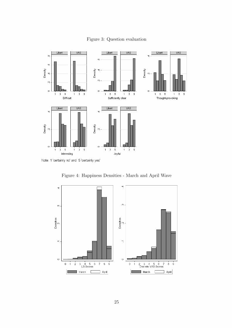
Figure 3: Question evaluation
Figure 4: Happiness Densities - March and April Wave
25

Figure 5: Happiness Densities - March Wave
26