In-flight calibration of SCIAMACHY’s polarization … · Patricia Liebing1,a, Matthijs...
25
Atmos. Meas. Tech., 11, 265–289, 2018 https://doi.org/10.5194/amt-11-265-2018 © Author(s) 2018. This work is distributed under the Creative Commons Attribution 3.0 License. In-flight calibration of SCIAMACHY’s polarization sensitivity Patricia Liebing 1,a , Matthijs Krijger 2,b , Ralph Snel 2,c , Klaus Bramstedt 1 , Stefan Noël 1 , Heinrich Bovensmann 1 , and John P. Burrows 1 1 Institute of Environmental Physics (IUP), University of Bremen, Bremen, Germany 2 SRON Netherlands Institute for Space Research, Sorbonnelaan 2, 3584 CA Utrecht, the Netherlands a now at: Leiden Observatory, 2300 RA Leiden, the Netherlands b now at: Earth Space Solutions, Utrecht, the Netherlands c currently at: TNO, Stieltjesweg 1, 2628 CK Delft, the Netherlands Correspondence: Patricia Liebing ([email protected]) Received: 1 June 2017 – Discussion started: 31 July 2017 Revised: 3 November 2017 – Accepted: 20 November 2017 – Published: 15 January 2018 Abstract. This paper describes the in-flight calibration of the polarization response of the SCIAMACHY polariza- tion measurement devices (PMDs) and a selected region of its science channels. With the lack of polarized calibration sources it is not possible to obtain such a calibration from dedicated calibration measurements. Instead, the earthshine itself, together with a simplified radiative transfer model (RTM), is used to derive time-dependent and measurement- configuration-dependent polarization sensitivities. The re- sults are compared to an instrument model that describes the degradation of the instrument as a result of a slow buildup of contaminant layers on its elevation and azimuth scan mir- rors. This comparison reveals significant differences between the model prediction and the data, suggesting an unforeseen change between on-ground and in-flight calibration in at least one of the polarization-sensitive components of the optical bench. The possibility of mechanisms other than scan mirror contamination contributing to the degradation of the instru- ment will be discussed. The data are consistent with a po- larization phase shift occurring in the beam split prism used to divert the light coming from the telescope to the different channels and polarization measurement devices. The exten- sion of the instrument degradation model with a linear re- tarder enables the determination of the relevant parameters to describe this phase shift and ultimately results in a significant improvement of the polarization measurements as well as the polarization response correction of measured radiances. 1 Introduction SCIAMACHY (Bovensmann et al., 1999) was a passive spectrometer onboard ESA’s Envisat platform, operational between 2002 and 2012. Spectra of the radiance upwelling at the top of the atmosphere in nadir, limb and occultation geometries as well as of the extraterrestrial solar irradiance were measured by SCIAMACHY. The uncalibrated level 0 data are transformed by applying the instrument response functions, obtained during preflight and in-flight calibration, to the radiance, irradiance and reflectance. Measurements be- tween 214 and 1750 nm were contiguously recorded in six channels at wavelength-dependent spectral resolutions be- tween 0.2 and 1.5 nm. In addition, there were two channels with bands around 2.0 and 2.3 μm and spectral resolutions around 0.2 nm and seven polarization measurement devices, PMDs. The latter were broadband detectors at selected wave- lengths. Combined with the spectral channels they were used to determine the polarization of the upwelling radiation. The resulting radiance, irradiance and reflectance data products were used to derive column amounts and concentrations of atmospheric trace gases and aerosol and cloud data prod- ucts. The accuracy of these data products depends critically on that of the measured spectra, i.e., the absolute magnitude of the radiometric signals and their spectral shape. There- fore, it is vital to obtain a highly accurate characterization of the instrument response functions to unpolarized and polar- ized light, both from on-ground measurements and in-flight measurements. SCIAMACHY is equipped with scan mirrors to reflect the light from nadir or limb line of sights into the Published by Copernicus Publications on behalf of the European Geosciences Union.
Transcript of In-flight calibration of SCIAMACHY’s polarization … · Patricia Liebing1,a, Matthijs...
Atmos. Meas. Tech., 11, 265–289, 2018https://doi.org/10.5194/amt-11-265-2018© Author(s) 2018. This work is distributed underthe Creative Commons Attribution 3.0 License.
In-flight calibration of SCIAMACHY’s polarization sensitivityPatricia Liebing1,a, Matthijs Krijger2,b, Ralph Snel2,c, Klaus Bramstedt1, Stefan Noël1, Heinrich Bovensmann1, andJohn P. Burrows1
1Institute of Environmental Physics (IUP), University of Bremen, Bremen, Germany2SRON Netherlands Institute for Space Research, Sorbonnelaan 2, 3584 CA Utrecht, the Netherlandsanow at: Leiden Observatory, 2300 RA Leiden, the Netherlandsbnow at: Earth Space Solutions, Utrecht, the Netherlandsccurrently at: TNO, Stieltjesweg 1, 2628 CK Delft, the Netherlands
Correspondence: Patricia Liebing ([email protected])
Received: 1 June 2017 – Discussion started: 31 July 2017Revised: 3 November 2017 – Accepted: 20 November 2017 – Published: 15 January 2018
Abstract. This paper describes the in-flight calibration ofthe polarization response of the SCIAMACHY polariza-tion measurement devices (PMDs) and a selected region ofits science channels. With the lack of polarized calibrationsources it is not possible to obtain such a calibration fromdedicated calibration measurements. Instead, the earthshineitself, together with a simplified radiative transfer model(RTM), is used to derive time-dependent and measurement-configuration-dependent polarization sensitivities. The re-sults are compared to an instrument model that describes thedegradation of the instrument as a result of a slow buildupof contaminant layers on its elevation and azimuth scan mir-rors. This comparison reveals significant differences betweenthe model prediction and the data, suggesting an unforeseenchange between on-ground and in-flight calibration in at leastone of the polarization-sensitive components of the opticalbench. The possibility of mechanisms other than scan mirrorcontamination contributing to the degradation of the instru-ment will be discussed. The data are consistent with a po-larization phase shift occurring in the beam split prism usedto divert the light coming from the telescope to the differentchannels and polarization measurement devices. The exten-sion of the instrument degradation model with a linear re-tarder enables the determination of the relevant parameters todescribe this phase shift and ultimately results in a significantimprovement of the polarization measurements as well as thepolarization response correction of measured radiances.
1 Introduction
SCIAMACHY (Bovensmann et al., 1999) was a passivespectrometer onboard ESA’s Envisat platform, operationalbetween 2002 and 2012. Spectra of the radiance upwellingat the top of the atmosphere in nadir, limb and occultationgeometries as well as of the extraterrestrial solar irradiancewere measured by SCIAMACHY. The uncalibrated level 0data are transformed by applying the instrument responsefunctions, obtained during preflight and in-flight calibration,to the radiance, irradiance and reflectance. Measurements be-tween 214 and 1750 nm were contiguously recorded in sixchannels at wavelength-dependent spectral resolutions be-tween 0.2 and 1.5 nm. In addition, there were two channelswith bands around 2.0 and 2.3 µm and spectral resolutionsaround 0.2 nm and seven polarization measurement devices,PMDs. The latter were broadband detectors at selected wave-lengths. Combined with the spectral channels they were usedto determine the polarization of the upwelling radiation. Theresulting radiance, irradiance and reflectance data productswere used to derive column amounts and concentrations ofatmospheric trace gases and aerosol and cloud data prod-ucts. The accuracy of these data products depends criticallyon that of the measured spectra, i.e., the absolute magnitudeof the radiometric signals and their spectral shape. There-fore, it is vital to obtain a highly accurate characterization ofthe instrument response functions to unpolarized and polar-ized light, both from on-ground measurements and in-flightmeasurements. SCIAMACHY is equipped with scan mirrorsto reflect the light from nadir or limb line of sights into the
Published by Copernicus Publications on behalf of the European Geosciences Union.

266 P. Liebing et al.: In-flight polarization calibration
telescope and then further towards grating spectrometers andphotodiode detectors. The degradation of the scan mirrorscan be modeled with a thin, slowly growing layer of contami-nant on top of their oxidized aluminum surfaces. In-flight cal-ibration measurements for SCIAMACHY were carried outregularly with unpolarized sources, mainly the Sun, and fordifferent scan mirror configurations and positions. These datahave been analyzed with the so-called scan mirror modelwhich, by applying the Fresnel equations for layered surfacesto these specific measurement configurations, determined therefractive indices and thicknesses of the contaminant on eachof the two scan mirrors (Krijger et al., 2014). Indeed, a ma-jor part of the observed instrumental throughput degradationin the UV, and its scan angle dependence, can be explainedby the contamination of the scan mirrors. The remaining partis attributed to the degradation of the optical bench module(OBM), which comprises all elements of the optical train be-hind the instrument slit.
The spectrometer grating and also the scan mirrors andother optical components along the light path are polariza-tion sensitive, meaning that their optical properties dependpartially on the polarization of the incident light. The po-larization sensitivity of the instrument as a whole has beenmeasured on the ground (Gottwald and Bovensmann, 2011)and found to be substantial, on the order of 20 % or more,over large wavelength ranges. The measured polarization val-ues, obtained from the combination of PMD and sciencechannel measurements, can be used to correct the signal ofthe SCIAMACHY science channels. For this correction tobe effective, both the polarization and the polarization re-sponse have to be known with sufficient accuracy. Measuredpolarization and reflectance values in the visible and near-infrared range have been compared to POLDER data andfound to be within the expected range for selected geome-tries in nadir (Tilstra and Stammes, 2007, 2010). Limb polar-ization data on the other hand differed systematically fromradiative transfer model (RTM) results (Liebing et al., 2013),an effect which is largest in the UV and decreases towardslonger wavelengths. Of importance is the observation that,even though the data show a significant drift over time, adifference between in-flight and preflight measurements isalready present early in the mission. These findings implythat there were either unidentified systematic errors in the on-ground calibration or perhaps a sudden change in the polar-ization calibration parameters shortly after launch, followedby an in-flight degradation of polarization-sensitive compo-nents. Due to the variation in the observation geometry – andtherefore in the polarization – with latitude and season, er-rors in the polarization determination or correction may leadto latitudinally and seasonally dependent systematic errors inthe derived atmospheric trace gas concentrations. Moreover,long-term degradation effects may consequently lead to driftsin the data if not appropriately accounted for.
Recently, the on-ground calibration data have been re-analyzed, making use of the scan mirror model for SCIA-
MACHY (Krijger et al., 2014). The application of this modelfor uncontaminated mirrors during the on-ground calibrationcampaign enables the separation of the radiance and polariza-tion sensitivities of the scan mirrors from that of the OBM.The knowledge of the OBM polarization response can thenbe combined with that on the mirror contamination in spacederived from the in-flight calibration measurements. The ap-plication of the model to nadir and limb measurement con-figurations yields a prediction of the time-dependent behav-ior of in-flight polarization sensitivities for limb and nadirobservations.
The aim of this paper is to devise a method for the directin-flight calibration of the polarization response which en-ables a validation of the scan mirror model and its derived pa-rameters as well as a correction for the suspected on-groundto in-flight change. Furthermore, an investigation of this on-ground to in-flight change leads to its most likely culprit: apolarization phase shift induced in the beam split prism thatis used to separate the almost completely polarized beamsfor the PMDs from the partially polarized beams for the sci-ence detectors. Such a phase shift can be modeled with anextension to the scan mirror model that includes a linear re-tarder and thus modifies the OBM polarization sensitivitiesas measured on the ground.
A polarized calibration source is necessary in order to de-rive the in-flight polarization sensitivities. As the Sun and on-board calibration sources are unpolarized, the only availablepolarized calibration source is the earthshine itself. By ex-ploiting the relationship between depolarization and intensityat fixed wavelength and viewing geometry, data points withknown polarization can be selected and sampled in order toobtain the polarization sensitivities. The information avail-able in the data permits this to be done only for the PMDsand for a particular feature in SCIAMACHY’s science chan-nel at around 350 nm. The statistical nature of this approachmitigates errors arising from the underlying assumptions to acertain degree; the remaining errors are to be estimated fromthe systematic variation of those assumptions. The results ob-tained in the UV and, partially, visible (VIS) regions prove tobe accurate enough to deduce from them the parameters ofthe instrumental phase shift and its possible cause. This in-vestigation may also be relevant in view of other instrumentswhose design follows a similar principle, such as the GOMEseries on the ERS-2 and MetOp satellites.
The structure of this article is as follows: in Sect. 2, first thepolarization formalism used here is introduced, including theMueller matrix approach and the description of the polariza-tion coordinate frame. Next, the SCIAMACHY polarizationmeasurements are explained in detail. Section 3 explains thecalibration strategy and presents the results. The interpreta-tion of the results in terms of an on-ground to in-flight changein the OBM and possibly its further degradation is presentedin Sect. 4. This section also contains a discussion on impli-cations regarding the status of the instrument before and af-
Atmos. Meas. Tech., 11, 265–289, 2018 www.atmos-meas-tech.net/11/265/2018/
P. Liebing et al.: In-flight polarization calibration 267
ter launch and on the applicability of the scan mirror model.Conclusions are presented in Sect. 5.
2 Polarization formalism and measurements
Throughout this paper, we employ the Mueller matrix for-malism to describe the instruments sensitivity to polarizedlight. The formalism, frame definitions and application toSCIAMACHY are presented in this section together with adescription of the polarization measurement approach.
2.1 Mueller matrix formalism and polarization frame
Formally, the measured signal of any given polarization-sensitive instrument is the first element of the Stokes vec-tor resulting from the product of the incoming Stokes vec-tor I = (I,Q,U,V )T with the 4 × 4 Mueller matrix that de-scribes its modification by the optical elements inside the in-strument:
S0 = [M · I ]0. (1)
The Stokes vector components are combinations of the in-tensities I with different polarization planes with respect toa given reference frame:
I = I‖+ I⊥ , Q= I‖− I⊥ , U = I45◦ − I−45◦ ,
V = IR − IL . (2)
The linear polarization is defined by the Q and U com-ponents; V is the circular polarization component. Of-ten, the Stokes vector is given in relative terms, i.e., I =I (1,q,u,v)T , where the second to fourth components cantake values between −1 and 1 and the total degree of polar-ization is defined as
p ≡
√q2+ u2+ v2 ≤ 1. (3)
The Stokes vector frame is defined by choosing the parallel(‖) axis. The perpendicular (⊥) axis is then naturally given,while for the ±45◦ direction as well as the left (L) and right(R) handedness of the circular polarization a sense of orien-tation needs to be defined. Here, the sense of orientation isgiven by looking into the travel direction of the light, i.e.,towards the instrument. A positive rotation is defined to beclockwise, i.e., left-handed.
The elements of the Mueller matrix can be interpreted inthe following way:M11 is the optical throughput for unpolar-ized light, i.e., I = (I,0,0,0)T . The other diagonal elementsMii describe the transfer efficiency for a given input Stokesvector component (Q for i = 2, U for i = 3, V for i = 4)to the output Stokes vector, while the non-diagonal elementsstand for the crosstalk between different Stokes vector com-ponents. The instrument Mueller matrix itself is the productof the Mueller matrices of its individual components. The
Mueller matrix needs to be given in the same reference frameas the Stokes vector and, if necessary, reference frames forindividual components have to be transformed to this partic-ular reference frame.
Since only the first component of the signal Stokes vectorS0 ≡ S is being measured, only the first row of the instru-ment Mueller matrix is needed for calibration of the detectorsignal:
S = IM11(1,µ2,µ3,µ4)(1,q,u,v)T , (4)
where the µi =M1i/M11 are the normalized Mueller matrixelements (MMEs). Note that, if the end-to-end Mueller ma-trix is derived from a combination of individual matrices, allbut the last one of those still have to be known completely.
For SCIAMACHY, the Stokes frame for the measured at-mospheric polarization is defined with respect to the localmeridional plane, the plane spanned by the line of sight andthe local zenith. Parallel polarization, i.e., q =+1, is givenwhen the polarization lies in this plane. Positive 45◦ polar-ization u=+1 is defined for the polarization plane which isrotated clockwise by 45◦ from the parallel direction, whenlooking along the line of sight into the instrument. For cali-bration purposes and within the scan mirror model, anotherframe definition is applied. The end-to-end Mueller matrixor Stokes vectors can easily be transformed between thesedifferent frames. In this paper we work entirely with the at-mospheric polarization, and, to avoid confusion, we chooseto give the end-to-end Mueller vector in the atmospheric po-larization frame.
2.2 The scan mirror model
The details of the scan mirror model and its application toSCIAMACHY are described in Krijger et al. (2014). Essen-tially, the instrument is separated into a scan module con-sisting of one or several scan mirrors and the optical benchmodule which comprises everything else, i.e.,
S = IMOBM11 µOBMM(α)(1,q,u,v)T . (5)
Here, µOBM is the first row vector of the normalized OBMMueller matrix, MOBM
11 is the unpolarized radiance responseof the OBM and M(α) is the scan mirror Mueller matrixwhich depends on the incidence angle(s) α. Depending on thescan mirror configuration in use (one or more mirrors withreflection planes at an angle), it can be the product of severalMueller matrices appropriately transformed to match theirrespective coordinate systems. The Mueller matrix of any ofthe scan mirrors can be calculated from the Fresnel equa-tions, possibly taking into account multiple layers of mate-rial and knowing their complex refractive indices and thick-nesses. The separation of the instrument into these two mod-ules enables two separate calibration steps: on the ground,the calibration data which were obtained with particular scanmirror configurations can be modeled with uncontaminated
www.atmos-meas-tech.net/11/265/2018/ Atmos. Meas. Tech., 11, 265–289, 2018

268 P. Liebing et al.: In-flight polarization calibration
mirrors to yield the OBM Mueller vector (Krijger, 2017).In-flight, the calibration measurements with a stable, unpo-larized source (the Sun or the internal white light source)can be used to determine the thickness and refractive indexof a contaminant layer on each of the involved scan mir-rors, assuming a fixed OBM. Realistically, the limited in-formation contained in the combination of calibration mea-surements used only allows for the determination of a sin-gle wavelength-dependent refractive index which is constantin time and the time-dependent thicknesses on each of thescan mirrors. Additionally, an extra factor, called “M-factor”,is introduced to indicate the degradation of the unpolarizedOBM response. However, the separation of mirror and OBMdegradation given the information contained in the calibra-tion measurements is not entirely unambiguous – in the sensethat to some degree both can describe the unpolarized cali-bration measurements equally well.
2.3 Nadir and limb scans
The relevant measurements discussed here are nadir and limbreflectance and polarization measurements. SCIAMACHYperforms both observation modes in an alternating sequence.Envisat’s Sun-synchronous orbit crosses the descending nodeat 10:00 local time, such that the Sun is always to the left ofthe flight direction, with a minimum solar zenith angle (SZA)of about 20◦.
A nadir scan is carried out by pointing the ESM (elevationscan module) mirror toward the surface and then continu-ously scanning from left to right, thereby covering elevationangles up to 32◦ and a total swath width of 960 km. Duringthe scan, the detector signal is read out several times. Theintegration time depends on wavelength and SZA. The dataconsidered here are all selected to have integration times of0.25 s or less, such that 16 readouts per scan are available.The ground pixel size thus amounts to 60 km across track asdetermined by the integration time and 30 km along track asdetermined by the length of the instrument slit of 1.8◦ and themotion of the spacecraft. The scan takes 4 s and is followedby a fast backward scan of 1 s. This sequence is typically re-peated 13 times before switching to a limb scan.
During a limb scan, the ASM (azimuth scan module) mir-ror is pointed approximately into the flight direction, to-ward the limb of Earth’s atmosphere. The projection of theinstrument slit is parallel to the horizon, providing an in-stantaneous field of view of about 103 km horizontally and2.6 km vertically. The light is reflected off the ASM mirrortoward the ESM mirror which is set at an elevation angleof about 63◦. The reflection planes of both mirrors are atan angle to each other. In the scan mirror model, this angleis properly accounted for by rotating the respective coordi-nate systems. The ASM mirror performs a horizontal scanof about ±10◦ around the flight direction at a fixed ESM el-evation angle, starting approximately 3 km below the hori-zon. The horizontal scan takes 1.5 s, again covering a swath
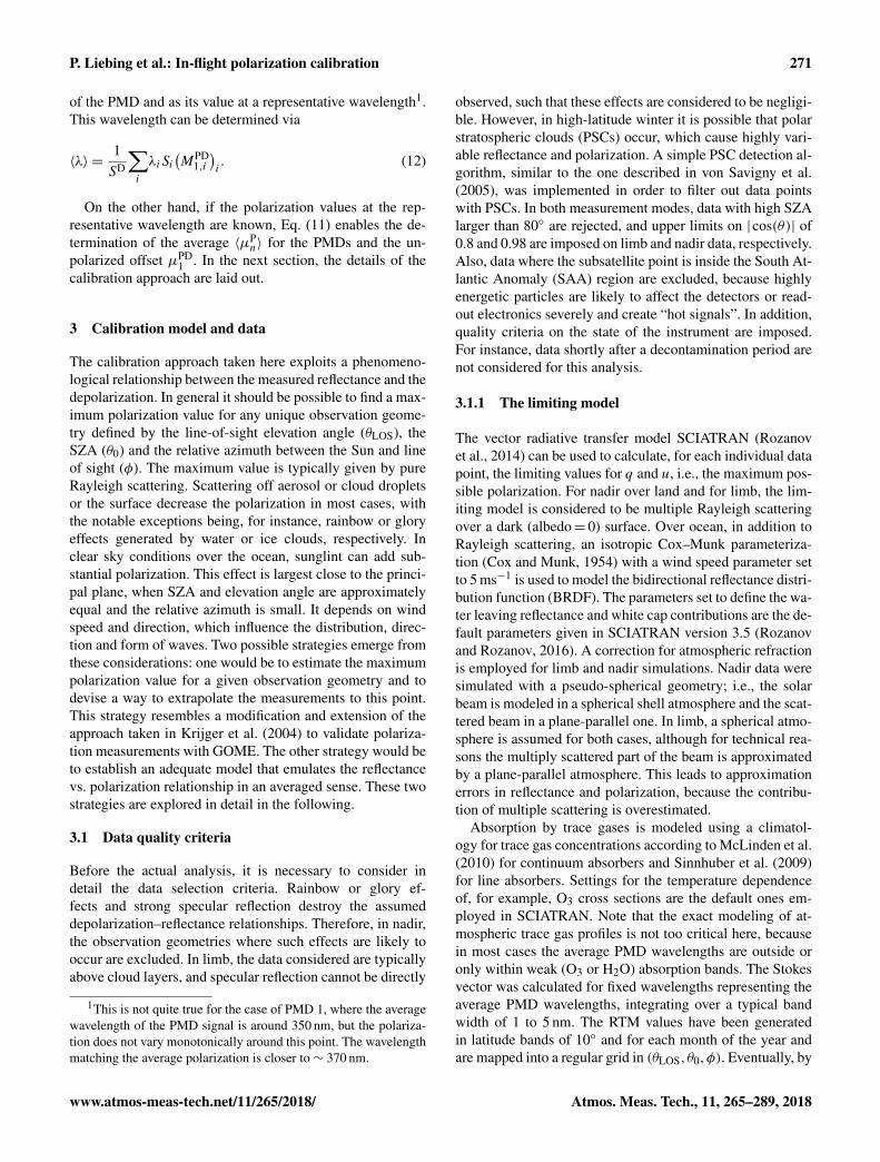
of 960 km. After the scan, the ESM elevation angle is in-creased by about 3.3 km and the horizontal scan proceeds inthe other direction. Between 29 and 34 such horizontal scansare performed in one sequence, thus covering altitudes be-tween about −3 and 93 km or higher. After the last scan,another ESM elevation step to an altitude of about 250 kmis executed, and a dark measurement is performed for thelast 1.5 s of the sequence. This dark measurement is typi-cally used to correct the detector signals for potentially orbit-phase-dependent dark current conditions. During a horizon-tal scan, the typical integration time is 0.375 s, resulting infour radiance profiles per limb scan. With Envisat flying atan altitude of about 790 km, the tangent points of a limb scanare about 3300 km ahead of the subsatellite point. The mea-surement sequence is designed such that about 7 min after alimb scan a nadir sequence is performed whose ground pixelsoverlap with the limb tangent points, thus enabling stereo-scopic measurements. In Fig. 1, the scan mirror configura-tions and viewing geometries for the nadir and limb observa-tion modes are depicted on the left and right, respectively. Inthe nadir configuration, the instrument slit is oriented alongthe flight direction and therefore perpendicular to the merid-ional plane, which lies in the scan direction. In limb, the pro-jection of the slit is along the horizon and therefore againperpendicular to the plane connecting the line of sight and lo-cal zenith or tangent point. Therefore, in both cases, q =−1when the polarization direction (in the atmospheric Stokesframe) is along the instrument slit projection.
The true light path along the line of sight of a limb mea-surement depends critically on wavelength and the scene ob-served. Topography and horizontally inhomogeneous cloudor aerosol layers make observations in the troposphere highlyvariable. However, in the stratosphere, under relatively stableaerosol conditions, reflectance measurements are quite suit-able for systematic studies. A possible issue persists in thecontamination with spatial stray light, either from the Sunor from bright scenes below the tangent altitude. The mea-surements considered here are always done with the relativeazimuth angle with the Sun larger than 20◦, thereby minimiz-ing the possible contamination with solar stray light. Earth-shine stray light, however, is clearly visible at tangent heights(THs) above 40 km and becomes dominant at altitudes largerthan about 60 km. Below 40 km, its contribution is not ex-pected to be larger than a few per cent.
Reflectances are obtained by normalizing limb or nadir ra-diances with the solar irradiance, which is measured once perday using a combination of a diffuser on the backside of theESM and the ASM mirror.
2.4 SCIAMACHY polarization measurements
Generically, polarization can be measured by modifying theMueller matrix in Eq. (4) such that the measured signal be-comes sensitive to different linear combinations of the Stokesvector components. In order to derive all components unam-
Atmos. Meas. Tech., 11, 265–289, 2018 www.atmos-meas-tech.net/11/265/2018/

P. Liebing et al.: In-flight polarization calibration 269
x
y
z
ightF l direction
adir N
T elescope
ESMx
y
z
direction
ASM
ESM
(a) (b)
ightF l
T elescope
adir N
Figure 1. Sketch of the scan mirror configuration and viewing geometry during nadir (a) and limb (b) observations. In nadir mode, the ESMmirror is rotated to achieve a scan across track. In limb mode, the ASM mirror is rotated to achieve a scan across the flight direction, whilethe ESM mirror performs small steps to select a specific tangent height. Their reflection planes are rotated with respect to each other.
biguously, at least four independent measurements per wave-length have to be carried out. The circular polarization com-ponent is typically negligible in atmospheric polarization, re-ducing the minimum number of required measurements tothree. These can be either carried out sequentially, or, as inthe case of SCIAMACHY, simultaneously by employing abeam splitter. The beam split device in SCIAMACHY is theso-called “predisperser prism” which is located right after thetelescope. It serves two purposes: the first is to spatially sepa-rate different spectral ranges of the incoming light in order tofacilitate their diversion into SCIAMACHY’s eight spectralchannels. The second purpose is to split off a small fractionof the beam through internal reflection at the Brewster angleand thus generate an almost fully polarized beam which is di-rected towards the polarization measurement devices, a set ofphotodiode detectors sampling at a rate of 40 Hz and integrat-ing over relatively wide spectral regions (100 to 200 nm) thatroughly correspond to the central part of each of the mainscience channels. Figure 2 gives a schematic overview ofthe measurement principle. After passing the scanner mod-ule depicted on the left, the light enters the telescope withthe instrument slit. The incidence on the first surface of thepredisperser prism is nominal, and thus no spectral diversionoccurs inside it. Most of the light exits on the opposite side,which is tilted, and is refracted toward the science channels.The remaining part of the beam undergoes internal reflectionunder the Brewster angle, after which it is almost fully po-larized with its polarization direction pointing into the paper(indicated by the crossed circle), i.e., parallel to the instru-ment slit. After another internal reflection it exits the prismand is refracted towards the PMDs.
Table 1 lists the PMDs used for this investigation and theirrelevant properties. The average wavelength given there isapproximate, since it depends in detail on the shape of themeasured spectrum. Also given in this table are the sensitiv-ity to unpolarized light relative to that of the science chan-nel (〈M1〉
PD) and the three components of the OBM Muellervector, which are all spectrally averaged. PMD 7 is specialin the sense that its signal is not split off at the predisperser
prism, but rather at the location of channel 5, and the 45◦ po-larization is obtained by employing a polarization filter. Itsspectral range is nearly identical with that of PMD 4. WhilePMD 7 has its largest sensitivity to light polarized at 45◦,i.e., µ3 ≈ 1, the other PMDs are mostly sensitive to light po-larized parallel to the direction of the instrument slit; henceµ2 ≈−1. Take note of the relatively large sensitivity to cir-cular polarization, which in fact is unexpected given the de-sign of the PMDs and poses a serious problem to the SCIA-MACHY polarization measurements. Even though the atmo-spheric radiance is not circularly polarized, the scan mirrorswill convert 45◦ linearly polarized light to circularly polar-ized light. The end-to-end Mueller vector of the PMDs thuscontains a large, unwanted sensitivity to 45◦ polarization.A similar effect was discovered for the science channels aswell. Since it was originally deemed sufficient to determineonly q and to correct the science channel radiance for thisStokes component only, a measurement of the u componentwas not foreseen. This is only possible for the wavelengthregion around 850 nm, where both PMD 4 and 7 are avail-able. For the other regions, assumptions on the relationshipbetween q and u or on the value of u itself have to be madein order to be able to derive q and to correct the measuredsignal adequately.
The polarization is determined by equating the synchro-nized and integrated (over the exposure time of the sciencechannel) PMD signal with the calibrated science channel sig-nal scaled with the PMD response and integrated over thePMD spectral band:
SP= µPD
1 ·∑i
SDi M
PD1,i
1+µP2,iq +µ
P3,iu
1+µD2,iq +µ
D3,iu
, with (6)
MPD1,i =
MP11,i
MD11,i
. (7)
The sum goes over all pixels in the relevant spectral range;the superscripts P and D indicate the PMD and science detec-
www.atmos-meas-tech.net/11/265/2018/ Atmos. Meas. Tech., 11, 265–289, 2018

270 P. Liebing et al.: In-flight polarization calibration
Optical bench module (OBM)Scanner module
Sciencechannels
PMDs
Telescope
Predisperserprism
ESM
ASM
Nad
ir
Limb
Slit
!"
ASMC
onta
min
ant
Con
tam
inan
t
(a) (b)
Figure 2. Sketch of the measurement principle of SCIAMACHY. The left part indicates the scanner module with different mirror config-urations, with their optical properties described by the scan mirror model. The scan mirrors can contain a contaminant layer. On the right,the optical bench module is depicted, which includes the telescope, the predisperser prism, and the science channel and PMD detectors. Thecrossed circle indicates the polarization direction of the PMD beam after internal reflection inside the prism (into the paper). The opticaltrain between the predisperser prism and the PMD and science channel detectors has been omitted; for details, we refer to Gottwald andBovensmann (2011).
Table 1. SCIAMACHY PMDs, their spectral range, average wavelength, reference wavelength, corresponding SCIAMACHY science chan-nel and spectrally averaged OBM Mueller matrix elements for the PMDs.
PMD Range 〈λ〉 λC Channel 〈M1〉PD
〈µ2〉 〈µ3〉 〈µ4〉(nm) (nm)
1 305–385 352 370 2 0.17 −0.86 −0.004 −0.482 430–550 484 480 3 0.02 −0.92 0.013 −0.303 590–720 656 655 4 0.016 −0.94 0.013 −0.204 780–920 852 850 5 0.035 −0.95 0.018 −0.115 1400–1750 1570 1555 6 0.099 −0.97 0.005 00.117 780–920 854 850 5 0.07 0.10 0.94 0.33
tors, respectively. The µP,Dn,i are the end-to-end Mueller vec-
tor elements and vary with observation mode and scan angle.The factor µPD
1 is an additional in-flight calibration factorthat accounts for calibration offsets in the relative PMD toscience channel response to unpolarized light. Assuming thatthe polarization and the polarization sensitivity varies suffi-ciently slowly with wavelength, this equation can be furthersimplified:
SP= µPD
1 ·∑i
SDi M
PD1,i
1+〈µP2〉q +〈µ
P3〉u
1+〈µD2 〉q +〈µ
D3 〉u
. (8)
The quantities in the angular brackets are now wavelengthindependent and refer to the intensity-weighted spectral av-erage of the polarization sensitivities:
〈µP,Dn 〉 =
1SD
∑i
SDi M
PD1,i µ
P,Dni , n= 2,3 , (9)
with
SD=
∑i
SDi M
PD1,i . (10)
The term SD is also called the “virtual sum” and describesthe expected PMD signal for zero polarization, given the sci-ence channel signal and the relative detector responses. WithEq. (10) a polarization signal, P , can be defined as the ratioof the PMD signal to the virtual sum,
P ≡ µPD1SP
SD ≈1+〈µP
2〉q +〈µP3〉u
1+〈µD2 〉q +〈µ
D3 〉u
, (11)
which depends on polarization only.Given known calibration constants and a relationship be-
tween q and u, or a known value for u, Eqs. (6) or (11) canbe solved and result in a value for q which can be interpretedboth as the signal-weighted average over the spectral width
Atmos. Meas. Tech., 11, 265–289, 2018 www.atmos-meas-tech.net/11/265/2018/
P. Liebing et al.: In-flight polarization calibration 271
of the PMD and as its value at a representative wavelength1.This wavelength can be determined via
〈λ〉 =1SD
∑i
λiSi(MPD
1,i)i. (12)
On the other hand, if the polarization values at the rep-resentative wavelength are known, Eq. (11) enables the de-termination of the average 〈µP
n〉 for the PMDs and the un-polarized offset µPD
1 . In the next section, the details of thecalibration approach are laid out.
3 Calibration model and data
The calibration approach taken here exploits a phenomeno-logical relationship between the measured reflectance and thedepolarization. In general it should be possible to find a max-imum polarization value for any unique observation geome-try defined by the line-of-sight elevation angle (θLOS), theSZA (θ0) and the relative azimuth between the Sun and lineof sight (φ). The maximum value is typically given by pureRayleigh scattering. Scattering off aerosol or cloud dropletsor the surface decrease the polarization in most cases, withthe notable exceptions being, for instance, rainbow or gloryeffects generated by water or ice clouds, respectively. Inclear sky conditions over the ocean, sunglint can add sub-stantial polarization. This effect is largest close to the princi-pal plane, when SZA and elevation angle are approximatelyequal and the relative azimuth is small. It depends on windspeed and direction, which influence the distribution, direc-tion and form of waves. Two possible strategies emerge fromthese considerations: one would be to estimate the maximumpolarization value for a given observation geometry and todevise a way to extrapolate the measurements to this point.This strategy resembles a modification and extension of theapproach taken in Krijger et al. (2004) to validate polariza-tion measurements with GOME. The other strategy would beto establish an adequate model that emulates the reflectancevs. polarization relationship in an averaged sense. These twostrategies are explored in detail in the following.
3.1 Data quality criteria
Before the actual analysis, it is necessary to consider indetail the data selection criteria. Rainbow or glory ef-fects and strong specular reflection destroy the assumeddepolarization–reflectance relationships. Therefore, in nadir,the observation geometries where such effects are likely tooccur are excluded. In limb, the data considered are typicallyabove cloud layers, and specular reflection cannot be directly
1This is not quite true for the case of PMD 1, where the averagewavelength of the PMD signal is around 350 nm, but the polariza-tion does not vary monotonically around this point. The wavelengthmatching the average polarization is closer to ∼ 370 nm.
observed, such that these effects are considered to be negligi-ble. However, in high-latitude winter it is possible that polarstratospheric clouds (PSCs) occur, which cause highly vari-able reflectance and polarization. A simple PSC detection al-gorithm, similar to the one described in von Savigny et al.(2005), was implemented in order to filter out data pointswith PSCs. In both measurement modes, data with high SZAlarger than 80◦ are rejected, and upper limits on |cos(θ)| of0.8 and 0.98 are imposed on limb and nadir data, respectively.Also, data where the subsatellite point is inside the South At-lantic Anomaly (SAA) region are excluded, because highlyenergetic particles are likely to affect the detectors or read-out electronics severely and create “hot signals”. In addition,quality criteria on the state of the instrument are imposed.For instance, data shortly after a decontamination period arenot considered for this analysis.
3.1.1 The limiting model
The vector radiative transfer model SCIATRAN (Rozanovet al., 2014) can be used to calculate, for each individual datapoint, the limiting values for q and u, i.e., the maximum pos-sible polarization. For nadir over land and for limb, the lim-iting model is considered to be multiple Rayleigh scatteringover a dark (albedo= 0) surface. Over ocean, in addition toRayleigh scattering, an isotropic Cox–Munk parameteriza-tion (Cox and Munk, 1954) with a wind speed parameter setto 5 ms−1 is used to model the bidirectional reflectance distri-bution function (BRDF). The parameters set to define the wa-ter leaving reflectance and white cap contributions are the de-fault parameters given in SCIATRAN version 3.5 (Rozanovand Rozanov, 2016). A correction for atmospheric refractionis employed for limb and nadir simulations. Nadir data weresimulated with a pseudo-spherical geometry; i.e., the solarbeam is modeled in a spherical shell atmosphere and the scat-tered beam in a plane-parallel one. In limb, a spherical atmo-sphere is assumed for both cases, although for technical rea-sons the multiply scattered part of the beam is approximatedby a plane-parallel atmosphere. This leads to approximationerrors in reflectance and polarization, because the contribu-tion of multiple scattering is overestimated.
Absorption by trace gases is modeled using a climatol-ogy for trace gas concentrations according to McLinden et al.(2010) for continuum absorbers and Sinnhuber et al. (2009)for line absorbers. Settings for the temperature dependenceof, for example, O3 cross sections are the default ones em-ployed in SCIATRAN. Note that the exact modeling of at-mospheric trace gas profiles is not too critical here, becausein most cases the average PMD wavelengths are outside oronly within weak (O3 or H2O) absorption bands. The Stokesvector was calculated for fixed wavelengths representing theaverage PMD wavelengths, integrating over a typical bandwidth of 1 to 5 nm. The RTM values have been generatedin latitude bands of 10◦ and for each month of the year andare mapped into a regular grid in (θLOS,θ0,φ). Eventually, by
www.atmos-meas-tech.net/11/265/2018/ Atmos. Meas. Tech., 11, 265–289, 2018

272 P. Liebing et al.: In-flight polarization calibration
means of linear interpolation (in observation geometry only),a reference Stokes vector for the limiting RTM is availablefor each data point.
3.1.2 The extrapolation method
The data points for a given time period are now grouped ac-cording to the relevant scan angle (the position of the ESMmirror in nadir, the position of the ASM mirror for a fixedtangent height in limb) and in cells of (qRTM,uRTM) witha typical width of 0.01 in each direction (0.02 for limb),as a function of the RTM normalized average reflectanceR/RRTM at the PMD central wavelength. The subscript RTMstands for the appropriate limiting model. The average re-flectance is defined here as
R = π1N
∑i
I
I0|λi − λC | ≤ δλ, (13)
where I is the measured intensity and I0 the solar irradianceat each spectral pixel i within a window of width δλ aroundthe central wavelength λC given in Table 1. The width 1λis between 1 and 5 nm, depending on wavelength, and N isthe number of valid spectral points inside this window. The(qRTM,uRTM) cells are small enough that the viewing anglesin each vary only slightly. In each cell, the variation in thepolarization signal P with δR/RRTM = R/RRTM− 1 can befitted with a function of the following form:
f
(δR
RRTM
)= p0+
p1
1+p2δRRRTM
, (14)
with three fit parameters pi . This functional form is phe-nomenological but motivated by the expected behavior ofdepolarization induced by a single physical process, for in-stance the increase in surface albedo or of the aerosol con-centration of a fixed aerosol type. The depolarization of eachindividual process would then be governed by the parameterp2. In reality, multiple processes would contribute and causeconsiderable scatter. The underlying assumption here is thatthis scatter should decrease as the measured reflectance ap-proaches the RTM limit since each possible process can onlyhave a small effect, such that the data should converge to awell-defined slope. The polarization signal corresponding tothe maximum (RTM) polarization in the center of the cell isthen
P(0)= f (R = RRTM)≡ P(qRTM,uRTM)= p0+p1. (15)
For this fit, the reflectance is corrected for polarization withthe in-flight MMEs obtained from the scan mirror model andthe on-ground OBM Mueller vector for the correspondingwavelengths. Since in this step of the analysis the actual po-larization values for each data point data are not yet avail-able, the polarization values used in the correction are theRTM values themselves; i.e., each data point is corrected for
-1RTM R/R0 0.2 0.4 0.6 0.8 1 1.2 1.4 1.6 1.8
P
1.05
1.1
1.15
1.2
1.25
1.3
1.35
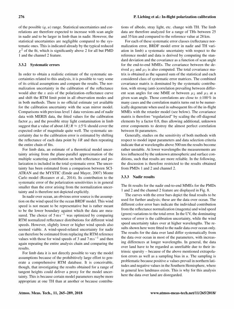
28 km≈Polarization signal, limb TH
) = (-0.26, -0.56)RTM,uRTM
(q°7≈PMD 1, ASM
°-5≈PMD 4, ASM
x21+p1
p0Pf =p +
Figure 3. Examples for the extrapolation method for limb, for afixed cell of (qRTM,uRTM). Blue points are for PMD 4, and redpoints are for PMD 1; the corresponding curves show the fittedfunctions.
the maximum polarization (qRTM,uRTM) at R = RRTM:
cPRTM =1
1+µ2qRTM+µ3uRTM. (16)
This means that the reflectance curve will be somewhat dis-torted towards the high reflectance tails. It has been veri-fied, though, that this has no influence on the estimate of thelimit towards the low reflectance values, where the correctionshould be closer to the truth.
In Fig. 3 the method is demonstrated for the case of PMD1 and PMD 4 in limb.
Note that for the examples in the figure the viewing ge-ometries for PMD 1 and 4 are not the same, despite the RTMpolarization values being the same. Also, in order to get asufficient amount and leverage of data for the fit, the datahave to be collected over the period of at least 1 month. Toavoid large extrapolation errors it is also vital to disregardcells where the minimum reflectance is too far away fromthe RTM limit, which happens very often at higher wave-lengths in nadir over land due to the contribution of surfacereflectance.
The fitted maximum polarization values fill a certain rangein the (q,u) plane which is determined by scan angle, scatter-ing geometries and the period of time integrated over. Here,this period is normally 1 calendar year, except for 2002, whenit starts only in August after the end of the commissioningphase, and for 2012, when the mission ended in April. A typ-ical example for the maximum polarization signal obtainedin nadir, 2004, is given in Fig. 4 for PMDs 1 and 4.
3.1.3 The lookup table method
The second approach is only realized for limb, where a largesimulation data set is available for a subset of the limb ob-servation geometries, comprising a range of aerosol profileswith different types, different cloud layers and types, and val-
Atmos. Meas. Tech., 11, 265–289, 2018 www.atmos-meas-tech.net/11/265/2018/

P. Liebing et al.: In-flight polarization calibration 273
Figure 4. Polarization signals for nadir (rainbow color code) vs. qRTM (x axis) and uRTM (y axis) over ocean in 2004 from the extrapolationmethod for PMD 1 (a, b), PMD 4 (c, d) and for two different ESM mirror positions during the nadir scan (a, c: east; b, d: west).
ues for the Lambertian albedo between 0 and 0.8. The detailson this simulation data set are already described in Liebinget al. (2013). In order to make these simulations applicable toall limb observation geometries, the simulated data are onceagain grouped according to observation geometry and av-eraged over a smaller subset of all scenarios, including allbut the highest values of stratospheric aerosol optical depth,which are unrealistic for the time period considered here. Anarithmetic average of q/qRTM (u/uRTM) of all scenarios isdetermined as a function of R/RRTM, where the subscriptRTM refers to the limiting RTM value for pure Rayleigh scat-tering. After smoothing, this average is mapped as a functionof qRTM (uRTM), such that for each PMD a two-dimensionallookup table (LUT) is available that delivers the depolariza-tion in each Stokes component as a function of its maximumRTM value. The approach is illustrated in Fig. 5 for PMDs 1and 4.
On the left side, the individual simulation points and theiraveraged values for a fixed TH (28 km) and fixed viewing ge-ometry are shown; the right side shows the two-dimensionalLUT built from a range of viewing geometries. From thisLUT, a value for (qLUT,uLUT) can be determined for eachdata point given in terms of (qRTM,uRTM,R/RRTM):
pLUT = pRTM
⟨p
pRTM
⟩(pRTM,R/RRTM) p = q,u. (17)
Also for this method, the reflectance values are corrected forpolarization using Eq. (16), except that here the RTM polar-ization values are replaced by the LUT polarization values,and an iteration step is performed to arrive at the final valuefor pLUT, given the polarization-corrected reflectance.
These data are again collected in cells of (qLUT,uLUT) andin bins of ASM mirror angle and tangent height and averagedover 1 year. Examples for the resulting distributions are givenon the right side of Fig. 6, together with the correspondingresults from the extrapolation method on the left, once againfor PMDs 1 and 4.
Comparing the extrapolation- and LUT-method values, itis evident that the sampling is much denser for the LUTmethod but that the range of (q,u) values covered is largerwith the extrapolation method – naturally because the extrap-olation method by definition always selects the maximumpossible polarization values. The LUT method is highly de-pendent on the assumptions used in the simulation of the dif-ferent scenarios, e.g., aerosol properties and profiles, and onthe scenario selections and averaging method applied to pre-pare the LUTs. Resulting calibration values may therefore beconsiderably model dependent. The extrapolation method onthe other hand is only marginally model dependent since thebasic mechanisms of Rayleigh and ocean surface scatteringare relatively well known and can be accurately computed.The potential pitfall lies in the assumption on how represen-tative the limiting polarization condition is and how well it
www.atmos-meas-tech.net/11/265/2018/ Atmos. Meas. Tech., 11, 265–289, 2018

274 P. Liebing et al.: In-flight polarization calibration
Figure 5. Example for the derivation of LUTs for the depolarization in limb geometry, TH≈ 28 km. (a) and (b) are for 375 nm (i.e., PMD1); (c) and (d) are for 850 nm (i.e, PMDs 4 and 7). On the left the depolarization for a fixed geometry is plotted vs. log(R/RRTM); on theright the 2D LUTs are shown as q/qRTM = f (qRTM, log(R/RRTM)) in a rainbow color scale.
Figure 6. Polarization signals for limb (rainbow color code) in 2004 vs. qRTM(LUT) (x axis) and uRTM(LUT) (y axis), TH≈ 28 km, from theextrapolation method (a, c) and the LUT method (b, d) for PMD 1 (a, b), PMD 4 (c, d) and for an ASM mirror angle of about +7◦.
Atmos. Meas. Tech., 11, 265–289, 2018 www.atmos-meas-tech.net/11/265/2018/

P. Liebing et al.: In-flight polarization calibration 275
Figure 7. Polarized end-to-end MMEs (µ2,3) for nadir (black: µ2;blue: µ3) and limb (red:µ2; green: µ3) calculated with the scanmirror model for August 2002. The MMEs are given in the atmo-spheric Stokes frame. The thick dashed vertical lines indicate thetwo spectral points used to build the polarization signal (see text).
can be reproduced by the fit with Eq. (14). For each indi-vidual case the resulting errors can hardly be estimated sincemany different effects may cancel or enhance each other, butthe comparison of the calibration parameters obtained by thetwo methods can provide a viable estimate of the typical un-certainties involved in this analysis.
3.2 The polarization feature at 350 nm
With the polarization signal as defined in Eq. (11), i.e., theratio of PMD to science channel signals, it is only possibleto derive the in-flight MMEs for the PMDs. There is no inde-pendent information on the science channel MMEs. A partic-ularly strong polarization feature in SCIAMACHY’s channel2, located at around 350 nm, opens up the possibility of de-riving information about the in-flight polarization sensitivityat this wavelength and as such enables a direct comparisonof science channel and PMD 1 behavior at almost the samewavelength. Figure 7 shows the polarized end-to-end MMEs(nadir and limb) for channel 2 as a function of wavelength.The properties of this feature indicate the presence of a so-called Wood’s anomaly (see, e.g., Maystre, 2012) of the grat-ing.
The feature at 350 nm was recognized as a potentialnoncompliance with respect to the instrument specification.However, the high throughput of this grating resulted inits selection nevertheless. Its sensitivity to polarization pro-vides independent information on the polarization responsein channel 2 but may contribute to noise or bias in trace gasretrievals if not perfectly accounted for.
The polarization-sensitive signal can be constructed bycomparing two relatively close spectral points with very dif-ferent polarization sensitivity. An obvious choice would bea point around 350 nm close to the minimum of µ2 and an-other one outside the feature at 370 nm where both MMEs
are relatively small. Points to the left of the feature are toosensitive to O3 concentrations and therefore not considered.The polarization signal is
P350
(R(370nm)
RRTM(370nm)
)≡
R(350nm)/R(370nm)RRTM(350nm)/RRTM(370nm)
= C
(R(370nm)
RRTM(370nm)
) 1+µ3502 q(350nm)+µ350
3 u(350nm)
1+µ3702 q(370nm)+µ370
3 u(370nm). (18)
The factor C accounts for a possible calibration offset as wellas a change in spectral slope between 350 and 370 nm withatmospheric or surface conditions. This is in contrast to thePMD to science channel polarization signal, which by defi-nition depends only on the polarization. For P350, this is onlythe case for the point where R(370nm)= RRTM(370nm),i.e., at the RTM limit. This also implies that the LUT methodcannot be applied for this polarization signal.
3.3 Derivation of in-flight Mueller matrix elements andtheir errors
3.3.1 Fit of end-to-end MMEs
The result of the previous analysis step are three-dimensionaldistributions of the polarization signal in (q,u,α), which canbe modeled as (see also Eq. 11)
P(u,q,α)= 〈µ1〉(α)1+〈µP2 〉(α)q +〈µ
P3 〉(α)u
1+〈µD2 〉(α)q +〈µD3 〉(α)u
, (19)
where α is the scan angle and
〈µi〉(α)= pi0+pi1α+pi2α2, pi2 ≡ 0 for limb. (20)
Due to the limited range of (q,u) values covered, it is notpossible to simultaneously fit all five MMEs. The aim is in-stead to fit the PMD parameters and the unpolarized scalefactor 〈µ1〉 in a linear fit. This is achieved by correcting thepolarization signal for the science channel contribution bysimply multiplying each cell value by a factor:
CD = 1+〈µD2 〉(α)qRTM,LUT+〈µD3 〉(α)uRTM,LUT. (21)
For the channel 2 feature µ350i corresponds to µPi , and the
µDi ’s are to be replaced by the MMEs at 370 nm, µ370i . The
RTM polarization values at 370 nm have to be used for thecorrection of the reflectance.
The fit is performed as a weighted least squares fit. Thefit parameters are the pij in Eq. (20). The statistical errors ofthe fit parameters and their correlations are determined by theextrapolation fit error (extrapolation method) or by the errorof the mean (LUT method) in each cell and the density andleverage of the 2D (q,u) distribution. Figure 4 can alreadygive an impression about the uneven distribution of data cellsfor different scan angles in nadir, and in Fig. 6 it should bepointed out that the limb data cover mostly only one quadrant
www.atmos-meas-tech.net/11/265/2018/ Atmos. Meas. Tech., 11, 265–289, 2018
276 P. Liebing et al.: In-flight polarization calibration
of the possible (q,u) range. Statistical uncertainties and cor-relations are therefore expected to increase with scan anglein nadir and to be larger in limb than in nadir. However, thestatistical uncertainties are negligible compared to the sys-tematic ones. This is indicated already by the typical reducedχ2 of the fit, which is significantly above 2 for all but PMD1 and the channel 2 feature.
3.3.2 Systematic errors
In order to obtain a realistic estimate of the systematic un-certainties related to this analysis, it is possible to vary someof its critical assumptions and compare the results. The nor-malization uncertainty in the calibration of the reflectancewould alter the x axis of the polarization–reflectance curveand shift the RTM limit point in all observation modes andin both methods. There is no official estimate yet availablefor the calibration uncertainty with the scan mirror model.Comparisons with previous level 1 data versions and of nadirdata with MERIS data, the fitted values for the calibrationfactor µ1 and the possible stray light contamination in limbsuggest that a value of about δR/R ≈±5% should cover theexpected order of magnitude quite well. The systematic un-certainty due to the calibration error is estimated by shiftingthe reflectance of each data point by δR and then repeatingthe entire chain of fits.
For limb data, an estimate of a theoretical model uncer-tainty arising from the plane-parallel approximation of themultiple scattering contribution on both reflectance and po-larization is included in the total systematic error. The uncer-tainty has been estimated from a comparison between SCI-ATRAN and the MYSTIC (Emde and Mayer, 2007) MonteCarlo model (Rozanov et al., 2014). Its contribution to thesystematic error of the polarization sensitivities is in generalsmaller than the error arising from the normalization uncer-tainty and is therefore not depicted explicitly.
In nadir over ocean, an obvious error source is the assump-tion on the wind speed for the ocean BRDF model. This windspeed is not meant to be representative but is rather meantto be the lower boundary against which the data are mea-sured. The choice of 5 ms−1 was optimized by comparingRTM normalized reflectance distributions for different windspeeds. However, slightly lower or higher wind speeds alsoseemed viable. A wind-speed-related uncertainty for nadircan therefore be estimated from replacing the RTM referencevalues with those for wind speeds of 3 and 7 ms−1 and thenagain repeating the entire analysis chain and comparing theresults.
For limb data it is not directly possible to vary the modelassumptions because of the prohibitively large effort to gen-erate a comprehensive RTM database. It is conceivable,though, that investigating the results obtained for a range oftangent heights could deliver a proxy for the model uncer-tainty. This is because certain model parameters maybe moreappropriate at one TH than at another or because contribu-
tions of albedo, stray light, etc. change with TH. The limbdata are therefore analyzed for a range of THs between 25and 35 km and compared to the reference value at 28 km.
For each of these systematic error classes (reflectance nor-malization error, BRDF model error in nadir and TH vari-ation in limb) a systematic uncertainty with respect to thereference model and data is derived by computing the stan-dard deviation and the covariance as a function of scan anglefor the end-to-end MMEs. The covariance between the de-rived µ2 and µ3 is also computed. The total covariance ma-trix is obtained as the squared sum of the statistical and eachconsidered class of systematic error matrices. The combinedcovariance matrix is dominated by the systematic contribu-tion, with strong (anti-)correlation prevailing between differ-ent scan angles for one MME or between µ2 and µ3 at agiven scan angle. Those correlations are close to ±100% inmany cases and the correlation matrix turns out to be numer-ically degenerate when used in subsequent fits of the in-flightMMEs with the retarder model (see below). The covariancematrix is therefore “regularized” by scaling the off-diagonalelements by a factor 0.8, thus allowing additional, unknownerror components to destroy the almost perfect correlationbetween fit parameters.
Generally, studies on the sensitivity of both methods withrespect to model input parameters and data selection criteriaindicate that at wavelengths above 500 nm the results becomerather unstable. At lower wavelengths the measurements areless influenced by the unknown atmospheric and surface con-ditions, such that results are more reliable. In the following,the discussion is therefore restricted to the results obtainedfrom PMDs 1 and 2 and channel 2.
3.3.3 Nadir results
The fit results for the nadir end-to-end MMEs for the PMDs1 and 2 and the channel 2 feature are displayed in Fig. 8.
The curves with the error bars depict the final results to beused for further analysis; these are the data over ocean. Thedifferent color error bars indicate the individual contributionfrom the reflectance normalization (magenta) and wind speed(green) variations to the total error. In the UV, the dominatingsource of error is the calibration uncertainty, while the windspeed uncertainty takes over at higher wavelengths. The re-sults shown here were fitted to the nadir data over ocean only.The results for the data over land differ systematically fromthe data over ocean in most of the parameters, with increas-ing differences at longer wavelengths. In general, the dataover land have to be regarded as unreliable due to their in-trinsic sparsity – because of the above mentioned extrapola-tion errors as well as a sampling bias in u. The sampling isproblematic because positive u values prevail in northern lati-tudes and negative values in the Southern Hemisphere, wherein general less landmass exists. This is why for this analysishere the data over land are disregarded.
Atmos. Meas. Tech., 11, 265–289, 2018 www.atmos-meas-tech.net/11/265/2018/

P. Liebing et al.: In-flight polarization calibration 277
Figure 8. Final results for end-to-end MMEs vs. ESM angle for nadir over ocean in 2004 from the extrapolation method. Rows: (a, d,g) channel 2 feature, (b, e, h) PMD 1, (c, f, i) PMD 2; columns: (a, b, c) 〈µ1〉, (d, e, f) 〈µP2 〉 and (g, h, i) 〈µP3 〉. Black data points are theresults with total errors; magenta and green error bars indicate the contribution from each class of systematic errors.
Figure 9. Final results vs. ASM angle for limb at a TH of 28 km in 2004 from the LUT method (PMDs) and extrapolation method (channel2). Rows: (a, d, g) channel 2 feature, (b, e, h) PMD 1, (c, f, i) PMD 2; columns: (a, b, c) 〈µ1〉, (d, e, f) 〈µP2 〉 and (g, h, i) 〈µP3 〉. Blackdata points are the results with total errors; magenta and green error bars indicate the contribution from each class of systematic errors. Thelight-blue band shows the result from the extrapolation method with statistical errors only.
www.atmos-meas-tech.net/11/265/2018/ Atmos. Meas. Tech., 11, 265–289, 2018
278 P. Liebing et al.: In-flight polarization calibration
3.3.4 Limb results
The fit results for the limb end-to-end MMEs for the PMDs1 and 2 and the channel 2 feature are displayed in Fig. 9.
Here, the green error bars indicate the contribution of THvariation; the magenta ones are again the contribution of thenormalization uncertainty. For the UV–VIS regions consid-ered here, both contributions are similar in magnitude. Thelight-blue band is the result from the extrapolation method(statistical errors only). For PMD 1 and channel 2, the resultsare well within the systematic errors of the LUT method,while for PMD 2 the difference is slightly larger, at least forµ2. In general the differences between the two methods in-crease with wavelength, as expected because intrinsic errorsof both methods increase.
For the fits to the limb data, the unpolarized calibrationfactor µ1 is assumed to be independent of scan angle. Theunpolarized calibration parameter constitutes an importantin-flight correction for the polarization determination but istreated as a nuisance parameter in this analysis. It may bescan-angle-dependent at short wavelengths, where the degra-dation parameters of the mirror model may introduce errors,but at higher wavelengths it is more likely to be constant. Forthe relatively small ASM scan angle range relevant for thelimb data, leaving µ1 = constant warrants better stability ofthe fit parameters, especially at the higher wavelengths. Forthe wavelengths relevant for Fig. 9, letting µ1(α) 6= constanthas only a small effect within the systematic errors.
3.3.5 Comparison to the scan mirror model
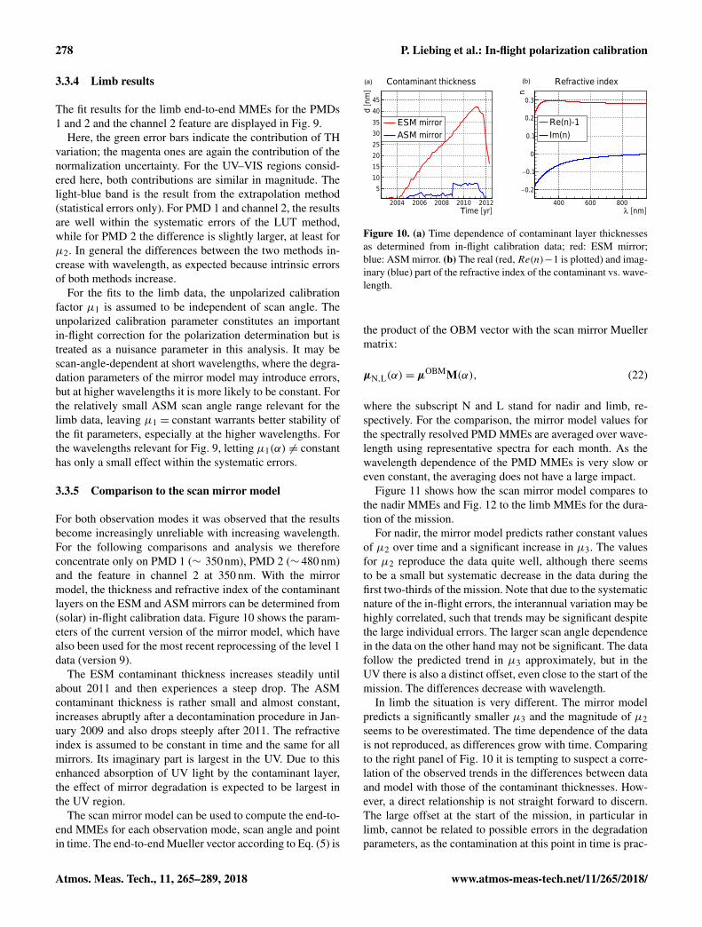
For both observation modes it was observed that the resultsbecome increasingly unreliable with increasing wavelength.For the following comparisons and analysis we thereforeconcentrate only on PMD 1 (∼ 350nm), PMD 2 (∼ 480 nm)and the feature in channel 2 at 350 nm. With the mirrormodel, the thickness and refractive index of the contaminantlayers on the ESM and ASM mirrors can be determined from(solar) in-flight calibration data. Figure 10 shows the param-eters of the current version of the mirror model, which havealso been used for the most recent reprocessing of the level 1data (version 9).
The ESM contaminant thickness increases steadily untilabout 2011 and then experiences a steep drop. The ASMcontaminant thickness is rather small and almost constant,increases abruptly after a decontamination procedure in Jan-uary 2009 and also drops steeply after 2011. The refractiveindex is assumed to be constant in time and the same for allmirrors. Its imaginary part is largest in the UV. Due to thisenhanced absorption of UV light by the contaminant layer,the effect of mirror degradation is expected to be largest inthe UV region.
The scan mirror model can be used to compute the end-to-end MMEs for each observation mode, scan angle and pointin time. The end-to-end Mueller vector according to Eq. (5) is
Figure 10. (a) Time dependence of contaminant layer thicknessesas determined from in-flight calibration data; red: ESM mirror;blue: ASM mirror. (b) The real (red, Re(n)−1 is plotted) and imag-inary (blue) part of the refractive index of the contaminant vs. wave-length.
the product of the OBM vector with the scan mirror Muellermatrix:
µN,L(α)= µOBMM(α), (22)
where the subscript N and L stand for nadir and limb, re-spectively. For the comparison, the mirror model values forthe spectrally resolved PMD MMEs are averaged over wave-length using representative spectra for each month. As thewavelength dependence of the PMD MMEs is very slow oreven constant, the averaging does not have a large impact.
Figure 11 shows how the scan mirror model compares tothe nadir MMEs and Fig. 12 to the limb MMEs for the dura-tion of the mission.
For nadir, the mirror model predicts rather constant valuesof µ2 over time and a significant increase in µ3. The valuesfor µ2 reproduce the data quite well, although there seemsto be a small but systematic decrease in the data during thefirst two-thirds of the mission. Note that due to the systematicnature of the in-flight errors, the interannual variation may behighly correlated, such that trends may be significant despitethe large individual errors. The larger scan angle dependencein the data on the other hand may not be significant. The datafollow the predicted trend in µ3 approximately, but in theUV there is also a distinct offset, even close to the start of themission. The differences decrease with wavelength.
In limb the situation is very different. The mirror modelpredicts a significantly smaller µ3 and the magnitude of µ2seems to be overestimated. The time dependence of the datais not reproduced, as differences grow with time. Comparingto the right panel of Fig. 10 it is tempting to suspect a corre-lation of the observed trends in the differences between dataand model with those of the contaminant thicknesses. How-ever, a direct relationship is not straight forward to discern.The large offset at the start of the mission, in particular inlimb, cannot be related to possible errors in the degradationparameters, as the contamination at this point in time is prac-
Atmos. Meas. Tech., 11, 265–289, 2018 www.atmos-meas-tech.net/11/265/2018/

P. Liebing et al.: In-flight polarization calibration 279
Figure 11. Time dependence of in-flight end-to-end Mueller matrix elements µ2 (a, c, e) and µ3 (b, d, f) for nadir for four selected ESMangles from measurements (data points) and the scan mirror model (lines). The error bars include statistical and total systematic errors. (a,b) Channel 2 feature; (c, d) PMD 1; (e, f) PMD 2. The color code signifies the ESM scan angle bin (−22, −11, +1, +13◦), increasing on arainbow color scale.
Figure 12. Time dependence of in-flight end-to-end Mueller matrix elements µ2 (a, c, e) and µ3 (b, d, f) for limb at TH≈ 28 km forfour selected ASM angles from measurements (data points) and the scan mirror model (lines). The error bars include statistical and totalsystematic errors. (a, b) Channel 2 feature; (c, d) PMD 1; (e, f) PMD 2. The color code signifies the ASM scan angle bin (−5,−1,+3,+7◦),increasing on a rainbow color scale.
www.atmos-meas-tech.net/11/265/2018/ Atmos. Meas. Tech., 11, 265–289, 2018

280 P. Liebing et al.: In-flight polarization calibration
tically nonexistent. The reason for this early discrepancy hasto lie in the OBM.
4 Interpretation of results
In this section, the results for the in-flight MMEs presentedabove will be interpreted with respect to a change in theOBM polarization sensitivities between the on-ground cal-ibration measurements and in-flight conditions. Already theon-ground calibration revealed an unexpectedly large sensi-tivity to 45◦ polarization end-to-end in nadir, mainly for thePMDs, but also for the science channels. The on-ground cali-bration campaign was performed for fixed OBM and detectortemperatures close to the in-flight temperature settings. Butsome dedicated measurements were done with varying OBMtemperatures, where polarization sensitivities were found tobe temperature dependent. The peculiar wavelength and tem-perature dependence thus pointed to temperature-inducedstress birefringence as the likely physical cause (Snel, 1999).The predisperser prism, being the only optical element in thelight path of both PMDs and science channels aside fromthe telescope, would serve as a viable originator of this phe-nomenon. Even though the prism mount was designed to bestress-free, it may be possible that through the mechanicalstress generated by the presence of temperature gradients in-side the instrument, birefringence can be generated. It is alsopossible that a small residual birefringence from the manu-facturing process of up to 5 nmcm−1 (Keller, 2001) can befurther enhanced due to stress. Under the microgravity con-ditions in-flight, stress may distribute differently, such thatthe experienced birefringence may change accordingly. Sev-eral analyses (Snel, 1999; Slijkhuis and Frerick, 1999) of theon-ground data arrived at different results for the parame-ters associated with the alleged phase shift, based on differ-ent presumptions, definitions and data. Here, we present ananalysis of the measured in-flight MMEs as well as the re-vised on-ground OBM MMEs performed consistently withinthe frame work of the scan mirror model in order to test thehypothesis of an unintended, stress-induced phase shift in-side the predisperser prism.
4.1 Retarder model
After the scanner module, the light beam enters the tele-scope where it undergoes reflections off the two parabolicaluminum mirrors under a small angle and within the sameplane. Under these conditions the polarization sensitivity ofthe telescope can be assumed to be negligible. A possible lossof reflectivity due to degradation would be common to bothPMDs and science channels and not be visible in the mea-sured polarization signal. After the telescope, the light entersthe predisperser prism, which consists of fused silica glass.It travels for about 1.5 cm before a part of the beam is inter-nally reflected at an angle close to the Brewster angle (∼ 34◦
for fused silica) and emerges nearly 100 % polarized to be di-rected towards the PMDs after yet another internal reflection,while the major, still partially polarized, part of the beam istransmitted towards the science channels (see Fig. 2 above).Thus, assuming the telescope does not affect the polarizedcomponents of the OBM vector, the scan mirror model canbe very simply extended by introducing the Mueller matrixfor a linear retarder to represent the part of the predisperserprism before the Brewster reflection that can be influencedby birefringence:
S = IMOBM11 µOBMR(δ,θ)M(α)(1,q,u,v)T , (23)
where R is the Mueller matrix of a linear retarder
R(δ,θ)=
1 0 0 00 c2
2 + s22 cosδ c2s2(1− cosδ) s2 sinδ
0 c2s2(1− cosδ) s22 + c
22 cosδ −c2 sinδ
0 −s2 sinδ c2 sinδ cosδ,
(24)
and
c2 ≡ cos2θ ands2 ≡ sin2θ. (25)
Depending on the retarder angle θ , the linear retarder simul-taneously rotates the plane of linear polarization and convertslinear into circularly polarized light (or vice versa), depend-ing on the retardance δ. At θ = 0 or 90◦, the crosstalk be-tween U and V is maximized, while at θ =±45◦ the con-version takes place entirely between Q and V . In terms ofa birefringent crystal or slab of material, θ describes the di-rection of the optic axis, with respect to which the incomingbeam is split into an ordinary (polarization direction perpen-dicular to the optic axis) and extraordinary ray (polarizationdirection perpendicular to that of the ordinary ray) and δ isthe retardance of the slower ray relative to the faster (typi-cally the ordinary) ray.
The retardance in a slab of thickness d is
δ =2πdλ(ne− no). (26)
The actual birefringence is the difference between the indicesof refraction for the extraordinary and ordinary ray, ne− no.For stress-induced birefringence, this can be related to
B ≡ ne− no = R(λ)(σ1− σ2)
=n(λ)3
2(q11− q12)(σ1− σ2), (27)
where σ1 and σ2 are the stresses along the polarization direc-tions of the ordinary and extraordinary rays, and q11 and q12are the components of the strain-optic tensor. The refractiveindex n is wavelength dependent. R is called the stress-opticconstant and also depends on wavelength (Sinha, 1978):
R(λ)= R(λ0)
[n(λ0)
n(λ)
][λ2
λ20
][λ2
0− λ21
λ2− λ21
][λ2− λ2
2
λ20− λ
22
], (28)
Atmos. Meas. Tech., 11, 265–289, 2018 www.atmos-meas-tech.net/11/265/2018/

P. Liebing et al.: In-flight polarization calibration 281
with λ1 = 121.5 nm, λ2 = 6900 nm and λ0 be-ing a normalization wavelength. For λ0 = 633nm,R = 35 ± 1nmcm−1 MPa−1 (Priestley, 2001). There-fore, it is possible to build a model that determines theretarder matrix for all wavelengths from a measurement ata single wavelength. Here, λ0 will be set to 300nm. Theretardance at any other wavelength can then be modeled as
δ(λ)= δ(λ0)λ0
λ
R(λ)
R(λ0). (29)
The retarder angle θ depends on the direction of the appliedstress. The type of stress discussed here may be distributednon-uniformly across the prism such that different parts ofthe beam experience different rotations. Since the relevantphase shift occurs before the Brewster reflection (PMDs) orbefore the exit from the prism (science channels) and there-fore also before wavelength dispersion, the averaged (overthe beam cross section) retarder angle can be assumed to bewavelength independent.
4.2 Fit of retarder parameters
Based on Eqs. (23) and (22), the vector of retarder parame-ters 2= (δ(λ0),θ) can be found in principle by minimizingthe difference between a modeled and measured end-to-endMueller vector:
χ2N,L =
(µMeas
N,L −X(2))T·6−1
·(µMeas
N,L −X(2)), (30)
with the instrument model
X(2)≡ µL,N (α,2)= µOBMR(δ,θ)M(α). (31)
The vector of measurement points µMeasN,L contains the mea-
sured µ2 and µ3, each for four selected scan angles in nadirand limb, respectively. The covariance matrix 6 is deter-mined from the total (statistical and systematic) error as de-scribed in Sect. 3.3.2.
4.2.1 Confidence regions
Instead of directly combining the nadir and limb data anddata for different detectors into one measurement vector, χ2
can be computed for each separately and the resulting dis-tribution as a function of (δ(λ0),θ) can be used to evaluatethe validity of the retarder model in terms of its intrinsic con-sistency. In an ideal case, the best fitting retarder parameterswould describe nadir and limb data and each detector equallywell. In a statistical sense this means that the regions with
1χ2= χ2(2)−χ2
Min <1χ2Max(p) (32)
for given confidence level p should overlap for individ-ual measurement modes and detectors. The confidence re-gion 2p includes all points 2 with probability P(χ2 >
χ2(2,ν))= 1−CDF(χ2,ν) > 1−p for a χ2 distribution
with ν degrees of freedom with the corresponding cumulativedistribution function (CDF). Here ν corresponds to the num-ber of considered fit parameters – in this case, ν = 2 (Presset al., 2007). Strictly, this interpretation is only valid if theerrors were purely statistical and Gaussian distributed. Thesystematics-dominated errors of the in-flight data are neither;nevertheless, this approach seems the only practically feasi-ble way to check consistency between independent measure-ments and combine them in order to maximize informationcontent and to estimate errors on the fit parameters and de-rived values. This approach is demonstrated in the following.
First, Fig. 13 shows the χ2 distribution for PMD 1, nadir(left panel) and limb (LUT method, right panel) in 2004. Theparameter range has been restricted to |δ| ≤ 45 and θ < 90◦
due to symmetries in the retarder matrix and because the χ2
for retardances outside the±45◦ limit increases even further.Inside the considered parameter space, χ2 varies by sev-
eral orders of magnitude. The plot also shows extended re-gions of minima located distinctly away from the zero point.
Next, the 99.99 % confidence regions for limb and nadirand different detectors (PMDs 1 and 2, channel 2) are shownin Fig. 14 for each considered year.
In 2003, the confidence regions for all detectors and mea-surement modes overlap in a common region of δ between 5and 10◦ and θ between 10 and 15◦. Except for PMD 1, thenadir regions also include a zero retardance, while all limbdata are located away from zero. For the following yearsit can be observed that the limb and nadir regions slowlydrift apart almost consistently for all detectors. While foreach measurement mode alone there is still an overlap, al-beit small, for all detectors, no common overlap exist evenfor individual detectors after about 2006. There are severalpossible reasons for this behavior, none of which can be rig-orously excluded: the retarder may be an inadequate modelto describe the OBM polarization degradation; the mirrordegradation parameters may not describe the mirror degrada-tion properly; or an unknown, time-dependent, systematic er-ror impairs the in-flight measurement and its error estimates.The effect of the mirror model degradation parameters is dis-cussed in Sect. 4.3.
Regarding OBM degradation other than the phase shift, itshould be considered that, at least for the PMDs, a degrada-tion of optical elements in the light path after the Brewster re-flection inside the prism will not depend on the Stokes vectorbefore the prism anymore; therefore, it can affect through-put, but not polarization. This argument holds as long as theprism acts as a near-perfect polarizer. It may be conceivablethat some effect, e.g., radiation damage, changes the refrac-tive index of the prism such that the efficiency of the internalBrewster reflection decreases. In such an event, the refrac-tive index change should be noticed elsewhere as well, forinstance in the form of a large wavelength shift of the mea-sured spectra. However, such an effect has not been observed.
www.atmos-meas-tech.net/11/265/2018/ Atmos. Meas. Tech., 11, 265–289, 2018

282 P. Liebing et al.: In-flight polarization calibration
Figure 13. χ2 distribution according to Eq. (30) for PMD 1, nadir (a) and limb (b) in 2004. The retardance parameter is on the x axis andthe retarder angle on the y axis; the color code depicts χ2 on a logarithmic (rainbow) color scale.
4.2.2 Determination of model parameters and errors
Especially in limb, it is important to have a time-dependentin-flight correction to the mirror model MMEs for all wave-lengths and PMDs and science channels alike. That is why,even though the observed drift of limb and nadir data doesnot raise too much confidence in the hypothesis of a time-dependent OBM phase shift, the retarder model is applied todetermine the most likely retarder parameters and their errorsas a function of time. This is done by the process of marginal-izing the respective other parameter, i.e., by integrating eachretarder parameter weighted with the likelihood derived fromthe CDF of the χ2 distribution (Verde, 2010). The likelihoodfor any combination of measurement modes and detectorscan be obtained from the product of the respective, normal-ized individual distributions:
LC(2Fit
)=
∏i
P i(2)∫P i(2)d2
. (33)
The mean values of a generic fit parameter or a derived pa-rameter 2 (such as the retarder-corrected in-flight MMEs)and their errors can be computed from this distribution asfollows:
〈2C〉 =
∫2CLC(2)d2, (34)
σ 2(2C)=
∫ (2−〈2C〉
)2LC(2)d2, (35)
for all considered combinations C.After deriving the retarder parameters in the initial anal-
ysis step, an iteration of the entire chain of fits has to beperformed. The reflectances and polarization signals are cor-rected for the polarization of the science channels with theMMEs computed with the retarder parameters from the ini-tial step, using Eq. (16) with the updated MMEs. The effectof this iteration on the value for the retardance is almost neg-ligible, but the retarder angle is shifted down by about 3◦.
4.2.3 Results
Figure 15 shows the results for the retarder parameters fordifferent observation modes and detector combinations afterthe iteration step.
It demonstrates how adding information from different de-tectors, e.g., PMD 1 and channel 2, or combining limb andnadir, subsequently changes retarder values and reduces er-rors. For instance, in nadir there is not much information onthe retarder angle because for small retardances χ2 (or like-wise the probability) does not depend on the retarder angle.In limb, larger retardances are favored and the retarder angleis therefore constrained better. The evident offset betweenchannel 2 and PMD 1 comes from the peculiar confidence re-gion of channel 2 which includes large values of θ > 45◦ andnegative retardances. Only the combination with the PMDsrestricts this region to θ < 30◦ and positive retardances. Theplot also shows how the combination of limb and nadir dataresults in a compromise which is dominated by the informa-tion contained in the limb data. For PMD 2, the sensitivity tothe phase shift is considerably smaller than for PMD 1 andchannel 2 due to its wavelength dependence, while the sen-sitivity to errors in the calibration is larger, as can be seenfor instance in the error bars of Fig. 11. Therefore, the fi-nal retarder values to be used for polarization determinationand correction will eventually be derived from a combina-tion of limb and nadir, PMD 1 and channel 2. The valuesshown in Fig. 15 were obtained with the LUT method for thePMDs in limb and the extrapolation method otherwise. Re-tarder parameters obtained by using the extrapolation methodin limb entirely differ by about 1 to maximum 2◦ for the finalresult. Parameters change within a similar margin when theoff-diagonal elements in the systematic covariance matrix areset to zero.
The end-to-end MMEs calculated from the retarder modelwith the fitted parameters are shown in Figs. 16 and 17 to-gether with the MMEs calculated from the original mirrormodel and the in-flight data. The errors on the end-to-end
Atmos. Meas. Tech., 11, 265–289, 2018 www.atmos-meas-tech.net/11/265/2018/

P. Liebing et al.: In-flight polarization calibration 283
Figure 14. The 99.99 % confidence region contours for limb and nadir, PMDs 1 and 2, and channel 2 for each year starting from 2003 (topleft) to 2011 (bottom right).
MMEs (Eq. 34) are typically less than a few 10−3 and there-fore much smaller than the error on the data, which is whythey are not shown on the plot.
The retarder model seems to fix the largest differences innadir and mostly also in limb. An issue remains with the timedependence in limb, especially towards the later part of themission. The main effect of the retarder model applied to
the data will be an improvement of the polarization deter-mination, reducing systematic errors in the limb UV down toabout 10 % and therefore by a factor of about 2. The polar-ization correction in the UV in channel 1 and for channel 2around 350 nm will also considerably improve. However, thecalibration for the unpolarized response will be nearly unaf-fected.
www.atmos-meas-tech.net/11/265/2018/ Atmos. Meas. Tech., 11, 265–289, 2018
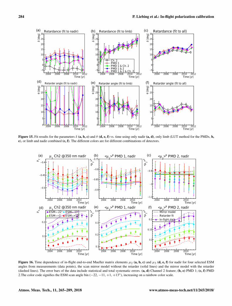
284 P. Liebing et al.: In-flight polarization calibration
Figure 15. Fit results for the parameters δ (a, b, c) and θ (d, e, f) vs. time using only nadir (a, d), only limb (LUT method for the PMDs, b,e), or limb and nadir combined (c, f). The different colors are for different combinations of detectors.
Figure 16. Time dependence of in-flight end-to-end Mueller matrix elements µ2 (a, b, c) and µ3 (d, e, f) for nadir for four selected ESMangles from measurements (data points), the scan mirror model without the retarder (solid lines) and the mirror model with the retarder(dashed lines). The error bars of the data include statistical and total systematic errors. (a, d) Channel 2 feature; (b, e) PMD 1; (c, f) PMD2.The color code signifies the ESM scan angle bin (−22, −11, +1, +13◦), increasing on a rainbow color scale.
Atmos. Meas. Tech., 11, 265–289, 2018 www.atmos-meas-tech.net/11/265/2018/

P. Liebing et al.: In-flight polarization calibration 285
Figure 17. Time dependence of in-flight end-to-end Mueller matrix elements µ2 (a, b, c) and µ3 (d, e, f) for limb at TH≈ 28 km for fourselected ASM angles from measurements (data points), the scan mirror model without the retarder (solid lines) and the mirror model withthe retarder (dashed lines). The error bars include statistical and total systematic errors. (a, d) Channel 2 feature; (b, e) PMD 1; (c, f) PMD2. The color code signifies the ASM scan angle bin (−5, −1, +3, +7◦), increasing on a rainbow color scale.
4.3 Dependence of retarder parameters on the scanmirror model
The fit procedure described in Sect. 4.2 can be applied in ananalogous way to fit parameters of the mirror degradation,i.e., thicknesses on ESM and ASM mirrors and the refrac-tive index at 350 (using PMD 1 and channel 2) and 480 nm(using PMD 2). The measurement vectors used are the sameas for the retarder fit. The combination of different detectorsand observation modes is more complex in such a fit becauseof the relationship of the fit parameters to certain subsets ofdata. The fit aims at constraining these six independent pa-rameters from selected detector and observation mode com-binations which maximize the information content. The in-vestigated range was from 0 to 100 nm in contaminant thick-nesses, from 1 to 1.5 for the real part and from −0.5 to 0 inthe imaginary part of the refractive index.
Together with the unpolarized response constrained to liewithin limits consistent with the solar calibration data, the al-lowed parameter range can be considerably reduced. Fit pa-rameters, for instance thickness and refractive index, tend tobe highly anticorrelated. This can be explained by the equa-tions describing the effect of a thin layer such as the contam-inant on the mirror substrate, where the relevant term for thereflection coefficient enters as a product of layer thicknessand refractive index (Krijger et al., 2014). This high correla-tion inhibits the unambiguous determination of all parame-
ters, but a few qualitative statements can be made based onthis investigation.
First, within the scanned parameter range, it is not possibleto find a physically reasonable set of parameters that coulddescribe the measured in-flight MMEs without an additionalphase shift introduced by the retarder. This finding provesthat there is indeed an on-ground to in-flight change insidethe OBM. Second, it is possible to find physically reasonablesets of parameters that fit the data when fixing the retarder pa-rameters to those obtained for 2003. That means that a singleon-ground to in-flight change in the OBM would suffice todescribe the measurements at all times in combination withmirror model parameters that tend to be different from theones derived from unpolarized calibration data (see Fig. 10).In particular, the range of possible combinations of thicknessand refractive index is inconsistent with those values. In fact,applying a time-dependent refractive index with a constantphase shift consistently leads to better agreement betweenthe model and data than a time-dependent phase shift with aconstant refractive index.
At the very least this means that the thicker the contami-nation layer is, the more the retarder parameters depend onthe mirror model parameters. Furthermore, the findings sug-gest that the inclusion of polarization data into the fits of themirror degradation parameters may improve or even resolvethe degeneracy between different fit parameters.
www.atmos-meas-tech.net/11/265/2018/ Atmos. Meas. Tech., 11, 265–289, 2018
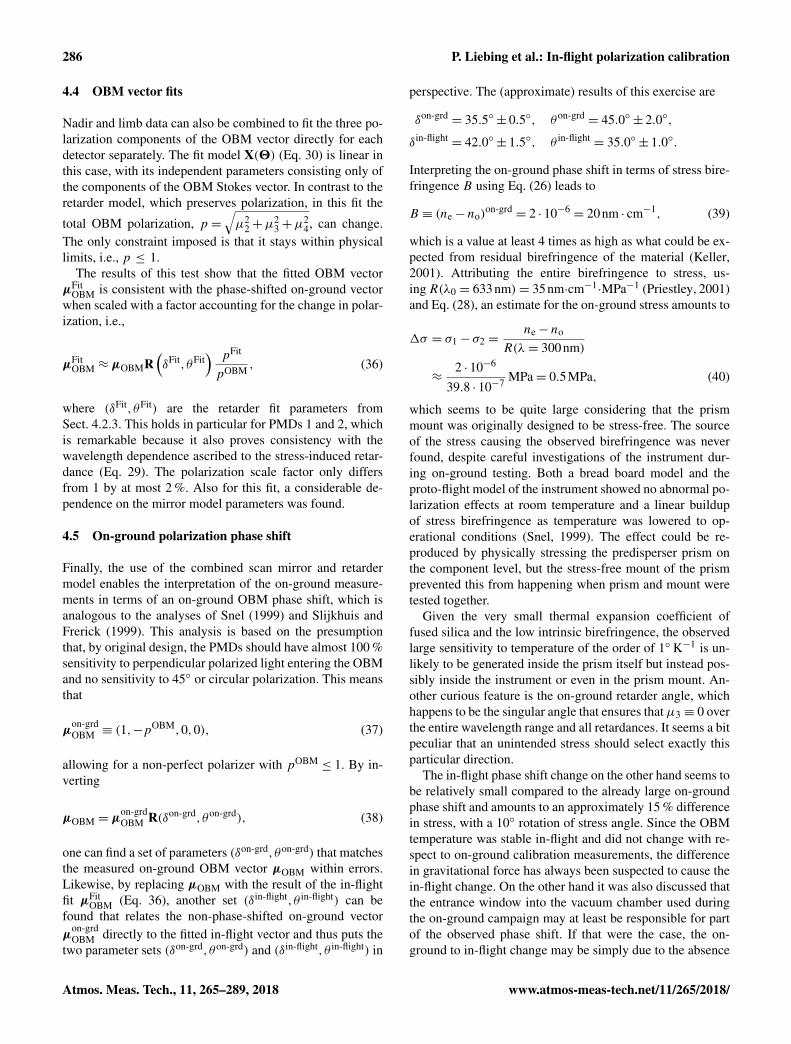
286 P. Liebing et al.: In-flight polarization calibration
4.4 OBM vector fits
Nadir and limb data can also be combined to fit the three po-larization components of the OBM vector directly for eachdetector separately. The fit model X(2) (Eq. 30) is linear inthis case, with its independent parameters consisting only ofthe components of the OBM Stokes vector. In contrast to theretarder model, which preserves polarization, in this fit the
total OBM polarization, p =õ2
2+µ23+µ
24, can change.
The only constraint imposed is that it stays within physicallimits, i.e., p ≤ 1.
The results of this test show that the fitted OBM vectorµFit
OBM is consistent with the phase-shifted on-ground vectorwhen scaled with a factor accounting for the change in polar-ization, i.e.,
µFitOBM ≈ µOBMR
(δFit,θFit
) pFit
pOBM , (36)
where (δFit,θFit) are the retarder fit parameters fromSect. 4.2.3. This holds in particular for PMDs 1 and 2, whichis remarkable because it also proves consistency with thewavelength dependence ascribed to the stress-induced retar-dance (Eq. 29). The polarization scale factor only differsfrom 1 by at most 2 %. Also for this fit, a considerable de-pendence on the mirror model parameters was found.
4.5 On-ground polarization phase shift
Finally, the use of the combined scan mirror and retardermodel enables the interpretation of the on-ground measure-ments in terms of an on-ground OBM phase shift, which isanalogous to the analyses of Snel (1999) and Slijkhuis andFrerick (1999). This analysis is based on the presumptionthat, by original design, the PMDs should have almost 100 %sensitivity to perpendicular polarized light entering the OBMand no sensitivity to 45◦ or circular polarization. This meansthat
µon-grdOBM ≡ (1,−p
OBM,0,0), (37)
allowing for a non-perfect polarizer with pOBM≤ 1. By in-
verting
µOBM = µon-grdOBM R(δon-grd,θon-grd), (38)
one can find a set of parameters (δon-grd,θon-grd) that matchesthe measured on-ground OBM vector µOBM within errors.Likewise, by replacing µOBM with the result of the in-flightfit µFit
OBM (Eq. 36), another set (δin-flight,θ in-flight) can befound that relates the non-phase-shifted on-ground vectorµ
on-grdOBM directly to the fitted in-flight vector and thus puts the
two parameter sets (δon-grd,θon-grd) and (δin-flight,θ in-flight) in
perspective. The (approximate) results of this exercise are
δon-grd= 35.5◦± 0.5◦, θon-grd
= 45.0◦± 2.0◦,
δin-flight= 42.0◦± 1.5◦, θ in-flight
= 35.0◦± 1.0◦.
Interpreting the on-ground phase shift in terms of stress bire-fringence B using Eq. (26) leads to
B ≡ (ne− no)on-grd
= 2 · 10−6= 20nm · cm−1, (39)
which is a value at least 4 times as high as what could be ex-pected from residual birefringence of the material (Keller,2001). Attributing the entire birefringence to stress, us-ingR(λ0 = 633nm)= 35nm·cm−1
·MPa−1 (Priestley, 2001)and Eq. (28), an estimate for the on-ground stress amounts to
1σ = σ1− σ2 =ne− no
R(λ= 300nm)
≈2 · 10−6
39.8 · 10−7 MPa= 0.5MPa, (40)
which seems to be quite large considering that the prismmount was originally designed to be stress-free. The sourceof the stress causing the observed birefringence was neverfound, despite careful investigations of the instrument dur-ing on-ground testing. Both a bread board model and theproto-flight model of the instrument showed no abnormal po-larization effects at room temperature and a linear buildupof stress birefringence as temperature was lowered to op-erational conditions (Snel, 1999). The effect could be re-produced by physically stressing the predisperser prism onthe component level, but the stress-free mount of the prismprevented this from happening when prism and mount weretested together.
Given the very small thermal expansion coefficient offused silica and the low intrinsic birefringence, the observedlarge sensitivity to temperature of the order of 1◦ K−1 is un-likely to be generated inside the prism itself but instead pos-sibly inside the instrument or even in the prism mount. An-other curious feature is the on-ground retarder angle, whichhappens to be the singular angle that ensures thatµ3 ≡ 0 overthe entire wavelength range and all retardances. It seems a bitpeculiar that an unintended stress should select exactly thisparticular direction.
The in-flight phase shift change on the other hand seems tobe relatively small compared to the already large on-groundphase shift and amounts to an approximately 15 % differencein stress, with a 10◦ rotation of stress angle. Since the OBMtemperature was stable in-flight and did not change with re-spect to on-ground calibration measurements, the differencein gravitational force has always been suspected to cause thein-flight change. On the other hand it was also discussed thatthe entrance window into the vacuum chamber used duringthe on-ground campaign may at least be responsible for partof the observed phase shift. If that were the case, the on-ground to in-flight change may be simply due to the absence
Atmos. Meas. Tech., 11, 265–289, 2018 www.atmos-meas-tech.net/11/265/2018/

P. Liebing et al.: In-flight polarization calibration 287
of this so-called “OPTEC window” in flight. With the cur-rently available data, it is not possible to clearly identify thereason for the observed behavior on the ground and in flight.Further analysis of all available calibration data may be nec-essary.
5 Conclusions
A novel statistical approach for the in-flight polarization cal-ibration of the SCIAMACHY PMDs and a part of its sciencechannels is presented. It exploits the relationship betweenpolarization and measured reflectance. This approach can inprinciple be further refined and adapted for the polarizationcalibration of other instruments which measure polarization,such as GOME, GOME-2 or even POLDER/PARASOL.The overarching requirements for the polarization sensitiv-ity measurement are a sufficiently accurate model or dataapplicable to the particular measurement conditions or suffi-cient statistics and leverage to extrapolate to a limiting modelto determine polarization signals. The resulting polarizationsignals should cover a significant portion of the (q,u) planeto provide enough leverage for the determination of polariza-tion sensitivities.
The general applicability to other instruments has not beendiscussed in much detail here because it depends on the spe-cific instrument, its measurement modes and available data.Limiting models can be in principle improved by includinginformation on known wind speeds or surface reflectance.An extension of well-established calibration methods em-ploying natural targets (see Frouin, 2013, for an overview)with the extrapolation method to include polarization mayalso be worth considering. For SCIAMACHY, however, us-ing a few selected oceanic sites resulted in too-small lever-age in (q,u) to retrieve meaningful information; for otherinstruments such as PARASOL or MODIS with many ob-servations of the same scene from different angles, this maynot pose a problem. For MODIS, for instance, cross calibra-tion with SeaWiFS data and modeled polarization values hasbeen successfully applied (Meister et al., 2009). The modeledrelationship between reflectance and polarization may be re-placed by suitable data, such as accurately calibrated datafrom the POLDER or PARASOL instruments. Co-located re-flectance measurements may provide a reference reflectanceto determine polarization signals when dedicated polariza-tion measurements are not available. For instance, the com-bination of MERIS reflectance data co-located with SCIA-MACHY measurements, together with a statistical distribu-tion of (q,u) vs. reflectance derived from PARASOL datamatched with SCIAMACHY viewing geometries, resulted inan independent measurement of science channel polarizationsignals at MERIS wavelengths, e.g., 510, 665 and 885 nm.The derived polarization sensitivities for nadir were roughlyconsistent with expectation (Liebing et al., 2014). The inves-tigated time span was only 1 month, August 2007, such that
any further interpretation of the results was inhibited by too-large uncertainties.
The results presented here are based on the polarization–reflectance relationship inferred directly from RTM simula-tions or extrapolated to a limiting case. For wavelengths be-low ∼ 500 nm they prove to be stable enough for further in-vestigation of the instrument degradation. First, it was foundthat the instrument model used to calibrate the scan-angle-dependent degradation of SCIAMACHY due to contamina-tion of its scan mirrors neither reproduces the in-flight polar-ization sensitivities in these channels at the beginning of themission nor their time dependence. The effect is largest forthe limb data. Second, the observed discrepancies betweenthe model and data in the early part of the mission couldbe clearly traced back to an on-ground to in-flight change inthe polarization sensitivity inside the optical bench of the in-strument. The values are consistent with an extended instru-ment model that includes both the mirror degradation andstress-induced birefringence inside the predisperser prism.The model was used to fit the parameters of a linear retarderthat generates a polarization phase shift.
Several tests were performed to investigate the reason forthe observed phase shift, both on the ground and in flight,as well as its time dependence. A retrospect analysis of theon-ground calibration data shows that an unexplained, largephase shift was already present at that time and that the dif-ference between the on-ground and in-flight phase shifts iscomparatively small. The time dependence may indeed bean artifact of the scan mirror model, resulting from the im-posed assumptions on the properties of the mirror contami-nant. Since the polarization data show a sizeable sensitivity tothese properties, the inclusion of these data in addition to thesolar measurements in the calibration approach of the scanmirror model may actually help to disentangle some of theambiguities between different degradation parameters.
Even though the search for the origin of the phase shift re-mained inconclusive, the results of this investigation consid-erably improve the polarization calibration of the measuredSCIAMACHY radiances, in particular in limb. As an addedbenefit, the new calibration, together with an improved al-gorithm applied in version 9 of the operational level 0 to 1processor, enables the determination of the atmospheric po-larization, i.e., Stokes q for all PMD wavelengths and u at850 nm, with a relative accuracy on the order of 10 %. Al-though this is far from the accuracies achieved by dedicatedinstruments such as POLDER, the new SCIAMACHY po-larization data may provide valuable additional information– on a statistical basis – on, for example, cloud or aerosolproperties for suitable observing geometries.
Data availability. This analysis was performed using opera-tional level 1B SCIAMACHY data (version 8), accessible viahttps://earth.esa.int/web/guest/-/sciamachy-localized-atmospheric-spectra-in-the-uvvisnear-ir.
www.atmos-meas-tech.net/11/265/2018/ Atmos. Meas. Tech., 11, 265–289, 2018
288 P. Liebing et al.: In-flight polarization calibration
Competing interests. The authors declare that they have no conflictof interest.
Acknowledgements. SCIAMACHY is a national contribution tothe ESA Envisat project, funded by Germany, the Netherlands andBelgium. SCIAMACHY data have been provided by ESA. Thiswork has been funded by the German Aerospace Center (DLR), theSCIAMACHY Quality Working Group project (ESA) and by theUniversity of Bremen.
The article processing charges for this open-accesspublication were covered by the University of Bremen.
Edited by: Udo FriessReviewed by: Ruediger Lang and one anonymous referee
References
Bovensmann, H., Burrows, J. P., Buchwitz, M., Frerick, J., Noël,S., Rozanov, V. V., Chance, K. V., and Goede, A. H. P.: SCIA-MACHY – Mission Objectives and Measurement Modes, J. At-mos. Sci., 56, 127–150, 1999.
Cox, C. and Munk, W.: Measurement of the Roughness of the SeaSurface from Photographs of the Sun’s Glitter, J. Opt. Soc. Am.,44, 838–850, https://doi.org/10.1364/JOSA.44.000838, 1954.
Emde, C. and Mayer, B.: Simulation of solar radiation during a totaleclipse: a challenge for radiative transfer, Atmos. Chem. Phys.,7, 2259–2270, https://doi.org/10.5194/acp-7-2259-2007, 2007.
Frouin, R. (Ed.): In-flight Calibration of Satellite Ocean-ColourSensors, Vol. No. 14 of Reports of the International OceanColour Coordinating Group, IOCCG, Dartmouth, Canada, avail-able at: http://www.ioccg.org/reports/IOCCG_Report_14_2013.pdf (last access: 7 January 2018), 2013.
Gottwald, M. and Bovensmann, H. (Eds.): SCIAMACHY – Explor-ing the Changing Earth’s Atmosphere, Springer, Dordrecht Hei-delberg London New York, https://doi.org/10.1007/978-90-481-9896-2, 2011.
Keller, C. U.: Instrumentation for Astrophysical Spectropo-larimetry, in: Astrophysical Spectropolarimetry, editedby: Trujillo-Bueno, J., Moreno-Insertis, F., and Sanchez,F., Cambridge University Press, Cambridge, 303–354,https://doi.org/10.1017/CBO9780511564802.012, 2001.
Kokhanovsky, A. A., Budak, V. P., Cornet, C., Duan, M.,Emde, C., Katsev, I. L., Klyukov, D. A., Korkin, S. V.,C-Labonnote, L., Mayer, B., Min, Q., Nakajima, T., Ota,Y., Prikhach, A. S., Rozanov, V. V., Yokota, T., andZege, E. P.: Benchmark results in vector atmospheric ra-diative transfer, J. Quant. Spectrosc. Ra., 111, 1931–1946,https://doi.org/10.1016/j.jqsrt.2010.03.005, 2010.
Krijger, J. M.: SCIAMACHY On-Ground Polarisation Recalibra-tion, SRON-SQWG3_TN-2017-001, SRON, 2017.
Krijger, J. M., Tanzi, C. P., Aben, I., and Paul, F.: Val-idation of GOME polarization measurements by methodof limiting atmospheres, J. Geophys. Res., 110, D07305,https://doi.org/10.1029/2004JD005184, 2004.
Krijger, J. M., Snel, R., van Harten, G., Rietjens, J. H. H., and Aben,I.: Mirror contamination in space I: mirror modelling, Atmos.
Meas. Tech., 7, 3387–3398, https://doi.org/10.5194/amt-7-3387-2014, 2014.
Liebing, P., Bramstedt, K., Noël, S., Rozanov, V., Bovensmann,H., and Burrows, J. P.: Polarization data from SCIAMACHYlimb backscatter observations compared to vector radiative trans-fer model simulations, Atmos. Meas. Tech., 6, 1503–1520,https://doi.org/10.5194/amt-6-1503-2013, 2013.
Liebing, P., Snel, R., Bramstedt, K., and Krijger, M.: An Assess-ment of the In-flight Polarization Response of SCIAMACHY,AGU Fall Meeting Abstracts, available at: http://www.iup.uni-bremen.de/sciamachy/polarisation/AGU/SciaPol_pix.pdf(last access: 7 January 2018), 2014.
Maystre, D.: Theory of Wood’s Anomalies, in: Plasmonics: FromBasics to Advanced Topics (Springer Series in Optical Sciences),Springer, 2012.
McLinden, C. A., Haley, C. S., Lloyd, N. D., Hendrick, F.,Rozanov, A., Sinnhuber, B.-M., Goutail, F., Degenstein, D. A.,Llewellyn, E. J., Sioris, C. E., Roozendael, M. V., Pom-mereau, J. P., Lotz, W., and Burrows, J. P.: Odin/OSIRIS ob-servations of stratospheric BrO: Retrieval methodology, cli-matology, and inferred Bry , J. Geophys. Res., 115, D15308,https://doi.org/10.1029/2009JD012488, 2010.
Meister, G., Franz, B. A., Kwiatkowska, E. J., Eplee, R. E., and Mc-Clain, C. R.: Detector dependency of MODIS polarization sen-sitivity derived from on-orbit characterization, Proc. SPIE, 7452,7452, https://doi.org/10.1117/12.825385, 2009.
Press, W. H., Teukolsky, S. A., Vetterling, W. T., and Flannery, B. P.:Numerical Recipes 3rd Edn.: The Art of Scientific Computing,Cambridge University Press, New York, NY, USA, 3 Edn., 2007.
Priestley, R.: Birefringence dispersion in fused silicafor DUV lithography, Proc. SPIE, 4346, 1300–1305,https://doi.org/10.1117/12.435666, 2001.
Rozanov, V., Rozanov, A., Kokhanovsky, A., and Burrows, J.: Ra-diative transfer through terrestrial atmosphere and ocean: Soft-ware package {SCIATRAN}, J. Quant. Spectrosc. Ra., 133, 13–71, https://doi.org/10.1016/j.jqsrt.2013.07.004, 2014.
Rozanov, V. V. and Rozanov, A. V.: Software Package SCIATRAN(Radiative Transfer Model and Retrieval Algorithm), IUP, avail-able at: http://www.iup.uni-bremen.de/sciatran/free_downloads/users_guide_sciatran.pdf (last access: 7 January 2018), 2016.
Sinha, N. K.: Normalised dispersion of birefringence of quartz andstress optical coefficient of fused silica and plate glass, Phys.Chem. Glasses, 19, 69–77, 1978.
Sinnhuber, B.-M., Sheode, N., Sinnhuber, M., Chipperfield, M. P.,and Feng, W.: The contribution of anthropogenic bromine emis-sions to past stratospheric ozone trends: a modelling study, At-mos. Chem. Phys., 9, 2863–2871, https://doi.org/10.5194/acp-9-2863-2009, 2009.
Slijkhuis, S. and Frerick, J.: SCIAMACHY Polarisation Sensitivity,in: ERS-ENVISAT Symposium “Looking down to Earth in theNew Millennium”, 461, p. 1, 1999.
Snel, R.: SCIAMACHY on-ground performance: polarisation phaseshift, in: Proceedings of ESAMS’99 – European Symposium onAtmospheric Measurements from Space, ESTEC, Nordwijk, Thenetherlands, 18–22 January 1999 (WPP 161, Vol. 2), ESA, Nord-wijk, Netherlands, 725–729, 1999.
Atmos. Meas. Tech., 11, 265–289, 2018 www.atmos-meas-tech.net/11/265/2018/

P. Liebing et al.: In-flight polarization calibration 289
Tilstra, L. G. and Stammes, P.: Earth reflectance and polarizationintercomparison between SCIAMACHY onboard Envisat andPOLDER onboard ADEOS-2, J. Geophys. Res., 112, D11304,https://doi.org/10.1029/2006JD007713, 2007.
Tilstra, L. G. and Stammes, P.: SCIAMACHY Level-1 V7.03: EarthReflectance and Polarisation, KNMI-RP-2010-01, KNMI, 2010.
Verde, L.: Statistical Methods in Cosmology, in: Lecture Notes inPhysics, Berlin Springer Verlag, edited by: Wolschin, G., Vol.800 of Lecture Notes in Physics, Berlin Springer Verlag, 147–177, https://doi.org/10.1007/978-3-642-10598-2_4, 2010.
von Savigny, C., Ulasi, E. P., Eichmann, K.-U., Bovensmann, H.,and Burrows, J. P.: Detection and mapping of polar stratosphericclouds using limb scattering observations, Atmos. Chem. Phys.,5, 3071–3079, https://doi.org/10.5194/acp-5-3071-2005, 2005.
www.atmos-meas-tech.net/11/265/2018/ Atmos. Meas. Tech., 11, 265–289, 2018