FAA-ADS. 46

IN EVALUATIEI OF THE HEIG0:T VELOCITYlitDIAGUý, OF A LIGBMIG:1T,

LOV RO-f IETIA,L0 10T IN~l tEnil,"SINGLE ENGI IE IIELICOPTEn

TECHNICAL REPORTCLEARINGHOU3E

FOA FEDERAL SCIENTIFiC' ANDTECHNICAL iNF',;0MATION

Kirdcop----yi Miecrofiche i

a~~~l 4~ E~J±A 7

JULY 1965

byWILLIAM J. HANLEY

GILBERT DeVORE

Best Available Copy

FEDERAL AVIATION AGENCYAIRCRAFT DEVELOPMENT SERVICE

a oo,4O70a 0 G

AN EVALUATION OF THE HEIGHT VELOCITY DIAGRAM OF ALIGHTWEIGHT, LOW ROTOR INERTIA, SINGLE ENGINE HELICOPTER

0

TECHNICAL REPORTADS - 46

by

WILLIAM J. HANLEYGILBERT DE VORE

SYSTEMS RESEARCH AND DEVELOPMENT SERVICE

July 1965

This report was prepared by the SRDSunder Project No. 540-006-OIX for the

Aircraft Development Service

Z.,, -

TABLE OF CONTENTS

Page

LIST OF ILLUSTRATIONS. ...... . .o..... .

LiST OF TABLES . . . . . . . . it

INTRODUCIION . . . . e . . . e . * . . . o . * . . . . I . . * 1S Background . . . . . . . . . . . . . . .. . . . . . . . 1 i

Purpose . . . . . . . . . . . . . . . . . . . . . .. 0 !

Background o. . . .o .. . . . . . I

DISCUSSION .. .. . .... . ... . .... o 2

Test Aircraft . . . . . . . . . . . . . . . . .. . . . 2

Test Instrunentation . . . . . .. . . .. a . 2

lest Operations and Procedures . . . . .. .. .. .. 2

Flight Test Sites . .a . . . . . . . .. .. . .. 2

Test Methodology . . . . . 0 a . . . . . . . 2

Test Criteria . . . . . . . . . . . . . . . . . 3

ANALYSIS AND RESULTS . .. .. .. .. ...... .... 5

Discussion of Tests . . . . . . . . . . . . . . . . . . . 5

Height-Velocity Diagrams ................ 6

Discussion of One-Second Delay . . . . . . . . 8

Effects of Weight and Altitude . . . . .. . . . ..... 8

Equations .... . . ........ o . . . . .. . .. . 9

CONCLUSIONS . . . . o . o . . . o o o o * o 11

REFERENCES AND BIBLIOGRAPHY . . . . . .. .. .. ....... 12

TABLE OF CONTENTS CONTINUED

APPENDIX 1

Test Aircraft Specifications and Instrumontation Details

(9 pages)

APPENDIX 2

Pilot's Commnents (8 pages)

APPENDIX 3

Summary of Height-Velocity Diagram Flight Test Data (3 pages)

LIST OF ILLUSTRATIONS

Figure ?ase

I Typical Height-Velocity Aagram .......... 15

2 Test Aircraft ........ . . . . . . . . . 16

3 Typical Test SiLe Layout ..... ....... . . . . . 17

4 Height-Velocity Diagrams - Basic Data. Helicopter GrossWeight, 1450 pounds. Three Density Altitudes Shown . . . 18

5 Height-Velocity Diagrams - Basic Data. Helicopter CrossWeight, 1600 pounds. Two Density Altitudes Shown .... 19

6 Height-Velocity Diagram Variation with Density Altitudeand Cross Weight. No Delay and Delay Conditions Shown . . 20

7 Height-Velocity )iagram Variation with Density Altitude.Cross Weights of 1450 and 1600 pounds. Delay and NoDelay Conditions Shown .... ........... . .. . . . . . 21

8 Height Velocity Diagram Variation with Gross Weight. Two

Density Altitudes Shown for Delay and No Delay Conditions . 22

9 Comparison of Time History Data foi High Hover Points . . 23

10 Comparison of Time History Data for Critical Speed Area(Vcr, hcr) .................. ................ .. 24

11 Comparison of Time History Data for Low Hover Points . . . 25

12 Critical Velocity (Vcr) versus Aircraft Gross Weight forthe Range of Test Density Altitudes ................ 26

13 Critical Velocity (Vcr) versus Test Altitude For the Rangeof Test Weights ......... ................ . . . . . . . 26

14 Low Hover Height (hnmax) versus Aircraft Gross Weight forthe Range of Test Density Altitudes ..... ............ ... 27

15 Low Hover Height (hmax) versus Test Altitude for the Rangeof Test Weights ............... . ............ 0 27

16 High Ho',er Height (hmin) versus Square of CriticalVelucity (V 2cr) . . . . . . . . . .. . . . . . . . . . . 28

ILIST OF TABLES

Table Page

I Sumnary of High Hover (hmin) and Near High Hover . . . .. 13

II Sumary of Typical Data Area oF Critical Speed (Vcr) andCritcal Heigt (hcr) 14

r ca •i i

SUMfARY

A series of flight tests was conducted at three selected altitudes(sea level, 5000 feet, 7000 feet) to determine the effects of altitudeand weight on the height-velocity (H-V) diagram of a small, lightweight,low rotor inertia, medium disk loading, single rotor, single enginehelicopter. Two gross weights of the helicopter were used. Quantita-tive and qualitative test data were collected to determine how the H-Vdiagram varies with density altitude and aircraft gross weight. Aninvestigation was made into the effects on the diagram of a delayedcollective pitch application response.

Results disclosed a family of curves showing that increases indensity altitude and/or gross weight enlarged the H-V diagram requiredfor a sa.. r ff landing, Ana!ysis of Oie results revealed thatthe key points (Vcr, hmlin, and hnmx), which partially define the curves,could be determined by the solution of a set of linear equations. Theseresults were identical to those reported in FAA Technical Report ADS-lexcept for the constants of the linear equations and the location of thecritical height (hcr). The critical height indicated a slight increaseas weight, altitude and collective pitch reduction time delay wereincreased. An average value for hcr can be sQlected without upsettingthe family of curves.

iii

I - I . .

SYMBOLS

Vr critical velocity. The speed above which an autoro.ativelanding can be made from any height after power failurein the low speed regime, mph, CAS.

hcr a the height above the ground at which Vcr occurs, ft.

hwin the high hover height - the height auove the ground fromabove which a safe autorotative landing can be made afterpower failure at zero airspeed, ft.

hma the low hover height - the height ibove the ground frombelow which a safe power off landing can be made after powerfailure at zero airspeed, ft.

HD - density altitude at the point of landing, ft.

h a height of the helicopter above the ground, ft.

W a helicopter weight, lb.

CAS - calibrated airspeed - indicated airspeed corrected forinstrument and position error, mph.

iv

INTRODUCTION

The purpose of this project was to determine by flight tests theeffects of altitude and weight on the height-velocity (H-V) diagrams ofa small single-rotor helicopter which has an inherently low rotorinertia and medium disk loading.

Background

This flight test project is a continuation of a program initiatedby the Aircraft Development Service. Federal Aviation Agency, to acquire:ufficient actual flight test data on certai, basic helicopter flightparameters associated with the determination of the H-V diagram. Thtultimate objective of this program is to obtain a practical technicalapproach for the determination of the effects of altitude on thehelicopter H-V diagram.

The H-V diagram is a chart which defines an envelope of flight withrespect to airspeed and height above the ground where, in the event ofpower failure, a safe power off landing could not be effected. A typicalH-V diagram as referred to in this report is shown in Fig. 1 and wasestablished from eteady-state level flight conditions.

The flight test project of this program as reported in Reference 1was the first project undertaken to obtain flight test data on the power-off landing performance of a helicopter as the density altitude and grossweight are varied. The results of this project were succpssful in thatthe data were obtained and subsequent analysic disclosed that the H-Vdiagrams of the helicopter tested resolved Into a family of curves as afunction of weight and altitude. It was also concluded that this familyof curves could be defined by empirical equations involving key pointssuch as Vcr, hmin and hmax as shown in Fig. I in which hcr appears to

occur at a constant height abovc the grovnd. The sub-program scheduledadditional testing utilizing two single rotor helicopters of widely differentcharacteristics than the test vehicle used in Reference I in orler to obtainan adequate data spread on helicopters of different characteristics.

The helicopter utilized for the tests reported herein generallyrepresents one extreme in the spectrum of current single-enginehelicopters with respect to gross weight, disk loading and rotor inertiaconsiderations. The ether extreme of the spectrum - a large, high gross-weight helicopter of high totor inertia may be the target for futureendeavor with a follow-on comprehensive study correlating the facts ofall testing in this specific area of cons~deration.

1

DISCUSSION

Test Aircraft

The test vehicle wis a small, lightweight, sinole rotor, single-engine helicopter as shown in Fig. 2. This aircraft was selected forthis H-V test program because of its relatively low rotor inertia andmedium disk loading. Pertinent specifications of this aircraft arepresented in Appendix 1.

Test Instrumentation

Airborne and ground instrumentation was utilized to recordhelicopter performance and meteorological data. Details of the quantita-tive information measured and the equipment utilized are presented inAppendix 1.

Test Operations and Procedures

1. Flight Test Sites

The flight test project was conducted at three centrally locatedtest sites in the State of California during the period from October 6,1965, through December 8, 1965. These test sites, selected for theirelevation and test environment, were as follows:

Fresno Municipal Airport Elevation 332 ft. MSLBishop Municipal Elevation 4118 ft. MSLLong Valley Landing Strip Elevation 7120 ft. MSL

A schematic view of the test site layout showing the relativelocations of the test course, space positioning equipment, centralmarkers and meteorological equipment used for the flight tests is shownin Fig. 3.

2. Test Methodology

A professional engineering test pilot well skilled in themechanics of determining H-V diagrar.s was utilized for the flyingfunction. The results of his airwork are therefore not representativeof average pilot capabilities.

A total of 420 test runs were conducted to determine H-V diagramsat the selected test altitudes for gross weight conditions of 1450 and1600 pounds.

Ttie following is a general description of how the tests wereconducted:

a. General

The pilot would fly over the test course at a specificsteady airspeed at a gven entry height above the ground and execute asin.ulated power failure by sudden retardation of the throttle to fully

2

disengage the rotor clutch. From this point he would land the aircraftwith the power off. This procedure was repeated with the pilot adjustinghis height or airspeed until he reached a point below which he felt asafe lauding could not be made because all usable energy had been utilized.This point was then plotted as a point on the H-V diagram. The validity ofhis judgment was verified by means of limited on-site data reduction.

The above procedure was repeated until a sufficiency ofpoints from which to generate an H-V diagram had been obtained.

b Collective Pitch Control Application

The usual procedure when power fails in flight with a singleengine helicopter is for the pilot to retain the highest possible rotorspeed to effect a landing. This is accomplished by immediate fullreduction of the rotor blade pitch angle by means of the collectivepitch stick control when the height above the ground is adejuate. Whenthe height above the ground and the consequent time di'ferential betweenpower failure and touchdown is limited, it is not always possible toeffect full collective pitch reductions. In such cases, the pilot makespartial collective pitch reductions or simply utilizes what collectivepitch he has remaining as the situation dictates. The fact that the testvehicle had Inherently low rotor inertia prompted an investigation intothe effects of a no-delay and one-second delay response in reducingcollective pitch following throttle cut. It was anticipated that anobservable step would be apparent at the "knee" of the curve but it wasnot certs'n whether this effect would "wash-out" at the heightsapproaching the high hover. Tests using a one-second delay response uithcollective pitch application were therefore programmed in addition to theno-delay technique.

3. Test Criteria

a. Rotor Speed

In order to eliminate as many variables as possible, therotor speed in steady state autorotation was kept constant by adjustingthe low pitch blade angle at each altitude tested. This involved raisingthe low pitch setting slightly at each test altitude by changing thelength of the pitch link. Total collective pitch travel, therefore, wasalways available for control purposes.

b. Pilot Procedures

There were no restrictions placed on horizontal touchdownvelocity; that is, the pilot was not instructed to ootain minimum touch-down speed, nor was he limited as to his maximum touchdown speed. Thespecific piloting techniques for handling the helicopter were left to the

3

discretion of the pilot. The only limitations in technique imposedupon the pilot were that of the no-delay and one-second delay in collectpitch reduction after throttle cut.

The decision as to whether a landing was a maximumperformance effort was made by the pilot. His evaluation was based onwhether he believed he had any usable reserve energy remaining in theform of rotor speed or airspeed, and the nature and magnitude of theimpact.

The pilot's qualitative comments on techniques utilized andthe related criteria for his decisions were used in evaluating the fligttest data. A discussion of these techniques can be found under "Pilot'sCo. ents" in Appendix 2.

c. Weight Control

Weight was kept within approximately t 1/2 percent by addirballast after every few runs and refueling as required.

d. Wind Allowables

Limitations were placed on allowable wind velocities forthese tests. The wind velocities were measured at a 12 ft. instruments-tion height. Hovering and very slow speed tests were not conducted inwind velocities in excess of 2 mph, and all other tests were discontinufwhen the wind exceeded 5 mph at this height. A helium filled balloonmoored so its height could be varied was utilized as a visual indicatorwind aloft for the benefit of the pilot.

e. Altitude Control

All weights at each test site were tested over a commonrange of density altitude which was within approximately 600 feet of thOaverage density altitude for each condition. It was considered thatsmall variations in density altitude would have little effect on thetest data results.

f. Entry Speeds and Conditions

All speeds used in the program and in this report are give:in terms of calibrated airspeeds (CAS). The entry airspeed used for ea(paint on the H-V diagram was obtained from the photographic record asground speed, corrected for observed wind at the 12 foot level andconverted to calibrated airspeed.

4

ANALYSIS AND RESULTS

Discussion of Tests

A brief discussion of several aspects of the test program wouldappear to be in order at this point in order to enhance understandingof the test results. The test vehicle, which was small and light,was quite sensitive to the effects of wind, particularly in the very lowspeed regimes. Although test runs which exhibited crosswind componentsin excess of 3-4 mph -,ere discarded, it is believed that some runs wereaffected which had crosswind components of small magnitude. The piloLreported having difficulty with some points which had a positive headwindcomponent, but which were of the crosswind type.

Since one of the problems the pilot had to contend with in thistype of test program wai his ability to duplicate height-above-the-ground, a radar altimeter was installed with an accuracy that wouldprovide the pilot with the degree of repeatability desired. Theuse of the radar altimeter introduced other problems, however. Thealtimeter was so sensitive to terrain irregularities, that in an effortto hold a constant height, the pilot frequently had to adjust thecollective pitch setting, often at the last moment before throttle cut,thereby changing the entry power. Because of the power change, acommensurate change in ship attitude frequently occured.

The problem of correct airspeed indication to the pilot in the lowairspeed regime was of particular significance in this program. Thepilot was frequently unable to determine his airspeed accurately. A carpace was used in an effort to guide the pilot, but such things often tendedto distract him from other requirements of stabilized flight at entry.The records indicate the calibrated airspeeds as determined by thepitot-static system and recorded on the oscillograph was unuseablebelow speeds of 30 ,aph.

Obtaining high hover and near high hover data was one of the mostdifficult parts of the test program. Unstable air conditions, unknownwind conditions aloft, indeterminate airspeeds and thus attitudevariations all contributed to the difficulty. In general, weatherconditions prevailing at the test sites during the conduct of theproject were not particularly stable. It was frequently difficult toobtain continuous low wind velocities.

5

Hoight-VelocityDitrtms

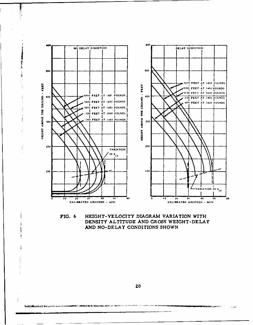
Height-velocity diagrams were first constructed from theexperimentally obtained data points. Various cross plots of velocity,altitude, weight and height-above-the-ground were then constructed andstudied to determine what kind of relationships, if any, existedbetween the many H-V diagrams. Information from these cross plots wasthen used to adjust the original fairings of the height-velocity curvesso that the curves then obtained provided the best fit with the datapoints and cross plotted points. The results herein presented exhibitlinear relationships which are quite similar to those obtained from thetesting reported in Reference 1. Since the test helicopter was quitesmall and utilized a sea level engine, the number of weights andcltitudes at which it was possible to obtain data was restricted, thussomewhat complicating the ability tv establish a confirmed relationship.These adjusted curves with experimental data points are shown in Figs.4 and 5. The variation with altitude and grnss weight is shown in Fig.for both no-delay and one-second delay conditions. The variation withaltitude for each of the two gross weights is shown in Fig. 7. Thevariation with gross weight for the density altitudes tested is shownin Fig. 8.

Since the density altitude spread for all the runs at any giventest site was larger than desired, an average density altitude for eachcondition of weight and collective pitch application was derived andutilized to facilitate data analysis. Test points could not be qualifiewith respect to their relative position about an H-V curve in accordancewith their test density altitude; i.e., outside the curve for higheraltitude and inside the curve for lower altitude. Other variables whichhad much greater effect on the data overshadowed the altitude variationeffects.

One exception to the data pattern developed in the 1600 lb. no-delacurve. This data showed a height-velocity diagram at sea level whichgave a critical velocity which was two and a half mph too low, whereasthe same data at 5000 feet showed a critical velocity which was one mphtoo high when referred to the rest of the data obtained. The 1450 lb.data with no-delay and one-second delay, as well as the 1600 lb.one-second delay data, checked out to provide plots of airspeed vsaltitude and airspeed vs weight which agreed and conformed to the patterFurther, the 1600 lb. no-delay data checked out in the low hover regime.The dotted lines on Fig. 5 indicate where these H-V diagrams would havebeen if these tests had been consistent with the rest of the data. Thisexception and deviation led to consideration of and investigation intodrag divergence possibilities. It was concluded, however, that thesesmall deviations are part of the scatter band of data which existed inthe project.

6

The data contained in Table I is a summary chart of the pertinentfacts taken from the time histories relative to all of the high hover andnear high hover points. In all cases of high hover or near high hover,stabilizing of the autorotative descent was instituted within 25 to 35 feetof descent following throttle chop. That is to say, aft longitudinal stickwas applied so that the aircraft started to arrest its nose down attitude,and in a very gradual manner this was continued so that maximum nose-upattitude occurred approximately two seconds prior to touchdown regardlessof the initial height above the ground. The touchdown speeds (VTD) appearto be of the same order of magnitude independent of altitude and weightwhen the entry is approximately at high hover. There appeared to be anincrease in the touchdown speeds as the entry speeds increased but thiswas not consistent for the points in the area of the critical speed (V c)and critical height (hcr). The vertical descent velocity followingsimulated power failure from high hover or near high hover increases asweight and density altitude increase. The rates of descent listed inTable I were the maximum rates of descent obtained and are consideredstabilized rates of descent. These maximum rates of descent occurred onan average approximately five seconds after throttle chop. As forwardspeeds Increa ed toward Vcr these rates of descent decreased accordingly.This is shown in Table II which lists runs obtained in the vicinity ofh crand Vcr. With few exceptions, whether entry was from high hover orin the "knee" area, the incremental vertical accelerattons followingsimulated power failure varied between +.5 and +.8 g's.

It is interesting to note that all high hover and near high hoverpoints developed load factors at ground contact of less than two. Thisis compared to all the data points taken in the vicinity of the "knee"(Vcr, hcr) wherein all the load factors at ground contact were well overtwo. This peculiarity would lead one to suspect that the high hoverpoints might be conservative. This consistent distribution of landingload factors is explainable, however, in that in all the high hover andnear high hover runs, the pilot was able to execute a full cyclic flare,thus building up sufficient rotor speed so that collective pitchapplication cushioned the impact. For those runs in the vicinity of andbelow the "knee", it was not possible to develop a full cyclic flarewith its consequent rotor speed build .jp, and the landing was made withthe application of collective pitch utilizing available rotor speed only.With the low inertia rotor system of the test aircraft it was not possibleto develop the required energy for low contact velocities without thevital contribution of cyclic flare.

One other factor entered into the picture with respect to the highhover and near high hover data. Directional control difficulties occurredimmediately after t,.rottle chop. These were the result of rapid rotorspeed decay and thus rapid tail rotor speed de,-ay, both of which areattributable to the low rotor inertia. The problem was most pronouncedat the higher altitudes and weight where power required tq hover washighest. This is discussed under "Pilot's Comments" in Appendix 2.

7

Figures 9 through 11 show a comparison of time history data for hig1hover, low hover, and the critical speed area for sea level versus highaltituda. The figures show that the control inputs and aircraft attitudtare quite similar and in some cases almost identical over the range ofaltitudes and weights. The comparison of the high hover and Vcr, hcr dalincludes 1600 lb. data at 5000 fe~t in order to show the effects of weigtversus altitude. The 1600 lb. data at 5000 feet is practically identicalto the 1450 lb. data at 7000 feet altitude.

Discusslon of One-Second Del&y

It was anticipated prior to the initiation of testing that, becauseof the low rotor inertia, a step might exist at the "knee" of the H-Vdiagram in transitloning from a no-delay maneuver to a one-second-delaymaneuver. It was decided, therefore, to conduct the project throughoutwich no-delay in collective pitch reduction and do some one second delaymaneuvers to ascertain what the effecL would be. The data obtainedutilizing a one-second delay in collective pitcl' reduction followingthrottle cut did show a marked step in the curve. This increase in entr)speed for a given height held throughout the upper boundary such that thOheight at high hover (hmin) was also markedly increased. In developingthe N-V diagrams and thus the cross plots and final relationships, it wasdesirable to treat the delay and no-delay data of the upper boundary asseparate 1i-V diagrams. Examination of the time histories of equal heightdelay and no-delay data revealed no specific characteristic differences.The rotor speed after a one-second delay felt off more sharply fromthrottle cut than the no-delay which evidenced a more gradual decay fromthrottle cut. The pilot apparently accomodated the more rapid rotorspeed decay through an increase in entry speed or in the case of hminthrough an increase in height. The relationship between Vcr and hminappears to be consistent independent of the time of collective pitchreduction.

Effects of Weight and Altitude

As previously discussed, H-V diagrams were individually drawn throuieach set of test points and then cross plots constructed of speed versusweight and altitude from which final N-V diagrams were diawn. Thecontrolling points of the H-V diagrams such as Vcr, hmin and hmax werethen cross plotted in a manner to define the H-V diagram relationships.

These cross plots are shown in Figs. 12 through 15. The high hoverheight, hmin, is shown to vary linearly with the square of the criticalspeed independent of weight, altitude and the time delay in collectivepitch reduction as shown in Fig. 16. A set of H-V diagrams resultingfrom these tests can be partially defined In terms of the criticalgoverning points on the H-V diagram which can be obtained from a set oflinear equations. These equations are basically identical to those ob-tained in Reference 1. The differences between these equations and

those of the previous tests are in the constants which define the slopesof these linear expressions. The height, hcr, must also be known inorder to properly locate the point Vcr, hcr. In the previous tests, hcrwas reported as essentially constant at approximately 95 feet. Thecurrent tests clearly indicate that hcr increases with weight and altitudeas shown on Fig. 6 by the dotted lines. Throughout the ranges of weightsand altitudes tested this height vAried from about eighty feet toapproximately one hundred feet. Inasmuch as the expression shown belowfor Vcr holds true for speeds at heights above and below the height forVcr for approximately forty to fifty feet as well, the shape of thefamily of curves is seen to be relatively constant in the area of the"knee". Therefore, selecting an average hcr of 90 feet would not effectthe construction or the H-V diagrams. No attempt mas made to establishan expression for hcr"

The equations shown below can also be used to determine thereduction in weight required for a constant H-V diagram as the altitudeis increased. This can be obtained by drawing a horizontal reference linethrough the intersection or the basic weight and sea level as shown onFig. 13. This is idpntical to the procedure developed in Reference 1except that since the constants of this data are greater, the percentagereduction of gross weight in lbs. per 1000 feet of altitude will also begreater.

Equations

1. Vcr a Vcr(te't) ' Cl AW + C2 &HD

where Vcr - critical velocity at a given weight and densityaltitude

Vcr(test) - critical velocity obtained through test

C, a dVc___

dW

C2 a dVcrdHD

9

2. hmax a hmay(test) + C3 A W + C4 AHD

where hmas a low hover height at a weight and density altitude

hmax(test) - low hover height obtained through testing

C3 a dhmax

dW

C4 a dhma_._

dHD

3. hgin K + C5 Vcr 2

where K a 3 constant (the hmin intercept)

C5adhmin

2dVcr

The constants of these empirical equations are applicable only tothe test helicopter as were the constants of Reference 1. It isinteresting to note, however, that both tests resulted in a set of linearexpressions In which only the constants were different. Further, a hriefcomparative examination of the data of both tests indicates othercorrelating factors. It appcars possible, therefore, that a set ofequations can be obtained by the application of a nondimensionalanalysis of the basic parameters and test results of the helicopter usedin this project and in similar projects of this program, which would beapplicable to all single engine, single rotor helicopters. Such ananalysis might determine whether H-V diagrams can be predicted ordeveloped over a range of weights and aititudes from single weight andaltitude test data. No attempt has been made to do this in this report.

10

V-W

CONCLUSIONS

Based upon :he tests of this small single rotor helicopter and ananalysis of the test results it can be concluded that:

I. The H-V diagrams for this helicopter at different weights andaltitudes form a family of curves for the altitudes and weights testedwhich are defined by a set of equations involving key points on the H-Vdiagram such as Vcr, hmin and hmax. These equations show that:

a. Vcr is a linear function of weight or altitude.

b. hmax is a linear function of weight or altitude.2

C. hmin is a linear function of Vcr

2. The height (hcr) for critical velocity (Vcr) increases over therange of weights and altitudes tested varying between eighty to one hundredfeet. Since the shape of the H-V curves are relatively constant in thearea of the "knee", a constant average height of ninety fePt for hcr can beassumed without destroying the family relationships of these curves.

11I I I I I I I I I I l

REFERENCES

1. W. J. Hanley and C. DeVore, An Evaluation of theEffects of Altitudeon the Heigh.t Velocitv Diarram of a StnRle Enrine Helicopter,Technical Report AUS-I, February, 1964.

BIBLIOGRAPHY

1. W. D. Jepson, Some Considerations of the Landinr ant Talfe-offCharacterlstics of Twin Ervtine Helicopters, Journal of AHS, Part I,October, 1962.

2. H. J. Rich, An Energy Absorption Safety Alighting Gear forHelicopter and VT.OL Aircraft, IAS Paper No. 62-16, January, 1962.

3. E. F. Kattenberger and M. J. Rich, An Investigation of HelicopterDescent and Landing Characteristics Following Power Failure.Journal of Aero Sciences, April, 1956.

4. Alexander Klemin, Principles of Rotary Wing Aircraft, Reprint AeroDigest, 1945.

5. A. Gessow and G. C. Meyers, Aerodynamics of the Helicopter,The MacIMillar Co., C 1952.

6. D. Donmasch, Elements of Propeller and Helicopter Aerodynamics,Pitman Publishing Company, C 1953.

12

• • m,~M i-iPMU i

4-

E'fl*IEIifi9E!

I- ' 11 1a

t I I f I I f f I I I rfr I fi F I I -. a I I i I i i I I I t

," .... U

HIM

""IIiI I I a I $ I4 Ilk v It a I i A a 9 A t s 1 9 z a 2 p s I r t~ a r r1

Si . . . ..... ....

sl a r s 0 2 ro t I t 1 t t 0 sI 2l i i K t a r t a t a 2

13

IJ~- - ~. <

C t 13 1 11 t r 9! OI f4-.

AI 1A1 A 'A I A '

0- ft .0. . I ...ll

S.. .. . .. .. . . . . . . . . . . . . . . . . . .- • •

. - o •

14

hmin

SAFE FLIGHT AREA

E::w (AVOID) :~:* .-

**. o I.

cr

VELOCITY

FIG. 1 TYPICAL HEIGHT-VELOCITY DIAGAAM

15

t iIi•.••,

• •,/2

S;?i•:A

!i/•i ,:•r

•,/i:•il : i i •• •'•iI

'•.i•-i¸ : /

S• ...... • .... .. N

S ,•ra-AZ • & sJ.~ .~.kJ& .~..

16

qI

2 0/

oz~ ~ hi1 -

- 04

w le

00

17

IA0 V)

004 z 400 00

in

Mu 06

b4

LIZI C- OVfOO 3HI ZAOQV 1HOtlIH 0R -

Xi X

__zk_ o

0' u

Lila MflOVD IH.L 2AOUV LHOIIH

I-- 18

~~~0C - 4~~~~~~~~~00 ____________________

LEG END.

FLIGHT FLIGHTNUMBER NUMBER

Soo 5Soo z

0 29

w I SECOND DELAY POINTS P

1 1 E AVERAGE H.AVLRAGE Ht D ODLY 0 T

NO DELAY 030 NO. DLAY Y 5000 FT.hi I SECOND DELAY .475 FT. NI SECOND DLY 50 Thi - 400 NO DELA

Ib. 400 NO0 ELA

a SECOND DELAY

SEN O N DELAY 0N 1me I ac

hi

IN SDE CO D D LAA.

I-300I 300

0

REQUIRED TO FIT _ _ _

FAMILY PATTERN

(SEE TEXT ONPAGES 6 AND 7)

m200 mzoo REQUIRED TO FIT_L~j FAMILY PATTERN

(SEE TEXT ONPAGES 6 AND?7)

be - 10''-0

0 10 20 30 40 s0 60 0 10 20 30 40 110 60

CALIBRATED AIRSPEED -MPH CALIBRATED AIRSPEED - MPH

FIG. 5 HEIGHT-VELOCITY DIAGRAMS - BASIC DATAHELICOPTER GROSS WEIGHT 1600 POUNDSTWO DENSITY ALTITUDES SHOWN

19

N - o DELAY CONDITION DELAY C ONDITION

7271 FEET AT >S OUNDS-

iF'

~40 69~ EETAr 5 POUNDS S0 -30 FEET AT 1450 POUNDSI

I

,p000 lET AT 1600 POUNDS

40 ;;o 6900 FEET AT 1600 POUNDS40 11 500 FEET AT 14S0 POUNDS

St I I i,

S,.00 FEET AT 1600 POUNDShi I I-300 FEET AT 14S0 POUNDS

30 Do -- 300

zoo 2 00

,,/IN\

10 - -100

- --- - -"aoo

100 VARIATIONTINN

0 10 20 30 40 50 60 0 30 20 30 40 s0 60

CALIBRATED AIRSPEED -4PH CALIBRATED AIRSPEED - MPH

FIG. 6 HEIGHT-VELOCITY DIAGRAM VARIATION WITHDENSITY ALTITUDE AND GROSS WEIGHT-DELAYAND NO-DELAY CONDITIONS SHOWN

20

.00 600 ..-GROSS WEIG'1T 1450 POUNDS GROSS WEIGHT 1600 POUNDS

00 775 FEET . I SECONDDLA

I I1

,,5300 FELT - I SECOND DELAY

So00p 6900 FEKET - NO DELAY So00 FEET -I SECOND DELAYt I I

5000 FEET- NO DELAY 5000 FEET- NO DELAY

1-00 FEET - I SECOND DELAY

-300 FEET -NO DELAY-475 FEET - I SECOND DELAY

-300 FEET - NO DELAY

hI~ 40 .400

z __ ___

o 0

300 '"I-300

0

x zoo \

I O' ,oo -

10 2C 30 40 50 60 0 10 zo 30 40 50 60

CALIBRATED AIRSPEED - MPH CALIBRATED AIRSPEED MPH

FIG. 7 HEIGHT-VELOCITY DIAGRAM VARIATION WITH DENSITYALTITUDE AND GROSS WEIGHTS OF 1450 AND 1600 POUNDSSHOWN-DELAY AND NO-DELAY CONDITIONS

21

0.o

40001__0

- - - 14S0 POUNDS NO DELAY (SOOO FEEl

1450 POUNDS - I SECOND DELAY

1640 POUNDS NO DELAY (-300 FEET) (I FEEI

i450 POUNDS I SECOND DELAY I.60 POUNDS -NO DELAY (\000 FEET)id -i00 FEET) J I I I"401600oPOUNDS I SECOND DELAY400 140E003 600 POUNDS NO DELAY (-300 FEET)

1160POUNDS I SECOND DELAY 2:(-475 FEET) 0

300 -00

--- - a-too - - -0o - -

100 -1 00 - - _ __

0 10 20 30 40 so 60 0 10 ,0 30 40 so 60CALIBRATED AIRSPEED - MPH CALIBRATED AIRSPEED MPH

FIG. 8 HEIGHT-VELOCITY DIAGRAM VARIATION WITHGROSS WEIGHT AND DENSITY ALTITUDE SHOYWN FORDELAY AND NO-DELAY CONDITIONS

22

w -

0000

000A. 0. 0.

- ~04o -fa

s~f3Jd03G "am ~ dln 3SON 'NO 39ON iv Nc amj walam'y IaYlg a3ds fO.lowi S3IUD03a S33IDX(103ariuj.zLiv Holld 1-ID:NY 31yid HSVIAI.

23

- 2 -- - - -w~

000 0

000

VSV

- - -- -04w

== ye

30111 H:Ilc 1N 31 0i Hlv

241

*LRtASRFOWLF STOPI) m,c fel of T" I 4SOU POt ND,, -3.-0 FEE FLIGOHT 46twol! TelT AtTil ct tLI_)I 1lo -fmmý 4S F11-L.70 F LG T )

w J

500*

0..

1, 0- -T-

TIESEOD

FI.1 OPRSNxFTM ITR

DAAFR O0OERPIT

-3o5

600~

m -I

14o 15F a-- 17

600

dV -

1 4 15161

WEGT 0 PUD

HEST AL ALTITDEDE00SFE

606

C max 013

[-,3 dW

- ~ 3 D00FEET D........ .......30

FEET NO DELAYý0 oooDELAY-0 1 0 50)0 fEET N__ DELAY

0 ----

0.1..... 6. '4014 is 16

WEIGHT - 100 POUNDS

FIG. 14 LOW HOVER HEIGHT (hmax) VERSUSAIRCRAFT GROSS WEIGHT FOR THERANGE OF TEST DENSITY ALTITUDES

SALTa0 00144 dHD

27•L

X o

0 I 05.

H D -ALTITUDE - 1000 FEET

FIG. 15 LOW HOVER HEIGHT (hmax) VERSUS TESTALTITUDE FOR THE RANGE OF TEST WEIGHTS

27

w

w- 0 U I-~>

v o

0 1-

NL o

- -1 -V

UN-10W- --OU 13- UIL 4) -H11 -3OI W)

2 8

APPENDIX 1

TEST AIRCRAFT SPECIFICATIONS ANDINSTRUMENTATION DETAILS

APPENDIX 1

TEST AIRCRAFT SPECIFICATIONS

Significant specifications of the test aircraft and its powerplantare as follows:

1. Powerplant: Lycoming Model HIO-360-AIA

a. Horsepower rating - 180 HP to 3900feet

b. RPM limitations - 2900 Maximum, 2700 Minimum

2. Weight, Cross:

a. Maximum certified - 1670 pounds

3. Service ceiling:

a. @ 1670 pounds - 14,000 feet

4. Hovering ceiling:

a. @ 1670 pounds - 7700 feet - in ground effect

b. @ 1670 pounds - 5300 feet - out of ground effect

5. Maximum speed:

a. Sea level - 87 MPH- IAS

6. General data:

a. Rotor diameter- 25.29 feet

b. Rotor disk area - 503 square feet

c. Rotor blade chord -. 562 feet

d. Blade twist - 80 washout

e. Airfoil section - NACA .0015

f. Number of blades - 3

p. Solidity ratio - .0424

h. Disc loading 1I 1670 pounds - 3.32 pounds/feet 2

i. Rotor inertia - 135.6 slug feet 2

J. Rotor System Configuration - articulated

k. Flapping Hinge Offset - 2.125 inches

1-1

TEST JAIiCR~rr SPECIFICATIONS CONTINUED

1. Engin, to main rotor ratio - 6:1

a. Rotor speed limitations *530 RPM Maximuma, 400 RPM Minimumi

l1.2

TEST INSTRUMENTATION

A brief description of the test instrumentation utilized for thisflight test program is as follows:

1. Airborne

The airborne quantitative information measured was:

a. Airspeed

b. Altitude

c. Rotor rpm

d. Engine rpm

e. Collective Stick Position

f. Cyclic Stick Position

g. Acceleration (verticad

h. Fuselage Attitude (pitch)

i. Angular Velocity (pitch)

J. Height (radar altimeter)

k. Instantaneous Vertical Velocity

1. Throttle Position

This information was recorded on an oscillograph. Figure 1-1 showsthe installation of the recording equipment and some of the basicinstrumentation within the cabin of the aircraft. Figure 1-2 points outthe location of some of the airframe instrumentation and exterioraccessories utilized for the control and accomplishment of the test.

2. Ground

Space position equipment utilized for tracking the aircraft isshown in Figs. l-3a and l-3b. Two photographic flight path analyzerswere utilized so as to augment each other's photographic capability.The phototheodo ite flight path analyzer, because of its limitedheight coveraige was used specifically for the low height-over-the-groundtests that involved primarily vertical movement of the helicopter. TheFairchild flight path analyzer was used primarily for flights thatInvolved high heights-over-the-ground and relatively large horizontalhelicopter movements. A sample photographic plate is shown in Fig. 1-4.

1-3

•e • • imn.......... nowt~ ma !2!•_ ... . .. ,,, ,.. ... .....

Neteoroloizlal equipment utilized for recording stmosphoricconditions during the flight tests is shown in Figs. 1-5s and 1-Sb.

The wind speed and direction recorder was a battery-opcrztedportable field instrument capable of recording wind speed from 3/4 mphto 10 mph and wind directions throughout 354 degree azimuth. Theequiptent's low threshold and high sensitivity permitted spontacnousand accurate measurement of small scale fluctuations in wind directionand velocity.

For measurinS atmospheric pressure, a portable precisionaneroid barometer with an indicating range capability of 1030 to 540millibars was utilized. The versatility and high accuracy of theinstrument made it ideal for use at all of the selected test sites.

Wet and dry bulb air teaperatures were measured with a portableelectrically aspirated psychrometer. These measurements together withaccurate pressure indications were the basis for accurate determinationof the density altitude at the time of testing.

1-4

RCORDIG'N

N; OSC ILLO G RAP H

0- fr

'-' OO CYC

FIG.~ ~1 G- AIBRE INTUMNATO

1-5

C-C

aax

N. I

C -6

10 ~ ~ ~ ~ ~ ~ ~ ~ Nc -mo ?I i l m1 11

AI

XNN

A. Faitrtheldot Flight Path Analyzer(MStill. Picture)

~~1-7

-7r-V

P"' OPP, 0

Al d~

A' 4 1I4.

NroAMoq # 'IL

:44 NY)Ul~flO . s ~'

41 INV

1-8

A. Wind Speed and Direction Sensors

7

B. ~ ~ ~ ~ ~ 6 Dat Cetr esuig n

'1 9

I

APPENDIX 2

PILOT 'S CO"QENTS

APPENDIX 2

PILOT'S COMMENTS

Introduction

The test pilot's ccomments relative to the various techniquesemployed in executing the simulated power failure landings, and hiscomments concerning the characteristics of the helicopter withrespect to the project are included herein for a better understandingof the material contained in this report. The commients are presentedin two basic forms. First, in the form of general commen's asprepared by the pilot from an overall point of view, and second, inthe form of questions and answers concerning specific areas of interest.

General

Final review of pilot techniques utilized, in the determination ofmaximum data points only for the height-velocity project, reveal thatfor each major area of the diagram a different technique is required.The determination of whether a point is maximum can be arrived at, inmost cases, by determining if proper entry conditions were adhered to,such as good control of airspeed maintained, full utilization of cyclicflare, and proper and maximum use of collective pitch resulting in atouchdown landing that meets the desired criteria established for thetest with regard to impact velocity. The areas of hmin, hmax, and thelow boundary require variations to the above and a description of thetechniques utilized in obtaining the maximum point in each area will bediscussed below.

hmin - The accomplishment and determination of a maximum point fromhmin is, in my opinion, the most difficult area encountered during theproject. Obtaining the one second delay, which should be strictlyadhered to for proper evaluation of the point, requires some concentra-tion coupled with determining that it is a true hover condition andthat the altitude is precisely maintained. The technique utilized inthis area is to obtain the airspeed required for an effective flare,accomplish the flare as near the ground as possible, allowing onlysufficient height above the ground to rotate to a level attitude andthen utilize remaining collective pitch. This technique results in alower impact velocity with regard to the test requirements, howeverthe maximum point has been established. Utilization of any othertechnique with this aircraft would increase the impact velocity,however, hmin would also increase.

hmax - These points were obtained by some reduction of collectivepitch following throttle chop and then increasing collective pitch tothe full up position just prior to touchdown.

2-1

1over 5ound.rv - The establishment of r maximum point in thisarea was determined by impact velocity and rotor energy. In the lowarea of this boundary where airspeed and altitude are insufficientfor a full effective flare, either a partial flare or none at all wasused. Utilization of collective pitch also varies as to whether itcan be completely reduced, partially reduced, or not reduced at allfollowing throttle chop. The most critical data point from thestandpoint of the pilot being able to utilize any type of techniqueto improve the condition occurs in the lc4 altitude and low airspeedarea. ThiL flight regime of approximately ten feet and fifteen milesper hour is where airspeed available is insufficient to flareeffectively and rotor ittertis is insufficient to hold the aircraftthrough the longer glide path which is caused by the airspeed.

In review of all data points, rough data only, it is my opinionthat the ability to obtain full utilization of a well coordinated cyclflare is the main determining factor in obtaining a maximum data pointThe proper application and utilization of full collective pitchcertainly is a strong factor in the data point also, however, theproper and full utilization of collective pitch will not establish themaximum obtainable data point unless the maximum effective flarepossible is obtained.

QUESTION AND ANSWER

1. Question -

Describe the loss of control at che high hover followingthrottle chop, both directional and pitching control.

Answer -

A. Directional control deteriorated in a ratio to the powerrequired for hover (gross weights and density altitude) and the amountof delay utilized in lowering the collective pitch. Pedal applicationwas considerable during the initial 100-150 feet of the dive that wasrequired to regain airspeed.

B. Pitching control problems occurred only when the rotorRPM was allowed to deteriorate very low or the gross weight of theaircraft and the steep angle of dive did not permit a rapid buildupof rotor RPM prior to the flare.

2. Question -

Is the above effect more pronounced at 1600 lbs. than at 145(lbs. or vice-versa?

2-2

Answer

The effect is more pronounced initially out of the hover cutat 1600 lbs., but becomes acceptable early in the dive. The 1450 lb.hover cut is marginally acceptable initially, however, some additionaldeterioration occurs during the early portion of the dive to regainairspeed.

3. Question -

Does it appear to be more serious at altitude or is it thesame for a given height above the ground appropriate to the altitude?

Answer -

It is more serious with altitude which is probably due to thepower required and higher rotor decay following throttle chop.

4. Question -

Under what conditions does the tendency to "fall thru" arise?That is, what transpires when the helicopter fails to respond to aflare?

Answer -

The perspective and feeling that the pilot gets when thehelicopter is "falling thru the flare" is that either the sink rate wasin excess of what he anticipated while higher above the ground, or thathe is in a down-wind or down-draft condition. The pilot at this time isquite certain that the flare will not stop the rate of descentsufficiently and therefore he will attempt to level the aircraft andapply collective pitch prior to impact or initiate a power recovery, orboth.

5. Qucstion -

Does the failure to respond to a flare in arresting the descenthave as an 'dded factor, the reduction in ability to level out (pitchingcontrol) or are they separate factors?

Answer -

It appears that the problem in leveling out is the result ofcollective pitch being applied in the flare, thus reducing rotor RPMand encountering a partial loss in longitudinal controllability, ascompared to operating with full rotor RPM until level.

2-3

6. Question -

In each of the various regimes of the H-V diagram, what seemsto be the moat important factor in achieving a minimum point on thediagram?

Answer -

A. hmin - Altitude in which to regain flare airspeed withoutresorting to an excessive dive angle. Directional control in someinstances adds to the altitude required to accompl!sh this.

I. "Knee" - Altitude to regain flare airspeed and build uprotor RPM and the rapidity of movement required by the pilot.

C. Lower Boundary - If sufficient altitude is still availablefor a slight dive and flare then the pilot reaction and movement timeis the most important factor. If altitude and airspeed is not availablefor flare then ground contact speed and proper use of remaining collect-ive pitch is the important factor.

7. Question -

What is the best technique from high hover or near high hover?That is, does the rate of descent increase with an abrupt lowering ofthe pitch over that which would be achieved at a slower more steadypitch reduction?

Answer -

I found that the best technique was a rapid reduction of collectivepitch either following a no-delay or one-second delay throttle chop. Thehigh hover rotor decay rate is a direct function of power required andwhile it might appear that initial descent is slower with a slow reductionin collective pitch, the rotor RPM has to be regained eventually by theuse of airspeed and flare.

8. Question -

What is the effect on control of these pitch reduction techniques?

Answer -

A one-second delay throttle cut followed by a slow collectivepitch reduction will bring rotor RPM to minimum red line or below, andthus result in some of the directional and longitudinal control problemsexperienced.

2-4

9. Question -

With respect to the upper boundary, how does the one-seconddelay affect the rotor speed decay?

Answer -

Proportionate to the collective pitch position required forthe power utilized in stabllizlrg on the particular point.

10. Question -

Does this delay contribute markedly to the loss of controldiscussed above?

Answer -

Proportionate.

11. Question -

What are the factors in the one-second delay which contributeto the marked increase in entry speed required to eFfect a landing?

Answer -

Loss of rotor RPM, some increase in airspeed required to regainthe additional loss of rotor RPM versus no-delay, and probably failureof the pilot to react instantly to desirable cyclic movements as someof his concentration is devoted to insuring that the delay time is quiteprecise. These would be fraction of a second movements and decisions,however, they could affect the determination of the maximum point.

12. Question -

What was most difficult about obtaining high hover data(h min. points)?

Answer -

A. Unstable air conditions is the prime factor.

B. Secondary, would be the stabilizing of the hover condition.I attempted to give consistent power conditions for the throttle chop,the radar altimeter made this a very difficult area. This is a conditionthat should be read very closely on the oscillograph (for both projects)because unless the pilot is conscientious to the program, he could makethe area of hmin look better than it is by being in a high powercondition initially &nd then reduce collective slightly Just prior tothe cut or at the cut.

2-5

• , ,, ,, ..... ..- . . .. . .

C. The decision at which time and position to abort theautorotation or decide that you might make it if everything canesout perfectly.

13. Question -

What was the criteria used by you to determine if a point wasmaximum at the time of execution; i.e., impact, control response andtime available, rate of sink, aircraft shudder, directional instability,etc.?

Answer -

You answered it! Some particular point on the H-V diagramwould have one of these factors associated with the determination ofa maximum point. The very least consideratici would be given toaircraft shudder. The majority of the maximum points were determinedby maximum utilization of flare, rotor energy and impact.

14. Question -

Did this criteria vary with the point being attempted; i.e;.,upper boundary, lower boundary, "knee"?

Answer -

Yes. Attempt was made, however, to utilize full benefit ofrotor energy and mayimum impact in the determination of all points ifat all possible.

15. Question -

What is your opinion relative to the effects of wind on thevarious areas of the diagram determination, particularly as it concernsthe 269B?

Answer -

A. In the area of hmin the wind factor is very important. Ifit is down-wind at the throttle chop point, it affects the attitude atthe cut and also 3ppears to add to the pilot's impression if anaccelerated sink condition. The wind condition at ground level, unlessabnormal, would not appreciably affect the hmin condition as this pointappears to be greatly affected by dive angle, time to regain airspeed,sufficient flare to build up rotor RPM, and time required to levelaircraft following flare.

2-6

B. Head wind benefits the diagram 'n the area of the "knee"and the lower boundary. I am not certain, however, that a quarteringwind to the direction of a landing is exactly the same relationshipthat would result from a wind vector problem. I recall havingdifficulty with some points which had a plus wind component and yetwere of the crosswind or quartering wind type.

C. Cross or gusty wind conditions definitely affected thevery slow airspeed points as it resulted in considerable pedalapplications in order to stabilize on a given condition for the timerequired to fly from the radio link actuation to the desired point ofthrottle chop.

16. Question -

Do you believe that any other landing or touchdown attitudewoul, materially affect the size or shape of the H-V curve?

Answer -

It is conceivable that a nose high landing might reduce thesihe or change the shape of the H-V curve, however, some of the touch-downs were of a fairly high impact type and I am positive that thesewould have still been hard with the nose high technique and thus resultin some type of failure. In the area of the lower boundary (air taxi)this technique would definitely not be utilized, as no benefit couldbe derived from # flare at such a low airspeed, and sufficient rotorenergy to cushion a nose high landing does not exist at that time.

17. Question -

Did you experience any difficulty in adjusting to the variousdensity altitudes? Did a large change in altitude affect yourperformance initially at the new altitude!

Answer -

A. Yes. I initially did not believe that the H-V curve at7000 feet would be as completely defined as it w3s. I felt that thehigh entry speeds would be prohibitive to oktaining many points. It wasmy belief that the sea level testing would not represent as much of areduction In airspeed and altitude as it eventually did.

B. Yes. Obtaining the mental preparation for operating in anarea that had not previously been conducted under normal certifisationprograms resulted in a cautious approach and some pre-planning of theexpected escape path in the event an unforeseen problem area arose.

2-7

C. The most difficult area to adjust to, however, was theunstable air conditions that existed during the repeat flights atBishop and the high hover points at Fresno. In many instances, pointsbecame more difficult in these conditions than they were whenpreviously completed from lower altitudes and slower airspeeds.

2-8

APrENDIX 3

SU?10ARY OF HEIGHT-VELOCITY DIAGRAM FLIGHT TEST DATA

P L r.A TA AZrV.? I 7iýy IA '<?No. W.,. 96 04 ar% W17 A.~.~ C,~ v- A.1

19 2 10"13 I151 'NX) -3,1 72.C 33.1 16.4 3,45 0, a7 (319 5 10/13 1438 485,o 42.9 4,0 3.).3 22.9 2 09 0.1910/9 6 10/3 11435 ,o +2,5 V.5 30.5 16.2 2.0o' 0.2S a 13 i451 5#00 .3.5 38.0 30 6 13 8 2,80 0, 119 11 10/13 1455 5350 41.1 192.0 25.9 21.0 2.65 0.52

19 12 10/13 1451 540v +2.1 196.5 23.7 19.9 2.54 UW, (2)19 13 10/13 1449 5400 +2.6 dil.o 22.4 20.7 1.65 0.2019 14 10/13 1447 5400 -0.4 307.0 -0.4 17 4 1.83 0.1919 20 10/13 2451 5600 42.6 14.2 0 Umx 2.62 0.15 (1)19 2i 10/13 1450 5600 -1.3 11.6 1.2 2.9 2.91 0.27 (I)19 22 3'V1 3 1438 5750 +1.5 18.0 13.7 10.7 3.53 n.47 (3)20 ill 10/14 1596 5300 42.7 39 .0 8.3 14.0 IrK o.o6 (2)

21 3 10/15 15r#8 450o 41.3 "50.0 A2.0 17.1 2.20 0.0621 6 10/15 16o9 4700 +3.6 200.0 36.8 19.? 2.14 0.1121 9 10/15 1598 4850 .4.0 251.0 31.9 15.6 1.87 0.1422 3 10/16 1600 4300 +2.6 101.0 42,9 18.7 2.87 0.1522 4 10/16 1597 4300 .1.9 63.5 44.9 18.8 2.50 0,1422 7 10/16 1594 4,500 43.2 306.0 26.6 12.1 1.65 0.1422 10 10/16 1602 5150 +1.4 314.0 29.2 15.9 1.59 0.1522 11 10/16 1599 5200 *0.7 337.5 20.6 12.5 1.74 0.1522 13 10/16 1601 5300 +0.9 394.0 16.5 11.4 2.32 0.0722 15 10/16 160o 5450 -2.6 445.0 -2.4 13.3 1.56 0.1225 10 10/20 ,.;9 4900 +4.7 97.5 51.9 20.2 2.60 1.18 (3)25 11 10/29 1592 4950 +3.1 278.0 36.8 14.8 1.67 1.4725 12 10/20 1590 5000 +2.8 189.0 44.8 ,• ' 1.59 1 C4

13 10/20 1608 5100 +4.2 396.0 23.5 12.3 1.87 1.40Z, A•

1 , l _5-.. ~ -• •" !. 1.t'9 1.1225 15 10/20 1598 5200 .4.3 338.0 29.4 11.0 1.70 0.7726 10 10/21 1448 4500 +1.2 ,'0.0 20.7 13.3 2.10 1.0826 12 10/21 1446 5225 41.0 15.0 ?9.5 M"N 1.85 0.27 f1)26 15 10/21 1451 5650 -0.1 99.0 43.3 17.9 2.04 0.8728 2 10/23 1451 50oo 4.6 93.5 35.5 28.6 2.45 0.262I 5 10 /23 1451 5250 43.1 108.5 39.1 18.6 2.29 0.1328 8 lO/23 1Wo0 5300 -'4.7 227.5 23.3 19.7 1.98 0.i2

1l" 10 20/23 14,r 5400 "3 9 346.0 6.4 19.1 1.83 0.1928 11 10/23 145? 5350 44.8 323.0 5.7 V1.1 i.5(, 0.1328 13 10/23 1447 5•00 o44.2 412.0 8.5 17.5 1.51 0.6ý (2)C1 2c/? 3 14153 550r .3.3 415.0 3.0 11.5 1.01 T1j?, (?)28 16 101123 i 4r 5500 ý1.2 136.0 36•.4 30.7 3,46 1.00 (3)"3 10/25 1599 47C00 40.8 e 40.4 4C. 5 C.5 , 9 .. 1'4

8 10/25 15)9 4900 43.3 ]'.0 31.9 18.5 2.93 D.1V,S 10 10/'25 1594; oo (O5.0 10.0 22.8 22.0 2.16 0.2216 11 l0A/2; 1(,8 5100 -0.8 /1"r). 0 40.' 14.8 1.63 0.27

3-1

S9 1 7/'25 16) "3 -1.9 4C4.0 -0.37 11.4 1.53 0.944IA 1C.25 V)Cý , 50 -0.8 478.0 0.6 11.3 1.54 0.79

29 15 10/25 16o5 5M .1.5 ,432.0 4.6 14.6 1.73 0.18719 19 10/25 1605 5300 40.7 10.5 0 ,*M 2.60 0.49r) 2 1c/25 > 1600 5350 -2.0 9.1 10.0 un 1.94 0.1630 2 10/"5 1455 5700 40.8 325.0 2.0 22.1 1.60 0.133c 14 1c/25 1447 580 0 278.0 18.0 10.3 2.06 0.1535 5 10/31 1445 f2r": +2.5 12.4 ý2.3 2.3 2.58 0.2635 6 10/31 1444 665o +2.5 12.0 2.3 2.3 2.80 0.2535 9 10/31 11447 675.0 +2.6 11.2 12.1 i.:.9 2.0! 0 1735 11 10/31 1443 6750 42.7 11.6 18.9 17.1 2.33 0.1636 7 11/3 1449 6550 +2.5 308.6 20.5 tfl 1.i4 0.i336 9 11/3 1444 6600 +1.7 187.5 32.4 UNK 1.78 0.0636 lA 11/3 1456 710) -0.7 150.0 40.3 19.1 2.11 0.1536 16 11/3 1448 7200 -0.9 430.0 0.27 9.6 1.51 0.1936 18 11/3 1450 7400 .1.4 510.0 2.5 11.1 1.5 0.8237 2 11,/A 1452 6550 -3.9 195.0 33.8 18.1 2.3i 0.137 4 11/A 1455 66mO -0.2 265.0 24.2 17.8 1.49 0.5337 5 11/4 1452 6600 +4.3 354.0 16.8 15.0 1.55 0.1937 6 11/4 144.8 6600 .0.9 106.0 43.3 19.4 2.43 o.2.637 9 11/4 1446 6650 +1.8 51.0 36.8 18.7 E.49 0.1437 12 11/A 1450 6900 +2.3 19.0 30.9 16.1 2.37 0.1037 14 11/4 1445 7000 +4.1 76.0 38.5 19.6 2.11 0.1437 i1 11/4 1445 710O +1.8 95.5 45.4 25.4 2.46 1.0037 20 11/4 1451 7250 .3.3 375.0 7.0 13.9 1.48 0.2137 23 11/4 1hrl 7300 -1.8 312.0 249.4 15.1 1.34 1.1039 2 11/6 1450 4800 +2.6 152.0 29.3 20.8 2.30 0.1739 8 11/6 144 4950 +2.6 246.0 Z2.9 17.4 1.80 0.1540 2 11/7 1451 +3.7 13.5 14.0 15.5 2.50 0.2-941 2 11/11 1454 3900 +3.0 21.7 24.4 19.2 1.81 0.1841 3 11/11 1451 3950 +1.4 2e.5 19.8 23.8 2.03 0.1341 5 11/11 1450 4150 -0.9 252.0 13.9 12.1 1.75 0.15Al 6 11/11 1447 4250 +1.4 251.0 11.5 14.1 1.72 0.1041 8 11/11 1450 4450 +3.1 143.0 24.9 23.3 2.41 0.0741 11 11/11 1443 4hoo +1.0 3;1.0 2.5 14.8 1.31 0.11

106 0 11/17 1",s8 -450 +3.6 100.0 23.6 13.4 2.26 0.14

S13 11/17 1454 -300 -1.5 263.0 0.2 11.4 1. 4 0.1246 14 11/17 1450 -350 -0.9 270.0 3.9 9.4 1.54 0.1046 15 11/17 14,47 -350 -1.4 255.0 4.9 10.8 1.62 0.1246 16 .:/,1 1•45 -4w +2.5 248.0 5.4 13.4 2.03 0.1246 19 11/17 1446 -350 +0.2 72.0 22.3 13.7 1.78 0.1346 24 11/17 1454 -350 +1.9 19.3 0 Um 3.27 0.2846 27 11/17 1449 -350 +2,2 26.0 81.2 Um 1.73 0.15

3-2

FLT. AUX DA rE AIRRc.P? DI." rY W cK.. L.AX' : I IY0!NO. NO. 1)64 3R" WT. ZtI't J! ý 7-"ffr ý " Vý -. " ?!

48 11 11/19 1149 -4!wo +2.2 .o0.3 13.3 9.9 1.97 O.C148 11 11/19 1443 -00 .4.0 &.82 •2•. M 2.03 0.10 (149 4 11,/19 1604 .300 42.50 16.0 3.3 1.) P.72 0.2049 7 11/19 1596 -300 -0.26 25.3 11.4 11.4 3,10 0.1119 10 11/19 1599 -100 +0.5.e 26.7 22.3 15.f 2.141 0.1919 13 11/19 1604 -250 41.6 53.6 26.3 TAM 2.81 o.i1 (1)50 3 11/-'0 1148 -700 +2.3 49.0 26.3 19.1 1.93 0.1650 6 11/20 1247 -650 .1.2 61.0 2e.3 186. 2.63 3.1750 7 11/20 1445 -650 -0.9 201.0 10.1 11.11 1.97 0.0950 8 11/20 11144? -550 .1.1 200.0 11.4I 13.2 1.78 0.1350 10 111/0 1451 -450 +2.6 230.0 10.5 16.) 1.39 0.0!50 16 11/20 1449 -350 4i.7 310.0 3.0 17.7 1.41 0.8650 19 11/n0 1451 -450 43.2 150.0 24.7 16.9 1.55 0.1453 6 11/23 1604 -300 -2.0 100.0 25.6 173 2.72 0.1854 3 11/214 15-96 +11O 41.7 198.0 12.3 20.0 1.91, 0.1456 1 11/30 16oo -550 +4.,; 72.0 26.3 23.6 2.47 0.1156 7 11/30 16o1 -500 +1.9 153.0 22.6 18.11 2.80 0.1356 10 11/30 1605 -350 .1.6 213.0 5,8 12,7 2.11 0.1156 11 11/30 1602 -250 -3.0 250.0 10.6 18.4 1.41 ').0856 23 11/30 16o4. -50 .4.1 290.0 41.9 19.41 1.81 0.1256 17 11/30 1596 -50 +3.9 112.0 32.3 22.9 2.70 0.9757 1 12/2 1607 4100 +1.9 97.0 37.3 19.6 3.25 1.0258 2 1212 1453 .100 +0.0 116.0 20.0 15.0 2.53 0.1158 3 -1/2 1450 "-400 -2.5 W1O. 16.4 18.7 2.32 0.1458 4 12/2 1454 4500 .2.4 55.0 25.6 17.6 P.26 0.08

1) 12,/2 11451 ý 4w .2.2 ýI.O 21.9 WO. 0 2.320.A58 6 12/2 1450 +500 -0.8 19.5 8.1 9.6 2.20 0.0959 3 12/4 1447 -50 +1.3 1014.0 30.5 15.5 2.02 0.9059 1 12/4 1454 -50 41.6 98.0 29.8 22.0 2.50 0.9659 5 12/4 1451 -50 +0.95 193.0 21.0 20.2 1.93 0.8059 6 2'`1% 1457 -50 +1.11 200.0 18.6 13.9 2.52 0.8759 9 12/4 1453 -50 +2.9 253.0 31.1 17.3 1.55 0.8059 10 12/4 1450 -50 +2.85 245.0 11.1 19.3 1.72 1.1061 3 12/6 595 -1000 41.8 26-.O 16.5 22.7 1.31 1.0061 4 12/6 160'. "950 +1.9 262.0 18.6 20.5 ý.C2 0.9161 5 12/6 1598 -900 42.9 252.0 17.3 21.6 1.36 1.0062 1 12/6 1452 100 +2.0 19.0 2.0 3.6 3.37 0.24

Notes 1. Data obt•lnod from CocIllograph omnl

2. Deta obtalne•d rul Photographlo Anelysis only

3. Rear arose tub* yield*d

3-3