Improving SAT Solvers by Exploiting Empirical

Characteristics of CDCL

by

Chanseok Oh

A dissertation submitted in partial fulfillment

of the requirements for the degree of

Doctor of Philosophy

Department of Computer Science

New York University

January 2016

Thomas Wies

c© Chanseok Oh

All Rights Reserved 2016.

Dedication

To all the great minds in computer science, with respect.

iv

Acknowledgments

I would like to thank my advisor, Thomas Wies, and my former advisor, Ben-

jamin Goldberg, for their great mentorship and sincere support throughout my

PhD years. I would also like to thank the other members of my thesis committee

for their time and feedback on this thesis: Clark Barrett, James Ezick, and Laurent

Simon. This work owes a great deal of debt to all the great researchers working

in the field of SAT. I would like to thank particularly the authors of MiniSat and

Glucose: Niklas Een, Niklas Sorensson, Gilles Audemard, and Laurent Simon. At

the start of everything was Sangkon Choi, without whom I would not have been

in the graduate program. Lastly, I would like to extend my heartfelt gratitude to

my family and friends for their overwhelming display of love and support.

During my PhD program, I have been fortunate to receive full financial supports

that allowed me to focus only on conducting research. The Graduate School of Arts

and Science at New York University has been generous to offer me the extensive

full funding support through the Henry M. MacCracken Fellowship Program. I

am also greatly indebted to Thomas Wies who provided financial support to me

in the last years of my PhD program. As a result, this thesis work was supported

by the National Science Foundation under grant CCF-1350574.

v

Abstract

The Boolean Satisfiability Problem (SAT) is a canonical decision problem orig-

inally shown to be NP-complete in Cook’s seminal work on the theory of com-

putational complexity. The SAT problem is one of several computational tasks

identified by researchers as core problems in computer science. The existence of

an efficient decision procedure for SAT would imply P = NP. However, numerous

algorithms and techniques for solving the SAT problem have been proposed in

various forms in practical settings. Highly efficient solvers are now actively being

used, either directly or as a core engine of a larger system, to solve real-world prob-

lems that arise from many application domains. These state-of-the-art solvers use

the Davis-Putnam-Logemann-Loveland (DPLL) algorithm extended with Conflict-

Driven Clause Learning (CDCL). Due to the practical importance of SAT, building

a fast SAT solver can have a huge impact on current and prospective applications.

The ultimate contribution of this thesis is improving the state of the art of CDCL

by understanding and exploiting the empirical characteristics of how CDCL works

on real-world problems. The first part of the thesis shows empirically that most

of the unsatisfiable real-world problems solvable by CDCL have a refutation proof

with near-constant width for the great portion of the proof. Based on this ob-

servation, the thesis provides an unconventional perspective that CDCL solvers

can solve real-world problems very efficiently and often more efficiently just by

maintaining a small set of certain classes of learned clauses. The next part of the

thesis focuses on understanding the inherently different natures of satisfiable and

unsatisfiable problems and their implications on the empirical workings of CDCL.

We examine the varying degree of roles and effects of crucial elements of CDCL

based on the satisfiability status of a problem. Ultimately, we propose effective

vi

techniques to exploit the new insights about the different natures of proving satisfi-

ability and unsatisfiability to improve the state of the art of CDCL. In the last part

of the thesis, we present a reference solver that incorporates all the techniques de-

scribed in the thesis. The design of the presented solver emphasizes minimality in

implementation while guaranteeing state-of-the-art performance. Several versions

of the reference solver have demonstrated top-notch performance, earning several

medals in the annual SAT competitive events. The minimal spirit of the reference

solver shows that a simple CDCL framework alone can still be made competitive

with state-of-the-art solvers that implement sophisticated techniques outside the

CDCL framework.

vii

Contents

Dedication . . . . . . . . . . . . . . . . . . . . . . . . . . . . . . . . . . . iv

Acknowledgments . . . . . . . . . . . . . . . . . . . . . . . . . . . . . . . v

Abstract . . . . . . . . . . . . . . . . . . . . . . . . . . . . . . . . . . . . vi

List of Figures . . . . . . . . . . . . . . . . . . . . . . . . . . . . . . . . . x

List of Tables . . . . . . . . . . . . . . . . . . . . . . . . . . . . . . . . . xi

Introduction 1

1 Background 8

1.1 Boolean Satisfiability . . . . . . . . . . . . . . . . . . . . . . . . . . 9

1.2 DP . . . . . . . . . . . . . . . . . . . . . . . . . . . . . . . . . . . . 15

1.3 DPLL . . . . . . . . . . . . . . . . . . . . . . . . . . . . . . . . . . 16

1.4 CDCL . . . . . . . . . . . . . . . . . . . . . . . . . . . . . . . . . . 20

1.5 Machine Configurations . . . . . . . . . . . . . . . . . . . . . . . . 37

2 Learned Clauses and Industrial SAT Problems 38

2.1 Learned Clause Management . . . . . . . . . . . . . . . . . . . . . . 40

2.2 Low-LBD Learned Clauses . . . . . . . . . . . . . . . . . . . . . . . 44

2.3 Evaluation and Discussion . . . . . . . . . . . . . . . . . . . . . . . 47

2.4 Clauses and Proofs . . . . . . . . . . . . . . . . . . . . . . . . . . . 61

viii

3 Satisfiability and Unsatisfiability 66

3.1 Background . . . . . . . . . . . . . . . . . . . . . . . . . . . . . . . 69

3.2 Satisfiability and Unsatisfiability in CDCL . . . . . . . . . . . . . . 73

3.3 Refinement on Learned Clause Management . . . . . . . . . . . . . 102

3.4 Concluding Remarks . . . . . . . . . . . . . . . . . . . . . . . . . . 104

4 COMiniSatPS 106

4.1 Introduction . . . . . . . . . . . . . . . . . . . . . . . . . . . . . . . 110

4.2 Patch Descriptions . . . . . . . . . . . . . . . . . . . . . . . . . . . 111

4.3 Experimental Evaluation . . . . . . . . . . . . . . . . . . . . . . . . 117

Conclusion 120

Bibliography 123

ix

List of Figures

2.1 Average LBD and no. learned clauses by Glucose . . . . . . . . . . 45

2.2 Cactus plot of Glucose and the modified solvers on SAT instances . 54

2.3 Cactus plot of Glucose and the modified solvers on UNSAT instances 55

2.4 Cactus plot of Glucose and the modified solvers on SAT instances . 57

2.5 Cactus plot of Glucose and the modified solvers on UNSAT instances 58

2.6 Comparison of runtimes: with and without database reduction . . . 62

2.7 Difference in no. conflicts: with and without database reduction . . 63

3.1 Comparison of runtimes on 69 SAT instances . . . . . . . . . . . . . 76

3.2 Comparison of runtimes on 66 UNSAT instances . . . . . . . . . . . 77

3.3 Difference in no. conflicts (%) on 69 SAT instances . . . . . . . . . 78

3.4 Difference in no. conflicts (%) on 66 UNSAT instances . . . . . . . 79

3.5 Cactus plot of solvers with different core LBD limits on SAT instances 83

3.6 Cactus plot of solvers with different core LBD limits on UNSAT

instances . . . . . . . . . . . . . . . . . . . . . . . . . . . . . . . . . 84

x

List of Tables

2.1 Different LBD limits for core learned clauses . . . . . . . . . . . . . 51

2.2 Different size limits for core learned clauses . . . . . . . . . . . . . . 56

3.1 No. solved instances with different LBD core limits . . . . . . . . . 81

3.2 Luby vs. Glucose restarts . . . . . . . . . . . . . . . . . . . . . . . 91

3.3 Luby vs. Glucose restarts . . . . . . . . . . . . . . . . . . . . . . . 92

3.4 Random decision variable selection . . . . . . . . . . . . . . . . . . 97

3.5 Different variable decay factors with MiniSat HACK 999ED . . . . 98

3.6 No. solved instances with new hybrid techniques . . . . . . . . . . . 100

4.1 Performance comparison of solvers at different stages of patch ap-

plication . . . . . . . . . . . . . . . . . . . . . . . . . . . . . . . . . 117

xi

Introduction

The Satisfiability Problem

The Boolean Satisfiability Problem (SAT) is to determine whether a given

Boolean formula can be made to evaluate to true by assigning Boolean truth val-

ues to the variables in the formula. SAT is the canonical decision problem originally

shown to be NP-complete in Cook’s seminal work on the theory of computational

complexity [9]. The problem is one of several important computational tasks iden-

tified by researchers as core problems in computer science [10]. Being one of the

most important problems, SAT has been widely and extensively studied from di-

verse perspectives, both theoretically and practically, resulting in an abundance of

literature. The existence of an efficient decision procedure for SAT would imply P

= NP from the complexity point of view. That SAT is NP-complete also implies

that we cannot expect to solve every SAT problem efficiently (unless P = NP).

Nevertheless, numerous algorithms and techniques for SAT have been proposed in

various forms to tackle SAT problems in practical settings. Highly efficient SAT

solvers are now routinely being used, either directly or as a core engine of a larger

system, to solve problems that arise from many application domains: Software and

Hardware Verification, Model Checking, Electronic Design Automation, Artificial

Intelligence, Synthesis, Planning, Bioinformatics, etc. Due to the practical impor-

tance of SAT, building a fast SAT solver can have a huge impact on current and

prospective applications and facilitate research advancements in dependent fields.

The focus of this thesis is on practical SAT research, i.e., solving real-world

SAT problems with SAT solvers that implement the framework of Davis-Putnam-

Logemann-Loveland (DPLL) [12] extended with Conflict-Driven Clause Learning

1

(CDCL) [4, 5]. In this thesis, we identify and analyze several interesting empirical

characteristics of these SAT solvers on real-world SAT problems. Ultimately, we

propose effective methods to improve the performance of CDCL by exploiting those

empirical characteristics.

We first emphasize that all the arguments in this thesis are applicable only to

real-world industrial problems. This is an important point to make so that readers

without sufficient expertise in SAT are not misguided to believe that the argu-

ments would hold universally. Specifically, the thesis excludes hand-made hard-

combinatorial SAT problems in discussions that also have been of interest to SAT

researchers. Such crafted problems often exhibit similar properties to real-world

problems. In fact, the distinction and classification between real-world problems

and crafted problems is not always clear. CDCL solvers usually work very well on

crafted problems too, and thus are the right choice of solvers in general. However,

there are many pieces of evidence that CDCL solvers do show different behaviors

on real-world problems and crafted problems. For some artificially crafted prob-

lems, it is known that CDCL solvers are inherently inefficient (e.g., pigeon-hole

problems) [23, 22, 24, 25]. We note that other types of solvers besides CDCL (e.g.,

local search algorithms) have been shown to be reasonably effective on certain

crafted problems in past competitions.

History and State of the Art of SAT Solvers

Contemporary SAT solvers implementing the DPLL framework are always ex-

tended with CDCL. For this reason, these solvers are usually called CDCL SAT

solvers. Very often, the term ‘SAT solver’ is used synonymously with the term

‘CDCL solver’ especially in practical settings because of the popularity and the

2

remarkable efficiency of CDCL in applications. However, it is worth noting that

there exist other approaches to solving SAT problems in practice besides DPLL.

Particularly, Binary Decision Diagrams (BDD) [7] have been studied extensively

and are still being used successfully in many applications. However, the currently

dominant method for practical SAT is DPLL due to its unmatched efficiency and

performance in solving real-world problems. Historically, DPLL solvers first gained

traction when the solvers were successfully applied in Bounded Model Check-

ing [28] as a replacement for BDDs and demonstrated remarkable performance

that extended the capability of hardware verification tools [71]. Modern DPLL

SAT solvers are now in mass industrial use and can tackle huge real-world prob-

lems with millions of variables. This is very surprising when one considers that

SAT is NP-complete. This empirical evidence indicates that industrial problems

do not exhibit worst-case behaviors in practice. However, readers should be aware

that, although DPLL solvers are incredibly efficient for real-world problems, they

show very poor performance on randomly generated SAT instances. Other types

of solvers than DPLL (e.g., Stochastic Local Search algorithms [8]) should be used

to tackle random SAT, which is another distant research area that brings in totally

different lines of arguments.

The basic DPLL algorithm without CDCL was first introduced in 1962 [12].

The algorithm was a refinement of the earlier Davis-Putnam algorithm (DP) devel-

oped two years earlier by a subset of the same authors [11]. However, the SAT prob-

lem was mainly of theoretical interest at the time, and polynomial reduction to it

was a tool to show the intractability of any new problem [3]. The landscape changed

far later in 1996 when CDCL was introduced to DPLL by the solver GRASP [4, 5].

CDCL has revolutionized practical SAT research, sparking a proliferation of the

3

development of very efficient SAT solvers. Since then, the performance of SAT

solvers has been improved by several orders of magnitude. The progression of SAT

research is one of the success stories in computer science [52, 99]. Some of the

most influential solvers that appeared after GRASP to date are Chaff [6], Min-

iSat [2], Glucose [3], and Lingeling [74]. Until recently, SAT solvers continuously

achieved substantial performance improvements each year. What is remarkable

is that most solvers retained the relatively simple structure of DPLL with CDCL

despite their impressive performance. As a most notable example, the critically

acclaimed MiniSat has made tremendous contributions to the advancements of

SAT research. Such contributions were possible because MiniSat functioned as a

“platform” that researchers could use to describe and concretize their ideas. Had

it not been for MiniSat, we might have not achieved the current state of SAT re-

search. What made MiniSat a “platform” was its very compact implementation of

only minimally necessary components as well as its top-notch performance. It is no

wonder that most state-of-the-art SAT solvers today have evolved from MiniSat.

(However, Lingeling is a notable exception.) Very recently, however, the degree of

performance improvements of SAT solvers has declined significantly. This decline

and the ensuing struggle for making further advancements may be responsible for

the recent spawn of SAT research into a wide spectrum of diversified and orthog-

onal directions: application of machine learning [72, 69, 70], intermittent formula

simplification (inprocessing) [21], attempts to exploit structured properties of in-

dustrial instances [13, 14, 15, 16], symmetry breaking [17, 18], shifting of focus

onto parallelization [109, 110, 52], etc. One of the common characteristics of these

recent works is the high complexity in both theory and implementation. These

works are also independent of each other, attempting to make improvements by

4

following completely different approaches. One reason that these works cannot

be interrelated to each other is that they are also independent of and external

to DPLL. In fact, for the past few years, what is considered “state-of-the-art” in

terms of only DPLL has not seen much change, with some minor variations at

best bringing no clear benefit. This disconnection and diversification among SAT

researchers may imply that the community is now struggling to make fundamental

changes to the highly optimized and matured state of DPLL and CDCL for further

innovations. Moreover, the complex and diverse nature of recent works resulted in

most solvers evolving to have very complex and large implementations compared

to the old solvers with the simple DPLL structure. In appearance, today’s com-

plex solvers do seem to outperform solvers of the past. Nevertheless, despite these

numerous efforts, it is still true that the rate of performance improvements has

been stagnating.

Thesis Contribution and Organization

At the highest level, the thesis improves the state of the art of DPLL by exploit-

ing empirical characteristics exhibited by the current state of SAT solvers. The

thesis solely focuses on the core DPLL structure where concrete advancements have

been stagnating recently. We shall see that old solvers with only the simple DPLL

structure can be rectified with small changes to achieve competitive performance

with any state-of-the-art solvers that implement complex features outside DPLL.

This result effectively proposes a new standard for DPLL and proves that the cur-

rent state of DPLL is not mature. Particularly, we achieve the improvement on

the state of the art with fresh and unconventional approaches, which subsequently

provide new insights on the empirical characteristics of SAT solvers. A detailed

5

breakdown of the contributions are provided below where we explain together the

organization of the thesis:

Chapter 1 serves as a preparatory chapter that provides the background nec-

essary to make the thesis self-contained. This chapter includes a brief history of

practical methods for SAT starting from the Davis-Putnam algorithm, where em-

phasis is given to the current state of the art. Essential elements of DPLL and

CDCL, and several components of typical SAT solvers are explained in detail.

Chapter 2 presents and advocates an unconventional perspective on the lemmas

(i.e., learned clauses) of an input theory (i.e., a SAT formula) that CDCL deduces

while solving a SAT problem. Specifically, this chapter provides data and analysis

showing that the majority of the lemmas learned by CDCL are not useful for

deriving a proof of unsatisfiability for real-world problems in terms of actual solver

performance in general. In addition, we show that an unconventionally small

fraction of “simple” lemmas (i.e., of a very high quality by certain criteria) is

enough to solve real-world problems fast in practice. This observation leads to

the hypothesis that current CDCL solvers are severely limited in that they are

incapable of efficiently deriving a sophisticated proof of unsatisfiability, or that the

only problems CDCL solvers can tackle efficiently are those problems that have a

short proof that can be easily constructed out of simple lemmas. In fact, we show

that most of the real-world problems that CDCL solvers can tackle efficiently have

a near-constant width1 for the great portion of a proof.

In Chapter 3, we improve the state of the art of DPLL by exploiting the dif-

ferences of DPLL when searching for a satisfying solution and deriving an unsat-

1In a formal context, the width of a resolution proof is defined to be the maximal size of anyclause in the proof [40]. Here, we extend the notion to include the LBD [3] of any clause inaddition to the size.

6

isfiability proof. This chapter gives partial explanations to the difference in terms

of the workings of some of the most important elements in CDCL: the effects of

search restarts and the branching heuristic, and the roles of learned clauses. We

provide a wide range of concrete evidence and detailed analysis that highlight the

varying effects and roles of these elements between the satisfiable SAT problem case

and the unsatisfiable case. As a result, this chapter also sheds new light on the

internal workings of CDCL. With this better understanding of CDCL highlighted

by the difference between satisfiable and unsatisfiable cases, we realize substantial

performance improvements by making fundamental changes to various elements in

DPLL. Specifically, we take a portfolio approach in a sequential setting, combining

dedicated strategies each targeted to prove either satisfiability or unsatisfiability.

Chapter 4 serves as a system description of our new solver COMiniSatPS [26,

27] that we have developed as a proof of concept for the techniques described in the

previous chapters. The performance improvement of COMiniSatPS over the state

of the art when limited to DPLL is substantial and is achieved by simple changes to

the core elements of DPLL. Therefore, in another sense, COMiniSatPS proposes a

new state-of-the-art standard for CDCL and serves as a reference implementation

containing only minimal and truly effective elements. This set of changes can turn

old solvers with only the simple DPLL framework into solvers whose performance is

competitive with any modern SAT solver. More importantly, we provide the solver

implementation in an unusual but highly digestible form: a series of diff patches

against MiniSat. We have deliberately chosen this form of source distribution with

the specific goal of promoting COMiniSatPS to be a useful “platform” of choice

for SAT researchers.

7

Chapter 1

Background

This chapter provides all the necessary background information to make the

thesis self-contained. However, the chapter does not intend to be a comprehensive

introduction or overview of practical SAT research. Rather, this chapter selectively

chooses and explains the ingredients that are relevant to the discussions in the the-

sis. For a comprehensive introduction to the general topic of Boolean Satisfiability

(including practical SAT), we refer readers to the Handbook of Satisfiability [30].

However, note that it has been several years since the publication of the book.

For readers serious about getting into the field of practical SAT, we also highly

recommend referring to recent publications to learn about the latest findings and

trends. As practical SAT is inherently an empirical science, it is important to be

able to interpret empirical observations from diverse perspectives. Moreover, the

scope of this thesis is limited only to DPLL, the core framework of practical SAT

solvers. We make a note that there exists a large body of diverse research being

actively conducted outside DPLL.

The organization of this chapter is as follows. Section 1.1 is a preparatory sec-

8

tion that gives a brief introduction to the Boolean Satisfiability Problem, Boolean

logic, and related concepts. The section also explains the unit propagation and

the resolution inference rule. Section 1.2 explains the Davis-Putnam algorithm,

a decision procedure for Boolean Satisfiability. Section 1.3 explains the Davis-

Putnam-Logemann-Loveland algorithm, an enhancement to the earlier Davis-Put-

nam algorithm. Section 1.4 explains Conflict-Driven Clause Learning and several

important elements inherent to it.

1.1 Boolean Satisfiability

A Boolean formula is a logic formula in which Boolean variables are connected

with Boolean logical operators (¬,∧,∨). Throughout the thesis, a formula simply

refers to a Boolean formula, and a variable refers to a Boolean variable when clear

from the context. Every formula in the thesis is quantifier-free. A Boolean variable

can have or be assigned a truth value of true or false. A variable assignment for a

formula is a set of individual truth assignments to some of the variables in the for-

mula. When clear from the context, an assignment refers to a variable assignment.

In case we want to specifically refer to a truth assignment for a single variable, we

always use the following phrase: an assignment to a variable. A variable assign-

ment is partial if some of the variables in a formula are not assigned. (Therefore, by

our definition, a variable assignment can refer to a partial assignment.) A variable

assignment is full if every variable in the formula is assigned. A Boolean formula is

satisfied or evaluates to true by a variable assignment if the assignment makes the

formula true. (We skip describing a formal system for evaluating a formula with

respect to a variable assignment. For such a formal system, see [31] or [32].) A

9

formula is falsified by a variable assignment if the assignment makes the formula

false. If there exists a variable assignment for a formula that can make the formula

satisfied, the formula is said to be satisfiable. If no such variable assignment exists,

the formula is said to be unsatisfiable. The Boolean Satisfiability Problem (SAT)

is the problem of determining whether a given Boolean formula is satisfiable. SAT

simply refers to the Boolean Satisfiability Problem.

A literal is either a variable or a negation of a variable (i.e., negated by ¬). We

will use x or xi to denote a Boolean variable throughout this section. We say that

a literal x is a positive literal or has a positive polarity. We say that a literal ¬x is

a negative literal or has a negative polarity. We say that the variable of a literal l

is x if l = x or l = ¬x. A clause is a disjunction of literals (i.e., literals connected

with ∨). If x is a positive (or negative) literal in a clause, we say that x appears

positively (or negatively) in the clause. Note that variables, literals, and clauses

are also formulas. Therefore, a clause is satisfied when at least one of its literals

is satisfied. On the other hand, a clause is falsified if all of its literals are falsified.

From now on, we will use set notation to describe clauses. For example, a clause

c = (p∨ q ∨ r) (where p, q, and r are its literals) is denoted by {p, q, r}. From this

set perspective, we can say that a clause contains, has, or includes literals (e.g.,

p ∈ c). A clause has a variable x if the clause has a literal whose variable is x.

The size of a clause c is |c|. A unit clause is a clause of size 1, e.g., {l}. To satisfy

a unit clause, the only literal in the clause must be true. Therefore, a unit clause

represents a fact that a certain variable must be true or false. The empty clause

is the clause of size 0 (i.e., a clause containing no literal). The empty clause is

always falsified and therefore unsatisfiable. (Intuitively, there exists a clause that

needs to be satisfied, but no assignment can make the clause true.) Therefore, an

10

empty clause represents a contradiction (or inconsistency in the context of logic).

In the context of SAT, the presence or derivation of the empty clause is a proof of

unsatisfiability.

A formula is in Conjunctive Normal Form (CNF) if the formula is a conjunction

of clauses (i.e., clauses connected with ∧). Because all the clauses in a CNF formula

are connected with the same Boolean operator ∧, it is often convenient to represent

a CNF formula as a set of clauses. Every formula can be converted into CNF. More

importantly, for any given formula, we can construct in polynomial time an equi-

satisfiable CNF formula whose size is linear with respect to the original formula [33,

34, 35]. Highly efficient general-purpose practical SAT solvers normally take a

Boolean formula in CNF as input. This input format is a de facto standard. Every

algorithm or solver in this thesis takes a CNF formula as input if the algorithm

or solver requires a formula as input. For this reason, we will use the terms CNF

and formula interchangeably. However, when we use the term CNF, we emphasize

a perspective that a formula is (or can effectively be seen as) a set of clauses.

Note that a Boolean formula actually describes a particular theory (the well-

established formal notion in the logic context). For this reason, we will sparingly

use the term theory for a formula when we want to convey the underlying conno-

tations of the term theory. Specifically, the term emphasizes the aspect that we

can freely derive additional lemmas (logical consequences) from a formula. In this

thesis, we restrict the scope of the term lemma so that a lemma of a formula is

always a clause derivable from the formula.

We said that SAT simply refers to the Boolean Satisfiability Problem. How-

ever, in Chapter 3, we will sometimes use the term SAT to refer to satisfiable SAT

problems or the case of solving satisfiable SAT problems. In this case, the con-

11

text will be clear in that we use it together with the term UNSAT that refers to

unsatisfiable problems or the case of solving unsatisfiable problems.

1.1.1 Unit Propagation

Suppose that a unit clause {l} exists in a CNF formula φ. As explained before,

the unit clause represents a fact that the literal l must be true if φ can ever be

satisfied. Recall that any clause containing l is satisfied if l is true. In other words,

if we exclude from φ every clause containing l, the resulting set of clauses (i.e.,

another CNF formula) is still equi-satisfiable to φ. In addition, since l is true,

a clause c containing ¬l is equi-satisfiable to the following clause: c \ {¬l}. In

other words, if we remove all occurrences of the literal ¬l from clauses in φ, the

resulting set of clauses is still equi-satisfiable to φ. To summarize, the following

set is equi-satisfiable to φ.

{c \ {¬l} : c ∈ φ, l /∈ c}

Removing clauses and literals in this way when a unit clause exists is called

unit propagation, the unit rule, or the one-literal rule. Note that applying unit

propagation may create other unit clauses, which may in turn trigger further unit

propagations. In this thesis, Boolean Constraint Propagation (BCP) [36] refers to

the process of applying unit propagation to a given set of clauses until a fixpoint

has been reached (i.e., no further unit propagation is possible). Finally, note that

unit propagation can also create empty clauses.

12

1.1.2 Resolution

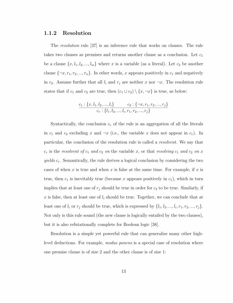
The resolution rule [37] is an inference rule that works on clauses. The rule

takes two clauses as premises and returns another clause as a conclusion. Let c1

be a clause {x, l1, l2, ..., lm} where x is a variable (as a literal). Let c2 be another

clause {¬x, r1, r2, ..., rn}. In other words, x appears positively in c1 and negatively

in c2. Assume further that all li and rj are neither x nor ¬x. The resolution rule

states that if c1 and c2 are true, then (c1 ∪ c2) \ {x,¬x} is true, as below:

c1 : {x, l1, l2, ..., li} c2 : {¬x, r1, r2, ..., rj}cr : {l1, l2, ..., li, r1, r2, ..., rj}

Syntactically, the conclusion cr of the rule is an aggregation of all the literals

in c1 and c2 excluding x and ¬x (i.e., the variable x does not appear in cr). In

particular, the conclusion of the resolution rule is called a resolvent. We say that

cr is the resolvent of c1 and c2 on the variable x, or that resolving c1 and c2 on x

yields cr. Semantically, the rule derives a logical conclusion by considering the two

cases of when x is true and when x is false at the same time. For example, if x is

true, then c1 is inevitably true (because x appears positively in c1), which in turn

implies that at least one of rj should be true in order for c2 to be true. Similarly, if

x is false, then at least one of li should be true. Together, we can conclude that at

least one of li or rj should be true, which is expressed by {l1, l2, ..., li, r1, r2, ..., rj}.

Not only is this rule sound (the new clause is logically entailed by the two clauses),

but it is also refutationally complete for Boolean logic [38].

Resolution is a simple yet powerful rule that can generalize many other high-

level deductions. For example, modus ponens is a special case of resolution where

one premise clause is of size 2 and the other clause is of size 1:

13

{¬p, q} {p}{q}

Removing a literal by unit propagation is another special case, e.g.,:

{¬x, p, q, r} {x}{p, q, r}

Note that a resolvent can be an empty clause (i.e., contradiction or inconsis-

tency). For example,

{¬p} {p}{}

Typical SAT solvers designed for solving real-world SAT problems take and

store an input problem instance in the form of clauses (i.e., as a set of clauses). In

some sense, the architecture of these solvers is simple in that these solvers work

only on clauses. At any point, all information about an input theory is stored

only in terms of clauses in a solver. Such a solver continuously adds, removes,

derives, simplifies, and/or modifies clauses during execution. Typically, every such

operation can be described by a series of resolution applications. Indeed, a broad

class of practical SAT solvers are as powerful as general resolution [23].

For this reason, a typical SAT solver can also be seen as a propositional resolu-

tion proof system from a theoretical perspective. A propositional resolution proof

system is a formal system that proves inconsistency of a propositional theory (i.e.,

refutes a theory) by using only resolution. All assertions in this proof system are

clauses. The proof system continuously derives resolvents until the empty clause

is derived, at which point the proof system has refuted the given theory. The

14

resolution proof system is perhaps the simplest non-trivial proof system [40].

1.2 DP

The Davis-Putnam algorithm (DP) [11] is a decision procedure to determine the

satisfiability of a CNF formula. The paper describing the algorithm was published

in 1960.

Algorithm 1 DP: High-level description

Input: a set of clauses representing a CNF formulaOutput: satisfiability

1: procedure DP(φ)2: if {l} is a unit clause in φ then . Unit rule, optional3: return DP({c \ {¬l} : c ∈ φ, l /∈ c})4:

5: if φ = ∅ then return true . Vacuous truth

6: if ∅ ∈ φ then return false . Empty clause

7:

8: Pick a variable x in φ9: Eliminate x from φ . By resolution

10: return DP(φ)11: end procedure

Algorithm 1 is a high-level description of DP. DP works by iteratively elimi-

nating one variable at a time from an input CNF formula (Line 9). The resulting

formula after the elimination is an equi-satisfiable formula with one fewer variable.

The way DP eliminates a variable is by using resolution (applied in a manner of a

Cartesian product). We describe the exact procedure of variable elimination in no

further detail than what we just described here, as the detailed procedure is not

relevant to our discussion in this thesis. If the empty clause is derived as a resolvent

while eliminating a variable, the input formula is proven to be unsatisfiable. If DP

15

succeeds in eliminating all variables (i.e., the current CNF formula becomes the

empty set of clauses), the formula is proven to be satisfiable (vacuously true). The

original description of DP includes applying the unit rule (Line 2-3) and the pure

rule to simplify a formula. However, such simplifications are for practical efficiency

and thus not strictly required for correctness. For greater simplicity, we did not

include the pure rule in Algorithm 1 (although it is a very simple rule). Moreover,

variable elimination generalizes and subsumes the pure rule. The original DP does

not define how a variable is picked for elimination. Note that DP is not a back-

tracking algorithm. The procedure terminates within n elimination steps where n

is the total number of variables in a formula. However, each elimination step can

generate a large number of resolvents (due to the Cartesian resolution product)

and lead to exponential memory explosion.

1.3 DPLL

The Davis-Putnam-Logemann-Loveland algorithm (DPLL) [12] is a refinement

of the earlier DP algorithm. The paper describing DPLL was published in 1962

(2 years after DP). To address the memory explosion problem of DP, DPLL turns

DP into a backtracking search algorithm; instead of eliminating a variable, DPLL

splits on a variable and solves the two ensuing sub-problems recursively.

Algorithm 2 describes DPLL. Again, for greater simplicity, we do not describe

the pure rule (as we did not describe it in Algorithm 1). (However, it should be

noted that, unlike Algorithm 1, the pure rule is not simulated elsewhere in Algo-

rithm 2. In other words, Algorithm 2 loses one useful deduction facility. However,

the hypothetical deduction power remains unchanged.) Another reason for exclud-

16

Algorithm 2 DPLL: High-level description

Input: a set of clauses representing a CNF formulaOutput: satisfiability

1: procedure DPLL(φ)2: if {l} is a unit clause in φ then . Unit rule3: return DPLL({c \ {¬l} : c ∈ φ, l /∈ c}4:

5: if φ = ∅ then return true . Vacuous truth

6: if ∅ ∈ φ then return false . Empty clause

7:

8: Pick a variable x in φ . Branching heuristic9: return DPLL(φ ∪ {x}) ∨ DPLL(φ ∪ {¬x})

10: end procedure

ing the pure rule besides simplicity is that the pure rule is a relatively expensive

operation in practice; in particular, state-of-the-art solvers do not implement the

pure rule. (However, although rare, there have been recurring efforts to utilize

the pure rule, e.g., [41].) Note that Algorithm 2 is recursive. In practice, DPLL

is implemented as an iterative version for efficiency. Any standard techniques to

convert a recursive algorithm to an iterative version can be used, such as explicitly

managing the recursion stack. However, in practice, an iterative DPLL version

does not explicitly save intermediate equi-satisfiable formulas in a stack for sim-

ulating recursion because these formulas can be very large. Likewise, practical

implementations do not directly modify formulas (e.g., explicitly removing literals

from a clause or removing clauses) but instead make use of partial valuations. In

other words, practical implementations assign truth values to individual variables

while leaving the input formula unchanged at all times. By maintaining a partial

assignment that dynamically changes throughout execution, the input formula can

be evaluated on demand with respect to the current partial assignment.

Algorithm 3 is an example of an iterative version of DPLL. This algorithm

17

Algorithm 3 DPLL: Iterative version

Input: a set of clauses representing a CNF formulaOutput: satisfiability

1: procedure DPLL(φ)2: stack level ← 03: repeat4: status ← BooleanConstraintPropagation()5: if status = CONFLICT then6: if stack level = 0 then return false

7: stack level ← stack level - 18: BacktrackTo(stack level)9: assign true to decision at[stack level] . Flip the last decision

10: else11: if all variables are assigned then return true

12: Pick an unassigned variable x . Branching heuristic13: stack level ← stack level + 114: assign false to x . Try false first15: decision at[stack level] ← x

16: end if17: end procedure

simulates recursion by explicitly storing the current recursion level in a program

variable stack level. We assume that the algorithm stores information associated

with each recursion level in an explicit stack and restores the information properly

when necessary. For example, if a variable x is assigned a value at level 10, we

assume that x becomes unassigned when DPLL backtracks to level 9. decision at is

such a stack that stores which variable was picked for branching at each recursion

level. BooleanConstraintPropagation (BCP) is a procedure that applies the unit

propagation rule until a formula reaches a fixpoint (i.e., no more unit clauses

exist) or a conflict occurs (i.e., the empty clause is derived). Again, iterative

DPLL would not explicitly remove literals from a clause to make the clause unit

or empty but rather maintain a partial assignment. With partial valuation, a

clause is effectively seen as unit (or empty) when the clause is unit (or empty)

18

with respect to a partial assignment. For example, a clause {p, q, r} is considered

unit when q and r are assigned false, because we can actually derive a unit clause

{p} in this case (by applying modus ponens twice). If a conflict occurs after BCP

at the top level 0 (Line 6) (i.e., the empty clause exists while no decision has ever

been made), the formula is unsatisfiable. If a conflict occurs, but not at the top

level, BacktrackTo restores the previous partial assignment at the specified level

by undoing all variable assignments made after that level. Note that Algorithm 3

always backtracks one level, i.e., flips the last decision (Line 9). If BCP completes

with no conflict and all variables are assigned1, the formula is satisfiable (Line 11).

Otherwise, if there remain unassigned variables, DPLL picks one variable among

them as a branching variable. From now on, we will call a branching variable a

decision variable. Similarly, we will call a recursion stack level a decision level.

This DPLL version always tries assigning false first to a decision variable. (For a

number of reasons, assigning false first is a popular strategy [45] in modern solvers,

including MiniSat, Glucose, and their derivatives.)

One advantage of an iterative version of DPLL over a recursive version is the

ability to backtrack multiple levels. Algorithm 4 is a more generalized version with

this ability. Algorithm 4 and Algorithm 3 are identical except for Lines 7-8. We

assume that AnalyzeConflict has the ability to analyze the most recent conflict and

suggest a good backtracking level from the analysis.

1Instead, a solver may check if every clause is satisfied. In fact, by checking clauses insteadof variables, a solver may terminate early with a partial assignment, since a partial assignmentmay satisfy all clauses. However, checking whether every clause is satisfied is very expensive toimplement in practice. Therefore, modern solvers instead check whether all variables in a formulaare fully assigned, as in Algorithm 3.

19

Algorithm 4 DPLL: Generalized iterative version

Input: a set of clauses representing a CNF formulaOutput: satisfiability

1: procedure DPLL(φ)2: stack level ← 03: repeat4: status ← BooleanConstraintPropagation()5: if status = CONFLICT then6: if stack level = 0 then return false

7: bt level ← AnalyzeConflict()8: stack level ← bt level9: BacktrackTo(bt level)

10: assign true to decision at[stack level] . Flip the decision11: else12: if all variables are assigned then return true

13: Pick a variable x . Branching heuristic14: stack level ← stack level + 115: assign false to x . Try false first16: decision at[stack level] ← x

17: end if18: end procedure

1.4 CDCL

DPLL can be extended with Conflict-Driven Clause Learning (CDCL) [4, 5].

CDCL was introduced in the solver GRASP [4, 5] in 1996, more than 30 years after

the advent of DPLL. CDCL has been shown to be very effective on real-world SAT

problems. In fact, almost all modern SAT solvers used in industrial domains are

DPLL solvers extended with CDCL. The power of CDCL comes from the ability

to learn new lemmas (clauses) by analyzing the root cause of a conflict. In fact,

CDCL derives new clauses whenever a conflict occurs. New clauses are logical

consequences of an input theory (formula). In other words, new learned clauses

are redundant and can be discarded freely.

20

Intuitively, CDCL analyzes a conflict and reasons about the root cause of the

conflict. CDCL then gives one or more reasons for the conflict in the form of a

clause. For example, suppose that a conflict occurred when variables x1, x2, . . . x100

are currently all assigned true. Suppose further that CDCL learned a new clause

{¬x10,¬x20,¬x30} after analyzing the conflict. The clause tells us that at least

one of x10, x20, and x30 should have been assigned false. This observation opens

up the possibility of non-chronological backjumping. For example, suppose that

x10, x20, and x30 were assigned at, respectively, decision levels 10, 20, and 30.

Suppose further that the current decision level is 30 (i.e., 30 variables are decision

variables, and the remaining 70 are assigned by BCP). The new learned clause

tells us that x30 should have been assigned false at an earlier decision level than

the current level 30. For example, if we had had this clause from the beginning,

then at level 20, the clause would have been unit and triggered unit propagation.

Therefore, we may now decide to backjump directly to level 20 from the current

decision level 30. Backjumping to level 20 will make the clause unit, and BCP

will immediately set x30 to false. (In fact, the clause becomes unit anywhere from

level 20 to level 29.) In other terms, this clause can assert the value of x30 after

backjumping (to any level between 20 and 29). Every learned clause in modern

solvers has this asserting characteristic (i.e., exactly one literal is assigned at the

current level). For this reason, a learned clause is often called an asserting clause.

In principle, there is no restriction on how many clauses can be learned from

each conflict. In fact, in early versions of CDCL, there existed solvers that learned

several clauses per conflict (e.g., GRASP [4]). However, modern solvers learn only

one asserting clause per conflict [16].

Algorithm 5 describes DPLL extended with CDCL. Often, this extended DPLL

21

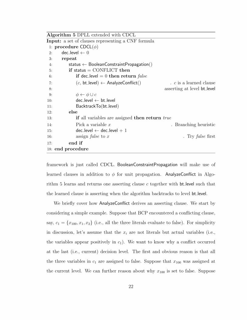
Algorithm 5 DPLL extended with CDCL

Input: a set of clauses representing a CNF formula1: procedure CDCL(φ)2: dec level ← 03: repeat4: status ← BooleanConstraintPropagation()5: if status = CONFLICT then6: if dec level = 0 then return false

7: (c, bt level) ← AnalyzeConflict() . c is a learned clause8: asserting at level bt level9: φ← φ ∪ c

10: dec level ← bt level11: BacktrackTo(bt level)12: else13: if all variables are assigned then return true

14: Pick a variable x . Branching heuristic15: dec level ← dec level + 116: assign false to x . Try false first

17: end if18: end procedure

framework is just called CDCL. BooleanConstraintPropagation will make use of

learned clauses in addition to φ for unit propagation. AnalyzeConflict in Algo-

rithm 5 learns and returns one asserting clause c together with bt level such that

the learned clause is asserting when the algorithm backtracks to level bt level.

We briefly cover how AnalyzeConflict derives an asserting clause. We start by

considering a simple example. Suppose that BCP encountered a conflicting clause,

say, c1 = {x100, x1, x2} (i.e., all the three literals evaluate to false). For simplicity

in discussion, let’s assume that the xi are not literals but actual variables (i.e.,

the variables appear positively in c1). We want to know why a conflict occurred

at the last (i.e., current) decision level. The first and obvious reason is that all

the three variables in c1 are assigned to false. Suppose that x100 was assigned at

the current level. We can further reason about why x100 is set to false. Suppose

22

that x100 was set to false due to unit propagation triggered by another clause

c2 = {¬x100, x888, x999}. That is, x100 had to be assigned false in c2 because the

other two literals x888 and x999 were already false. In other words, setting x888 and

x999 to false will first force x100 to be false, which will in turn falsify c1 because

x1 and x2 are already false. Therefore, to avoid the conflict, x1, x2, x888, and x999

should not be all false at the same time. Then, the following clause concisely

expresses what we just said: cl = {x1, x2, x888, x999}. cl says that at least one of

the four literals should be true. Notice that, at this point, we already learned the

new clause cl after analyzing the conflict. This process of inference to derive cl is

actually an application of the resolution rule. Resolving c1 and c2 on x100 yields

the resolvent cl:

c1 : {x100, x1, x2} c2 : {¬x100, x888, x999}cl : {x1, x2, x888, x999}

The new clause may or may not be asserting. (Recall that a clause is asserting

when only one literal in the clause is assigned at the current decision level.) If cl

is not asserting, we can continue to apply resolution on cl in the same manner as

before until a new resolvent becomes an asserting clause. This entire process is

precisely the clause learning mechanism in CDCL. To summarize, modern CDCL

solvers learn a new asserting clause from a conflict by applying a series of resolution

steps to the conflicting clause. The order in which the resolution steps are applied

is the reverse chronological order of assignments to variables. In other words, we

track back how variables are assigned chronologically. Note that we are guaranteed

to reach an asserting clause when we track back assignments to variables this way.

This is because every assignment to a variable at the current level started with

23

a single assignment to a decision variable. That is, in the worst case, we will

track all the way back to the decision variable. In this worst case, the decision

variable becomes an asserting literal. Therefore, the effect of this worst case is to

flip the last decision, although we may still backtrack multiple levels. However,

we can often reach an asserting clause before reaching a decision variable. Modern

solvers stop at the first encounter of any asserting clause. This scheme of learning

the first asserting clause is called First Unique Implication Point (First-UIP or

1-UIP) learning. (For a formal definition of UIP, see [5].) Learning 1-UIP clauses

is considered to be the best learning scheme [46, 47, 107].

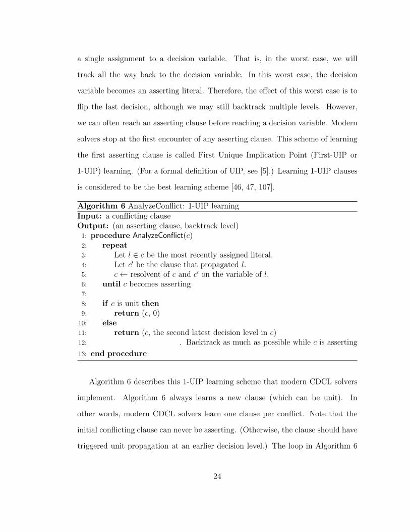
Algorithm 6 AnalyzeConflict: 1-UIP learning

Input: a conflicting clauseOutput: (an asserting clause, backtrack level)

1: procedure AnalyzeConflict(c)2: repeat3: Let l ∈ c be the most recently assigned literal.4: Let c′ be the clause that propagated l.5: c← resolvent of c and c′ on the variable of l.6: until c becomes asserting7:

8: if c is unit then9: return (c, 0)

10: else11: return (c, the second latest decision level in c)12: . Backtrack as much as possible while c is asserting

13: end procedure

Algorithm 6 describes this 1-UIP learning scheme that modern CDCL solvers

implement. Algorithm 6 always learns a new clause (which can be unit). In

other words, modern CDCL solvers learn one clause per conflict. Note that the

initial conflicting clause can never be asserting. (Otherwise, the clause should have

triggered unit propagation at an earlier decision level.) The loop in Algorithm 6

24

will run at least one iteration. In the worse case, the loop runs until an asserting

literal in c is a decision variable, as explained before. In any case, because c is

asserting, the asserting literal in c is the only literal assigned at the current level.

Other literals are assigned at earlier levels. The algorithm returns a backtrack

level that is the second latest level among the decision levels of literals in c. (The

latest level is of course the current level.) In other words, we backtrack as much

as possible while c remains asserting. For example, if {l1, l2, l3, l4} is the learned

clause c, and the literals l1, l2, l3 and l4 are assigned, respectively, at levels 10,

20, 30, and 40 (therefore l4 is an asserting literal and the current decision level

is 40), then the backtrack level is 30. Although it is not incorrect to backtrack

to an earlier level than 30, doing so would unassign two or more literals (i.e., the

clause would no longer be asserting). It is also theoretically possible to backtrack

to a level later than 30, say, to level 35. However, asserting l4 may trigger unit

propagation, which in turn may result in clashes with previous assignments made

between level 31 and 35. It may be possible to reconcile the clashes at level 35.

However, reconciling the clashes would require more effort whereas backtracking to

level 30 completely avoids this complexity. This is one reason that modern solvers

backtrack as much as possible while the learned clause remains asserting.

1.4.1 VSIDS Branching Heuristic

Algorithm 5 does not define how to pick a decision variable for search space

branching. Many heuristics have been proposed, but here we only introduce one

heuristic: the Variable State Independent Decaying Sum (VSIDS) [6]. The VSIDS

heuristic, introduced in the solver zChaff [6], has long been a standard branching

heuristic in CDCL. Besides clause learning, the most important element in CDCL

25

is the VSIDS heuristic [48]. The VSIDS heuristic is considered crucial for achiev-

ing high efficiency on application benchmarks [48]. We actually describe what

some researchers call Exponential VSIDS (EVSIDS) [48, 49, 2], a popular modern

implementation of VSIDS as implemented in MiniSat [2]. Actually, EVSIDS was

originally proposed by the authors of MiniSat. In this thesis, VSIDS always refers

to EVSIDS, as we never reference the original Chaff implementation.

Intuitively, the VSIDS heuristic focuses on solving the current sub-problem

where the solver is working hard to rectify recent conflicts. Basically, when picking

a decision variable, the VSIDS heuristic gives more priority to the variables involved

in recent conflict analyses. Specifically, VSIDS maintains activity scores for each

variable. The idea is to pick the most “active” variable (i.e., the variable with the

highest score) as a decision variable. Informally, variables are considered active

if they actively participated in recent conflict analyses. That is, if a variable x

is observed in AnalyzeConflict (Algorithm 6), the activity score of x is bumped

by a certain amount. (The score is bumped once even if x is observed multiple

times in a single conflict analysis.) However, activity scores are also decayed over

time. If a certain variable was not observed in the most recent conflict analysis,

the activity score of the variable is decreased. Therefore, variables inactive for a

long time keep losing priority in decision variable selection over time. Instead of

actually decreasing activity scores, an actual EVSIDS implementation simulates

this decaying effect by bumping activity scores with higher and higher amounts.

For example, if activity scores were increased by 1 (actual initial bumping amount

in MiniSat) in the current conflict analysis, scores will be increased by 1 × f in

the next conflict analysis where f > 1. In MiniSat and hence many MiniSat-

derivatives, f = 1/0.95. We call 1/f (i.e., 0.95 in MiniSat) the variable decay

26

factor. Note that the bumping amount can overflow eventually, so it is necessary

to rescale all the activity scores from time to time.

1.4.2 Learned Clause Management

Algorithm 5 endlessly learns and adds new clauses to the current set of clauses.

In practice, the speed of learning new clauses can be very fast. Modern SAT solvers

routinely generate thousands of clauses per second [14, 26]. Depending on the

problem instance, solvers may even generate a few tens of thousands of clauses per

second. Therefore, adding clauses without ever removing some is problematic due

to high memory consumption. Even if all learned clauses can be fit into physical

memory before termination, maintaining a huge set of clauses causes inefficiency

in various places. For these reasons, solvers have a mechanism to manage learned

clauses.

Very early solvers employed a crude strategy of periodically forgetting learned

clauses according to some criteria. The rationale for employing such a strategy

was mostly from the perspective of having some way to address the memory explo-

sion problem [16, 60, 2, 6]. It is relatively recent that learned clause management

became an active topic of research [16]. It was the solver Glucose [3] which first

emphasized that the management of the clause database is an essential ingredi-

ent [3, 52] to the solver performance. Glucose has pioneered the research in this

topic to date, bringing continued innovations. Prior to the 2009 version of Glucose,

clause deletion policies in solvers were primarily based on the VSIDS activity of

the clauses [14, 78] as implemented in MiniSat [2]. Nevertheless, from early solvers

to modern solvers (including Glucose), the fundamental way of managing learned

clauses is to periodically prune the learned clause database. At certain periodic

27

intervals, solvers shrink (typically halve) the learned clause database by removing

clauses that seem least relevant or useful. The intervals are usually measured in

terms of the number of conflicts. The number of conflicts is a natural choice be-

cause CDCL learns one clause per conflict. In other words, using an interval of n

conflicts ensures that a reduction will happen after learning n clauses.

Most solvers gradually increase the intervals between database reductions. In-

creasing intervals ensures the completeness (i.e., guaranteed termination with a

definite answer) of a solver. Note that AnalyzeConflict (Algorithm 6) always re-

turns a new clause that does not currently exist in the solver’s clause database.

If the clause already existed, then that clause would have asserted its asserting

literal at an earlier decision level. In other words, the current conflict would have

been avoided earlier. Note that there can exist only a finite number of clauses for

a finite number of variables. Therefore, if a solver is given enough time, solvers

can exhaust all clauses by learning. Gradually increasing intervals eventually gives

a solver enough time to learn all possible clauses. From these arguments, we can

conclude that the solver will eventually terminate. Interestingly, although com-

pleteness is meaningless in the presence of a timeout during execution in practice,

almost all solvers gradually increase database reduction intervals. For example,

in SAT Competition 2014 [106], among a few tens of participating solvers exclud-

ing our solvers, the only CDCL solver that did not have increasing intervals was

ROKK [91], to the best of our knowledge. (As such, our solvers that we intro-

duce in later chapters are atypical in that they give up completeness.) Similarly,

in SAT-Race 2015 [105], all participating solvers retained completeness by having

increasing reduction intervals, with the exception of our solvers and a couple other

solvers that adopted our strategy. This observation suggests that solvers do not

28

increase intervals just for completeness. Rather, the intention of increasing the

intervals is that it aids the gradual accumulation of more and more useful learned

clauses by not setting a hard limit.

In the following, we describe the two strategies of managing learned clause

implemented in MiniSat and Glucose.

1.4.2.1 MiniSat Strategy

The latest release of MiniSat predates Glucose. As mentioned before, Glucose

has brought significant attention to the research on learned clause management.

Relatively, not much effort had been spent on the aspect of clause management

before the advent of Glucose. For this reason, the management strategy in MiniSat

falls far behind the current state of the art.

Reduction intervals. MiniSat uses, basically, geometric progression for the

gradually increasing intervals. (However, precisely speaking, the intervals are not

for database reduction but for setting the maximum size to which the database

can grow.) Roughly speaking, the size of the clause database is capped to follow

geometric progression. The base of the progression depends on the size of the input

formula. If a formula is large, the base is large. That is, MiniSat allows a bigger

clause database for a larger formula. For this reason, MiniSat sometimes does not

perform any database reduction for large problem instances [51]. It is generally

accepted that MiniSat maintains a relatively huge clause database compared to

modern solvers that employ aggressive database reduction [3].

Clause prioritization. MiniSat uses “activity” of clauses to decide which

clauses to remove or retain. At each database reduction, MiniSat removes roughly

the half of the learned clauses that are deemed least active. This activity-based

29

prioritization is inspired by the great efficiency of the VSIDS branching heuris-

tic [2]. In fact, the activity scores of clauses are computed in the same manner as

VSIDS. If a clause is used in resolution in the conflict analysis (Algorithm 6), the

activity score of the clause is bumped. Just like in VSIDS, activity scores of clauses

are decayed. As such, this activity-based prioritization has a dynamic nature. It

has been shown that this activity-based prioritization outperforms the size-based

prioritization (where short clauses survive) [68].

1.4.2.2 Glucose Strategy

Reduction intervals. In Glucose, the intervals between database reductions

follow an arithmetic progression (with some minor adjustments). For the most

recent versions of Glucose, the intervals (in terms of conflicts) are the following

series (plus or minus some minor adjustments): 2000, 4600, 7200, 9800, 12400, . . . 2

Compared to MiniSat, these intervals in Glucose result in a much more aggressive

database reduction, and hence a very compact database. In fact, Glucose has

evolved to employ more and more aggressive database reduction strategies.

Clause prioritization. Glucose proposed a metric called Literal Block Dis-

tance (LBD) [3] to predict the usefulness or relevance of clauses. LBD is defined to

be the number of different decision levels in a clause, assuming that every literal

in the clause is assigned. For example, given a clause {l1, l2, . . . , l100}, if l10, l15, l23

are assigned at decision level 3 and the rest of the literals are assigned at decision

level 95, then the LBD of the clause is 2 with this variable assignment. Note that

a long clause may have a low LBD as in this example. At each database reduction,

2It is often misunderstood that the intervals are 2000+300x (e.g., in [58]) because the authorsof Glucose mistakenly reported a wrong multiplicative factor of 300 on several occasions [54, 55,56, 57]. Precise calculation gives the intervals of 2000 + 2600x.

30

Glucose removes roughly the half of learned clauses that have the highest LBD.

LBD quickly became the norm and is now recognized as one of the standards in

CDCL [16]. The LBD metric is largely static compared to the activity metric of

MiniSat. Glucose computes and assigns the LBD value to a new clause at the time

the solver learns the clause. Glucose does have a feature to dynamically update

LBD values of existing clauses. However, updating the LBD of a clause happens

only when the clause is used in conflict analysis. Moreover, the LBD value is only

updated if the value can be lowered.

1.4.3 Restarts

From time to time during search, contemporary CDCL solvers backtrack to

the top decision level 0. Backtracking to level 0 means abandoning the current

search branch and restarting a new search. This backtracking can happen at

an arbitrary point of search. This level-0 backtracking is conventionally called

a restart. Implementation-wise, restarting is nothing more than backtracking to

level 0. Although restarts are not a sophisticated technique, there is mounting

evidence that this technique has a crucial impact on performance [53]. Note that,

regardless of the frequency of restarts, restarts do not compromise the completeness

of a typical solver. As long as there is a guarantee that conflicts keep occurring

in the presence of restarts, solvers will continuously learn new clauses and exhaust

all possible clauses eventually.

Restarts were initially proposed by Gomes et al. (1998) [19] to eliminate the

(empirically observed) heavy-tailed phenomenon of DPLL-like backtracking algo-

rithms [19]. The heavy-tailed phenomenon is characterized by a non-negligible

probability of hitting a problem that requires exponentially more time to solve

31

than any problem that has been encountered before [20]. In simple terms, an un-

lucky solver using a certain random seed may take exponentially more time than

the same solver using another random seed when solving the same problem. In

this argument, randomized restarts can reduce the variance in solving time that is

observed when running solvers multiple times with different random seeds. There-

fore, the argument for the success of restarts given by Gomes et al. is only relevant

for solvers with a certain level of randomness [53]. However, modern solvers often

make no use of randomness at all (e.g., MiniSat and Glucose). In fact, there of-

ten exist more recent perspectives that the arguments given by Gomes et al. are

insufficient to explain well the great efficiency of restarts in modern solvers (e.g.

[29, 53]).

Polarity saving [51] (equivalently, polarity caching or phase saving) is often

argued to be crucial for the efficiency of restarts in modern solvers [29, 3]. Almost

all modern CDCL solvers implement polarity saving [48]. Polarity saving is a

simple technique to use the same last-used polarity of a variable when making

a branching decision. For example, suppose that x was assigned true (e.g., by

decision or BCP) at some point and becomes unassigned at a later point. If a

branching heuristic picks x for the next decision variable, the heuristic sets x to true

again by the polarity saving policy. Pipatsrisawat and Darwiche [51] observed that

restarts and backjumps might lead to repetitive solving of the same sub-formulas.

Based on this observation, the paper proposed polarity saving to prevent solvers

from solving the same satisfiable sub-formulas several times. Solvers have evolved

to employ more and more rapid restarts [101, 1, 102, 103], so polarity saving is

particularly crucial in modern solvers [29, 1]. For this reason, polarity saving is a

de facto standard in current CDCL solvers.

32

Various policies for when to make a restart have been proposed. Some of the

early solvers used a very simple policy to restart at a fixed interval of every x

conflicts (e.g., x = 16000 in Siege [42], x = 2000 in Eureka [61], x = 700 in

zChaff 2004 [6], and x = 500 in Berkmin [60]) [53]. Walsh [59] suggested to use

a geometric series for the restart intervals between conflicts. MiniSat 1.13 was

the first to demonstrate the effectiveness of the geometric restart strategy. For

example, the restart intervals of MiniSat 2007 adhered to the following geometric

series: 100, 150, 225, . . . (i.e., 100 × 1.5i−1 where i is the i-th interval). PicoSAT

2008 [62] nested a geometric series inside another geometric series for the intervals.

In this strategy, the inner geometric series runs only for a finite iterations over and

over, but the number of iterations follow another geometric series. As a result,

the restart intervals of this inner-outer strategy grow much slower than a single

geometric series. Another strategy based on the Luby series [50] was also suggested.

The Luby series is characterized by the following pattern: 1, 1, 2, 1, 1, 2, 4, 1,

1, 2, 1, 1, 2, 4, 8, 1, . . . . For example, the restart intervals in RSat 2.0 [66] and

TiniSat [67] are the Luby series where each number in the series is multiplied by

512 (i.e., 512, 512, 1024, 512, 512, 1024, 2048, . . . ). Recent versions of MiniSat

(2.1 and 2.2) and PrecoSAT [63] multiplied 100 to each number in the Luby series

(i.e., 100, 100, 200, 100, 100, 200, 400, . . . ) [1]. Whenever we mention the Luby

restart strategy, we specifically refer to the previous intervals as implemented in

MiniSat (i.e., the Luby series multiplied by 100).

1.4.3.1 Luby Restarts

The Luby series deserves more explanation as the Luby-series restart strategy

is one of the subjects in Chapter 3. Formally, the Luby series is defined recursively

33

as follows, where ai is the i-th number in the series:

ai =

2k−1 if ∃k ∈ N. i = 2k − 1

ai−2k−1+1 if ∃k ∈ N. 2k−1 ≤ i < 2k − 1

This is a well-defined series as the two conditions are mutually exclusive. The

series is known to have some nice theoretical characteristics, e.g., to be log optimal

when the runtime distribution of a problem is unknown [50]. Experiments have

also shown that the Luby series outperforms the other restart strategies mentioned

above [64, 53]. However, it is not clear what the reason is that the Luby series

works well in practice. The relevance of such nice theoretical results about Luby to

DPLL has only been empirical. Nevertheless, because of the empirical superiority

of the Luby strategy to other restart strategies, the Luby series has been the restart

method of choice in several state-of-the-art solvers in the past [29, 101, 1]. Par-

ticularly, the adoption of Luby in MiniSat and the impressive performance of the

solver made Luby the default restart strategy in many MiniSat-derivatives. Solvers

using the Luby strategy generally exhibit frequent restarts [111, 1]. (However, the

Luby strategy is not deemed frequent from today’s perspective [29].)

The restart strategies introduced so far (except for randomized restarts) have a

static nature: the restart intervals are pre-determined and thus independent of the

program state in a running solver. Policies with dynamic elements have also been

tested or implemented successfully [49, 62, 63, 29, 65, 53]. Some of the dynamic

strategies have a static restart strategy as a basis and adjust the frequency of the

underlying restarts dynamically (e.g., skip, induce, or suppress restarts). Some

other strategies do not even base themselves on a uniform strategy. Dynamic

restart strategies have received much attention recently as more and more recent

34

solvers adopt dynamic restart strategies to improve performance.

1.4.3.2 Glucose Restarts

One of the most successful dynamic strategies is the LBD-based restart strategy

introduced in Glucose [29]. We determined that the top 23 solvers (including

Lingeling 2015 [72]) that participated in the main sequential track of SAT-Race

2015 used the Glucose restart strategy or a minor variant. The majority of the

23 solvers used the Glucose strategy as the only and primary restart strategy by

default. (In fact, many of the solvers are either directly based on Glucose or use

Glucose as a sub-component in an off-the-shelf manner.) Even the minority of

the remaining competing solvers still use the Glucose strategy or its variants for a

significant portion of their execution. From these observations, we can recognize

that the Glucose restart strategy is close to being considered a current standard in

CDCL. (However, we emphasize that, as demonstrated particularly by Lingeling

2014 [73] and 2013 [74], other dynamic strategies such as agility- and/or saturation-

based restarts [49, 73] can also be very competitive.)

Intuitively, the Glucose restart strategy is designed to escape from a situation

where the solver is learning high-LBD clauses. Specifically, the Glucose strategy

triggers a restart if the solver seems to be learning clauses with higher LBD values

than the global LBD average. The global LBD average is simply an average of

LBD values of all the past learned clauses. Before branching on a variable, Glucose

compares the global LBD average against the local LBD average of the most recent

50 clauses. Glucose triggers a restart if the local average multiplied by 0.8 is

greater than the global average. (The multiplicative factor 0.8 gives some margin

for the local average to exceed the global average.) However, right after a restart,

35

Glucose suppresses restarts for the next 50 conflicts before another restart can

happen. In other words, at least 50 conflicts should occur before the next restart

can be triggered. Compared to the Luby strategy (as implemented in MiniSat),

this restart strategy generally results in much more rapid restarts [29]. On some

SAT problem instances, this strategy can trigger restarts every 50 conflicts [29].

The authors of Glucose soon identified one particular problem with these rapid

restarts. For example, if restarts are triggered every 50 conflicts, the solver cannot

find a solution (for satisfiable SAT problems) if the solver is unable to make a full

variable assignment before conflicts occur 50 times.

To address the problem of too rapid restarts, later versions of Glucose intro-

duced a small enhancement to block restarts in certain situations [29]. If a certain

condition is met, this enhancement prevents restarts from happening for the next

50 conflicts. Intuitively, Glucose blocks restarts if the solver seems to be approach-

ing a full variable assignment. More precisely, the solver checks if a lot of variables

are suddenly and unusually assigned. Implementation-wise, the solver checks if

the number of currently assigned variables exceeds the average number of assigned

variables for the past 5000 conflicts multiplied by 1.4. That is, Glucose blocks

restarts if variables are currently at least 1.4 times more assigned than the aver-

age. As long as the said condition is met, Glucose keeps blocking restarts (e.g.,

restarts can be blocked for a long time). Finally, as an optimization, Glucose does

not block restarts for the first 10,000 conflicts.

36

1.5 Machine Configurations

In this thesis, we use the following three machine configurations for evaluating

solver performance.

1. Machine configuration A. The StarExec cluster [75]. We used the nodes

with the following machine specs: Intel Xeon CPU E5-2609 @ 2.40GHz and

256GB RAM. We always set 8GB for the memory limit for each process.

2. Machine configuration B. Intel Core i5-4460S @ 2.90GHz and 12GB RAM

running Linux.

3. Machine configuration C. Intel Core 2 Duo E8400 @ 3.00GHz and 4G

RAM running Linux.

37

Chapter 2

Learned Clauses and Industrial

SAT Problems

The introduction of Conflict-Driven Clause Learning (CDCL) was a revolution-

ary moment: DPLL solvers extended with CDCL were several orders of magnitude

faster than the decade-old plain DPLL. Learning clauses through conflicts imme-

diately enabled building very efficient and practical SAT solvers, manifesting the

potential and viability of using SAT for real-world applications in numerous indus-

trial domains. Since the advent of CDCL, we have witnessed dramatic progress

in SAT research, with conflict clause learning as the starting point and basis for

continued innovations [42, 2]. It has been shown that conflict clause learning is the

technique that has the greatest relative importance for solver performance com-

pared to other major features of CDCL solvers by a large margin [76]. Also, from a

theoretical point of view, learning and knowing more lemmas brings many benefits.

As such, it is normally believed that accumulating more and more clauses learned

through conflict clause learning is crucial for solver performance.

38

In this chapter, we present a largely unconventional view that learned clauses

play a surprisingly insignificant role in CDCL, from the perspective of actual per-

formance and the capability to solve real-world problems. Our view does not

conflict with the fact that learning (and hence its side-effects such as effects on

the VSIDS branching heuristic, non-chronological backtracking, etc) is the most

important feature that accounts for the great efficiency of CDCL SAT solvers. It

is crucial to understand that keeping and managing learned clauses is an entirely

different story from learning itself. In fact, it is well known empirically that keep-

ing too many clauses is detrimental to solver performance [3, 52, 78]. If a clause

database grows too large, it may even paralyze a solver completely. We will go

far beyond this view and show that only a small fraction of learned clauses hav-

ing very high quality (measured by a certain metric) is meaningful to retain in a

solver in an ultimate sense. By the ultimate sense, we mean that we are able to

solve more problems faster, despite some possible disadvantages. Particularly, it

will be very surprising to see that learned clauses are strikingly unimportant for

finding a model for satisfiable problem instances. Also for unsatisfiable instances,

we will show that most of the real-world problems that modern solvers can tackle

efficiently have a near-constant maximum width1 (in terms of clause size and/or

LBD) for the great portion of their resolution proof tree.

To summarize, we show in this chapter that learned clauses in CDCL play a

surprisingly insignificant role in solving a problem efficiently. We first test a hy-

pothesis that most of the unsatisfiable real-world problems that CDCL solvers can

tackle efficiently have an “easy and short” proof of unsatisfiability. We test the

1In a formal context, the width of a resolution proof is defined to be the maximal size of anyclause in the proof [40]. Here, we extend the notion to include the LBD of any clause in additionto the size.

39

hypothesis by severely limiting the practical capability of a CDCL solver so that

the solver is forced to use “easy and short” lemmas for deduction for the significant

portion of its proof of unsatisfiability. The experimental results will also confirm

that learned clauses are even less important for satisfiable problems. More surpris-

ingly, we shall see that a solver with limited capabilities can often outperform its

unrestricted counterpart on both satisfiable and unsatisfiable problems. We show

from these results that the current state of CDCL solvers have a limitation in that

they are largely incapable of deriving sophisticated proofs. Finally, by exploiting

these empirical characteristics of CDCL, we propose simple yet effective changes to

the traditional clause management scheme that will improve CDCL performance.

2.1 Learned Clause Management

CDCL SAT solvers must potentially maintain a huge number of learned clauses.

This is especially true for modern solvers where the rates of Boolean Constraint

Propagation (BCP) and conflict analysis are very high. Typically, modern SAT

solvers generate one asserting clause through conflict analysis whenever a conflict

arises. In practice, learned clauses generated in this manner usually make the

clause database grow at an alarming rate. Very early CDCL solvers employed a

crude strategy of periodically truncating the database. The rationale for employ-

ing such a strategy was mostly that of having some way to address the memory

explosion problem [16, 60, 2, 6]. It soon became clear that a fast-growing database

of clauses can cause BCP performance to deteriorate quickly, severely limiting the

capability of a solver. Efforts have been put into prioritizing which clauses to re-

tain or remove. However, relatively modern solvers before the advent of Glucose

40

still had a reluctance2 to remove clauses and thus maintained a huge database in

general. As an extreme example, the last MiniSat version sometimes never removes

learned clauses [51], especially when an input problem is large. It is relatively re-

cent that learned clause management became an active topic of research [16]. It

was Glucose which first pointed out that the management of the clause database

is an essential ingredient [3, 52] to the solver performance. Glucose has pioneered

the research in this topic to date, bringing continued innovations.

Still, even with the recent advances in this topic, the fundamental strategy for

managing a huge number of learned clauses in SAT solvers is to periodically re-

duce the learned clauses database. More elaborate schemes exist, but essentially,

this periodic clause removal is the underlying framework for clause management in

virtually all modern solvers. Typically, solvers halve the database, adding a small

degree of dynamic adjustment at best. While fixing the reduction ratio to 1/2 to

halve the database, solvers contain the rate of database expansion by controlling

the intervals between database reductions. Normally, the intervals between reduc-

tions increases over time by following, e.g., a geometric or arithmetic progression.

This gradual increase of intervals ensures eventual exhaustion of clauses and thus

guarantees completeness (i.e., termination) of a solver. The following lists some of

the goals that we try to achieve with periodic database reduction:

1. We want to accumulate more and more clauses, since learning and knowing

more lemmas is advantageous for diverse reasons.

2. However, we need to periodically forget some that seem less helpful, since

keeping too many clauses severely penalizes BCP efficiency.

2From today’s perspective. In the past, for example, MiniSat was recognized to have anaggressive clause deletion strategy relative to the earlier generation of solvers [77].

41

3. Finally, we need to make the database grow over time, e.g., to prevent repeat-

ing the same conflicts [60, 51] and/or to achieve theoretical completeness.

Each of the above goals is based on some commonly held assumptions about

learned clauses. At the root of such assumptions is often the view that learned

clauses in CDCL are the most important asset we learn during solving. It is

not surprising that there existed a portfolio-based parallel solver in which one

of the portfolio configurations keeps learned clauses as much as possible (until

memory gets low) [79]. For another example, a recent work in 2015 proposes

adding certain kinds of learned clauses to the original formula before starting

the actual solving [16]. Those learned clauses are actually learned by running a

solver as a preprocessor on some sub-problems. Likewise, many researchers believe

that keeping learned clauses is essential to avoid repetition or to ensure making

progress [60, 51]. Some believe that it would always help if we could predict and

keep clauses that will be used frequently in future propagations or conflicts. Even

though we lack clear understanding about the roles of learned clauses in CDCL

at this stage, most of these assumptions seem too obvious not to accept. In this

chapter, we will come to see that some of these assumptions do not hold up under

scrutiny and thus do not justify much consideration in practice.

Nevertheless, we need to understand that there can exist different criteria for

prioritizing which clauses to retain or remove during periodic database reduction.

Prior to Glucose, the criterion was primarily the clause activity [14, 78], i.e., pri-

oritization based on how actively clauses participated in recent conflict analyses.

This activity-based criterion is inspired by the success of the VSIDS branching

heuristic [78]. In fact, the activity scores of clauses are computed in the same way

the VSIDS scores for variables are computed. MiniSat is an exemplary solver using

42

this criterion, and Glucose also makes use of it as a last resort. Work on VSIDS

shows that VSIDS exhibits and exploits locality in search space exploration [80].

It is not hard to imagine that such locality exists, since VSIDS tries to focus on

the current sub-problem by its nature. Because of the same mechanism, we believe

that prioritizing clauses based on activity would similarly exhibit locality; in other

words, it is our conjecture that activity-based prioritization may not be the best

strategy for retaining clauses in terms of long-term usefulness of clauses. Glucose

later introduced and used LBD [3] for prioritizing clauses. LBD has been shown in

many extensive experiments to be a more accurate and effective metric for predict-

ing the quality or usefulness of clauses. LBD quickly became the norm and is now

recognized as one of the standard techniques in CDCL [16]. Almost every state-of-

the-art solver either derives directly from Glucose, implements/adopts Glucose’s

clause management strategy, or utilizes LBD as a core determining factor for many

critical components. It is interesting to note that the initial paper [3] that pro-

posed LBD presented the perspective that LBD is more suited for predicting future

usefulness of clauses than the activity-based prioritization. The paper also stated

that the activity-based criterion is not a guarantee of future significance of clauses

and this is why solvers (such as MiniSat) often let the size of a clause database

grow exponentially [3]. Fundamentally, we agree on this perspective that LBD is

superior to the clause activity in terms of predicting global usefulness. By using

LBD, Glucose can employ an aggressive clause removal strategy and maintain a

compact database [3]. Over time, Glucose has evolved to have increasingly ag-

gressive reduction with huge success [57]. Heavily influenced by Glucose, today’s

solvers maintain a very compact database compared to the solvers before Glucose.

Still, modern solvers take the very basic form of periodically halving the clause

43

database. Solvers sort the entire list of learned clauses by some criteria and trun-

cate the list by half, where the main criterion is usually the LBD. The intervals

between periodic reductions basically follow, e.g., an arithmetic progression so that

the database grows over time, ensuring completeness. This basic form implies that

the state of the art is far from precisely identifying a relevant set of clauses nec-

essary to solve a problem. In this chapter, we propose a more elaborate scheme

designed with a clear intent that deviates from this basic form. The new scheme

is designed in a very specific way rather than empirically derived by many trial-

and-error experiments. This was possible as we gained new insights about which

clauses are really necessary to solve real-world problems in practical settings.

2.2 Low-LBD Learned Clauses

The evolution of Glucose has progressed toward increased aggressiveness in

database reduction. Newer versions of Glucose came with improved performance

while shortening the intervals between reductions to have a more compact database.

The reason for the improvement with more aggressive reduction could be multi-

fold: it might be the increased BCP speed owing to the small number of clauses

to watch; small memory usage hence less system overhead and increased cache

utilization; decreased search space pollution being caused by bad or toxic clauses;

a virtuous cycle in which good clauses can more likely be generated out of good

clauses; long-term side-effects to how search is driven when having more good

clauses and fewer bad clauses; or sophisticated interactions between various com-

ponents in CDCL when working on a small database. Whatever the reason is,

Glucose is already hinting that removing more and more clauses could actually

44

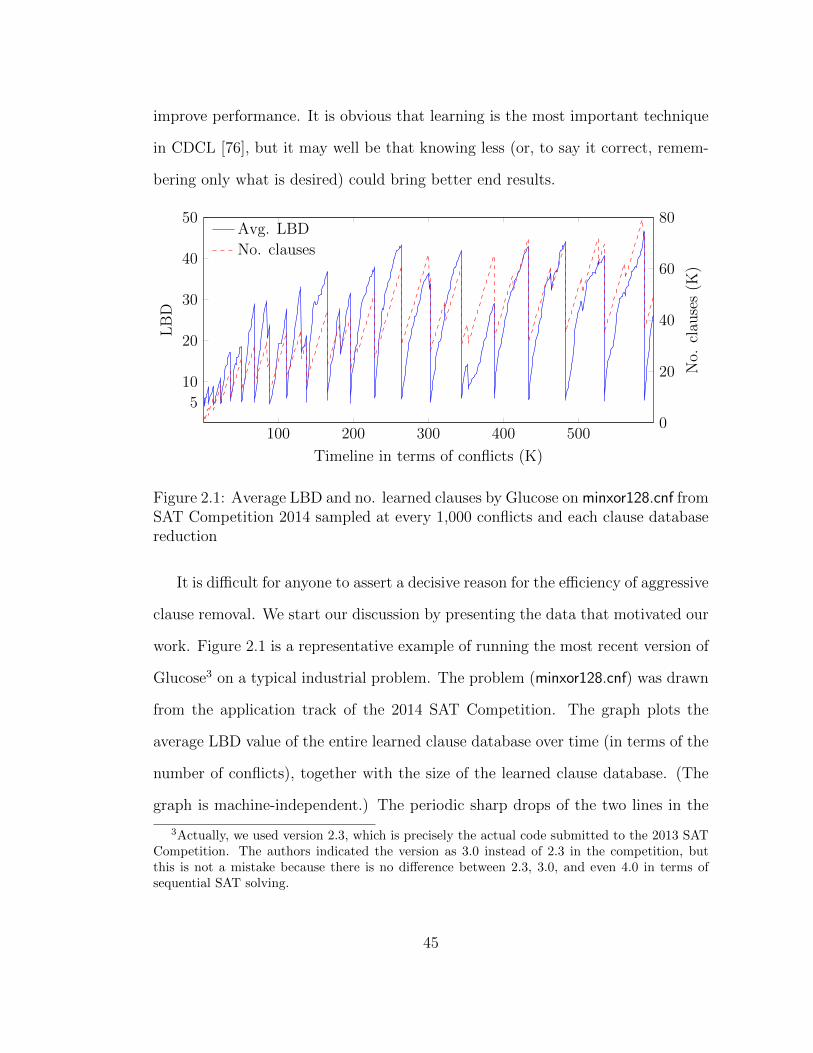
improve performance. It is obvious that learning is the most important technique

in CDCL [76], but it may well be that knowing less (or, to say it correct, remem-

bering only what is desired) could bring better end results.

100 200 300 400 500

5

10

20

30

40

50

Timeline in terms of conflicts (K)

LB

D

Avg. LBD

0

20

40

60

80

No.

clau

ses

(K)

No. clauses

Figure 2.1: Average LBD and no. learned clauses by Glucose on minxor128.cnf fromSAT Competition 2014 sampled at every 1,000 conflicts and each clause databasereduction

It is difficult for anyone to assert a decisive reason for the efficiency of aggressive

clause removal. We start our discussion by presenting the data that motivated our

work. Figure 2.1 is a representative example of running the most recent version of

Glucose3 on a typical industrial problem. The problem (minxor128.cnf) was drawn

from the application track of the 2014 SAT Competition. The graph plots the

average LBD value of the entire learned clause database over time (in terms of the

number of conflicts), together with the size of the learned clause database. (The

graph is machine-independent.) The periodic sharp drops of the two lines in the

3Actually, we used version 2.3, which is precisely the actual code submitted to the 2013 SATCompetition. The authors indicated the version as 3.0 instead of 2.3 in the competition, butthis is not a mistake because there is no difference between 2.3, 3.0, and even 4.0 in terms ofsequential SAT solving.

45

graph indicate that database reductions happen at those points. It is clear that

the average increases locally and globally. What is very interesting is that the

LBD average right after each reduction always drops sharply from a substantially

high value to about 5. Considering that Glucose halves its clause database, we can

infer that the LBD distribution of the entire learned clause database just before a

reduction is very skewed. One half is comprised of clauses with small LBD values

averaging out to around 5. The other half has to have clauses with much higher

LBD values, especially when considering that the average of the first half is about

5. In other words, clauses are learned with very high LBD values most of the

time; the fraction of low-LBD clauses learned is very small. One thing to further

consider about Glucose when interpreting the graph is that once a learned clause

has attained a sufficiently low LBD, the clause has a high tendency to remain in the

database in a stable manner, often forever if the LBD is sufficiently low. The lower

the LBD of a clause is, the higher its chance of being fixed in the database. One

factor that reinforces this tendency is that low-LBD clauses are far more likely to

be involved in BCP and hence conflict analysis too. For clauses involved in conflict

analysis, Glucose dynamically updates the LBD value if it can be decreased (i.e.,

LBD values are never increasing).

With these observations, we hypothesized the reason for the efficiency of Glu-

cose to be the following (which, of course, is only a partial explanation emphasizing

one aspect). By aggressively cleaning learned clauses, Glucose is successful at 1)

collecting only those clauses with very low LBD that have relatively low chances to

be learned; 2) retaining those critically-low-LBD clauses in a stable manner; while

3) frequently removing all the rest and majority of other clauses that are largely

useless. This tendency to keep only such low-LBD clauses is always reinforced

46

with increased aggressiveness in clause removal, although too much aggressiveness

may adversely remove many low-LBD clauses. From our perspective, the current

configuration of Glucose is highly optimized and is very good at striking the right

balance to accumulate more and more critically-low-LBD clauses while constantly

truncating a large body of other useless clauses by aggressive reduction.

With the above observation and considering the continued performance im-

provements brought by the aggressive clause removal in Glucose, we conceived the

following possibility: fundamentally, it is only the low-LBD clauses that actually

contribute to efficient solving of real-world SAT problems. In other words, it may

be that the global usefulness of clauses is severely limited unless their LBD is crit-

ically low. Then, we may still be able to solve many problems efficiently even if we

ignore the majority of learned clauses whose LBD is higher than a certain small

limit. We will show shortly that this is in fact true for real-world problems in

general. Particularly, we will see in Chapter 3 that learned clauses are surprisingly

unimportant for the purpose of finding a solution for satisfiable formulas.

2.3 Evaluation and Discussion

We conducted an experiment to verify our hypothesis that what practically

matters to solve a real-world problem is to accumulate only those clauses with very

small LBD values. We will show shortly that our hypothesis is firmly supported by

the results, at least given the current state of CDCL. This will additionally reveal

some limitations of the state of the art of CDCL.

47

2.3.1 Core and Local Learned Clauses

Taking Glucose as a base solver, we slightly modified it in the following ways:

for some given limit on LBD, the solver accumulates only those learned clauses

whose LBD does not exceed the LBD limit. Precisely speaking, if the LBD of a

learned clause is less than or equal to the given LBD limit, the clause is added to

the clause database permanently. What is unconventional in the context of clause

management is that such clauses are never removed (unless they become trivially

satisfied by top-level facts). We shall call these clauses core learned clauses. On

the other hand, all other clauses whose LBD exceeds the given limit are meant

to be maintained locally and temporarily only. We shall call them local learned

clauses. We make the solver maintain only a small number of local clauses by

setting a hard limit on the total number. Technically, whenever the number of

local clauses reaches 20,000, we throw away half of them. Note that modern SAT

solvers routinely generate thousands of clauses per second [14, 26] (sometimes even

more than 30,000 per second on fast machines depending on problems). In this

sense, this hard limit of 20,000 local clauses is very low and also unconventional.

It is not hard to see that only a small portion of clauses survive as core clauses

while a lot of clauses are learned but removed very quickly. This may raise the

concern that the solver may suffer from repetitive learning. However, as we will

see later, repetitive learning is either not happening or negligible after all. For

prioritizing which local clauses to retain or remove, we decided to use the exact

same criterion of MiniSat: sorting clauses according to the clause activity. Note

that, although LBD is a mostly static measure, recent versions of Glucose have

a feature to dynamically update LBD (although always decreasing) as mentioned

before. As such, if the LBD of a local clause becomes less than the given LBD

48

limit, we promote the clause to a core clause and thus keep it forever. However, we

did not fix the bug from the original Glucose where the dynamic LBD computation

does not exclude the top level (decision level 0). As a consequence, for example, an

LBD value that should have been 3 may be computed to be 4 (i.e., can be larger by

1) for clauses containing level-0 literals. Therefore, in this case, if we set the LBD

limit for core clauses to 3, we will classify the clause as a local clause even though

the clause is a core clause in actuality. Nevertheless, the bug itself does not change

the overall outcome of the experiment or the general conclusion derived from the

outcome. We make a note of this bug here because the LBD values that we use in

the experiment are very low, in the range between 0 and 10. In fact, considering

the bug when interpreting the experimental result actually fortifies our conclusion.

For example, using an LBD limit of 1 in the experiment is effectively equivalent to

using an LBD limit of 0 for clauses containing level-0 literals.

The intuition behind the notions of core and local in this experiment is as

follows. Even though the LBD limit to be qualified as core is deemed too low

from the traditional point of view, we hope that such core clauses collectively

form a sufficiently rich foundation of usable lemmas (clauses). Viewing the CDCL

algorithm as a proof system, we hope that a solver can efficiently derive a proof

of unsatisfiability from the said foundation of core clauses. Here, one underlying

assumption is that LBD is currently the best metric for quantifying the global

usefulness of clauses in the context of constructing a final resolution proof tree.

Moreover, by forcing a small LBD limit, we assume that there usually exists an

“easy and short” proof for (unsatisfiable) real-world problems, i.e., a proof that

can be easily constructed only using low-LBD clauses.

For local clauses, the decision to use the activity-based clause prioritization

49

may seem atypical at first; it has been shown that the LBD is a more accurate

measurement than the clause activity for clause usefulness [78, 3]. Almost all

modern solvers use LBD as a primary criterion [16], and the clause activity is

only secondary at best. However, the activity-based prioritization is a proven and

working strategy based on VSIDS at least. Our assumption is that, although the

clause activity may not be a good metric for quantifying the global usefulness of

clauses, it may be more suitable for capturing the local usefulness. In this sense,

local clauses are maintained mainly for the purpose of properly driving search by

conflicts. This is why we maintain only a small number of local clauses by setting a

hard limit on the total number. Still, the focus of our setup is on the ultimate goal

to accumulate the low-LBD clauses, from which solvers would be able to derive an

easy refutation proof.

One final note is that, theoretically, this clause management scheme makes a

solver incomplete (i.e., no guarantee of termination). However, this does not have

meaningful implications in practice, because, as we will see later, the end result is

that we often become able to solve more problems in less time.

2.3.2 Experimental Results

The core LBD limits that we test in the following experiment range from 0

to 10. The LBD value of 0 means that the solver will not ever have any core

clauses (i.e., only maintaining up to 20,000 local clauses). Note also that solvers

can never learn a clause with LBD 1 from conflicts; when learning a clause, the

lowest LBD that a clause can have is 2. Recall that clauses have a chance to update

their LBD but only if the clauses are involved in conflict analysis. Therefore, the

LBD of 1 is only observable when a clause becomes involved again in later conflict

50

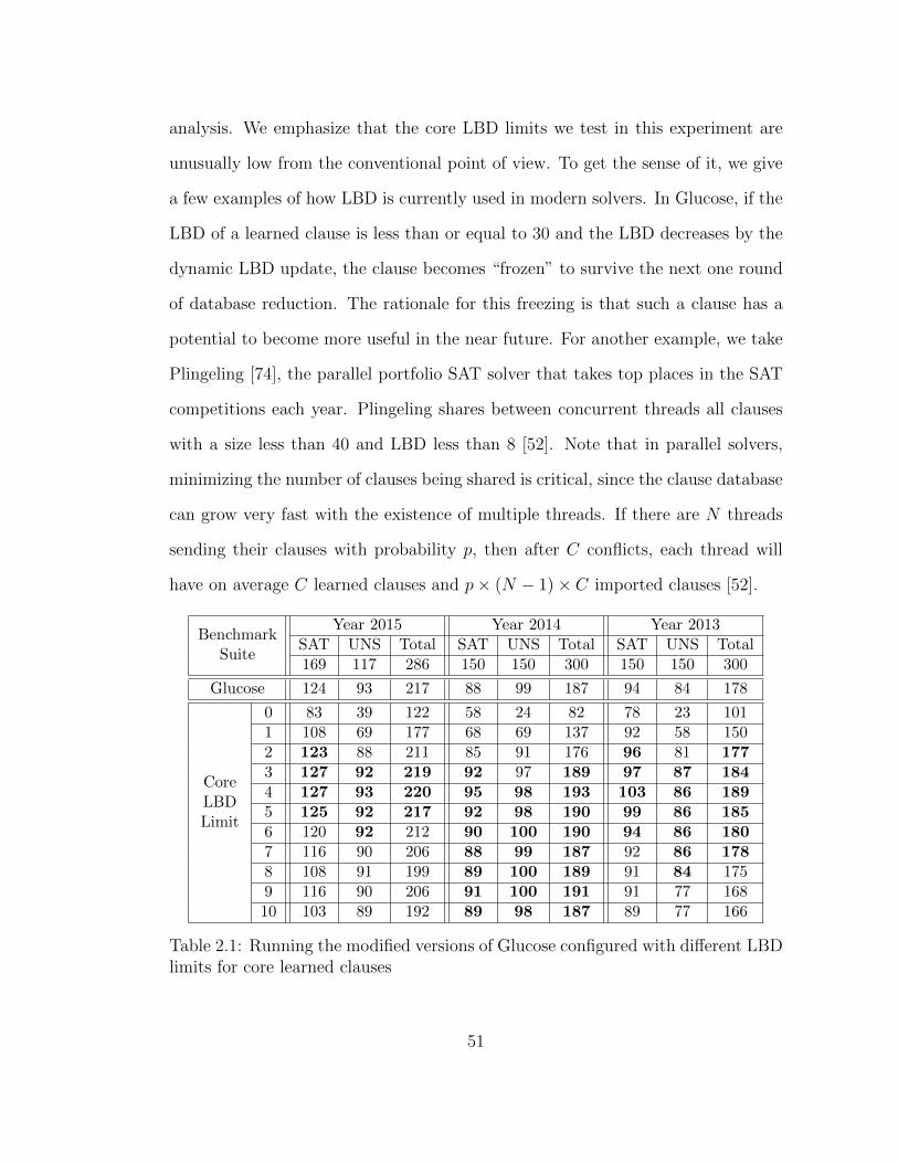
analysis. We emphasize that the core LBD limits we test in this experiment are

unusually low from the conventional point of view. To get the sense of it, we give

a few examples of how LBD is currently used in modern solvers. In Glucose, if the

LBD of a learned clause is less than or equal to 30 and the LBD decreases by the

dynamic LBD update, the clause becomes “frozen” to survive the next one round

of database reduction. The rationale for this freezing is that such a clause has a

potential to become more useful in the near future. For another example, we take

Plingeling [74], the parallel portfolio SAT solver that takes top places in the SAT

competitions each year. Plingeling shares between concurrent threads all clauses

with a size less than 40 and LBD less than 8 [52]. Note that in parallel solvers,

minimizing the number of clauses being shared is critical, since the clause database

can grow very fast with the existence of multiple threads. If there are N threads

sending their clauses with probability p, then after C conflicts, each thread will

have on average C learned clauses and p× (N − 1)× C imported clauses [52].

BenchmarkSuite

Year 2015 Year 2014 Year 2013SAT UNS Total SAT UNS Total SAT UNS Total169 117 286 150 150 300 150 150 300

Glucose 124 93 217 88 99 187 94 84 178

CoreLBDLimit

0 83 39 122 58 24 82 78 23 1011 108 69 177 68 69 137 92 58 1502 123 88 211 85 91 176 96 81 1773 127 92 219 92 97 189 97 87 1844 127 93 220 95 98 193 103 86 1895 125 92 217 92 98 190 99 86 1856 120 92 212 90 100 190 94 86 1807 116 90 206 88 99 187 92 86 1788 108 91 199 89 100 189 91 84 1759 116 90 206 91 100 191 91 77 16810 103 89 192 89 98 187 89 77 166

Table 2.1: Running the modified versions of Glucose configured with different LBDlimits for core learned clauses

51

Table 2.1 shows the result of running Glucose modified in the aforementioned

way, using different core LBD limits. The machine configuration used is the

StarExec cluster (Chapter 1). The timeout is set to 1,800 seconds. The num-

bers in the table are solved problem instances within the timeout. We took the

application benchmark suites used in the past three years’ annual SAT-related

competitive events (SAT Competition 2013, SAT Competition 2014, and SAT-

Race 2015). Each competitive event used 300 application benchmarks, but we

excluded 14 instances from the SAT-Race 2015 as their satisfiability status is not

known to date. The benchmarks are split by their satisfiability status: satisfiable

instances in the SAT column, and unsatisfiable ones in the UNS column. For com-

parison, we included the result of the base solver Glucose in the fourth row. The

bold numbers are the cases where the original Glucose solved at most one more

problem than the modified solver that uses the corresponding core LBD limit. The

intention of the bold numbers is to highlight the comparable performance of the

modified solvers.

Table 2.1 reveals several interesting points. First of all, it clearly shows that

the modified solvers not only work decently but often outperform the base solver.

Fairly consistently, the performance peaks around the LBD limit 4 across the en-

tire benchmark suites and then degrades thereafter. This already confirms that

it is usually sufficient to just accumulate low-LBD clauses in order to solve an

industrial problem and solve it fast. For unsatisfiable instances, this implies that

most real-world problems do have a simple resolution proof tree that can be con-

structed largely out of low-LBD clauses. For satisfiable problems, the LBD limit

of 2 (or sometimes even 1) is already as powerful as the original Glucose. Even

the configuration using the LBD limit of 0 is capable of solving many satisfiable

52

instances. This is very unexpected considering that this configuration can only

have up to 20,000 local clauses with no core clauses at all. Note also that Glucose

has an inherent weakness on satisfiable instances. (We discuss this issue in more

detail in Chapter 3). As we shall see in Chapter 3, it is possible to further mod-

ify this solver with the 0-LBD limit so that it becomes more powerful than the

original Glucose for satisfiable instances. Conclusively, this experiment leads us

to the surprising realization that learned clauses are not as important as they are

normally believed to be. In terms of end results, learned clauses hardly contribute

to solving a real-world problem unless their LBD is critically low, at least in the

current state of the art of CDCL. This is particularly true for satisfiable instances.

It is obvious that the modified solvers are severely limited in that they are inca-

pable of constructing a “sophisticated” refutation proof (i.e., a proof composed of

many high-LBD clauses). We can verify this limitation by observing the increasing

strength on unsatisfiable instances as the LBD limit also increases (but only up to

some point). Even with this limitation, the performance of the modified solvers

are comparable to the performance of the base solver. It is worth mentioning that

the original Glucose is very strong on unsatisfiable instances. For example, Glu-

cose was ranked 1st in 2009, 2nd in 2011, 1st in 2013, and 2nd in 2014 in the

application UNSAT tracks of past competitions. The fact that the unconstrained

base solver does not outperform the modified solvers by a large margin may sug-

gest that CDCL solvers in general are inherently not good at finding sophisticated

proofs efficiently, at least for now. The emphasis in the previous sentence is on

the efficiency, because Glucose at least retains the potential power to find sophis-

ticated proofs, the potential that the modified solvers do not have. However, in

the current state of CDCL, this experimental result suggests that keeping around

53

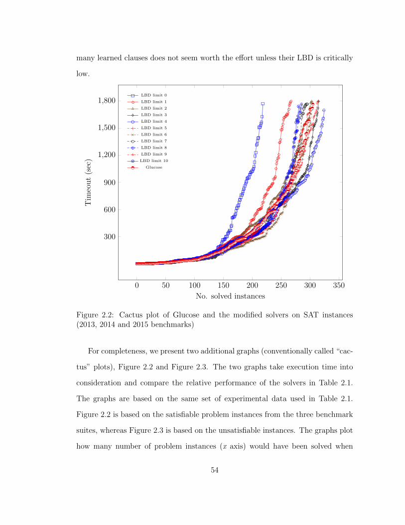
many learned clauses does not seem worth the effort unless their LBD is critically

low.

0 50 100 150 200 250 300 350

300

600

900

1,200

1,500

1,800

No. solved instances

Tim

eout(sec)

LBD limit 0

LBD limit 1

LBD limit 2

LBD limit 3

LBD limit 4

LBD limit 5

LBD limit 6

LBD limit 7

LBD limit 8

LBD limit 9

LBD limit 10

Glucose

Figure 2.2: Cactus plot of Glucose and the modified solvers on SAT instances(2013, 2014 and 2015 benchmarks)

For completeness, we present two additional graphs (conventionally called “cac-

tus” plots), Figure 2.2 and Figure 2.3. The two graphs take execution time into

consideration and compare the relative performance of the solvers in Table 2.1.

The graphs are based on the same set of experimental data used in Table 2.1.

Figure 2.2 is based on the satisfiable problem instances from the three benchmark

suites, whereas Figure 2.3 is based on the unsatisfiable instances. The graphs plot

how many number of problem instances (x axis) would have been solved when

54

0 50 100 150 200 250 300

300

600

900

1,200

1,500

1,800

No. solved instances

Tim

eout(sec)

LBD limit 0

LBD limit 1

LBD limit 2

LBD limit 3

LBD limit 4

LBD limit 5

LBD limit 6

LBD limit 7

LBD limit 8

LBD limit 9

LBD limit 10

Glucose

Figure 2.3: Cactus plot of Glucose and the modified solvers on UNSAT instances(2013, 2014 and 2015 benchmarks)

different timeouts (y axis) were used. Basically, the data shown in the two graphs

are consistent with the results in Table 2.1. That is, even when using different

timeout values, we can still make the same observations as we did from Table 2.1.

Specifically, Figure 2.2 shows that the modified solvers using the core LBD lim-

its of 3, 4 and 5 consistently give better performance than the original Glucose

on satisfiable instances. This consistent performance throughout different time-

out values fortifies our perspective that clauses are not so important unless their

LBD is critically low, particularly for satisfiable instances. Similarly, Figure 2.3

shows that the modified solvers using the LBD limits of 3, 4, 5, 6, 7 and 8 have

55

comparable performance on unsatisfiable instances when timeouts are sufficiently

large.

BenchmarkSuite

Year 2015 Year 2014 Year 2013SAT UNS Total SAT UNS Total SAT UNS Total169 117 286 150 150 300 150 150 300

Glucose 124 93 217 88 99 187 94 84 178

CoreSize

Limit

5 126 86 212 88 83 171 98 75 1737 130 89 219 91 90 181 95 82 1779 129 90 219 91 90 181 97 83 18011 123 92 215 91 91 182 91 83 17413 122 89 211 92 90 182 91 81 17215 121 88 209 94 91 185 94 78 17217 117 89 206 88 92 180 91 78 16919 112 90 202 90 94 184 96 77 173

Table 2.2: Running the modified versions of Glucose configured with different sizelimits for core learned clauses

We also conducted another variant of the experiment. This time, we use the

clause size instead of LBD as the limit for determining the core learned clauses.

Note that, however, we did not change the LBD-based restart strategy of Glu-

cose [29]. This means that, technically, these solvers will abandon the current

search branch and initiate a full restart if it seems that they are learning clauses

whose LBD is greater than the global average. In simple terms, the solvers will still

try to learn clauses with lower-than-average LBD values actively [29]. Table 2.2

shows the experimental results with 8 different size limits, ranging from 5 to 19,

on the same machine configuration as before. As in Table 2.1, the bold numbers

are the cases where the original Glucose solved at most one more problem than

the modified solver. It is very surprising in that, overall, the performance of the

modified solvers is comparable to the the original Glucose. For satisfiable problem

instances, the modified solvers are often better than Glucose, even with very low

size limits. The effectiveness on unsatisfiable instances becomes generally worse,

56

but the performance is still impressive considering the severely limited capability

of the solvers in constructing a resolution proof tree. This impressive performance

proves that most of the real-world problems that we can solve efficiently have a

proof tree with a near-constant maximum width for a great portion of the proof.

Note also that increasing the size limit does not give better results for unsatisfi-

able instances. Combined with the result in Table 2.1, we verify that LBD is a

better metric than clause size for measuring the global usefulness of a clause in

contributing to a proof of unsatisfiability.

0 50 100 150 200 250 300

300

600

900

1,200

1,500

1,800

No. solved instances

Tim

eout(sec)

Size limit 5

Size limit 7

Size limit 9

Size limit 11

Size limit 13

Size limit 15

Size limit 17

Size limit 19

Glucose

Figure 2.4: Cactus plot of Glucose and the modified solvers on SAT instances(2013, 2014 and 2015 benchmarks)

Figure 2.4 and Figure 2.5 are cactus plots based on the data in Table 2.2. The

57

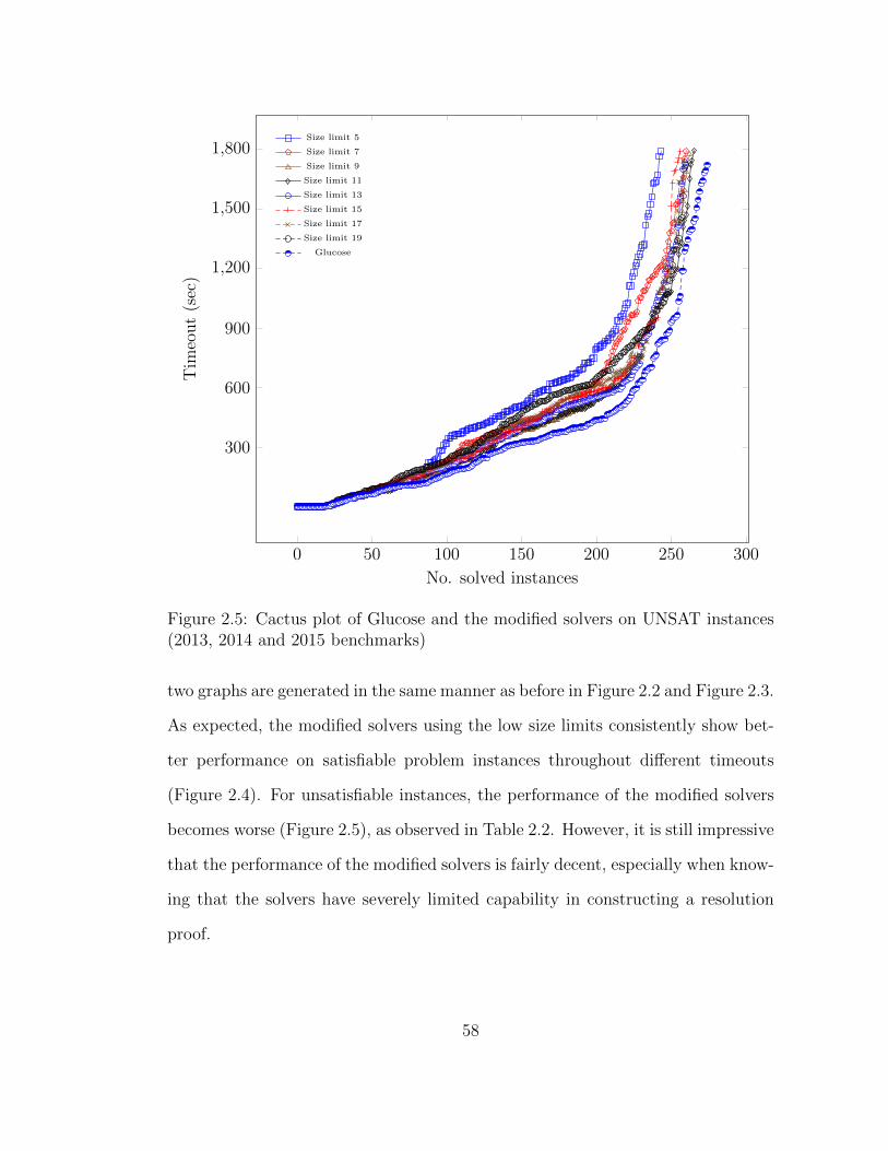
0 50 100 150 200 250 300

300

600

900

1,200

1,500

1,800

No. solved instances

Tim

eout(sec)

Size limit 5

Size limit 7

Size limit 9

Size limit 11

Size limit 13

Size limit 15

Size limit 17

Size limit 19

Glucose

Figure 2.5: Cactus plot of Glucose and the modified solvers on UNSAT instances(2013, 2014 and 2015 benchmarks)

two graphs are generated in the same manner as before in Figure 2.2 and Figure 2.3.

As expected, the modified solvers using the low size limits consistently show bet-

ter performance on satisfiable problem instances throughout different timeouts

(Figure 2.4). For unsatisfiable instances, the performance of the modified solvers

becomes worse (Figure 2.5), as observed in Table 2.2. However, it is still impressive

that the performance of the modified solvers is fairly decent, especially when know-

ing that the solvers have severely limited capability in constructing a resolution

proof.

58

2.3.3 SAT Competition Results

The SAT community organizes many SAT-related competitive events each year.

Over the years, the competitions have significantly contributed to the fast progress

in SAT solver technology that has made SAT a practical success story of computer

science [99, 71]. Our experimental results are consistent with the results of the

past two years’ SAT competitions. Not only do the competition results strongly

support our findings and conclusions described in this chapter, but the results show

that our simple clause management scheme of core and local clauses can also bring

considerable performance improvements.

In 2014, we submitted three prototype solvers to SAT Competition 2014 and

Configurable SAT Solver Challenge (CSSC) 2014 [81]. The purpose of our entries

to these competitive events was to openly challenge the validity of many common

beliefs that stem from the assumption that learned clauses are the most precious

data in CDCL. Basically, these prototypes implemented the above idea of core and

local learned clauses, using the core LBD limit of 5. The names of the solvers are

MiniSat HACK 999ED, MiniSat HACK 1430ED, and SWDiA5BY [82]. As the

name suggests, the former two are based on MiniSat. SWDiA5BY is based on

Glucose and hence very similar to the very solver we used in our previous exper-

iments (differs only in a minor way). Particularly, the 999ED version was eligible

for entering the MiniSat hack track in SAT Competition 2014, where only hacked

MiniSat solvers are allowed to compete. Because only a small degree of changes to

MiniSat is permitted as a rule, MiniSat hack solvers in this track are normally not

expected to be competitive with state-of-the-art solvers competing in the main

track4. Our MiniSat hack solvers were very successful: the 999ED version won

4However, we managed to implement some of the most critical features of Glucose in Min-

59

a gold medal in the MiniSat hack track of SAT Competition 2014, and a silver

medal in the industrial track of CSSC 2014. A comprehensive report on CSSC

2014 showed that the 999ED version would be the top-performing solver if all the

participating solvers used default parameters [81]. Not only that, the MiniSat hack

solvers took 5th and 11th (among 38 solvers) in the application SAT track, 4th

and 5th (among 15) in the application UNSAT track, 5th and 7th (among 42) in

the hard-combinatorial SAT track, and 9th (among 34) in the hard-combinatorial

SAT+UNSAT track of SAT Competition 2014, despite the high intensity of com-

petition in these tracks. SWDiA5BY was even more successful: 2nd, 3rd, and

3rd in the application SAT+UNSAT, SAT, and UNSAT track, respectively. Later

studies revealed that SWDiA5BY would have been the top-performing solver if

lower timeouts had been used [81]. The result of SWDiA5BY in the competition is

consistent with the data in Table 2.1. The table already showed that, particularly

for satisfiable problem instances, we can reliably improve the performance of the

most recent Glucose using the LBD limits around 4 or 5. Conclusively, the com-

petition proved that the strategy to use only low-LBD clauses can actually make

a solver as powerful as any state-of-the-art solvers.

In 2015, we submitted another proof-of-concept solver [27] to SAT-Race 2015.

The solver is derived from SWDiA5BY, and we will describe the details of the

solver in the following chapters in this thesis. We mention the solver briefly here,

because the solver had a particular purpose of emphasizing and advocating our

unconventional perspective on learned clauses in a much more explicit way than

SWDiA5BY does. As a proof-of-concept solver, we intentionally configured it to

have an extreme limit for the core clauses: either the clause size is less than or

iSat HACK 999ED, in addition to our idea of core and local clauses. As such, our MiniSat hacksolvers are much closer to Glucose rather than MiniSat.

60

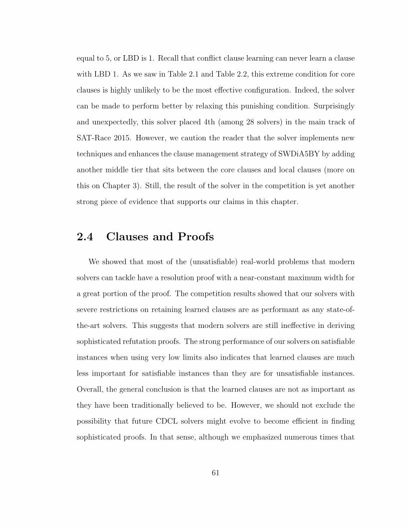
equal to 5, or LBD is 1. Recall that conflict clause learning can never learn a clause

with LBD 1. As we saw in Table 2.1 and Table 2.2, this extreme condition for core

clauses is highly unlikely to be the most effective configuration. Indeed, the solver

can be made to perform better by relaxing this punishing condition. Surprisingly

and unexpectedly, this solver placed 4th (among 28 solvers) in the main track of

SAT-Race 2015. However, we caution the reader that the solver implements new

techniques and enhances the clause management strategy of SWDiA5BY by adding

another middle tier that sits between the core clauses and local clauses (more on

this on Chapter 3). Still, the result of the solver in the competition is yet another

strong piece of evidence that supports our claims in this chapter.

2.4 Clauses and Proofs

We showed that most of the (unsatisfiable) real-world problems that modern

solvers can tackle have a resolution proof with a near-constant maximum width for

a great portion of the proof. The competition results showed that our solvers with

severe restrictions on retaining learned clauses are as performant as any state-of-

the-art solvers. This suggests that modern solvers are still ineffective in deriving

sophisticated refutation proofs. The strong performance of our solvers on satisfiable

instances when using very low limits also indicates that learned clauses are much

less important for satisfiable instances than they are for unsatisfiable instances.

Overall, the general conclusion is that the learned clauses are not as important as

they have been traditionally believed to be. However, we should not exclude the

possibility that future CDCL solvers might evolve to become efficient in finding

sophisticated proofs. In that sense, although we emphasized numerous times that

61

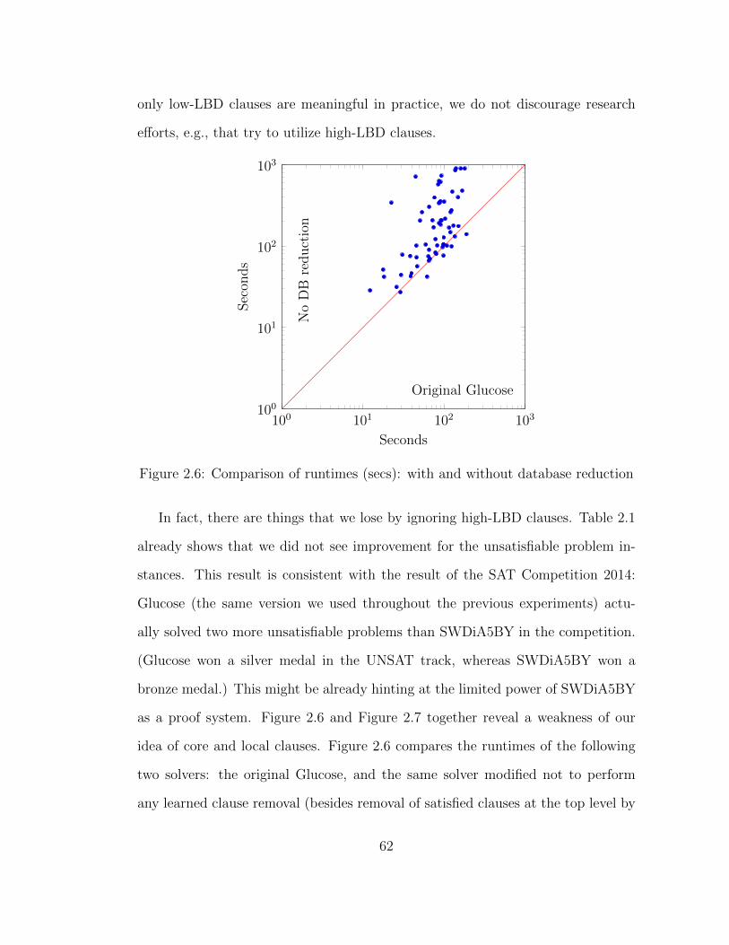
only low-LBD clauses are meaningful in practice, we do not discourage research

efforts, e.g., that try to utilize high-LBD clauses.

100 101 102 103100

101

102

103

Original Glucose

NoDB

reduction

Seconds

Secon

ds

Figure 2.6: Comparison of runtimes (secs): with and without database reduction

In fact, there are things that we lose by ignoring high-LBD clauses. Table 2.1

already shows that we did not see improvement for the unsatisfiable problem in-

stances. This result is consistent with the result of the SAT Competition 2014:

Glucose (the same version we used throughout the previous experiments) actu-

ally solved two more unsatisfiable problems than SWDiA5BY in the competition.

(Glucose won a silver medal in the UNSAT track, whereas SWDiA5BY won a

bronze medal.) This might be already hinting at the limited power of SWDiA5BY

as a proof system. Figure 2.6 and Figure 2.7 together reveal a weakness of our

idea of core and local clauses. Figure 2.6 compares the runtimes of the following

two solvers: the original Glucose, and the same solver modified not to perform

any learned clause removal (besides removal of satisfied clauses at the top level by

62

0 10 20 30 40 50 60 70−100

−50

0

50

100

Problem instance

Diff

eren

ce(%

)

Figure 2.7: Difference in no. conflicts (%): with and without database reduction

trivial simplification). The intention of retaining all learned clauses in the modified

solver is to check the potential advantages of clauses in general. We used a short

timeout of 900 seconds on the machine configuration C (Chapter 1). The 66 bench-

marks were selected out of the unsatisfiable instances from the application tracks

of SAT Competitions 2013 and 2014. (The reason that we consider unsatisfiable

instances only will become clear in Chapter 3. Briefly speaking, learned clauses

are nevertheless unimportant for satisfiable instances.) We selected easy problems

that Glucose solved in roughly between 15 and 200 seconds according to the actual

competition data (excluding some instances that are too big). Almost all other

solvers in the competitions solved the problems very efficiently too. As we shall

see, this experimental setup is sufficient to reveal the general role of clauses as well

as the potential advantages of high-LBD clauses. Because these are easy problems,

someone may expect that the modified Glucose, which does not remove clauses,

63

would still be able to solve the problems efficiently. Perhaps, the modified Glucose

might solve many of the problems more efficiently as the original Glucose is al-

ready removing clauses very aggressively. However, the result is that the modified

solver usually takes more time to solve a problem. This is not surprising especially

after knowing that what matters most is the small number of low-LBD clauses.

From this result, we may hastily conclude that keeping all learned clauses does

not bring any advantage. However, this is not strictly true. Figure 2.7 plots the

difference (%-increase) in the number of conflicts required to solve a problem af-

ter disabling clause removal. For example, if the original Glucose required 40,000

conflicts before returning an answer while the modified Glucose required 30,000

conflicts, the %-increase difference is -25% (i.e., a negative value). We can see that

the modified solver generally requires far fewer conflicts than Glucose to derive a

proof of unsatisfiability. This reduction of required conflicts makes sense because

CDCL solvers derive an empty clause (i.e., a final proof of unsatisfiability) by

successive resolutions based on existing clauses. It is obvious that solvers become

very inefficient if they do not remove clauses at all as we can verify in Figure 2.6.

However, Figure 2.7 suggests that keeping all clauses can actually make a solver

construct a resolution proof “faster” in terms of required conflicts. More than that,

the modified solver may be more capable of deriving sophisticated proofs than the

original Glucose in practice (although in theory they are equally powerful as a

proof system). Similarly, our idea of focusing only on low-LBD clauses may be

inherently limited in that it loses the potential to construct sophisticated proofs.

At the current state, it is very difficult for anyone to provide a decisive reason

why a solver should have improved performance when removing clauses aggres-

sively. As already mentioned in Section 2.2, the reason for the efficiency could be

64

multi-fold. Whatever the reason is, Figure 2.7 suggests the following: we may be

able to achieve significant performance improvement if we could somehow make

solvers retain the similar speed of hitting conflicts while keeping a lot of clauses

(for unsatisfiable instances). Unfortunately, however, it seems that retaining the

similar rate of conflicts is not really viable in practice at the present moment.

Lastly, we showed that what matters most is the low-LBD clauses. Therefore,

someone may naturally conjecture that speeding up the accumulation of low-LBD

clauses would lead to improved performance. We emphasize that this cannot al-

ways be true. There exist ways to boost the speed of generating a lot of low-LBD

clauses dramatically. There even exist problems for which we were able to greatly

speed up learning a lot of unit clauses (i.e., absolute facts to be asserted at the top

level before making any branching decisions). Certainly, having a lot of low-LBD

clauses can help in a general sense. However, those low-LBD clauses can help only

if they actually contribute to constructing a particular resolution proof.

65

Chapter 3

Satisfiability and Unsatisfiability

Proving satisfiability is different from proving unsatisfiability. The inherent dif-

ference between the two is well-known especially in theoretical contexts. One way

to show that a given propositional formula is satisfiable is to present a satisfying

assignment (also called a certificate or a witness in the context of complexity the-

ory) for the variables in the formula. There may exist many satisfying assignments

for a given formula, but one witness is sufficient to prove the satisfiability of the

formula. Obviously, every satisfiable formula has a witness whose size is polyno-

mially bounded with respect to the total number of variables. On the other hand,

to show that a given formula is unsatisfiable, we have to show the non-existence of

any witness. In other words, we need a proof that every possible assignment falsi-

fies the formula. One naive way to prove unsatisfiability is to test every possible

assignment. Of course, there can be other forms of proof for showing unsatisfiabil-

ity. Some proofs can be “short”, i.e., verifiable in polynomial time. Unfortunately,

it is not known to date whether every unsatisfiable formula can have a short proof.

From the complexity theoretic point of view, the problem of showing satisfia-

66

bility of a formula is in the complexity class of NP. Proving unsatisfiability as a

complementary problem to the former problem is not obviously seen to be in NP.

In fact, we have another complexity class defined for this complementary relation:

co-NP. We do not know whether proving satisfiability is easier or more difficult

than proving unsatisfiability, since this is essentially the question of NP = co-NP.

However, it is normally believed that the two sets (NP and co-NP) are different.

There always exists a polynomial-length witness for any satisfiable formula, but it

is generally believed that not every unsatisfiable formula can have a short proof.

It is not hard to imagine that this inherent and fundamental difference between

the two complementary problems naturally extends to practical SAT solving. A

CDCL SAT solver is often viewed as a backtracking algorithm, especially in a prac-

tical setting. However, a solver can also be seen as a propositional proof system

for proving unsatisfiability in a theoretical sense. It is well-known that the broad

class of CDCL solvers as a proof system is as powerful as general resolution [23].

Unfortunately, general resolution is not the most powerful proof system for propo-

sitional satisfiability. There exist other and more powerful propositional proof

systems than general resolution [39]. In other words, CDCL is already limited in

its power to prove unsatisfiability. In fact, it is well-known that there exist certain

classes of problems (e.g., pigeon-hole) for which CDCL solvers are “hopeless” in

proving their unsatisfiability (i.e., any resolution refutation proof will be exponen-

tial in size) [22, 24, 25]. On the other hand, CDCL solvers are not limited at all in

efficient proving of satisfiability. For satisfiable formulas, regardless of the type or

the size of the problem, there is always a possibility that some CDCL solvers can

solve the problem efficiently.

In this chapter, in the context of practical SAT solving, we show that the way

67

CDCL solvers find a satisfying assignment is indeed different from the way they de-

rive a refutation proof of unsatisfiability. We give empirical evidence that highlights

the different nature of solver workings for proving satisfiability and unsatisfiability.

We show that certain elements of CDCL impact solver performance with different

consequences for satisfiable problems and unsatisfiable problems. Specifically, we

describe the different impacts in terms of varying degrees of roles and effects of

some of the most important elements in CDCL: learned clauses, restarts, and the

VSIDS heuristic. Consequently, we reveal new and fresh insights about the internal

workings of a SAT solver. Analyzing the different impacts of these elements, we

give partial explanations about the reasons for the different workings of a solver.

In addition to the explanations for the SAT/UNSAT difference, we also pro-

pose ideas for exploiting the difference to improve performance on both satisfiable

and unsatisfiable problems. Unfortunately, we observe that there exist adverse

forces between SAT and UNSAT: aiming at satisfiable (or unsatisfiable) problem

instances weakens the strength for unsatisfiable (or satisfiable) instances. However,

careful exploitation of the difference can bring improvement on both satisfiable and

unsatisfiable problems. To show the viability of such exploitation, we implemented

on top of Glucose a few simple ideas that leverage the newly gained insights about

the SAT/UNSAT difference. Our experiments and the results of SAT-Race 2015

confirm that these ideas bring substantial performance improvements.

Therefore, our work advances the state of the art of CDCL by a perceivable

margin. The degree of the advancement is substantial in that, according to the

SAT-Race 2015 results, the CDCL engine itself implementing our simple ideas

becomes competitive with any state-of-the-art SAT solvers, even solvers with a

huge code base that implement complex features outside CDCL.

68

Lastly, we remind the reader that all the arguments in this thesis apply only

to real-world problems.

3.1 Background

The general idea that one can have a specialized tactic to tackle a certain kind

of problem to have better performance is not new. Even if we limit our scope to

the recently established discipline of practical SAT solving, the idea to develop

specialized methods for either satisfiable or unsatisfiable problems dates back to

1996 [83]. The goals of the work in [83] are to develop specialized solvers that work

better for either SAT or UNSAT. Our motivation and our work shares basically the

same high-level perspective, but we focus more on the analysis and comprehension

of the difference between SAT and UNSAT. Moreover, our ultimate goal is to

achieve performance improvement in both SAT and UNSAT cases by exploiting

the SAT/UNSAT difference. After all, the work in 1996 was based on DPLL

without CDCL. Since then, we have witnessed impressive progress in practical

SAT research, and thus their work does not apply in the context of today’s modern

CDCL solvers.

Since then, in the course of developing practical SAT solvers, there has been

little work that explores the same idea of conceiving specialized methods to specif-

ically target either SAT or UNSAT. More than that, much of the work on practi-

cal SAT does not consider the inherently different solver behavior, depending on

whether a given formula is satisfiable or not. We can find numerous instances of

such examples where the difference between SAT and UNSAT is not taken into

consideration at all. Of course, there does exist work where experiments are evalu-

69

ated separately according to the SAT or UNSAT status. However, in most of these

cases, the SAT/UNSAT difference is not taken into account while designing algo-

rithms or setting up evaluation methodologies in the first place. As a result, such

work often ends up superficially reporting observed numbers just classified by the

SAT or UNSAT status. The consequence of failing to consider the SAT/UNSAT

difference is not just missed opportunities for potential improvements of a SAT

solver. We will see soon that this failure has actually caused an inadvertent re-

gression in the recent advancements in SAT research.

The central theme of this chapter is that the way CDCL SAT solvers find a

satisfying assignment is very different from the way they prove unsatisfiability in

practice. Although the fact itself is not new, not much research has been done to

understand how and why solvers work differently and what can be done accordingly

to realize improvements. As such, speculating the answers to the above questions

is basically uncharted territory. In this chapter, we give partial explanations to

the above questions from certain aspects. Understanding the reasons for the differ-

ence will not only be interesting from the theoretical perspective in explaining the

internal workings of CDCL but will also allow us to exploit the difference in an ef-

fective way to bring further improvements. As a proof of concept, we implemented

simple techniques based on our reasoning about the SAT/UNSAT difference in

our new solver COMiniSatPS [27]. Particularly, the most recent SAT competitive

event (SAT-Race 2015) confirms that our solver brings significant performance

improvements.

The main contributions of this work are summarized as follows:

1. Analysis and comprehension of the SAT/UNSAT difference. It

is well-known that CDCL solvers work differently on satisfiable and unsatisfiable

70

problems. However, today’s solvers are far from leveraging this difference to the

fullest degree. This is because how and why they are different has not been ex-

plained much. We provide explanations for the difference. We support our claims

with a wide range of concrete evidence. The main evidence is the varying roles and

effects of some of the most important elements in CDCL: learned clauses, restarts,

and the VSIDS heuristic. The evidence additionally gives fresh insights on the

workings of these elements in CDCL.

2. Promoting attention to the SAT/UNSAT difference. Historically,

the effects of algorithms and techniques have not been analyzed separately on

SAT and UNSAT instances on many occasions, or if so, only superficially. How-

ever, because of the inherent difference in proving SAT and UNSAT, there is a

good chance that one technique can be slightly good on SAT (or UNSAT) but

considerably bad on UNSAT (or SAT). In that case, such a technique may easily

be discarded because of the overall worse result. Therefore, paying attention to the

possible consequences of the SAT/UNSAT difference is important. Moreover, there

are many indications that research work on SAT is not recognizing the potential of

exploiting the SAT/UNSAT difference. As a representative example, in the SAT

Competition 2014, every practical SAT solver used the same executable binary for

both SAT and UNSAT tracks1, except ROKK2 [91]. As another example, SAT-

Race 2015 did not have an independent SAT or UNSAT track but had a single

main track. The main track even used an unequal number of SAT and UNSAT

problem instances. We encourage more in-depth research for exploring potential

1Some solvers disabled certain complex simplification techniques in the UNSAT track. How-ever, this was only because the solvers cannot generate verifiable proofs when such techniquesare used.

2However, the ROKK version specialized for SAT was simply a tuned version with severalparameter adjustments.

71

ways to exploit the SAT/UNSAT difference. We suggest that at least techniques

and solvers should be carefully evaluated with the SAT/UNSAT difference in mind.

3. Performance improvements. First, we will come to understand how to

make a solver stronger on SAT at the expense of making it weaker on UNSAT

(and vice versa). The fact that we can build efficient solvers specialized for either

SAT or UNSAT immediately benefits us in practice, e.g., by allowing us to run

the two specialized solvers concurrently. Furthermore, we show the potential of

exploiting the SAT/UNSAT difference for achieving improvements on both SAT

and UNSAT. Ultimately, we confirm this potential by presenting concrete results

of improved performance with our new solver that implements several new ideas

to exploit the SAT/UNSAT difference.

4. Uncovering potential value of neglected techniques. Our supporting

evidence includes an explanations for the effectiveness (and ineffectiveness) of the

Luby series [50] restart strategy. The Luby strategy is considered old in that

modern SAT solvers rarely use it3. The use of the Luby strategy in a solver

normally indicates that the solver is falling behind with the progress in SAT solving.

In modern solvers, much more rapid restarts (e.g., Glucose-style restarts [29])

replaced the Luby strategy. This is because rapid restarts are empirically shown

to be far superior to Luby restarts in an ultimate sense. However, we show that

the slow Luby restarts are superior to rapid restarts if restricted to satisfiable

instances. The case of the Luby strategy is an example of a technique from the

past being overshadowed and discarded easily in favor of new but incompatible

techniques. A new technique could be strictly superior to an old technique in an

overall sense. However, it is possible that the old technique is stronger on SAT (or

3We refer to the Luby restarts with much lower frequency when compared to recent rapidrestarts, e.g., the Luby series used in MiniSat.

72

UNSAT), and only on SAT (or UNSAT), than the new technique. Like in the Luby

case, revisiting past and current research work with the SAT/UNSAT difference in

mind may reveal new insights. In the same vein, we uncover some interesting ideas

hidden in the results of the past SAT Competitions in the course of our discussion.

3.2 Satisfiability and Unsatisfiability in CDCL

We first explain the different solver workings between finding a SAT solution

and deriving an UNSAT proof. We present and analyze empirical data that high-

light the different natures of SAT and UNSAT. We discuss in detail the varying

degrees of roles and effects of learned clauses, restarts and the VSIDS heuristic,

depending on whether the problem is satisfiable or unsatisfiable. Ultimately, we

propose new ideas to exploit the SAT/UNSAT difference to achieve improvements

on both SAT and UNSAT.

3.2.1 Learned Clauses

There have been many works that studied the theoretical power and limitation

of CDCL, e.g., by defining a formal model for CDCL. These works tend to see

CDCL as a formal proof system from the complexity-theoretic point of view. It is

well-known that the broad class of CDCL solvers are as powerful as general reso-

lution [23]. Fundamentally, resolution works on clauses. CDCL solvers also work

only on clauses by their design. Everything that happens inside a standard CDCL

solver can be expressed in terms of resolution. For example, unit propagation is

a special case of the resolution rule, a new conflict clause is learned by applying

resolutions in a series, and the same applies for various kinds of clause simplifi-

73

cations and modifications. In fact, the resolution rule is a powerful inference rule

that can generalize a lot of high-level deductions, including modus ponens. When

seeing a CDCL solver as a proof system, the focus is on the resolution rule and

hence the complexity of the resolution-based refutation proof. In other words, the

focus is on the system’s capability to refute a given theory (i.e., an input formula)

in a highly theoretical context.

In a related but slightly more practical context, there exists another perspective

where a solver is seen as a clause producer [85]. This perspective puts a particular

emphasis on clauses. Specifically, this perspective focuses on the aspect of generat-

ing new clauses primarily by conflict analysis. In this perspective, a solver is seen

as a system that continuously derives (learns) new clauses from existing clauses by

applying resolutions, which is exactly what happens in a solver. If a solver derives

an empty clause, it has proved unsatisfiability of the input formula. Specifically,

the moment that a solver derives an empty clause is when a conflict occurs at the

top decision level. This perspective of seeing a solver as a clause producer also has

a focus on clauses.

From these arguments, it is not difficult to see that learned clauses are the

elemental building blocks for constructing a resolution-based refutation proof of

unsatisfiability. In a more realistic sense, the resolution-based proof is a directed

acyclic graph where nodes are clauses, edges represent application of resolution,

and one of the nodes is an empty clause. In other words, learned clauses in CDCL

solvers play an important role as a participant in a final proof, in the case of

unsatisfiable formulas. (However, as a reminder, we emphasize that the importance

of learned clauses is significantly limited in practice as we showed in Chapter 2.)

On the other hand, we hypothesize that learned clauses do not play an impor-

74

tant role in finding a solution for satisfiable formulas. A hypothetical solver that

always makes a perfect decision can find a satisfying assignment in polynomial

time without ever learning a new conflict clause. In this theoretical sense, there

is no limitation in efficient finding of a solution for satisfiable formulas. Moreover,

we may not need learning clauses at all to find a solution. A real example is a local

search algorithm, which is incapable of proving unsatisfiability. In contrast, there

exist limitations of CDCL solvers in proving unsatisfiability. It has been shown

that certain classes of problems (e.g., the pigeon-hole problem) are intractable for

CDCL solvers [22, 24, 25], e.g., because their resolution-based refutation proofs

have to be exponential in size.

It is well-known that clause learning is the technique in CDCL that has the

greatest relative importance in CDCL [76]. As such, it is easy to assume that

learned clauses are equally useful and important in CDCL solvers for both satisfi-

able and unsatisfiable formulas in practice. We show in this chapter that learned

clauses have a different degree of importance for satisfiable and unsatisfiable for-

mulas; learned clauses are much less relevant for satisfiable formulas than for un-

satisfiable formulas.

As an interesting side note regarding the intractable problems for CDCL, the

pigeon-hole problems have appeared in the past annual SAT competitions. Par-

ticularly, the 2013 competition contained about 14 (13 being the pigeon-hole) un-

satisfiable problems that are intractable with resolution. As expected, no solvers4

in the competition were able to solve the problems despite their tiny size (i.e., a

4There were two exceptions: Lingeling [74] and BreakIDGlucose [84]. Lingeling has a spe-cialized deduction based on cardinality constraints and solved all 14 problems in a fraction ofa second; BreakIDGlucose detects symmetries in an input formula and adds extra clauses thatbreak the symmetries in the preprocessing step. However, both solvers were not able to solve theproblems in the certified UNSAT track either, where solvers are required to generate a verifiableproof.

75

small number of pigeons and holes).

3.2.1.1 A Short Survey

100 101 102 103100

101

102

103

Original Glucose

NoDB

reduction

Seconds

Secon

ds

Figure 3.1: Comparison of runtimes with and without clause database reductionon 69 SAT instances

We start the discussion by presenting a short survey. The survey is limited

but sufficient to uncover the different roles of learned clauses in SAT and UNSAT

problems. For this survey, we used the most recent version of Glucose as a base

solver (the same solver that we used in the previous chapter). We run and com-

pare two solvers in this survey: 1) the original Glucose; and 2) Glucose modified

not to perform periodic clause database reduction. In other words, the modified

solver does not remove any learned clauses (unless they are trivially satisfied).

We performed the experiment on the machine configuration B (Chapter 1) with a

short timeout of 900 seconds. We used 135 benchmark problems from SAT Com-

76

100 101 102 103100

101

102

103

Original Glucose

NoDB

reduction

Seconds

Secon

ds

Figure 3.2: Comparison of runtimes with and without clause database reductionon 66 UNSAT instances

petitions 2013 and 2014. We selected easy problems that Glucose solved roughly

between 15 and 200 seconds according to the competition data (excluding some

that are too big). All other solvers in the competitions (except a few solvers that

are disqualified or showed overall very poor performance) were able to solve the

problems very efficiently too. Possible expectations with the modified Glucose

on these easy problems could be that the solver would still be able to solve the

problems efficiently, or sometimes more efficiently as the original Glucose may be

removing clauses too aggressively. Figure 3.1 and Figure 3.2 show results of run-

ning the solvers. In fact, Figure 3.2 with 66 UNSAT problem instances is exactly

the same graph as Figure 2.6. In the previous chapter, we used the graph to show

the degraded performance of the modified solver. Here, we present the graph to-

gether with one for SAT instances. With these two graphs, now the emphasis is

77

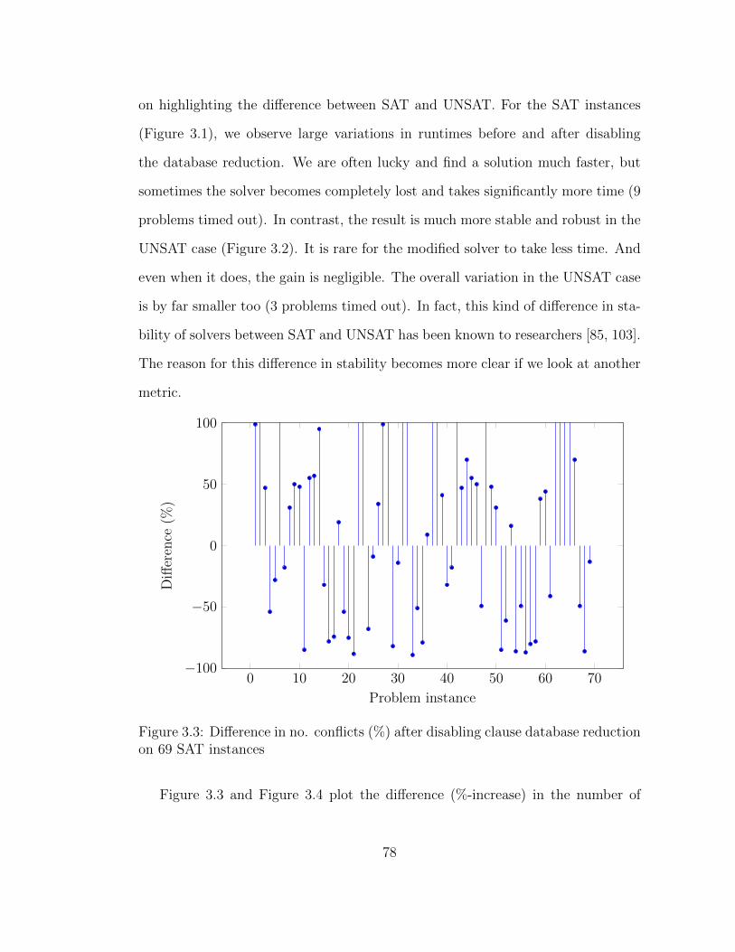
on highlighting the difference between SAT and UNSAT. For the SAT instances

(Figure 3.1), we observe large variations in runtimes before and after disabling

the database reduction. We are often lucky and find a solution much faster, but

sometimes the solver becomes completely lost and takes significantly more time (9

problems timed out). In contrast, the result is much more stable and robust in the

UNSAT case (Figure 3.2). It is rare for the modified solver to take less time. And

even when it does, the gain is negligible. The overall variation in the UNSAT case

is by far smaller too (3 problems timed out). In fact, this kind of difference in sta-

bility of solvers between SAT and UNSAT has been known to researchers [85, 103].

The reason for this difference in stability becomes more clear if we look at another

metric.

0 10 20 30 40 50 60 70−100

−50

0

50

100

Problem instance

Diff

eren

ce(%

)

Figure 3.3: Difference in no. conflicts (%) after disabling clause database reductionon 69 SAT instances

Figure 3.3 and Figure 3.4 plot the difference (%-increase) in the number of

78

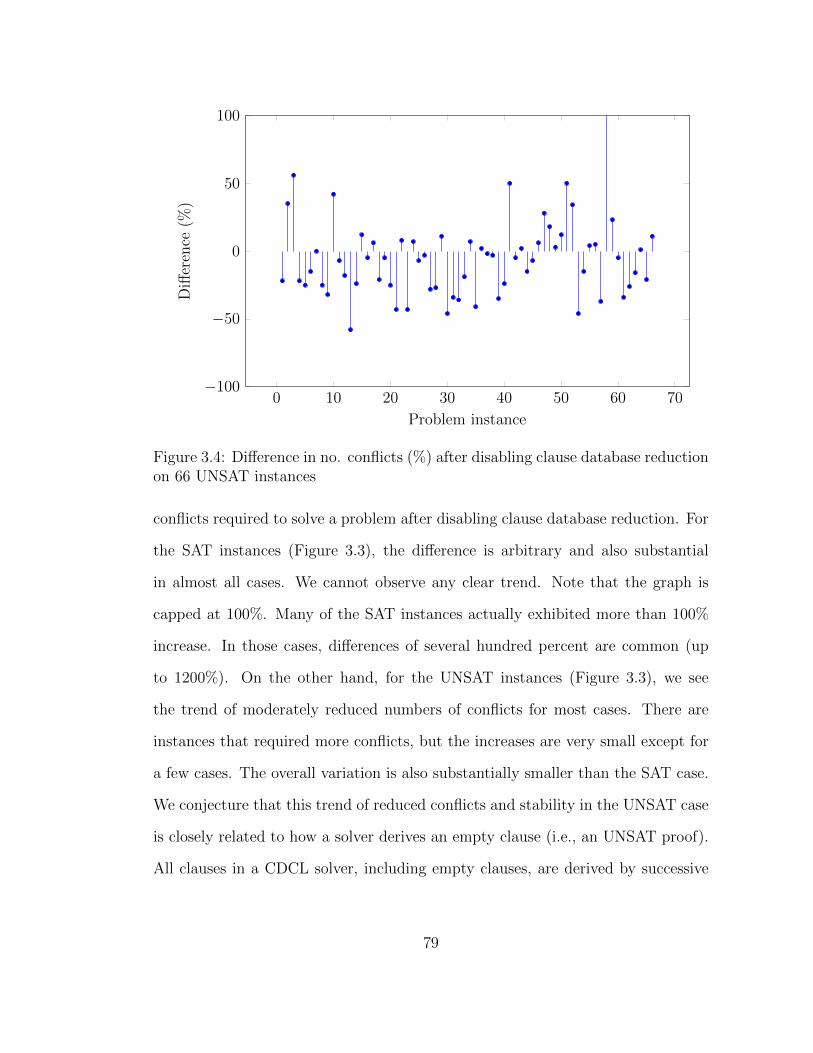
0 10 20 30 40 50 60 70−100

−50

0

50

100

Problem instance

Diff

eren

ce(%

)

Figure 3.4: Difference in no. conflicts (%) after disabling clause database reductionon 66 UNSAT instances

conflicts required to solve a problem after disabling clause database reduction. For

the SAT instances (Figure 3.3), the difference is arbitrary and also substantial

in almost all cases. We cannot observe any clear trend. Note that the graph is

capped at 100%. Many of the SAT instances actually exhibited more than 100%

increase. In those cases, differences of several hundred percent are common (up

to 1200%). On the other hand, for the UNSAT instances (Figure 3.3), we see

the trend of moderately reduced numbers of conflicts for most cases. There are

instances that required more conflicts, but the increases are very small except for

a few cases. The overall variation is also substantially smaller than the SAT case.

We conjecture that this trend of reduced conflicts and stability in the UNSAT case

is closely related to how a solver derives an empty clause (i.e., an UNSAT proof).

All clauses in a CDCL solver, including empty clauses, are derived by successive

79

resolutions based on other existing clauses. Figure 3.4 shows that fewer conflicts

are required in general when we keep every learned clause. In other words, learned

clauses are certainly useful for proving unsatisfiability. An implication of Figure 3.4

is that, if we could somehow make a solver maintain the same speed of hitting

conflicts, keeping every clause would generally bring substantial improvement on

UNSAT problems. On the contrary, this argument does not hold for SAT instances.

Figure 3.3 shows that learned clauses are not relevant for improving efficiency in

finding a solution for SAT instances. Rather, keeping every clause may adversely

make a solver very unstable as we can see in this survey.

3.2.1.2 Varying Roles of Learned Clauses

We now present empirical evidence that learned clauses play a surprisingly

insignificant role in the SAT case in contrast to the UNSAT case.

In fact, such evidence was already presented in the previous chapter, in Ta-

ble 2.1 and Table 2.2. We do not duplicate the tables in this section. Instead, we

give a brief analysis of the data in the tables here. This time, the focus of our

analysis is on highlighting the different impact of keeping learned clauses on SAT

and UNSAT instances. The difference between SAT and UNSAT is particularly

conspicuous when small LBD or size limits for core clauses (Chapter 2) are used

(i.e., when the solver is severely constrained in keeping learned clauses). For ex-

ample, when using the LBD limit of 0 or 1, the modified solvers were able to solve

surprisingly many SAT problems, sometimes a similar number of problems as the

original Glucose. In contrast, the performance on UNSAT problems with these low

LBD limits is significantly poor. We can observe a similar trend in Table 2.2 too;

for the low size limit for core clauses, the performance on SAT problems is always

80

better than the original Glucose, but it is much worse on UNSAT problems.

In this section, we perform a new experiment to present more empirical evidence

that shows a similar trend. Similar to the experimental setup of Table 2.1, we run

solvers with different LBD limits. This time, however, we use a different solver

than the original Glucose and on a different execution environment. Based on

SWDiA5BY (Chapter 2), we implemented a new hybrid strategy whose description

will be given later in Section 3.2.2 of this chapter. We do not describe the new

techniques here, since it is irrelevant for the purpose of highlighting the different

effects of learned clauses for SAT and UNSAT. Nonetheless, except for the new

hybrid strategy, the new solver we use in this experiment is almost identical to

SWDiA5BY. The only other modification is that the new solver can have up to

30,000 local clauses (increased from 20,000). As in Table 2.1, we tested using

different LBD limits for the core clauses with the new solver.

SWDiA5BY SWDiA5BY + Hybrid StrategyCore LBD limit 5 0 1 2 3 4 5 6

SAT 109 120 131 129 129 124 129 1282013 UNSAT 123 47 88 113 116 120 126 122

Total 232 167 219 242 245 244 255 250

SAT 88 88 93 91 92 90 90 952011 UNSAT 104 73 92 97 97 101 101 99

Total 192 161 185 188 189 191 191 194

Table 3.1: No. solved instances with different LBD core limits on 600 benchmarksfrom SAT Competition 2013 and 2011

Table 3.1 shows results of running the new solver (denoted by SWDiA5BY

+ Hybrid Strategy) on the 2013 and 2011 SAT Competition benchmarks. Each

of the benchmark suites from the two competitions contains 150 SAT and 150

UNSAT instances (i.e., 600 benchmark instances as a whole). We used a timeout

of 4,200 for the 2013 competition benchmarks and 1,500 seconds for the 2011

81

benchmarks on the machine configuration B (Chapter 1). The smaller timeout for

the 2011 benchmarks is due to our resource constraints, but the data is sufficient

to highlight the different effects of learned clauses between SAT and UNSAT.

Note that, as with SWDiA5BY, the new solver using the core LBD limit of 0

does not have any core clauses; this solver can have up to 30,000 local clauses only.

The maximum limit of 30,000 clauses is indeed very low as solvers routinely learn

thousands of clauses per second. Observe that this solver configuration can solve in-

credibly many SAT problems. We even observed that for certain SAT benchmarks

(e.g., 001-010.cnf from the 2013 competition), this “unreasonable” configuration

is exceptionally effective and almost optimal. In contrast, the performance of this

solver configuration is very poor on the UNSAT instances and particularly disas-

trous with the 2013 competition benchmarks. Next, consider the results when the

LBD limit is increased by 1. Note that a clause can never be learned with LBD 1.

The LBD value of 1 is observable only when Glucose dynamically updates LBD for

the clauses involved in later conflict analysis, in which case the solver learns a unit

clause and backtracks to the top decision level (i.e., a full restart is performed). In

other words, using the LBD limit 1 is still a highly impractical configuration. Note

the the dramatic improvement to the 0-LBD-limit configuration on the UNSAT

instances. The LBD limit 2 further increases the performance on UNSAT (al-

though the degree of the improvement is less dramatic). These results show that

learned clauses are far more important for proving unsatisfiability than for finding

a solution. This does make sense when considering how a CDCL solver derives an

empty clause with resolution. In contrast, learned clauses play a far less significant

role for SAT. The result of this experiment suggests that what is more important

than learned clauses when finding a satisfying assignment to variables could be in-

82

formation and data about variables: e.g., the evolution of VSIDS variable activity

scores and variable polarities [51]. The solver with the LBD limit of 0 can solve

incredibly many SAT instances even though the solver is constrained to have a

very limited set of learned clauses. In some sense, this result is rather similar to

local search algorithms being able to find a satisfying assignment by evolving the

current assignment set with phase flips. From this perspective, CDCL just differs

in that flipping is directed by conflicts (hence also by the VSIDS variable selection

heuristic). In this sense, making changes to the VSIDS heuristic might be a key

for future improvement for SAT.

0 20 40 60 80 100 120 140

1K

2K

3K

4K

No. solved instances

Tim

eout(sec)

Core LBD limit 0

Core LBD limit 1

Core LBD limit 2

Core LBD limit 3

Core LBD limit 4

Core LBD limit 5

Core LBD limit 6

Figure 3.5: Cactus plot of solvers with different core LBD limits on SAT instances(2013 SAT Competition benchmarks)

83

0 20 40 60 80 100 120

1K

2K

3K

4K

No. solved instances

Tim

eout(sec)

Core LBD limit 0

Core LBD limit 1

Core LBD limit 2

Core LBD limit 3

Core LBD limit 4

Core LBD limit 5

Core LBD limit 6

Figure 3.6: Cactus plot of solvers with different core LBD limits on UNSAT in-stances (2013 SAT Competition benchmarks)

Table 3.1 also confirms that learned clauses in general are barely useful from a

practical sense unless their LBD is critically low. This is particularly true for SAT.

We can see that an increase of the LBD limit after 1 does not really help for SAT.

On the other hand, the increase of the limit after 1 can help for UNSAT. However,

the improvement in the UNSAT case is very marginal after all. Our pessimistic

hypothesis is that as SAT is an NP-complete problem, we can only derive an easy

UNSAT proof in general (i.e., primarily using very low LBD clauses) for easy (e.g.,

industrial) problems.

Another observation from the table is that there exists an unfortunate trade-

84

off between SAT and UNSAT. Having a small clause database seems to bring

advantages for SAT instances. This can also be true for UNSAT instances to

some extent, but the table shows that solvers do need clauses to be able to derive

an empty clause efficiently. In Section 3.3, we will present an idea that aims

at overcoming this trade-off to obtain improved performance on both SAT and

UNSAT.

For completeness, we include two additional graphs (conventionally called “cac-

tus” plots), Figure 3.5 and Figure 3.6, that compare the relative performance of the

solver configurations in Table 3.1. The graphs are only for the 2013 SAT compe-

tition benchmarks. The graphs plot how many SAT or UNSAT instances (x axis)

would have been solved when different timeouts (y axis) were used. Figure 3.5

is for the SAT benchmarks, and Figure 3.6 is for the UNSAT benchmarks. Both

graphs show that, overall, the relative strengths between the solver configurations

are fairly consistent with different timeouts (although the relative rankings may

not always stay same). In other words, all of our analysis on Table 3.1 is applicable

across different timeouts. The contrasted visual of the two graphs highlights the

different roles of learned clauses for SAT and UNSAT very well. Note that the

LBD limit 5 outperforms 6 most of the time, which fortifies our previous claim

that learned clauses are barely useful unless their LBD is critically low.

3.2.2 Restarts

Restarts in CDCL are crucial to solver performance. An early explanation of the

effectiveness of restarts usually cites the study on the heavy-tailed phenomena of

backtracking procedures [20]. Subsequently, it was shown that randomized restarts

can effectively eliminate the heavy-tailed phenomena [19]. Current opinions may

85

differ, e.g., there exists perspective that the early explanation does not hold for

explaining the performance of recent solvers [29, 53]. We also agree that the early

explanation focuses on only one aspect of restarts and is insufficient to explain the

performance and behaviors of modern solvers, particularly when considering the

SAT/UNSAT difference. In this section, we discuss the varying effects of restarts

on SAT and UNSAT with respect to the frequency of restarts.

3.2.2.1 Luby Restarts

The Luby restart strategy was once considered state-of-the-art. The Luby strat-

egy was shown to be empirically superior to other then-existing schemes [64]. The

strategy is also the default restart strategy in MiniSat. One interesting character-

istic of this strategy is that 1) restarts are frequent (relative to other then-existing

strategies) the majority of the time; but 2) sometimes there will be long periods

with no restarts. Recently, the huge success and continued innovations of Glu-

cose have popularized the trend of dynamic and rapid restarts. The result is the

currently dominant state of rapid restarts in state-of-the-art solvers. This is no

wonder as Glucose’s restart strategy is empirically superior to Luby by a large

margin. It is rare to use the Luby restarts in a modern solver5. If a solver uses

Luby as a primary means of restarts, it is normally an indication that the solver

is falling behind with the progress in SAT research. Almost all top-performing

solvers, including the most recent version of Lingeling (2015) [72], use the Glucose

strategy, its variant, or similarly rapid restarts. However, we found recently that

Luby outperforms Glucose-style restarts on satisfiable industrial instances.

The value of Luby is highlighted by many pieces of evidence, and we list some

5We refer to the Luby restarts with much lower frequency when compared to recent rapidrestarts, e.g., the Luby series used in MiniSat.

86

interesting ones below. Such evidence also reveals the weakness of Luby at the

same time. The official winner in the application SAT track in SAT Competition

2013 is Lingeling (solving 119 problems), and the runner-up is ZENN [89] (solving

113). However, not known to many is the surprising fact that two MiniSat hack

solvers, SINNminisat [90] and minisat bit [92] are actually the 1st- and 3rd-place

winners of the aforementioned SAT track6. SINNminisat and minisat bit solved,

respectively, 120 and 118 problems, essentially making Lingeling 2nd and ZENN

4th. It is worth noting that, in order to verify this unofficial but real fact, one has to

manually count how many SAT problems the two MiniSat hack solvers solved from

the raw competition data. This is because the results of the hack solvers are not

compiled and presented separately by SAT or UNSAT. Notably, however, the two

MiniSat hack solvers did poorly in the UNSAT track. Original MiniSat also com-

peted (only in the UNSAT track) and showed disastrous performance on UNSAT.

Surprisingly, later the next year, the industrial SAT track winner was again a Min-

iSat hack solver: minisat blbd [93]. Ironically, however, minisat blbd performed

worse in overall than the MiniSat hack track winner MiniSat HACK 999ED [82]

that placed 5th in the SAT track. This implies that minisat blbd had exceptional

strength particularly on SAT instances. Indeed, the performance difference of the

two hack solvers is substantial in the UNSAT case: minisat blbd was ranked 13th

(solving 99 problems) while MiniSat HACK 999ED was 4th (solving 116) in the

UNSAT track. (Original MiniSat did not compete in 2014.) The organizers of

the 2011 Competition already reported in the past that there were many good

MiniSat hack solvers for application SAT, including the top two Contrasat [95]

and CIR minisat [94]: six out of the top 10 solvers were MiniSat hack solvers [55].

6Unfortunately, the two solvers did not win medals as they only indicated participation in theMiniSat hack track.

87

Interestingly, one common property of all those MiniSat hack solvers, except for

MiniSat HACK 999ED, is the Luby restarts. To be qualified as a hack to partic-

ipate in the MiniSat hack track in recent competitions, most of the hack solvers

were not able to modify or replace MiniSat’s Luby strategy. We found that this

restriction ironically made the hack solvers excel in the SAT track but perform

poorly on UNSAT.

There exist many other examples of Luby’s strength in recent SAT competi-

tions. One good example is satUZK [96] in the 2013 competition. The solver won

an official bronze medal in the SAT track while ranking 23rd in the SAT+UNSAT

track. (The solver did not participate in the UNSAT track. There exists an en-

tering bar for the UNSAT track in that solvers must generate a verifiable UNSAT

proof. For this reason, many solvers competing in the main SAT+UNSAT track

were not given the chance to compete in the UNSAT track. As a result, to deter-

mine the relative ranking of solvers for UNSAT, one has to manually count how

many UNSAT instances each solver solved from the raw competition data. We

do not intend to do the manual counting here.) It is worth noting that satUZK

abandoned Luby to use the Glucose-style restarts in the following year [97].

There have also been solvers with hybrid restart strategies utilizing the Luby

restarts in the past competitions. It is well-known that a portfolio-based paral-

lelization is very effective [98]. Even the simplest form of parallelization where

solvers with different characteristics run concurrently in complete isolation was

shown to be very effective [98, 99]. For example, ppfolio [100, 98] is merely a

system tool (knowing nothing about SAT) to run different solvers concurrently.

Remarkably, ppfolio won 11 medals in the parallel track in the SAT Competition

2011. More surprisingly, the sequential version of ppfolio [100] that just runs dif-

88

ferent solvers in sequence (i.e., no concurrency) won 5 medals in the same 2011

competition. As such, there always have been attempts to diversify search char-

acteristics in sequential solvers too, e.g., by dynamically changing various major

parameters or by taking a hybrid approach. Solvers combining different restart

strategies have been around for years, and the first appearances in a competitive

event known to us are SINN [87], TENN [86] and ZENN [88] (all by the same

author from Japan) in SAT Challenge 2012. These solvers periodically switch be-

tween Luby and (relatively) much more rapid restarts (including Glucose restarts).

It is interesting to note that this hybrid approach is equally very good on both SAT

and UNSAT. SINN took 2nd, ZENN 3rd, TENN 8th in the (single-engine) appli-

cation track, and ZENN 3rd in the combinatorial track in SAT Challenge 2012.

ZENN appeared again in SAT Competition 2013 in the following year and was

officially 2nd in the SAT track and 3rd in SAT+UNSAT. (ZENN did not partici-

pate in the UNSAT track.) ROKK [91] in SAT Competition 2014, using the same

hybrid approach, was also very successful. Solving one more problem than Min-

iSat HACK 999ED, ROKK was ranked 7th in the SAT+UNSAT track. (ROKK

did not participate in the UNSAT track.) Conclusively, these hybrid-restart solvers

prove that combining two restart strategies with different characteristics (precisely

speaking, combining slow restarts and rapid restarts) can be an attractive option

to be effective on both SAT and UNSAT. However, unfortunately, we are not able

to find any publications that study the performance of these solvers, despite their

decent standings in the past competitions. Moreover, it is extremely difficult to

find a paper that uses one of these solvers for evaluation purposes. To the best of

our knowledge, these solvers were the only sequential solvers (except ours) in the

past competitions that mixed two different restart strategies. Unfortunately, the

89

author of the solvers did not submit any solver in SAT-Race 2015. As a result,

the only solver with a hybrid restart strategy in the 2015 race is our entry with

COMiniSatPS.

3.2.2.2 Varying Effects of Restarts

When limited to industrial problem instances, Glucose has constantly shown its

particular strength on UNSAT since its first release in 2009. Relatively, however,

Glucose has been much weaker on SAT. In the application UNSAT tracks, it was

ranked 1st in 2009, 2nd in 2011, 1st in 2013, and 2nd in 2014. In contrast, in the

SAT tracks, Glucose was ranked 8th in 2009, 10th in 2011, 12th in 2013, and 14th

in 2014. We can verify the same trend for SAT-Race 2010 if we manually check the

results. (For SAT Challenge 2012, it is very difficult to verify the trend because the

results are not presented according to SAT or UNSAT.) The authors of Glucose

were clearly aware of this weakness. To compensate for this weakness on SAT, the

authors implemented a clever measure that dynamically blocks restarts [29]. The

idea is to block (i.e., postpone) restarts if the solver seems to be close to a solution.

Specifically, restarts are blocked when a large number of variables are suddenly and

unusually assigned. This restart blocking brought substantial improvement on SAT

instances [29], but the recent competitions still show Glucose’s weakness on SAT.

This situation is the complete opposite of that for the Luby-employing solvers that

we saw previously. This weakness of Glucose on SAT suggests that Glucose still

has room for improvement.

To verify the strength and weakness of the Luby and Glucose restarts, we

modified MiniSat HACK 999ED to use Luby and compared the result with the

original MiniSat HACK 999ED that faithfully implements the Glucose restarts

90

No. solved Avg CPU time

LubyGlucose-

styleLuby

Glucose-style

SAT 119 100 356.7 405.1

UNSAT 85 107 1102.4 675.8

Table 3.2: Luby vs. Glucose restarts with MiniSat HACK 999ED

(including the restart blocking). Table 3.2 shows the results. We used the SAT

Competition 2013 benchmarks on the machine configuration C (Chapter 1) with a

timeout of 5,000 seconds. The rightmost two columns compare the average CPU

times only for the problems that both solvers were able to solve. Clearly, the Luby

restarts are vastly inferior to the Glucose restarts on UNSAT in terms of both

CPU time and the number of solved instances. In contrast, Luby is shown to be

very powerful on SAT, which explains the good results of Luby-employing solvers

in the 2013 competition. However, we caution the reader that Luby’s huge win

over the Glucose restarts comes mainly from one benchmark series (001-010.cnf, 30

instances, all satisfiable), i.e., the numbers are heavily biased. If we exclude those

30 benchmarks, Luby solves 107 instances. (In this case, there is no difference for

the Glucose restarts version since it solved none of the 30 instances.) Therefore,

even if we ignore the said benchmark series entirely, Luby is still superior to the

Glucose restarts on SAT. This makes a stark contrast in that Luby is significantly

bad on UNSAT.

It is worth mentioning more about the 30 benchmarks 001-010.cnf above. Most

of the solvers in the 2013 competition used Glucose-style or similarly rapid restarts.

According to the competition data, all of the solvers in the competition could solve

about 2 out of 30 instances from this benchmark series. In contrast, MiniSat hack

solvers, satUZK, and ZENN utilizing Luby could solve usually more than half of

91

the benchmarks. It is in fact these benchmarks that gave the latter solvers a great

advantage compensating for the poor results on UNSAT in the competition. (As an

interesting side note, there exists a way to solve all of these 30 instances. However,

we do not describe the exact method because it is not relevant to our discussion

of SAT/UNSAT difference.)

BenchmarkSuite

Year 2015 Year 2014 Year 2013SAT UNS Total SAT UNS Total SAT UNS Total169 117 286 150 150 300 150 150 300

MiniSat + LR 116 70 186 81 61 142 101 49 150

Glucose + GR 124 93 217 88 99 187 94 84 178

Glucose + LR 131 82 213 94 84 178 112 72 184

999ED + GR 122 94 216 96 99 195 100 84 184

999ED + LR 129 75 204 99 69 168 108 69 177

Table 3.3: Luby vs. Glucose restarts with Glucose and MiniSat HACK 999ED

To verify the strength and weakness of Luby more concretely, we decided to

perform another experiment. In addition to MiniSat HACK 999ED, we compare

the original Glucose and the same solver modified to use Luby. The experiment

was done on the StarExec cluster (Chapter 1) with a timeout of 1,800 seconds. We

used the benchmarks from SAT Competition 2013, SAT Competition 2014, and

SAT-Race 2015. We excluded 14 instances from the SAT-Race 2015 benchmarks

as their satisfiability status is unknown. Table 3.3 shows the number of instances

solved by the solvers. LR refers to the Luby restarts, and GR to the Glucose

restarts. As an added bonus, we also included the results of the original MiniSat

(referred to as MiniSat + LR). Glucose + GR is the original Glucose, whose data

has been directly imported from Table 2.1. It is obvious that Luby is vastly inferior

to the Glucose strategy for (and only for) UNSAT problems. The performance

gap between Luby and the Glucose strategy in the UNSAT case is particularly

92

substantial for MiniSat HACK 999ED. Since MiniSat HACK 999ED maintains a

very compact clause database (i.e., constrained by the core LBD limit of 5), this

particular weakness of the solver with Luby on UNSAT is also understandable.

On the other hand, Luby consistently outperforms the Glucose strategy for SAT

problems. We can see that even with the restart blocking, Glucose is still weak

at SAT problems. One thing to note is that MiniSat HACK 999ED with Glucose

restarts already brought visible improvements over the original Glucose for SAT

instances. We conjecture that this is one reason that the improvements brought

by Luby on SAT with MiniSat HACK 999ED is not as great as with the Glucose

solver.

The prominent difference between Luby and Glucose is the frequency of restarts.

Luby restarts were considered “rapid” at the time of its introduction (i.e., when

compared to other then-existing restart strategies). However, Luby restarts are

very infrequent compared to Glucose restarts in general. Studies have shown that

frequent restarts result in better performance [68]. Basically, solvers have evolved

to have more and more rapid restarts [101, 102, 103]. Nonetheless, one distinc-

tive and notable characteristic of Luby is that Luby occasionally guarantees an

extended periods of no restarts. Based on all the observations in this section, we

conjectured that rapid7 restarts generally help deriving a refutation proof (e.g., by

lowering the average size of clauses [53]), while remaining in the current branch in

the search space increases the chance of reaching a model. Actually, we were able

to find a few experiments carried out by other researchers in other contexts that

can support our conjecture. For example, [103] conducted an experiment of using

different restart intervals with Luby and MiniSat. We discovered from the empir-

7We mean being rapid in today’s sense. For example, “aggressive” or “frequent” in [49] isnow deemed infrequent.

93

ical data in the said paper that using short intervals (i.e., more frequent restarts)

solved fewer SAT problems but more UNSAT problems. It is worth noting that

the paper does not mention this trade-off or anything related to the SAT/UNSAT

difference. However, our conjecture about the different effects of restarts for SAT

and UNSAT is not really new in that Glucose blocks restarts to compensate for

the weakness on SAT [29] in recent versions. In fact, the authors of Glucose added

this blocking feature after learning that their new and rapid restart strategy had

a performance problem in the SAT track of SAT Competition 2011. Particularly,

the authors noted that there were 6 Luby-employing MiniSat hacks in the top 10

solvers in the SAT track [55]. However, there exist varying opinions on whether

future solvers will evolve towards ultra rapid restarts [101].

To prove our conjecture, we designed and tested a very crude hybrid restart

strategy. We were aware that a hybrid scheme mixing two different restart strate-

gies can be effective on both SAT and UNSAT. Our goal was to combine the

strength of Luby on SAT and the strength of Glucose on UNSAT. Our hybrid

strategy alternates between a no-restart phase and a Glucose restart phase. In

the no-restart phase, restarts are not performed at all. In the Glucose phase, the

Glucose restart strategy is used. The basic idea is to force extended periods of

no restarts periodically. We allocated twice as much time for the Glucose phase

than for the no-restart phase (with no particular justification). One alternating

cycle starts with 300 conflicts (therefore 100 conflicts for the no-restart phase and

200 for the Glucose phase). The length of the following cycles increases by 10%

(i.e., 330 conflicts for the second cycle, and 363 conflicts for the third). However,

the Glucose phases are allowed to run beyond the allocated number of conflicts;

the Glucose phases can conclude only when a restart is performed by our policy.

94

For some benchmarks, the Glucose phases may run beyond the given limit too

much and too often because of this policy. To remedy this problem, we slightly

increased the sensitivity of initiating a restart when the Glucose phase goes beyond

the allocated limit. Note that the Glucose restart strategy requires computing the

global and local LBD averages dynamically. We compute the averages only in the

Glucose phases, because clauses learned in the no-restart phase show completely

different characteristics. The restart blocking in the Glucose phase is disabled

given that we have the no-restart phase. We will discuss the performance result of

this hybrid strategy later after explaining all other changes we further add to this

hybrid scheme.

One important lesson in this section is that many studies on restarts (e.g., [101],

[94], [104]) have been carried out without considering the SAT/UNSAT difference.

This has contributed to the currently dominant state of rapid restarts in recent

solvers that quickly replaced Luby, even though we now see that slow Luby is

superior to rapid restarts for satisfiable problems.

3.2.3 VSIDS Heuristic

We showed that the Luby restarts are in general stronger on SAT but weaker on

UNSAT than the Glucose restarts. Recall that Luby has occasional and extended

periods of no restarts. Our natural deduction for the reason has been that long

periods of no restarts can increase chances of reaching the bottom of the search

space (i.e., a solution that fully assigns variables) by giving sufficient time to the

conflict-driven search. In other words, long periods of no restarts could lessen

the problem of giving up too early with too frequent restarts. Extending this

perspective, we hypothesize that making the search space exploration more stable

95

and steady (i.e., more focused search than diversified search) may have positive

effects on satisfiable problems. We tested our hypothesis with experiments that

focus on making changes to VSIDS for altering the stability in search. The focus

on VSIDS was also a good starting point based on our conjecture that VSIDS may

be a more influential factor than learned clauses on satisfiable problems.

There exist various ways to adjust the stability and stiffness of search space ex-

ploration. In this section, we tested two elements of the VSIDS branching heuristic:

small randomness in decision variable selection and the variable decay ratio.

3.2.3.1 Random Decision Variable

We hypothesize that injecting a small degree of randomness has a varying degree

of impact on SAT and UNSAT. The most recent version of MiniSat (and hence

their derivatives including Glucose) does not use randomness in any component

at all by default. The VSIDS heuristic always picks a decision variable that has

the highest variable activity score. However, MiniSat has a parameter to specify

the probability of picking a random variable as the next decision variable before

executing the VSIDS heuristic. The default value of the parameter is 0 (i.e.,

no randomness). For example, if the parameter is 0.02, MiniSat will attempt to

randomly pick an unassigned variable with the probability of (roughly) 2%8. In

the following experiment, we test different values for this parameter to examine

the effects of random variable selection on SAT and UNSAT.

Table 3.4 shows the results of the experiment. We used the modified Glucose

8However, by MiniSat’s implementation, this attempt to pick a random decision variable mayfail. MiniSat picks a random index of the variable priority queue in which variables are orderedaccording to the VSIDS activity scores. If the chosen variable is already assigned, MiniSat doesnot retry picking another variable randomly. Rather, MiniSat picks a variable according to theVSIDS heuristic in that case. Therefore, the actual probability of random selection may be lowerthan the specified parameter.

96

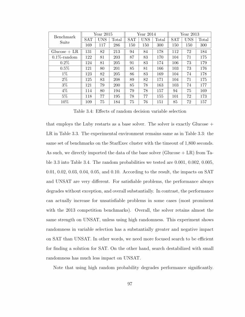
BenchmarkSuite

Year 2015 Year 2014 Year 2013SAT UNS Total SAT UNS Total SAT UNS Total169 117 286 150 150 300 150 150 300

Glucose + LR 131 82 213 94 84 178 112 72 184

0.1%-random 122 81 203 87 83 170 104 71 175

0.2% 124 81 205 91 83 174 106 73 179

0.5% 121 80 201 85 81 166 103 73 176

1% 123 82 205 86 83 169 104 74 178

2% 125 83 208 89 82 171 104 71 175

3% 121 79 200 85 78 163 103 74 177

4% 114 80 194 79 78 157 94 75 169

5% 118 77 195 78 77 155 101 72 173

10% 109 75 184 75 76 151 85 72 157

Table 3.4: Effects of random decision variable selection

that employs the Luby restarts as a base solver. The solver is exactly Glucose +

LR in Table 3.3. The experimental environment remains same as in Table 3.3: the

same set of benchmarks on the StarExec cluster with the timeout of 1,800 seconds.

As such, we directly imported the data of the base solver (Glucose + LR) from Ta-

ble 3.3 into Table 3.4. The random probabilities we tested are 0.001, 0.002, 0.005,

0.01, 0.02, 0.03, 0.04, 0.05, and 0.10. According to the result, the impacts on SAT

and UNSAT are very different. For satisfiable problems, the performance always

degrades without exception, and overall substantially. In contrast, the performance

can actually increase for unsatisfiable problems in some cases (most prominent

with the 2013 competition benchmarks). Overall, the solver retains almost the

same strength on UNSAT, unless using high randomness. This experiment shows

randomness in variable selection has a substantially greater and negative impact

on SAT than UNSAT. In other words, we need more focused search to be efficient

for finding a solution for SAT. On the other hand, search destabilized with small

randomness has much less impact on UNSAT.

Note that using high random probability degrades performance significantly.

97

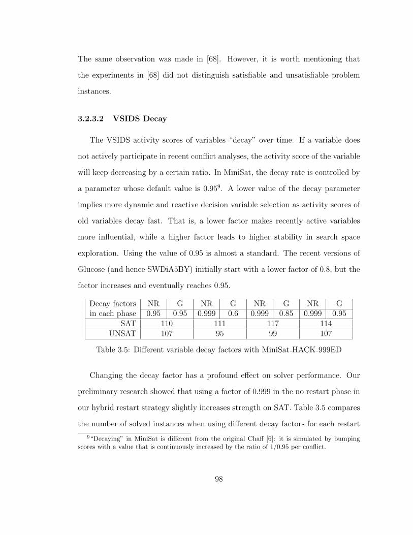
The same observation was made in [68]. However, it is worth mentioning that

the experiments in [68] did not distinguish satisfiable and unsatisfiable problem

instances.

3.2.3.2 VSIDS Decay

The VSIDS activity scores of variables “decay” over time. If a variable does

not actively participate in recent conflict analyses, the activity score of the variable

will keep decreasing by a certain ratio. In MiniSat, the decay rate is controlled by

a parameter whose default value is 0.959. A lower value of the decay parameter

implies more dynamic and reactive decision variable selection as activity scores of

old variables decay fast. That is, a lower factor makes recently active variables

more influential, while a higher factor leads to higher stability in search space

exploration. Using the value of 0.95 is almost a standard. The recent versions of

Glucose (and hence SWDiA5BY) initially start with a lower factor of 0.8, but the

factor increases and eventually reaches 0.95.

Decay factors NR G NR G NR G NR Gin each phase 0.95 0.95 0.999 0.6 0.999 0.85 0.999 0.95

SAT 110 111 117 114UNSAT 107 95 99 107

Table 3.5: Different variable decay factors with MiniSat HACK 999ED

Changing the decay factor has a profound effect on solver performance. Our

preliminary research showed that using a factor of 0.999 in the no restart phase in

our hybrid restart strategy slightly increases strength on SAT. Table 3.5 compares

the number of solved instances when using different decay factors for each restart

9“Decaying” in MiniSat is different from the original Chaff [6]: it is simulated by bumpingscores with a value that is continuously increased by the ratio of 1/0.95 per conflict.

98

phase. The benchmarks are from SAT Competition 2013. We used a timeout of

5,000 seconds on the machine configuration C. NR and G in the table refer to,

respectively, the no restart phase and the Glucose phase. The hybrid strategy was

implemented on top of MiniSat HACK 999ED. The first solver using the default

decay factor of 0.95 for both phases is the base solver that simply implements

the two alternating restart phases. The other three solvers switch decay factors

for respective phases (and thus disable Glucose’s feature of initially starting with

the value of 0.8). Note that we tested only 0.999 for the no restart phase. The

reason is that 0.999 was our first choice that showed immediate improvement in our

preliminary research. Unfortunately, having little computing resource, we could

not try other values for the no restart phase. From these observations, we decided

to use the factor of 0.999 in the no restart phase. For the Glucose phase, however,

we retained the default value of 0.95, since this value appears to be an optimal

value for the moment.

Ultimately, we implemented an elaborate approach of maintaining two separate

sets of VSIDS scores (hence two separate priority queues for variable selection),

each used exclusively for one restart phase. Our motivation was to reduce inter-

ference on VSIDS activity scores by the no-restart phases and the Glucose phases.

In detail, VSIDS scores in both sets are bumped and decayed together as usual in

each phase. However, the scores are decayed with different decay factors of 0.999

and 0.95 for each respective set. This scheme seems to give more robust outcomes

and work better than simply switching the decay factors (also better on the 2014

Competition benchmarks).

In fact, a very similar idea already appeared once in a solver in a past com-

petition. However, the idea was never documented, so one has to read the actual

99

source code of the solver to discover the idea. As mentioned before, the signature

feature of ZENN is the search diversification with a hybrid scheme. The author of

ZENN seemed to have tried many interesting hybridization ideas. One of the ideas

in the 2013 competition version of ZENN is to use different decay factors in a way

similar to ours. ZENN uses the decay factor of 0.99 for the phase with infrequent

restarts, and 0.8 for the phase with the Glucose-like restarts. However, the author

abandoned this idea in the new solver ROKK in the following year. Because there

exists no publication, it is not clear why the author decided to implement and later

abandon the idea. Like in the Luby case, it would be interesting to revisit this

idea in more depth.

SWD SWD+H SWD+H+3T LingelingGlucose

Core LBD cut 5 5 3 ayv aqw

SAT 109 129 133 122 119 1042013 UNSAT 123 126 132 107 112 112

Total 232 255 265 229 231 216

SAT 88 90 94 86 88 852011 UNSAT 104 101 102 94 93 108

Total 192 191 196 180 181 193

Table 3.6: No. solved instances with new hybrid techniques on 600 benchmarksfrom SAT Competition 2013 and 2011

The results of implementing the simple hybrid restart strategy (Section 3.2.2)

together with the alternating decay factors are already presented in Table 3.1 in

Section 3.2.1, in the columns under SWDiA5BY + Hybrid Strategy. Recall that we

tested 7 different core LBD limits (0 to 6) with the new solver. Since SWDiA5BY

uses the LBD limit of 5, it is best to compare the 5-LBD-limit version against

SWDiA5BY. For convenient reference, we present Table 3.6 here that duplicates

the data of Table 3.1 for these two solvers. In addition, we include the results

of other state-of-the-art solvers in the table for comparison. Lingeling ayv is the

100

winner in the application track in SAT Competition 2014, and Lingeling aqw is

the winner in SAT Competition 2013. SWD+H is the solver that implements

the hybrid restarts and alternating decay factors on top of SWDiA5BY (using

the LBD limit 5 as SWDiA5BY). SWD+H+3T is another version that we will

explain in a later section. With the 2013 competition benchmarks, we observe a

dramatic improvement of the hybrid strategy over SWDiA5BY for the satisfiable

instances. However, recall that there were 30 instances (001-010.cnf) for which the

Luby restarts were very effective compared to the Glucose restarts. Because of

these 30 instances, the table shows heavily biased results toward SWD+H. Indeed,

the dramatic improvement mostly comes from these instances (for all LBD limits).

Next, for the 2011 satisfiable instances, SWD+H also shows a slightly better result

(consistently for all core LBD limits). However, the degree of the improvement is

rather marginal with the short timeout. For the 2013 UNSAT instances, SWD+H

shows a slightly better result than SWDiA5BY, but this is not the case with the

2011 UNSAT. In fact, we report that the overall strength on UNSAT is slightly

reduced, particularly in terms of CPU time. This overhead on UNSAT is not really

a surprise, since the entire runtime is divided into two different restart phases.

Considering that only two thirds of the runtime is spent for the Glucose phase, this

slight degradation on UNSAT is actually encouraging. We succeeded in integrating

the strength of infrequent restarts on SAT while not sacrificing the strength on

UNSAT too much. Still, we conclude that this hybrid strategy is too primitive.

Our purpose was to prove that even this simple scheme can reliably bring the

benefits of infrequent restarts to complement the weakness of the Glucose restarts

on UNSAT. Moreover, when considering the relative performance of SWD+H with

other state-of-the-art solvers, our experiment also confirms that a hybrid approach

101

can be a very attractive option in modern solvers.

In the following section, we show one possible way of achieving further improve-

ment on both SAT and UNSAT by exploiting the insights we gained about learned

clauses with respect to SAT/UNSAT.

3.3 Refinement on Learned Clause Management

We have not yet presented a concrete method to exploit the different roles of

learned clauses between SAT and UNSAT. In this section, we refine the learned

clause management scheme of SWDiA5BY to exploit what we gained in Sec-

tion 3.2.1. We show that the new management scheme brings further improvement

on both SAT and UNSAT.

Table 3.1 (Section 3.2.1) showed that clauses of LBD >5 are barely useful in

a practical and global sense. For UNSAT, it is rather the low-LBD clauses that

play a central role of establishing a foundation that provides sufficient lemmas

necessary for constructing an UNSAT proof. It is for this reason that we used the

core LBD limit of 5 for our solver SWDiA5BY. However, we observed in Figure 3.4

that clauses with higher LBD can help reach an UNSAT proof “faster” in terms

of required conflicts. In this sense, giving a little bit more margin for clauses with

slightly higher but sufficiently low LBD may be advantageous to keep around for

a while. On the other hand, even LBD >1 does not seem to help much for SAT in

practice. There could be a compromise that works well for both SAT and UNSAT

in this context. We designed and tried an idea of adding a mid-tier in the clause

database, in addition to the existing two tiers for the core and local clauses. The

idea is to lower the core LBD limit so that a solver maintains a more compact

102

database mainly for SAT, while the mid-tier accommodates recently used clauses

of higher LBD between 4 and 6 for UNSAT. The mid-tier functions as a buffer

and staging area in that clauses may stay as long as but only if they have been

involved in recent conflict analyses. The mid-tier is checked for reduction at every

10,000 conflicts, and clauses not used in the past 30,000 conflicts are demoted to

the local tier. There are still a few subtleties in the actual implementation details,

but this concept of the mid-tier is the essence of the refinement. To recapitulate,

(1) we bring down the core LBD limit to 3 for increased efficiency on SAT; while

(2) we retain recently used clauses of LBD up to 6 in addition to local clauses in

the hope that those mid-tier clauses can be used efficiently as bridging elements for

an UNSAT proof. We implemented this idea on top of SWDiA5BY that already

implements our hybrid strategy. The performance result is presented in Table 3.6

under the column SWD+H+3T. We can see substantial improvement both on SAT

and UNSAT with the 2013 competition benchmarks. We also see improvements

with the 2011 benchmarks, although the degree of the improvement is smaller with

the short timeout.

In fact, this idea of keeping clauses that were involved in recent conflicts in

the mid-tier was inspired by ROKK [91]. ROKK showed remarkable performance

in SAT Competition 2014 (7th in the SAT+UNSAT track and 6th in the SAT

track). The solver uses a hybrid strategy, and its learned clause management is

very peculiar. Basically, the solver reduces the database at every 10,000 conflicts

(i.e., high tendency towards shrinking to 5,000 clauses over time), while protecting

recently used clauses in a similar (but much more complex) way to our mid-tier

clauses.

An interesting observation is the completely different characteristics that this

103

mid-tier exhibited in each restart phase. For the no-restart phase, the size of the

tier decreases quickly over time. Literals per learned clause (in an overall sense)

tend to increase quickly too. The general implication is that, when remaining in the

current search space without restarts, new learned clauses are used mostly locally

and thus rarely get reused. However, the situation is opposite in the Glucose-style

restart phase in general, although the size of the tier does not grow much anyway

due to the low limit of 30,000 conflicts to be considered recent.

3.4 Concluding Remarks

There exist many ways to improve performance on SAT while having negative

impact on UNSAT (and vice versa). There exists an unfortunate trade-off between

SAT and UNSAT. (Similar arguments about these two opposing forces also appear

in [29].) It is relatively easy to improve performance only on either SAT or UNSAT

if we are willing to sacrifice the strength on the other. In practice, we can imme-

diately benefit from this fact by running two SAT- and UNSAT-specialized solvers

in parallel. On the other hand, improving performance on SAT and UNSAT at the

same time is not an easy task. However, as shown in this chapter, understanding

and carefully exploiting the SAT/UNSAT difference can achieve improvement on

both SAT and UNSAT. Indeed, this claim is supported strongly by the results of

the SAT-Race 2015 where we submitted two solvers implementing the techniques

described in this chapter.

We also emphasize that the hybrid strategy presented in this chapter is very

primitive. We designed the strategy to be as simple as possible only to highlight

and explain the varying degree of effects on SAT and UNSAT with respect to the

104

frequency of restarts. Due to resource and time constraints, we were not able

to conceive and test more sophisticated methods. Moreover, we believe that the

current state of the presented strategy is far from maintaining an optimal balance

between SAT and UNSAT. There may exist largely different ways that better

exploit the SAT/UNSAT difference than the ways presented here. We also want

to make a note that revisiting previous research with the difference in mind may

shed more light on the internal workings of CDCL.

Lastly, we emphasize that all the arguments in this paper apply only to prob-

lems from the industrial domain. Particularly, it may not work as explained for

the hand-crafted combinatorial problems. It is well-known that industrial problems

are very different from hand-crafted ones although they share some similarities. It

will be interesting to find out in which ways they are different, which might give

new insights on the CDCL workings. Similarly, the structure of one benchmark

series can be very different from the structure of another. One strategy cannot be

universally good for every series.

105

Chapter 4

COMiniSatPS

In this chapter, we present a reference solver COMiniSatPS1 that implements

all the techniques described in this thesis. The solver is an official successor of

our award-winning SWDiA5BY. As explained, SWDiA5BY implements on top of

Glucose a simple idea of core and local clauses described in Chapter 2. COMin-

iSatPS then implements the ideas presented in Chapter 3 on top of SWDiA5BY.

Because Glucose is a MiniSat derivative, COMiniSatPS can also be considered as

a MiniSat and Glucose derivative. However, we built COMiniSatPS fresh on top

of MiniSat instead of on top of SWDiA5BY or Glucose. The intention is to retain

the minimalist spirit of the critically acclaimed MiniSat. The purposes of building

COMiniSatPS and presenting the work in this thesis are multi-fold:

1. Manifestation of concrete improvement of the state of the art

of CDCL. Our focus is on improving the CDCL framework itself. Note

that, according to [76], the four major components of CDCL solvers are

Conflict-Driven Clause Learning [4], activity-based variable branching heuris-

1Source is available at http://www.cs.nyu.edu/~chanseok/cominisatps/.

106

tics [6], Boolean Constraint Propagation using lazy data structures [6], and

restarts [19]. Additionally, since Glucose [3], aggressive clause removal poli-

cies are essential ingredients of CDCL solvers [16]. Our solver COMiniSatPS

has a focus on making changes only to the above five major elements of

CDCL. Note that innovations and improvements on these five major ele-

ments in CDCL have been stagnating recently. For example, since 2012,

the official releases of Glucose have not seen any changes except for minor

enhancements, in the context of sequential SAT solving. Our perspective is

that Glucose represents the current standard of CDCL well to some extent.

The basis for our perspective is that, e.g., the majority of the solver par-

ticipants in SAT-Race 2015 are based on Glucose, use Glucose directly as

a core sub-component, or at least implement all the strategies of Glucose.

In fact, our solver COMiniSatPS does not implement any other techniques

(besides our own techniques) beyond what Glucose currently provides. Past

SAT competitive events have already shown the large degree of performance

improvement of our solvers (SWDiA5BY and COMiniSatPS) over Glucose.

This result of concrete improvement effectively suggests a potential advance-

ment of the current standard of CDCL. More importantly, this manifestation

suggests that there is still room for improvement inside CDCL.

2. Manifestation that a simple CDCL framework alone can be as per-

formant as any state-of-the-art SAT solvers. The stagnation of inno-

vations inside CDCL might be partially responsible for the diverse and or-

thogonal nature of a wide spectrum of recent research work that is external

to CDCL. (In our scope, formula simplification such as preprocessing [43] or

inprocessing [21] is external to CDCL, unless such a simplification technique

107

is simple, effective, and necessary to become an integral part of CDCL.) The

highly complex nature of recent work has spawned many state-of-the-art SAT

solvers with complex implementations outside CDCL. However, interestingly,

past competitions have shown that our solvers with a simple CDCL frame-

work are at least as performant as any such state-of-the-art SAT solver. Not

only do these results prove the effectiveness of our new techniques but they

do suggest that state-of-the-art solvers are now showing largely saturated

performance.

3. Providing a base solver with a new level of performance to foster

practical SAT research. A technique shown to be effective on one solver

often may not be efficient when implemented in another solver. For exam-

ple, [68] reported that conflict clause minimization [107] can significantly

improve the conflict analysis. However, the same thesis reported that when

the conflict clause minimization is used, all other suggested improvements

for conflict analysis do not improve the performance significantly. As shown

in this example, new techniques that achieve the next level of performance

can subsume or nullify the efficiency of other techniques. The performance

of the popular MiniSat solver falls far behind modern solvers (Table 3.3).

In fact, MiniSat is no longer developed or maintained since the last 2.2.0

version that was released several years ago. However, due to the virtues of

minimality, simplicity, and fairly good performance of MiniSat, researchers

still choose MiniSat as a base solver for analyzing and evaluating various

aspects of CDCL (e.g., in [80, 77, 112]). However, because the state-of-the-

art solvers employ radically different strategies especially for restarts and

clause management, it is very possible that techniques shown to be effec-

108

tive in MiniSat may have no impact when implemented in a state-of-the-art

solver. We try to remedy this problem by providing a simple reference solver

that delivers state-of-the-art performance. The ultimate goal is to expedite

the advancements in practical SAT research by promoting our solver as a

new and right platform of choice. To achieve this goal, we follow the same

minimalistic spirit of MiniSat. We apply only minimally necessary changes

to MiniSat to make the solver efficient. As a result, COMiniSatPS is a very

compact implementation of the CDCL framework as in MiniSat.

4. Wide and rapid dissemination of the essential and effective tech-

niques to bring the new level of performance. One important goal

of COMiniSatPS is to provide the implementations for the new techniques

in a highly accessible and digestible form. To achieve the goal, we choose

the last available version (2.2.0) of MiniSat as a base solver and implement

the necessary techniques in small incremental steps. The actual form of the

incremental implementation is a series of small diff patches. Each patch im-

plements a particular feature, one at a time. Applying all the patches will

produce the final form of COMiniSatPS. However, each patch also results in

a fully functional solver. We also craft the patches in a careful way to mini-

mize the effort required to understand the necessary changes. We eliminate

any unnecessary clutter and minimize the code size in diff. Implementations

explained in the diff form are easy to understand and thus benefit a wide

audience, particularly starters and non-specialists in practical SAT. This diff

form will also make it easy for researchers to adopt and implement the tech-

niques in their own solvers in a correct way.

109

5. Describing other techniques not covered in the previous chapters.

The actual COMiniSatPS version that achieved an impressive result in the

recent SAT-Race 2015 implements some techniques that have not been de-

scribed in the previous chapters. We did not describe these techniques pre-

viously as they do not have strong relevance to the topics or they are not

major enhancements. However, these techniques are important in that they

are required to achieve the observed performance in the competition.

6. Fine-grained evaluation of performance impact of each of the new

techniques. Recall that each patch results in a fully functional solver. This

property of the patches make it easy to evaluate how much each individual

patch contributes to the solver performance. In the later part of this chapter,

we evaluate and report the individual performance impact of each of the

techniques in an incremental fashion.

4.1 Introduction

In [26], we made an observation that very simple solvers with tiny but critical

changes (e.g., MiniSat hack solvers) can be impressively competitive or even out-

perform complex state-of-the-art solvers. However, the original MiniSat itself is

vastly inferior to modern SAT solvers in terms of actual performance. This is no

wonder as it has been several years since the last 2.2.0 release of MiniSat. To match

the performance of modern solvers, MiniSat needs to be modified to add some of

highly effective techniques discovered recently. Fortunately, small modifications

are enough to bring up the performance of any simple solver to the performance

level of modern solvers. COMiniSatPS adopts only simple but truly effective ideas

110

that can make MiniSat competitive with recent state-of-the-art solvers. In the

same minimalistic spirit of MiniSat, COMiniSatPS prefers simplicity over com-

plexity to reach out to a wide audience. As such, the solver is provided as a series

of incremental patches to the original MiniSat. Each small patch adds or enhances

one feature at a time and produces a fully functional solver. Each patch often

changes solver characteristics fundamentally. This form of source distribution by

patches would benefit a wide range of communities as it is easy to isolate, study,

implement, and adopt the ideas behind each incremental change. The goal of CO-

MiniSatPS is to lower the entering bar so that anyone interested can implement

and test their new ideas easily on a simple solver guaranteed to have exceptional

performance.

4.2 Patch Descriptions

The first Patch 01 effectively turns MiniSat into Glucose 2.3 that participated

in SAT Competitions 2013 and 2014. To prove that the patch implements all

the techniques of Glucose properly and efficiently, we crafted Patch 01 in a way

that the resulting solver after applying the patch perfectly simulates the same

logical execution2 of Glucose 2.3. The next Patch 02 subsequently turns the solver

into SWDiA5BY (version A26) that participated in SAT Competition 2014. The

resulting solver again perfectly simulates the same logical execution of SWDiA5BY.

The Patch 01 is physically a single diff patch file. However, we divided the

Patch 01 into two parts below to better explain the changes in the patch. The

2We are referring to the logical equivalence in execution, modulo physical properties. Forexample, memory consumption, garbage collection frequency, and output messages will differ.However, it is not impossible that the logical equivalence may become broken in certain rarecases of, e.g., arithmetic overflow.

111

intention is to highlight the logical separation of the two parts. We also divided

Patch 06 into two parts so that we can conveniently refer to each part when we

report the performance evaluation of each part later.

1. Patch 01 (Part 1). The first part of the patch implements the essence of

Glucose, i.e., the two signature features of Glucose: 1) the LBD-based rapid

restarts with blocking restarts [29]; and 2) the LBD-based learned clause

management [3]. In addition, the patch implements the following three small

enhancements or optimizations in Glucose: 1) the dynamic LBD update [3];

2) the slowly increasing variable decay factor in the early stage of search [56];

and 3) the extra bumping of VSIDS activity scores of certain variables in a

newly generated learned clause [3]. The patch also disables preprocessing if

the number of clauses of an input CNF formula is greater than 4,800,000.

This change in preprocessing is to make a resulting solver run in exactly

the same way as the Glucose version (2.3) submitted to SAT Competitions

2013 and 2014. For the same reason, the patch does not fix benign bugs in

Glucose such as imprecise computation of runtime statistics. The patch also

adds some minor technical and mechanical optimizations.

2. Patch 01 (Part 2). If the Part 1 implemented the essence of Glucose,

Part 2 can be seen as an additional optimization. This part of the patch

implements 1) the dedicated watch lists [6] for binary clauses; and 2) the

limited self-subsuming simplification of certain learned clauses using binary

resolution [54]. These two techniques are part of the original Glucose. After

applying this patch, the resulting solver perfectly simulates Glucose 2.3.

3. Patch 02. This patch implements the notion of core and local clauses de-

112

scribed in Chapter 2. In fact, this patch effectively turns the previous solver

into SWDiA5BY. As in SWDiA5BY, this patch fixes the LBD computation

bug of the original Glucose in which the decision level 0 is counted towards

LBD computation when dynamically updating the LBD. After applying this

patch, the resulting solver perfectly simulates the execution of SWDiA5BY.

4. Patch 03. This patch applies a few minor enhancements and tiny technical

fixes. As such, this patch could have been merged into the next Patch 04. We

factored out these minor changes into the Patch 03 so that everything inside

Patch 04 is only about implementing the 3-tiered clause management scheme

(Chapter 3). One enhancement in this patch is still worth documenting. If

the LBD of a learned clause is greater than 50, the solver treats such a

clause as if its LBD is 50 when computing the global LBD average. By this

technique, the global LBD average can be lower than the actual average if

solvers learn many clauses whose LBD is greater than 50. We discovered that

for some problem instances, the actual global LBD average is initially very

high (e.g., over 200) when we employ a hybrid restart strategy (Chapter 3).

Recall that the global LBD average is used for triggering restarts. A high

global average implies that the solver will tolerate generating many high-LBD

clauses by not initiating restarts often. By forcing a lower global average, we

trick the solver into thinking that it is learning clauses with unusually high

LBD values. As a result, the solver will trigger restarts as rapid as possible

if the gap between the actual average and the lowered average is huge. We

discovered that rapid restarts help tremendously for certain problems with

a high initial LBD average. For such problem instances, this technique also

brings down the global average much more quickly. However, we make a note

113

that this technique is not universally effective on every problem instance.

5. Patch 04. This patch implements the 3-tiered learned clause management

scheme described in Chapter 3. Clauses in the 3rd tier (local clauses) can

be promoted to the 2nd tier (mid-tier clauses) if the LBD is updated to fall

in the range of 4 to 6. Similarly, mid-tier clauses can be demoted to the

local tier if the clauses have not been touched in the past 30,000 conflict

analysis. The solver checks the mid-tier at every 10,000 conflicts to demote

such clauses. Note that it is unnecessary to maintain activity scores for the

mid-tier clauses because we only check if the clauses are involved in recent

conflicts. Therefore, we do not increase the activity scores of the mid-tier

clauses even if they are involved in conflict analysis. In this way, we also

prevent the solver from triggering unnecessary rescaling of the activity scores

of all variables when increasing a score induces (logical) overflow. When

demoting a mid-tier clause to the local tier, the solver sets the activity score

of the clauses to 0. The rationale for the reset is to be consistent with the

fact that new (local) learned clauses are initialized with the activity score of

0. Because the solver will constantly demote a lot of mid-tier clauses to the

local tier, this patch also changes the way the local tier is reduced. Recall

that SWDiA5BY removes (roughly) the half of the local clauses whenever

the size of the local tier reaches the hard limit of 20,000. To accommodate

the additional clauses flowing from the mid-tier into the local tier, this patch

attempts to slightly increase the hard limit for the local clauses. Specifically,

the first database reduction of the local tier happens at 30,000 conflicts.

Afterwards, the solver reduces the local tier at every 15,000 conflicts. Finally,

another technique included in this patch is to increase the core LBD limit

114

to 5 (3 is the default) if the solver learns fewer than 100 core clauses after

100,000 conflicts. This situation of learning fewer than 100 core clauses is

very rare in practice. However, we observed that there was one benchmark

series where this can happen. Increasing the core LBD limit may mitigate

potential problems arising from failing to accumulate low-LBD clauses.

6. Patch 05. This patch implements the hybrid restart strategy described in

Chapter 3. When computing the global LBD average, we only use those

clauses that are learned in the Glucose-restart phase. This is because the

clauses learned in the no-restart phase show radically different characteristics.

One additional enhancement included in this patch is to let the solver run in

the Glucose-restart phase for the first 10,000 conflicts. The hybrid strategy

then starts its normal cycle after the 10,000 conflicts. The intention is to

stabilize the solver in the early stages of search to compute a more accurate

global LBD average to begin with. We observed that the global LBD average

sometimes begins with an unusually high average if we start the hybrid cycles

right away. Lastly, we increase the sensitivity of initiating a restart in the

Glucose-restart phase when the phase runs over its allowed length of period.

To increase the sensitivity, we increase the ‘K’ value [29] from 0.8 to 0.9

temporarily if the Glucose phase is prolonged.

7. Patch 06 (Part 1). This patch uses the alternating variable decay factors

(Chapter 3), each set and used in the respective restart phase of the hybrid

restart strategy. This patch amounts to a few lines only as we merely switch

the decay factor values between 0.999 and 0.95. We also remove the feature

of the increasing decay factor [56] implemented in Glucose. For now, we have

115

not found a good way to retain the removed feature while we alternate the

two decay factors.

8. Patch 06 (Part 2). This patch implements the two separate priority vari-

able queues for decision variable selection (Chapter 3). The queues are used

to order variables according to the VSIDS variable activity scores. One queue

is used exclusively for variable selection in the no-restart phase. The other

queue is for the Glucose-restart phase. The intention in using the two sepa-

rate queues is to reduce the interference of the two orthogonal restart phases.

9. Patch 07. This optional patch optimizes the core data structure for storing

clauses to use less memory. Because the solver has to additionally record

the information of when each mid-tier clause is touched in the last conflict

analysis, COMiniSatPS increases the memory usage for clauses compared

to SWDiA5BY. We wanted to show through this patch that further low-

level optimization is possible to use much less memory. However, the patch

slightly increases the complexity of the low-level implementation, which is

against the overall philosophy of COMiniSatPS. The resulting solver after

this patch is very close to the COMiniSatPS version submitted to SAT-Race

2015.

10. Patch 08. This optional patch fixes a few minor bugs. Basically, this patch

is only for documentation purposes. Fixing the bugs has negligible effect on

actual performance. Some of the bugs are present in the original MiniSat.

One bug present in original MiniSat affects the correctness of the solver,

although the bug is not triggered when the default parameters are used.

11. Patch 09. This patch implements Incrementally Relaxed Bounded Variable

116

Elimination3 [108] that was originally proposed in the solver GlueMiniSat

2015 [108]. Unlike other patches, this patch changes the preprocessing step.

The implementation of the basic framework is very small and almost identical

to the implementation of GlueMiniSat. However, our policy is less lenient in

relaxing the tolerance bound of variable elimination.

4.3 Experimental Evaluation

In this section, we evaluate and verify the individual performance contribution

of each of the new techniques in COMiniSatPS.

BenchmarkSuite

Year 2015 Year 2014 Year 2013SAT UNS Total SAT UNS Total SAT UNS Total169 117 286 150 150 300 150 150 300

Glucose 127 95 222 91 101 192 95 87 182

Patch 01 127 95 222 91 101 192 95 87 182

Patch 02 127 95 222 94 100 194 98 89 187

Patch 04 132 97 229 94 102 196 98 90 188

Patch 05 137 96 233 95 100 195 102 86 188

Patch 06-1 140 95 235 96 100 196 107 87 194

Patch 06-2 138 96 234 96 100 196 116 90 206

Patch 07 138 96 234 96 101 197 116 90 206

Patch 09 140 98 238 98 103 201 115 90 205

Table 4.1: Performance comparison of solvers at different stages of patch applica-tion

Table 4.1 reports the performance of the solvers produced at different stages

of patch application. We used the StarExec cluster with a timeout of 1,800 sec-

onds. In fact, the execution environment and the benchmarks used are identical

3The authors of GlueMiniSat call the technique Incremental Variable Elimination. However,because we use the term ‘Incremental Variable Elimination’ to refer to the technique to enableBounded Variable Elimination [44, 43] in the context of incremental SAT, we prefer calling itIncrementally Relaxed Bounded Variable Elimination.

117

to those of Table 2.1, Table 2.2, Table 3.3, and Table 3.4. The third row reports

the performance of original Glucose4. For convenient reference, we briefly repeat

here what each patch implements. The fourth row (Patch 01) is a solver that

perfectly simulates original Glucose in the third row. The fifth row (Patch 02) is a

solver that simulates SWDiA5BY. Patch 04 implements the 3-tier learned clauses

management. Patch 05 implements the hybrid restart strategy. Patch 06-1 uses

the alternating variable decay factors. Patch 06-2 implements the two separate

variable priority queues. Patch 07 optimizes the solver to use less memory. Patch

09 implements the Incrementally Relaxed Bounded Variable Elimination.

First, we observe that the performance improvement of the final form of CO-

MiniSatPS over the original Glucose solver is consistently substantial across all

the benchmark suites. It is also generally true that the performance gradually

improves as we apply more patches. However, we caution the reader to not ex-

clude the possibility that our solver is highly tuned to the benchmarks used in the

experiment. Because the annual competitions reuse many benchmark instances

used in the previous years, there may also exist a certain bias towards the bench-

marks common to all the benchmark suites. Another point worth noting is that

the degree of improvement on the 2014 benchmark suite is much smaller than on

the other two benchmark suites. We can also see that, although our techniques do

improve performance on unsatisfiable problems, the techniques are still less effec-

tive on those problems. Recall that the original Glucose is already very strong on

4Alert readers might notice that the numbers for the original Glucose in this table are differentfrom those in Table 2.1 even though we used the exact same execution environment. Here in thisexperiment, we reran Glucose again together with the other solvers generated by the patches. Wedecided to reran it after noticing that the Patch 01 (which perfectly simulates original Glucose)gave strictly better results than Glucose. It is not clear why Glucose in this later experiment gaveimproved performance compared to the performance reported in Table 2.1. The experiment inthis chapter was performed some time later than the earlier experiments in the previous chapters.We suspect that the overall performance of the StarExec cluster has improved during the period.

118

unsatisfiable instances as we observed in Chapter 3.

119

Conclusion

There is no argument that the most important feature of a SAT solver is its

efficiency. Therefore, the majority of the research work done in the SAT commu-

nity is about improving the speed of SAT solvers [10]. As one of such works, this

thesis improves the state of the art of DPLL by exploiting empirical characteristics

exhibited by the current state of SAT solvers on real-world problems. The the-

sis solely focuses on the core DPLL structure where concrete advancements have

been stagnating recently. The thesis shows that old solvers with only the simple

DPLL structure can be rectified with small changes to achieve competitive perfor-

mance with any state-of-the-art solvers that implement complex features outside

DPLL. This result effectively proposes a new standard for DPLL and proves that

the current state of DPLL is not mature. Particularly, this thesis achieves the

improvement on the state of the art with fresh and unconventional approaches,

which subsequently provide new insights on the empirical characteristics of SAT

solvers in the modern settings.

First, this thesis presents and advocates an unconventional perspective on the

clauses that CDCL learns when working on real-world problems. Specifically, the

thesis provides data and analysis showing that the majority of the clauses learned

by CDCL are not useful for deriving a proof of unsatisfiability in terms of actual

solver performance in general. In addition, the thesis shows that an unconven-

tionally small fraction of clauses with certain quality is enough to solve real-world

problems fast in practice. This observation leads to the hypothesis that current

CDCL solvers are severely limited in that they are incapable of efficiently deriving

a sophisticated proof of unsatisfiability, or that the only problems CDCL solvers

can tackle efficiently are those problems that have a short proof that can be easily

120

constructed out of simple clauses.

Next, this thesis shows that CDCL works very differently when searching for

a satisfying solution and when deriving an unsatisfiability proof. Ultimately, the

thesis improves solver performance by exploiting the observed differences of CDCL.

The thesis gives partial explanations to the differences in terms of the workings

of some of the most important elements in CDCL: the effects of search restarts

and the branching heuristic, and the roles of learned clauses. The thesis provides

a wide range of concrete evidence and detailed analysis that highlight the varying

effects and roles of these elements between the satisfiable SAT problem case and

the unsatisfiable case. As a result, the thesis also sheds new light on the internal

workings of CDCL. With this better understanding of CDCL highlighted by the

differences between satisfiable and unsatisfiable cases, the thesis realizes substantial

performance improvements by making fundamental changes to various elements in

CDCL.

Lastly, this thesis presents a new solver COMiniSatPS developed as a proof

of concept for the techniques described throughout the thesis. The performance

improvement brought by COMiniSatPS over the state of the art when limited to

CDCL is substantial and is achieved by simple changes to the core elements of

CDCL. Therefore, in another sense, COMiniSatPS proposes a new state-of-the-art

standard for CDCL and serves as a reference implementation containing only mini-

mal and truly effective elements. This set of changes can turn old solvers with only

the simple CDCL framework into solvers whose performance is competitive with

any modern SAT solver. More importantly, the solver implementation is provided

in an unusual but highly digestible form: a series of diff patches against MiniSat.

This form of source distribution is chosen deliberately with the specific goal of

121

promoting COMiniSatPS to be a useful platform of choice for SAT researchers.

122

Bibliography

[1] Sorensson, N., and Een, N. Minisat 2.1 and Minisat++ 1.0 — SAT Race 2008

Editions. SAT 2009 Competitive Events Booklet: Preliminary Version (2009).

[2] Een, N., and Sorensson, N. An Extensible SAT-solver. Theory and Applica-

tions of Satisfiability Testing (2004).

[3] Audemard, G., and Simon, L. Predicting Learnt Clauses Quality in Modern

SAT Solvers. IJCAI (2009).

[4] Marques-Silva, J., and Sakallah, K. GRASP—A New Search Algorithm for

Satisfiability. Proceedings of the 1996 IEEE/ACM International Conference

on Computer-aided Design (1997).

[5] Marques-Silva, J., and Sakallah, K. GRASP: A Search Algorithm for Propo-

sitional Satisfiability. IEEE Transactions on Computers (1999).

[6] Moskewicz, M., Madigan, C., Zhao, Y., Zhang, L., and Malik, S. Chaff: En-

gineering an Efficient SAT Solver. Proceedings of the 38th Annual Design Au-

tomation Conference (2001).

[7] Bryant, R. Graph-Based Algorithms for Boolean Function Manipulation.

IEEE Transactions on Computers (1986).

123

[8] Selman, B., Kautz, H., and Cohen, B. Local Search Strategies for Satisfiability

Testing. Cliques, Coloring, and Satisfiability: Second DIMACS Implementa-

tion Challenge (1993).

[9] Cook, S. The Complexity of Theorem-proving Procedures. Proceedings of the

Third Annual ACM Symposium on Theory of Computing (1971).

[10] Zhang, L. Searching for Truth: Techniques for Satisfiability of Boolean For-

mulas. PhD thesis, Princeton University (2003).

[11] Davis, P., and Putnam, H. A Computing Procedure for Quantification Theory.

Journal of the ACM (1960).

[12] Davis, P., Logemann, G., and Loveland, D. A Machine Program for Theorem

Proving. Communications of the ACM (1962).

[13] Ansotegui, C., Giraldez-Cru, J., and Levy, J. The Community Structure of

SAT Formulas. Theory and Applications of Satisfiability Testing (2012).

[14] Newsham, Z., Ganesh, V., Fischmeister, S., Audemard, G., and Simon, L.

Impact of Community Structure on SAT Solver Performance. Theory and

Applications of Satisfiability Testing (2014).

[15] Ganian, R., and Szeider, S. Community Structure Inspired Algorithms for

SAT and #SAT. Theory and Applications of Satisfiability Testing (2015).

[16] Ansotegui, C., Giraldez-Cru, J., Levy, J., and Simon, L. Using Community

Structure to Detect Relevant Learnt Clauses. Theory and Applications of Sat-

isfiability Testing (2015).

124

[17] Aloul, F., Sakallah, K., and Markov, I. Efficient Symmetry Breaking for

Boolean Satisfiability. IEEE Transactions on Computers (2006).

[18] Devriendt, J., Bogaerts, B., and Bruynooghe, M. BreakIDGlucose: On the

Importance of Row Symmetry in SAT. Proceedings of the 4th International

Workshop on the Cross-Fertilization Between CSP and SAT (2014).

[19] Gomes, C., Selman, B., and Kautz, H. Boosting Combinatorial Search

Through Randomization. AAAI/IAAI (1998).

[20] Gomes, C., Selman, B., and Crato, N. Heavy-tailed Distributions in Combi-

natorial Search. Principles and Practice of Constraint Programming (1997).

[21] Jarvisalo, M., Heule, M., and Biere, A. Inprocessing Rules. Automated Rea-

soning (2012).

[22] Haken, A. The Intractability of Resolution. Theoretical Computer Science

(1985).

[23] Pipatsrisawat, K., and Darwiche, A. On the Power of Clause-Learning SAT

Solvers as Resolution Engines. Artificial Intelligence (2011).

[24] Urquhart, A. Hard Examples of Resolution. Journal of the ACM (1987).

[25] Chvatal, V., and Szemerdi, E. Many Hard Examples of Resolution. Journal

of the ACM (1988).

[26] Oh, C. Between SAT and UNSAT: The Fundamental Difference in CDCL

SAT. Theory and Applications of Satisfiability Testing (2015).

[27] Oh, C. Patching MiniSat to Deliver Performance of Modern SAT Solvers.

SAT-Race (2015).

125

[28] Biere, A., Cimatti, A., Clarke, E., and Zhu, Y. Symbolic Model Checking

without BDDs. Tools and Algorithms for the Construction and Analysis of

Systems (1999).

[29] Audemard, G., and Simon, L. Refining Restarts Strategies for SAT and UN-

SAT. Principles and Practice of Constraint Programming (2012).

[30] Biere, A., Heule, M., Van Maaren, H., and Walsh, T. Handbook of Satisfiability

(2009).

[31] Enderton, H. A Mathematical Introduction to Logic. (2001).

[32] Hadarean, L. An Efficient and Trustworthy Theory Solver for Bit-vectors in

Satisfiability Modulo Theories. PhD thesis, New York University (2014).

[33] Tseitin, G. On the Complexity of Derivation in Propositional Calculus. Struc-

tures in Constructive Mathematics and Mathematical Logic, Part II, Seminars

in Mathematics (1968).

[34] Jackson, P., and Sheridan, D. Clause Form Conversions for Boolean Circuits.

Theory and Applications of Satisfiability Testing (2004).

[35] Plaisted, D., and Greenbaum, S. A Structure-preserving Clause Form Trans-

lation. Journal of Symbolic Computation (1986).

[36] Zabih, R., and McAllester, D. A Rearrangement Search Strategy for Deter-

mining Propositional Satisfability. Proceedings of the National Conference on

Artificial Intelligence (1988).

[37] Robinson, J. A Machine-Oriented Logic Based on the Resolution Principle.

Journal of the ACM (1965).

126

[38] Robinson, J. Logic: Form and Function: The Mechanization of Deductive

Reasoning. (1979).

[39] Heule, M., and Biere, A. Proofs for Satisfiability Problems. All about Proofs,

Proofs for all (2015).

[40] Ben-Sasson, E., and Wigderson, A. Short Proofs are Narrow — Resolution

made Simple. Proceedings of the Thirty-first Annual ACM Symposium on The-

ory of Computing (1999).

[41] Wang, H. MINIPURE. SAT Competition (2013).

[42] Ryan, L. Efficient Algorithms for Clause-learning SAT Solvers. PhD thesis,

Simon Fraser University (2004).

[43] Een, N., and Biere, A. Effective Preprocessing in SAT Through Variable and

Clause Elimination. Theory and Applications of Satisfiability Testing (2005).

[44] Subbarayan, S., and Pradhan, D. NiVER: Non-increasing Variable Elimina-

tion Resolution for Preprocessing SAT instances. Theory and Applications of

Satisfiability Testing (2004).

[45] Bjork, M. Successful SAT Encodings Techniques. Journal on Satisfiability,

Boolean Modeling and Computation (2009).

[46] Zhang, L., Madigan, C., Moskewicz, M., and Malik, S. Efficient Conflict

Driven Learning in a Boolean Satisfiability Solver. Proceedings of the 2001

IEEE/ACM international conference on Computer-aided design (2001).

127

[47] Dershowitz, N., Hanna, Z., and Nadel, A. Towards a Better Understanding of

the Functionality of a Conflict-Driven SAT Solver. Theory and Applications

of Satisfiability Testing (2007).

[48] Biere, A., and Fohlich, A. Evaluating CDCL Variable Scoring Schemes. Theory

and Applications of Satisfiability Testing (2015).

[49] Biere, A. Adaptive Restart Strategies for Conflict Driven SAT Solvers. Theory

and Applications of Satisfiability Testing (2008).

[50] Luby, M., Sinclair, A., and Zuckerman, D. Optimal Speedup of Las Vegas

Algorithms. Israel Symposium on Theory of Computing Systems (1993).

[51] Pipatsrisawat, K., and Darwiche, A. A Lightweight Component Caching

Scheme for Satisfiability Solvers. Theory and Applications of Satisfiability

Testing (2007).

[52] Audemard, G., and Simon, L. Lazy Clause Exchange Policy for Parallel SAT

Solvers. Theory and Applications of Satisfiability Testing (2014).

[53] Ryvchin, V., and Strichman, O. Local Restarts in SAT. Theory and Applica-

tions of Satisfiability Testing (2008).

[54] Audemard, G., and Simon, L. GLUCOSE 2.1 in the SAT Challenge 2012.

SAT Challenge (2012).

[55] Audemard, G., and Simon, L. GLUCOSE 2.1 Aggressive — but Reactive —

Clause Database Management, Dynamic Restarts. Pragmatics of SAT (2012).

[56] Audemard, G., and Simon, L. GLUCOSE 2.3 in the SAT 2013 Competition.

SAT Competition (2013).

128

[57] Audemard, G., and Simon, L. Glucose 3.1 in the SAT 2014 Competition. SAT

Competition (2014).

[58] Li, C., Xiao, F., and Ruchu Xu, R. Glucose nbSat and Glucose nbSatRsltn.

SAT-Race (2015).

[59] Walsh, T. Search in a Small World. IJCAI (1999).

[60] Goldberg, E., and Novikov, Y. BerkMin: A Fast and Robust Sat-solver. Dis-

crete Applied Mathematics (2007).

[61] Nadel, A., Gordon, M., Palti, A., and Hana, Z. Eureka-2006 SAT solver.

SAT-Race (2006).

[62] Biere, A. PicoSAT Essentials. Journal on Satisfiability, Boolean Modeling and

Computation (2008).

[63] Biere, A. P{re,i}coSAT@SC09. SAT Competition (2009).

[64] Huang, J. The Effect of Restarts on the Efficiency of Clause Learning. IJCAI

(2007).

[65] Pipatsrisawat, K., and Darwiche, A. RSat Description for SAT Competition

2009. SAT Competition (2009).

[66] Pipatsrisawat, K., and Darwiche, A. RSat 2.0: SAT Solver Description. SAT

Competition (2007).

[67] Huang, J. A Case for Simple SAT Solvers. Principles and Practice of Con-

straint Programming (2007).

129

[68] Manthey, N. Improving SAT Solvers Using State-of-the-Art Techniques. PhD

thesis, Technische Universitat Dresden (2010).

[69] Kahlert, L., Kruger, F., Manthey N., and Stephan A. Riss Solver Framework

v5.05. SAT-Race (2015).

[70] Soos, M., and Lindauer, M. The CryptoMiniSat-4.4 set of solvers at the SAT

Race 2015. SAT-Race (2015).

[71] Claessen, K., Een, N., Sheeran, M., and Sorensson, N. SAT-solving in practice.

9th International Workshop on Discrete Event Systems (2008).

[72] Biere., A. Lingeling and Friends Entering the SAT Race 2015. SAT-Race

(2015).

[73] Biere., A. Yet another Local Search Solver and Lingeling and Friends Entering

the SAT Competition 2014. SAT Competition (2014).

[74] Biere., A. Lingeling, Plingeling and Treengeling Entering the SAT Competi-

tion 2013. SAT Competition (2013).

[75] Stump, A., Sutcliffe, G., and Tinelli, C. StarExec: a Cross-Community In-

frastructure for Logic Solving. Automated Reasoning (2014).

[76] Katebi, H., Sakallah, K., and Marques-Silva, J. Empirical Study of the

Anatomy of Modern Sat Solvers. Theory and Applications of Satisfiability

Testing (2011).

[77] Jabbour, S., Lonlac, J., Sais, L., and Salhi, Y. Revisiting the Learned Clause

Database Reduction Strategies. arXiv preprint (2014).

130

[78] Audemard, G., Lagniez, J., Mazure, B., and Saıs, L. On Freezing and Re-

activating Learnt Clauses. Theory and Applications of Satisfiability Testing

(2011).

[79] Le Berre, D. Sat4j for SAT Competition 2013. SAT Competition (2013).

[80] Liang, J., Ganesh, V., Zulkoski, E., Zaman, A., and Czarnecki, K. Under-

standing VSIDS Branching Heuristics in Conflict-Driven Clause-Learning SAT

Solvers. Hardware and Software: Verification and Testing (2015).

[81] Hutter, F., Lindauer, M., Balint, A., Bayless, S., Hoos, H., and Leyton-Brown,

K. The Configurable SAT Solver Challenge (CSSC). arXiv preprint (2015).

[82] Oh, C. MiniSat HACK 999ED, MiniSat HACK 1430ED, and SWDiA5BY.

SAT Competition (2014).

[83] Dubois, O., Andre, P., Boufkhad, Y., and Carlier, J. SAT versus UNSAT.

Proceedings of the Second DIMACS Challenge (1996).

[84] Devriendt, J., and Bogaerts, B. ShatterGlucose and BreakIDGlucose. SAT

Competition (2013).

[85] Simon, L. Post Mortem Analysis of SAT Solver Proofs. Pragmatics of SAT

(2014).

[86] Yasumoto, T. TENN. SAT Challenge (2012).

[87] Yasumoto, T. SINN. SAT Challenge (2012).

[88] Yasumoto, T. ZENN. SAT Challenge (2012).

[89] Yasumoto, T., and Okugawa, T. ZENN. SAT Competition (2013).

131

[90] Yasumoto, T., and Okugawa, T. SINNminisat. SAT Competition (2013).

[91] Yasumoto, T., and Okugawa, T. ROKK. SAT Competition (2014).

[92] Chen, J. Solvers with a Bit-Encoding Phase Selection Policy and a Decision-

Depth-Sensitive Restart Policy. SAT Competition (2013).

[93] Chen, J. Minisat blbd. SAT Competition (2014).

[94] Sonobe, T., and Inaba, M. Counter Implication Restart for Parallel SAT

Solvers. Learning and Intelligent Optimization (2012).

[95] Van Gelder, A. Contrasat — A Contrarian SAT Solver. Journal on Satisfia-

bility, Boolean Modeling and Computation (2012).

[96] Van der Grinten, A. Wotzlaw, A., Speckenmeyer, E., and Porschen, S. sat-

UZK: Solver Description. SAT Competition (2013).

[97] Van der Grinten, A. Wotzlaw, A., and Speckenmeyer, E. satUZK: Solver De-

scription. SAT Competition (2014).

[98] Aigner, M., Biere, A., Kirsch, C., Niemetz, A., and Preiner, M. Analy-

sis of Portfolio-Style Parallel SAT Solving on Current Multi-Core Architec-

tures. Proceeding of the Fourth International Workshop on Pragmatics of SAT

(2013).

[99] Jarvisalo, M., Le Berre, D., Roussel, O., and Simon, L. The International SAT

Solver Competitions. AI Magazine (2012).

[100] Roussel, O. ppfolio. http://www.cril.univ-artois.fr/~roussel/

ppfolio/.

132

[101] Haim, S., and Heule, M. Towards Ultra Rapid Restarts. arXiv preprint

(2014).

[102] Van der Tak, P., Ramos, A., and Heule, M. Reusing the Assignment Trail in

CDCL Solvers. Journal on Satisfiability, Boolean Modeling and Computation

(2011).

[103] Ramos, A., Van der Tak, P., and Heule, M. Between Restarts and Backjumps.

Theory and Applications of Satisfiability Testing (2011).

[104] Nossum, V. SAT-based Preimage Attacks on SHA-1. Master’s thesis, Uni-

versity of Oslo (2012).

[105] SAT-Race 2015. http://baldur.iti.kit.edu/sat-race-2015/.

[106] SAT Competitions. http://satcompetition.org/.

[107] Sorensson, N., and Biere, A. Minimizing Learned Clauses. Theory and Ap-

plications of Satisfiability Testing (2009).

[108] Nabeshima, H., Iwanuma, K., and Inoue, K. GlueMiniSat 2.2.10 & 2.2.10-5.

SAT-Race (2015).

[109] Martins, R., Manquinho, V., and Lynce, I. An Overview of Parallel SAT

Solving. Constraints (2012).

[110] Audemard, G., Hoessen, B., Jabbour, S., Lagniez, J., and Piette, C. Revis-

iting Clause Exchange in Parallel SAT Solving. Theory and Applications of

Satisfiability Testing (2012).

[111] Hamadi, Y., Jabbour, S., and Saıs, L. What we can learn from conflicts in

propositional satisfiability. Annals of Operations Research (2015).

133

[112] Petke, J., Langdon, W., and Harman, M. Applying genetic improvement to

MiniSAT. Search Based Software Engineering (2013).

134