1

Improving dimensional accuracy of fused deposition modelling (FDM) parts

using response surface methodology

A thesis submitted in partial fulfillment of the requirements

for the degree in

Bachelor of Technology

In

Mechanical Engineering by

Rajan Bansal

Department of Mechanical Engineering

National Institute of Technology

Rourkela

2011

2

NATIONAL INSTITUTE OF TECHNOLOGY

ROURKELA

CERTIFICATE

This is t o c e r t i f y t h a t t h e t h e s i s e n t i t l e d “Improving dimensional accuracy

of fused deposition modelling (FDM) parts using response surface methodology”

submitted by Mr. Rajan Bansal in partial fulfilment of the requirements for the award

of Bachelor of technology Degree in Mechanical Engineering at National Institute of

Technology, Rourkela. This is an authentic work carried out by him under my

supervision.

To the best of my knowledge the matter embodied in the thesis has not been submitted

to any University/Institute for the award of any Degree or Diploma.

Prof. S.S.Mahapatra

Dept. of Mechanical Engg.

National Institute of Technology

Date Rourkela-769008

3

ACKNOLWEDGEMENT

I avail this opportunity to extend my sincere appreciation and hearty gratitude to my guide

Prof.S.S.Mahapatra, Mechanical Department, for their invaluable academic and

professional guidance, constant encouragement and kind help at different stages for the

execution of this project.

I also express my sincere gratitude to Dr.R.K.Sahoo , Head of the Department, Department

of Mechanical Engineering, for providing valuable departmental facilities and Prof.S.K.Sahoo

for constantly evaluating me and providing me with insightful suggestions.

Submitted by:

Rajan Bansal

Roll No: 107ME046

Mechanical Engineering

National Institute of Technology,

Rourkela

4

CONTENTS

S.No. Topic Page No.

1 Chapter1: Introduction 6-7

2. Chapter2: Literature review 8-10

3. Chapter3: Experimental plan 11-14

4. Chapter4: Methodology 15-20

5. Chapter5: Results and Discussions 21-29

6. Conclusions 30

7. References 31-32

5

ABSTRACT

Fused deposition modelling is one of rapid prototyping process that uses plastic materials such

as ABS (acrylonitrile-butadiene-styrene) in the semi molten state to produce

prototypes. FDM is an addit ive process and the prototypes are made by layer

by layer addi t ion of the semi -molten plast ic material onto a plat form from

bottom to top. Primary process parameters such as layer thickness, raster angle and part

orientation in addition to their interactions are studied in the present dissertation that influences

the dimensional accuracy of the part produced by the process of Fused Deposition Modelling

(FDM). Due to shrinkage of the filaments, the dimensions of the CAD model does not match

with the FDM processed part. The shrinkage dominates along length and width of the build

part but a positive deviation is observed along thickness direction.

Influence of each parameter on responses such as percentage change in length, width, and

thickness of the build part are essentially studied. The effect of process parameters on responses

are studied via Response surface methodology (RSM). RSM is used to calculate the regression

coefficients and the function is made with the significant factors. Then optimization of process

parameters is made by genetic algorithm so as to minimize the percentage change in length,

width and thickness.

6

INTRODUCTION

Chapter1

7

INTRODUCTION:

The competition in the world market is growing tremendously and it is the vital need to

make sure that the new products reach the market as soon as possible. Rapid Prototyping

(RP) is an additive manufacturing technology that automatically builds functional

assemblies using CAD model of the part. Real practice prototypes can be built by ABS

(Acrylonitrile Butadiene Styrene) material using FDM process that is one of RP

technology. In general, FDM process includes five basic steps to build a part model

automatically: (a) creation of the CAD model of the design. (b) Converting the

CAD model to STL (stereolithography) file format. (c) Creation of thin

cross sectional layers by slicing STL files. (d) Construction of the model

one layer atop another. (e) Cleaning and finishing of the model. Alteration in

dimensions of prototype during testing could lead to inaccurate results therefore

dimensional accuracy is considered very important. It is important since producing new

prototype again, will be expensive, time consuming etc. Hence study of process

parameters influencing dimensional accuracy is considered essential.

During manufacturing of the specimen by the FDM machine, presence of shrinkage

alters dimensions along length, width and thickness from the exact dimensions framed

by the CAD model. Hence it is very essential to study how different process parameters

affect the accuracy of the dimensions along length, width and thickness simultaneously.

Use of DOE (Design of Experiments) has significantly increased the quality of cost. A

rule box is created using Design of Experiments (DOE) to decide about the significant

experiment. Response Surface Methodology (RSM) approach is used to calculate

regression coefficients from the experimental data and the suitable functions are made

using the significant factors affecting dimensional accuracy to the greatest extent. In order

to calculate the optimised process parameters various methods such as artificial neural

network, Mamdani fuzzy inference system, genetic algorithm etc. are available, but

genetic algorithm is preferred to predict the optimised result of all the experiments

because of its simplicity and can be easily understood. So it can be made to be used by an

unskilled worker. It also considers uncertainty at the shop floor. Hence genetic algorithm

is used to predict the optimum parameters which can increase the dimensional accuracy of

the FDM processed part

8

LITERATURE REVIEW

Chapter2

9

LITERATURE REVIEW

Anitha et al. [1], by the use of taguchi method influence of road width, layer thickness and

speed of deposition each at three different levels on the surface roughness of the part produced

by the process of FDM is determined. From the results, it is indicated that the layer

thickness is the most influencing factor greatly affecting surface roughness

followed by road width and speed of deposition.

Sood et al. [2], the effect of orientation, layer thickness, raster angle, raster width, and raster to

raster gap is studied with the help of taguchi method on dimensional accuracy. Significant

factors and their interaction are found out using taguchi method. The optimum settings of the

parameters are found out so that all the three dimensions show minimum deviation from actual

value simultaneously and the common factor settings need to be explored.

Pradhan et al. [3], study shows that the quality of product considerably influences the

properties of the material. Method of response surface methodology is used to analyse the

influence of process parameters on surface roughness. By the use of RSM a correlation between

the process variables and response is established. A second order response model of these

parameters are developed and found that pulse current, discharge time, and interaction term of

pulse current with other parameters significantly affect the surface roughness.

Thrimurthulu et al. [4], this paper is an approach to determine the orientation for optimal part

deposition for FDM process. Build time and average part surface roughness are two

contradicting objectives, which are minimized by the minimization of their weighted sum. In

evaluating the above two objectives the effect of support structure is taken into consideration.

Thus, the support structure minimization is also indirectly included in this work. In order to

determine optimum part deposition orientation the use of adaptive slicing is made

simultaneously.

Carley et al. [5], various situations are studied in which response surface methodology which

mainly consists of experimental strategy can be applied and the desired results can be obtained.

Pandey et al. [6], the average part surface roughness and production time is mainly affected by

Orientation of the part deposition. In the study, objective functions for build time and average

10

part surface roughness are framed. A set of pareto optimal solutions for part deposition

orientation for the two objectives is determined by the use of NSGA-II. From the results it is

observed that there are two limiting situations. One is having minimum average part surface

roughness but maximum production time, other with minimum production time but maximum

average part surface roughness. The system developed also gives intermediate solution sets and

depending upon the preference of the user any solution can be used for the two objectives.

Lee et al. [7], in the study for improving the flexibility of the FDM part significant parameters

and their levels were identified. From the results, layer thickness, raster angle and air gap are

found to be significant and they are affecting the elastic performance of the compliant FDM

ABS prototype.

Chattoraj et al. [8], In this study the method of Genetic Algorithm is used for the optimization

of magnetized FMSA. A code of genetic Algorithm for magnetized ferrite micro strip antenna is

developed using C++ language and fitness function is obtained. The comparison of the

optimized results with the results obtained using GA optimizer of MATLAB is done.

Zhou et al. [9],in this study the influence of five control factors like layer thickness, overcure,

hatch spacing, blade gap, and part location on build platform and few selected interactions on

the accuracy of SLS parts. It is observed that for maximum accuracy the factor settings depend

on geometrical features in the part.

11

EXPERIMENTAL PLAN

Chapter3

12

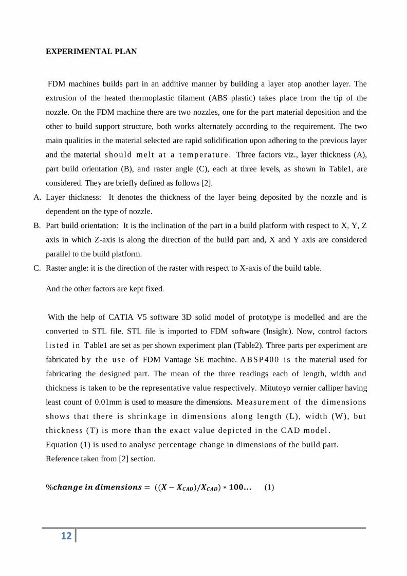
EXPERIMENTAL PLAN

FDM machines builds part in an additive manner by building a layer atop another layer. The

extrusion of the heated thermoplastic filament (ABS plastic) takes place from the tip of the

nozzle. On the FDM machine there are two nozzles, one for the part material deposition and the

other to build support structure, both works alternately according to the requirement. The two

main qualities in the material selected are rapid solidification upon adhering to the previous layer

and the material shou ld mel t a t a t empera tu re . Three factors viz., layer thickness (A),

part build orientation (B), and raster angle (C), each at three levels, as shown in Table1, are

considered. They are briefly defined as follows [2].

A. Layer thickness: It denotes the thickness of the layer being deposited by the nozzle and is

dependent on the type of nozzle.

B. Part build orientation: It is the inclination of the part in a build platform with respect to X, Y, Z

axis in which Z-axis is along the direction of the build part and, X and Y axis are considered

parallel to the build platform.

C. Raster angle: it is the direction of the raster with respect to X-axis of the build table.

And the other factors are kept fixed.

With the help of CATIA V5 software 3D solid model of prototype is modelled and are the

converted to STL file. STL file is imported to FDM software (Insight). Now, control factors

l i s t ed in Table1 are set as per shown experiment plan (Table2). Three parts per experiment are

fabricated by the use of FDM Vantage SE machine. ABSP400 i s t he material used for

fabricating the designed part. The mean of the three readings each of length, width and

thickness is taken to be the representative value respectively. Mitutoyo vernier calliper having

least count of 0.01mm is used to measure the dimensions. Measurement of the dimensions

shows that there is shrinkage in dimensions along length (L), width (W), but

thickness (T) is more than the exact value depicted in the CAD model .

Equation (1) is used to analyse percentage change in dimensions of the build part.

Reference taken from [2] section.

… (1)

13

1 .

FIGURE1: showing the Dimensions of test specimen in mm

EXPERIMENTAL DATA:

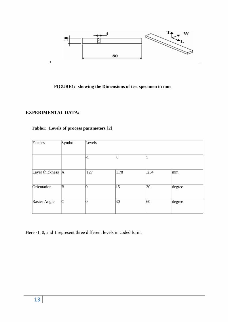
Table1: Levels of process parameters [2]

Factors Symbol Levels

-1 0 1

Layer thickness A .127 .178 .254 mm

Orientation B 0 15 30 degree

Raster Angle C 0 30 60 degree

Here -1, 0, and 1 represent three different levels in coded form.

14

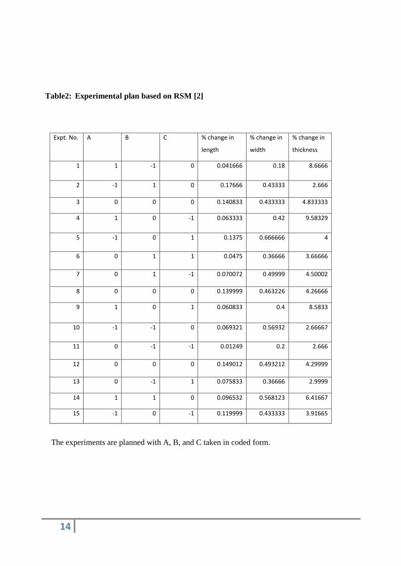
Table2: Experimental plan based on RSM [2]

Expt. No. A B C % change in

length

% change in

width

% change in

thickness

1 1 -1 0 0.041666 0.18 8.6666

2 -1 1 0 0.17666 0.43333 2.666

3 0 0 0 0.140833 0.433333 4.833333

4 1 0 -1 0.063333 0.42 9.58329

5 -1 0 1 0.1375 0.666666 4

6 0 1 1 0.0475 0.36666 3.66666

7 0 1 -1 0.070072 0.49999 4.50002

8 0 0 0 0.139999 0.463226 4.26666

9 1 0 1 0.060833 0.4 8.5833

10 -1 -1 0 0.069321 0.56932 2.66667

11 0 -1 -1 0.01249 0.2 2.666

12 0 0 0 0.149012 0.493212 4.29999

13 0 -1 1 0.075833 0.36666 2.9999

14 1 1 0 0.096532 0.568123 6.41667

15 -1 0 -1 0.119999 0.433333 3.91665

The experiments are planned with A, B, and C taken in coded form.

15

Chapter4

METHODOLOGY

16

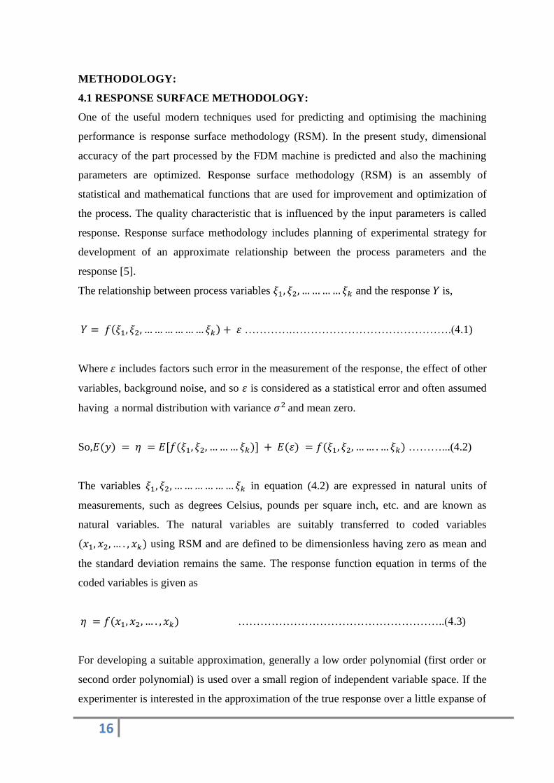
METHODOLOGY:

4.1 RESPONSE SURFACE METHODOLOGY:

One of the useful modern techniques used for predicting and optimising the machining

performance is response surface methodology (RSM). In the present study, dimensional

accuracy of the part processed by the FDM machine is predicted and also the machining

parameters are optimized. Response surface methodology (RSM) is an assembly of

statistical and mathematical functions that are used for improvement and optimization of

the process. The quality characteristic that is influenced by the input parameters is called

response. Response surface methodology includes planning of experimental strategy for

development of an approximate relationship between the process parameters and the

response [5].

The relationship between process variables and the response is,

………….…………………………………….(4.1)

Where includes factors such error in the measurement of the response, the effect of other

variables, background noise, and so is considered as a statistical error and often assumed

having a normal distribution with variance and mean zero.

So, ………...(4.2)

The variables in equation (4.2) are expressed in natural units of

measurements, such as degrees Celsius, pounds per square inch, etc. and are known as

natural variables. The natural variables are suitably transferred to coded variables

using RSM and are defined to be dimensionless having zero as mean and

the standard deviation remains the same. The response function equation in terms of the

coded variables is given as

………………………………………………..(4.3)

For developing a suitable approximation, generally a low order polynomial (first order or

second order polynomial) is used over a small region of independent variable space. If the

experimenter is interested in the approximation of the true response over a little expanse of

17

the independent variable space in the location where response function has little curvature,

than first order model is mostly used. The first-order model in terms of the coded variables

for the case having two independent variables, is shown below,

…….…………….. ……………………….(4.4)

If the interaction between the variables is considered then the first order model is easily

expressed as,

…….……… ………………………...(4.5)

Curvature is induced with the addition of the interaction between the variables. Due to

curvature, a second-order model is used because first order model is inadequate to

approximate the curvature of the true response surface which is generally strong. The

second-order model for the case of two variables is given by:

………(4.6)

This model would likely be useful as an approximation to the true response surface in a

relatively small region. The parameters can be easily estimated in the second order model

by using the method of least square.

In general, first order model can be written as

…………………………………….(4.7)

And the second order model can be given by,

∑

∑

∑ ∑

…………………………………(4.8)

Where ‟s are unknown parameters and for the estimation of the values of these parameters

experimental data is needed.

18

4.2 GENETIC ALGORITHM:

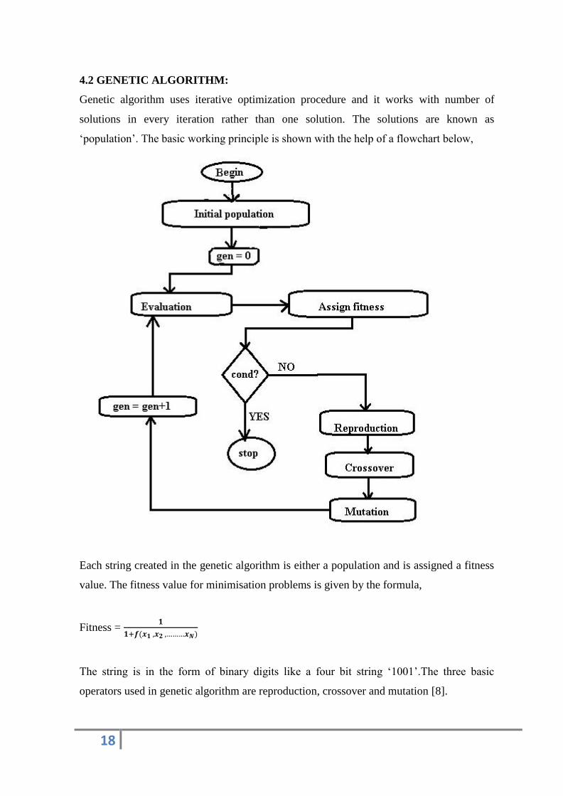
Genetic algorithm uses iterative optimization procedure and it works with number of

solutions in every iteration rather than one solution. The solutions are known as

„population‟. The basic working principle is shown with the help of a flowchart below,

Each string created in the genetic algorithm is either a population and is assigned a fitness

value. The fitness value for minimisation problems is given by the formula,

Fitness =

The string is in the form of binary digits like a four bit string „1001‟.The three basic

operators used in genetic algorithm are reproduction, crossover and mutation [8].

19

(A). Reproduction Reproduction selects good strings or ‟parents‟ from the initial

population with the best fitness value to reproduce offspring with best fitness. The parents

are selected by means of selection procedures where they go for reproduction [8]. There

are various methods available for selection of the parents such as proportionate selection

operator in which the string is selected having probability proportional to their

corresponding fitness, ranking selection scheme in which the strings are placed according

to the ascending order of their fitness value and the strings with the best fitness are

selected, tournament selection procedure in which two random strings are chosen from the

population and the one with the better fitness survives, etc.

The selected strings are placed in a mating pool from where reproduction phase starts

making the use of crossover operator.

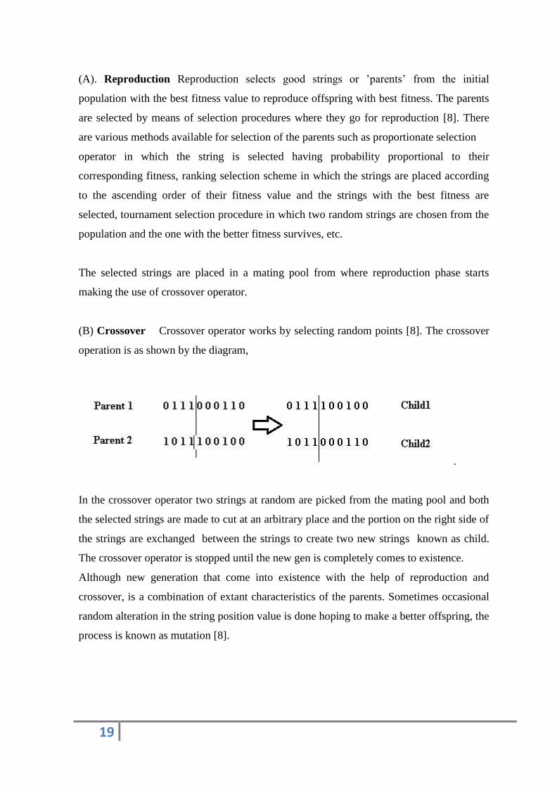
(B) Crossover Crossover operator works by selecting random points [8]. The crossover

operation is as shown by the diagram,

.

In the crossover operator two strings at random are picked from the mating pool and both

the selected strings are made to cut at an arbitrary place and the portion on the right side of

the strings are exchanged between the strings to create two new strings known as child.

The crossover operator is stopped until the new gen is completely comes to existence.

Although new generation that come into existence with the help of reproduction and

crossover, is a combination of extant characteristics of the parents. Sometimes occasional

random alteration in the string position value is done hoping to make a better offspring, the

process is known as mutation [8].

20

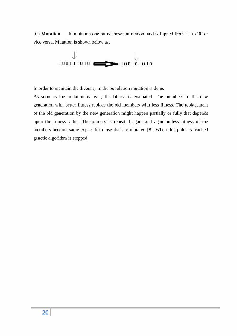
(C) Mutation In mutation one bit is chosen at random and is flipped from „1‟ to „0‟ or

vice versa. Mutation is shown below as,

In order to maintain the diversity in the population mutation is done.

As soon as the mutation is over, the fitness is evaluated. The members in the new

generation with better fitness replace the old members with less fitness. The replacement

of the old generation by the new generation might happen partially or fully that depends

upon the fitness value. The process is repeated again and again unless fitness of the

members become same expect for those that are mutated [8]. When this point is reached

genetic algorithm is stopped.

21

CHAPTER 5

RESULTS AND DISCUSSIONS

22

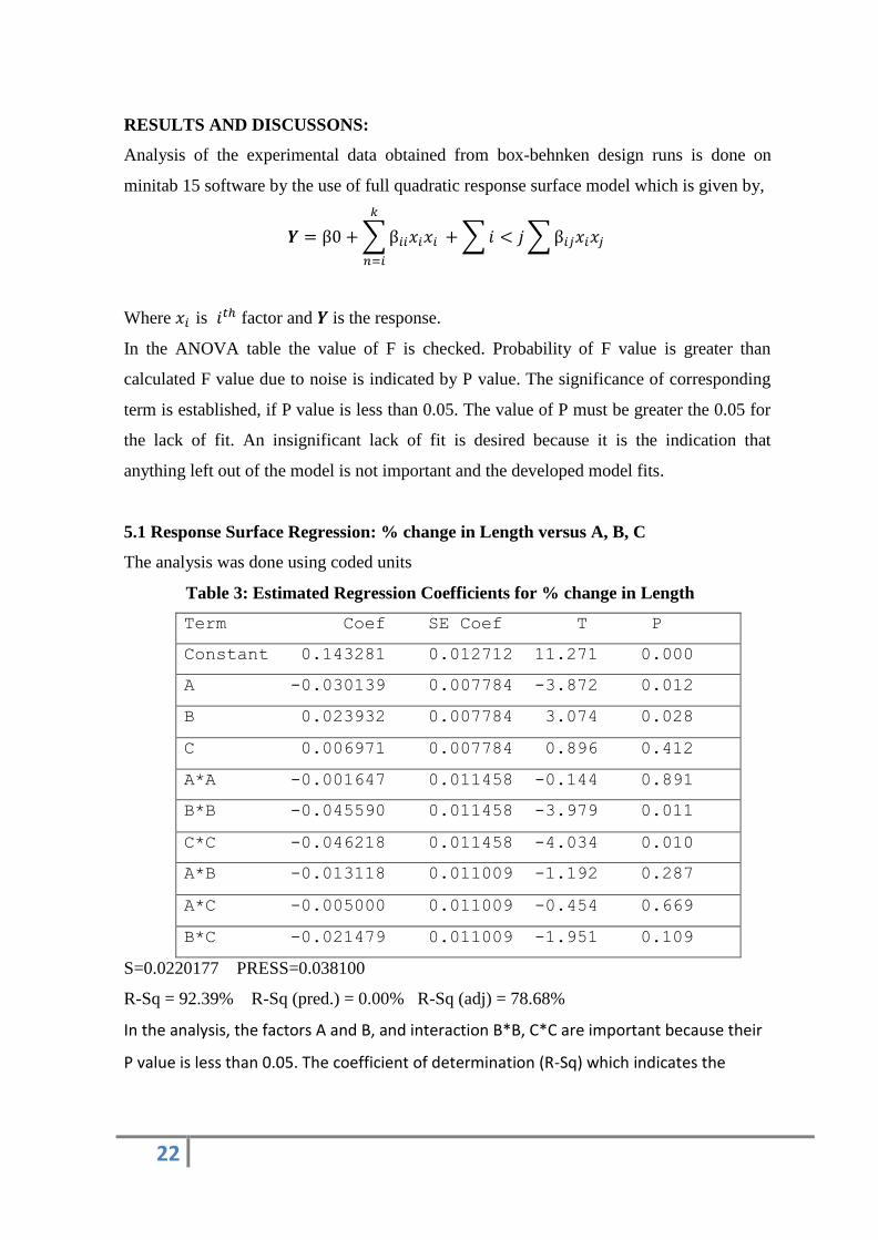
RESULTS AND DISCUSSONS:

Analysis of the experimental data obtained from box-behnken design runs is done on

minitab 15 software by the use of full quadratic response surface model which is given by,

∑

∑ ∑

Where is factor and is the response.

In the ANOVA table the value of F is checked. Probability of F value is greater than

calculated F value due to noise is indicated by P value. The significance of corresponding

term is established, if P value is less than 0.05. The value of P must be greater the 0.05 for

the lack of fit. An insignificant lack of fit is desired because it is the indication that

anything left out of the model is not important and the developed model fits.

5.1 Response Surface Regression: % change in Length versus A, B, C

The analysis was done using coded units

Table 3: Estimated Regression Coefficients for % change in Length

Term Coef SE Coef T P

Constant 0.143281 0.012712 11.271 0.000

A -0.030139 0.007784 -3.872 0.012

B 0.023932 0.007784 3.074 0.028

C 0.006971 0.007784 0.896 0.412

A*A -0.001647 0.011458 -0.144 0.891

B*B -0.045590 0.011458 -3.979 0.011

C*C -0.046218 0.011458 -4.034 0.010

A*B -0.013118 0.011009 -1.192 0.287

A*C -0.005000 0.011009 -0.454 0.669

B*C -0.021479 0.011009 -1.951 0.109

S=0.0220177 PRESS=0.038100

R-Sq = 92.39% R-Sq (pred.) = 0.00% R-Sq (adj) = 78.68%

In the analysis, the factors A and B, and interaction B*B, C*C are important because their

P value is less than 0.05. The coefficient of determination (R-Sq) which indicates the

23

goodness of fit for the model so the value of R-Sq = 92.39%, which indicate the high

significance of the model.

F(% change in Length) = 0.143281 - 0.030139*A + 0.023932*B – 0.045590*(B*B) –

0.0462181*(C*C)

Table4: Analysis of Variance for % change in Length:

Source DF Seq SS Adj SS Adj MS F P

Regression 9 0.029411 0.029411 0.003268 6.74 0.025

Linear 3 0.012238 0.012238 0.004079 8.41 0.021

Square 3 0.014540 0.014540 0.004847 10.00 0.015

Interaction 3 0.002634 0.002634 0.000878 1.81 0.262

Residual Error 5 0.002424 0.002424 0.000485

Lack-of-Fit 3 0.002374 0.002374 0.000791 31.91 0.031

Pure Error 2 0.000050 0.000050 0.000025

Total 14 0.031835

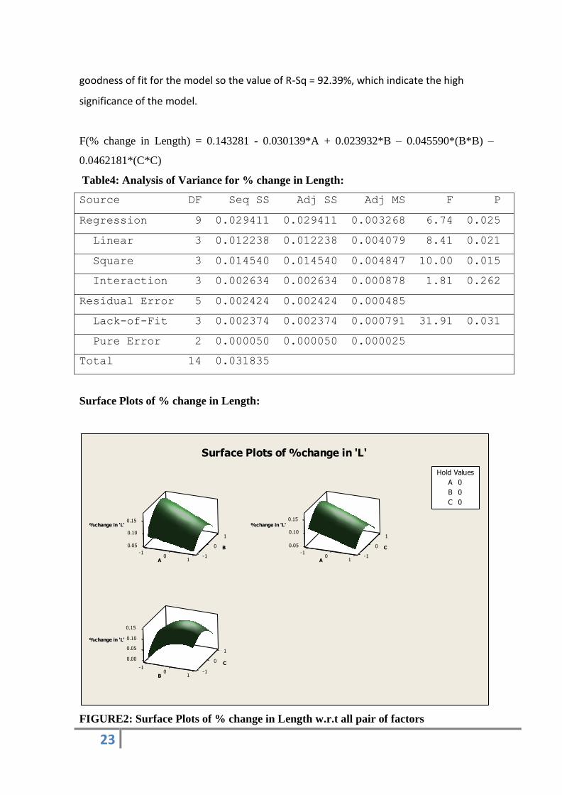
Surface Plots of % change in Length:

FIGURE2: Surface Plots of % change in Length w.r.t all pair of factors

1

0.05 0

0.10

0.15

-10 -1

1

%change in 'L'

B

A

1

0.05 0

0.10

0.15

-10 -1

1

%change in 'L'

C

A

1

0.00 0

0.05

0.10

-1

0.15

0 -11

%change in 'L'

C

B

A 0

B 0

C 0

Hold Values

Surface Plots of %change in 'L'

24

5.2 Response Surface Regression: % change in Width versus A, B, C

The analysis was done using coded units.

Table5: Estimated Regression Coefficients for % change in Width

Term Coef SE Coef T P

Constant 0.46326 0.02035 22.767 0.000

A -0.06682 0.01246 -5.362 0.003

B 0.06902 0.01246 5.539 0.003

C 0.03083 0.01246 2.475 0.056

A*A 0.04805 0.01834 2.620 0.047

B*B -0.07362 0.01834 -4.014 0.010

C*C -0.03131 0.01834 -1.707 0.148

A*B 0.13103 0.01762 7.436 0.001

A*C -0.06333 0.01762 -3.594 0.016

B*C -0.07500 0.01762 -4.256 0.008

S = 0.0352428 PRESS = 0.0747141

R-Sq = 97.29% R-Sq(pred) = 67.35% R-Sq(adj) = 92.40%

In the analysis, all the factors, and interaction A*A, B*B, A*B, A*C, B*C are important

because their P value is less than 0.05. The coefficient of determination (R-Sq) which

indicates the goodness of fit for the model so the value of R-Sq = 97.29%, which indicate

the high significance of the model.

F(% change in width) = 0.463257 - 0.0668157*A + 0.0690154*B + 0.0308329*C –

0.0480543*(A*A) – 0.0736180*(B*B) + 0.131028*(A*B) – 0.0633332*(A*C) –

0.0749975*(B*C)

25

Table 6: Analysis of Variance for % change in Width

Source DF Seq SS Adj SS Adj MS F P

Regression 9 0.222616 0.222616 0.024735 19.91 0.002

Linear 3 0.081425 0.081425 0.027142 21.85 0.003

Square 3 0.033974 0.033974 0.011325 9.12 0.018

Interaction 3 0.107217 0.107217 0.035739 28.77 0.001

Residual Error 5 0.006210 0.006210 0.001242

Lack-of-Fit 3 0.004418 0.004418 0.001473 1.64 0.400

Pure Error 2 0.001793 0.001793 0.000896

Total 14 0.228826

Surface Plots of %change in Width:

FIGURE3: Surface Plots of % change in Width w.r.t all pair of factors

10.2

0

0.4

-1

0.6

0 -11

%change in 'W

B

A

10.4

0

0.5

0.6

-10 -1

1

%change in 'W

C

A

1

0.20

0.3

0.4

-1

0.5

0 -11

%change in 'W

C

B

A 0

B 0

C 0

Hold Values

Surface Plots of %change in 'W'

26

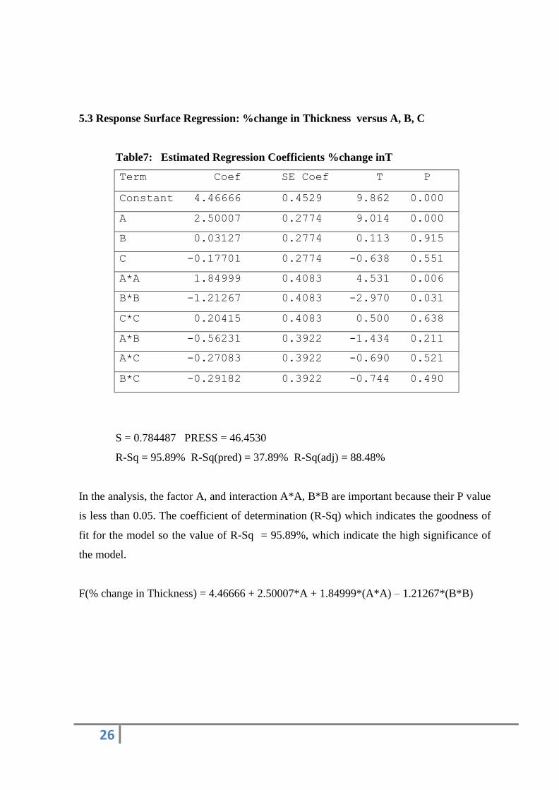
5.3 Response Surface Regression: %change in Thickness versus A, B, C

Table7: Estimated Regression Coefficients %change inT

Term Coef SE Coef T P

Constant 4.46666 0.4529 9.862 0.000

A 2.50007 0.2774 9.014 0.000

B 0.03127 0.2774 0.113 0.915

C -0.17701 0.2774 -0.638 0.551

A*A 1.84999 0.4083 4.531 0.006

B*B -1.21267 0.4083 -2.970 0.031

C*C 0.20415 0.4083 0.500 0.638

A*B -0.56231 0.3922 -1.434 0.211

A*C -0.27083 0.3922 -0.690 0.521

B*C -0.29182 0.3922 -0.744 0.490

S = 0.784487 PRESS = 46.4530

R-Sq = 95.89% R-Sq(pred) = 37.89% R-Sq(adj) = 88.48%

In the analysis, the factor A, and interaction A*A, B*B are important because their P value

is less than 0.05. The coefficient of determination (R-Sq) which indicates the goodness of

fit for the model so the value of R-Sq = 95.89%, which indicate the high significance of

the model.

F(% change in Thickness) = 4.46666 + 2.50007*A + 1.84999*(A*A) – 1.21267*(B*B)

27

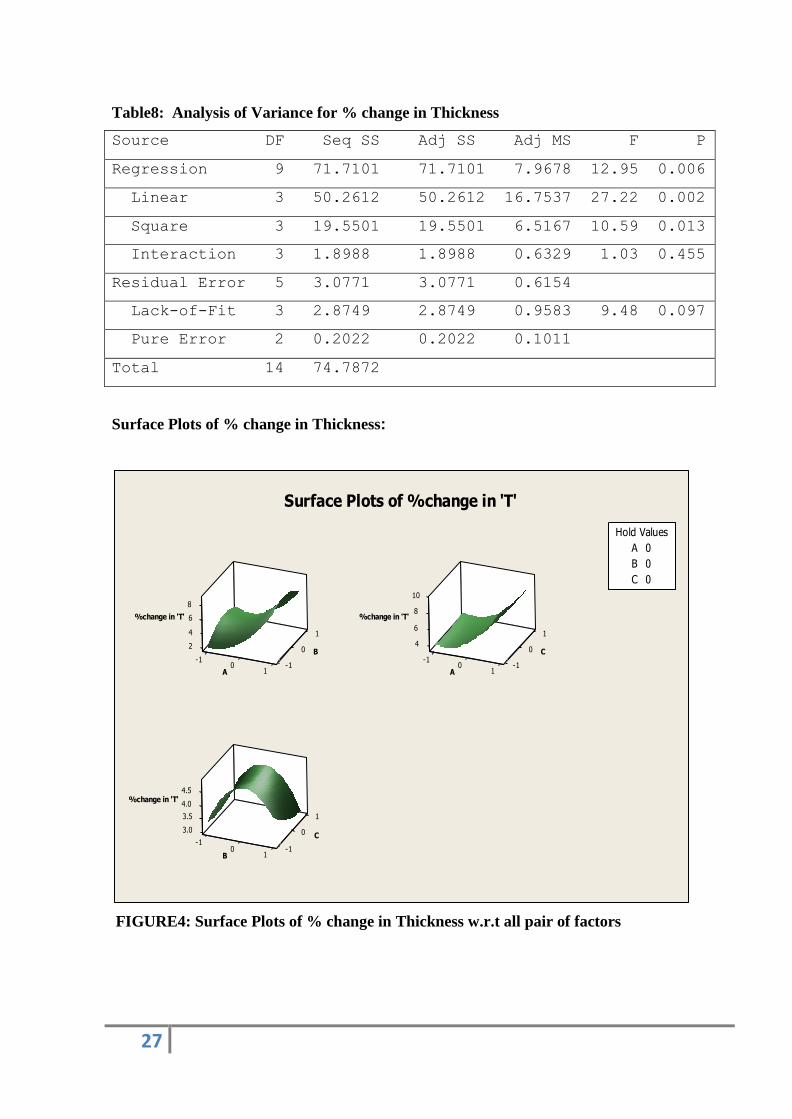
Table8: Analysis of Variance for % change in Thickness

Source DF Seq SS Adj SS Adj MS F P

Regression 9 71.7101 71.7101 7.9678 12.95 0.006

Linear 3 50.2612 50.2612 16.7537 27.22 0.002

Square 3 19.5501 19.5501 6.5167 10.59 0.013

Interaction 3 1.8988 1.8988 0.6329 1.03 0.455

Residual Error 5 3.0771 3.0771 0.6154

Lack-of-Fit 3 2.8749 2.8749 0.9583 9.48 0.097

Pure Error 2 0.2022 0.2022 0.1011

Total 14 74.7872

Surface Plots of % change in Thickness:

FIGURE4: Surface Plots of % change in Thickness w.r.t all pair of factors

1

2 0

4

6

-1

8

0 -11

%change in 'T'

B

A

1

40

6

8

-1

10

0 -11

%change in 'T'

C

A

1

3.0 0

3.5

4.0

4.5

-10 -1

1

%change in 'T'

C

B

A 0

B 0

C 0

Hold Values

Surface Plots of %change in 'T'

28

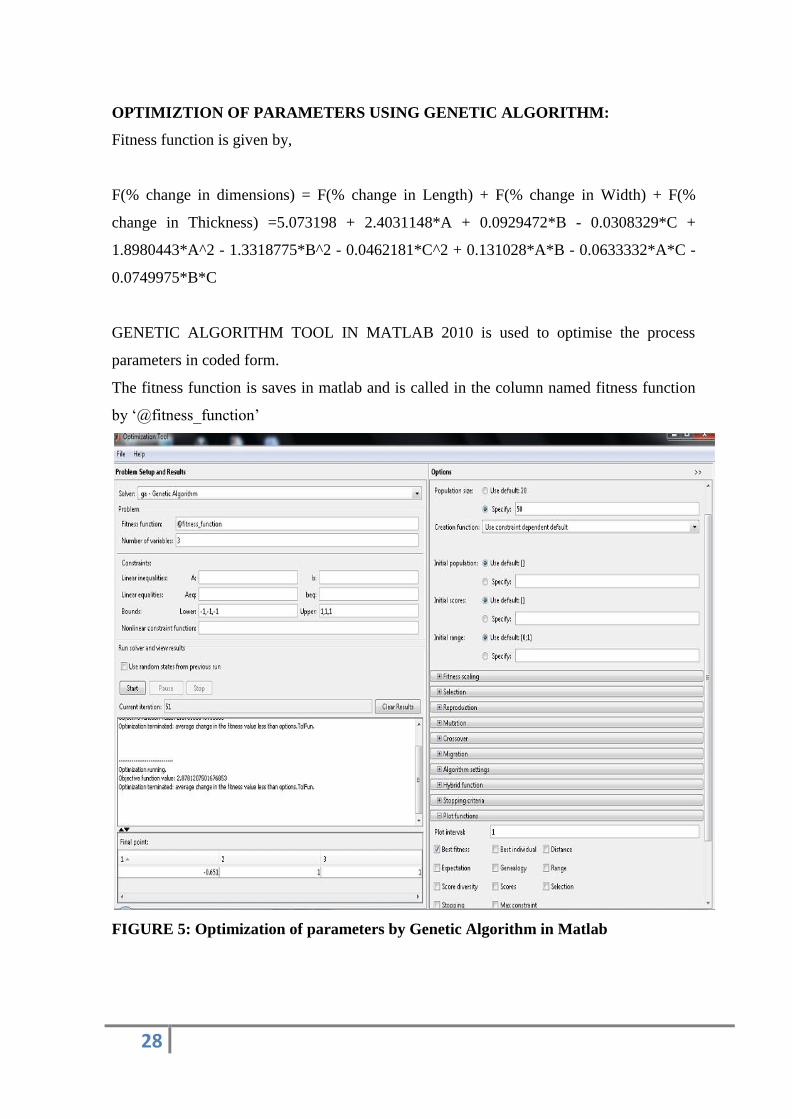
OPTIMIZTION OF PARAMETERS USING GENETIC ALGORITHM:

Fitness function is given by,

F(% change in dimensions) = F(% change in Length) + F(% change in Width) + F(%

change in Thickness) =5.073198 + 2.4031148*A + 0.0929472*B - 0.0308329*C +

1.8980443*A^2 - 1.3318775*B^2 - 0.0462181*C^2 + 0.131028*A*B - 0.0633332*A*C -

0.0749975*B*C

GENETIC ALGORITHM TOOL IN MATLAB 2010 is used to optimise the process

parameters in coded form.

The fitness function is saves in matlab and is called in the column named fitness function

by „@fitness_function‟

FIGURE 5: Optimization of parameters by Genetic Algorithm in Matlab

29

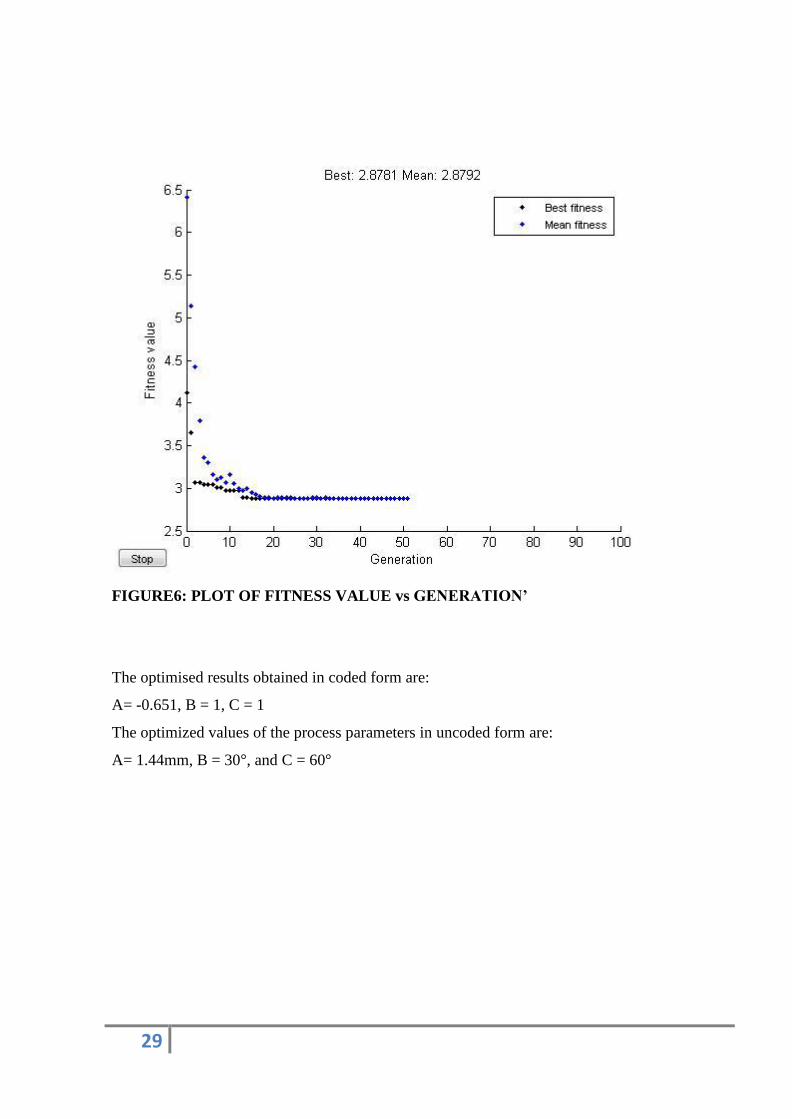
FIGURE6: PLOT OF FITNESS VALUE vs GENERATION’

The optimised results obtained in coded form are:

A= -0.651, B = 1, C = 1

The optimized values of the process parameters in uncoded form are:

A= 1.44mm, B = 30 , and C = 60

30

CONCLUSION:

In the present study, influence of three process parameters namely, layer thickness, part

build orientation, and raster angle each taken at three different levels are studied for the

accuracy of the dimensions of the FDM processed part. Response surface methodology‟s

design of experiment is used to make the experimental plan. It is observed that the

reduction dominates in length and width of the specimen but, the value of the thickness is

always more than the desired value. With the help of RSM significant factors and their

interaction are identified. In order to improve dimensional accuracy of the build part it is

required that the parts are manufactured in such a way that the minimum deviation of all

the dimensions from the actual value is obtained. Therefore optimum process variables

should be obtained through a structured method. The method of genetic algorithm is used

to get the optimum value of the process parameters so that dimensional accuracy is

increased. Genetic algorithm shows that layer thickness of , part build orientation

of and the raster angle of will fabricate the part with overall improvement in

accuracy of dimensions. Percentage deviation of is observed in dimensional

accuracy with the optimum values. Small percentage error establishes the fitness of the

present model.

31

References:

[1] Anitha R, Arunachalam S, Radhakrishnan P, (2001),”Critical parameters influencing the

quality of prototypes in fused deposition modelling”, Journal of Material Process

Technologies, Vol. 118, pp.(385-388).

[2] Sood,A.K., Ohdar,R.K. and Mahapatra,S.S., (2009), “Improving dimensional accuracy of

Fused Deposition Modelling processed part using grey Taguchi method”, Journal of

materials and design, Vol.30(9) , pp. (4243-4252).

[3] Pradhan,M.K and Biswas,C.K., (2009), “Modeling and Analysis of process parameters on

Surface Roughness in EDM of AISI D2 tool Steel by RSM Approach”, International

Journal of Engineering and Applied Sciences 5(1).

[4] Thrimurthulu k, Pandey,P.M. and Reddy,N.V., ”Optimum part deposition orientation in

fused deposition modelling”, International Journal of Machine Tools & Manufacture 44

(2004), pp.585–594.

[5] Carley,K.M., Kamneva,N.Y., and Reminga J (2004). Response surface methodology,

CASOS Technical report.

[6] Thrimurthulu k, Pandey,P.M. and Reddy,N.V., “Optimal part deposition orientation in

FDM by using a multicriteria genetic algorithm”, International journal of production

research, Vol. 42, No. 19, pp.4069-4089.

[7] Lee,B.H., Abdullah J and Khan,Z.A (2005), “Optimization of rapid prototyping

parameters for production of flexible ABS object, Journal of materials processing

technology, vol.169, pp.54–61

[8] Chattoraj N and Roy,J.S., (2007), “Application of Genetic Algorithm to the Optimization

of Gain of Magnetized Ferrite Microstrip Antenna”, Engineering Letters, 14:2,

EL_14_2_15 (Advance online publication: 16 May 2007)

32

[9] Zhou JackG, Daniel H, Chen Calvin C. (2000), “Parametric process optimization to

improve the accuracy of rapid prototyped stereolithography parts”, International Journal of

Machine Tools and Manufacture, Vol.40, pp.363–379.