Fused Deposition Modeling (FDM) Material Properties Characterization

ME 222 Final Project

John Michael Brock Michael Montero

Dan Odell Shad Roundy

Spring Semester May 5, 2000

1.0 Introduction Recent advances in the fields of Computer Aided Drafting (CAD) and Rapid Prototyping (RP)

have given designers the tools to rapidly generate an initial prototype from a concept. There are

currently several different RP technologies available, each with its own unique set of

competencies and limitations. In this paper, we seek to characterize some of the properties of

Stratasys� Fused Deposition Modeling (FDM) process, as well as the effects of varying some of

the build parameters.

Before we can discuss the properties of an FDM part, we must first discuss how the process

works. The first step in generating an FDM part is to create a three dimensional solid model.

This can be accomplished in many of the commonly available CAD packages. The part is then

exported to the FDM Quickslice software via the stereolithography (STL) format. This format

reduces the part to a set a triangles by tessellating it. The advantage of this is that it is a common

format that almost every CAD system can export, and reduces the part to its most basic

components. The disadvantage is that the part loses some resolution, as only triangles, and not

true arcs, splines, etc now represent it. However, these approximations are acceptable as long as

they are less than the inaccuracy inherent in the manufacturing process.

Once the STL file has been exported to Quickslice , it is then horizontally sliced into many thin

sections. These sections represent the two dimensional contours that the FDM process will

generate which, when stacked upon one another, will closely resemble the original part three

dimensional part. This sectioning approach is common to all currently available Rapid

Prototyping processes. Obviously, the thinner the sections, the more accurate the part. The

software then uses this information to generate the process plan that controls the FDM machine�s

hardware.

The Hardware for the FDM machine is represented in Figure 1.1. The concept is that a filament,

in our case ABS, is fed through a heating element, which heats it to a molten state. The filament

is then fed through a nozzle and deposited onto the part it is building. This aspect is not unlike

squeezing toothpaste from a tube. Since the material is extruded in a molten state, it fuses with

the material around it that has already been deposited. The head is then moved around in the X-

Y plane and deposits material according to the part requirements from the STL file. The head is

then moved vertically in the Z plane to begin depositing a new layer when the previous one is

completed. After a period of time, usually several hours, the head will have deposited a full

physical representation of the original CAD file.

It is interesting to note that this approach may require a support structure to be built beneath the

sections. If one horizontal slice overhangs the one below, it will simply fall to the substrate

when the FDM nozzle attempts to deposit it. The FDM machine possesses a second nozzle that

Figure 1.1 Fuse deposition modeling process.

extrudes support material for this purpose. The support material is similar to the model material,

but it is more brittle so that it may be easily removed after the model is completed. The FDM

machine builds support for any structure that has an overhang angle of less than 45° from

horizontal. If the angle is less than 45°, more than one half of one bead is overhanging the slice

below it, and therefore is likely to fall.

This process results in a part with unique characteristics. While it is much tougher than parts

made by other RP processes (such as SLA), we have still experienced brittle fractures at

relatively low loads. This experience goes against the blanket claim that Stratasys makes that

FDM parts possess 70% of the strength of solid ABS parts. Also, this claim is very vague as the

yield strength of ABS can vary from 29 MPa to 124 MPa. In addition, it is very clear that the

FDM process deposits material in a direction way; which results in non-isotropic parts. With

these problems in mind, we set out to characterize the material behavior of FDM parts, as well as

the effects of some of the process control parameters.

2.0 Build Parameter Considerations To begin our experiment, we first identified the process control parameters that were likely to

affect the properties of FDM parts. The parameters we selected are listed below:

Bead (or road) width: This is the thickness of the bead (or road) that the FDM nozzle

deposits. It can vary from .012� to .0396� for the T12 nozzle which is currently installed

on our Stratasys FDM 1650 machine.

Air Gap: This is the space between the beads of FDM material. The default is zero,

meaning that the beads just touch. It can be modified to leave a positive gap, which

means that the beads of material do not touch. This results in a loosely packed structure

that builds rapidly. It can also be modified to leave a negative gap, meaning that two

beads partially occupy the same space. This results in a dense structure which requires a

longer build time.

Model Build Temperature: The temperature of the heating element for the model

material. This controls how molten the material is as it is extruded from the nozzle.

Raster Orientation: The direction of the beads of material (roads) relative to the

loading of the part.

Color: FDM ABS material is available in a variety of colors: white, blue, black, yellow,

green, and red.

We decided to neglect the possible affects of envelope temperature (the temperature of the air

around the part), slice height (which is similar to bead width in the vertical direction), and nozzle

diameter (the width of the hole through which the material extrudes). These parameters seemed

either duplicates of parameters we selected, or did not seem to have a relevant connection to the

final material properties.

3.0 Experiment Setup To begin testing, we built a series of samples on the FDM machine (see Design of Experiment

section for more detail). Examples of test parts can be seen in Figures 3.1 (Quickslice views of

parts) and 3.2 (actual test specimens with loading directions indicated). Note that the loading

directions in Figure 3.2 define the terminology that will be used throughout the remainder of this

paper.

Figure 3.1 Quickslice SML file showing samples with bead-width, air gap, and raster orientation variation.

Figure 3.2 Actual tensile specimens in axial (1) and transverse (2) load directions

Transverse

Axial

To test the properties of our test samples, we used an Instron load frame to load the samples in

tension. We then collected the load and extension data of the sample as it was loaded. To

measure the strain of our sample, we used an extensometer (see Figure 3.3). This device limited

our max test strain to twenty percent. As the extensometer only measures strain between its

blades, we also collected displacement data at the grips for comparison.

When we began our testing, we used samples that conformed to the ASTM D-638 97, type I

standard (a dog-bone shaped sample). However, we quickly ran into problems with this

approach. As you can see in Figures 3.4 and 3.5, the dog-bone shape added complications to the

loading of the parts that caused them to fail pre-maturely. We attempted to use two different

approaches with this shape: a raster approach, and a contour approach. The raster approach

yielded a series of infinitely small stress concentrations at the site of what was supposed to be a

large, stress concentration reducing, three-inch radius. The contour approach yielded stress-

concentrating gaps in the middle of the part, as well as a non-axial stress state at the radii. While

the contours were better than the rasters, we decided to abandon the dog-bone shape in favor of a

simple rectangle that possessed no potential stress concentrators at all. We landed on a sample

Figure 3.3 Instron load frame set-up.

Instron Grips

Extensometer

Test Sample

size of Width .375� x Length 4.00� x Thickness .125� for axial samples, and a thickness of .25�

with the same width and length for our transverse samples.

Figure 3.4 Trouble with stress concentration - 3” radius actually infinitely small.

Figure 3.5 Trouble with contours - Gaps, stress concentration, and (2) loading.

4.0 Design of Experiment (DOE) The goal of the experiment is to see how changing multiple design and process variables effects

tensile strength within FDM tensile specimens. As mentioned before, the actual variables

selected for the experiment are chosen from a larger set based on intuitive knowledge of each

parameter. Figure 4.1 shows the larger set of variables and under what domain or classification

they fall under.

The five variables selected are actually from three different classifications: unprocessed ABS,

FDM build specifications, and FDM environment. The five variables are air gap, bead width,

model temperature, ABS color, and raster orientation. Amongst the five variables, one variable

is qualitative (ABS color) whereas the remaining four are quantitative parameters. The next step

in the setup of the DOE is to determine the type of resolution for the experiment and the number

of levels for each variable.

Unprocessed ABS

FDM Build Specifications

Specimen Positioning

FDM Environment/Machine

RasterBead Width

Air Gap

Contouring

Model Temperature

Envelope Temperature

Density

X-Y Position w/in Envelope

Color

Nozzle Diameter

Material

Figure 4.1 Fishbone diagram of potential factors influencing tensile strength

!!!!

!!!!

!!!!!!!!

!!!!

The experiment should yield unambiguous results between the estimation of variable effects as

well as be conducted within a reasonable amount of time. Build time for each tensile specimen

is taken into consideration as well as the time needed to perform the fracture test. Therefore,

minimizing the number of tests within the experiment while providing clear estimations of the

effects are the highest of priority. Keeping that in mind, a fractional factorial DOE is selected to

meet both requirements.

We hope to see a linear behavior of the response (tensile strength) as a function of the 5

variables. For that reason, each parameter will have two levels set at a high (+1) and a low (-1).

In order to set the appropriate levels for each variable, preliminary tests were conducted for each

variable to define its range. Each variable was varied independently from all the others and the

tensile strength was measured. The results of these preliminary tests gave us a suitable range for

the two levels of each parameter. Figure 4.2 shows the parameters, their associated symbols, and

their level settings.

By only having two levels, a 25-1 design will provide a high-resolution (V) and only 16 required

test conditions. The resolution of the design is an indicator of the degree of confounding within

the effect estimations for each variable. Confounding is the inability to distinguish one variable

effect from another. With a resolution V design, we will have 16 estimates of effects whereby

the main effects are confounded with 4-factor interactions and 2-factor interactions are

confounded with 3-factor interactions. The resolution number represents the smallest word

within the defining relation of a design. The defining relation is used to determine which effects

are confounded with each other. In order to obtain a defining relation, a generator is needed and

can be selected from the possible combinations of variables. In our design, variable E (or raster

Variable Symbol Low(-) High(+)Air Gap (in.) A 0.0000 -0.0020

Road Width (in.) B 0.02 0.0396Model Temperature (C) C 270 280

ABS Color D Blue WhiteOrientation of Rasters E Transverse Axial

Levels

Figure 4.2 Variable symbols and level settings.

orientation) will be our generator. We choose E = ABCD and from our generator we can obtain

our defining relation by simply multiplying each side by E. Therefore, the defining relation is the

following: I = ABCDE. We can now multiply all main effects and multi-factor interaction

effects by the defining relation to reveal the confounding terms within each effect estimate.

Figure 4.3 shows the following process of obtaining a resolution V DOE.

Not only does the generator and defining relation help deriving the effect estimates, but they also

help in setting the appropriate test conditions for the design matrix. Since our generator is E =

ABCD, then the test conditions for parameter E will be defined by the product of coded units (+1

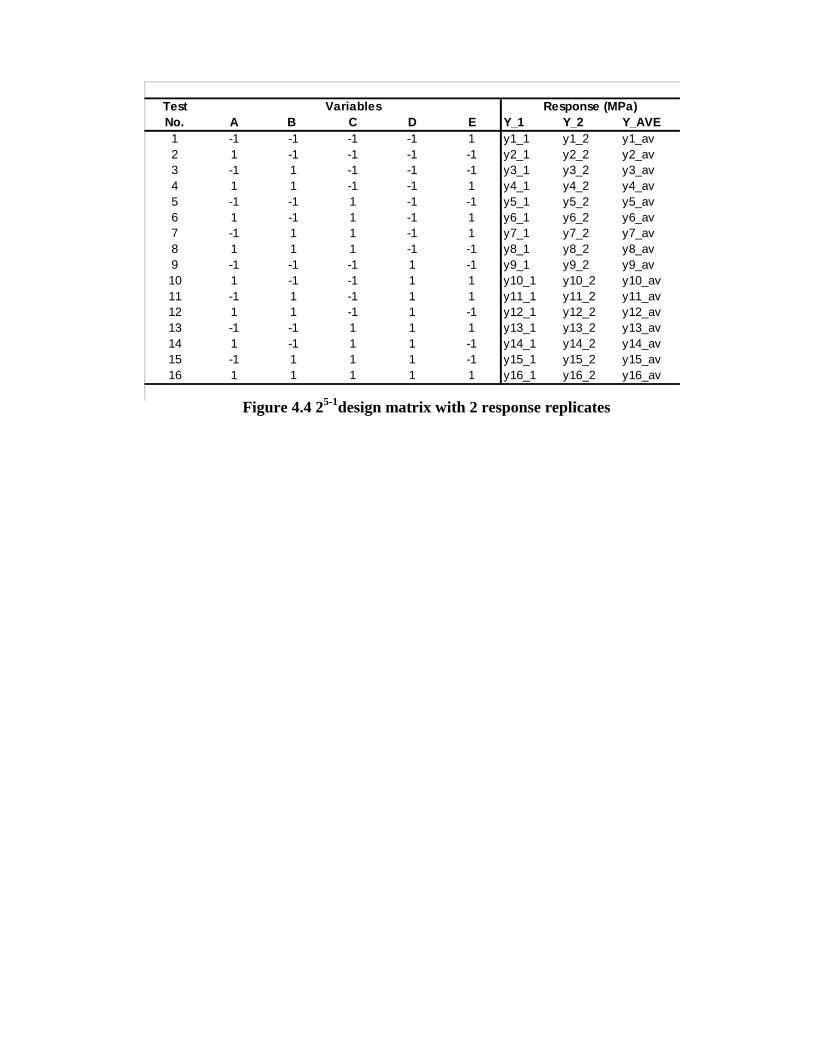
and �1) of columns A, B, C, and D. Figure 4.4 shows the design matrix. With only 16 test

conditions, it was decided to replicate each one in order to calculate an estimate of the standard

error within our experiment. The variance calculated will be used in conjunction with the

student-t distribution to produce confidence intervals (α = 97.5%) of each effect estimate to

verify statistical significance. The final design contains a total of 32 test specimens, which is an

advantage over a full factorial design (25) which contains the same number of runs but lacks the

estimate of error. The following section shows the results of the DOE but does not go deep into

the computation of the effects. Further details can be found in Box and Hunter�s Statistics for

Experimenters.

Factors: A, B, C, D, E Generator: E = ABCD Defining relation: E*E = ABCD*E I = ABCDE E1 = EA + EA*I = EA + EA*ABCDE = EA + EBCDE . .

. . E12 = EAB + EAB*I = EAB + EAB*ABCDE = EAB + ECDE

Main & 4-factor interaction confounding

2-factor interaction & 4-factor interaction confounding

Effect estimates for each variable

Figure 4.3 Defining effect estimates using defining relation for resolution V DOE.

Smallest word = 5, so resolution is V

TestNo. A B C D E Y_1 Y_2 Y_AVE1 -1 -1 -1 -1 1 y1_1 y1_2 y1_av2 1 -1 -1 -1 -1 y2_1 y2_2 y2_av3 -1 1 -1 -1 -1 y3_1 y3_2 y3_av4 1 1 -1 -1 1 y4_1 y4_2 y4_av5 -1 -1 1 -1 -1 y5_1 y5_2 y5_av6 1 -1 1 -1 1 y6_1 y6_2 y6_av7 -1 1 1 -1 1 y7_1 y7_2 y7_av8 1 1 1 -1 -1 y8_1 y8_2 y8_av9 -1 -1 -1 1 -1 y9_1 y9_2 y9_av10 1 -1 -1 1 1 y10_1 y10_2 y10_av11 -1 1 -1 1 1 y11_1 y11_2 y11_av12 1 1 -1 1 -1 y12_1 y12_2 y12_av13 -1 -1 1 1 1 y13_1 y13_2 y13_av14 1 -1 1 1 -1 y14_1 y14_2 y14_av15 -1 1 1 1 -1 y15_1 y15_2 y15_av16 1 1 1 1 1 y16_1 y16_2 y16_av

Response (MPa)Variables

Figure 4.4 25-1design matrix with 2 response replicates

5.0 Analysis of DOE Figure 5.1 shows the tensile strengths for each test condition with 2 replicates. The average

response was used in calculating all 16 effects. The variance among the responses within each

test was calculated. Tests 2, 3, 5, 9, and 12 show large variations and can be contributed to the

random defects which exist between layers of the tensile specimen. These random defects make

the bulk specimen susceptible to stress concentrations especially when raster orientation (E) is

traverse (-1). These large variations may inflate the overall effect variance.

Figure 5.2 shows the estimates of effects. Since 3-factor interactions or higher have a low

probability of occurring (or showing large effects) due to the nature of the FDM machine, we

assume that they are negligible. This assumption may not hold true and is highly dependent on

the mechanism under questions. For instance, DOE�s that investigate chemical compositions

will include higher order interactions since the nature of the mechanism presents a higher

probability of yielding significant higher order interactions. Keeping that in mind, Figure 5.2

shows how each effect can be resolved or essentially three-factor or higher interactions can be

removed from the estimate.

Test A B C D E Y1(MPa) Y2(MPa) YAVE R si

2 DOF 1 -1 -1 -1 -1 1 19.17 20.02 19.60 -0.85 0.36 1 2 1 -1 -1 -1 -1 10.00 14.08 12.04 -4.08 8.32 1 3 -1 1 -1 -1 -1 1.14 2.96 2.05 -1.82 1.65 1 4 1 1 -1 -1 1 22.77 23.20 22.98 -0.42 0.09 1 5 -1 -1 1 -1 -1 3.40 1.54 2.47 1.86 1.73 1 6 1 -1 1 -1 1 21.57 21.42 21.50 0.15 0.01 1 7 -1 1 1 -1 1 20.93 20.48 20.71 0.45 0.10 1 8 1 1 1 -1 -1 11.38 10.98 11.18 0.40 0.08 1 9 -1 -1 -1 1 -1 1.42 3.17 2.30 -1.75 1.53 1

10 1 -1 -1 1 1 22.99 22.50 22.74 0.50 0.12 1 11 -1 1 -1 1 1 20.77 21.39 21.08 -0.63 0.20 1 12 1 1 -1 1 -1 5.42 8.18 6.80 -2.77 3.83 1 13 -1 -1 1 1 1 20.27 19.90 20.08 0.37 0.07 1 14 1 -1 1 1 -1 12.07 12.92 12.50 -0.85 0.36 1 15 -1 1 1 1 -1 0.90 1.98 1.44 -1.08 0.59 1 16 1 1 1 1 1 23.50 23.30 23.40 0.20 0.02 1

Figure 5.1 DOE responses, average responses, ranges, test variances, and degrees of freedom

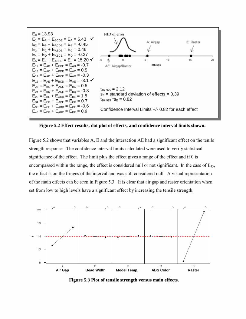
Figure 5.2 shows that variables A, E and the interaction AE had a significant effect on the tenile

strength response. The confidence interval limits calculated were used to verify statistical

significance of the effect. The limit plus the effect gives a range of the effect and if 0 is

encompassed within the range, the effect is considered null or not significant. In the case of E45,

the effect is on the fringes of the interval and was still considered null. A visual representation

of the main effects can be seen in Figure 5.3. It is clear that air gap and raster orientation when

set from low to high levels have a significant effect by increasing the tensile strength.

E0 = 13.93 E1 = EA + EBCDE = EA = 5.43 !!!! E2 = EB + EACDE = EB = -0.45 E3 = EC + EABDE = EC = 0.46 E4 = ED + EABCE = ED = -0.27 E5 = EE + EABCD = EE = 15.20 !!!! E12 = EAB + ECDE = EAB = -0.7 E13 = EAC + EBDE = EAC = 0.5 E14 = EAD + EBCE = EAD = -0.3 E15 = EAE + EBCD = EAE = -3.1 !!!! E23 = EBC + EADE = EBC = 0.5 E24 = EBD + EACE = EBD = -0.8 E25 = EBE + EACD = EBE = 1.5 E34 = ECD + EABE = ECD = 0.7 E35 = ECE + EABD = ECE = -0.6 E45 = EDE + EABC = EDE = 0.9

t16,.975 = 2.12 sE = standard deviation of effects = 0.39 t16,.975 *sE = 0.82 Confidence Interval Limits +/- 0.82 for each effect

Figure 5.2 Effect results, dot plot of effects, and confidence interval limits shown.

NID of error

Figure 5.3 Plot of tensile strength versus main effects.

Air Gap Raster Bead Width Model Temp. ABS Color

If we look at the effect of AE on tensile strength in Figure 5.4, a strong interaction between both

variables exists. When the tensile specimen has the roads oriented in the traverse direction (-1)

the air gap will influence the tensile strength greatly. On the other hand, when the roads are

oriented axially (+1), the air gap effect is less.

6.0 Predictive Model from DOE The DOE not only determines which effects are significant, but it also formulates a mathematical

model using the effects as coefficients for the significant variables. The following formula (1)

shows tensile strength as a function of air gap and raster orientation.

y = tensile strength = 13.9 + 2.7A + 7.6E - 1.6A*E (1)

The model can be used to interpolate values or extrapolate. Further experiments utilize the model

to eventually construct a surface response in order to find an optimum. We decided to use the

model as a method of predicting tensile strengths by conducting four additional tests. The test

levels and results are shown in Table 6.1. The model holds up well when raster orientation is

held axially and air gap is varied in Test 1 and 2. The error for Test 1 and 2 are 6.3 % and 4.4%

Traverse Axial

Negative Air Gap

Zero Air Gap

Raster

Figure 5.4 Interaction plot of tensile strength versus air gap/raster interaction.

respectively. On the other hand, the model does not hold up well for Test 3 showing a large

error between the tensile strengths. During actual fracture test, the tensile specimen for Test 3

appeared to have a defect present within the layers of the material. During the tensile test, the

specimen fractured in the region of the defect very quickly with very little strain. The large error

in Test 3 could be attributed to this initial defect present. Test 4 yields reasonably close tensile

strengths between the predictive and experimental values with an error of 6.2 %.

Test No. A: Air Gap (in.) E: Raster

(orient.) Predictive Tensile Strength (MPa)

Experimental Tensile Strength (MPa)

1 0.000 Axial 20.4 19.2 2 -0.001 Axial 21.5 20.6 3 0.000 45° 11.2 3.3 4 -0.001 45° 16.6 17.7

Table 6.1 Predictive model versus experimental results

7.0 Further Analysis In practice, most FDM parts are made with a crisscross raster in which the orientation of the

beads alternates from +45º to -45º from layer to layer. Some crisscross raster specimens were

built and tested in addition to the main factorial experiment. The two purposes for these tests

were first to test whether the results for the main factorial experiment hold for a crisscross raster,

and second to verify the predictive

model, which will be explained in detail

later. An example stress vs. strain curve

for these tests is shown in Figure (7.1).

Notice that there is a significant amount

of plastic behavior for these parts. The

factorial experiment indicated that the

only two significant factors are raster

orientation and air gap. Since the raster

orientation is already set for a crisscross

raster, the only factor varied for these

tests was air gap. As shown in Figure

(5.1), the parts with a negative air gap are significantly stronger. Also, the tensile strength

predicted by the model from the factorial experiment matches the actual data reasonably well.

The elastic modulus was measured for the parts that were tested as part of the factorial

experiment and for the crisscross raster parts. These results are summarized in Table (7.1). The

parts built with an axial raster orientation were significantly more stiff than those built with

transverse raster orientation. Also, the crisscross raster parts with a negative air gap were more

stiff than those built with zero air gap. Interestingly, air gap did not have a significant effect on

the elastic modulus for the axial or transverse parts. Bulk ABS has an elastic modulus of about 2

GPa, or about twice that of the FDM parts built out of ABS. Figure (7.2) shows a stress vs.

strain curve for part built with axial rasters. Notice the sharp peak at the end of the elastic region

Y(measured) Y(predicted)Zero Air Gap 11.7 MPa 11.2 MPa

-.002 in. Air Gap 18.2 Mpa 16.6 MPa

Stress vs. Strain (raster - 0 air gap)

0

2

4

6

8

10

12

14

0 1 2 3 4 5 6% Strain

Stre

ss (M

Pa)

Figure (7.1)

Axial Transverse Crisscross 0 Air Gap Crisscross -.002 Air GapE (GPa) 1.6 1.0 1.48 0.8

Table (7.1)

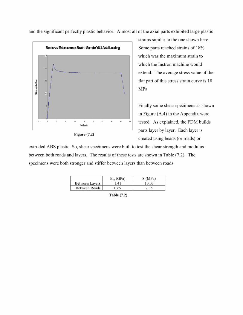
and the significant perfectly plastic behavior. Almost all of the axial parts exhibited large plastic

strains similar to the one shown here.

Some parts reached strains of 18%,

which was the maximum strain to

which the Instron machine would

extend. The average stress value of the

flat part of this stress strain curve is 18

MPa.

Finally some shear specimens as shown

in Figure (A.4) in the Appendix were

tested. As explained, the FDM builds

parts layer by layer. Each layer is

created using beads (or roads) or

extruded ABS plastic. So, shear specimens were built to test the shear strength and modulus

between both roads and layers. The results of these tests are shown in Table (7.2). The

specimens were both stronger and stiffer between layers than between roads.

Stress vs. Extensometer Strain - Sample Y6-1 Axial Loading

0

5

10

15

20

25

-2 0 2 4 6 8 10 12 14 16 18

% Strain

Stre

ss(M

Pa)

Figure (7.2)

Esh (GPa) S (MPa)Between Layers 1.41 10.03Between Roads 0.69 7.35

Table (7.2)

8.0 Classical Plate Theory Classical plate theory applies to bodies for which one dimension is significantly smaller than the

other two. Several assumptions about the deformation of such a body are made. The

displacement in the z-direction, w, of a point is assumed to be independent of its z-position.

Further, the displacement of a point in the x-direction, u, (or y-direction, v) is assumed to be the

sum of the midplane displacement and the distance from the midplane multiplied by the slope of

the midplane. In other words, plane sections remain plane and normals remain normal.

A critical aspect of classical plate theory is seen when strain-displacement relations are applied

to the above displacement assumptions. The result is that all components of strain in the z-

direction, the normal and transverse shear strains, are zero. That means that all loads are carried

by in plane stresses, including loads applied in the z-direction. Integrating the in plane stresses

over the thickness of the plate, z, gives the applied loads in the x- and y-directions. If the in

plane normal and shear stresses are multiplied by their z position and then integrated the applied

moments are found. With these relations, measured quantities, forces and displacements, can be

related to stresses and strains, which in practice are hard to measure.

8.1 Laminated Plate Theory Laminated plate theory extends classical plate theory for bodies that are comprised of layers,

called plies, which may or may not have similar properties. The theory is generally applied to

materials that are either orthotropic or transversely isotropic. Consequently the material

properties of the body may not be uniform throughout the thickness, instead just throughout each

layer. Laminated plate theory only considers the material properties of a plate as a whole. For a

composite, where the layers are comprised of fibers and matrix, the bulk behavior of the

composite is only of interest. For orthotropic and transversely isotropic materials the properties

are a function of orientation of the ply. A ply coordinate system is defined with the 1-direction

aligned with the direction of maximum stiffness, and the 2-direction rotated 90 degrees in plane.

To determine the properties in body coordinates of an arbitrarily oriented ply, a fourth order

tensor rotation of the plane strain reduced stiffness matrix is performed.

Figure 8.1 Book-keeping scheme of ply properties and positions. [1]

Just as was discussed in classical plate theory, the external moments and forces that cause

stresses in the plate are found by integrating the stresses over the stresses multiplied by their

vertical position over the thickness, respectively. An assumption is made that there is perfect

bonding between all layers of the composite, and as a result the strain is continuous throughout

the thickness. Because the material properties are only piecewise constant throughout the

thickness, the stresses can be discontinuous at the interfaces between layers. Therefore the

integration must be broken up and performed layer by layer. The stress is found by multiplying

the reduced stiffness matrix in body coordinates of each ply by the midplane strain of each ply.

As previously mentioned the midply strain is the sum of the midplane strain and the effect of

rotation of the midplane. The sum of the integrals is equal to the externally applied loads.

However, the external loads that will be applied to a body are usually known while the

displacements and hence stress and strain are unknown. If the above analysis is inverted, the

midplane strains and curvatures are equal to the inverted plane strain reduced stiffness matrices

multiplied by the force matrix. From the midplane strains and curvatures the midply strains in

body coordinates can be deduced. Multiplying by the plane strain reduced stiffness gives the

midply stress for each ply. Using second order tensor rotations, the stresses and strains in the ply

coordinates are determined.

8.2 Tsai Wu Failure Criterion Tsai Wu Failure Criterion is used to predict yield in orthotropic materials. It is a relation that

was developed from empirical data based upon failure of hundreds of materials. The hypothesis

is that a material fails when the ratio of applied stress to yield strength is equal to one. Tsai Wu

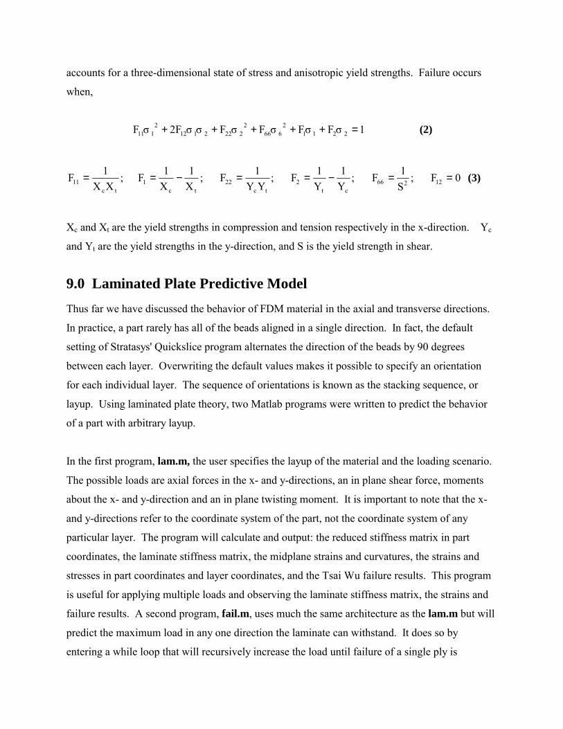
accounts for a three-dimensional state of stress and anisotropic yield strengths. Failure occurs

when,

1σFσFσFσFσσ2FσF 22112

6662

22221122

111 =+++++ (2)

;XX

1Ftc

11 = ;X1

X1F

tc1 −= ;

YY1F

tc22 = ;

Y1

Y1F

ct2 −= ;

S1F 266 = 0F12 = (3)

Xc and Xt are the yield strengths in compression and tension respectively in the x-direction. Yc

and Yt are the yield strengths in the y-direction, and S is the yield strength in shear.

9.0 Laminated Plate Predictive Model Thus far we have discussed the behavior of FDM material in the axial and transverse directions.

In practice, a part rarely has all of the beads aligned in a single direction. In fact, the default

setting of Stratasys' Quickslice program alternates the direction of the beads by 90 degrees

between each layer. Overwriting the default values makes it possible to specify an orientation

for each individual layer. The sequence of orientations is known as the stacking sequence, or

layup. Using laminated plate theory, two Matlab programs were written to predict the behavior

of a part with arbitrary layup.

In the first program, lam.m, the user specifies the layup of the material and the loading scenario.

The possible loads are axial forces in the x- and y-directions, an in plane shear force, moments

about the x- and y-direction and an in plane twisting moment. It is important to note that the x-

and y-directions refer to the coordinate system of the part, not the coordinate system of any

particular layer. The program will calculate and output: the reduced stiffness matrix in part

coordinates, the laminate stiffness matrix, the midplane strains and curvatures, the strains and

stresses in part coordinates and layer coordinates, and the Tsai Wu failure results. This program

is useful for applying multiple loads and observing the laminate stiffness matrix, the strains and

failure results. A second program, fail.m, uses much the same architecture as the lam.m but will

predict the maximum load in any one direction the laminate can withstand. It does so by

entering a while loop that will recursively increase the load until failure of a single ply is

observed with a resolution of one hundredth of a MPa. This program is useful for determining

the load at which a part will fail if the layup and loading direction are known but the magnitude

of the loading is unknown.

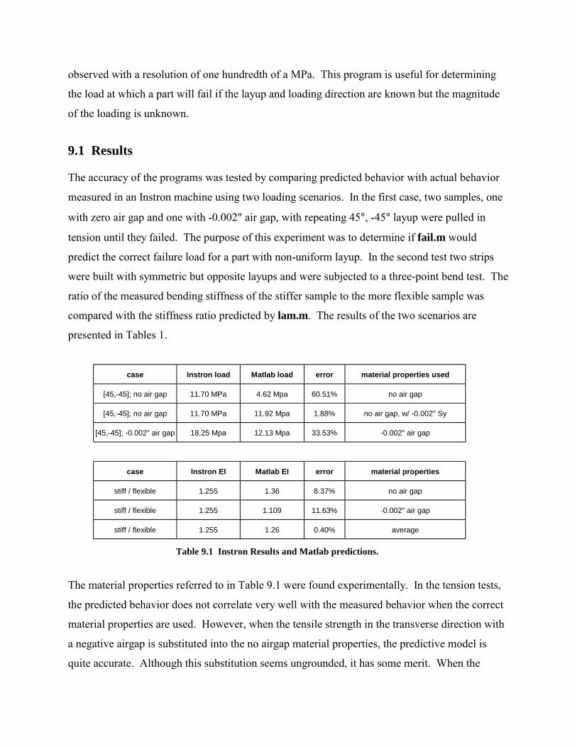
9.1 Results The accuracy of the programs was tested by comparing predicted behavior with actual behavior

measured in an Instron machine using two loading scenarios. In the first case, two samples, one

with zero air gap and one with -0.002" air gap, with repeating 45°, -45° layup were pulled in

tension until they failed. The purpose of this experiment was to determine if fail.m would

predict the correct failure load for a part with non-uniform layup. In the second test two strips

were built with symmetric but opposite layups and were subjected to a three-point bend test. The

ratio of the measured bending stiffness of the stiffer sample to the more flexible sample was

compared with the stiffness ratio predicted by lam.m. The results of the two scenarios are

presented in Tables 1.

case Instron load Matlab load error material properties used

[45,-45]; no air gap 11.70 MPa 4.62 Mpa 60.51% no air gap

[45,-45]; no air gap 11.70 MPa 11.92 Mpa 1.88% no air gap, w/ -0.002" Sy

[45,-45]; -0.002" air gap 18.25 Mpa 12.13 Mpa 33.53% -0.002" air gap

case Instron EI Matlab EI error material properties

stiff / flexible 1.255 1.36 8.37% no air gap

stiff / flexible 1.255 1.109 11.63% -0.002" air gap

stiff / flexible 1.255 1.26 0.40% average

The material properties referred to in Table 9.1 were found experimentally. In the tension tests,

the predicted behavior does not correlate very well with the measured behavior when the correct

material properties are used. However, when the tensile strength in the transverse direction with

a negative airgap is substituted into the no airgap material properties, the predictive model is

quite accurate. Although this substitution seems ungrounded, it has some merit. When the

Table 9.1 Instron Results and Matlab predictions.

tensile strength in the transverse direction is measured, the part fails at the weakest of a large

number of interfaces. The reported strength is not the average strength between beads but the

low end in a Gaussian distribution of strengths. The Matlab program accounts load sharing that

occurs by alternating the alignment of the beads, yet it predicts a much lower strength than is

found experimentally. This suggests that alternating the alignment of the beads results in an

unexpected increase in transverse strength. Additionally, the material exhibits a lot of plastic

behavior, something laminated plate theory does not account for. It is possible that the load

sharing due to alternating bead alignment coupled with plastic deformation allows the stronger

transverse bonds to carry some of the load from the weaker ones, and the part exhibits a

transverse strength equal to the mean value of the Gaussian distribution mentioned above.

Because laminated plate theory is intended for brittle elastic materials, it ought to predict the

stiffness of an FDM part better than the strength. From Table 1, it is clear that the error in

predicting the bending stiffness trends is less than for strengths, for all material properties used.

However, the best results are found when the average material properties are used. Again, this

suggests that there is some load sharing that we do not understand and is not represented in the

Matlab programs. In conclusion, it appears that the principals of laminated plate theory can be

applied to FDM parts, but a better understanding of the micro-material properties is needed.

10.0 Build Rules Based on the results of the experiments performed some build rules have been formulated.

These guidelines are intended to aid designers in improving the strength of their parts made on

the FDM machine. These rules are listed here with a few illustrative examples of how a rule

would apply to a given situation.

Rule 1. Build parts such that tensile loads will be carried axially along the fibers.

Figure (10.1) shows a boss along with two cross sections. Two possible orientations for the

roads (plastic beads) are shown. In the first cross section, the roads follow the contour of the

boss. If a screw were threaded into the boss, the maximum stress (the hoop stress) would be

carried axially by the roads going around the contour of the boss. The second cross section is the

default orientation that the FDM software would choose. The maximum stress would be carried

across the roads in this case.

Cross Section 1 Cross Section 2

Figure (10.1)

Figure (10.2) shows a cantilever snap fit. Again two different possible build orientations are

shown. In the first cross section, the maximum stress (a bending stress in this case) occurs along

the roads, while in the second, the maximum stress is carried across the roads. Of course, the

snap fit built in the first orientation will be significantly stronger.

Cross Section 1 Cross Section 2

Figure (10.2)

Rule 2: The stress concentrations associated with a radius can be misleading. If a radius area

will carry a load, building the radius with contours is probably best.

Figure (10.3) shows a standard �dog bone� type tensile specimen which was not used for these

tests for reasons already mentioned.

Cross Section 1 Cross Section 2

Figure (10.3)

Notice that although the radius is large, there are extreme stress concentrations at the radius in

the first cross section. All of the �dog bone� parts that were built and tested in this orientation

fractured at the point on the radius where these stress concentrations occur. Cross section 2

shows a better alternative. However, although the stress concentrations along the surface of the

radius have been removed, stress concentrations in the center of the part have been created. An

additional problem is that the roads are no longer loaded in tension through the radiused part of

the specimen. In general, when a radiused area will be carrying a load, it is best to build that

radius with contours to alleviate the extreme stress concentrations that can occur.

Rule 3. A negative air gap increases both strength and stiffness.

If strength of primary concern, a negative air gap can be used to create a stronger part. However,

an air gap less than �0.002 inches should not be used. We found that parts with an air gap less

than this simply did not build well due to excess material build up on the nozzle and the part

itself. It should be noted that for relatively thick parts, a negative air gap can degrade surface

quality and dimensional tolerances.

Rule 4. Shear strength between layers is greater than shear strength between roads.

If the part will carry a shear load, try to build is such that the load is carried between layers rather

than between roads.

Rule 5. Bead width and temperature do not affect strength, but the following considerations

are important.

1. Small bead width increases build time.

2. Small bead width increases surface quality.

3. Wall thickness of the part should be an integer multiple of the bead width.

Appendix A

Figure A.2. Tangential (2) failure: rupture of bond between beads.

Figure A.1. Tangential (2) failure total rupture.

Figure A.3. Elastic vs. plastic failures. Figure A.4. Shear sample and failure 2 beads ruptured for shear failure

Figure A.5. Tangential (2) failure total rupture at grip.

Figure A.6. Axial (1) brittle failure at extensometer blade due to introduction of multi-axial stress and stress concentration.