Improved bounds for the randomized decision tree complexity

of recursive majority ∗

Frederic Magniez1, Ashwin Nayak†2, Miklos Santha‡1,3,Jonah Sherman4, Gabor Tardos§5, and David Xiao1

1CNRS, LIAFA, Univ Paris Diderot, Paris, France2C&O and IQC, University of Waterloo, Waterloo, Canada

3Centre for Quantum Technologies, National U. of Singapore, Singapore4CS Division, University of California, Berkeley, USA

5Renyi Institute, Budapest, Hungary

Abstract

We consider the randomized decision tree complexity of the recursive 3-majority function.We prove a lower bound of (1/2 − δ) · 2.57143h for the two-sided-error randomized decisiontree complexity of evaluating height h formulae with error δ ∈ [0, 1/2). This improves thelower bound of (1 − 2δ)(7/3)h given by Jayram, Kumar, and Sivakumar (STOC’03), and theone of (1 − 2δ) · 2.55h given by Leonardos (ICALP’13). Second, we improve the upper boundby giving a new zero-error randomized decision tree algorithm that has complexity at most(1.007) · 2.64944h. The previous best known algorithm achieved complexity (1.004) · 2.65622h.The new lower bound follows from a better analysis of the base case of the recursion of Jayramet al. The new algorithm uses a novel “interleaving” of two recursive algorithms.

1 Introduction

Decision trees form a simple model for computing boolean functions by successively reading theinput bits until the value of the function can be determined. In this model, the only cost weconsider the number of input bits queried. This allows us to study the complexity of computinga function in terms of its structural properties. Formally, a deterministic decision tree algorithmA on n variables is a binary tree in which each internal node is labeled with an input variable xi,

∗This work presents an extension of the ideas reported in [MNSX11]. Partially supported by the French ANRBlanc project ANR-12-BS02-005 (RDAM) and the European Commission IST STREP projects Quantum ComputerScience (QCS) 255961 and Quantum Algorithms (QALGO) 600700.†Work done in part at Perimeter Institute for Theoretical Physics, Waterloo, ON, Canada; LRI—CNRS, Univer-

site Paris-Sud, Orsay, France; and Centre for Quantum Technologies, National University of Singapore, Singapore.Partially supported by NSERC Canada. Research at PI is supported by the Government of Canada through IndustryCanada and by the Province of Ontario through MRI.‡Research at the Centre for Quantum Technologies is funded by the Singapore Ministry of Education and the

National Research Foundation, also through the Tier 3 Grant “Random numbers from quantum processes”.§Research partially supported by the MTA RAMKI Lendulet Cryptography Research Group, NSERC, the Hun-

garian OTKA grant NN-102029 and an exchange program at Zheijang Normal University.

1

and the leaves of the tree are labeled by either 0 or 1. Each internal node has two outgoing edges,one labeled with 0, the other with 1. Every input x = x1 . . . xn determines a unique path in thetree leading from the root to a leaf: if an internal node is labeled by xi, we follow either the 0 orthe 1 outgoing edge according to the value of xi. The value of the algorithm A on input x, denotedby A(x), is the label of the leaf on this unique path. Thus, the algorithm A computes a booleanfunction A : 0, 1n → 0, 1.

We define the cost C(A, x) of a deterministic decision tree algorithm A on input x as the numberof input bits queried by A on x. Let Pf be the set of all deterministic decision tree algorithmswhich compute f . The deterministic complexity of f is D(f) = minA∈Pf maxx∈0,1n C(A, x). Sinceevery function can be evaluated after reading all the input variables, D(f) ≤ n.

In an extension of the deterministic model, we can also permit randomization in the computa-tion. A randomized decision tree algorithm A on n variables is a distribution over all deterministicdecision tree algorithms on n variables. Given an input x, the algorithm first samples a deter-ministic tree B ∈R A, then evaluates B(x). The error probability of A in computing f is givenby maxx∈0,1n PrB∈RA[B(x) 6= f(x)]. The cost of a randomized algorithm A on input x, denoted

also by C(A, x), is the expected number of input bits queried by A on x. Let Pδf be the set ofrandomized decision tree algorithms computing f with error at most δ. The two-sided boundederror randomized complexity of f with error δ ∈ [0, 1/2) is Rδ(f) = minA∈Pδf

maxx∈0,1n C(A, x).

We write R(f) for R0(f). By definition, for all 0 ≤ δ < 1/2, it holds that Rδ(f) ≤ R(f) ≤ D(f),and it is also known [BI87, HH87, Tar90] that D(f) ≤ R(f)2, and that for all constant δ ∈ (0, 1/2),D(f) ∈ O(Rδ(f)3) [Nis89].

Considerable attention in the literature has been given to the randomized complexity of func-tions computable by read-once formulae, which are boolean formulae in which every input vari-able appears only once. For a large class of well balanced formulae with NAND gates the exactrandomized complexity is known. In particular, let NANDh denote the complete binary tree ofheight h with NAND gates, where the inputs are at the n = 2h leaves. Snir [Sni95] has shown

that R(NANDh) ∈ O(nc) where c = log2

(1+√33

4

)≈ 0.753. A matching Ω(nc) lower bound

was obtained by Saks and Wigderson [SW86], and extended to Monte Carlo algorithms (i.e.,with constant error δ < 1/2) by Santha [San95]. Since D(NANDh) = 2h = n this implies thatR(NANDh) ∈ Θ(D(NANDh)c). Saks and Wigderson conjectured that this is the largest gap betweendeterministic and randomized complexity: for every boolean function f and constant δ ∈ [0, 1/2),Rδ(f) ∈ Ω(D(f)c). For the zero-error (Las Vegas) randomized complexity of read-once thresholdformula of depth d, Heiman, Newman, and Wigderson [HNW90] proved a lower bound of Ω(n/2d).Heiman and Wigderson [HW91] proved that the zero-error randomized complexity of every read-once formula f is at least Ω(D(f)0.51).

After such progress, one would have hoped that the simple model of decision tree algorithmsmight shed more light on the power of randomness. But surprisingly, we know the exact randomizedcomplexity of very few boolean functions. In particular, the randomized complexity of the recursive3-majority function (3-MAJh) is still open. This function, proposed by Boppana, was one of theearliest examples where randomized algorithms were found to be more powerful than deterministicdecision trees [SW86]. It is a read-once formula on 3h variables given by the complete ternary treeof height h whose internal nodes are majority gates. It is easy to check that D(3-MAJh) = 3h, butthere is a naive randomized recursive algorithm for 3-MAJh that performs better: pick two randomchildren of the root and recursively evaluate them, then evaluate the third child if the value isnot yet determined. This has zero-error randomized complexity (8/3)h. However, it was already

2

observed by Saks and Wigderson [SW86] that one can do even better than this naive algorithm. Asfor lower bounds, that reading 2h variables is necessary for zero-error algorithms is easy to show.In spite of some similarities with the NANDh function, no progress was reported on the randomizedcomplexity of 3-MAJh for 17 years. In 2003, Jayram, Kumar, and Sivakumar [JKS03] proposedan explicit randomized algorithm that achieves complexity (1.004) · 2.65622h, and beats the naiverecursion. (Note, however, that the recurrence they derive in [JKS03, Appendix B] is incorrect.)They also prove a (1− 2δ)(7/3)h lower bound for the δ-error randomized decision tree complexityof 3-MAJh. In doing so, they introduce a powerful combinatorial technique for proving decisiontree lower bounds.

In this paper, we considerably improve the lower bound obtained in [JKS03], first by provingthat Rδ(3-MAJh) ≥ (1 − 2δ)(5/2)h, then further improving the base 5/2. We also improve theupper bound by giving a new zero-error randomized decision tree algorithm.

Theorem 1.1. For all δ ∈ [0, 1/2], we have

(1/2− δ) · 2.57143h ≤ Rδ(3-MAJh) ≤ (1.007) · 2.64944h .

In contrast to the randomized case, the bounded-error quantum query complexity of 3-MAJh isknown more precisely; it is in Θ(2h) [RS08].

New lower bound. For the lower bound, Jayram et al. consider a complexity measurerelated to the distributional complexity of 3-MAJh with respect to a specific “hard” distribution (cf.Section 2.3). The focus of the proof is a relationship between the complexity of evaluating formulaeof height h to that of evaluating formulae of height h− 1. They derive a sophisticated recurrencerelation between these two quantities, that finally implies that Rδ(3-MAJh) ≥ α(2 + q)h, where αqh

is a lower bound on the probability pδh that a randomized algorithm with error at most δ queries aspecial variable, called the “absolute minority”, on inputs drawn from the hard distribution. Theyobserve that any randomized decision tree with error at most δ queries at least one variable withprobability 1 − 2δ. This variable has probability 3−h of being the absolute minority, so q = 1/3and α = 1− 2δ satisfies the conditions and their lower bound follows.

We obtain new lower bounds by improving the bound on pδh. We start by proving that pδh ≥ (1−2δ)2−h, i.e., increasing q to 1/2, which immediately implies a better lower bound for Rδ(3-MAJh).To obtain this bound, we examine the relationship between pδh and pδh−1, by encoding a height h−1instance into a height h instance, and using an algorithm for the latter instance. Analyzing thisencoding requires understanding the behavior of all decision trees on 3 variables, and this can bedone by exhaustively considering all such trees.

We further improve this lower bound by encoding height h−2 instances into height h instances,and prove pδh ≥ αqh for q =

√7/24 > 0.54006. For technical reasons we set α = 1/2 − δ (half the

value considered by Jayram et al. in their bound). For encodings of height h−3 and h−4 instancesinto height h instances, we use a computer to get the better estimates, with q = (2203/12231)1/3 >0.56474 and q = (216164/2027349)1/4 > 0.57143, respectively.

The lower bound of (1 − 2δ)(5/2)h mentioned above was presented in a preliminary versionof this article [MNSX11]. Independent of the further improvements we make, Leonardos [Leo13]gave a lower bound of Rδ(3-MAJh) ≥ (1 − 2δ) · 2.55h. His approach is different from ours, and isbased on the method of generalized costs proposed by Saks and Wigderson [SW86]. The final lowerbound (1/2− δ) · 2.57143h we obtain surpasses the bound due to Leonardos.

New algorithm. The naive algorithm and the algorithm of Jayram et al. are examples ofdepth-k recursive algorithms for 3-MAJh, for k = 1, 2, respectively. A depth-k recursive algorithm

3

is a collection of subroutines, where each subroutine evaluates a node (possibly using informationabout other previously evaluated nodes), satisfying the following constraint: when a subroutineevaluates a node v, it is only allowed to call other subroutines to evaluate children of v at depthat most k, but is not allowed to call subroutines or otherwise evaluate children that are deeperthan k. (Our notion of depth-one is identical to the terminology “directional” that appears in theliterature. In particular, the naive recursive algorithm is a directional algorithm.)

We present an improved depth-two recursive algorithm. To evaluate the root of the majorityformula, we recursively evaluate one grandchild from each of two distinct children of the root.The grandchildren “give an opinion” about the values of their parents. The opinion guides theremaining computation in a natural manner: if the opinion indicates that the children are likely toagree, we evaluate the two children in sequence to confirm the opinion, otherwise we evaluate thethird child. If at any point the opinion of the nodes evaluated so far changes, we modify futurecomputations accordingly. A key innovation is the use of an algorithm optimized to compute thevalue of a partially evaluated formula. In the analysis, we recognize when incorrect opinions areformed, and take advantage of the fact that this happens with smaller probability.

We do not believe that the algorithm we present here is optimal. Indeed, we conjecture thateven better algorithms exist that follow the same high level intuition applied to depth-k recursion,for k > 2. However, it seems new insights are required to analyze the performance of deeperrecursions, as the formulas describing their complexity become unmanageable for k > 2.

Organization. We prepare the background for the main results Section 2. In Section 3we prove the new lower bounds for 3-MAJh. The new algorithm for the problem is described andanalyzed in Section 4.

2 Preliminaries

We write u ∈R D to state that u is sampled from the distribution D. If X is a finite set, we identifyX with the uniform distribution over X, and so, for instance, u ∈R X denotes a uniform elementof X.

2.1 Distributional Complexity

A variant of the randomized complexity we use is distributional complexity. Let Dn be the set of dis-tributions over 0, 1n. The cost C(A,D) of a randomized decision tree algorithm A on n variableswith respect to a distribution D ∈ Dn is the expected number of bits queried by A, where the expec-tation is taken over inputs sampled fromD and the random coins of A. The distributional complexityof a function f on n variables for δ two-sided error is ∆δ(f) = maxD∈Dn minA∈Pδf

C(A,D). The

following observation is a well established route to proving lower bounds on worst case complexity.

Proposition 2.1. Rδ(f) ≥ ∆δ(f).

2.2 The 3-MAJh Function and the Hard Distribution

Let MAJ(x) denote the boolean majority function of its input bits. The ternary majority function3-MAJh is defined recursively on n = 3h variables, for every h ≥ 0. We omit the height h when it isobvious from context. For h = 0 it is the identity function. For h > 0, let x be an input of length

4

n and let x(1), x(2), x(3) be the first, second, and third n/3 variables of x. Then

3-MAJh(x) = MAJ(3-MAJh−1(x(1)), 3-MAJh−1(x

(2)), 3-MAJh−1(x(3))) .

In other terms, 3-MAJh is defined by the read-once formula on the complete ternary tree Th ofheight h in which every internal node is a majority gate. We identify the leaves of Th from leftto right with the integers 1, . . . , 3h. For an input x ∈ 0, 1h, the bit xi defines the value of theleaf i, and then the values of the internal nodes are evaluated recursively. The value of the root is3-MAJh(x). For every node v in Th different from the root, let P (v) denote the parent of v. Wesay that v and w are siblings if P (v) = P (w). For any node v in Th, let Z(v) denote the set ofvariables associated with the leaves in the subtree rooted at v. We say that a node v is at depth din Th if the distance between v and the root is d. The root is therefore at depth 0, and the leavesare at depth h.

We now define recursively, for every h ≥ 0, the set Hh of hard inputs of height h. In the basecase H0 = 0, 1. For h > 0, let

Hh = (x, y, z) ∈ Hh−1 ×Hh−1 ×Hh−1 : 3-MAJh−1(x), 3-MAJh−1(y), and

3-MAJh−1(z) are not all identical .The hard inputs consist of instances for which at each node v in the ternary tree, one child of vhas value different from the value of v. The hard distribution on inputs of height h is defined to bethe uniform distribution over Hh. We call a hard input x 0-hard or 1-hard depending on whether3-MAJh(x) = 0 or 1. We write H0

h for the set of 0-hard inputs and H1h for the set of 1-hard inputs.

For an x ∈ Hh, the minority path M(x) is the path, starting at the root, obtained by followingthe child whose value disagrees with its parent. For 0 ≤ d ≤ h, the node of M(x) at depth d iscalled the depth d minority node, and is denoted by M(x)d. We call the leaf M(x)h of the minoritypath the absolute minority of x, and denote it by m(x).

2.3 The Jayram-Kumar-Sivakumar Lower Bound

For a deterministic decision tree algorithm B computing 3-MAJh, let LB(x) denote the set ofvariables queried by B on input x. Recall that Pδ3-MAJh

is the set of all randomized decision treealgorithms that compute 3-MAJh with two-sided error at most δ. Jayram et al. define the functionIδ(h, d), for d ≤ h:

Iδ(h, d) = minA∈Pδ3-MAJh

Ex∈RHh,B∈RA[|Z(M(x)d) ∩ LB(x)|] .

In words, it is the minimum over algorithms computing 3-MAJh, of the expected number of queriesbelow the dth level minority node, over inputs from the hard distribution. Note that Iδ(h, 0) =minA∈Pδ3-MAJh

C(A,Hh), and therefore by Proposition 2.1, Rδ(3-MAJh) ≥ Iδ(h, 0).

We define pδh = Iδ(h, h), which is the minimal probability that a δ-error algorithm A queriesthe absolute minority of a random hard x of height h.

Jayram et al. prove a recursive lower bound for Iδ(h, d) using information theoretic arguments.A more elementary proof can be found in [LNPV06].

Theorem 2.2 (Jayram, Kumar, Sivakumar [JKS03]). For all 0 ≤ d < h:

Iδ(h, d) ≥ Iδ(h, d+ 1) + 2Iδ(h− 1, d) .

5

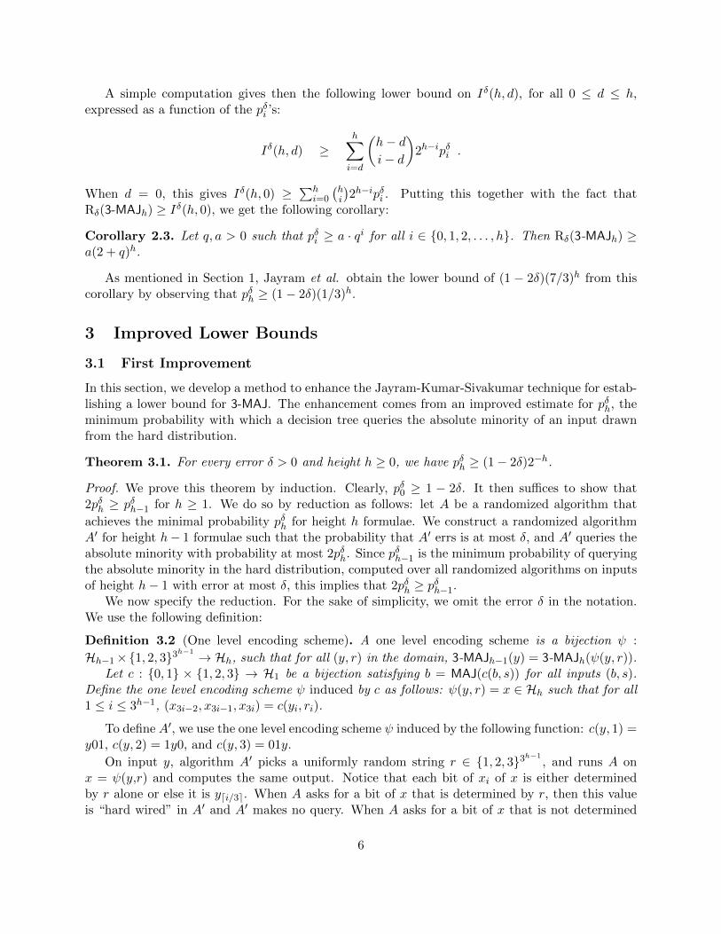
A simple computation gives then the following lower bound on Iδ(h, d), for all 0 ≤ d ≤ h,expressed as a function of the pδi ’s:

Iδ(h, d) ≥h∑i=d

(h− di− d

)2h−ipδi .

When d = 0, this gives Iδ(h, 0) ≥ ∑hi=0

(hi

)2h−ipδi . Putting this together with the fact that

Rδ(3-MAJh) ≥ Iδ(h, 0), we get the following corollary:

Corollary 2.3. Let q, a > 0 such that pδi ≥ a · qi for all i ∈ 0, 1, 2, . . . , h. Then Rδ(3-MAJh) ≥a(2 + q)h.

As mentioned in Section 1, Jayram et al. obtain the lower bound of (1 − 2δ)(7/3)h from thiscorollary by observing that pδh ≥ (1− 2δ)(1/3)h.

3 Improved Lower Bounds

3.1 First Improvement

In this section, we develop a method to enhance the Jayram-Kumar-Sivakumar technique for estab-lishing a lower bound for 3-MAJ. The enhancement comes from an improved estimate for pδh, theminimum probability with which a decision tree queries the absolute minority of an input drawnfrom the hard distribution.

Theorem 3.1. For every error δ > 0 and height h ≥ 0, we have pδh ≥ (1− 2δ)2−h.

Proof. We prove this theorem by induction. Clearly, pδ0 ≥ 1 − 2δ. It then suffices to show that2pδh ≥ pδh−1 for h ≥ 1. We do so by reduction as follows: let A be a randomized algorithm that

achieves the minimal probability pδh for height h formulae. We construct a randomized algorithmA′ for height h− 1 formulae such that the probability that A′ errs is at most δ, and A′ queries theabsolute minority with probability at most 2pδh. Since pδh−1 is the minimum probability of queryingthe absolute minority in the hard distribution, computed over all randomized algorithms on inputsof height h− 1 with error at most δ, this implies that 2pδh ≥ pδh−1.

We now specify the reduction. For the sake of simplicity, we omit the error δ in the notation.We use the following definition:

Definition 3.2 (One level encoding scheme). A one level encoding scheme is a bijection ψ :

Hh−1×1, 2, 33h−1 → Hh, such that for all (y, r) in the domain, 3-MAJh−1(y) = 3-MAJh(ψ(y, r)).

Let c : 0, 1 × 1, 2, 3 → H1 be a bijection satisfying b = MAJ(c(b, s)) for all inputs (b, s).Define the one level encoding scheme ψ induced by c as follows: ψ(y, r) = x ∈ Hh such that for all1 ≤ i ≤ 3h−1, (x3i−2, x3i−1, x3i) = c(yi, ri).

To define A′, we use the one level encoding scheme ψ induced by the following function: c(y, 1) =y01, c(y, 2) = 1y0, and c(y, 3) = 01y.

On input y, algorithm A′ picks a uniformly random string r ∈ 1, 2, 33h−1, and runs A on

x = ψ(y,r) and computes the same output. Notice that each bit of xi of x is either determinedby r alone or else it is ydi/3e. When A asks for a bit of x that is determined by r, then this valueis “hard wired” in A′ and A′ makes no query. When A asks for a bit of x that is not determined

6

by r, then and A′ queries the corresponding bit of y. Observe that A′ has error at most δ as3-MAJh−1(y) = 3-MAJh(ψ(y, r)) for all r, and A has error at most δ. We claim that

2 PrB∈RA, x∈RHh

[B(x) queries xm(x)] ≥ PrB∈RA, (y,r)∈RH′h

[B′(y, r) queries ym(y)] , (1)

whereH′h is the uniform distribution overHh−1×1, 2, 33h−1

and B′ is the algorithm that computesx = ψ(y, r) and then evaluates B(x). We prove this inequality by taking an appropriate partition ofthe probabilistic space of hard inputs Hh, and prove Eq. (1) separately, on each set in the partition.For h = 1, the two classes of the partition are H0

1 and H11 . For h > 1, the partition consists of the

equivalence classes of the relation ∼ defined by x ∼ x′ if xi = x′i for all i satisfying P (i) 6= P (m(x))in the tree T .

Because ψ is a bijection, observe that this also induces a partition of (y, r), where (y, r) ∼ (y′, r′)if and only if ψ(y, r) ∼ ψ(y′, r′). Also observe that every equivalence class contains three elements.Then Eq. (1) follows from the following stronger statement: for every equivalence class S, and forall B in the support of A, it holds that

2 Prx∈RHh

[B(x) queries xm(x) | x ∈ S] ≥ Pr(y,r)∈RH′h

[B′(y, r) queries ym(y) | ψ(y, r) ∈ S] . (2)

The same proof applies to all sets S, but to simplify the notation, we consider a set S thatsatisfies the following: for x ∈ S, we have m(x) ∈ 1, 2, 3 and xm(x) = 1. Observe that for eachj > 3, the jth bits of all three elements in S coincide. Therefore, the restriction of B to thevariables (x1, x2, x3), when looking only at the three inputs in S, is a well-defined decision tree onthree variables. We call this restriction C, and formally it is defined as follows: for each query xjmade by B for j > 3, C simply uses the value of xj that is shared by all x ∈ S and that we hard-wireinto C; for each query xj made by B where j ∈ 1, 2, 3, C actually queries xj . Note that therestriction C does not necessarily compute MAJ1(x1, x2, x3), for two reasons. Firstly, C is derivedfrom B, which may err on particular inputs. But even if B(x) correctly computes 3-MAJh(x), itmight happen that B never queries any of x1, x2, x3, or it might query one and never query a secondone, etc.

For any x ∈ S, recall that we write (y, r) the unique solution of ψ(y, r) = x. It holds for ourchoice of S that m(y) = 1 because we assumed m(x) ∈ 1, 2, 3 and also y1 = ym(y) = 0 becausewe assumed xm(x) = 1.

Observe that, for inputs x ∈ S, B queries xm(x) if and only if C queries the minority amongx1, x2, x3. Also, B′(y, r) queries ym(y) if and only if C(ψ(0, r1)) queries xr1 (cf. definition of c).Furthermore, the distribution of x1x2x3 when x ∈R S is uniform overH0

1. Similarly, the distributionof r1 over uniform (y, r) conditioned on ψ(y, r) ∈ S is identical to that of (0, r1) = ψ−1(x1x2x3) forx1x2x3 ∈R H0

1. Thus Eq. (2) is equivalent to:

Prx∈RH0

1

[C(x) queries xr1 where ψ(0, r1) = x] ≤ 2 Prx∈RH0

1

[C(x) queries xm(x)] . (3)

In principle, one can prove this inequality by considering all the (finitely many) decision treesC on three variables. We present here a somewhat more compact argument.

If C does not query any bit, both sides of Eq. (3) are zero, so the inequality holds. We thereforeassume that C makes at least one query and, without loss of generality, we also assume that thefirst query is x1. We distinguish two cases.

7

If C makes a second query when the first query is evaluated to 0 then the right hand side ofEq. (3) is at least 4/3 = 2 · (1/3 + 1/3) because there is a 1/3 chance that the first query is m(x)and 1/3 chance that the second is m(x). But the left hand side is at most 1, and therefore theinequality holds.

If C does not make a second query when the first query is evaluated to 0 then the left hand sideis at most 2/3 since for x = 010, we have r1 = 3, but x3 is not queried. With probability 1/3 wehave m(x) = 1, so the right hand side is at least 2/3. We conclude that Eq. (3) holds for every C.

We remark that the decision tree algorithm making no queries is not the only one that makesEq. (3) hold with equality. Another such algorithm is the following: first query x1, if x1 = 0, stop,else if x1 = 1, query x2 and stop.

To handle a general S, we replace 1, 2, 3 with m(x) and its two siblings. For S such thatx ∈ S satisfies xm(x) = 0, the optimal algorithm C ′ is the same as the one described above, exceptthat each 0 is changed to 1 and vice versa.

Therefore Eq. (3) holds for every C, which implies the theorem.

Combining Corollary 2.3 and Theorem 3.1, we obtain the following lower bound.

Corollary 3.3. Rδ(3-MAJh) ≥ (1− 2δ)(5/2)h.

3.2 Further Improvement

The proof of Theorem 3.1 proceeds by proving a recurrence, using a one level encoding scheme, forthe minimal probability pδh that an algorithm queries the absolute minority bit. It is natural to askwhether this is the best possible recurrence. In this section, we show that it is indeed possible toimprove the recurrence by using higher level encoding schemes.

In the following, we sometimes omit the error parameter δ from the notation in the interest of

readability. Let R = 0, 1 × 1, 2, 3, R(1)h = R3h−1

, and R(k)h = R(k−1)

h ×R3h−k .

Definition 3.4 (Uniform k-level encoding scheme). Let c : 0, 1 ×R → H1 be the function givenby c(y, (b, 1)) = yb(1− b), c(y, (b, 2)) = (1− b)yb, and c(y, (b, 3)) = b(1− b)y. The uniform k-levelencoding scheme ψ(k), for an integer k ≥ 1 is defined by the following recursion:

1. For h ≥ 1, y ∈ Hh−1 and r ∈ R(1)h we set ψ(1)(y, r) = x ∈ Hh such that (x3i−2, x3i−1, x3i) =

c(yi, ri), for all 1 ≤ i ≤ 3h−1;

2. for h ≥ k > 1, y ∈ Hh−k and (R, r) ∈ R(k)h we set ψ(k)(y, (R, r)) = ψ(k−1)(ψ(1)(y, r), R).

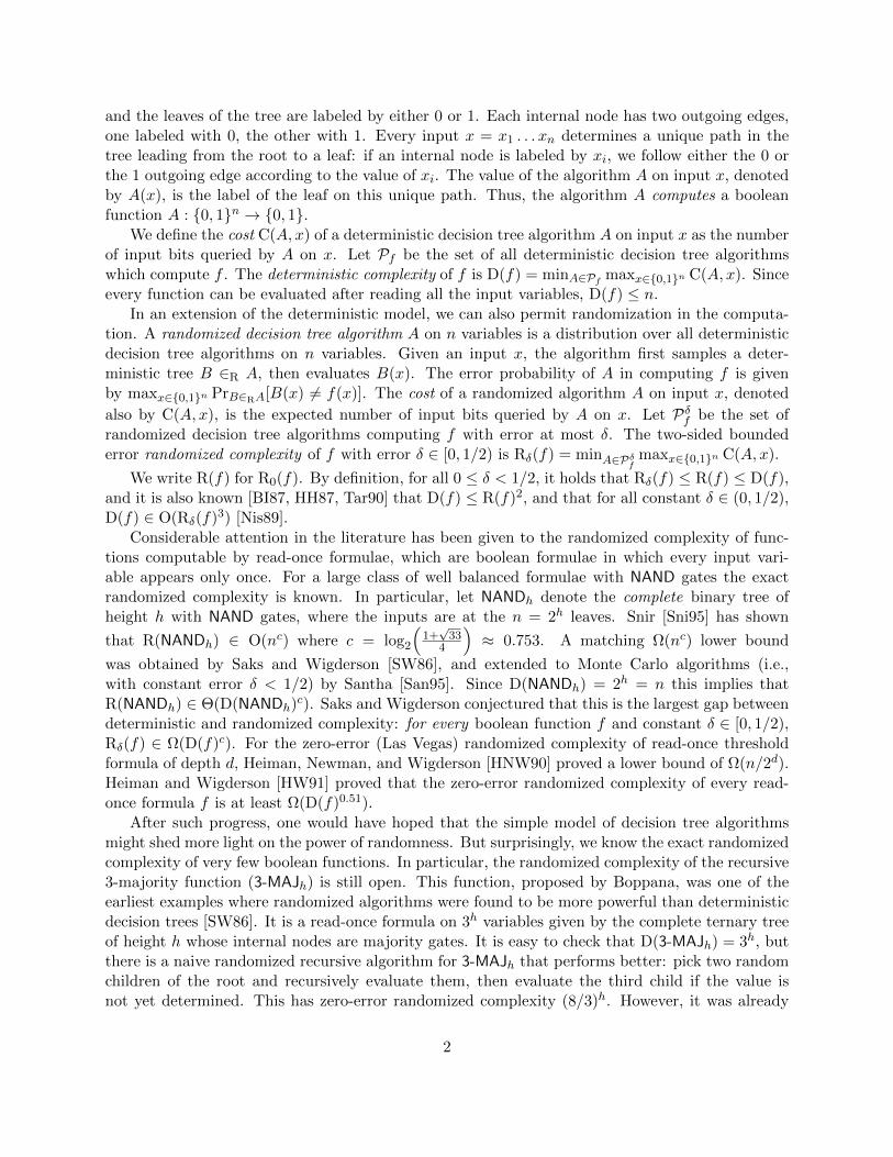
The uniform 2-level encoding scheme is illustrated in Figure 1. This encoding is no longer abijection. However, one can make essentially the same argument as Theorem 3.1. The advantageof this scheme over the one used earlier is the higher symmetry: while in the previous encoding,the instances in Hh are related by cyclic permutations of triples of three siblings, now the entiresymmetric group acts on them. Because of this higher symmetry if one of three siblings has beenqueried, the remaining two still play symmetric roles.

We later use the following observations that hold for all h ≥ k ≥ 1:

1. For all y ∈ Hh−k and r ∈ R(k)h we have 3-MAJh−k(y) = 3-MAJh(ψ(k)(y, r)).

8

b1 (1 ! b1) (1 ! b) (1 ! b2)b2y1

(1 ! b) y1

(1 ! b3)b3 b

b

y1

r = 2

r1 = 3 r2 = 1 r3 = 3

y1

x1 x2 x3 x4 x5 x6 x7 x8 x9

u v w

Figure 1: In a uniform 2-level encoding, a bit y1 is encoded as the height-2 recursive majorityof 9 bits x1x2 · · ·x9. On the right hand side, we give an example of the 9 bits with specific choicesof r, r1, r2, r3 for the two levels. In this example, when y1 = 0, then b3 encodes the absolute minoritybit if b = 1 and b3 = 0.

2. For (y, r) ∈R Hh−k ×R(k)h the value ψ(k)(y, r) is distributed uniformly in Hh.

3. For each r ∈ R(k)h and index i in the range 1 ≤ i ≤ 3h−k there is a unique index qi(r) in

the range (i − 1)3k + 1 ≤ qi(r) ≤ i3k such that for all y ∈ Hh−k we have xqi(r) = yi, where

x = ψ(k)h (y, r). If 1 ≤ j ≤ 3h but j is not equal to qi(r) for any i, then xj is independent of

the choice of y. We call these bits of x the fixed bits.

We use the uniform k-level encoding schemes to obtain better bounds on pδh. The argument isvery similar to the argument in Theorem 3.1. We start with proving a lower bound on pδh basedon a parameter computable by considering all the (finitely many) decision trees acting on inputsfrom H0

k. Then we proceed to computing this parameter. The high symmetry helps in reducingthe number of cases to be considered, but as k grows the length of the calculation increases ratherrapidly. We explain the basic structure of the calculation and also include a short Python programimplementing it in Appendix A. As an illustration, we do the calculation for k = 2 without the useof a computer. For k = 3, 4 we include the results of the program. A much more efficient algorithmwould be needed to make the calculation for k = 5 feasible.

Let us fix k ≥ 1 and let C be a deterministic decision tree algorithm on inputs of length 3k thatqueries at least one variable. We define

αC =Prx∈RH0

k,(y,r)∈Rψ−1(x)[C(x) queries xq1(r)]

Prx∈RH0k[C(x) queries xm(x)]

,

where ψ = ψ(k)k . Since C queries at least one bit, neither the numerator nor the denominator is

zero. So αC is well defined and positive. We emphasize that αC does not depend on the output ofC, it depends only on which input bits C queries. We further define

αk = maxC

αC ,

where the maximum extends over all deterministic decision trees C on 3k variables that query atleast one variable.

9

Theorem 3.5. For every k ≥ 1, h ≥ 0 integers and δ ≥ 0 real, we have

pδh ≥ (1− 2δ)(αk

2k

)α−h/kk .

Therefore,

Rδ(3-MAJh) ≥ (1− 2δ)(αk

2k

) (2 + α

−1/kk

)h.

Proof. We concentrate on the proof of the first statement; the second follows from Corollary 2.3.The proof follows the same structure as that of Theorem 3.1 but instead uses a depth-k recursion:

we show thatαk p

δh ≥ pδh−k (4)

if h ≥ k. To bound pδh in the base cases h < k, we invoke Theorem 3.1, i.e., pδh ≥ (1− 2δ)/2h, andthat αk ≤ 2k (from the proof of the theorem).

It remains to prove Eq. (4). We proceed as in Theorem 3.1: we consider a randomized δ-error algorithm A for 3-MAJh that achieves the minimum defining pδh and construct a randomizedalgorithm A′ for 3-MAJh−k with the same error that queries the absolute minority of a uniformlyrandom element of Hh−k with probability at most αk p

δh

To define A′, we use the uniform k-level encoding scheme ψ = ψ(k) (see Figure 1 for an illus-tration of the k = 2 case). On input y ∈ Hh−k the algorithm A′ picks a uniformly random element

r of R(k)h and simulates the decision tree A on input x = ψ(y, r). Whenever A queries a fixed

bit of x, the algorithm A′ makes no query, and when A queries a bit xqi(r), A′ queries yi. Define

H′h = Hh−k ×R(k)h . Then (y, r) ∈ H′h encodes ψ(y, r) ∈ Hh.

We partition Hh into equivalence classes, this time into sets of size 3l with l =∑k−1

i=0 3i. Forh = k, the two classes are H0

k and H1k. For h > k, an equivalence class consists of inputs that

are identical everywhere except in the height-k subtree containing their absolute minority. Moreformally, recall that P (i) denotes the parent of a node i in a tree, and let P (k) denote the k-foldcomposition of P with itself. In other words, P (k)(i) is the ancestor of the node i that is k levelsabove i. The partition of Hh for h > k consists of the equivalence classes of the relation defined asx ∼ x′ iff xi = x′i for all i satisfying P (k)(i) 6= P (k)(m(x)) in the tree Th.

Observe that the uniformity of the encoding implies that for every equivalence class S, and alldecision trees B in the support of A:

Prx∈RHh

[B(x) queries xm(x) | x ∈ S] = Pr(y,r)∈RH′h,x=ψ(y,r)

[B(x) queries xm(x) | x ∈ S] ,

and

Pr(y,r)∈RH′h

[B′(y, r) queries ym(y)|ψ(y, r) ∈ S] = Prx∈RHh,(y,r)∈Rψ−1(x)

[B′(y, r) queries ym(y)|x ∈ S] ,

where B′ is the algorithm that first computes x = ψ(y, r) and then evaluates B(x). We then provethat for every equivalence class S, and all B in the support of A, it holds that:

αk Prx∈RHh

[B(x) queries xm(x) | x ∈ S] ≥ Pr(y,r)∈RH′h

[B′(y, r) queries ym(y) | ψ(y, r) ∈ S] . (5)

Proving Eq. (5) for all B and S finishes the proof of the theorem.

10

Let us fix S and let z be the undetermined part of the input, i.e., the 3k variables in the height-ksubtree containing the absolute minority. Note that the set of possible values of z is either H0

k orH1k, depending on S. Now a deterministic decision tree B on inputs from S can be considered a

deterministic decision tree C for z. Indeed, the queries B asks outside z have a deterministic answerin S that can be hard wired in C. In case C asks no queries at all, then Eq. 5 is satisfied withzero on both sides of the inequality. Otherwise, if the possible values of z come from H0

k, Eq. (5)follows from αC ≤ αk (which, in turn, comes from the definition of αk as a maximum). Finally ifthe possible values of z are the 1-hard inputs, Eq. (5) is satisfied by symmetry.

To apply Theorem 3.5 we need to compute (or estimate) αk. For any fixed k this is a finitecomputation, but it is infeasible to do this by enumerating over all possible decision trees C over 3k

variables, even for small values of k.For a fixed integer k ≥ 1 and real α ≥ 0, we introduce a function ρα on decision trees on 3k

variables:

ρα(C) = Prx∈RH0

k,(y,r)∈Rψ−1(x)[C(x) queries xq1(r)]− α Pr

x∈RH0k

[C(x) queries xm(x)] . (6)

For the decision tree C0 not querying any variables we have ρα(C0) = 0, for other decision treesC we have ρα(C) > 0 if and only if αC > α. Thus, we have αk > α if and only if there exists Cwith ρα(C) > 0. Finding the maximum, i.e., maxC ρα(C) therefore answers the question whetherαk > α. We now focus on maximizing ρα for a given pair k, α. The advantage of this approachlies in the linearity of ρα, in a sense that we clarify below. This makes it easier to maximize ρα(C)than αC itself.

Let us call a bit of the hard input x ∈ Hk sensitive if the flipping of this input bit flips thevalue of 3-MAJk(x). Note that there are exactly 2k such bits for each hard input, these are theones where all nodes on the root to leaf path of the ternary tree evaluate to the same value.

Notice that for a fixed x ∈ H0k and (y, r) ∈R ψ−1(x) the position q1(r) (where the k-level

encoding ψ = ψ(k) “hides” the input variable y) is uniformly distributed over the 2k sensitivepositions. Thus, we can simplify Eq. (6) defining ρα as follows:

ρα(C) = 2−k πq(C)− απm(C) , (7)

where πq(C) is the expected number of sensitive bits queried by C(x) for x ∈R H0k and πm is the

probability that the absolute minority bit is queried by C for x ∈R H0k.

At any instant during the execution of a decision tree, we can partition the input variables intothose that have been queried and those that have not. We call the set of pairs (xi, ai) of variablesthat have already been queried, along with their values, the configuration of the decision tree atthat instant. The next action of the decision tree is either to stop (and produce an output that isnot relevant to this analysis) or to choose a variable that has not yet been queried, and query it. Inthe latter case, the configuration after the query is determined by the value of the chosen variable.

A decision tree is determined by the actions it takes in the possible configurations. In a config-uration γ, a decision tree that maximizes ρα takes an action that maximizes the linear combinationin Eq. (7) conditioned on reaching this configuration. Namely it maximizes

ρα(C, γ) = 2−k Pq(C, γ)− αPm(C, γ) , (8)

where Pq(C, γ) is the expected number of sensitive bits queried by C(x), when x is a uniformlyrandom 0-hard x consistent with γ, while Pm(C, γ) is the probability that C(x) queries the absolute

11

minority bit for a uniformly random 0-hard x consistent with γ. The optimal action in a configu-ration γ can therefore be found independently of the actions taken at configurations inconsistentwith γ. (A similar statement for the maximization of αC is false.)

Note that ρα(C, γ) is easy to compute if C stops at γ. If C queries a new variable at γ, thenρα(C, γ) is given by a convex combination of ρα(C, γ′) and ρα(C, γ′′), where γ′ and γ′′ are thetwo configurations resulting from the query. This leads to the following dynamic programmingalgorithm: consider all configurations in an order in which evaluating further variables yields con-figurations considered earlier. For each configuration γ we iterate through all actions to find anoptimal one and store the value of ρα(C, γ) for the optimal C. We have ρα(C) = ρα(C, ∅), where∅ is the initial configuration (in which no variable has been queried).

The number of all possible configurations is 33k. This makes the above algorithm infeasible

even for k = 3. We reduce the number of configurations considered significantly by appealing tosimple properties of 0-hard inputs:

1. We use the symmetries of the hard distribution. All the configurations γ in an orbit generatedby the automorphisms of the ternary tree give rise to the same value for ρα(C, γ). We consideronly one configuration in each such equivalence class.

2. We single out two types of configurations in which an optimal action is clear without the needfor further computation. First, if the configuration uniquely determines the value of the root(i.e., is not consistent with a 1-input), an optimal strategy is to stop. Second, if an unqueriedvariable is known not to be the absolute minority variable, querying it does not decrease theobjective function. We may thus assume that an optimal decision tree queries this variable.

We implement the second type of action as follows. The nodes in the path to the absoluteminority evaluate alternately to 0 and 1. If a node at odd depth evaluates to 0 or at evendepth evaluates to 1, then it is not on the absolute minority path. In this case, all variablesin the subtree rooted at the node are queried by an optimal decision tree. If a node at odddepth evaluates to 1, or at even depth evaluates to 0, then its siblings are not on the absoluteminority path. In this case, the variables in the subtrees rooted at the siblings are queried byan optimal decision tree.

We call a configuration γ unstable if there is an action that an optimal decision tree may takein γ as described in point 2. We call the configuration stable otherwise. Note that the value of theroot is not uniquely determined by a stable configuration. It suffices to store ρα(C, γ) for stable γ.If ρα(C, γ) is needed for some unstable configuration γ we apply the above rules (possibly multipletimes) until the value of the root is determined, or we arrive at a stable configuration. We thencompute ρα(C, γ) using the appropriate stored values.

The lone stable configuration for height 0 is ∅, the one in which the input variable has not beenqueried. Consider a stable configuration for height-k formulae, for k ≥ 1, and the restrictions ofthe configuration to the subtrees rooted at the three children of the root. Call the configurationobtained by negating the values of the variables in a configuration its dual . It is straightforward toverify that either a restriction uniquely determines the value of the corresponding child, or it is adual of a stable configuration for height (k− 1). No child of the root can be known to have value 1in a stable configuration and at most one of them can be known to have value 0. So an equivalenceclass of stable configurations for height k is determined by a multiset of (equivalence classes of)stable configurations for height (k − 1) of size 2 (when one child is known to have value 0) or of

12

size 3 (when the values of the children are all undetermined). This characterization gives us thefollowing recurrence relation for Nk, the number of equivalence classes of stable configurations forheight k:

Nk =

(Nk−1 + 1

2

)+

(Nk−1 + 2

3

),

with the initial condition N0 = 1. The recurrence gives us

N1 = 2

N2 = 7

N3 = 112

N4 = 246, 792 and

N5 = 2, 505, 258, 478, 767, 772 .

This makes the dynamic programming approach for optimizing ρα(C) feasible for k ≤ 4. Thisapproach is implemented by the Python program presented in Appendix A. In order to avoiddealing with dual configurations, the Python program considers NOT-3-MAJ, the recursive negatedmajority-of-three function. This is the function computed by the a negated majority gate in everyinternal node of a complete ternary tree.

Recall that using an algorithm to maximize ρα(C) we can check whether αk > α. Instead ofa binary search we find the exact value of αk as follows. With little modification, the algorithmwe present for maximizing ρα(C) also produces the value αC∗ for the optimal decision tree C∗.We then start with an arbitrary α ≤ αk, and repeatedly optimize ρα updating the estimate α tothe last value αC∗ , until we find that maxC ρα(C) = 0. This heuristic finds the maximum αk ina finite number of iterations. Instead of bounding the number of iterations in general we mentionthat starting from the initial value α = 0 the heuristic gives us αk in at most four iterations whenk = 2, 3, 4. The computations show:

α1 = 2 ,

α2 =24

7,

α3 =12231

2203, and

α4 =2027349

216164.

Using the value of α4, Theorem 3.5 yields the following bound.

Corollary 3.6.

Rδ(3-MAJh) ≥ (1/2− δ)(

2 +

(216164

2027349

)1/4)h

> (1/2− δ)2.57143h .

3.3 Analysis of the 2-level encoding

As an illustration of the use of higher level encodings we explicitly derive a second order recurrencefor pδh using 2-level encodings. We fix k = 2 and consider deterministic decision trees C on 9variables. We run these decision trees on inputs from H0

2.

13

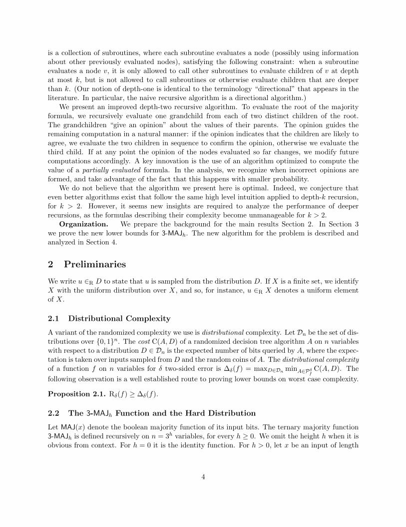
From the proof of Theorem 3.1, we have αC ≤ 4 for all C. We may verify that αC0 = 3 for thedecision tree C0 with the following strategy: first query x1, if x1 = 1, stop, else if x1 = 0, queryx2 and x3; then if MAJ(x1, x2, x3) = 0, stop, else query all remaining bits and stop. These boundsshow that 3 ≤ α2 ≤ 4, so it suffices to consider ρα for the values of α in the range [3, 4]. We provebelow that for these values of α a single decision tree C ′ maximizes ρα(C) among the deterministicdecision trees that query at least one variable. This decision tree C ′ is given in Figure 2. We statethe optimality of C ′ in the following lemma.

Lemma 3.7. Let C be any deterministic decision tree on 9-bit inputs that makes at least one queryand let C ′ be the decision tree depicted in Figure 2. Then for all α ∈ [3, 4], ρα(C) ≤ ρα(C ′).

Proof. Recall that the action in a configuration γ of the decision tree C that maximizes ρα(C) isthe one that maximizes ρα(C, γ) = 2−2Pq(C, γ)− αPm(C, γ). To simplify notation, we write ρ, Pqand Pm for ρα(C, γ), Pq(C, γ), and Pm(C, γ), respectively, if the decision tree C and configurationγ considered are clear from the context.

We call any set of 3 sibling nodes a clause, so that 1, 2, 3, 4, 5, 6 and 7, 8, 9 are clauses.We say a clause is evaluated if its majority is uniquely determined by the configuration underconsideration.

We argue that an algorithm that maximizes ρα(C) takes certain actions, without loss of gener-ality. We begin with three rules that are special cases of the general rules from Section 3.2 that weused to reduce the number of configurations considered.

1. If a bit is evaluated to 0, then evaluate all remaining bits in its clause.

2. If two bits in a clause are evaluated to 1 (this is the minority clause), evaluate all remainingbits in the other clauses.

3. if two clauses have been evaluated to 0, then stop.

In what follows we systematically consider all stable configurations for height 2 inputs, i.e., theones in which the above three rules do not apply. For each such configuration, we determine whataction(s) an optimal decision may take next, without loss of generality, in order to maximize ρα.

4. A single majority (0) clause is evaluated and either no variables are evaluated in either of theother clauses or a single 1 is evaluated in both the other clauses. In this case, stopping is thebest strategy. Indeed, m(x) has not been queried yet. Therefore if we stop, then Pm = 0 andPq = 2. This gives ρ = 1/2. But if C continues by querying at least one more bit, then Pm ≥1/6 or Pm ≥ 1/4 (since there are either 6 or 4 remaining unqueried variables, respectively,and they are symmetric) and Pq ≤ 4. Therefore, ρ = 2−2Pq − αPm ≤ 1 − α/6 ≤ 1/2 sinceα ≥ 3.

5. A single majority clause is evaluated and one more bit is evaluated to 1, but nothing more.There are 9 inputs consistent with this configuration. We argue that stopping is best, asin the previous case. The argument is more involved because there is no global symmetrybetween the unqueried variables. We separately compare stopping with querying a variableinside or outside the untouched clause.

If we stop, then Pq = 2 and Pm = 0, so we have ρ = 1/2.

14

If we query a variable in the clause containing the evaluated bit 1, then there are 3 consistentinputs in which the next queried bit is m(x). So we have Pm ≥ 1/3 and Pq ≤ 4. Since α ≥ 3,ρ ≤ 0.

If we query a variable in the untouched clause, then there is 1 out of the 9 consistent inputsfor which this next queried variable is m(x), making Pm ≥ 1/9. There are 4 more consistentinputs for which this variable evaluates to 1. In this case we arrive at the configurationcovered by item 4 above. Using that rule, the algorithm stops, leaving 2 out the 4 sensitivebits unqueried. Thus, we have Pq ≤ 4− 4/9 · 2 = 28/9 and ρ ≤ 4/9, which is lesser than the1/2 obtained if we stop.

6. A single 1 has been evaluated in each of the three clauses and no other bit has been queried.In this case reading another bit is the best strategy (the choice of which bit is unimportantbecause of symmetry). Observe that no bit 0 has been evaluated yet. Therefore if C stops,we have ρ = Pq = Pm = 0. If C continues to query another bit, which bit it queries doesnot matter by symmetry. Then the rest of the algorithm is determined by the earlier rulesyielding Pq = 8/3, Pm = 1/6, and ρ = 2/3− α/6 ≥ 0.

7. A single bit 1 has been evaluated in each of two different clauses and the third clause isuntouched. Then it is best to evaluate a bit of the third clause. If C stops we have ρ = Pm =Pq = 0.

If C reads another bit in one of the clauses containing a single 1 bit, then the rest of thedecision tree algorithm is determined by the earlier rules and we get Pq = 14/5 and Pm = 1/5with ρ = 7/10− α/5. Note that whether this option is better than stopping depends on thevalue of α.

If C reads a bit in the untouched clause, then by using the rules already presented in theprevious cases, we calculate Pq = 12/5 and Pm = 2/15, yielding ρ = 3/5 − 2α/15. This ismore than both 0 and 7/10− α/5 in the entire range of α we are considering.

8. A single bit 1 has been evaluated in one clause and no other clauses are touched. Then it isbest to evaluate a bit of another clause. If C stops, then we have ρ = Pm = Pq = 0.

If C evaluates another bit in the clause containing 1, then the rest of C is determined byearlier rules and we have Pq = 3, Pm = 1/4 and ρ = 3/4− α/4 ≤ 0.

But if C queries a bit in an untouched clause, then similar calculations yield Pq = 7/3,Pm = 5/36 and ρ = 7/12− 5α/36 > 0, making this the best choice.

Following all the above rules and always choosing the smallest index when symmetry allowsus to choose, we arrive at a well defined decision tree, namely C ′. This finishes the proof of thelemma.

The above lemma immediately gives us the value of α2.

Theorem 3.8. α2 = 24/7.

Proof. As observed in the paragraph before Lemma 3.7 we have 3 ≤ α2 ≤ 4. By the lemma weknow that ρα(C) in this range is maximized by either C ′ or the decision tree that does not queryany variable. The latter gives ρα = 0. We have α ≥ α2 if and only if this maximum is 0, so

15

x1

x2, x3

Stop All

(1 ! !)/92/9Stop All

Stop All

0

x4

x7

x2

x3

x8, x9

x5, x6

All but x3

Stop All

1

1, 10, 11

0, 1 1, 1

(1 ! !)/271/9

0

1 0

0, 1 1, 1

4/81 (1 ! !)/81

01

10

(1 ! !)/812/81

1/81

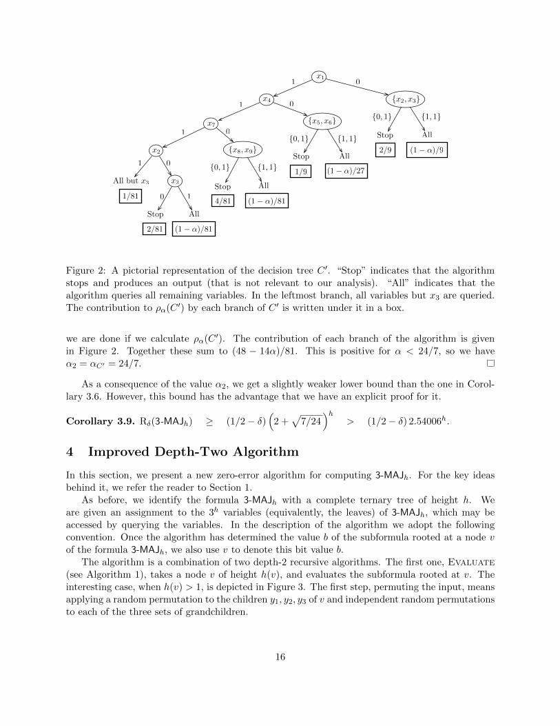
Figure 2: A pictorial representation of the decision tree C ′. “Stop” indicates that the algorithmstops and produces an output (that is not relevant to our analysis). “All” indicates that thealgorithm queries all remaining variables. In the leftmost branch, all variables but x3 are queried.The contribution to ρα(C ′) by each branch of C ′ is written under it in a box.

we are done if we calculate ρα(C ′). The contribution of each branch of the algorithm is givenin Figure 2. Together these sum to (48 − 14α)/81. This is positive for α < 24/7, so we haveα2 = αC′ = 24/7.

As a consequence of the value α2, we get a slightly weaker lower bound than the one in Corol-lary 3.6. However, this bound has the advantage that we have an explicit proof for it.

Corollary 3.9. Rδ(3-MAJh) ≥ (1/2− δ)(

2 +√

7/24)h

> (1/2− δ) 2.54006h.

4 Improved Depth-Two Algorithm

In this section, we present a new zero-error algorithm for computing 3-MAJh. For the key ideasbehind it, we refer the reader to Section 1.

As before, we identify the formula 3-MAJh with a complete ternary tree of height h. Weare given an assignment to the 3h variables (equivalently, the leaves) of 3-MAJh, which may beaccessed by querying the variables. In the description of the algorithm we adopt the followingconvention. Once the algorithm has determined the value b of the subformula rooted at a node vof the formula 3-MAJh, we also use v to denote this bit value b.

The algorithm is a combination of two depth-2 recursive algorithms. The first one, Evaluate(see Algorithm 1), takes a node v of height h(v), and evaluates the subformula rooted at v. Theinteresting case, when h(v) > 1, is depicted in Figure 3. The first step, permuting the input, meansapplying a random permutation to the children y1, y2, y3 of v and independent random permutationsto each of the three sets of grandchildren.

16

Algorithm 1 Evaluate(v): evaluate a node v.

Input: Node v with subtree of height h(v).Output: the bit value 3-MAJh(Z(v)) of the subformula rooted at v

Let h = h(v)

if h = 0 then . First base case: h = 0 (v is a leaf)Query Z(v) to get its value a; return a

end if

Let y1, y2, y3 be a uniformly random permutation of the children of v . v has height h ≥ 1

if h = 1 then . Second base case: h = 1Evaluate(y1) and Evaluate(y2)if y1 = y2 then return y1else return Evaluate(y3)end if

end if. Recursive case: v has height h ≥ 2; use the attached figure as a guide

Let x1 and x2 be chosen uniformly at random from the children of y1 and y2, respectively

v

y1 y2 y3

x1 x2

Evaluate(x1) and Evaluate(x2)

if x1 6= x2 thenEvaluate(y3)Let b ∈ 1, 2 be such that xb = y3Complete(yb, xb)if yb = y3 then return ybelse return Complete(y3−b, x3−b)end if

else [x1 = x2]Complete(y1, x1)if y1 = x1 then

Complete(y2, x2)if y2 = y1 then return y1else [y2 6= y1] return Evaluate(y3)end if

else [y1 6= x1]Evaluate(y3)if y3 = y1 then return y1else return Complete(y2, x2)end if

end ifend if

17

E(x1), E(x2)

x1 = x2

x1 != x2

C(y1, x1)

E(y3)

y1 = x2

C(y2, x2)

y2 = y1

Output y1

E(y3) Output y3

y2 != y1

E(y3) Output y3

Output y2

y1 != x2

y3 = y1

y3 != y1

C(y2, x2)

such that y3 = yb

Set b ! 1, 2

Permute input

C(yb, xb)

yb = y3

yb != y3

Output y3

Output MAJ(y1, y2, y3)C(y3!b, x3!b)

v

y1 y2 y3

x1 x2

Figure 3: Pictorial representation of algorithm Evaluate on a subformula of height h(v) ≥ 2rooted at v. It is abbreviated by the letter ‘E’ when called recursively on descendants of v. Theletter ‘C’ abbreviates the second algorithm Complete depicted in Figure 4.

18

The second algorithm, Complete (see Algorithm 2), is depicted in Figure 4. It takes twoarguments v, y1, and completes the evaluation of the subformula 3-MAJh rooted at node v,where h(v) ≥ 1, and y1 is a child of v whose value has already been evaluated. The first step,permuting the input, means applying a random permutation to the children y2, y3 of v and inde-pendent random permutations to each of the two sets of grandchildren of y2, y3. Note that this issimilar in form to the depth 2 algorithm due to [JKS03].

Algorithm 2 Complete(v, y1): finish the evaluation of the subformula rooted at node v

Input: Node v of height h(v); child y1 of v which has already been evaluatedOutput: the bit value 3-MAJh(Z(v))

Let h = h(v)

Let y2, y3 be a uniformly random permutation of the two children of v other than y1

if h = 1 then . Base caseEvaluate(y2)if y2 = y1 then return y1else return Evaluate(y3)end if

end if

Let x2 be chosen uniformly at random from the children of y2 . Recursive case. use the attached figure as a guide

v

y1 y2 y3

x2

Evaluate(x2)

if y1 6= x2 thenEvaluate(y3)if y1 = y3 then return y1else return Complete(y2, x2)end if

else [y1 = x2]Complete(y2, x2)if y1 = y2 then return y1else return Evaluate(y3)end if

end if

To evaluate an input of height h, we invoke Evaluate(r), where r is the root. The correctnessof the two algorithms follows by inspection—they determine the values of as many children of thenode v as is required to compute the value of v.

For the complexity analysis, we study the expected number of queries they make for a worst-case input of fixed height h. (A priori , we do not know if such an input is a hard input as definedin Section 2.2.) Let T (h) be the worst-case complexity of Evaluate(v) for v of height h. ForComplete(v, y1), we distinguish between two cases. Let y1 be the child of node v that has alreadybeen evaluated. The complexity given that y1 is the minority child of v is denoted by Sm, and thecomplexity given that it is a majority child is denoted by SM.

The heart of the analysis is the following set of recurrences that relate T, SM and Sm to eachother.

Lemma 4.1. We have Sm(1) = 2, SM(1) = 32 , T (0) = 1, and T (1) = 8

3 .

19

C(y2, x2)

y2 = y1

Output y1

E(y3) Output y3

y2 != y1

E(y3) Output y3

Output y2

y3 = y1

y3 != y1

C(y2, x2)

Permute input

v

y1 y2 y3

x2

E(x2)

x2 = y1

x2 != y1

Figure 4: Pictorial representation of algorithm Complete on a subformula of height h ≥ 1 rootedat v one child y1 of which has already been evaluated. It is abbreviated by the letter ‘C’ whencalled recursively on descendants of v. Calls to Evaluate are denoted ‘E’.

For all h ≥ 1, it holds that

SM(h) ≤ Sm(h) and SM(h) ≤ T (h) . (9)

Finally, for all h ≥ 2, it holds that

Sm(h) = T (h− 2) + T (h− 1) +2

3SM(h− 1) +

1

3Sm(h− 1) , (10)

SM(h) = T (h− 2) +2

3T (h− 1) +

1

3SM(h− 1) +

1

3Sm(h− 1) , and (11)

T (h) = 2T (h− 2) +23

27T (h− 1) +

26

27SM(h− 1) +

18

27Sm(h− 1) . (12)

Proof. We prove these relations by induction. The bounds for h ∈ 0, 1 follow immediately byinspection of the algorithms. To prove the statement for h ≥ 2, we assume the recurrences hold forall l < h. Observe that it suffices to prove Equations (10), (11), (12) for height h, since the valuesof the coefficients immediately imply that Inequalities (9) holds for h as well.

Equation (10). Since Complete(v, y1) always starts by computing the value of a grand-child x2 of v, we get the first term T (h − 2) in Eq. (10). It remains to show that the worst-casecomplexity of the remaining queries is T (h− 1) + (2/3)SM(h− 1) + (1/3)Sm(h− 1).

Since y1 is the minority child of v, we have that y1 6= y2 = y3. The complexity of the remainingsteps is summarized in the next table in the case that the three children of node y2 are not allequal. In each line of the table, the worst case complexity is computed given the event in the firstcell of the line. The second cell in the line is the probability of the event in the first cell over therandom permutation of the children of y2. This gives a contribution of T (h − 1) + (2/3)SM(h −1) + (1/3)Sm(h− 1).

20

Sm(h) (we have y1 6= y2 = y3)

event probability complexity

y2 = x2 2/3 T (h− 1) + SM(h− 1)

y2 6= x2 1/3 T (h− 1) + Sm(h− 1)

This table corresponds to the worst case, as the only other case is when all children of y2 areequal, in which the cost is T (h−1) +SM(h−1). Applying Inequality (9) for h−1, this is a smallercontribution than the case where the children are not all equal.

Therefore the worst case complexity for Sm is given by Eq. (10). We follow the same conventionand appeal to this kind of argument also while deriving the other two recurrence relations.

Equation (11). Since Complete(v, y1) always starts by computing the value of a grand-child x2 of v, we get the first term T (h − 2) in Eq. (11). There are then two possible patterns,depending on whether the three children y1, y2, y3 of v are all equal. If y1 = y2 = y3, we have inthe case that all children of y2 are not equal that:

SM(h) if y1 = y2 = y3event probability complexity

y2 = x2 2/3 SM(h− 1)

y2 6= x2 1/3 T (h− 1)

As in the above analysis of Eq. (10), applying Inequalities (9) for height h − 1 we get that thecomplexity in the case when all children of y2 are equal is bounded above by the complexity whenthe children are not all equal. Therefore the above table describes the worst-case complexity forthe case when y1 = y2 = y3.

If y1, y2, y3 are not all equal, we have two events y1 = y2 6= y3 or y1 = y3 6= y2 of equalprobability as y1 is a majority child of v. This leads to the following tables for the case where thechildren of y2 are not all equal

SM(h) given y1 = y2 6= y3event prob. complexity

y2 = x2 2/3 SM(h− 1)

y2 6= x2 1/3 T (h− 1) + Sm(h− 1)

SM(h) given y1 = y3 6= y2event prob. complexity

y2 = x2 2/3 T (h− 1)

y2 6= x2 1/3 T (h− 1) + Sm(h− 1)

As before, we apply Inequalities (9) for height h − 1 to see that the worst case occurs when thechildren of y2 are not all equal.

From the above tables, we deduce that the worst-case complexity occurs on inputs wherey1, y2, y3 are not all equal. This is because Inequalities (9) for height h− 1 imply that, line by line,the complexities in the table for the case y1 = y2 = y3 are upper bounded by the correspondingentries in each of the latter two tables. To conclude Eq. (11), recall that the two events y1 = y2 6= y3and y1 = y3 6= y2 occur with probability 1/2 each:

SM(h) = T (h− 2) +1

2

[2

3SM(h− 1) +

1

3(T (h− 1) + Sm(h− 1))

]+

1

2

[2

3T (h− 1) +

1

3(T (h− 1) + Sm(h− 1))

].

Equation (12). Since Evaluate(v) starts with two calls to itself to compute x1, x2, we getthe first term 2T (h− 2) on the right hand side. For the remaining terms, we consider two possible

21

cases, depending on whether the three children y1, y2, y3 of v are equal. If y1 = y2 = y3, assumingthat the children of y1 are not all equal, and the same for the children of y2, we have

T (h) given y1 = y2 = y3event probability complexity

y1 = x1, y2 = x2 4/9 2SM(h− 1)

y1 = x1, y2 6= x2 2/9 T (h− 1) + SM(h− 1)

y1 6= x1, y2 = x2 2/9 T (h− 1) + SM(h− 1)

y1 6= x1, y2 6= x2 1/9 T (h− 1) + Sm(h− 1)

As before, the complexities are in non-decreasing order, and we observe that Inequalities (9) forheight h−1 imply that in a worst case input the children of y1 are not all equal, and that the sameholds for the children of y2.

If y1, y2, y3 are not all equal, we have three events y1 = y2 6= y3, y1 6= y2 = y3 and y3 = y1 6= y2each of which occurs with probability 1/3. This leads to the following analyses

T (h) given y1 = y2 6= y3event probability complexity

y1 = x1, y2 = x2 4/9 2SM(h− 1)

y1 = x1, y2 6= x2 2/9 T (h− 1) + SM(h− 1) + Sm(h− 1)

y1 6= x1, y2 = x2 2/9 T (h− 1) + SM(h− 1) + Sm(h− 1)

y1 6= x1, y2 6= x2 1/9 T (h− 1) + 2Sm(h− 1)

T (h) given y1 6= y2 = y3event probability complexity

y1 = x1, y2 = x2 4/9 T (h− 1) + SM(h− 1)

y1 = x1, y2 6= x2 2/9 T (h− 1) + SM(h− 1) + Sm(h− 1)

y1 6= x1, y2 = x2 2/9 T (h− 1) + SM(h− 1) + Sm(h− 1)

y1 6= x1, y2 6= x2 1/9 T (h− 1) + 2Sm(h− 1)

T (h) given y3 = y1 6= y2event probability complexity

y1 = x1, y2 = x2 4/9 T (h− 1) + SM(h− 1)

y1 = x1, y2 6= x2 2/9 T (h− 1) + SM(h− 1) + Sm(h− 1)

y1 6= x1, y2 = x2 2/9 T (h− 1) + Sm(h− 1)

y1 6= x1, y2 6= x2 1/9 T (h− 1) + 2Sm(h− 1)

In all three events, we observe that Inequalities (9) for height h − 1 imply that in a worst caseinput, the children of y1 are not all equal, and the same holds for the children of y2.

Applying Inequalities (9) for height h − 1, it follows that line by line the complexities in thelast three tables are at least the complexities in the table for the case y1 = y2 = y3. Therefore theworst case also corresponds to an input in which y1, y2, y3 are not all equal. We conclude Eq. (12)as before, by taking the expectation of the complexities in the last three tables.

Theorem 4.2. T (h), SM(h), and Sm(h) are all in O(αh), where α ≤ 2.64944.

Proof. We make an ansatz T (h) ≤ aαh, SM(h) ≤ b αh, and Sm(h) ≤ c αh, and find con-stants a, b, c, α for which we may prove these inequalities by induction.

22

The base cases tell us that 2 ≤ cα, 32 ≤ bα, 1 ≤ a, and 8

3 ≤ aα.Assuming we have constants that satisfy these conditions, and that the inequalities hold for

all appropriate l < h, for some h ≥ 2, we derive sufficient conditions for the inductive step to gothrough.

By the induction hypothesis, Lemma 4.1, and the ansatz, we have

Sm(h) ≤ aαh−2 + aαh−1 +2b

3αh−1 +

c

3αh−1 ,

SM(h) ≤ aαh−2 +2a

3αh−1 +

b

3αh−1 +

c

3αh−1 , and

T (h) ≤ 2aαh−2 +23a

27αh−1 +

26

27αh−1 +

18

27αh−1 .

These would imply the required bounds on Sm(h), SM(h), T (h) if

a+ 3a+2b+c3 α ≤ c α2 , a+ 2a+b+c

3 α ≤ b α2 , and 2a+ 23a+26b+18c27 α ≤ aα2 . (13)

The choice α = 2.64944, a = 1.02, b = 0.559576× a, and c = 0.755791× a satisfies the base case aswell as all the Inequalities (13), so the theorem holds by induction.

5 Concluding remarks

In this article, we revisited a technique due to Jayram, Kumar, and Sivakumar for proving alower bound on the decision tree complexity of 3-MAJh, the recursive majority-of-three function ofheight h. We showed that it could be enhanced by obtaining better estimates on the probability pδhwith which the absolute minority variable is queried under the hard distribution. The new estimatesare obtained by considering highly symmetric encodings of height-(h−k) inputs into height-h inputs.The analysis of the encodings quickly becomes intractable with growing k. However, by appealingto the underlying symmetry in the function, the analysis can be executed explicitly for k = 1, 2,and with the aid of a computer for k ≤ 4. This leaves us with several immediate questions aboutthe technique:

1. Is there is a more efficient algorithm for the analysis?

2. Is there a succinct, explicit analysis for larger values of k?

3. What is the best lower bound we can obtain using this technique?

4. Does this technique give us any intuition into more efficient algorithms?

We also present a new (more efficient) algorithm for 3-MAJh based on the idea that a partialevaluation of a formula helps us form an opinion about the value of its subformulae. We use theopinions at a certain stage of the algorithm to choose the next variable to query. Additionally, weuse a depth-2 recursive algorithm that is optimized for computing the value of a partially evaluatedformula. It is likely that algorithms with depth k recursion, with k > 2 give us further improvementsin efficiency. However, their analysis seems to be beyond the scope of the techniques used in thiswork.

23

References

[BI87] M. Blum and R. Impagliazzo. General oracle and oracle classes. In Proceedings of 28thIEEE Symposium on Foundations of Computer Science, pages 118–126, 1987.

[HH87] J. Hartmanis and L. Hemachandra. One-way functions, robustness, and non-isomorphism of NP-complete sets. In Proceedings of 2nd Structure in Complexity TheoryConference, pages 160–173, 1987.

[HNW90] R. Heiman, I. Newman, and A. Wigderson. On read-once threshold formulae and theirrandomized decision tree complexity. In Proceedings of 5th Structure in ComplexityTheory, pages 78–87, 1990.

[HW91] R. Heiman and A. Wigderson. Randomized versus deterministic decision tree complexityfor read-once boolean functions. In Proceedings of 6th Structure in Complexity TheoryConference, pages 172–179, 1991.

[JKS03] T. Jayram, Ravi Kumar, and D. Sivakumar. Two applications of information complex-ity. In Proceedings of 35th ACM Symposium on Theory of Computing, pages 673–682,2003.

[Leo13] Nikos Leonardos. An improved lower bound for the randomized decision tree complexityof recursive majority. In Fedor V. Fomin, Rusins Freivalds, Marta Z. Kwiatkowska,and David Peleg, editors, Proceedings of 40th International Colloquium on Automata,Languages and Programming, volume 7965 of Lecture Notes in Computer Science, pages696–708. Springer, 2013.

[LNPV06] I. Landau, A. Nachmias, Y. Peres, and S. Vanniasegaram. The lower bound forevaluating a recursive ternary majority function: an entropy-free proof. Techni-cal report, Department of Statistics, University of California, Berkeley, CA, USA,http://www.stat.berkeley.edu/110, 2006. Undergraduate Research Report.

[MNSX11] F. Magniez, A. Nayak, M. Santha, and D. Xiao. Improved bounds for the randomizeddecision tree complexity of recursive majority. In Proceedings of 38th InternationalColloquium on Automata, Languages and Programming, pages 317–329, 2011.

[Nis89] N. Nisan. CREW PRAMs and decision trees. In Proceedings of 21st Annual ACMSymposium on Theory of Computing, pages 327–335, 1989.

[RS08] B. Reichardt and Spalek. Span-program-based quantum algorithm for evaluating formu-las. In Proceedings of 40th ACM Symposium on Theory of Computing, pages 103–112,2008.

[San95] M. Santha. On the Monte Carlo boolean decision tree complexity of read-once formulae.Random Structures and Algorithms, 6(1):75–87, 1995.

[Sni95] M. Snir. Lower bounds for probabilistic linear decision trees. Theoretical ComputerScience, 38:69–82, 1995.

24

[SW86] M. Saks and A. Wigderson. Probabilistic boolean decision trees and the complexity ofevaluating game trees. In Proceedings of 27th Annual Symposium on Foundations ofComputer Science, pages 29–38, 1986.

[Tar90] G. Tardos. Query complexity or why is it difficult to separate NPA ∩ coNPA from PA

by a random oracle. Combinatorica, 9:385–392, 1990.

A Python program

The following Python program is also available at:https://www.dropbox.com/s/wcrdoib5h918p2e/commented-majority.py

def prep ( dep ) :global depth , g , d# depth = depth o f r e c u r s i v e NOT−3−MAJ c i r c u i t s cons idered# g [ i ] = l i s t o f depth i s t a b l e c o n f i g u r a t i o n s f o r 0 <= i <= depth# f o r a record r r e p r e s e n t i n g a c o n f i g u r a t i o n o f depth i# r [ 0 ] = # of e v a l u a t i o n s g i v i n g 0# r [ 1 ] = # of e v a l u a t i o n s g i v i n g 1# r [ 2 ] = # of q u e r i e d s e n s i t i v e b i t s in a l l e v a l u a t i o n s wi th c o r r e c t output# r [ 3 : 6 ] = i n d i c e s o f the t h r e e c h i l d r e n , s o r t e d ( where a p p l i c a b l e )# d [ i ] = d i c t i o n a r y t h a t t e l l s the index o f a s t a b l e c o n f i g u r a t i o n o f depth

i from the i n d i c e s o f i t s 3 depth i−1 c h i l d r e n# prep s e t s the v a l u e s o f t h e s e g l o b a l v a r i a b l e s ( w i l l not be changed )depth=depg = [ [ [ 0 , 1 , depth % 2 ] , [ 1 , 1 , 0 ] ] ]# two s t a b l e c o n f i g u r a t i o n s in g [ 0 ] : a v a r i a b l e s e t to 1 and a not q u e r i e d

v a r i a b l ed=[ ]# empty d i c t i o n a r y in d [ 0 ]for i in range (1 , depth+1) :

# b u i l d i n g g [ i ] and d [ i ] under the names gg and ddg l=g [−1]gg = [ [ 0 , 1 , ( ( depth−i )%2)∗2∗∗ i ] ]# the f i r s t record r e p r e s e n t s a f u l l y q u e r i e d s u b t r e e o f depth i

e v a l u a t i n g to 1dd=for a in range ( l en ( g l ) ) :

for b in range (max(a , 1 ) , l en ( g l ) ) :for c in range (b , l en ( g l ) ) :

# e n f o r c i n g a <= b <= c and no two f u l l y e v a l u a t e d s i b l i n g s in as t a b l e c o n f i g u r a t i o n

dd [ ( a , b , c ) ]= l en ( gg )A,B,C=g l [ a ] , g l [ b ] , g l [ c ]gg . append ( [A[ 0 ] ∗B[ 1 ] ∗C[1]+A[ 1 ] ∗B[ 0 ] ∗C[1]+A[ 1 ] ∗B[ 1 ] ∗C[ 0 ] ,A[ 1 ] ∗B[ 0 ] ∗C

[0]+A[ 0 ] ∗B[ 1 ] ∗C[0]+A[ 0 ] ∗B[ 0 ] ∗C[ 1 ] ,A[ 0 ] ∗B[ 1 ] ∗C[2]+A[ 0 ] ∗B[ 2 ] ∗C[1]+A[ 1 ] ∗B[ 0 ] ∗C[2]+A[ 1 ] ∗B[ 2 ] ∗C[0]+A[ 2 ] ∗B[ 0 ] ∗C[1]+A[ 2 ] ∗B[ 1 ] ∗C[ 0 ] , a , b ,c ] )

# i n s e r t i n g the curren t record in gg and dd − formula i s long buts imple

25

g . append ( gg )d . append (dd)# i n s e r t i n g the f i n a l gg and dd as g [ i ] and d [ i ]

def check ( a0 , a1 ) :global alpha , ot , opt# alpha i s cons idered as the r a t i o n a l a0/a1 but the i n t e g e r s are s t o r e d# ot i s a t a b l e dynamica l ly b u i l t f o r the s t r a t e g y C maximizing r h o a l p h a (C)# ot [ a ] [ 0 ] = # of i n p u t s in which the opt imal s t r a t e g y C a p p l i e d a f t e r

c o n f i g u r a t i o n g [ depth ] [ a ] q u e r i e s abs . minor i ty# ot [ a ] [ 1 ] = # t o t a l # of s e n s i t i v e b i t s r e v e a l e d f o r C a p p l i e d a f t e r g [

depth ] [ a ]alpha =[a0 , a1 ]ot = [ [ 0 , 0 ] ]# g [ depth ] [ 0 ] i s i m p o s s i b l efor a in range (1 , l en ( g [−1]) ) :

opt =[0 , g [ −1 ] [ a ] [ 2 ] ]# opt i s the b e s t curren t guess f o r ot [ a ]# here i t i s s e t to v a l u e corresponding to s t o p p i n g at the c o n f i g u r a t i o n g

[ depth ] [ a ]# opt [ 0 ] = 0 as the a b s o l u t e minor i ty i s not q u e r i e d in any s t a b l e

c o n f i g u r a t i o nadj ( depth , a , [ ] , 0 )# here adj i s a p p l i e d to the roo t o f the current c o n f i g u r a t i o n g [ depth ] [ a ]# i t craw l s through the e n t i r e t r e e and updates opt i f query ing a v a r i a b l e

i s b e t t e r than the curren t optimumot . append ( opt )# opt i s now the c o r r e c t optimum − i t i s i n s e r t e d in the l i s t

return ot [−1]# here max C r h o a l p h a (C) = ot [ −1 ] [1 ]/(2∗∗ depth ∗N)−a lpha ∗ ot [−1]/N, where N

i s the t o t a l # o f 0−hard i n p u t s# a l s o : a lpha (C) = ot [ −1 ] [ 1 ] / ( ot [ −1] [0 ]∗2∗∗ depth ) ( u n l e s s ot [−1]=[0 ,0] and C

q u e r i e s no input b i t )

def adj ( i , a , s , t ) :global ot , opt# here we c o n s i d e r what happens i f a v e r t e x W in a s t a b l e c o n f i g u r a t i o n i s

e v a l u a t e d to 0 or 1# g [ i ] [ a ] = the c o n f i g u r a t i o n below W# s i s a l i s t o f depth−i p a i r s o f s i b l i n g s to add to g [ i ] [ a ] to a r r i v e to

the s t a b l e depth d c o n f i g u r a t i o n cons idered# f i r s t g o a l compute t t as f o l l o w s# t t [ 0 ] # of i n p u t s in which the opt imal s t r a t e g y C a p p l i e d a f t e r W i s s e t

to 0 ( i n s t a b l e ) q u e r i e s abs . minor i ty# t t [ 1 ] t o t a l # of s e n s i t i v e b i t s r e v e a l e d in same s i t u a t i o n# t t [ 2 ] # of c o n s i s t e n t i n p u t s wi th W on the roo t to a b s o l u t e minor i ty path# t = ( same as t t but f o r the parent o f W)i f s ==[] :

t t =[0 ,2∗∗ i , 1 , 0 , 0 ]# no input cons idered g i v e s 0 at the roo t

else :

26

s1 , s2=g [ i ] [ s [ 0 ] [ 0 ] ] , g [ i ] [ s [ 0 ] [ 1 ] ]# the s i b l i n g s o f Wnn , ne=s1 [ 1 ] ∗ s2 [ 1 ] , s1 [ 0 ] ∗ s2 [1 ]+ s2 [ 0 ] ∗ s1 [ 1 ]t t =[nn∗ t [0 ]+ ne∗ t [ 3 ] , nn∗ t [1 ]+ ne∗ t [ 4 ] , nn∗ t [ 2 ] ]# based on the r u l e to e v a l u a t e the s i b l i n g s o f W i f W e v a l u a t e s to 0i f s [ 0 ] [ 0 ] = = 0 :

t t . extend ( [ s2 [ 0 ] ∗ t [ 0 ] , s2 [ 0 ] ∗ t [ 1 ] ] )# based on the f a c t t h a t i f W e v a l u a t e s to 1 and a so does a s i b l i n g ,

then the parent e v a l u a t e s to 0else :

# we have a s t a b l e c o n f i g u r a t i o n a and use d to f i n d i t s index in g [ depth]

w, j =0, ifor s i in s :

j=j+1i f w<=s i [ 0 ] :

t r i p l e =(w, s i [ 0 ] , s i [ 1 ] )e l i f w<=s i [ 1 ] :

t r i p l e =( s i [ 0 ] ,w, s i [ 1 ] )else :

t r i p l e =( s i [ 0 ] , s i [ 1 ] ,w)# here we s o r t e d the t h r e e s i b l i n g s w, s i [ 0 ] and s i [ 1 ]w=d [ j ] [ t r i p l e ]

# by now w i s index o f the f u l l s t a b l e c o n f i g u r a t i o n and ot [w] c ont a insthe numbers we seek

t t . extend ( ot [w] )i f i >0:

# i f W i s not a v a r i a b l e we r e c u r s i v e l y c a l l ad j on i t s non−e v a l u a t e dc h i l d r e n

A=g [ i ] [ a ]i f A[3 ] >0 :

adj ( i −1,A[ 3 ] , [A[ 4 : 6 ] ] + s , t t )adj ( i −1,A [ 4 ] , [ [ A[ 3 ] ,A[ 5 ] ] ] + s , t t )adj ( i −1,A[ 5 ] , [A[ 3 : 5 ] ] + s , t t )

else :# i f W i s a v a r i a b l e we compute the e f f e c t s o f query ing i t , compare to opt

and update opt i f neededpa i r =[ t t [0 ]+ t t [2 ]+ t t [ 3 ] , t t [1 ]+ t t [ 4 ] ]i f ( pa i r [0]− opt [ 0 ] ) ∗ alpha [ 0 ]∗2∗∗ depth<( pa i r [1]− opt [ 1 ] ) ∗ alpha [ 1 ] :

opt=pa i r

import f r a c t i o n sdef alpha ( dep ) :

# f i n d s minimal a lpha wi th r h o a l p h a (C) <= 0 f o r a l l C = max alpha (C) f o rnon−empty C

# by r e c u r s i v e l y a p p l y i n g check ( a lpha ) t h a t e i t h e r g i v e s a h i g h e r a lpha orconf irms t h a t a lpha i s opt imal

prep ( dep )p=0q=1x=check (p , q )

27

while ( x != [ 0 , 0 ] ) :f=f r a c t i o n s . Fract ion ( x [ 1 ] , x [ 0 ] ∗ ( 2 ∗ ∗ dep ) )p=f . numeratorq=f . denominatorx=check (p , q )

print ( ”For depth ” , dep , ” , opt imal alpha i s ” , f )print ( ” l e ad ing to a lower bound o f ( ” ,2+(p/q ) ∗∗(−1/dep ) , ” ) ˆh” )

28