Implementing RPL in a mobile and fixed wireless sensor network with OMNeT++. Simen
115
UNIVERSITY OF OSLO Department of Informatics Implementing RPL in a mobile and fixed wireless sensor network with OMNeT++. Simen Hammerseth November 29, 2011
Transcript of Implementing RPL in a mobile and fixed wireless sensor network with OMNeT++. Simen

UNIVERSITY OF OSLODepartment of Informatics
ImplementingRPL in a mobileand fixed wirelesssensor networkwith OMNeT++.
Simen Hammerseth
November 29, 2011

Summary
In 2008 the Internet Engineering Task Force (IETF) formed a new working group called ROLL. Its ob-
jective was to specify routing solutions for Low Power and Lossy Networks (LLNs). The working group
is currently designing a new routing protocol called RPL (Routing Protocol for Low Power and Lossy
Networks) which is a work in progress towards a RFC in IETF in [1].
LLN nodes typically operate with constraints on processing power, memory and energy (battery), and
their interconnections are characterized by high loss rates, low data rates and instability.
This document presents an implementation of RPL in the OMNeT++ simulation environment. A frame-
work called MiXiM is developed for simulating wireless sensor networks. Approximately two thousand
lines of C++ code was written to accomplish a accurate simulation of RPL.
The RPL may use different metrics for establishing routes. Two alternative metrics were implemented
and assessed: hop count metric and node energy metric. The former does not take battery capacity into
consideration while selecting paths in the network. The latter distributes the traffic among neighbors to
off load constrained nodes.
i

ii

Preface
This thesis concludes my Masters degree at the Department of Informatics at University of Oslo. The
work has been carried out during the fall and spring of 2010 and 2011.
I wish to thank my supervisors: Professor Knut Øvsthus at Bergen University College, and Dr. Josef
Noll at Oslo University. I’d like to thank Josef Noll for accepting to externally supervise my masters. A
special thanks to Knut Øvsthus for excellent counseling, and for providing a interesting and challenging
thesis.
Thanks to Bergen University College for providing office space for me and my supporting colleagues: A.
Taranger, A. Skutle, M. A. Lervåg, J. Tingvold and J.E. Vestbø.
Especially, I would like to thank Andreas R. Urke for being brilliant, helpful and motivating. Finally, a
thanks to my parents, my siblings and my wonderful girlfriend, for their endless support throughout the
entire Masters degree.
iii

iv
Contents
Preface . . . . . . . . . . . . . . . . . . . . . . . . . . . . . . . . . . . . . . . . . . . iii
1 INTRODUCTION 11.1 Background and motivation . . . . . . . . . . . . . . . . . . . . . . . . . . . . . . . . . 1
1.2 Scope . . . . . . . . . . . . . . . . . . . . . . . . . . . . . . . . . . . . . . . . . . . . 2
1.3 Thesis organization . . . . . . . . . . . . . . . . . . . . . . . . . . . . . . . . . . . . . 2
2 WIRELESS SENSOR NETWORKS 32.1 Introduction . . . . . . . . . . . . . . . . . . . . . . . . . . . . . . . . . . . . . . . . . 3
2.2 Traffic Patterns . . . . . . . . . . . . . . . . . . . . . . . . . . . . . . . . . . . . . . . 4
3 RADIO TECHNOLOGIES 73.1 Introduction . . . . . . . . . . . . . . . . . . . . . . . . . . . . . . . . . . . . . . . . . 7
3.2 The Physical Layer . . . . . . . . . . . . . . . . . . . . . . . . . . . . . . . . . . . . . 7
3.2.1 Impact of IEEE 802.11 Operation on IEEE 802.15.4 . . . . . . . . . . . . . . . 8
3.3 The MAC layer . . . . . . . . . . . . . . . . . . . . . . . . . . . . . . . . . . . . . . . 9
3.3.1 Frame Format . . . . . . . . . . . . . . . . . . . . . . . . . . . . . . . . . . . . 9
3.3.2 The Beaconless Mode & Beacon-Enabled Mode . . . . . . . . . . . . . . . . . 10
3.3.3 Unslotted CSMA/CA . . . . . . . . . . . . . . . . . . . . . . . . . . . . . . . . 10
3.4 Power Consumption . . . . . . . . . . . . . . . . . . . . . . . . . . . . . . . . . . . . . 12
4 OMNET++ 134.1 Introduction . . . . . . . . . . . . . . . . . . . . . . . . . . . . . . . . . . . . . . . . . 13
4.2 Modeling Concepts . . . . . . . . . . . . . . . . . . . . . . . . . . . . . . . . . . . . . 13
4.3 Building and running simulations . . . . . . . . . . . . . . . . . . . . . . . . . . . . . . 14
4.4 Simple Modules . . . . . . . . . . . . . . . . . . . . . . . . . . . . . . . . . . . . . . . 16
4.4.1 Forwarding Messages . . . . . . . . . . . . . . . . . . . . . . . . . . . . . . . 16
4.4.2 Treating Messages . . . . . . . . . . . . . . . . . . . . . . . . . . . . . . . . . 17
4.5 MiXiM Framework . . . . . . . . . . . . . . . . . . . . . . . . . . . . . . . . . . . . . 18
4.5.1 Node Structure . . . . . . . . . . . . . . . . . . . . . . . . . . . . . . . . . . . 18
v
CONTENTS
4.5.2 Support for Signal Propagation Modelling . . . . . . . . . . . . . . . . . . . . . 18
5 ROUTING IN WSNs 205.1 Introduction . . . . . . . . . . . . . . . . . . . . . . . . . . . . . . . . . . . . . . . . . 20
5.1.1 Reactive Protocols . . . . . . . . . . . . . . . . . . . . . . . . . . . . . . . . . 21
5.1.2 Proactive Protocols . . . . . . . . . . . . . . . . . . . . . . . . . . . . . . . . . 21
5.2 Flooding Algorithm . . . . . . . . . . . . . . . . . . . . . . . . . . . . . . . . . . . . . 21
5.3 RPL ROUTING PROTOCOL . . . . . . . . . . . . . . . . . . . . . . . . . . . . . . . 22
5.3.1 Topology Formation . . . . . . . . . . . . . . . . . . . . . . . . . . . . . . . . 22
5.3.2 Traffic Flows Supported by RPL . . . . . . . . . . . . . . . . . . . . . . . . . . 24
5.3.3 RPL Control Messages . . . . . . . . . . . . . . . . . . . . . . . . . . . . . . . 26
5.3.3.1 DODAG Information Object (DIO) . . . . . . . . . . . . . . . . . . . 26
5.3.3.1.1 DIO Base Rules . . . . . . . . . . . . . . . . . . . . . . . . 26
5.3.3.1.2 The Trickle Algorithm . . . . . . . . . . . . . . . . . . . . 27
5.3.3.2 Destination Advertisement Object (DAO) . . . . . . . . . . . . . . . . 29
5.3.3.2.1 Format of the DAO Base Object . . . . . . . . . . . . . . . 29
5.3.3.2.2 Storing Mode . . . . . . . . . . . . . . . . . . . . . . . . . 29
5.3.3.2.3 DAO Base Rules . . . . . . . . . . . . . . . . . . . . . . . 30
5.3.3.2.4 DAO Transmission Scheduling . . . . . . . . . . . . . . . . 30
5.3.3.2.5 Triggering DAO Messages . . . . . . . . . . . . . . . . . . 31
5.3.3.3 DODAG Information Solicitation (DIS) . . . . . . . . . . . . . . . . 32
5.3.3.3.1 Format of the DAO Base Object . . . . . . . . . . . . . . . 32
5.3.3.3.2 The DIS Base Functionalities . . . . . . . . . . . . . . . . . 32
6 THE RPL IMPLEMENTATION FOR OMNET++ 336.1 Introduction . . . . . . . . . . . . . . . . . . . . . . . . . . . . . . . . . . . . . . . . . 33
6.1.1 The Tools used . . . . . . . . . . . . . . . . . . . . . . . . . . . . . . . . . . . 34
6.1.1.1 Integrated Development Environment (IDE) . . . . . . . . . . . . . . 34
6.1.1.2 Gnuplot . . . . . . . . . . . . . . . . . . . . . . . . . . . . . . . . . 34
6.1.1.3 Visual Paradigm . . . . . . . . . . . . . . . . . . . . . . . . . . . . . 35
6.1.1.4 The Figures Used . . . . . . . . . . . . . . . . . . . . . . . . . . . . 35
6.2 OMNeT++ Network Structure . . . . . . . . . . . . . . . . . . . . . . . . . . . . . . . 36
6.3 The SimpleBattery Class . . . . . . . . . . . . . . . . . . . . . . . . . . . . . . . . . . 39
6.3.1 RPL messages . . . . . . . . . . . . . . . . . . . . . . . . . . . . . . . . . . . 41
6.3.1.1 Generating DIO Messages . . . . . . . . . . . . . . . . . . . . . . . . 42
6.3.1.2 Generating DAO Messages . . . . . . . . . . . . . . . . . . . . . . . 43
6.3.1.3 Generating DIS Messages . . . . . . . . . . . . . . . . . . . . . . . . 43
6.4 The RPL Class . . . . . . . . . . . . . . . . . . . . . . . . . . . . . . . . . . . . . . . 46
vi
CONTENTS
6.4.1 RPL handling messages . . . . . . . . . . . . . . . . . . . . . . . . . . . . . . 46
6.4.1.1 Processing DIO messages . . . . . . . . . . . . . . . . . . . . . . . . 47
6.4.1.2 Processing DAO messages . . . . . . . . . . . . . . . . . . . . . . . 50
6.4.1.3 Processing DIS messages . . . . . . . . . . . . . . . . . . . . . . . . 52
6.4.1.4 The makeParentSelection function . . . . . . . . . . . . . . . . . . . 52
6.5 The Routing Class . . . . . . . . . . . . . . . . . . . . . . . . . . . . . . . . . . . . . . 54
6.5.0.5 Routing Table Message . . . . . . . . . . . . . . . . . . . . . . . . . 55
6.6 The TestApplication Class . . . . . . . . . . . . . . . . . . . . . . . . . . . . . . . . . 57
6.6.1 Traffic Flows . . . . . . . . . . . . . . . . . . . . . . . . . . . . . . . . . . . . 57
6.7 The MyNet Class . . . . . . . . . . . . . . . . . . . . . . . . . . . . . . . . . . . . . . 58
6.8 The TrickleTimer Class . . . . . . . . . . . . . . . . . . . . . . . . . . . . . . . . . . . 59
6.9 Evaluated Metrics . . . . . . . . . . . . . . . . . . . . . . . . . . . . . . . . . . . . . . 60
6.9.1 Node Energy Object . . . . . . . . . . . . . . . . . . . . . . . . . . . . . . . . 60
6.9.2 Hop Count . . . . . . . . . . . . . . . . . . . . . . . . . . . . . . . . . . . . . 60
6.10 Output . . . . . . . . . . . . . . . . . . . . . . . . . . . . . . . . . . . . . . . . . . . . 61
7 RESULTS AND ANALYSIS 627.1 Simulation Issues . . . . . . . . . . . . . . . . . . . . . . . . . . . . . . . . . . . . . . 62
7.1.1 Simulation compared to real time deployment . . . . . . . . . . . . . . . . . . . 62
7.1.2 Simulation without RX state . . . . . . . . . . . . . . . . . . . . . . . . . . . . 63
7.2 Power drained from nodes at rank 1 . . . . . . . . . . . . . . . . . . . . . . . . . . . . 64
7.3 Special network with sub-networks . . . . . . . . . . . . . . . . . . . . . . . . . . . . . 68
7.4 Statistical Analyze of Network Lifetime. . . . . . . . . . . . . . . . . . . . . . . . . . . 72
7.5 Routing Table Size . . . . . . . . . . . . . . . . . . . . . . . . . . . . . . . . . . . . . 75
8 CONCLUSION 77
A RPL header files 80A.1 RPL.h . . . . . . . . . . . . . . . . . . . . . . . . . . . . . . . . . . . . . . . . . . . . 80
A.2 PktRPL_m.h . . . . . . . . . . . . . . . . . . . . . . . . . . . . . . . . . . . . . . . . . 84
A.3 Routing.h . . . . . . . . . . . . . . . . . . . . . . . . . . . . . . . . . . . . . . . . . . 87
B OMNeT++ Parameters 89
C Network Description File 93C.1 Nic802154_TI_CC2420.ned . . . . . . . . . . . . . . . . . . . . . . . . . . . . . . . . 93
D Gnuplot scripts 96D.1 Selected script . . . . . . . . . . . . . . . . . . . . . . . . . . . . . . . . . . . . . . . . 96
vii

CONTENTS
E Java Programs 97E.1 Gridder . . . . . . . . . . . . . . . . . . . . . . . . . . . . . . . . . . . . . . . . . . . 97
E.2 BarChart . . . . . . . . . . . . . . . . . . . . . . . . . . . . . . . . . . . . . . . . . . . 98
E.3 FilterOutput . . . . . . . . . . . . . . . . . . . . . . . . . . . . . . . . . . . . . . . . . 99
viii
List of Figures
2.1 Wireless Sensor Network . . . . . . . . . . . . . . . . . . . . . . . . . . . . . . . . . . 3
2.2 Point-to-Point Traffic . . . . . . . . . . . . . . . . . . . . . . . . . . . . . . . . . . . . 4
2.3 Multipoint-to-Point Traffic . . . . . . . . . . . . . . . . . . . . . . . . . . . . . . . . . 5
2.4 Point-to-Multipoint Traffic . . . . . . . . . . . . . . . . . . . . . . . . . . . . . . . . . 5
3.1 How the OSI model has been adapted in the 802.15.4 standard . . . . . . . . . . . . . . 8
3.2 IEEE 802.15.4 channels 11 - 24 overlap the 802.11 channels. [2] . . . . . . . . . . . . . 9
3.3 The IEEE 802.15.4 physical layer and MAC layer header formats. [2] . . . . . . . . . . 10
3.4 IEEE 802.15.4 CSMA/CA algorithm. . . . . . . . . . . . . . . . . . . . . . . . . . . . 11
3.5 Power consumption of the CC2420 IEEE 802.15.4 radio transceiver [2]. . . . . . . . . . 12
4.1 Simple and compound modules [3] . . . . . . . . . . . . . . . . . . . . . . . . . . . . . 14
4.2 Building and running simulation . . . . . . . . . . . . . . . . . . . . . . . . . . . . . . 15
4.3 BaseNetwork node structure. . . . . . . . . . . . . . . . . . . . . . . . . . . . . . . . . 18
5.1 Example Network: circles illustrates wireless sensor nodes, connected with 802.15.4
links depicted by dashed lines. . . . . . . . . . . . . . . . . . . . . . . . . . . . . . . . 23
5.2 DIO messages broadcasted (indicated by arrows) to their neighbors towards leaf nodes.
The numbers indicate the node’s respective rank, i.e., their logical distance to the root. . 24
5.3 The parents are selected (indicated by the bold plain arrows) before the DIO message
are updated and rebroadcasted illustrated in Figure 5.2. This Figure shows all parents
selected when the DIO message has propagated to the leaf nodes. The rules deciding the
selection of parents are described in Chapter 5. . . . . . . . . . . . . . . . . . . . . . . 25
5.4 The DIO Base Object [1] . . . . . . . . . . . . . . . . . . . . . . . . . . . . . . . . . . 26
5.5 The DAO Base Object [1] . . . . . . . . . . . . . . . . . . . . . . . . . . . . . . . . . . 29
5.6 The DIS Base Object [1] . . . . . . . . . . . . . . . . . . . . . . . . . . . . . . . . . . 32
6.1 Compound of modules. . . . . . . . . . . . . . . . . . . . . . . . . . . . . . . . . . . . 36
6.2 Example network used in Chapter 5, presented in OMNeT++. . . . . . . . . . . . . . . 37
ix

LIST OF FIGURES
6.3 The PktRPL class with their fields and the sub messages; DIO, DAO and DIS. . . . . . . 41
6.4 Step 1 starts with a incoming packet from MyNet originating from the root node. . . . . 42
6.5 The node battery gets checked every time a DIO gets transmitted. . . . . . . . . . . . . 43
6.6 before. . . . . . . . . . . . . . . . . . . . . . . . . . . . . . . . . . . . . . . . . . . . . 44
6.7 after. . . . . . . . . . . . . . . . . . . . . . . . . . . . . . . . . . . . . . . . . . . . . . 45
6.8 The MyNet class and the steps performed when a message is received from RPL. The
numbers give the sequence the steps are performed in. Not all of the steps are performed
for each packet and message received. If for instance a DIS or DAO message is received,
RPL does not call the start trickle timer method. . . . . . . . . . . . . . . . . . . . . . . 47
6.9 Flow diagram describing the process of handeling a DIO message. . . . . . . . . . . . . 49
6.10 Flow diagram describing the process of handling a DAO message. . . . . . . . . . . . . 51
6.11 The node battery gets checked every time a DIO, DAO and ApplPkt gets transmitted. . . 52
6.12 An implementation of the Trickle algorithm in C++. . . . . . . . . . . . . . . . . . . . 59
7.1 Special configuration of nodes, examining power drained from nodes at rank 1. . . . . . 64
7.2 Power drained from nodes at rank 1, using Hop Count. . . . . . . . . . . . . . . . . . . 65
7.3 Power drained from nodes at rank 1, using node energy. . . . . . . . . . . . . . . . . . . 66
7.4 Battery capacity over time for different DIOIntervalMax. . . . . . . . . . . . . . . . . . 67
7.5 Special network configuration, examining nodes connecting parts of the network to rest
of the network topology containing the root node. . . . . . . . . . . . . . . . . . . . . . 68
7.6 Power drained from nodes at rank 2, using node energy. . . . . . . . . . . . . . . . . . . 69
7.7 Power drained from nodes at rank 2, using node energy. . . . . . . . . . . . . . . . . . . 70
7.8 Capacity over time while increasing DIOIntervalMax. . . . . . . . . . . . . . . . . . . . 71
7.9 120 node network example used in the statistical analyse. . . . . . . . . . . . . . . . . . 72
7.10 One of ten node structures used when conducting the statistical analyze. . . . . . . . . . 73
7.11 Statistical overview of network lifetime. . . . . . . . . . . . . . . . . . . . . . . . . . . 74
7.12 Network topology for preliminary simulation results. . . . . . . . . . . . . . . . . . . . 75
7.13 Routing table size as a function of time. . . . . . . . . . . . . . . . . . . . . . . . . . . 76
x

List of Tables
6.1 Routing table for node[0], before broadcast DIS. . . . . . . . . . . . . . . . . . . . . . . 44
6.2 Routing table for node[0], after broadcast DIS. . . . . . . . . . . . . . . . . . . . . . . 45
6.3 A routing table example taken from Table 6.2. . . . . . . . . . . . . . . . . . . . . . . . 55
7.1 Parameters in simulation. . . . . . . . . . . . . . . . . . . . . . . . . . . . . . . . . . . 62
7.2 Battery parameters in simulation. . . . . . . . . . . . . . . . . . . . . . . . . . . . . . . 63
xi

LIST OF TABLES
xii

Chapter 1
INTRODUCTION
1.1 Background and motivation
A Wireless Sensor Network (WSN) is a collection of wireless sensor nodes, which can communicate with
each other using wireless communication technologies such as radios. The area spanned by the WSN can
be larger than the range of the radio transmitters used, so the traffic must be relayed in hops by the nodes.
To be able to relay traffic the nodes must act both as communication endpoints and as routers, routing
protocols are therefore necessary. The nodes must dynamically self-organize in order to route packets to
their destination.
A WSN consists of multiple sensor nodes deployed in a common field of interest. The purpose is to
monitor physical or environmental conditions and subsequently transmit sensed information to a remote
processing unit. The nodes are typically powered by batteries, for which replacement or recharging is
very difficult, if not impossible [4].
The sensor nodes which have limited power, memory, and processing resources are connected in a net-
work often referred to as a Low power and Lossy Network (LLN). The nodes are interconnected by fairly
unstable low-speed links such as IEEE 802.15.4, discussed in Chapter 3.
Routing Protocols are used to limit the amount of data transmitted in the WSN. However, the inclusion
of a routing protocol in a wireless sensor network is not a trivial task. Despite all the restrictions, e.g.
limited energy supply, limited computing power, and limited bandwidth on the wireless links connect-
ing the sensor nodes, the routing protocol should carry out data communication while trying to prolong
the lifetime of the network. Connectivity downgrade should be prevented by employing aggressive en-
ergy management techniques. There are many challenging factors influencing the design of routing pro-
tocols in WSNs. These factors must be overcome before efficient communication can be achieved in
1
1.2. SCOPE
WSNs.
The Internet Engineering Task Force (IETF) has a Routing Over Low power and Lossy networks (ROLL)
working group currently specifying an IPv6-based unicast routing protocol for WSNs, denoted RPL
("IPv6 Routing Protocol for Low power and Lossy Networks"[5]). Its objective was to specify routing
solutions for low power and lossy networks.
1.2 Scope
The thesis presents the implementation and assessment of two routing metrics used in RPL. The routing
metrics evaluated in the thesis are the Hop Count Object and Node Energy Object. The ROLL working
group has defined functionalities required to implement the entire routing protocol. Restrictions have been
made on what functionalities to implement depending on their influence on the performance evaluation.
Functionalities described in [1] which does not have any effect on the measurements to be done, are not
implemented.
The metrics are evaluated on power consumption, and their ability to preserve connectivity in the network.
The main focus will be the traffic sent towards the root node, whereas the support for downward routes
has been implemented.
1.3 Thesis organization
The rest of this thesis is organized as follows: Chapter 2 presents a theoretical background on WSN com-
munication patterns. The following chapter describes the radio technologies applied by the WS nodes, to
allow for wireless communication. Chapter 4 presents the simulation environment and framework simpli-
fying the task of implementing the routing protocol. Following is a presentation of routing in WSN with
an emphasis on RPL. Chapter 5 presents the implementation of RPL. Chapter 7 presents and analyzes re-
sults from the mentioned simulation. Implications and solutions are also discussed. Chapter 8 concludes
the thesis and presents future work.
2

Chapter 2
WIRELESS SENSOR NETWORKS
2.1 Introduction
Wireless sensor nodes are small in size and communicate in short distances. These tiny sensor nodes
consist of sensing, data processing, and communicating components. The sensor nodes relay on collabo-
rative between a large number of nodes to relay traffic to a remote processing unit. The sensor nodes are
densely deployed either inside the phenomenon or very close to it.
The positions of the sensors and communications topology are carefully engineered. Figure 2.1 shows
how sensors transmit time series of the sensed phenomenon to the central nodes where computations are
performed and data are fused.
Figure 2.1: Wireless Sensor Network
The position of sensor nodes need not be engineered or pre-determined. This allows random deployment
in inaccessible terrains or disaster relief operations. On the other hand, this also means that sensor network
protocols and algorithms must possess self-organizing capabilities.
3

2.2. TRAFFIC PATTERNS
Cooperative effort of sensor nodes is a unique feature of WSN. Sensor nodes are fitted with an on-
board processor. Sensor nodes use their processing abilities to locally carry out simple computations
and transmit only the required and partially processed data.
The above described features ensure a wide range of applications for sensor networks. Some of the
application areas are health, military, and security. For example, the physiological data about a patient
can be monitored remotely by a doctor. While this is more convenient for the patient, it also allows the
doctor to better understand the patient’s current condition. Sensor networks can also be used to detect
foreign chemical agents in the air and the water. They can help to identify the type, concentration, and
location of pollutants. In essence, sensor networks will provide the end user with intelligence and a
better understanding of the environment. We envision that, in future, wireless sensor networks will be an
integral part of our lives, more so than the present-day personal computers [?].
2.2 Traffic Patterns
Figure 2.2: Point-to-Point Traffic
WSNs supports three basic traffic flows: Point-to-Point (P2P), Multipoint-to-Point (MP2P), and Point-
to-Multipoint (P2MP). P2P describes the pattern of communication between a designated sender and
receiver. In WSNs, this traffic pattern can occur in two ways: Firstly, a sensor node might be requesting
measurements from another node somewhere in the network. In this case, which is shown in Figure
2.2, it is likely that this request and the response have to pass via intermediate sensor nodes due to the
size of the WSN. Secondly, the P2P traffic pattern could be used to prompt measurements from specific
nodes.
4
CHAPTER 2. WIRELESS SENSOR NETWORKS
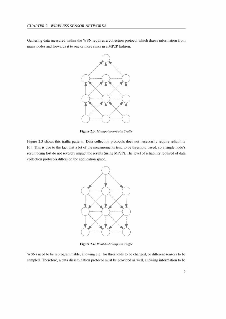
Gathering data measured within the WSN requires a collection protocol which draws information from
many nodes and forwards it to one or more sinks in a MP2P fashion.
Figure 2.3: Multipoint-to-Point Traffic
Figure 2.3 shows this traffic pattern. Data collection protocols does not necessarily require reliability
[6]. This is due to the fact that a lot of the measurements tend to be threshold based, so a single node’s
result being lost do not severely impact the results (using MP2P). The level of reliability required of data
collection protocols differs on the application space.
Figure 2.4: Point-to-Multipoint Traffic
WSNs need to be reprogrammable, allowing e.g. for thresholds to be changed, or different sensors to be
sampled. Therefore, a data dissemination protocol must be provided as well, allowing information to be
5

2.2. TRAFFIC PATTERNS
injected and distributed in the network, starting from one or more sink nodes. This traffic pattern is the
P2MP, and, as shown in Figure 2.4, inverse to the one of data collection. Also, in this case reliability is
a requirement: All nodes in the network need to receive the new data in order to be form a consistent
network.
6
Chapter 3
RADIO TECHNOLOGIES
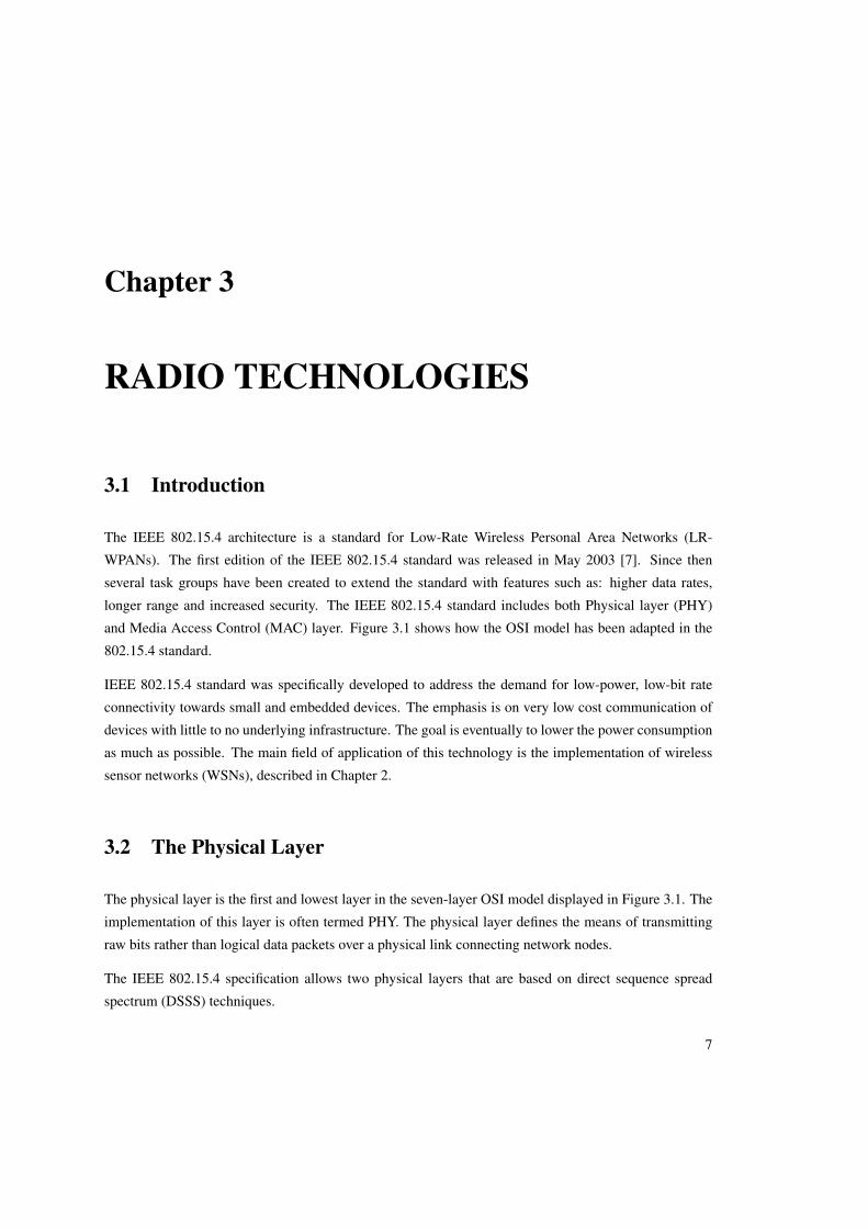
3.1 Introduction
The IEEE 802.15.4 architecture is a standard for Low-Rate Wireless Personal Area Networks (LR-
WPANs). The first edition of the IEEE 802.15.4 standard was released in May 2003 [7]. Since then
several task groups have been created to extend the standard with features such as: higher data rates,
longer range and increased security. The IEEE 802.15.4 standard includes both Physical layer (PHY)
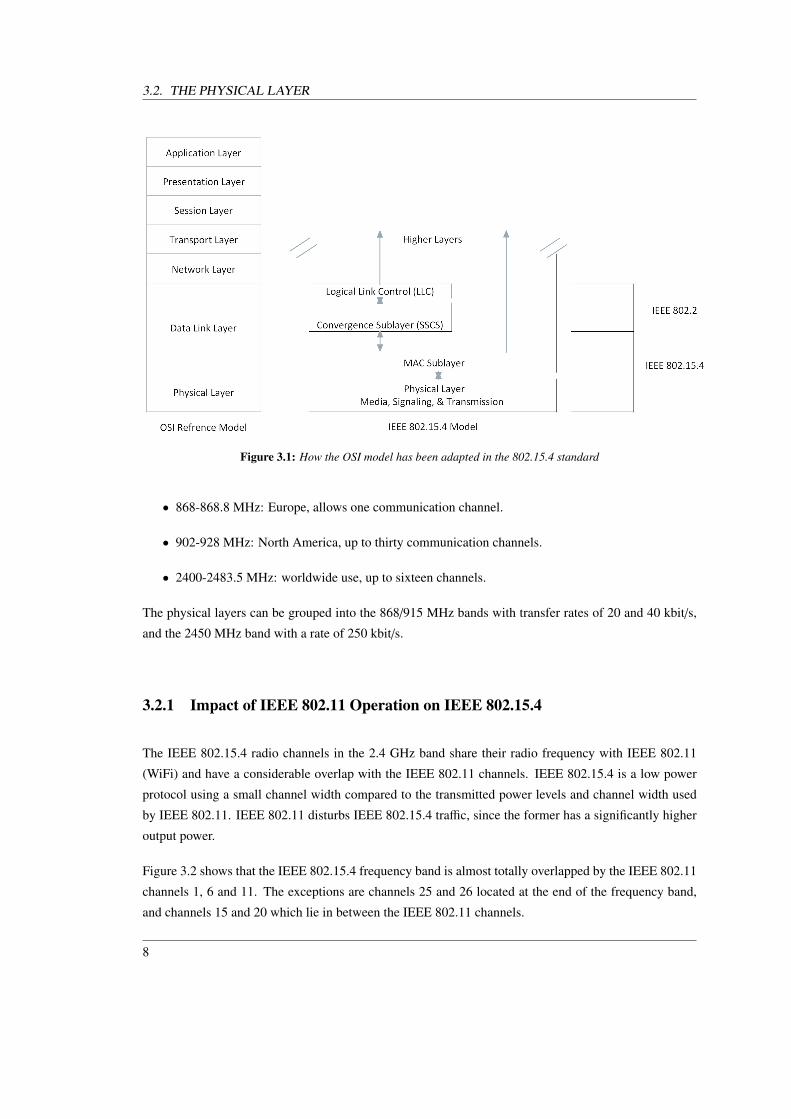
and Media Access Control (MAC) layer. Figure 3.1 shows how the OSI model has been adapted in the
802.15.4 standard.
IEEE 802.15.4 standard was specifically developed to address the demand for low-power, low-bit rate
connectivity towards small and embedded devices. The emphasis is on very low cost communication of
devices with little to no underlying infrastructure. The goal is eventually to lower the power consumption
as much as possible. The main field of application of this technology is the implementation of wireless
sensor networks (WSNs), described in Chapter 2.
3.2 The Physical Layer
The physical layer is the first and lowest layer in the seven-layer OSI model displayed in Figure 3.1. The
implementation of this layer is often termed PHY. The physical layer defines the means of transmitting
raw bits rather than logical data packets over a physical link connecting network nodes.
The IEEE 802.15.4 specification allows two physical layers that are based on direct sequence spread
spectrum (DSSS) techniques.
7
3.2. THE PHYSICAL LAYER
Figure 3.1: How the OSI model has been adapted in the 802.15.4 standard
• 868-868.8 MHz: Europe, allows one communication channel.
• 902-928 MHz: North America, up to thirty communication channels.
• 2400-2483.5 MHz: worldwide use, up to sixteen channels.
The physical layers can be grouped into the 868/915 MHz bands with transfer rates of 20 and 40 kbit/s,
and the 2450 MHz band with a rate of 250 kbit/s.
3.2.1 Impact of IEEE 802.11 Operation on IEEE 802.15.4
The IEEE 802.15.4 radio channels in the 2.4 GHz band share their radio frequency with IEEE 802.11
(WiFi) and have a considerable overlap with the IEEE 802.11 channels. IEEE 802.15.4 is a low power
protocol using a small channel width compared to the transmitted power levels and channel width used
by IEEE 802.11. IEEE 802.11 disturbs IEEE 802.15.4 traffic, since the former has a significantly higher
output power.
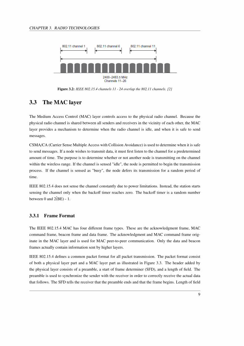
Figure 3.2 shows that the IEEE 802.15.4 frequency band is almost totally overlapped by the IEEE 802.11
channels 1, 6 and 11. The exceptions are channels 25 and 26 located at the end of the frequency band,
and channels 15 and 20 which lie in between the IEEE 802.11 channels.
8
CHAPTER 3. RADIO TECHNOLOGIES
Figure 3.2: IEEE 802.15.4 channels 11 - 24 overlap the 802.11 channels. [2]
3.3 The MAC layer
The Medium Access Control (MAC) layer controls access to the physical radio channel. Because the
physical radio channel is shared between all senders and receivers in the vicinity of each other, the MAC
layer provides a mechanism to determine when the radio channel is idle, and when it is safe to send
messages.
CSMA/CA (Carrier Sense Multiple Access with Collision Avoidance) is used to determine when it is safe
to send messages. If a node wishes to transmit data, it must first listen to the channel for a predetermined
amount of time. The purpose is to determine whether or not another node is transmitting on the channel
within the wireless range. If the channel is sensed "idle", the node is permitted to begin the transmission
process. If the channel is sensed as "busy", the node defers its transmission for a random period of
time.
IEEE 802.15.4 does not sense the channel constantly due to power limitations. Instead, the station starts
sensing the channel only when the backoff timer reaches zero. The backoff timer is a random number
between 0 and 2(̂BE) - 1.
3.3.1 Frame Format
The IEEE 802.15.4 MAC has four different frame types. These are the acknowledgment frame, MAC
command frame, beacon frame and data frame. The acknowledgment and MAC command frame orig-
inate in the MAC layer and is used for MAC peer-to-peer communication. Only the data and beacon
frames actually contain information sent by higher layers.
IEEE 802.15.4 defines a common packet format for all packet transmission. The packet format consist
of both a physical layer part and a MAC layer part as illustrated in Figure 3.3. The header added by
the physical layer consists of a preamble, a start of frame determiner (SFD), and a length of field. The
preamble is used to synchronize the sender with the receiver in order to correctly receive the actual data
that follows. The SFD tells the receiver that the preamble ends and that the frame begins. Length of field
9

3.3. THE MAC LAYER
Figure 3.3: The IEEE 802.15.4 physical layer and MAC layer header formats. [2]
informs the receiver how many bytes will follow.
3.3.2 The Beaconless Mode & Beacon-Enabled Mode
IEEE 802.15.4 supports both beaconless and beacon-enabled operation modes. In the beaconless mode,
the unslotted CSMA/CA protocol is employed to control the channel access among the stations. A station
has to wait for a random backoff period before the start of transmission. If the channel is sensed busy
after a backoff period, the station has to wait another random backoff period before retransmitting.
In the beacon-enabled, the slotted CSMA/CA protocol is employed to control the channel access among
the stations. Prior to random backoff, each station strictly synchronizes its actions and transmissions with
the other stations. The synchronization is done using time slots aligned with beacon slots broadcasted
by the coordinator. After the backoff period, the station starts two consecutive channel sensing, referred
to as the first Clear Channel Assessment (CCA1) and the second CCA (CCA2). The station can only
start transmission if the channel is sensed idle during two consecutive CCA. Otherwise, it has to wait for
another random backoff period [8].
3.3.3 Unslotted CSMA/CA
The MAC layer used in the implementation presented in this thesis supports unslotted CSMA/CA. Unslot-
ted CSMA/CA uses Channel Access Management (CAM) to determine whether or not a node is permitted
to begin a transmission process.
Channel access management is done by using the Clear Channel Assessment (CCA) mechanism, provided
by the physical layer. CCA checks the signal energy on the channel before transmitting. The basic
assumption under CCA is that a packet being transmitted will carry a signal intensity (called a received
signal strength indication or RSSI). If the RSSI exceeds a threshold, it indicates that another node is
currently transmitting, and the MAC layer refrains from sending its own packet. Instead, the MAC layer
waits a specified time and later retries sending the packet.
10

CHAPTER 3. RADIO TECHNOLOGIES
CSMA/CA uses a parameter called number of backoff (NB) which has a initial value of zero. If the CCA
finds the channel busy, a backoff time would be produced and NB would be incremented by 1. NB is set
to certain boundaries (NB max = 4), beyond which the transmission would be aborted to avoid too much
overhead.
CSMA/CA also uses a parameter called the backoff exponent (BE) related to the maximum number of
backoff periods a node will wait before attempting to assess the channel. BE will be initialized to the
value of BE min, which is equal to 3, and cannot assume values larger than BE max, which is equal to
5.
Figure 3.4: IEEE 802.15.4 CSMA/CA algorithm.
Figure 3.4 illustrates the steps of the CSMA/CA algorithm, starting from when the node has data to be
transmitted. First, NB and BE are initialized, and then, the MAC layer will delay any activity for a
random number of backoff periods in the range [0, 2(̂BE)-1] [step (1)]. After this delay, channel sensing
is performed for one unit of time [step (2)]. If the channel is assessed to be busy [step (3)], then the MAC
sub layer will increase both NB and BE by 1, ensuring that BE is not larger than BE max . If the value of
NB is less than or equal to NB max, the CSMA/CA algorithm will return to step (1). If the value of NB
is larger than NB max, the CSMA/CA algorithm will terminate with a "Failure", which means that the
11

3.4. POWER CONSUMPTION
node does not succeed in accessing the channel. If the channel is assessed to be idle [step (4)], the MAC
layer will immediately begin the transmission of data ("Success" in accessing the channel).
3.4 Power Consumption
The power consumption of IEEE 802.15.4 is determined by the current draw of the electrical circuits
that implement the physical communication layer, and by the amount of time during which the radio is
turned on. There are several ways a radio can maintain communication abilities while it is switched off,
described in [2].
Figure 3.5 shows the power consumption of the electrical circuitry of the CC2420 IEEE 802.15.4 transceiver,
as reported by the CC2420 data sheet [2]. It shows that the idle power consumption is significantly lower
than both the listen and the transmit power consumption. In the idle mode, however, the transceiver is
not able to receive any data. The power consumption in the transmit mode is lower than the power con-
sumption in listen mode. The former depends on the output power, which is configurable via software on
a per-packet basis.
Figure 3.5: Power consumption of the CC2420 IEEE 802.15.4 radio transceiver [2].
12

Chapter 4
OMNET++
4.1 Introduction
OMNeT++ is an object-oriented modular discrete event simulator. OMNeT++ and its development en-
vironment is based on Eclipse platform. OMNeT++ itself is not a simulator of anything concrete, but
as described in [3] it provides infrastructure and tools for writing simulations. One of the fundamental
ingredients of this infrastructure is the component architecture for simulation models. Modules can be
reused and combined in various ways like LEGO blocks.
4.2 Modeling Concepts
OMNeT++ modules are often referred to as networks. The top level module is the system module (net-
work module). The system module can contain submodules, which can also contain submodules them-
selves. If modules contain submodules, they are called compound modules. If not, the modules are called
simple modules.
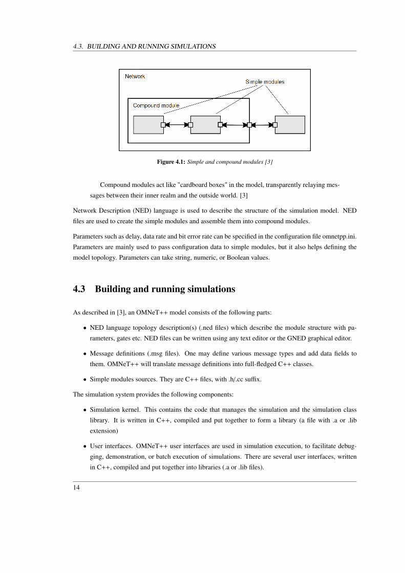
Figure 4.1 illustrates how submodules are grouped into the system modules, and again how sub-submodules
are grouped into submodules. By definition, we can conclude that the system module itself is a compound
module, and that simple modules are at the lowest level of the module hierarchy.
Gates are the input and output interfaces of modules. Modules are linked together by connections between
corresponding gates of two submodules, or a gate of one sub module and a gate of the compound module.
Connections spanning hierarchy levels are not permitted, as they would hinder model reuse.
13
4.3. BUILDING AND RUNNING SIMULATIONS
Figure 4.1: Simple and compound modules [3]
Compound modules act like "cardboard boxes" in the model, transparently relaying mes-
sages between their inner realm and the outside world. [3]
Network Description (NED) language is used to describe the structure of the simulation model. NED
files are used to create the simple modules and assemble them into compound modules.
Parameters such as delay, data rate and bit error rate can be specified in the configuration file omnetpp.ini.
Parameters are mainly used to pass configuration data to simple modules, but it also helps defining the
model topology. Parameters can take string, numeric, or Boolean values.
4.3 Building and running simulations
As described in [3], an OMNeT++ model consists of the following parts:
• NED language topology description(s) (.ned files) which describe the module structure with pa-
rameters, gates etc. NED files can be written using any text editor or the GNED graphical editor.
• Message definitions (.msg files). One may define various message types and add data fields to
them. OMNeT++ will translate message definitions into full-fledged C++ classes.
• Simple modules sources. They are C++ files, with .h/.cc suffix.
The simulation system provides the following components:
• Simulation kernel. This contains the code that manages the simulation and the simulation class
library. It is written in C++, compiled and put together to form a library (a file with .a or .lib
extension)
• User interfaces. OMNeT++ user interfaces are used in simulation execution, to facilitate debug-
ging, demonstration, or batch execution of simulations. There are several user interfaces, written
in C++, compiled and put together into libraries (.a or .lib files).
14

CHAPTER 4. OMNET++
Simulation programs are built from the above components. First, .msg files are translated into C++ code
using the opp_msgc. program. Then all C++ sources are compiled, and linked with the simulation kernel
and a user interface library to form a simulation executable. NED files can either be also translated into
C++ (using nedtool) and linked in, or loaded dynamically in their original text forms when the simulation
program starts.
Figure 4.2: Building and running simulation
When running the program, it starts by reading the configuration file (usually called omnetpp.ini). This
file contains settings that control how the simulation is executed, values for model parameters, etc. The
configuration file can also prescribe several simulation runs; in the simplest case, they will be executed
by the simulation program one after another. An example configuration file is presented in Appendix
B.
15
4.4. SIMPLE MODULES
The output from the simulation is written into files: output vector files, output scalar files , and possibly
the user’s own output files. OMNeT++ provides a GUI tool named Plove to view and plot the contents
of output vector files. The output files are text files, hence it is possible to import desired values into
programs that are independent from OMNeT++. These external programs provide rich functionality for
statistical analysis and visualization [3].
4.4 Simple Modules
This section describes how simple modules communicate. Simple modules are the active modules, written
in C++ using the simulation class library. Here code is written to decide how messages are treated and
forwarded.
4.4.1 Forwarding Messages
Modules communicate by using passing messages. This is typically done by sending messages via gates,
but it is also possible to send them directly to their destination modules. Messages can also be sent within
the sub module. These messages are called self-messages, and can be used to schedule events at a later
time internally in a module. Functions used to send messages between modules are:
int send(cMessage *msg, int gateid);
int sendDelayed(cMessage *msg, simtime_t delay, int gateid);
• msg is the message the module is to send.
• delay is the amount of time the message should wait before it is to be sent.
• gateid is the ID of the gate the message is sent from.
Modules uses the send() and sendDelayed() functions which it inherits from cSimpleModule to send
messages between modules. To send a unicast message, a destination network address needs to be set. If
a message is sent without a specified destination L3 address, a broadcast address is used instead.
Modules can also send "messages" internally using self-messages to schedule events. An event can for
instance be the scheduling of a message at a future point in time.
int scheduleAt(simtime_t t, cMessage *msg);
cMessage *cancelEvent(cMessage *msg);
• simtime_t t is the time when the message should be sent.
• msg is the message the module is to send.
16
CHAPTER 4. OMNET++
The simulation time returns the exact time of the simulation duration in seconds. If the purpose is to
schedule an event later in the simulation, the desired delay must be added to the simulation time.
When the time of the scheduled event has elapsed, the message will be delivered back to the module
via receive() or handleMessage() at simulation time t. This function can be used to implement timers or
timeouts. To remove a given message from the future events, the cancelEvent() function can be used.
The message needs to have been sent using the scheduleAt() function for it to have an effect, and can be
used to cancel a timer implemented with scheduleAt(). If the message is not currently scheduled, nothing
happens.
4.4.2 Treating Messages
Data members such as values of module parameters, gate indices, routing information, etc, can be ini-
tialized by the initialize() function. The initialize function also schedule initial event(s) which trigger the
first call(s) to handleMessage(). After the first call, handleMessage() must take care to schedule further
events for itself so that the "chain" is not broken. Scheduling events is not necessary if your module only
has to react to messages coming from other modules.
The handleMessage() function will be called for every message that arrives at the module. The func-
tion does nothing by default, but the user can redefine it in subclasses and add the message processing
code. No simulation time elapses within a call to handleMessage(). Modules with handleMessage() are
not started automatically. The user have to schedule self-messages for the initialize() function to start
handleMessage() function without receiving a message from other modules.
OMNeT++ specifies a finish() function normally used to record statistics information accumulated in
data members of the class at the end of the simulation.
17

4.5. MIXIM FRAMEWORK
4.5 MiXiM Framework
MiXiM provides a framework that supports simulations of a fixed wireless sensor network. It offers
detailed modules of radio wave propagation interference estimation, radio transceiver power consumption
and wireless MAC protocols. The framework also provides basic modules that can be derived in order to
implement own modules.
MiXiM provides several applications which can be used but they are not documented and the source
codes have to be studied to understand them. The models in OMNeT++ are compound from several C++
objects and wired together using NED. The modules have hierarchical structure and the communication
between them is performed using messages.
4.5.1 Node Structure
There are currently no well-known routing protocols officially released for MiXiM. There are groups that
might have implemented several protocols (such as with all the open-source simulators). The developer is
either referred to finding some useful source codes from another sources or to implement desired routing
protocol on his own (starting with MiXiMs BaseNetworkLayer). However, there are several routing
paradigms that can be used within MiXiM (e.g.source-to-sink, any-to-any, local neighbourhood) [?]. The
routes are specified in a configuration file.
Figure 4.3: BaseNetwork node structure.
4.5.2 Support for Signal Propagation Modelling
The signal is delivered using connectionManager and can be attenuated by one or more wireless channel
models (called Analogue Models) specified in config.xml configuration file. SimplePathlossModel rep-
resents the free space model according to Friis formula. LogNormalShadowing can be used to calculate
deviations (mean, standard deviation and interval of attenuation changes are parameterized). The thermal
noise (default -110 dBm) can also be configured.
18
CHAPTER 4. OMNET++
The packet reception decision is itself practically influenced by the so-called Decider. One, or more
Decider can be defined in config.xml. DeciderResult802154Narrow and SNRThresholdDecider are the
most interesting for our requirements. The former represents an approach of IEEE 802.15.4 commu-
nications but it has not been fully implemented yet. BER is calculated only for MSK (Minimum Shift
Keying) modulation technique. The latter works in such a way that the signal is first checked whether it
is above the sensitivity of the node and then if it is above SNR threshold, which can be parameterized in
config.xml.
19
Chapter 5
ROUTING IN WSNs
5.1 Introduction
Routing is a process of selecting paths in a network along which to send network traffic. Once the paths
have been selected, data traffic is forwarded from one endpoint of the transmission via intermediate nodes
to the other endpoint. Routing algorithms are used to determine the "best" paths towards the destination
according to one or more metrics, depending on the application requirements.
For example, one widely used metric selects the route with the least amount of hops trough intermediate
nodes towards the destination. Alternative metrics could be to use the best link quality, or least energy
consumption. More on routing metrics for WSNs can be found in [9].
The restrictions imposed by WSNs, which were presented in Chapter 2, add further requirements to
suitable routing algorithms. The algorithms have to efficiently deal with an ever changing topology,
whilst imposing as little control traffic overhead as necessary on the network, as the transmission of
messages is very costly in terms of energy [10].
The routing protocol needs to compute routes between nodes in the network in order to actually be able
to send data to each node. Proactive protocols periodically re-compute these routes, whereas reactive
protocols do so only on demand, i.e. when a data packet need to be transmitted. The following section
describes the difference between proactive and reactive protocols and give examples of routing protocols
for each category.
20
CHAPTER 5. ROUTING IN WSNS
5.1.1 Reactive Protocols
In reactive routing protocols, no path to the destination is currently known when a packet needs to be
forwarded. Routes are acquired by nodes on demand by triggering a route discovery process, e.g. by
diffusing a route request packet through the network and then wait for a response for the destination node.
This response might take time to arrive, causing the packet delivery to be delayed. The overhead of control
packets in a reactive protocol is depending on the amount of data traffic in the network. Reactive protocols
do not require each node to store routes for the entire network, rather computed only for destinations to
which data traffic is to be forwarded. The Ad-hoc On-Demand Distance Vector (AODV) [11] is an
example of a reactive protocol.
5.1.2 Proactive Protocols
In proactive routing protocols, nodes regularly compute routing tables of the complete network, thus
pre-provisioning all possible paths for the entire network topology. Hence, there is no delay imposed
by route acquisition before sending the data traffic to its destination. However, a certain amount of
control traffic is needed to maintenance the routing tables, and keep them consistent over the whole
network. The Optimized Link State Routing protocol (OLSR) [12] is a prominent example of a proactive
protocol.
5.2 Flooding Algorithm
A variety of routing protocols exist for WSNs [13], which uses different strategies to address the restric-
tions introduced in WSNs. The most straightforward way to diffuse information in a WSN is to use a
flooding algorithm. The flooding algorithm transmits broadcast data which are consecutively retrans-
mitted in order to make them arrive at the intended destination. To prevent broadcast storms, several
mechanisms are available: nodes check for duplicates, i.e. messages they already received, and packets
may contain information about how many times they are allowed to be retransmitted.
The drawbacks of the flooding algorithm is that nodes redundantly receive multiple copies of the same
data messages. Inconveniences are highlighted when the number of nodes in the network increases.
21
5.3. RPL ROUTING PROTOCOL
5.3 RPL ROUTING PROTOCOL
The Internet Engineering Task Force (IETF) has a Routing Over Low power and Lossy networks (ROLL)
working group currently specifying an IPv6-based unicast routing protocol for WSNs, denoted RPL
("IPv6 Routing Protocol for Low power and Lossy Networks"[5]). IETF ROLL working group have
extensively evaluated existing routing protocols such as OSPF, AODV, IS-IS and OLSR and concluded
that they are not suitable for the routing requirements specified in [14], [15], [16] and [17].
RPL is a proactive routing protocol, constructing its routes in periodic intervals. RPL may run one or
more RPL instances. Each of the instances has its own topology built with its own unique appropriate
metric. Nodes can join multiple RPL instances but only belong to one DODAG within each instance.
Starting from one of more root nodes, each Instance builds up a tree-like routing structure in the network,
resulting in a Destination-Oriented Directed Acyclic Graph (DODAG). For the rest of this chapter, the
protocol is explained for one RPL Instance with one DODAG.
5.3.1 Topology Formation
Topology formation in RPL starts with designating one node as root node. The configuration parame-
ters of the network are determined by the root node, and disseminated to the network using a DODAG
Information Object (DIO) message. For the content of the DIO message and its transmission rules in
more detail, see Section 5.3.3.1. The mandatory information contained in a DIO comprises amongst
others:
• RPLInstanceID for which the DIO is sent,
• the DODAGID of the RPLInstance of which the sending node is part of,
• the current DODAG version number, and
• the node’s rank within the DODAG
The RPLInstanceID is a unique identifier of an RPL Instance in a network. The DODAGID serves the
same purpose: to uniquely identify a DODAG in an RPL Instance.
The rank represents the nodes individual position relative to the root node. The rank increases in the down-
ward direction from the root towards the leaf nodes. The node’s rank gets calculated by a Object Function
(OF) which uses a metric to determine the node’s desirability (in terms of application goals, which might,
e.g., be load balance for energy preservation) as a next hop on a route to the root node.
When forming the DODAG, each node is required to select a parent from its neighbors. Accordingly, the
node has to calculate its own rank so that it is larger than any of its parents. In this way, the formation of
loops in the routing structure is prevented.
22
CHAPTER 5. ROUTING IN WSNS
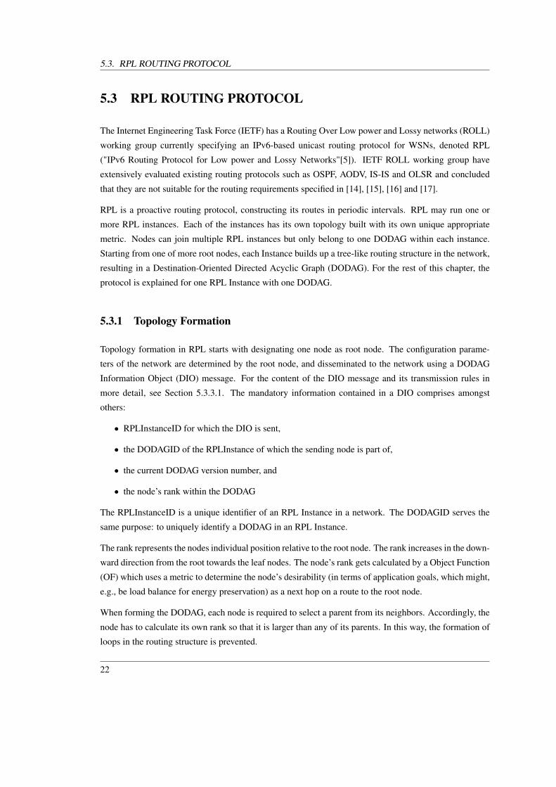
Figure 5.1: Example Network: circles illustrates wireless sensor nodes, connected with 802.15.4 links depicted bydashed lines.
The OF can be used to tailor RPL closely to serve a specific application. To give an example, a node’s
energy level or its power resource could be used in he OF to calculate the rank. When a node then
selects a parent, it will choose the neighbor with the lowest rank, hence the preferable node energy or
power resource. For the sake of simplicity, the hop count metric is used as the OF in the following
example.
The root node starts the DODAG formation by broadcasting a DIO message to its neighbor as illustrated
in Figure 5.2 (round 1). The root node of a DODAG is the only node allowed to initiate the diffusion of
DIOs. Throughout the whole topology formation, RPLInstanceID and the DODAGID remain unchanged.
The only field updated whilst the DIO message are traversing the network, is the rank.
The root node has a rank equal to 0, since the distance from itself is zero. When the neighbors receive
the broadcast DIO message, they calculate their rank according to the OF by computing its hop count
distance to the root node and sets its rank to 1.
From the DIO message received, each node retains a candidate neighbor set, in which it keeps track of the
neighbors with lower or equal rank then itself. The candidate neighbor set is used to select parent nodes,
which have to have a lower rank than itself. If there are more than one selected parent, the node elects
a so-called preferred parent, which serves as the node’s next hop when routing a data packet towards
the root. This choice is determined by the OF. In round 1, there is only one candidate parent, so they
pick the root as their preferred parent. In Figure 5.3, this relationship is represented by the bold plain
arrows.
23
5.3. RPL ROUTING PROTOCOL
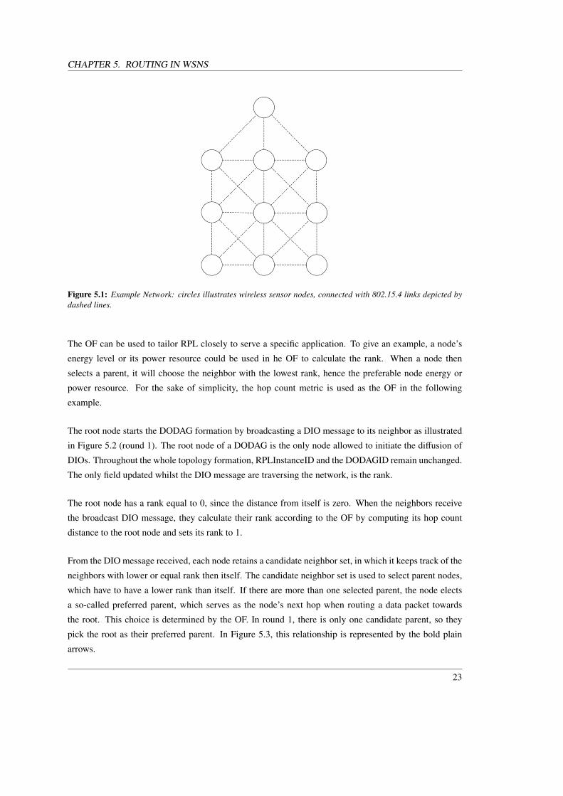
After calculating its rank, each node broadcast the updated DIO message to its neighbors (Figure 5.2,
round 2). The root node will discard the DIO messages received since they originates from nodes with
higher rank than itself. The other neighbors will repeat the process of calculating its own rank according
to the OF, and update the DIO message before broadcasting it to their neighbors.
In Figure 5.2, there are several nodes in the node’s parent set that might fulfill the conditions imposed by
the OF, making them qualified as preferred parent. In this case, as described later (in Section 6.4.1.4), the
preferred parent will be selected on the basis of a set of rules.
Figure 5.2 (round 3) displays the last step of the topology formation: all nodes of the network have
received DIO messages and joined the DODAG by calculating their rank, whilst the nodes have selected
proffered parents represented by the bold plain arrows in Figure 5.3.
Figure 5.2: DIO messages broadcasted (indicated by arrows) to their neighbors towards leaf nodes. The numbersindicate the node’s respective rank, i.e., their logical distance to the root.
5.3.2 Traffic Flows Supported by RPL
By default, RPL provides a mechanism for multipoint-to-point (MP2P) data traffic from nods within the
network to the root node. This traffic flow is called "upward" and is enabled by the DIO mechanism,
described in Section 5.3.3.1.
RPL also provides a mechanism to support "downward" traffic flow, which is needed to enable point-
to-multipoint (P2MP) or point-to-point (P2P) traffic patterns. Downward routes are established using
Destination Advertisement Object (DAO) messages. P2P traffic is routed "upwards" until it reaches a
common ancestor which knows a route "down" the DODAG to its destination. The specification distin-
guishes between storing and non-storing traffic mode. In storing mode, all nodes keep state of routes to
24

CHAPTER 5. ROUTING IN WSNS
Figure 5.3: The parents are selected (indicated by the bold plain arrows) before the DIO message are updated andrebroadcasted illustrated in Figure 5.2. This Figure shows all parents selected when the DIO message has propagatedto the leaf nodes. The rules deciding the selection of parents are described in Chapter 5.
other nodes. In non-storing mode, intermediate nodes do not know any downward routes, so packets are
always routed to the root node of its DODAG and then source-routed to its destination.
In respect to Figure 5.3, the direction from the leaf nodes towards the DAG roots is referred to as the "up"
direction. Hence, the direction from the DAG roots towards the leaf nodes are referred to as the down
direction. A node’s rank defines the node’s individual position in the DODAG, relative to other nodes
with respect to the DODAG root. Rank strictly increases in the "down" direction and strictly decreases in
the "up" direction. How the rank is calculated depends on the DAG’s Objective Function (OF). Witch OF
the DODAG uses are identified by the Objective Code Point (OCP). The rank is also used when selecting
a parent, where traffic is sent on the path towards the DODAG root (which has the lowest rank in the
DODAG).
25
5.3. RPL ROUTING PROTOCOL
5.3.3 RPL Control Messages
This section will describe the three different messages used by RPL: DIO, DAO and DIS messages, and
fields included. Transmission scheduling rules for the different RPL messages are also presented.
5.3.3.1 DODAG Information Object (DIO)
0 1 2 3
0 1 2 3 4 5 6 7 8 9 0 1 2 3 4 5 6 7 8 9 0 1 2 3 4 5 6 7 8 9 0 1
+-+-+-+-+-+-+-+-+-+-+-+-+-+-+-+-+-+-+-+-+-+-+-+-+-+-+-+-+-+-+-+-+
| RPLInstanceID |Version Number | Rank |
+-+-+-+-+-+-+-+-+-+-+-+-+-+-+-+-+-+-+-+-+-+-+-+-+-+-+-+-+-+-+-+-+
|G|0| MOP | Prf | DTSN | Flags | Reserved |
+-+-+-+-+-+-+-+-+-+-+-+-+-+-+-+-+-+-+-+-+-+-+-+-+-+-+-+-+-+-+-+-+
| |
+ +
| |
+ DODAGID +
| |
+ +
| |
+-+-+-+-+-+-+-+-+-+-+-+-+-+-+-+-+-+-+-+-+-+-+-+-+-+-+-+-+-+-+-+-+
| Option(s)...
+-+-+-+-+-+-+-+-+
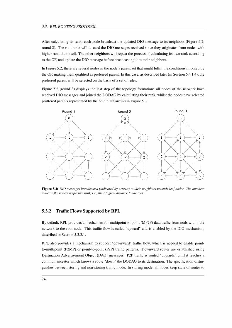
Figure 5.4: The DIO Base Object [1]
Figure 5.4 shows the DIO message format. The DIO message format consist of nine different fields of
witch four was necessary for the measurements preformed in this paper’s implementation. The fields that
are excluded are the once required when there is multiple DODAGS. The implementation consist of a
single DODAG with a single RPL instance.
• Mode of Operation (MOP) - The Mode of Operation (MOP) is always set to storing mode.
• Rank - 16-bit unsigned integer indicating the DODAG rank of the node sending the DIO message.
• Destination Advertisement Trigger Sequence Number (DTSN): 8-bit unsigned integer set by the
node issuing the DIO message. The Destination Advertisement Trigger Sequence Number (DTSN)
flag is used as part of the procedure to maintain downward routes. The details of this process are
described in Section 5.3.3.2.5.
• Flags: 8-bit unused field reserved for flags. The field MUST be initialized to zero by the sender
and MUST be ignored by the receiver.
5.3.3.1.1 DIO Base Rules .
26

CHAPTER 5. ROUTING IN WSNS
The process of creating a DODAG starts when the DODAG root sends out DAG Information Option
(DIO) messages using link-local multicasting. When a DIO message is received, the receiving node must
first determine whether or not the DIO message should be accepted for further processing. Presented
below are the criteria’s for further processing of a DIO message as standardized in [1].
1. If the DIO message is malformed, then the DIO message is not eligible for further processing and
a node MUST silently discard it.
2. If the sender of the DIO message is a member of the candidate neighbor set and the DIO message
is not malformed, the node MUST process the DIO.
The DIO message contains a 16-bit unsigned integer indicating its respective rank in the DODAG (i.e.
its distance from the root according to some metric(s), in the simplest form hop count). See Section ??.
Upon receiving a (number of such) DIO messages a node will calculate its own rank such that it is greater
than the rank of each of its parents, and will itself start emitting DIO messages. Neighbor(s) with the
lowest rank are selected as parent(s). DIO messages received from nodes which has a higher rank then
the parent selected are discarded. Thus, the DODAG formation starts at the root, and spreads gradually
until it reaches leaf nodes.
RPL contains rules, restricting the ability for a router to change its rank. Specially, a router is allowed to
assume a smaller rank than previously advertised (i.e. to logically move closer to the root) if it discovers a
parent advertising a lower rank (and it must then disregard all previous parents with higher ranks), while
the ability for a router to assume a greater rank (i.e. to logically move farther from the root) in case all its
former parents disappear, is restricted to avoid count-to-infinity problems. The root can trigger "global
recalculation" of the DODAG by way of increasing a sequence number in the DIO messages.
5.3.3.1.2 The Trickle Algorithm .
DIO transmission is governed uses a trickle timer to periodically emit control messages. The trickle
timers use dynamic timers that govern the sending of DIO messages in an attempt to reduce redundant
messages. The interval between sending control messages are increased exponentially until it reaches a
constant rate also called the maximum interval (I_max). In other words; when the DODAG stabilizes,
DIO messages gets sent less frequent. If inconsistencies are detected, the interval resets to its minimum
value. This allows fast generation of DIO messages when there is a need to propagate new information
down the DAG. Below a list of inconsistencies causing the interval being reset is presented.
• The node joins a new DODAG
• The node moves within a DODAG
• The node receives a modified DIO message from a DODAG parent
27
5.3. RPL ROUTING PROTOCOL
• A DODAG parent forwards a packet intended to move up, indicating an inconsistency and possible
loop
• A metric communicated in the DIO message is determined to be inconsistent, as according to a
implementation specific path metric selection engine
• The rank of a DODAG parent has changed.
The trickle timer has to have three parameters configured: the minimum interval size I_min, the maximum
interval size I_max or the number of times the interval is doubled I_doubling and a redundancy constant
k. If you know I_min and I_max you can calculate the number of doublings of the minimum interval size
by taking (base-2 log (max/min)). The redundancy constant, k, is a natural number (an integer greater
than zero).
For RPL simulations I_min is set to 1 second and I_doubling is equal to 16. This gives a maximum
interval equal to 18.2 hours, between two control packets under a steady network condition. In addition
to these three parameters, Trickle maintains three variables:
• I, the current interval size.
• t, a time within the current interval.
• c, a counter.
Presented below are the six rules of the trickle algorithm as described in RFC-6206 [18].
1. When the algorithm starts execution, it sets I to a value in the range of [Imin, Imax] – that is, greater
than or equal to Imin and less than or equal to Imax. The algorithm then begins the first interval.
2. When an interval begins, Trickle resets c to 0 and sets t to a random point in the interval, taken
from the range [I/2, I), that is, values greater than or equal to I/2 and less than I. The interval ends
at I.
3. Whenever Trickle hears a transmission that is "consistent", it increments the counter c.
4. At time t, Trickle transmits if and only if the counter c is less than the redundancy constant k.
5. When the interval I expires, Trickle doubles the interval length. If this new interval length would
be longer than the time specified by Imax, Trickle sets the interval length I to be the time specified
by Imax.
6. If Trickle hears a transmission that is "inconsistent" and I is greater than Imin, it resets the Trickle
timer. To reset the timer, Trickle sets I to Imin and starts a new interval as in step 2. If I is equal
to Imin when Trickle hears an "inconsistent" transmission, Trickle does nothing. Trickle can also
reset its timer in response to external "events".
28

CHAPTER 5. ROUTING IN WSNS
5.3.3.2 Destination Advertisement Object (DAO)
When establishing downward routes, DAO messages are used to propagate destination information up-
wards along the DODAG. In storing mode the DAO-messages are unicast by the child to the selected
parent(s). In non-storing mode the DAO message is unicasted to the DODAG root. A Destination Ad-
vertisement Acknowledgement (DAO-ACK) message may be used. The DAO-ACK is sent as a uni-
cast packet by DAO recipient (a DAO parent or DODAG root) in response to a unicast DAO message
[1].
5.3.3.2.1 Format of the DAO Base Object .
0 1 2 3
0 1 2 3 4 5 6 7 8 9 0 1 2 3 4 5 6 7 8 9 0 1 2 3 4 5 6 7 8 9 0 1
+-+-+-+-+-+-+-+-+-+-+-+-+-+-+-+-+-+-+-+-+-+-+-+-+-+-+-+-+-+-+-+-+
| RPLInstanceID |K|D| Flags | Reserved | DAOSequence |
+-+-+-+-+-+-+-+-+-+-+-+-+-+-+-+-+-+-+-+-+-+-+-+-+-+-+-+-+-+-+-+-+
| |
+ +
| |
+ DODAGID* +
| |
+ +
| |
+-+-+-+-+-+-+-+-+-+-+-+-+-+-+-+-+-+-+-+-+-+-+-+-+-+-+-+-+-+-+-+-+
| Option(s)...
+-+-+-+-+-+-+-+-+
Figure 5.5: The DAO Base Object [1]
Figure 5.5 shows the DAO message format. The DAO message format consist of seven different fields
of witch four were essential for measurements done in this thesis. The functionalities implemented are
presented below as they are in [1]
• The ’K’ flag indicates that the recipient is expected to send a DAO-ACK back.
• Flags: The 6-bits remaining unused in the Flags field are reserved for flags. The field MUST be
initialized to zero by the sender
• DAOSequence: Incremented at each unique DAO message from a node and echoed in the DAO-
ACK message.
5.3.3.2.2 Storing Mode .
The Mode of Operation (MOP) used by the implementation presented in this paper, is storing mode. In
storing mode operation, a node MUST NOT address unicast DAO messages to nodes that are not DAO
29
5.3. RPL ROUTING PROTOCOL
parents. DAOs advertise what destination addresses and prefixes a node has routes to. All non-root, non-
leaf nodes MUST store routing table entries for destinations learned from DAOs. When a node receives
a packet with a destination address, the next hop is always decided by examining its routing table.
If a node receives a DAO message containing newer information that outdates the information already
stored at the node, the node must generate a new DAO message and transmit it. The new DAO generated
should be unicasted to each of its parents. If a node decides to remove one of its DAO parents, it should
send a No-Path DAO message to that removed DAO parent, to invalidate the existing route.
5.3.3.2.3 DAO Base Rules .
DAO Base Rules applied in this thesis implementation are listed below as described in and selected from
[1].
1. If a node sends a DAO message with newer or different information than the prior DAO message
transmission, it MUST increment the DAOSequence field by at least one. A DAO message trans-
mission that is identical to the prior DAO message transmission MAY increment the DAOSequence
field.
2. A node MAY set the ’K’ flag in a unicast DAO message to solicit a unicast DAO-ACK in response
in order to confirm the attempt.
3. A node receiving a unicast DAO message with the ’K’ flag set SHOULD respond with a DAO-
ACK. A node receiving a DAO message without the ’K’ flag set MAY respond with a DAO-ACK,
especially to report an error condition.
4. A node that sets the ’K’ flag in a unicast DAO message but does not receive a DAO-ACK in response
MAY reschedule the DAO message transmission for another attempt, up until an implementation-
specific number of retries.
5. Nodes SHOULD ignore DAOs without newer sequence numbers and MUST NOT process them
further.
5.3.3.2.4 DAO Transmission Scheduling .
Listed below are the criteria for transmitting a DAO message in a DODAG as specified in [1]:
1. On receiving a unicast DAO message with updated information, such as containing a Transit Infor-
mation option with a new Path Sequence, a node SHOULD send a DAO. It SHOULD NOT send
this DAO message immediately. It SHOULD delay sending the DAO message in order to aggregate
DAO information from other nodes for which it is a DAO parent.
30

CHAPTER 5. ROUTING IN WSNS
2. A node SHOULD delay sending a DAO message with a timer (DelayDAO). Receiving a DAO
message starts the DelayDAO timer. DAO messages received while the DelayDAO timer is active
do not reset the timer. When the DelayDAO timer expires, the node sends a DAO.
3. When a node adds a node to its DAO parent set, it SHOULD schedule a DAO message transmission.
DelayDAO’s value and calculation is implementation-dependent. DEFAULT_DAO_DELAY is set to 1
second. Selecting a proper DAODelay, giving the node time to aggregate DAO information from other
nodes for which it is a DAO parent can greatly reduce the number of DAOs transmitted.
5.3.3.2.5 Triggering DAO Messages .
DAO messages are triggered using a DAO Trigger Sequence Number (DTSN). This number is maintained
in each node, and are communicated through DIO messages. If a node hears one of its parents increment
its DTSN, the node MUST schedule a DAO message transmission using rules in section 5.3.3.2.3 and
section 5.3.3.2.4.
DTSN MAY be incremented in a storing mode of operation, as part of routine routing table update and
maintenance. The incremented DTSN will trigger a set of DAO updates from its immediate children, and
the DAO information will propagate hop-by-hop up the DODAG. This makes it unnecessary to trigger
DAO updates from entire the sub-DODAG.
In the general, a node may trigger DAO updates according to implementation specific logic, such as
based on the detection of a downward route inconsistency or occasionally based upon an internal timer
[1].
31
5.3. RPL ROUTING PROTOCOL
5.3.3.3 DODAG Information Solicitation (DIS)
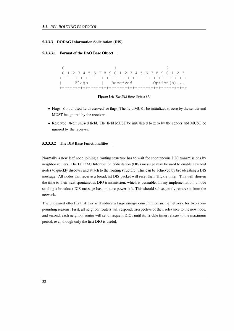
5.3.3.3.1 Format of the DAO Base Object .
0 1 2
0 1 2 3 4 5 6 7 8 9 0 1 2 3 4 5 6 7 8 9 0 1 2 3
+-+-+-+-+-+-+-+-+-+-+-+-+-+-+-+-+-+-+-+-+-+-+-+-+
| Flags | Reserved | Option(s)...
+-+-+-+-+-+-+-+-+-+-+-+-+-+-+-+-+-+-+-+-+-+-+-+-+
Figure 5.6: The DIS Base Object [1]
• Flags: 8 bit unused field reserved for flags. The field MUST be initialized to zero by the sender and
MUST be ignored by the receiver.
• Reserved: 8-bit unused field. The field MUST be initialized to zero by the sender and MUST be
ignored by the receiver.
5.3.3.3.2 The DIS Base Functionalities .
Normally a new leaf node joining a routing structure has to wait for spontaneous DIO transmissions by
neighbor routers. The DODAG Information Solicitation (DIS) message may be used to enable new leaf
nodes to quickly discover and attach to the routing structure. This can be achieved by broadcasting a DIS
message. All nodes that receive a broadcast DIS packet will reset their Trickle timer. This will shorten
the time to their next spontaneous DIO transmission, which is desirable. In my implementation, a node
sending a broadcast DIS message has no more power left. This should subsequently remove it from the
network.
The undesired effect is that this will induce a large energy consumption in the network for two com-
pounding reasons: First, all neighbor routers will respond, irrespective of their relevance to the new node,
and second, each neighbor router will send frequent DIOs until its Trickle timer relaxes to the maximum
period, even though only the first DIO is useful.
32

Chapter 6
THE RPL IMPLEMENTATION FOROMNET++
This chapter presents the implementation of RPL for OMNeT++ and the different approaches that were
taken when implementing the core functionality of RPL. For implementation code, see Appendix A.
6.1 Introduction
In 2008 the Internet Engineering Task Force (IETF) formed a new working group called ROLL. Its objec-
tive was to specify routing solutions for low power and lossy networks. The working group is currently
designing a new routing protocol called RPL (Routing Protocol for Low Power and Lossy Networks)
which is a work in progress towards a RFC in IETF in [1]. The RPL specification is well structured, but
is still under development.
The RPL specification classifies functionality into three classes; functionality that MUST be imple-
mented, functionality that SHOULD be implemented and functionality that MAY be implemented. Func-
tionality that MUST be implemented is critical for the basic functionality of the protocol, and cannot be
omitted. Functionality that SHOULD be implemented is necessary for the protocol to function, but can
be skipped, although this is not recommended. Functionality that MAY be implemented is often extra
functionality and optimizations of already specified functionality.
The implementation presented in this thesis follows the functionalities that MUST be implemented, and
selects relevant functionalities from SHOULDs and MAYs depending on their influence on the perfor-
mance evaluation. Functionalities described in [1] which does not have any effect on the measurements
to be done are NOT implemented. For instance, the protocol is implemented for one RPL Instance with
33

6.1. INTRODUCTION
one DODAG, which excludes a number of functionalities. Chapter 5 explains why the choice was taken
to look at a single RPL instance within a single DODAG.
Functionalities required in the implementation which were not described in [1] was: The handling a dead
node described in section 6.4.1.3, and the transmission of the initial DAO message described in Section
6.3.1.2
This thesis contribution is to provide a performance evaluation of RPL while using two metrics of interest;
hop count object and node energy object. The metrics uses different approaches to determine the best
possible route towards destination. Hop count selects routes using number of hops to destination, while
the node energy object selects its route depending on the intermediate nodes residual capacity. The node
energy object will certainly distribute data traffic between nodes in a more sophisticated manner, but at
what cost?
The protocol behaviors is reproduced using theoretical values and topologies of wireless sensor networks
developed in a discrete event simulator. MiXiM [?], provides a framework created for mobile and fixed
wireless networks.
6.1.1 The Tools used
6.1.1.1 Integrated Development Environment (IDE)
An Integrated Development Environment (IDE) is a programming environment which can provide fea-
tures such as code editing, compilation, debugging and a graphical user interface (GUI) builder. The
implementation was developed using the OMNeT++ IDE. Eclipse IDE [?] where used to filter .sca
output data into .txt files readable for Gnuplot, in addition to create network structures used in simu-
lations.
6.1.1.2 Gnuplot
Gnuplot is a command-line drive graphing utility. In the simulation, Gnuplot has been used to draw
graphs of data retrieved from both filtered OMNeT++ data. It was preferred due to its simplicity, and
ability to directly generate Encapsulated PostScript (graphical file format, .eps) which is convenient if
writing in LATEX. Scripts were slightly modified (colors and output) versions of scripts found on The
Linux Foundation web site [19]. For all other, discerent scripts were written for each graph. There are
too many to include in this paper, but a selected script can be found in Appendix D.
34
CHAPTER 6. THE RPL IMPLEMENTATION FOR OMNET++
6.1.1.3 Visual Paradigm
A powerful, cross-platform and feature-rich UML tool that supports the latest UML standards. Visual
Paradigm for UML Community Edition (VP-UML CE) provides the most easy-to-use and intuitive visual
modeling environment with rich set of export and import capabilities such as XMI, XML, PDF, JPG, EPS
and more[20].
6.1.1.4 The Figures Used
In the figures classes are represented using a pseudo UML notation. The fields and methods in the classes
are given as they would have been in the source code, although abbreviated. The thin arrows represent
method calls.
In the handle[X]Message methods, flow diagrams are used to illustrate how messages are processed. The
triangles represents a decision in form of a Boolean or an if statement. the rectangular forms represent
function calls.
35

6.2. OMNET++ NETWORK STRUCTURE
6.2 OMNeT++ Network Structure
As described in Chapter 4, modules containing submodules are called compound modules, while modules
which does not contain submodules are called simple modules.
The Wireless Sensor Network (WSN) is a compound module, containing an arbitrary number of sub
modules (in this implementation, wireless sensor nodes) displayed in Figure 6.1b. Inside each of these
wireless sensor nodes, there are a number of simple modules and one compound module containing the
two simple modules displayed in Figure 6.1c. The simple modules are the active modules, written in C++
using the simulation class library. Every node in the network contains the exact same structure of simple
modules.
(a) BaseNetwork (b) BaseNode (c) BaseNic
Figure 6.1: Compound of modules.
It is natural to first examine simple modules which communicates with each other by passing messages
through gates, see Chapter 4 for detailed information on OMNeT++.
An application module is a higher layer module included in the MiXiM framework. The application
module was heavily modified to fulfill the purposes of this implementation. The main purpose of the
application module is to send traffic to provoke behavior desirable for measurements to be made.
The RPL and Routing module are the modules imposing the RPL functionalities on the existing MiXiM
framework modules. Creating and connecting a new module such as RPL to the existing infrastructure of
MiXiM requires a Network Description (NED) file, see Chapter 4. The NED file assembles the simple
modules into a compound module, as displayed in Figure 6.1b.
36

CHAPTER 6. THE RPL IMPLEMENTATION FOR OMNET++
Figure 6.2: Example network used in Chapter 5, presented in OMNeT++.
The RPL module defines gates and parameters in a NED file, enabling it to connect and communicate
with other simple module within a compound module. The simple modules are written in C++ and
implements functionalities on how to transmit and handle received messages. The RPL simple module
was implemented as described in the protocol specifications of RPL [1].
A Routing module was created to provide the possibilities for P2MP and MP2P traffic described in Chap-
ter 2. By using a storing mode of operation, each node maintains a routing table containing routes to
nodes lower than itself in the hierarchical structure. Each node also contains a default gateway which is
the route to it preferred parent.
RPL is implemented as a higher layer protocol sending messages down through the network layer towards
the Network Interface Card (NIC), and finally out on the air. The network layer is responsible for packet
forwarding, and uses the routing module to route messages through intermediate nodes. If the message
received is a unicast message with a specified L3 network address, it will pass through the Routing module
before getting transmitted to the NIC. Whereas if the message does not contain a specified L3 network
address, it is handled as a broadcast message and sent directly to the NIC.
The NIC is a compound module containing two simple modules; a MAC layer and a PHY layer. The
functionalities of the radio where presented in Chapter 3, and are not further discussed. When the radio
channel is available, the airframe message is sent either by broadcast or unicast, since multicast is not
supported in this implementation. The wireless sensor nodes are placed within the playground of the
network compound module.
The nodes within the playground are "connected" if they lie in the range of each other’s transmission
37
6.2. OMNET++ NETWORK STRUCTURE
range (i.e. the coverage area of the wireless sensor node, controlled by the Mobility module). If nodes
are connected, it is displayed by an arrow, shown in Figure 6.2. The connected nodes makes up the
network. Airframe messages are sent out on the air and received by nodes that are within the sender nodes
transmission range. If a node receives a message intended to it, the message is sent up the hierarchical
stack to the network module. Here it is decided if the message has reached its destination or needs to be
re-routed and forwarded back to the nic, if not discarded.
38
CHAPTER 6. THE RPL IMPLEMENTATION FOR OMNET++
6.3 The SimpleBattery Class
The current version of MiXiM offers only one battery implementation called Simple-Battery. It is a
linear model of battery consumption and provides coarse estimation of battery consumption with little
computational overhead [21].
The Energy Framework [21] is used to model battery capacity and energy consuming operations. The
architecture of the energy model is designed so that there is the battery module which receives the so-
called DRAW messages from all connected energy consuming devices. DRAW-CURRENT message is
sent to the battery whenever the amount of current of the corresponding device changes.
SimpleBattery maintains a table of current Id which is drawn by each device d (device can also be e.g.
physical layer of simulated node, i.e. its radio) and the residual capacity E is updated according to [21].
When the residual capacity is updated, the new CURRENT value Id is written into the table [21].
The battery module applies some battery consumption model to compute the internal state of the battery.
The battery module provides information about its state using a estimateResidualRelative() function. The
return value of the estimateResidualRelative() function is an estimated residual capacity relative to the
nominal capacity which is assumed to be constant until battery depletion.
The Energy Framework implementation in MiXiM is represented by BaseBattery and BatteryAccess
modules and the basic linear depletion functionality is provided by Simple-Battery and BatteryStats mod-
ules [21]. The Current implementation of the radio in the physical layer has the three states: transmission
(TX), receiving (RX), and sleep (SLEEP). This implies that when the radio is active listening it draws RX
current.
The model of CC2420 radio chip is described in the CC2420.ned file (see Appendix C) where the energy
consumption and times to switch the radio are also specified. MiXiM allows only MSK (minimum-shift
keying) modulation which is used to calculate BER (bit error rate). The sensitivity of the radio can also
be configured. The default values can be changed in omnetpp.ini file. Transmission output power is also
defined in CC2420.ned, presented in Appendix C.
While simulating using the SimpleBattery module, it became clear that the battery consumption was
greatly dominated by the Rx state. It was decided that an IDLE state was not to be implemented. The RX
state was rather removed all together, in order to obtain realistic results from the TX state only.
The monitoring of battery consumption is a essential for measurements to be done, in order to get a idea
of how the different metrics of interest differentiates in battery consumption on individual nodes and total
network lifetime.
In the RPL module, a checkBattery() function is implemented. The checkBattery() function makes a
SimpleBattery object and calls its estimateResidualRelative() function. As explained above, the esti-
mateResidualRelative() function returns the residual capacity of the battery. RPL also defines a thresh-
39

6.3. THE SIMPLEBATTERY CLASS
old, E_bat. If the residual capacity falls under the specified threshold, the node should advertise a DIS
message eventually excluding it from the network.
40

CHAPTER 6. THE RPL IMPLEMENTATION FOR OMNET++
6.3.1 RPL messages
In Chapter 5, RPL specifies three types of messages; DIO, DAO and DIS. My implementation uses DIO
message to construct the DODAG and create upward routes. DAO messages creation and maintains of
routing tables supporting downward routes. DIS message is used to inform the network if a node’s resid-
ual capacity has fallen under the specified threshold, subsequently removed it from the DODAG.
-int destAddr_var;
-int srcAddr_var;
-int rank_var;
-int metric;
-int dtsn;
-vector<RouteInfo> routingTable;
-RouteInfo *defaultGateway;
PktRPL
DIO Message DAO Message DIS Message
Figure 6.3: The PktRPL class with their fields and the sub messages; DIO, DAO and DIS.
Message definition file (PktRPL.msg) is created as RPL’s own message. Desired message objects from
Section 5.3.3 are added to PktRPL.msg. PktRPL.msg is processed with the message subclassing compiler,
it will create the following files: PktRPL_m.h and PktRPL_m.cc. PktRPL_m.h contains the declaration
of the PktRPL C++ class, and it should be included with the C++ sources where PktRPL objects needs
to be handled.
RPL control messages are created from class PktRPL_m as displayed in Figure 6.3. Class PktRPL_m
contains getters and setters which is accessible for every message extending the PktRPL_m class.
PktRPL(const char *name, int kind);
RPL control message is created as a PktRPL, and specifies the variables; name and kind. The name is
used as a label on the packet when traversing trough the network. The kind is a unique identifier of the
specific RPL control message.
Finally, the messages is sent using the sendDelayed() function described in Section 4.4.1. A random
delay is selected to prevent collision(s) at the receiver. The correct gate towards the appropriate module
is selected.
41

6.3. THE SIMPLEBATTERY CLASS
PktRPL_m packs the information fields before it gets transmitted, to avoid any amendments to the
variables. When the message reaches the destination, PktRPL_m unpacks the information for process-
ing.
6.3.1.1 Generating DIO Messages
Initially the root node sets its rank equal to zero and starts the construction of the DODAG by emitting
a broadcast DIO message to its neighbors. DIO messages are generated periodically in each node that
generates these messages. The periodicity is determined by a trickle timer, that is discussed in section
6.8.
Figure 6.4 shows how the received DIO message starts the cycle of periodic DIO message transmissions
throughout the network. The trickle timer limits the amount of DIO transmission as it increases the
interval between emitted DIO message each time it receives a DIO message. In the implementation
described in this paper, the only event causing the trickle timer to reset to its minimum interval is when
the residual capacity of a node falls under the specified threshold. This will be further discussed in Section
6.8, where the implementation of trickle timer is described in more detail.
TrickleTimer
RPL
Figure 6.4: Step 1 starts with a incoming packet from MyNet originating from the root node.
When the interval is incremented (step. 6), it schedules a new DIO message at the new interval (step. 7).
After the interval expires, the node receives a self-message (step. 4) and the cycle repeats itself.
42
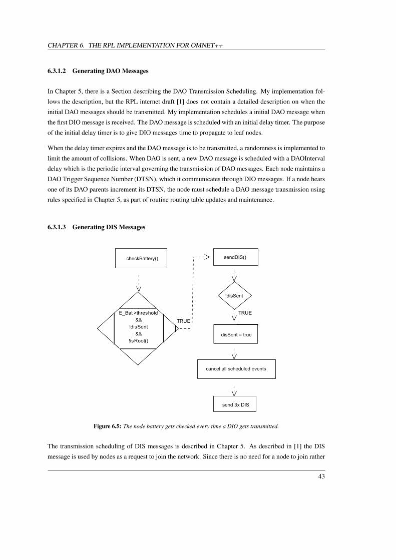
CHAPTER 6. THE RPL IMPLEMENTATION FOR OMNET++
6.3.1.2 Generating DAO Messages
In Chapter 5, there is a Section describing the DAO Transmission Scheduling. My implementation fol-
lows the description, but the RPL internet draft [1] does not contain a detailed description on when the
initial DAO messages should be transmitted. My implementation schedules a initial DAO message when
the first DIO message is received. The DAO message is scheduled with an initial delay timer. The purpose
of the initial delay timer is to give DIO messages time to propagate to leaf nodes.
When the delay timer expires and the DAO message is to be transmitted, a randomness is implemented to
limit the amount of collisions. When DAO is sent, a new DAO message is scheduled with a DAOInterval
delay which is the periodic interval governing the transmission of DAO messages. Each node maintains a
DAO Trigger Sequence Number (DTSN), which it communicates through DIO messages. If a node hears
one of its DAO parents increment its DTSN, the node must schedule a DAO message transmission using
rules specified in Chapter 5, as part of routine routing table updates and maintenance.
6.3.1.3 Generating DIS Messages
Figure 6.5: The node battery gets checked every time a DIO gets transmitted.
The transmission scheduling of DIS messages is described in Chapter 5. As described in [1] the DIS
message is used by nodes as a request to join the network. Since there is no need for a node to join rather
43
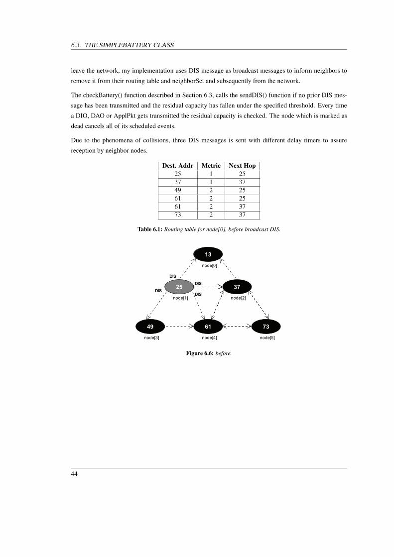
6.3. THE SIMPLEBATTERY CLASS
leave the network, my implementation uses DIS message as broadcast messages to inform neighbors to
remove it from their routing table and neighborSet and subsequently from the network.
The checkBattery() function described in Section 6.3, calls the sendDIS() function if no prior DIS mes-
sage has been transmitted and the residual capacity has fallen under the specified threshold. Every time
a DIO, DAO or ApplPkt gets transmitted the residual capacity is checked. The node which is marked as
dead cancels all of its scheduled events.
Due to the phenomena of collisions, three DIS messages is sent with different delay timers to assure
reception by neighbor nodes.
Dest. Addr Metric Next Hop25 1 2537 1 3749 2 2561 2 2561 2 3773 2 37
Table 6.1: Routing table for node[0], before broadcast DIS.
736149
3725
13
Figure 6.6: before.
44

CHAPTER 6. THE RPL IMPLEMENTATION FOR OMNET++
Dest. Addr Metric Next Hop37 1 3761 2 3773 2 3749 3 37
Table 6.2: Routing table for node[0], after broadcast DIS.
7361
49
3725
13
Figure 6.7: after.
In Figure 6.6 node 1 reaches its battery threshold and sends a broadcast DIS indicating it has no more
power left. The routing table of the root node is displayed before and after DIS transmission/reception.
In Figure 6.7 the neighbors of the node 1 receives the DIS message and cleans their table, removing node
1.
45
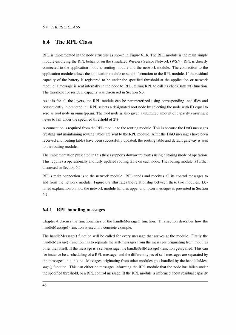
6.4. THE RPL CLASS
6.4 The RPL Class
RPL is implemented in the node structure as shown in Figure 6.1b. The RPL module is the main simple
module enforcing the RPL behavior on the simulated Wireless Sensor Network (WSN). RPL is directly
connected to the application module, routing module and the network module. The connection to the
application module allows the application module to send information to the RPL module. If the residual
capacity of the battery is registered to be under the specified threshold at the application or network
module, a message is sent internally in the node to RPL, telling RPL to call its checkBattery() function.
The threshold for residual capacity was discussed in Section 6.3.
As it is for all the layers, the RPL module can be parameterized using corresponding .ned files and
consequently in omnetpp.ini. RPL selects a designated root node by selecting the node with ID equal to
zero as root node in omnetpp.ini. The root node is also given a unlimited amount of capacity ensuring it
never to fall under the specified threshold of 2%.
A connection is required from the RPL module to the routing module. This is because the DAO messages
creating and maintaining routing tables are sent to the RPL module. After the DAO messages have been
received and routing tables have been successfully updated, the routing table and default gateway is sent
to the routing module.
The implementation presented in this thesis supports downward routes using a storing mode of operation.
This requires a operationally and fully updated routing table on each node. The routing module is further
discussed in Section 6.5.
RPL’s main connection is to the network module. RPL sends and receives all its control messages to
and from the network module. Figure 6.8 illustrates the relationship between these two modules. De-
tailed explanation on how the network module handles upper and lower messages is presented in Section
6.7.
6.4.1 RPL handling messages
Chapter 4 discuss the functionalities of the handleMessage() function. This section describes how the
handleMessage() function is used in a concrete example.
The handleMessage() function will be called for every message that arrives at the module. Firstly the
handleMessage() function has to separate the self-messages from the messages originating from modules
other then itself. If the message is a self-message, the handleSelfMessage() function gets called. This can
for instance be a scheduling of a RPL message, and the different types of self-messages are separated by
the messages unique kind. Messages originating from other modules gets handled by the handleInMes-
sage() function. This can either be messages informing the RPL module that the node has fallen under
the specified threshold, or a RPL control message. If the RPL module is informed about residual capacity
46
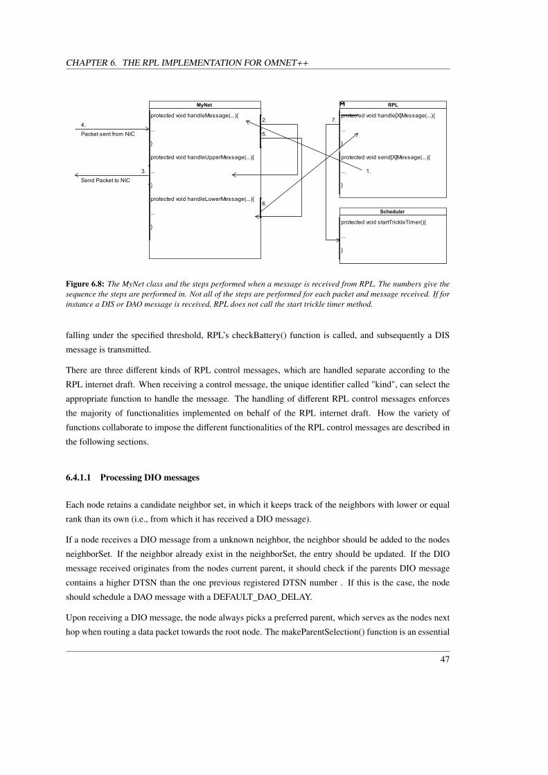
CHAPTER 6. THE RPL IMPLEMENTATION FOR OMNET++
MyNet RPL
Scheduler
Figure 6.8: The MyNet class and the steps performed when a message is received from RPL. The numbers give thesequence the steps are performed in. Not all of the steps are performed for each packet and message received. If forinstance a DIS or DAO message is received, RPL does not call the start trickle timer method.
falling under the specified threshold, RPL’s checkBattery() function is called, and subsequently a DIS
message is transmitted.
There are three different kinds of RPL control messages, which are handled separate according to the
RPL internet draft. When receiving a control message, the unique identifier called "kind", can select the
appropriate function to handle the message. The handling of different RPL control messages enforces
the majority of functionalities implemented on behalf of the RPL internet draft. How the variety of
functions collaborate to impose the different functionalities of the RPL control messages are described in
the following sections.
6.4.1.1 Processing DIO messages
Each node retains a candidate neighbor set, in which it keeps track of the neighbors with lower or equal
rank than its own (i.e., from which it has received a DIO message).
If a node receives a DIO message from a unknown neighbor, the neighbor should be added to the nodes
neighborSet. If the neighbor already exist in the neighborSet, the entry should be updated. If the DIO
message received originates from the nodes current parent, it should check if the parents DIO message
contains a higher DTSN than the one previous registered DTSN number . If this is the case, the node
should schedule a DAO message with a DEFAULT_DAO_DELAY.
Upon receiving a DIO message, the node always picks a preferred parent, which serves as the nodes next
hop when routing a data packet towards the root node. The makeParentSelection() function is an essential
47
6.4. THE RPL CLASS
piece of the RPL implementation. Therefore an own section is devoted to explain its functionalities, see
section 6.4.1.4. The parent selection function is selected depending on the metric used in the DODAG
structure.
In the case of the first received DIO message, the node starts its trickle timer which periodically emits
DIO message governed by rules described Section 5.3.3.1 and implemented as shown in Section 6.8.
Figure 6.4 displays the transmission of DIO message after receiving the initial DIO message from the
root node. A DAO message is scheduled as described in Section 6.3.1.2.
If the node receiving a DIO message is the root node, or a node marked as dead, the DIO message should
be deleted to prevent further processing. The boolean value isDead is set as true when a node transmits
a DIS message. This avoids transmission from a "dead" node, subsequently including it back into the
network topology.
48
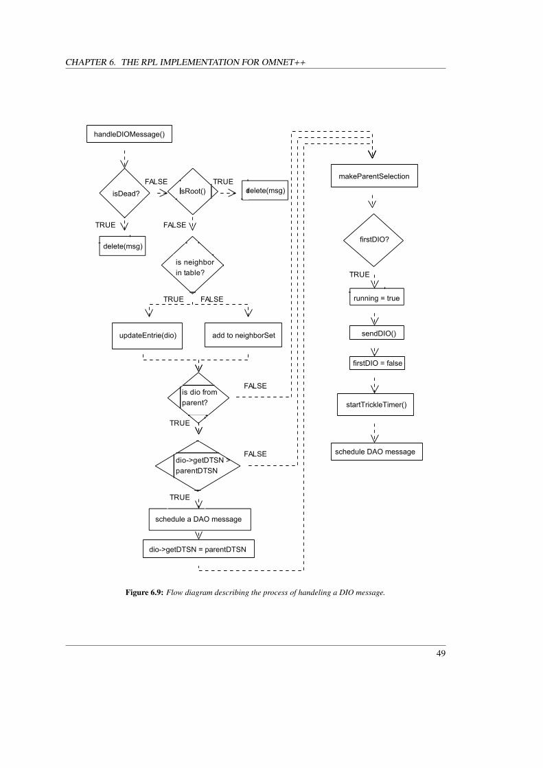
CHAPTER 6. THE RPL IMPLEMENTATION FOR OMNET++
Figure 6.9: Flow diagram describing the process of handeling a DIO message.
49
6.4. THE RPL CLASS
6.4.1.2 Processing DAO messages
When receiving a DAO message, the only difference in handling the message for a regular node compared
to the root node is the makeParentSelection() function. Obviously, the root node does not select a parent,
since it is the ultimate node itself. A regular node should select a preferred parent to which it should send
its updated DAO message. In order to maximize the chances to perform route aggregation, the DAO mes-
sage toward its parent is delayed using a delayDAO timer. The default value is DEFAULT_DAO_DELAY,
which has a value of 1 second.
The node retrives information included in the received DAO message and adds it to its routing table
using functions addNeighborToRoutingTable() and addRoutesToRoutingTable(). Both function uses the
information received in the DAO message to add or update routing entries.
The process of updating the DAO message begins with the addNeighborToRoutingTable() function. This
function starts by adding information about the sender in a Routeinfo object. This Routeinfo object is
then checked up against the routes currently stored in the routing table. To avoid double entries, a route
that already exist in the routing table should not be added, but can be updated if it conains new metric
value. New routes should be added to the routing table using the addRoutesToRoutingTable() function.
The addRoutesToRoutingTable() function iterates trough the received routing table, adding new routes.
Accordingly, the updated routing table is sent to the Routing module.
The first DAO message received at each node schedules a increase of DTSN flag used as part of the
procedure to maintain downward routes. The increment of the DTSN flag is delayed with a default value
DTSN_DELAY, which has a value of 15 second.
Like the processing of DIO messages, the handleDAOMessage() starts by checking if the node receiving
the DAO message isDead, and deleting the message if it is.
50

CHAPTER 6. THE RPL IMPLEMENTATION FOR OMNET++
Figure 6.10: Flow diagram describing the process of handling a DAO message.
51

6.4. THE RPL CLASS
6.4.1.3 Processing DIS messages
Upon receiving a DIS message from a neighbor, the dead node needs to be removed from the receiving
nodes neighborSet and routing table. All nodes, except the root node, needs to make a new parent se-
lection in case the dead node were the previous parent. The node also has to reset its trickle timer to the
minimum value of I_min, shortening the time to the next spontaneous DIO transmission. This is desir-
able to inform the network about the topology changes. At last the routing tables are sent from all nodes
receiving a DIS message.
Figure 6.11: The node battery gets checked every time a DIO, DAO and ApplPkt gets transmitted.
6.4.1.4 The makeParentSelection function
When the nodes neighborSet is successfully populated, it contains information about the neighbors rank,
source address and metric. The makeParentSelection() function uses these variables in a strict set of rules
listed below, to determine which neighbor should be selected preferred parent. If the metric used is hop
count there are two criteria for selecting a parent.
1. When selecting a parent, the first criteria is rank. The node iterates trough its neighborSet searching
for the neighbor with the lowest rank.
2. The second criteria is source address. If the node discovers more than one potential parent using
the first criteria, the node with the lowest source address is selected parent.
If the metric used in the simulation is node energy the information stored in the metric field is taken into
account.
52

CHAPTER 6. THE RPL IMPLEMENTATION FOR OMNET++
1. Like hop count, the first criteria for selecting a parent is rank. The node iterates trough its neigh-
borSet searching for the neighbor with the lowest rank.
2. The second criteria is node energy. If the node discovers more than one potential parent using the
first criteria, the node selects the neighbor with highest percentage of battery capacity remaining.
3. The third criteria is source address. If the node discovers more than one potential parent using the
first and the second criteria, the node with the lowest source address is selected parent.
When a preferred parent is selected, the node uses its parents rank to calculate its own (prarent-rank+1).
In the scenario where the traffic is sent towards the root node, DIO message from a parent gives a node
information about the battery status. In other words, the node needs to receive a DIO message in order to
trigger the selection of parent. The effects this has on the simulation results will be further discussed in
the next chapter.
53

6.5. THE ROUTING CLASS
6.5 The Routing Class
The Routing module implements the internal routing table used by RPL storing mode of operation. In
storing mode, all non-root, non-leaf nodes MUST store routing table entries for destinations learned from
DAOs.
The routing table and default gateway could have been stored directly in the RPL module, eliminating the
need for a routing module. This would result in a larger amount of messages arriving at the RPL module,
as the messages would pass through the RPL module for routing. To provide a more tidy implementation,
a separate module for routing were created, moving some of the functionalities away from the RPL
module.
The Routing module is directly connected to the RPL module and the network module interacting using
internal messages. The Routing module contains a routing table and a default gateway, advertised by
RPL. The default gateway contains a RouteInfo object made up of a destination address, metric and next
hop of the current parent. The default gateway is maintained using the makeParentSelection() function
described in section 6.4.1.4.
54

CHAPTER 6. THE RPL IMPLEMENTATION FOR OMNET++
Dest. Addr Metric Next Hop37 1 3761 2 3773 2 3749 3 37
Table 6.3: A routing table example taken from Table 6.2.
The routing table is a vector of RouteInfo objects. Table 6.3 displays how the vector of RouteInfo ob-
jects can function as a routing table. There are rows of RouteInfo objects and columns of variables the
RouteInfo objects consist of.
RPL creates and maintains routing tables using unicast DAO messages. DAO messages are periodically
emitted using the DAOInterval, and are also triggered by parents incrementing its DTSN value (advertised
using DIO messages). Prior to each DAO transmission, the node’s routing table is sent (internally in the
node) to the Routing module. The routing table is sent using a sendRoutingTable() function, described in
the section below.
The network module uses the routing module in the process of selecting paths in a network along which to
send network traffic. RPL control messages does not use the routing module when forwarding traffic. In
storing mode the DAO message is unicast by the child to the selected parent. The address to the selected
parent is added when sending the DAO message, and since the destination is only one hop away, routing
is not required. DIO and DIS message are always sent as a broadcast message without a specified L3
destination address.
An application packet is unicast with a specified L3 destination network address. The network module
forwards messages the application packet to the routing module if a next hop towards destination is
required. If a application packet is received at the routing module, a iteration trough the routing table is
done searching for a matching routing entry providing a next hop towards destination. In the case where
redundant paths are found, the preferable path according to the current metric is chosen, and set as next
hop. When no matching routing entries are found, the default gateway is used as next hop towards the
destination. When the next hop is selected, the message is returned back out to the network module.
As it is for all the modules, the routing module can be parameterized using corresponding .ned files and
consequently in omnetpp.ini.
6.5.0.5 Routing Table Message
The routing table is maintained using DAO messages communicated by the RPL module. In order to send
updated routing tables to the Routing module, a sendRoutingTable() function was created.
The sendRoutingTable() function creates a messages using the PktRPL_m class. The message updates
the routing table and default gateway before transmission. As the message only gets sent internally in
55

6.5. THE ROUTING CLASS
the node (i.e. from the RPL module to the Routing module) it does not have any impact on the battery
consumption according to the specification of this implementation. The process of packing a class vector
into a message is complicated. Appendix A contains the code. When receiving the routing table message,
the Routing module unpacks the information stored in the message and adds it to its own routing table
and default gateway.
56

CHAPTER 6. THE RPL IMPLEMENTATION FOR OMNET++
6.6 The TestApplication Class
The TestApplication is part of the hierarchical layers represented by the modules in 6.1b interacting using
internal messages. The application layer is implemented to provoke behavior desirable for measurements
to be made. For instance, measurements of network lifetime requires application packets to be sent
frequently in order to drain nodes for battery until every single node in the network is dead. The messages
from lower layers are processed in event void TestApplication::handleLowerMsg(cMessage*msg) where
TestApplication is the name of my tailord version of TestApplication. The packets are sent using function
sendDown(pkt) where pkt is the packet created in the application layer. The packet is passed to network
layer for further processing. The process of passing messages continues until the packet reaches physical
layer. Then it can be sent using communication module. The TestApplication module provided by MiXiM
was re-implemented to function according to my requirements. As it is for all the layers, the applications
can be parameterized using corresponding .ned files and consequently in omnetpp.ini.
The application layer is a higher layer module connected to the RPL module and the network module
as displayed in Figure 6.1b. Like the RPL module, the application layer has a checkBattery() function
which is called each time an application packet is sent. The connection between the application and
RPL module is used by the application module to warn RPL if the residual capacity has fallen under the
threshold specified in section 6.3. When RPL receives this message, RPL is prompted to call its own
checkBattery() function, subsequently sending a broadcast DIS message.
6.6.1 Traffic Flows
For this implementation, two kinds of traffic flows are examined. Upward traffic towards the root node,
and downward traffic from the root node.
When sending upward traffic, every node except for the root node itself sends application packets using
a exponential distribution function. The amount of data sent by each node is equal, and packets uses the
root node’s network address as destination address.
For downward traffic, the root node is the only node sending data. Before every application packet sent,
the root node sets it own network address as source address and selects the receiving node using a uniform
distribution function. When an application packet has reached its destination, it is sent to the application
module where it is registered and deleted.
57

6.7. THE MYNET CLASS
6.7 The MyNet Class
MyNet is an implemented extension to the network layer existing in MiXiM, called BaseNetwLayer.
MyNet supports the handling of RPL control messages, and the connection to the routing module. The
main purpose of the extension is to limit the altering of existing framework modules.
MyNet inherit functions such as decapsMsg() and encapsMsg() which is critical for the handling for
RPL control messages. The network module lies between the implemented modules and the pre-existing
framework modules, shown in Figure 6.1b.
The network module is connected upper modules such as the application module and RPL module. Broad-
cast messages received from upper modules are sent directly down to lower modules after they have been
casted as network packets and encapsulated. Unicast messages gets sent to the routing module to obtain
the next hop towards its destination, then casted to a network packet and encapsulated before being sent
down, after returning from the routing module.
Airframes received at the PHY layer are sent trough the MAC layer up to the network layer. Here, the
network layer de-capsulate the received message, and determines what to do with the message using the
unique identifier "kind" included in the message. RPL control messages are sent to the RPL module, while
the application packets gets sent to the application module if the message has reached its destination.
If not, the message is sent out to the Routing module where it determines the next hop towards the
destination, and finally the message is sent back out from the physical layer as an airframe. The network
also contains an own message informing the RPL module if a node is registered as dead. This message is
casted as a NetwPkt, and is sent internally in the node to the RPL module.
58

CHAPTER 6. THE RPL IMPLEMENTATION FOR OMNET++
6.8 The TrickleTimer Class
The main assumption of Trickle is that when the network is stable (i.e. no changes causing the trickle
timer to reset) less overhead is caused by sending DIO messages. The TrickleTimer class is a subclass
within RPL. This allows it to access all of RPL’s functions and makes it easy to implement. Figure 6.12
displays the implementation of the Trickle algorithm including expository comment.
At initiation, the root node starts its trickle timer, and sends out an initial broadcast DIO message. When
the DIO message arrive at the RPL module of the neighbor nodes, RPL proceeds to perform the steps
shown in Figure 6.4.
/*When the algorithm starts execution, it sets I to a value in the range of [Imin, Imax] -- that is, greater than or equal to Imin and less than or equal to Imax. The algorithm then begins the first interval.*/ void RPL::startTrickleTimer() { I = I_min + rand() % (I_max - I_min); scheduleAt((simTime()+I), triggerDIO); } /*When the interval I expires, Trickle doubles the interval length. If this new interval length would be longer than the time specified by Imax, Trickle sets the interval length I to be the time specified by Imax.*/ void RPL::increaseInterval(){ if(running){ I = I*2; //double the interval if(I>=I_max){ I = I_max; } scheduleAt((simTime()+I), triggerDIO); } } /*If Trickle hears a transmission that is "inconsistent" (i.e. a DIS message) and I is greater than Imin, it resets the Trickle timer. To reset the timer, Trickle sets I to Imin and starts a new interval.*/ void RPL::resetTrickleTimer() { I = I_min; //reset the interval to I_min. cancelEvent(resetDIO); cancelEvent(triggerDIO); scheduleAt((simTime()+I), resetDIO); }
Figure 6.12: An implementation of the Trickle algorithm in C++.
The resetTrickleTimer() function gets called if a node receives a DIS message. The resetTrickleTimer()
function schedules a DIO message with a interval equal to I_min. When the interval expires, the handle-
SelfMessage() function is called returning us to step. 6 in Figure 6.4.
59
6.9. EVALUATED METRICS
6.9 Evaluated Metrics
The implementation presented in this paper implements two different metrics; hop count and node en-
ergy. The purpose is to compare and evaluate the variation of power consumed when using the different
metric. When running the simulation, a decision is prompted where the user has to select which is to be
used.
6.9.1 Node Energy Object
The implementation of the node energy object is using the mid-complexity solution presented in ??. In
the configuration file omnetpp.ini every node except the root node is given the exact same total capacity.
For battery powered devices, E-E is the ratio of desired max power to actual power, E-E=P_max/P_now,
in units of percent.
The node energy object uses the percentage of remaining energy as metric. Figure x illustrates how a
path decision is done using percentage of residual capacity as Object Function (OF). In addition, the node
energy object uses its own version of makeParentSelection() function described in Section 6.4.1.4.
Before a DAO message is sent, the current percentage of remaining energy has to be replaced with the
old. This is done using a function correctingRoutingTable() which makes a copy of the previous routing
table (correctedRoutingTable) and iterating trough it, replacing every E-E value lower than the current
E-E value. Finally the correctedRoutingTable is set as the routing table, and the DAO message gets
transmitted.
6.9.2 Hop Count
The implementation of hop count was pretty straight forward. When a node receives a routing table from
a child, it selects the routes not previously stored in its routing table and updates the others if needed.
When storing the node sending the DAO as well as the routing table it contains, all entries metric is
incremented by 1.
60

CHAPTER 6. THE RPL IMPLEMENTATION FOR OMNET++
6.10 Output
The finish() function is for recording statistics, and it only gets called when the simulation has terminated
normally. It does not get called when the simulations stops with an error message.
In order to record capacity or table size on a node over time, a vector were created of class OutputInfo. A
self message was used to store the simulation time and the residual capacity in the vector every second.
At the finish() function an iterator was used recover the elements in the vector and write it to the output
.sca file.
To record nodes dying, a simtime_t object was created were the time of death was registered and recorded
at the finish() function.
The output registered by the finish function is stored in a .sca file. a Java program was created to filter out
the desired data from the output. The desired data was stored in a .txt file readable for Gnuplot.
61
Chapter 7
RESULTS AND ANALYSIS
This chapter describes and analyzes the results of the simulations conducted in this thesis.
If not otherwise specified, the data traffic flows from all nodes towards the root node. Data traffic orig-
inates at the application layer, and is sent continuously from all nodes with a random delay. The node
topologies differ depending on the simulation, and will be described where necessary. Table 7.1 lists other
key default parameters used in the simulation.
Parameter ValueMode of operation Storing
Rank Metric Hop Count/Node EnergyDIOIntervalDoublings 16
DIOIntervalMin 1 secDIOIntervalMax 5sec
DAOInterval 5 sec
Table 7.1: Parameters in simulation.
7.1 Simulation Issues
This section will describe how the RPL protocol, having an area of application developed for a real time
deployment, affects the simulation. Implementation limitations to the simulation is also discussed.
7.1.1 Simulation compared to real time deployment
Table 7.2 lists the battery parameters used in the simulation, if not otherwise specified. Runtime in
OMNeT++ was taken into consideration while selecting values for battery capacity in the simulation. To
62

CHAPTER 7. RESULTS AND ANALYSIS
keep the simulation time within a reasonable limit, realistic battery capacity values obtained from real
time deployment(s), could not be used.
Parameter ValueNominal Battery Capacity 3000 mA
Battery Capacity 3000 mANominal Voltage 3 V
Table 7.2: Battery parameters in simulation.
The implementation presented in this thesis, node energy metric requires a continuous updating of the
battery capacity. Using the node energy metric, node(s) update battery capacity in their neighbor set
each time they receive a DIO message. The update in battery capacity would subsequently cause child
nodes to swap parent frequently (i.e. always selecting the candidate parent with the highest residual
capacity).
In a real time deployment, the trickle timer would govern the transmission intensity of DIO messages,
using a maximum interval described in Section 5.3.3.1.2. The interval between DIO transmissions would
eventually reach a maximum interval equal to 18.2 hours, under a steady network condition. The lifetime
of the sensor nodes in a real time deployment is a high as 2 months, with a expected lifetime of one
year [13]. To determine the frequency of DIO transmissions/receptions in a worst case scenario, the
total lifetime of the nodes is divided by the amount of DIO messages transmitted using the maximum
interval.
The lifetime of sensor nodes in my simulation is in the order of 5-20 minutes. To obtain an equally
frequent reception of DIO messages in the simulation, DIOIntervalMax must be decreased. Subse-
quently this influences the behavior of the trickle timer as the exponential increase from DIOIntervalMin
to DIOIntervalMax only consist of a minimal number of interval doublings.
7.1.2 Simulation without RX state
As described in Section 6.3, the RX state was not included in simulations due to its overrated power
consumption in the absence of the IDLE state.
The simulation is nevertheless valid for the special WSN, where the nodes are synchronized. This syn-
chronization allows only recipient nodes to forward traffic. In other words, there is no traffic transmitted
by nodes unless they receive traffic themselves.
63

7.2. POWER DRAINED FROM NODES AT RANK 1
7.2 Power drained from nodes at rank 1
Nodes close to the sink must support more loads than nodes further away from the sink. In this section a
special configuration of nodes was designed. The motivation was to investigate the power dissipation of
the nodes close to the sink for the two alternative metrics.
Figure 7.1: Special configuration of nodes, examining power drained from nodes at rank 1.
Figure 7.1 displays a network topology where the root node (at the top of the topology) is connected to
three nodes. These nodes handle traffic from the entire network below. The purpose of this structure is
to assess how the traffic is divided among these three nodes, using the two metrics of interest: Hop count
64

CHAPTER 7. RESULTS AND ANALYSIS
and node energy.
From our knowledge of how the hop count metric selects parents as described in Section 6.4.1.4, it is
reasonable to assume that the node with the lowest source address will be selected parent.
0
500
1000
1500
2000
2500
3000
0 50 100 150 200 250 300 350 400 450
node
cap
acity
(m
A)
time (s)
Node[1]Node[2]Node[3]
Figure 7.2: Power drained from nodes at rank 1, using Hop Count.
Figure 7.2 shows the battery capacity during simulation for the three nodes with rank equal 1 seen in
topology-figure 7.1, i.e. node 1, 2 and 3. Note that the metric used is hop count. As anticipated, the child
nodes will first choose node 1 due to its low id (node 1,2,3 all have identical hop count towards the root)
as its parent. This will strain the battery of node 1 and cause the steep decline in battery capacity as seen
in the Figure 7.3.
After approximately 160 seconds, node 1 has exhausted its battery. Node 1 triggers a broadcast DIS
message, announce that it has no more power left. This will trigger the child nodes to elect a new parent,
i.e. the node with the second lowest id: Node 2. At approximately 300 seconds, node 2 has exhausted its
battery. Node 2 will send out a DIS message, and the child nodes will select Node 3 as its parent. When
Node 3 reaches zero capacity, there is no connection from the network towards the root.
Using hop count as a metric consequently causes the child nodes to choose one common parent and utilize
it until its energy is depleted. This has a negative impact on the network, since some child nodes may
only reach the root through this node. These child nodes will lose connectivity, while other nodes may
select a new parent.
Figure 7.3 shows an identical network, while using node energy. As anticipated, the child nodes will
65
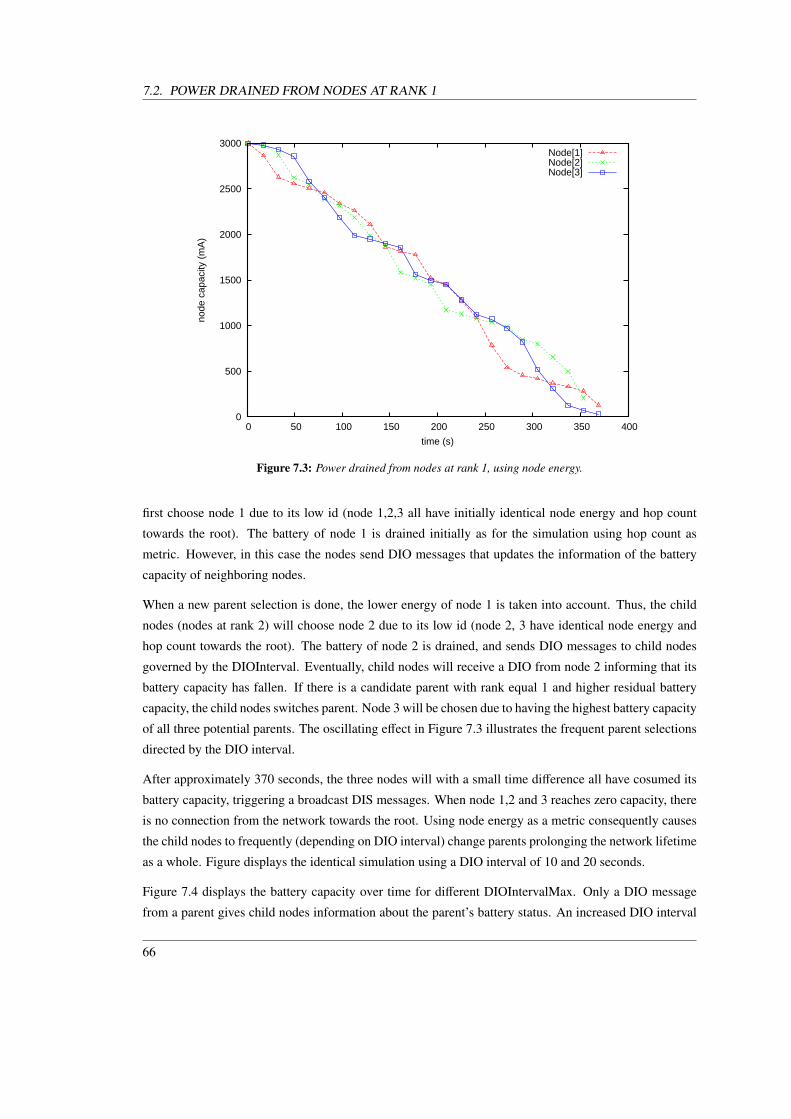
7.2. POWER DRAINED FROM NODES AT RANK 1
0
500
1000
1500
2000
2500
3000
0 50 100 150 200 250 300 350 400
node
cap
acity
(m
A)
time (s)
Node[1]Node[2]Node[3]
Figure 7.3: Power drained from nodes at rank 1, using node energy.
first choose node 1 due to its low id (node 1,2,3 all have initially identical node energy and hop count
towards the root). The battery of node 1 is drained initially as for the simulation using hop count as
metric. However, in this case the nodes send DIO messages that updates the information of the battery
capacity of neighboring nodes.
When a new parent selection is done, the lower energy of node 1 is taken into account. Thus, the child
nodes (nodes at rank 2) will choose node 2 due to its low id (node 2, 3 have identical node energy and
hop count towards the root). The battery of node 2 is drained, and sends DIO messages to child nodes
governed by the DIOInterval. Eventually, child nodes will receive a DIO from node 2 informing that its
battery capacity has fallen. If there is a candidate parent with rank equal 1 and higher residual battery
capacity, the child nodes switches parent. Node 3 will be chosen due to having the highest battery capacity
of all three potential parents. The oscillating effect in Figure 7.3 illustrates the frequent parent selections
directed by the DIO interval.
After approximately 370 seconds, the three nodes will with a small time difference all have cosumed its
battery capacity, triggering a broadcast DIS messages. When node 1,2 and 3 reaches zero capacity, there
is no connection from the network towards the root. Using node energy as a metric consequently causes
the child nodes to frequently (depending on DIO interval) change parents prolonging the network lifetime
as a whole. Figure displays the identical simulation using a DIO interval of 10 and 20 seconds.
Figure 7.4 displays the battery capacity over time for different DIOIntervalMax. Only a DIO message
from a parent gives child nodes information about the parent’s battery status. An increased DIO interval
66

CHAPTER 7. RESULTS AND ANALYSIS
0
500
1000
1500
2000
2500
3000
0 50 100 150 200 250 300 350 400 450
node
cap
acity
(m
A)
time (s)
Node[1]Node[2]Node[3]
(a) 10 sec
0
500
1000
1500
2000
2500
3000
0 50 100 150 200 250 300 350 400 450
node
cap
acity
(m
A)
time (s)
Node[1]Node[2]Node[3]
(b) 20 sec
Figure 7.4: Battery capacity over time for different DIOIntervalMax.
will therefore subsequently cause the child to swap parents less frequent.
Figure 7.4a displays the battery capacity over time using a DIOIntervalMax equal 10 seconds. The first
increased DIO transmission interval causes the frequency of parent selections to decrease, illustrated
by the oscillation shown in Figure 7.4a. The irregularities in the oscillation can be explained by DIO
messages collations. If a DIO message from a parent does not arrive to update the residual battery
capacity, the parent swap can be delayed.
Figure 7.4b displays the battery capacity over time using a DIOIntervalMax equal 20 seconds. The
second increased DIO transmission interval causes the frequency of parent selections to decrease even
more, illustrated by the oscillation shown in Figure 7.4a. As described above, the irregularities in the
oscillation can be explained by DIO messages collations.
67

7.3. SPECIAL NETWORK WITH SUB-NETWORKS
7.3 Special network with sub-networks
This section also investigates a special network configuration. Nodes in the network which are the only
"physical" connection between larger group of nodes and the root node. The motivation was to investigate
the power dissipation of the nodes connecting these groups.
Figure 7.5 displays a network topology divided into three main "sub-networks". The left "sub-network"
maintaining a path towards the root node solely trough node 4. The right "sub-network" maintaining a
path towards the root node solely trough node 5. And, finally the central "sub-network" connected the
root node though all nodes with rank equal to 2.
The purpose of this topology is to measure battery consumption on nodes with rank equal to 2 (i.e. node
4,5,6,7 and 8) using the metrics of interest: hop count and node energy.
Figure 7.5: Special network configuration, examining nodes connecting parts of the network to rest of the networktopology containing the root node.
Figure 7.6 shows the battery capacity during simulation for the five nodes with rank equal 2, seen in
topology-figure 7.5. Note that the metric used is hop count. The two outer "sub-networks" will select
68
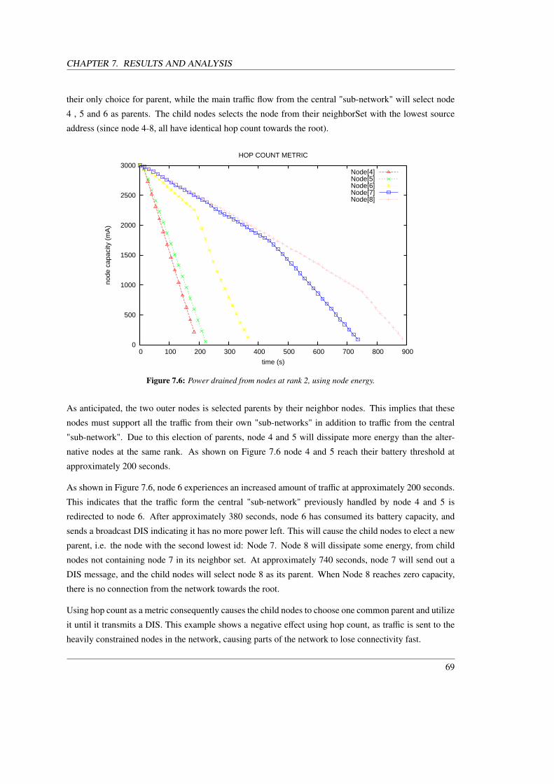
CHAPTER 7. RESULTS AND ANALYSIS
their only choice for parent, while the main traffic flow from the central "sub-network" will select node
4 , 5 and 6 as parents. The child nodes selects the node from their neighborSet with the lowest source
address (since node 4-8, all have identical hop count towards the root).
0
500
1000
1500
2000
2500
3000
0 100 200 300 400 500 600 700 800 900
node
cap
acity
(m
A)
time (s)
HOP COUNT METRIC
Node[4]Node[5]Node[6]Node[7]Node[8]
Figure 7.6: Power drained from nodes at rank 2, using node energy.
As anticipated, the two outer nodes is selected parents by their neighbor nodes. This implies that these
nodes must support all the traffic from their own "sub-networks" in addition to traffic from the central
"sub-network". Due to this election of parents, node 4 and 5 will dissipate more energy than the alter-
native nodes at the same rank. As shown on Figure 7.6 node 4 and 5 reach their battery threshold at
approximately 200 seconds.
As shown in Figure 7.6, node 6 experiences an increased amount of traffic at approximately 200 seconds.
This indicates that the traffic form the central "sub-network" previously handled by node 4 and 5 is
redirected to node 6. After approximately 380 seconds, node 6 has consumed its battery capacity, and
sends a broadcast DIS indicating it has no more power left. This will cause the child nodes to elect a new
parent, i.e. the node with the second lowest id: Node 7. Node 8 will dissipate some energy, from child
nodes not containing node 7 in its neighbor set. At approximately 740 seconds, node 7 will send out a
DIS message, and the child nodes will select node 8 as its parent. When Node 8 reaches zero capacity,
there is no connection from the network towards the root.
Using hop count as a metric consequently causes the child nodes to choose one common parent and utilize
it until it transmits a DIS. This example shows a negative effect using hop count, as traffic is sent to the
heavily constrained nodes in the network, causing parts of the network to lose connectivity fast.
69
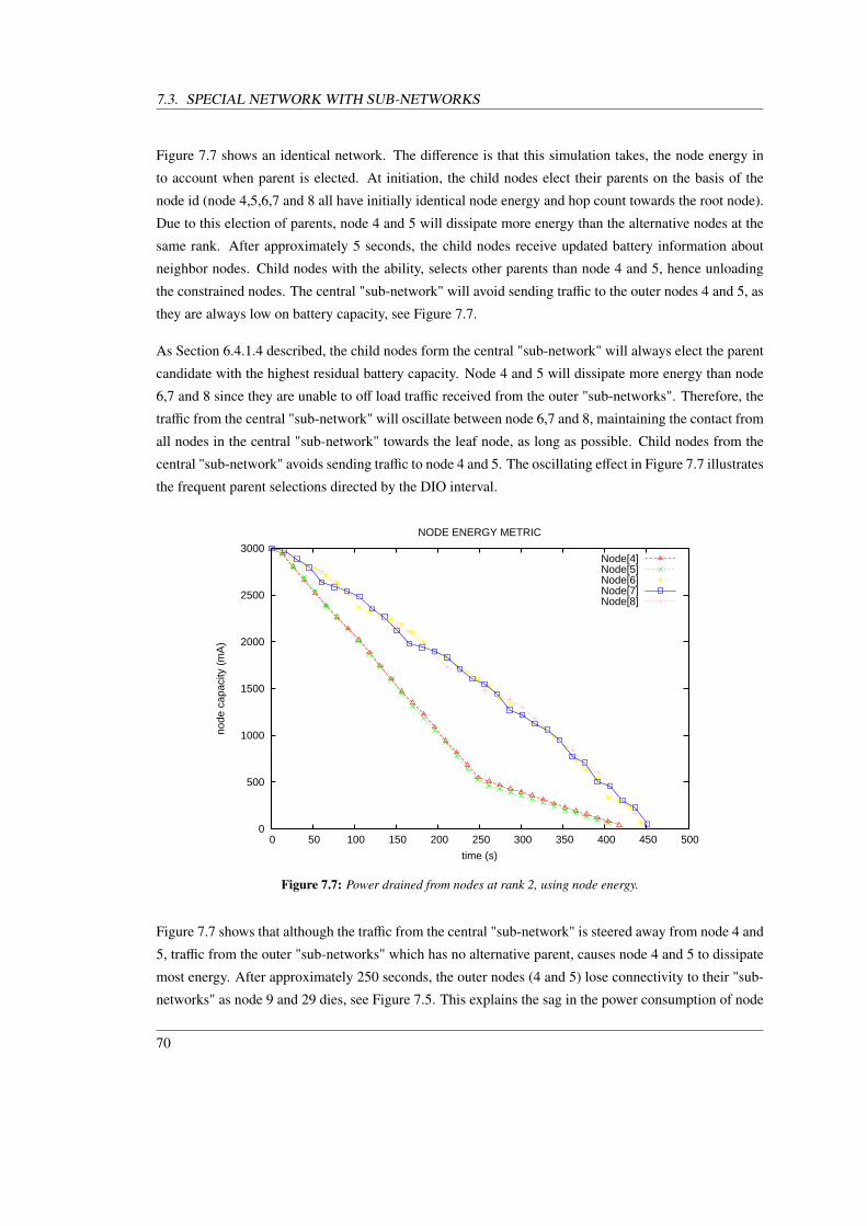
7.3. SPECIAL NETWORK WITH SUB-NETWORKS
Figure 7.7 shows an identical network. The difference is that this simulation takes, the node energy in
to account when parent is elected. At initiation, the child nodes elect their parents on the basis of the
node id (node 4,5,6,7 and 8 all have initially identical node energy and hop count towards the root node).
Due to this election of parents, node 4 and 5 will dissipate more energy than the alternative nodes at the
same rank. After approximately 5 seconds, the child nodes receive updated battery information about
neighbor nodes. Child nodes with the ability, selects other parents than node 4 and 5, hence unloading
the constrained nodes. The central "sub-network" will avoid sending traffic to the outer nodes 4 and 5, as
they are always low on battery capacity, see Figure 7.7.
As Section 6.4.1.4 described, the child nodes form the central "sub-network" will always elect the parent
candidate with the highest residual battery capacity. Node 4 and 5 will dissipate more energy than node
6,7 and 8 since they are unable to off load traffic received from the outer "sub-networks". Therefore, the
traffic from the central "sub-network" will oscillate between node 6,7 and 8, maintaining the contact from
all nodes in the central "sub-network" towards the leaf node, as long as possible. Child nodes from the
central "sub-network" avoids sending traffic to node 4 and 5. The oscillating effect in Figure 7.7 illustrates
the frequent parent selections directed by the DIO interval.
0
500
1000
1500
2000
2500
3000
0 50 100 150 200 250 300 350 400 450 500
node
cap
acity
(m
A)
time (s)
NODE ENERGY METRIC
Node[4]Node[5]Node[6]Node[7]Node[8]
Figure 7.7: Power drained from nodes at rank 2, using node energy.
Figure 7.7 shows that although the traffic from the central "sub-network" is steered away from node 4 and
5, traffic from the outer "sub-networks" which has no alternative parent, causes node 4 and 5 to dissipate
most energy. After approximately 250 seconds, the outer nodes (4 and 5) lose connectivity to their "sub-
networks" as node 9 and 29 dies, see Figure 7.5. This explains the sag in the power consumption of node
70
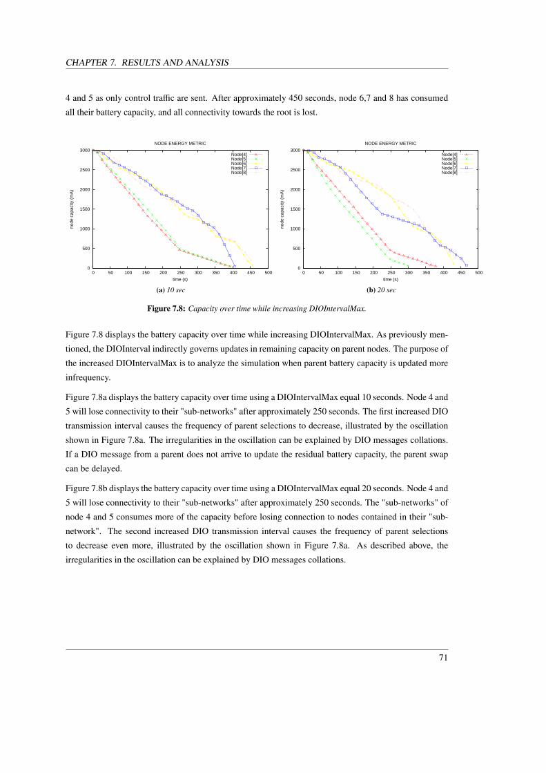
CHAPTER 7. RESULTS AND ANALYSIS
4 and 5 as only control traffic are sent. After approximately 450 seconds, node 6,7 and 8 has consumed
all their battery capacity, and all connectivity towards the root is lost.
0
500
1000
1500
2000
2500
3000
0 50 100 150 200 250 300 350 400 450 500
node
cap
acity
(m
A)
time (s)
NODE ENERGY METRIC
Node[4]Node[5]Node[6]Node[7]Node[8]
(a) 10 sec
0
500
1000
1500
2000
2500
3000
0 50 100 150 200 250 300 350 400 450 500
node
cap
acity
(m
A)
time (s)
NODE ENERGY METRIC
Node[4]Node[5]Node[6]Node[7]Node[8]
(b) 20 sec
Figure 7.8: Capacity over time while increasing DIOIntervalMax.
Figure 7.8 displays the battery capacity over time while increasing DIOIntervalMax. As previously men-
tioned, the DIOInterval indirectly governs updates in remaining capacity on parent nodes. The purpose of
the increased DIOIntervalMax is to analyze the simulation when parent battery capacity is updated more
infrequency.
Figure 7.8a displays the battery capacity over time using a DIOIntervalMax equal 10 seconds. Node 4 and
5 will lose connectivity to their "sub-networks" after approximately 250 seconds. The first increased DIO
transmission interval causes the frequency of parent selections to decrease, illustrated by the oscillation
shown in Figure 7.8a. The irregularities in the oscillation can be explained by DIO messages collations.
If a DIO message from a parent does not arrive to update the residual battery capacity, the parent swap
can be delayed.
Figure 7.8b displays the battery capacity over time using a DIOIntervalMax equal 20 seconds. Node 4 and
5 will lose connectivity to their "sub-networks" after approximately 250 seconds. The "sub-networks" of
node 4 and 5 consumes more of the capacity before losing connection to nodes contained in their "sub-
network". The second increased DIO transmission interval causes the frequency of parent selections
to decrease even more, illustrated by the oscillation shown in Figure 7.8a. As described above, the
irregularities in the oscillation can be explained by DIO messages collations.
71

7.4. STATISTICAL ANALYZE OF NETWORK LIFETIME.
7.4 Statistical Analyze of Network Lifetime.
In this section a statistical analyze of network lifetime is described. The purpose is to provide a more
accurate assumption of how the traffic forwarding choices made by the metrics of interest (i.e. hop count
and node energy) influence the network lifetime.
Figure 7.9 displays a network structure with 120 nodes randomly placed on the playground. The purpose
of the simulation is to analyze the pattern of nodes running out of battery capacity using: hop count and
node energy. In order to conduct a more accurate statistical result of the distribution, ten different network
structures with 120 nodes (randomly placed in its playground size) were created.
Java was applied to create a program generating the different network structures. The network structures
was conducted so as the topology could be reused in different simulations. Java was selected due to prior
knowledge about write to/from file using the java language, see Appendix E.
Figure 7.9: 120 node network example used in the statistical analyse.
72

CHAPTER 7. RESULTS AND ANALYSIS
Figure 7.10 shows the nodes running out of battery capacity during simulation, for a single 120 node
network structure. After approximately 60 seconds, the first node runs out of battery capacity. Note that
the metric evaluated is the hop count object. As displayed in Figure 7.10, the network using hop count
has a larger spread in life time than the network where energy is taken into account. Nodes running out
of battery capacity continuously during simulation. After approximately 360 seconds, the lest node runs
out of battery capacity.
While using node energy, the first node runs out of battery capacity after approximately 80 seconds. As
illustrated in Figure 7.10 the network using node energy keeps as many nodes feasible alive as long as
possible. Instead of nodes dying evenly trough the simulation, the network using node energy experience
a major loss of nodes in the interval between 175 and 250 seconds. After approximately 310 seconds, the
lest node (using node energy) runs out of battery capacity.
0
20
40
60
80
100
120
50 100 150 200 250 300 350 400
# of
dea
d no
des
time (s)
Hop CountNode Energy
Figure 7.10: One of ten node structures used when conducting the statistical analyze.
Figure 7.11 displays a bar chart distribution of nodes running out of battery capacity, divided in 25 second
intervals. The bar chart shows the average simulation results from ten different network structures.
Examining the bar charts, it is clear that the network using hop count has a larger spread in life time then
the network where energy is taken into account. Using the node energy metric, the focus is on keeping
as many nodes as possible connected. Hence, avoid sending traffic to constrained nodes unless necessary.
The networks using the node energy object has a peak of nodes dying between approximately 175 and
275 seconds. After approximately 300 seconds (using the node energy object) almost every node in the
network has run out of battery capacity. For hop count on the other hand, the transmission of packets in
73

7.4. STATISTICAL ANALYZE OF NETWORK LIFETIME.
the network does not come to an end before approximately 375 seconds.
If the lifetime of the network is defined as the time until every node in the network has consumed its
battery capacity, the hop count object gives the best result. On the other hand, if the desired effect is
to have the largest amount of nodes, living as long as possible, the node energy gives the best result.
The latter is usually the desired behavior of a WSN. More nodes able to forward traffic gives a higher
probability that communication between the network and the sink is possible. It is fear to assume that hop
count sends traffic, and completely drains primary nodes towards the sink early in the simulation.
0
5
10
15
20
25
30
35
0-2550-75
75-100
100-125
125-150
150-175
175-200
200-225
225-250
250-275
275-300
300-325
325-350
350-375
# of
dea
d no
des
time (s)
Hop CountNode Energy
Figure 7.11: Statistical overview of network lifetime.
74

CHAPTER 7. RESULTS AND ANALYSIS
7.5 Routing Table Size
This section will give an idea of how the connectivity towards the root node is maintained by the network
during simulation. This is accomplished by monitoring the root node’s routing table over time.
Figure 7.12 displays the primary network module for preliminary simulation results. The network con-
tains 80 nodes randomly placed in its playground size.
Figure 7.13 shows the routing table size of the root node during simulation - using hop count and node
energy. Redundant routes are not counted in Figure 7.13. After approximately 10 seconds, the routing
table contains a route to every node in the network.
Figure 7.12: Network topology for preliminary simulation results.
We start by analyzing the root node’s routing table over time, using hop count (displayed by the black
line with rectangular points). As displayed in Figure 7.13, the root node loses over half of its entries after
approximately 90 seconds. Some entries return, as they select a new parent with a direct connection to
the root node or through intermediate nodes. The steep drop in routing entries can be explained by the
effect shown in Section 7.2, where child nodes choose one common parent and utilize it until it transmits
75

7.5. ROUTING TABLE SIZE
a DIS. This causes some nodes to lose connectivity, while other nodes may select a new parent. After
approximately 220 seconds all but one node are removed from the root nodes routing table.
An identical network topology using the node energy metric (displayed by the gray line with plus signs as
points) in Figure 7.13. The routing table at the root node is monitored while using node energy as metric.
The graph illustrating the routing table size is fairly stable. The network stays connected to the route node,
and keeps as many nodes connected until (almost) all nodes loses connectivity. After approximately 150
seconds, every node with rank 1 dies, and the root node loses connection to all nodes except roughly
5.
0
10
20
30
40
50
60
70
80
0 50 100 150 200 250 300 350 400
# of
rou
ting
entr
ies
time (s)
Hop CountNode Energy
Figure 7.13: Routing table size as a function of time.
When analyzing the results, it is evident that the node energy metric preserves the connectivity between
the root node and the "lower" network much longer than while using hop count. From our knowledge
of how the node energy metric behaves, it is fear to assume that the frequent swap of parents keeps the
network connected to root node. This also explains why almost every node loses connectivity to the root
at the same point in time, approximately 150 seconds.
76

Chapter 8
CONCLUSION
This thesis has implemented, simulated and assessed the performance of RPL using the node energy
and hop count metric. The implementation of RPL was according to the routing protocol described in
[1]. Functionalities unnecessary for the implementation presented in this thesis, was omitted. The RPL
implemented provide functionalities for sending traffic from and to the root node, while monitoring the
battery capacity.
The simulation results for the hop count metric indicate that it causes nodes to choose a common parent
and utilize it until its energy is depleted. This has a negative impact on the network, since some child
nodes may only reach the root through this node. These child nodes will lose connectivity, while other
nodes may select an alternative parent. The simulations showed that the network using hop count has a
larger spread in life time than the network where the energy metric is used. This consequently causes
various nodes to live longer than they would for the node energy metric. By monitoring the root node’s
routing table, it was found that the connectivity towards the root is lost at a much earlier stage when the
hop count metric is used than when the node energy metric is used. This implies that for the hop count
metric results, the nodes with long lifetime is of little value as the nodes most likely are not connected to
the root.
The simulation results for the node energy metric indicates that overall lifetime of the network and the
connection to the root node is prolonged. The simulations showed that nodes experiencing a lot of traffic
were off loaded by nodes with equal rank but higher residual energy. The wireless sensor nodes con-
nected in a WSN has limited battery capacity, and any measures that can be done to prolong the network
lifetime is desirable. Even though the node energy metric reduces the lifetime of the longest living nodes
(compared to using hop count), the benefit of having the network fully functional for the longer period is
desirable over having isolated nodes without any connection to the root.
77

Bibliography
[1] JP. Vasseur et.al. Rpl: Ipv6 routing protocol for low power and lossy networks, March 13 2011. i,
ix, 2, 26, 27, 29, 30, 31, 32, 33, 34, 37, 43, 77
[2] Adam Dunkels Jean-Philippe Vasseur. Interconnecting Smart Objects with IP. Morgan Kaufmann,
2010. ix, 9, 10, 12
[3] András Varga and OpenSim Ltd. OMNeT++ User Manual Version 4.1, 2010. ix, 13, 14, 16
[4] I. F. Akyildiz et.al. A survey on sensor networks, August 2002. 1
[5] "http://www.ietf.org/dyn/wg/charter/roll charter.html". 2, 22
[6] P. Levis et.al. The emergence of a networking primitive in wireless sensor networks., 2008. 5
[7] Ed Callaway et.al. Home networking with ieee 802.15.4: A developing standard for low-rate wire-
less personal area networks, 2002. 7
[8] IYAPPAN RAMACHANDRAN ARINDAM K. DAS. Analysis of the contention access period of
ieee 802.15.4 mac. 10
[9] JP. Vasseur et.al. Routing metrics used for path calculation in low power and lossy networks, March
2009. 20
[10] A. Dunkels et.al. Contiki-a lightweight and flexible operating system for tiny networked sensores.,
2004. 20
[11] C.E. Perkins and E.M. Royer. Ad-hoc on-demand distance vector routing., 1999. 21
[12] Eivind Are Lundqvist. Implementing the optimized link state routing protocol for j-sim, 2006. 21
[13] K. Akkaya et.al. A survey on routing protocols for wireless sensor networks., 2005. 21, 63
[14] J. Buron et.al. Rfc-5826 home automation routing requirements in low-power and lossy networks,
June 2010. 22
78

BIBLIOGRAPHY
[15] M. Dohler et.al. Rfc-5548 routing requirements for urban low-power and lossy networks, May 2009.
22
[16] P. De Mil et.al. Rfc-5867 building automation routing requirements in low-power and lossy net-
works, June 2010. 22
[17] P. Thubert et.al. Rfc-5673 industrial routing requirements in low-power and lossy networks, October
2009. 22
[18] P. Levis et.al. The trickle algorithm, March 2011. 28
[19] http://www.linuxfoundation.org/. 34
[20] http://www.visual paradigm.com/solution/freeumltool/?src=google&kw=UML&mt=b&net=g&plc=&gclid=CKOVgLaw26wCFWlXmAodg22tqA.
35
[21] Laura Marie Feeney and Daniel Willkomm. Energy framework: an extensible frame-work for sim-
ulating battery consumption in wireless networks., 2010. 39
79

Appendix A
RPL header files
The inclusion of the entire code implementing RPL was comprehensive to include in the Appendix.
Rather the .h files containing functions applied the source code is presented.
A.1 RPL.h
// ***************************************************************************
// * file: RPL.h
// *
// * author: Simen Kurtzhals Hammerseth
// *
// * RPL.h file containing methods used while implementing RPL.
// *
// **************************************************************************/
#ifndef RPL_H_
#define RPL_H_
#include <BaseNetwLayer.h>
#include <BaseApplLayer.h>
#include <BaseLayer.h>
#include <PktRPL_m.h>
#include <stdexcept>
#include <vector>
80

APPENDIX A. RPL HEADER FILES
#include "BaseArp.h"
#include <RouteInfo.h>
#include <NeighborInfo.h>
#include <OutputInfo.h>
#include <SimpleBattery.h>
using std::vector;
class RPL: public BaseNetwLayer {
private:
bool isDead;
bool firstDIO;
bool firstDAO;
bool firstInfo;
int ourRank;
int numberOfsendtDAO;
int id;
int parentRank;
bool isLeaf;
bool delayedDAO;
int residualCapacity;
double threshold;
bool disSent;
long nbTxControlFrames;
int DEFAULT_DAO_DELAY;
double delayInitialDAO;
int dtsn;
int DTSN_DELAY;
int parentDTSN;
int seq_num;
double delay;
int collectDIOTime;
simtime_t timeOfDeath;
double E_E;
int E_bat;
//Trickle Timer
int I_max;
81

A.1. RPL.H
int I_min;
int I_doubling;
int I; //the current interval size,
bool isFirstTriggedDAO;
bool running;
//Vectores
vector<RouteInfo> routingTable;
vector<RouteInfo> defaultGatewayTable;
vector<RouteInfo> correctedRoutingTable;
vector<RouteInfo> tempRoutes;
vector<RouteInfo> tempRoutess;
vector<OutputInfo> outputTable;
vector<NeighborInfo> neighborSet;
//Objects
BaseArp* arp;
RouteInfo* selectedParent;
PktRPL* triggerDAO;
PktRPL* triggerInitialDAO;
PktRPL* triggerDIO;
PktRPL* triggerInfo;
PktRPL* resetDIO;
PktRPL* delayDAO;
PktRPL* increaseDTSN;
NeighborInfo* selectedNeighborInfo;
SimpleBattery* simpleBattery;
public:
vector<int>::iterator parentItr;
vector<int> parentRplTable;
RPL();
virtual ~RPL();
bool isRoot();
void findNeighbors(PktRPL *dio);
void finish();
void handleMessage( cMessage * );
void handleSelfMsg( cMessage *);
void handleInMessage(cMessage *);
double fRand(double fMin, double fMax);
//DIO methods
82

APPENDIX A. RPL HEADER FILES
void handleDioMessage(cMessage *);
void sendDIO();
bool isNodeinTable(int nodeAdr);
void updateEntry(PktRPL *dio);
void makeParentSelection();
void makeParentSelectionEnergy();
void checkBattery();
void printneighborSet();
bool collectDIOs();
//DAO methods
void handleDaoMessage(cMessage *);
void printRoutesInDAO();
void sendRoutingTable();
bool validRoute(RouteInfo *newRoute);
void addNeighborToRoutingTable(PktRPL *dao);
void addDefaultGateway(int destAddr, int metric, int nextHop);
void addRouteInfo(int destAddr, int metric, int nextHop);
void addRoutesToRoutingTable(PktRPL *dao);
void scheduleDAO();
void sendDAO();
void printRoutes();
void printDefaultGateway();
void correctingRoutingTable(PktRPL *dao);
void addSiblingsToRoutingTable();
bool checkSequenceNumber(PktRPL *dao2);
//DIS methods
void handleDisMessage(cMessage *);
void sendDIS();
void sendApplDIS();
void cleanTables(cMessage *msg);
//Trickle methods
void startTrickleTimer();
void stopTrickleTimer();
void resetTrickleTimer();
void increaseInterval();
bool isRunning();
//Output methods
83

A.2. PKTRPL_M.H
void scheduleOutputInfo();
void addOutputInfo(double capacity, simtime_t simtime);
protected:
virtual void initialize(int);
bool hopCount;
cStdDev eedStats;
/** @brief The time it takes to transmit a packet.
* Bit length divided by bitrate.*/
simtime_t packetTime;
// @brief The time it takes to process a packet.
simtime_t processingTime;
};
#endif /* RPL_H_ */
A.2 PktRPL_m.h
// ***************************************************************************
// * file: PktRPL_m.h
// *
// * author: Simen Kurtzhals Hammerseth
// *
// * PktRPL_m.h file containing methods applied by control messages used
// * while implementing RPL.
// *
// **************************************************************************/
#ifndef _PKTRPL_M_H_
#define _PKTRPL_M_H_
#include <omnetpp.h>
#include <RouteInfo.h>
#include <vector>
using std::vector;
class PktRPL : public ::cPacket
84
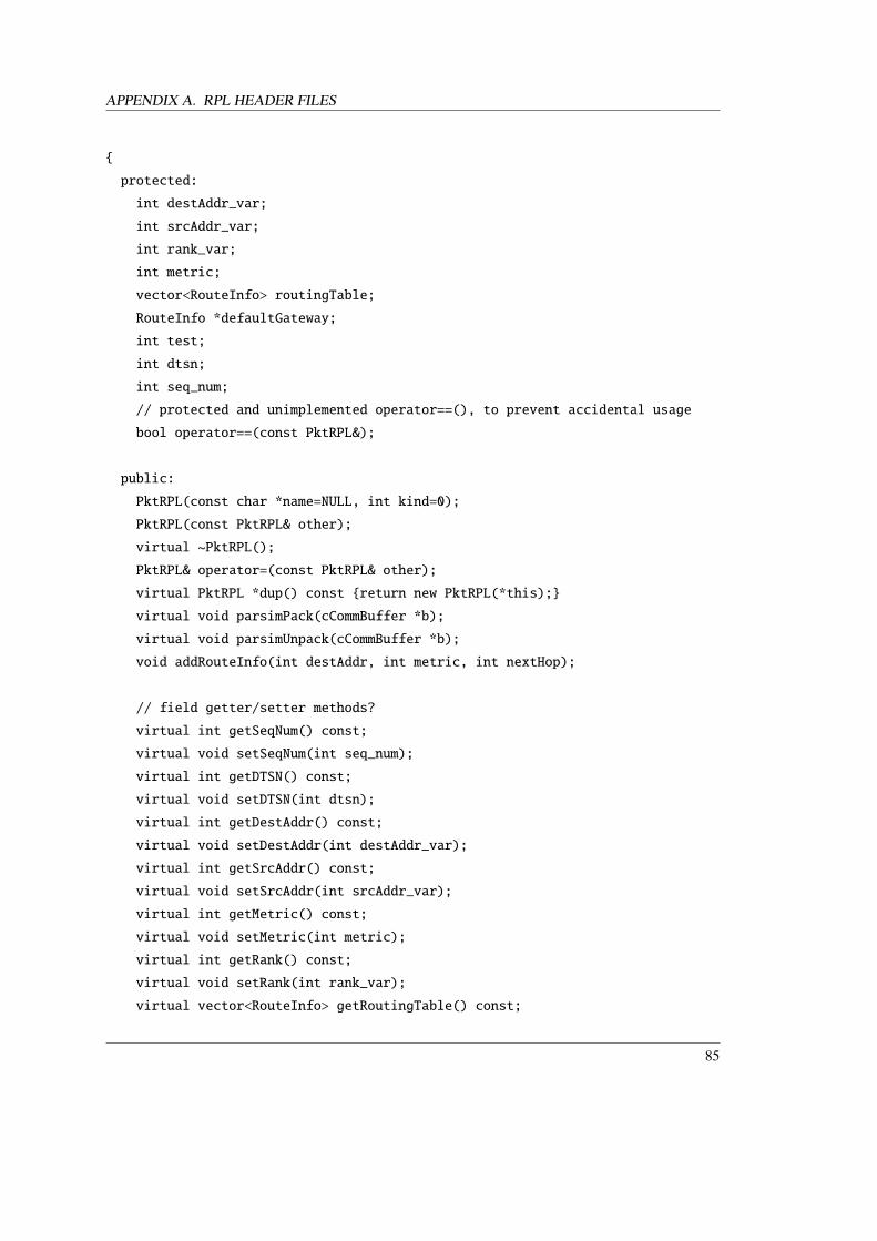
APPENDIX A. RPL HEADER FILES
{
protected:
int destAddr_var;
int srcAddr_var;
int rank_var;
int metric;
vector<RouteInfo> routingTable;
RouteInfo *defaultGateway;
int test;
int dtsn;
int seq_num;
// protected and unimplemented operator==(), to prevent accidental usage
bool operator==(const PktRPL&);
public:
PktRPL(const char *name=NULL, int kind=0);
PktRPL(const PktRPL& other);
virtual ~PktRPL();
PktRPL& operator=(const PktRPL& other);
virtual PktRPL *dup() const {return new PktRPL(*this);}
virtual void parsimPack(cCommBuffer *b);
virtual void parsimUnpack(cCommBuffer *b);
void addRouteInfo(int destAddr, int metric, int nextHop);
// field getter/setter methods?
virtual int getSeqNum() const;
virtual void setSeqNum(int seq_num);
virtual int getDTSN() const;
virtual void setDTSN(int dtsn);
virtual int getDestAddr() const;
virtual void setDestAddr(int destAddr_var);
virtual int getSrcAddr() const;
virtual void setSrcAddr(int srcAddr_var);
virtual int getMetric() const;
virtual void setMetric(int metric);
virtual int getRank() const;
virtual void setRank(int rank_var);
virtual vector<RouteInfo> getRoutingTable() const;
85

A.2. PKTRPL_M.H
virtual void setRoutingTable(vector<RouteInfo> routingTable);
virtual RouteInfo getDefaultGateway() const;
virtual void setDefaultGateway(RouteInfo *defaultGatway);
};
inline void doPacking(cCommBuffer *buffer, vector<RouteInfo> routingTable) {
vector<RouteInfo>::iterator routingTableItr;
for(routingTableItr = routingTable.begin(); routingTableItr != routingTable.end(); ++routingTableItr){
RouteInfo r = *routingTableItr;
buffer->pack(r.getDestAddr());
buffer->pack(r.getMetric());
buffer->pack(r.getNextHop());
}
}
inline void doPacking(cCommBuffer *buffer, RouteInfo *defaultGateway) {
buffer->pack((*defaultGateway).getDestAddr());
buffer->pack((*defaultGateway).getMetric());
buffer->pack((*defaultGateway).getNextHop());
}
inline void doUnpacking (cCommBuffer *buffer, vector<RouteInfo> routingTable) {
uint32 value;
vector<RouteInfo>::iterator routingTableItr;
for(routingTableItr = routingTable.begin(); routingTableItr != routingTable.end(); ++routingTableItr){
RouteInfo r = *routingTableItr;
buffer->unpack(value);
r.setDestAddr(value);
buffer->unpack(value);
r.setMetric(value);
buffer->unpack(value);
r.setNextHop(value);
}
}
inline void doUnpacking (cCommBuffer *buffer, RouteInfo *defaultGateway) {
uint32 value;
buffer->unpack(value);
86

APPENDIX A. RPL HEADER FILES
(*defaultGateway).setDestAddr(value);
buffer->unpack(value);
(*defaultGateway).setMetric(value);
buffer->unpack(value);
(*defaultGateway).setNextHop(value);
}
#endif // _PKTRPL_M_H_
A.3 Routing.h
// ***************************************************************************
// * file: Routing.h
// *
// * author: Simen Kurtzhals Hammerseth
// *
// * Routing.h file containing methods used while implementing Routing.
// *
// **************************************************************************/
#ifndef ROUTING_H_
#define ROUTING_H_
#include <BaseNetwLayer.h>
#include <PktRPL_m.h>
#include <ApplPkt_m.h>
#include <RouteInfo.h>
#include "BaseArp.h"
#include "NetwControlInfo.h"
#include "SimpleBattery.h"
class Routing : public BaseNetwLayer{
private:
vector<RouteInfo> routingTable;
RouteInfo* defaultGateway;
BaseArp* arp;
RouteInfo* parent;
87
A.3. ROUTING.H
public:
Routing();
virtual ~Routing();
void initialize();
void printRoutingTable();
void printDefaultGatway();
bool sendToNextHop(ApplPkt *pkt);
void sendToDefaultGatway(ApplPkt *pkt);
bool isRoot();
protected:
// The following redefined virtual function holds the algorithm.
//virtual void initialize();
virtual void handleMessage(cMessage *);
void handleNetMessage(cMessage *);
void handleRoutingTable(cMessage *);
};
#endif /* ROUTING_H_ */
88
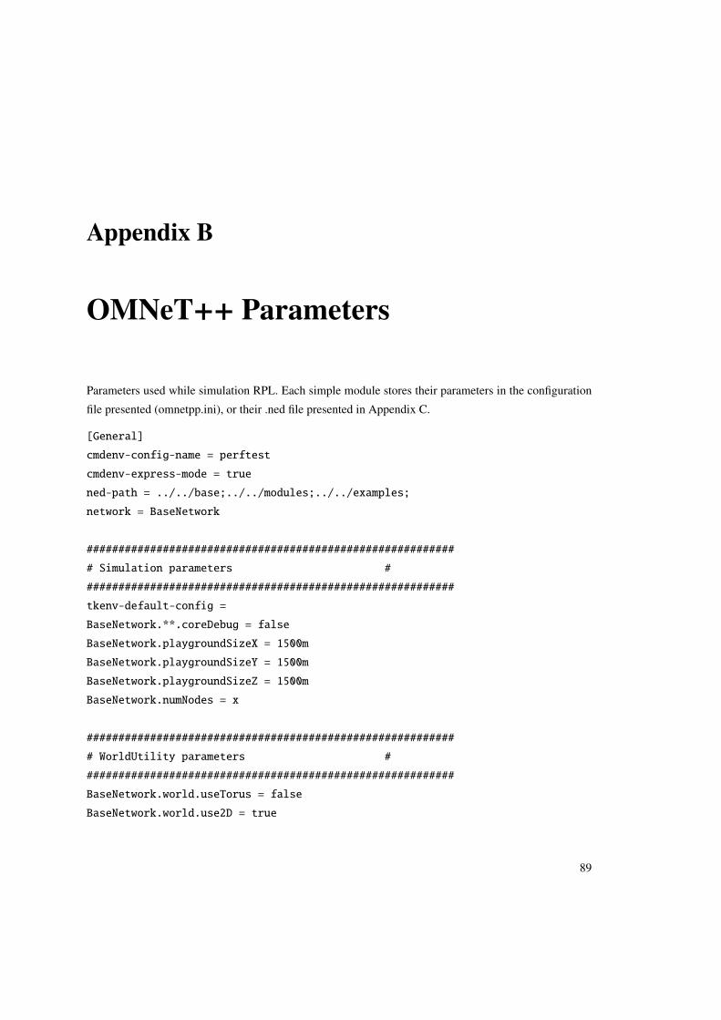
Appendix B
OMNeT++ Parameters
Parameters used while simulation RPL. Each simple module stores their parameters in the configuration
file presented (omnetpp.ini), or their .ned file presented in Appendix C.
[General]
cmdenv-config-name = perftest
cmdenv-express-mode = true
ned-path = ../../base;../../modules;../../examples;
network = BaseNetwork
##########################################################
# Simulation parameters #
##########################################################
tkenv-default-config =
BaseNetwork.**.coreDebug = false
BaseNetwork.playgroundSizeX = 1500m
BaseNetwork.playgroundSizeY = 1500m
BaseNetwork.playgroundSizeZ = 1500m
BaseNetwork.numNodes = x
##########################################################
# WorldUtility parameters #
##########################################################
BaseNetwork.world.useTorus = false
BaseNetwork.world.use2D = true
89
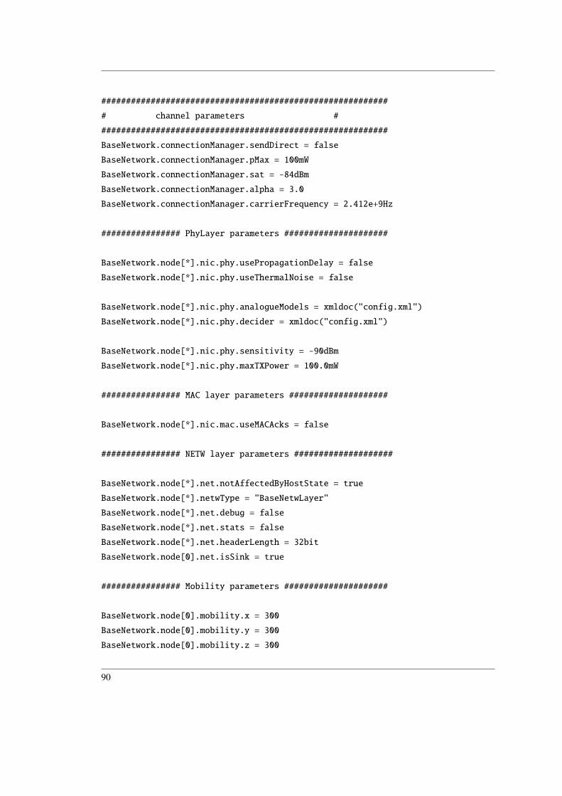
##########################################################
# channel parameters #
##########################################################
BaseNetwork.connectionManager.sendDirect = false
BaseNetwork.connectionManager.pMax = 100mW
BaseNetwork.connectionManager.sat = -84dBm
BaseNetwork.connectionManager.alpha = 3.0
BaseNetwork.connectionManager.carrierFrequency = 2.412e+9Hz
################ PhyLayer parameters #####################
BaseNetwork.node[*].nic.phy.usePropagationDelay = false
BaseNetwork.node[*].nic.phy.useThermalNoise = false
BaseNetwork.node[*].nic.phy.analogueModels = xmldoc("config.xml")
BaseNetwork.node[*].nic.phy.decider = xmldoc("config.xml")
BaseNetwork.node[*].nic.phy.sensitivity = -90dBm
BaseNetwork.node[*].nic.phy.maxTXPower = 100.0mW
################ MAC layer parameters ####################
BaseNetwork.node[*].nic.mac.useMACAcks = false
################ NETW layer parameters ####################
BaseNetwork.node[*].net.notAffectedByHostState = true
BaseNetwork.node[*].netwType = "BaseNetwLayer"
BaseNetwork.node[*].net.debug = false
BaseNetwork.node[*].net.stats = false
BaseNetwork.node[*].net.headerLength = 32bit
BaseNetwork.node[0].net.isSink = true
################ Mobility parameters #####################
BaseNetwork.node[0].mobility.x = 300
BaseNetwork.node[0].mobility.y = 300
BaseNetwork.node[0].mobility.z = 300
90

APPENDIX B. OMNET++ PARAMETERS
BaseNetwork.node[*].mobType = "ConstSpeedMobility"
BaseNetwork.node[*].mobility.debug = false
BaseNetwork.node[*].mobility.updateInterval = 0.1s
BaseNetwork.node[*].mobility.z = 0
BaseNetwork.node[*].mobility.speed = 0mps # 20mps
################ Application parameters #####################
BaseNetwork.node[*].applType = "TestApplication"
BaseNetwork.node[*].appl.debug = true
BaseNetwork.node[*].appl.flood = false
BaseNetwork.node[*].appl.stats = true
BaseNetwork.node[*].appl.payloadSize = 128 byte
BaseNetwork.node[*].appl.nbPackets = 10000
BaseNetwork.node[*].appl.trafficParam = 0.1
BaseNetwork.node[*].appl.trace = true
BaseNetwork.node[*].appl.convergeTime = 1s
BaseNetwork.node[0].appl.isSink = true
BaseNetwork.node[*].appl.numNodes = x
########### Battery parameters ###################
BaseNetwork.node[*].battery.debug = true
BaseNetwork.node[0].battery.capacity = 999999mAh
BaseNetwork.node[*].battery.nominal = 0.2525252525mAh #3000mA
BaseNetwork.node[*].battery.capacity = 0.2525252525mAh #3000mA
BaseNetwork.node[*].battery.voltage = 3.3V
BaseNetwork.node[*].battery.resolution = 0.1s
BaseNetwork.node[*].battery.publishDelta = 0.999#0.01
BaseNetwork.node[*].battery.publishTime = 0.999s#0.1s
BaseNetwork.node[*].battery.numDevices = 1
###########battery stats###########
BaseNetwork.node[*].batteryStats.debug = true
BaseNetwork.node[*].batteryStats.detail = true
BaseNetwork.node[*].batteryStats.timeSeries = false
91

################ Routing parameters #####################
BaseNetwork.node[0].routing.isSink = true
################ RPL parameters #####################
BaseNetwork.node[0].rpl.isSink = true
BaseNetwork.node[*].rpl.debug = true
BaseNetwork.node[*].rpl.hopCount = true
BaseNetwork.node[*].rpl.packetTime = (600/15000) * 1s #should be the maximum paket size divided by minimum bitrat
BaseNetwork.node[*].rpl.processingTime = 60s
92

Appendix C
Network Description File
The network description file contains the gates and parameters not specified in the configuration file
omnetpp.ini.
C.1 Nic802154_TI_CC2420.ned
//***************************************************************************
// * file: Nic802154_TI_CC2420.ned
// *
// * author: Jerome Rousselot, Marc Loebbers
// *
// * copyright: (C) 2008-2010 CSEM SA, Neuchatel, Switzerland.
// * (C) 2004 Telecommunication Networks Group (TKN) at
// * Technische Universitaet Berlin, Germany.
// *
// * This program is free software; you can redistribute it
// * and/or modify it under the terms of the GNU General Public
// * License as published by the Free Software Foundation; either
// * version 2 of the License, or (at your option) any later
// * version.
// * For further information see file COPYING
// * in the top level directory
// *
// * Funding: This work was partially financed by the European Commission under the
93

C.1. NIC802154_TI_CC2420.NED
// * Framework 6 IST Project "Wirelessly Accessible Sensor Populations"
// * (WASP) under contract IST-034963.
// **************************************************************************/
package org.mixim.modules.nic;
//
// This NIC implements a Texas Instruments CC 2420 802.15.4 network interface card
// using the CSMA protocol as specified in IEEE 802.15.4-2006.
//
//Note: To be able to use this Nic in your simulation you have to copy the file
//"Nic802154_TI_CC2420_Decider.xml" from "modules/nic/" to your simulation directory.
// @author Jerome Rousselot
//
module Nic802154_TI_CC2420 extends WirelessNicBattery
{
parameters:
macType = default("CSMA802154");
// power consumption from boards (at 3.3V)
sleepCurrent = 0.000021mA; // 0.021
rxCurrent = 18.8 mA;
decodingCurrentDelta = 0 mA;
txCurrent = 17.4 mA;
setupRxCurrent = 0.6391mA; // 0.002109 W
setupTxCurrent = 0.6845mA; // 0.002259 W
rxTxCurrent = 18.8 mA; // Upper bound
txRxCurrent = 18.8 mA; // idem
phy.decider = xmldoc("Nic802154_TI_CC2420_Decider.xml");
//publishRSSIAlways = false;
phy.headerLength = 48 bit; // ieee 802.15.4
phy.thermalNoise = -110 dBm;
// From TI CC1100 datasheet rev. C
phy.timeSleepToRX = 0.001792 s;
phy.timeSleepToTX = 0.001792 s;
phy.timeRXToTX = 0.000192 s;
phy.timeTXToRX = 0.000192 s;
94

APPENDIX C. NETWORK DESCRIPTION FILE
phy.timeRXToSleep = 0 s;
phy.timeTXToSleep = 0 s;
mac.rxSetupTime = 0.001792 s;
mac.txPower = default(1 mW);
}
95
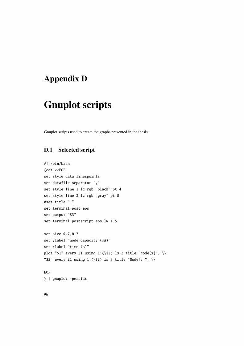
Appendix D
Gnuplot scripts
Gnuplot scripts used to create the graphs presented in the thesis.
D.1 Selected script
#! /bin/bash
(cat <<EOF
set style data linespoints
set datafile separator ","
set style line 1 lc rgb "black" pt 4
set style line 2 lc rgb "gray" pt 8
#set title "1"
set terminal post eps
set output "$3"
set terminal postscript eps lw 1.5
set size 0.7,0.7
set ylabel "node capacity (mA)"
set xlabel "time (s)"
plot "$1" every 21 using 1:(\$2) ls 2 title "Node[x]", \\
"$2" every 21 using 1:(\$2) ls 3 title "Node[y]", \\
EOF
) | gnuplot -persist
96

Appendix E
Java Programs
The three java programs used to filter output data form OMNeT++, and create network structures.
E.1 Gridder
import java.io.BufferedWriter;
import java.io.FileWriter;
import java.util.Random;
public class Gridder {
public static void main(String[] args) throws Exception {
FileWriter fstream = new FileWriter("test.txt");
BufferedWriter out = new BufferedWriter(fstream);
Random randomGen = new Random( 23422 );
int numNodes = 80;
int x = 500, y = 500, z = 0;
for(int i = 1; i<numNodes; i++){
x = 250 + randomGen.nextInt(750);
y = 250 + randomGen.nextInt(750);
out.write("BaseNetwork.node[" + i + "].mobility.x = "+ x + "\n");
out.write("BaseNetwork.node[" + i + "].mobility.y = "+ y + "\n");
out.write("BaseNetwork.node[" + i + "].mobility.z = "+ z + "\n\n");
97
E.2. BARCHART
}
}
out.close();
}
}
E.2 BarChart
import java.io.BufferedReader;
import java.io.BufferedWriter;
import java.io.DataInputStream;
import java.io.FileInputStream;
import java.io.FileWriter;
import java.io.InputStreamReader;
import java.util.ArrayList;
import java.util.Collections;
public class BarChart {
public static void main(String[] args) throws Exception {
FileWriter fout = new FileWriter("output");
BufferedWriter out = new BufferedWriter(fout);
FileInputStream fstream = new FileInputStream("input");
DataInputStream in = new DataInputStream(fstream);
BufferedReader br = new BufferedReader(new InputStreamReader(in));
String strLine;
ArrayList<Integer> liste = new ArrayList<Integer>();
while ((strLine = br.readLine()) != null) {
if(strLine.contains("died at simtime")){
int x = strLine.indexOf(":");
x+=2;
String time = strLine.substring(x);
98
APPENDIX E. JAVA PROGRAMS
int test = (int)Double.parseDouble(time);
if(test != 1){
liste.add(test);
}
}
}
Collections.sort(liste);
int deadNodes = 0;
int interval = 25;
int mul = 0, currMul = 0;
for (int i = 0; i < liste.size(); i++) {
currMul = liste.get(i)/interval;
if(mul == currMul){
deadNodes++;
mul = currMul;
}
else{
out.write(interval*(mul) + "-" + interval*(mul+1) + "," + deadNodes +
"\n");
deadNodes = 1;
mul = currMul;
}
//out.write(liste.get(i) + "," + y + "\n");
}
out.write(interval*(mul) + "-" + interval*(mul+1) + "," + deadNodes + "\n");
in.close();
out.close();
}
}
E.3 FilterOutput
import java.io.BufferedReader;
import java.io.BufferedWriter;
import java.io.DataInputStream;
import java.io.FileInputStream;
99

E.3. FILTEROUTPUT
import java.io.FileWriter;
import java.io.InputStreamReader;
import java.util.ArrayList;
public class FilterOutput {
public static void main(String[] args) throws Exception {
FileWriter fout = new FileWriter("output");
BufferedWriter out = new BufferedWriter(fout);
FileInputStream fstream = new FileInputStream("input");
DataInputStream in = new DataInputStream(fstream);
BufferedReader br = new BufferedReader(new InputStreamReader(in));
String strLine;
ArrayList<Double> liste = new ArrayList<Double>();
ArrayList<Double> liste2 = new ArrayList<Double>();
while ((strLine = br.readLine()) != null) {
if(strLine.contains(", Time")){
int x = strLine.indexOf("y:");
int y = strLine.indexOf(’,’);
x+=3;
String time = strLine.substring(x,y);
Double test = Double.parseDouble(time);
liste.add(test);
int z = strLine.indexOf("Time:");
z+=6;
String time2 = strLine.substring(z);
Double test2 = Double.parseDouble(time2);
liste2.add(test2);
}
}
//Collections.sort(liste);
for (int i = 0; i < liste.size(); i++) {
100
APPENDIX E. JAVA PROGRAMS
int y = i+1;
out.write(liste2.get(i) + "," + liste.get(i) + "\n");
}
in.close();
out.close();
}
}
101