Imperfect Common Knowledge, Price Stickiness, and Inflation Inertia

Porntawee Nantamanasikarn

University of Hawai’i at ManoaNovember 27, 2006

2

Introduction

The standard New Keynesian (NK) model does a poor job explaining observed inflation inertia (e.g. Mankiw, 2001)

Inflation response jumps immediately at the time of monetary shocks, because price, but not inflation, is sticky, and the representative agent is purely forward looking

3

Other Studies’ Proposed Solutions

Backward looking behavior Fuhrer and Moore (1995), Gali and Gertler (1999)

Limited or bounded rationality Roberts (1997), Ball (2000)

Automatic indexation to past inflation Yun (1996), Christiano et al. (2005)

4

Other Studies’ Proposed Solutions

Information stickiness Mankiw and Reis (2002, 2003)

Implementation lags Cochrane (1998), Bernanke and Woodford (1997)

Habit persistence Fuhrer (2000), Smets and Wouters (2003)

5

The Noisy Information (NI) Model

Woodford (2003) assumes monopolistic competitive market in Lucas’s (1973) island model to generate inflation inertia

Firms have heterogeneous subjective perceptions of current conditions (imperfect common knowledge)

Inflation responds sluggishly to monetary shock because higher-order expectations are slow to adjust

6

The NI Model’s Problems

Prices are fully flexible Implication: credible future policy change does not

affect current decisions

Can generate inflation persistence only if the monetary shock is persistent Implication: inflation inertia is the result of external

drivers, not internal propagation mechanism

7

The NI Model’s Problems

Firms have (noisy) information only on exogenous nominal spending, not on the endogenous aggregate price level

Agents’ perceptions are not affected by others’ current decisions

8

Research Objective

Develop models that credible future policy can affect current decisions can generate inflation inertia, even if monetary

shock is not very persistent others’ decisions simultaneously affect perceptions

How: assume imperfect CK and price stickiness

Challenge: the infinite regress problem

9

The Infinite Regress Problem

Dating back to Pigou (1929), Muth (1960)

The recursive representation of the system requires infinite number of state variables

When agents must forecast the forecasts of others (which is unobserved), it is necessary for them to keep track of infinite history of observable variables

10

The Infinite Regress Problem

Some proposed “solutions”: Townsend (1983), Lucas (1975)

The NI model avoids this problem because there is no feedback from pricing decisions to the source of signals

I propose two alternative models for how expectations are formed: The Rational Believer (RB) Model The Limited Depth of Reasoning (LDR) Model

11

Summary of Model Comparisons

Lucas (1973)

NK NI RB/

LDR

Perfectly competitive market? yes no no no

Flexible price? yes no yes no

Perfect (common) information? no yes no no

Infinite regress problem? no no no yes

12

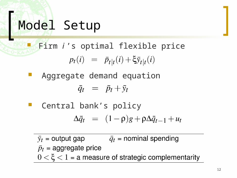
Firm i ’s optimal flexible price

Aggregate demand equation

Central bank’s policy

Model Setup

13

Adding Price Stickiness

Firms have a constant probability of (1-to adjust price in each period (Calvo 1983)

If able to adjust price, a forward looking firm will set the new price, according to

The aggregate price is

14

Notations

15

Higher-Order Expectations

16

The Heterogeneous Information Phillips Curve

17

Firms’ Perceived Law of Motion

18

Firms’ Signal Equation

Each firm receives idiosyncratic signal of the state variables according to

is mean-zero Gaussian white noise error terms, distributed independently both of the history of fundamental disturbance and of the observation errors of all other agents

19

The Kalman Filter Updating Algorithm

Firms form minimum MSE estimates of the state variables, according to

where K is a matrix of Kalman gain

The equilibrium objects are L,M,N, which result in a fixed point of mapping from the perceived law of motion to the actual one when firms’ updating algorithm is the above equation

20

The Rational Believer Model

In a special case that A,B,D are known a priori, and C=0 and Q2=0, the equilibrium matrices L,M,N are exactly identified. Otherwise, there are more unknown variables than the number of equilibrium conditions

C=0 means that firms (mistakenly) believe that the actual aggregate price and nominal spending do not depend on their higher-order expectations

Q2=0 means that firms receive signals on the actual price and nominal spending, but not on their higher-order expectations

21

The Rational Believer Model

The RB model assumes that firms believe and know that others also believe the economy evolves according to the full-info NK model

But they are unaware that their own decisions affect the aggregate outcome

Misperception persists because firms’ information set consists of only a history of contaminated signals, which cannot be used to prove that the NK model is actually wrong

22

The Limited Depth of Reasoning Model

Firms are aware that their own decisions affect the aggregate outcome

But they can form expectations of others’ forecasts only for a finite (k) number of iterations (see the price eq.)

This is supported by the experimental evidence in Nagel (1995)

23

The Limited Depth of Reasoning Model

Suppose that k=3, that is, firms assume that the 4th order expectation is the same as the 3rd

The state vector is

Limited depth of reasoning means

24

The Impulse Response Functions

Assume that firms receive signals on contemporaneous nominal spending and aggregate price level (Q2=0)

Using the baseline parameter values from Woodford (2003)

25

Baseline Inflation Response

0 5 10 150

0.1

0.2

0.3

0.4

0.5

0.6

0.7

NKNIRBLDR

26

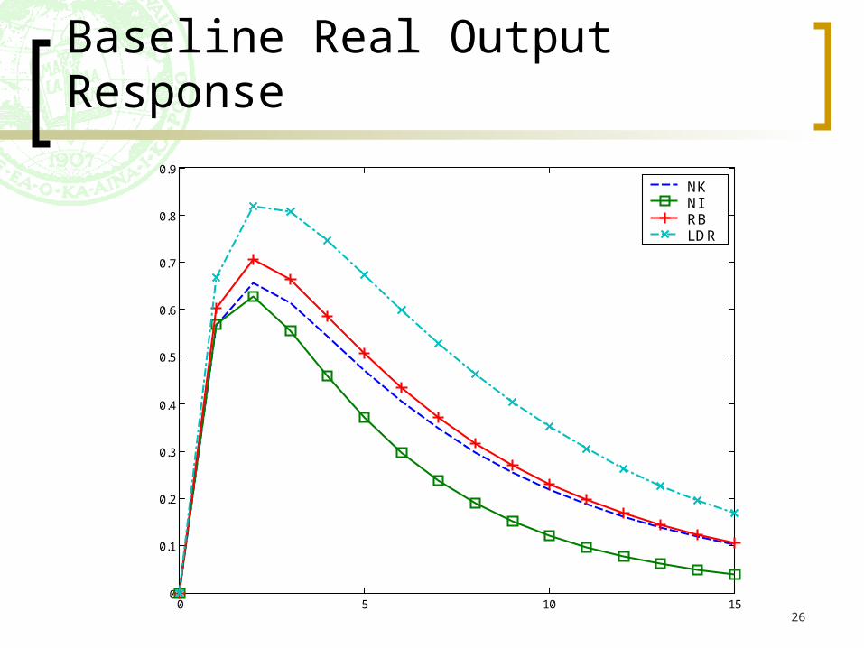
Baseline Real Output Response

0 5 10 150

0.1

0.2

0.3

0.4

0.5

0.6

0.7

0.8

0.9

NKNIRBLDR

27

Inflation Response of the LDR Model, for varying k

0 5 10 150

0.1

0.2

0.3

0.4

0.5

0.6

0.7

k=1k=3k=6k=10NI

28

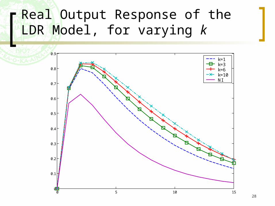
Real Output Response of the LDR Model, for varying k

0 5 10 150

0.1

0.2

0.3

0.4

0.5

0.6

0.7

0.8

0.9

k=1k=3k=6k=10NI

29

Inflation Response of the NI Model, for varying

0 5 10 150

0.1

0.2

0.3

0.4

0.5

0.6

0.7=0=0.3=0.6=0.9LDR (=0.3)

30

Real Output Response of the NI Models,

for varying

0 5 10 15-0.1

0

0.1

0.2

0.3

0.4

0.5

0.6

0.7

0.8

0.9=0=0.3=0.6=0.9LDR (=0.3)

31

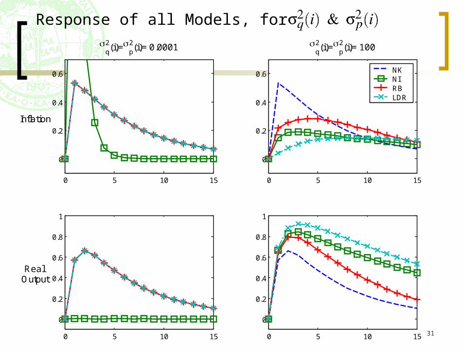
Response of all Models, for varying

0 5 10 15

0

0.2

0.4

0.6

2q(i)=2

p(i)= 0.0001

Inflation

0 5 10 15

0

0.2

0.4

0.6

0.8

1

Real Output

0 5 10 15

0

0.2

0.4

0.6

2q(i)=2

p(i)= 100

NKNIRBLDR

0 5 10 15

0

0.2

0.4

0.6

0.8

1

32

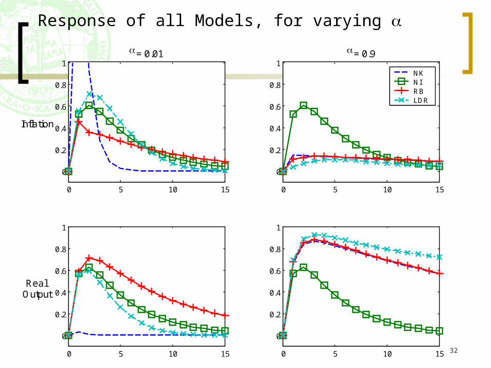
Response of all Models, for varying

0 5 10 15

0

0.2

0.4

0.6

0.8

1

= 0.01

Inflation

0 5 10 15

0

0.2

0.4

0.6

0.8

1

Real Output

0 5 10 15

0

0.2

0.4

0.6

0.8

1

= 0.9

NKNIRBLDR

0 5 10 15

0

0.2

0.4

0.6

0.8

1

33

Conclusion

The models can generate inflation inertia, even when monetary shocks are not persistent, esp. the LDR model

But it is necessary that we make assumptions about how expectations are formed to “solve” the infinite regress problem

Extension: endogenize price stickiness