Impact of Foot-and -Mouth Disease Management...

Amy D. Hagerman

Bruce A. McCarl

Tim Carpenter

Josh O'Brien

10/30/2009

Impact of Foot-and-Mouth

Disease Management

Alternatives in the California

Dairy Industry

Impact of Foot-and-Mouth Disease Management

Alternatives in the California Dairy Industry

October 30, 2009

Amy D. Hagerman

Research Associate

Department of Agricultural Economics

Texas A&M University.

Bruce A. McCarl

Distinguished Professor and Regents Professor

Department of Agricultural Economics

Texas A&M University.

Tim Carpenter

Professor of Epidemiology

Co-Director of the Center for Animal Disease Modeling and Surveillance (CADMS)

University of California, Davis

Josh O’Brien

Biologist and Programmer

Center for Animal Disease Modeling and Surveillance (CADMS)

Funded by the Department of Homeland Security funded National Center of Excellence for the

study of Foreign Animal and Zoonotic Disease Defense headquartered at Texas A&M University.

Table of Contents Page

1. INTRODUCTION .............................................................................................................. 1

2. BACKGROUND ON CALIFORNIA LIVESTOCK AGRICULTURE .............................................. 1

3. STUDY DESIGN ............................................................................................................... 2

3.1. SCENARIOS.......................................................................................................................... 2

4. DISEASE IMPACT CATEGORIZATIONS .............................................................................. 4

4.1. DIRECT LOSSES .................................................................................................................... 4

1.1.1. Lost Animals and Changes in Animal Value ................................................................ 4

1.1.2. Costs of Disease Management ................................................................................... 5

1.1.3. Trade Losses ................................................................................................................ 6

4.2. SECONDARY LOSSES .............................................................................................................. 6

1.1.4. Related Industries ....................................................................................................... 7

1.1.5. Local Economies .......................................................................................................... 8

1.1.6. Environmental Impacts ............................................................................................... 9

1.1.7. Meat Demand ........................................................................................................... 10

4.3. COST ASSUMPTIONS SPECIFIC TO THIS STUDY .......................................................................... 10

4.4. HERD DEMOGRAPHICS ........................................................................................................ 13

5. EPIDEMIC MODEL RESULTS ........................................................................................... 15

5.1. ANIMALS SLAUGHTERED FOR DISEASE CONTROL ....................................................................... 15

5.2. HERDS PLACED UNDER MOVEMENT RESTRICTIONS ................................................................... 16

5.3. ANIMALS SLAUGHTERED FOR WELFARE PURPOSES .................................................................... 18

6. ECONOMIC MODEL RESULTS ........................................................................................ 19

6.1. NATIONAL AGRICULTURAL ECONOMIC SURPLUS IMPACTS UNDER ALTERNATIVE DELAYS IN DETECTION

AND VACCINATION ......................................................................................................................... 20

6.2. RISK AVERSION ANALYSIS .................................................................................................... 25

6.3. THE COST OF AN ADDITIONAL HOUR DELAY IN DETECTION ......................................................... 27

6.4. PRICE IMPACTS .................................................................................................................. 28

1.1.8. Price Impacts for Live Animals .................................................................................. 28

1.1.9. Price Impacts for Meat and Livestock Products Excluding Dairy .............................. 30

1.1.10. Price Impacts for Dairy Products .......................................................................... 31

1.11. Price Impacts for Feed Grains ............................................................................... 32

1.1.12. Summary of Price Changes ................................................................................... 33

6.5. REGIONAL LIVESTOCK PRODUCER SURPLUS IMPACTS ................................................................. 33

1.1.13. Total US Livestock Producer Surplus Changes ...................................................... 34

1.1.14. Pacific Southwest (PSW) ....................................................................................... 35

1.1.15. Dairy Producing Regions ....................................................................................... 35

1.1.16. Other Livestock and Grain Production Regions .................................................... 36

6.6. TRADE IMPACT ANALYSIS ..................................................................................................... 39

7. CONCLUSIONS AND IMPLICATIONS ............................................................................... 40

8. REFERENCES ................................................................................................................. 42

9. APPENDIX: INTEGRATED EPIDEMIC/ECONOMIC MODELING .......................................... 45

9.1. GENERAL FRAMEWORK ....................................................................................................... 45

9.1.1. Defining Scenarios .................................................................................................... 45

9.1.2. Epidemic Modeling ................................................................................................... 46

9.1.2.1. The Davis Animal Disease Simulation (DADS) Model ....................................... 47

9.1.3. Economic Modeling .................................................................................................. 47

9.1.3.1. FASOM............................................................................................................... 48

List of Tables Page

Table 1. Epidemic Model Scenario Definitions ............................................................................... 3

Table 2. Market Price Assumptions .............................................................................................. 13

Table 3. Herd Definitions from DADS Model ................................................................................ 14

Table 4. Inventories of Animals in Susceptible Region When Moved to ASM ............................. 14

Table 5. Summary Statistics for Disease Control Slaughter .......................................................... 15

Table 6. Summary Statistics for Herds Quarantined .................................................................... 17

Table 7. Summary Statistics for Head in Danger of Slaughter for Welfare Purposes .................. 18

Table 8. Summary Statistics for National Loss in Total Agricultural Surplus-No Vaccination

(Millions of 2004$) ........................................................................................................................ 21

Table 9. Summary Statistics for National Loss in Total Agricultural Surplus -- 10 Km Ring

Vaccination (Millions of 2004$) .................................................................................................... 21


Vaccination (Millions of 2004$) .................................................................................................... 21

Table 11. Mean Prices of Live Cattle Under Alternative Days of Detection ................................ 29

Table 12. Mean Prices of Live Hogs and Sheep Under Alternative Days of Detection ................. 29

Table 13. Mean Prices of Eggs and Live Poultry Under Alternative Days of Detection ................ 30

Table 14. Mean Prices of Beef, Pork and Poultry Under Alternative Days to Detection ............. 31

Table 15. Mean Price of Wool Under Alternative Days to Detection ........................................... 31

Table 16. Mean Price of Dairy Products Under Alternative Days to Detection ............................ 32

Table 17. Mean Price of Feed Grains Under Alternative Days to Detection ................................ 32

Table 18. Summary Statistics for Total Livestock Producers' Surplus Changes Relative to the

Base Scenario ................................................................................................................................ 34

Table 19. Summary Statistics for California (Pacific Southwest) Livestock Producers' Surplus

Changes Relative to the Base Scenario ......................................................................................... 35

Table 20. Summary Statistics for Other Dairy Producing Regions Livestock Producers' Surplus

Changes Relative to the Base Scenario ......................................................................................... 36

Table 21. Summary Statistics for Great Plains Region Livestock Producers' Surplus Changes

Relative to the Base Scenario ....................................................................................................... 37

Page

Table 22. Summary Statistics for Southwest Region Livestock Producers' Surplus Changes


Table 23. Summary Statistics for Corn Belt Region Livestock Producers' Surplus Changes


Table 24. Summary Statistics for South Central Region Livestock Producers' Surplus Changes


Table 25. Summary Statistics for Southeast Region Livestock Producers' Surplus Changes


List of Figures Page

Figure 1. Interrelationship of Livestock Sector (Pritchett, Thilmany and Johnson) ....................... 7

Figure 2. Spread of Disease Control Slaughter Distribution ......................................................... 16

Figure 3. Spread of Herds Quarantined Distribution .................................................................... 17

Figure 4. Spread of Head in Danger of Welfare Slaughter............................................................ 19

Figure 5. ASM Sub-Regional Breakdown of California .................................................................. 20

Figure 6. Box Plot of National Agricultural Surplus Loss Spread -- No Vaccination ...................... 22

Figure 7. Box Plot of National Agricultural Surplus Loss Spread -- 10 Km Ring Vaccination ........ 23

Figure 8. Box Plot of National Agricultural Surplus Loss Spread -- 20 Km Ring Vaccination ........ 24

Figure 9. Box Plot of National Agricultural Surplus Loss Spread Under Alternative Vaccination . 25

Figure 10. SERF Diagram Under Alternative Scenarios ................................................................. 26

Figure 11. Box Plot of Cost per Hour of Delay between 21 and 22 Days ..................................... 28

Figure 12. ASM Regions and Sub-regions ..................................................................................... 33

Figure 13. Basic FASOM Modeling Structure and Disease Shock Imposition ............................ 50

Figure 14. International Market Regions in ASM ........................................................................ 51

Executive Summary

This report is a case study of FMD strategy analysis in the context of the California central valley

dairy industry. California is particularly susceptible to animal disease outbreaks due to the

importance of agricultural production to the state's economy. California's value of agricultural

products was valued at $33 billion in 2007. The study focuses particularly on simulating an

outbreak in the dairy industry, a $6.9 billion sales industry in a state that produces 22% of the

nation's milk supply. Control strategies considered are alternative detection and vaccination

approaches.

Results indicate that earlier detection is always a best response strategy in terms of reducing

epidemic size, disease control cost, and national welfare loss. They also show vaccination

increases slaughter, as would be expected given US "vaccinate to die" policy. However,

vaccination reduces the number of head placed under movement restrictions. Implications of

this extend beyond the size of the outbreak. By keeping the quarantine zone as small as is

reasonable, it lessens the welfare slaughter potential. Vaccination does come at a higher

economic national surplus loss and disease control cost. Examining the distribution of losses

and accounting for risk attitude on the part of policy makers, I find that vaccination is a risk

reducing strategy. This implies the undesirable tail of the distribution of losses is reduced such

that there is less chance of an extremely bad outcome.

Producers suffer the most from the outbreak, but simulation evidence suggests that producers

in some non-infected regions gain from the outbreak. In dairy production regions outside of

California, producers gain from the outbreak. However, for regions with hog production (an

FMD susceptible species and therefore subject to trade restrictions) producers have losses due

to international trade restrictions.

1

1. Introduction

California is the number one dairy producing state in the U.S. with 1.87 million head of cows

producing $6.5 billion worth of milk and other dairy products in 2007 (USDA-NASS, 2008). Foot

and mouth disease (FMD) is a large potential threat to the health and economic productivity of

this industry. Herein a joint epidemic-economic study examining the consequences of an FMD

outbreak in this industry was carried out to examine the effect of a number of management

alternatives. The focus of this study was the Central Valley in Northern California. The exact

index infection point of the outbreak will be chosen at random to avoid security sensitivities.

This study is a part of the larger research and development effort of the National Center for

Foreign Animal and Zoonotic Disease Defense (FAZD) to develop and employ a set of integrated

economic and epidemic models and databases as a part of an overall decision support system.

The goal of this research is to provide a quantitative approach for analyzing the impact of

alternative strategies for prevention, intervention and recovery and provide the resultant

information to decision makers in an attempt to assist them in planning and responding to

outbreaks of foreign animal and zoonotic disease. The models that have been used here are the

Davis Animal Disease Simulation (DADS) model and the Agricultural Sector Model (ASM)

component of the Forest and Agricultural Sector Optimization Model (FASOM).

Prior studies within the FAZD have looked at the impact of FMD on the Texas High Plains

concentrated beef cattle feeding sector and work at CADMS has looked the economics of FMD

in the Central Valley of California. This study will expand prior work and utilize the DADS-ASM

link to further examine the impact of FMD and management alternatives in the California dairy

sector.

2. Background on California Livestock Agriculture

According to the 2007 Census of Agriculture, California was ranked as having the highest total

value of agricultural products sold in the US at $33 billion. The majority of this comes from

crops, nursery and greenhouse products; however, the production of livestock, poultry and

their associated products was a $10.9 billion industry (NASS-USDA, 2008). California is ranked

second only to Texas in terms of livestock value.

In California milk and other dairy products from cows are the highest value livestock

commodity group at $6.9 billion in value of sales; this represents 22% of the nation's milk

supply. This is followed by cattle and calves ($2.5 billion), and poultry and eggs ($1.5 billion)

2

(USDA-NASS, 2009). Swine, sheep, goats and other animals make up a relatively small portion of

the state's value of livestock. In terms of numbers of animals, poultry were the largest animal

category, but cattle and calves represented 5.5 billion animals (USDA-NASS, 2009).

California is ranked first in dairy production in the US followed by Wisconsin, New York, Idaho

and Pennsylvania (Dapper et al.). It is hypothesized that these other regions could potentially

gain from a major animal disease outbreak in California due to slashed milk supplies and

consequently increased milk prices. In 2008, total annual milk production in California

surpassed 40 billion pounds (Francesconi et al.). This was a record breaking year, and dairy

cooperatives and other processing plants initiated base caps for producers. There are 34 milk

producing counties in the state, but almost 70% is produced in Tulare, Merced, Stanislaus, Kings

and Kern counties (Dapper et al.). This area is the focus of the study presented here,

particularly Tulare county.

The utilization of milk has been primarily for butter and nonfat dry milk powder (34% of

production) and cheese production (43% of production) where the primary cheeses produced

are Mozzarella, Cheddar and Jack (Dapper et al.). The leading counties in dairy manufacturing

capacity are Merced, Tulare, Madera, Humboldt and Yolo accounting for a total of 86% of

manufacturing capacity among them (Dapper et al.). There were 117 plants in California in 2008

(Dapper et al.), creating the potential for a bottleneck for remaining facilities if a large number

of these facilities are under movement restrictions. If the manufacturing facility is located in the

county infected by disease, it will also be under movement restrictions halting the movement

of products outside the movement restriction zone. Furthermore, there is a question as yet

unanswered of whether manufacturing facilities would allow milk from premises under

surveillance for the disease from entering their operation without stringent testing and cleaning

of trucks.

3. Study Design

3.1. Scenarios

The hypothetical FMD outbreak was initiated in a dairy herd by contact with a feral hog, and

subsequently spread through California's population of domesticated livestock. The epidemic

was simulated using the DADS model. Resulting data on the losses from the epidemic were run

through the ASM component of the FASOM model to gain perspective on the economic

consequences of the disease, including both the direct disease mitigation costs and other

economic consequences. Specific disease mitigation issues considered here were:

3

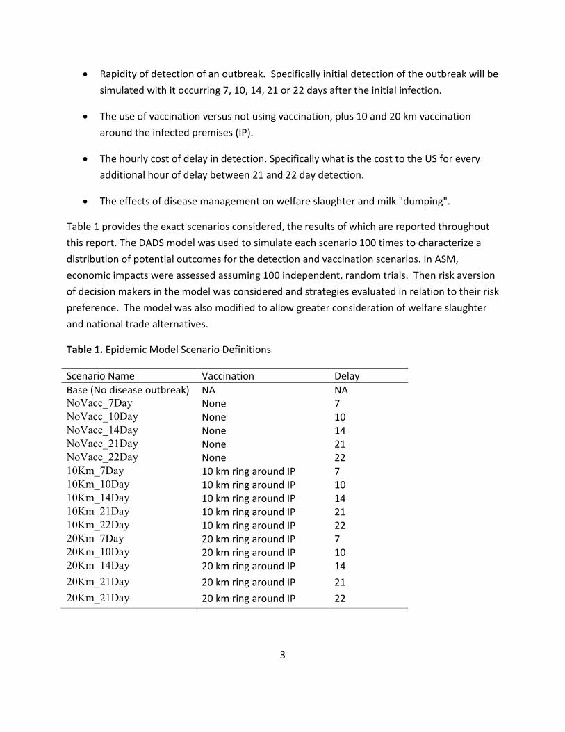
• Rapidity of detection of an outbreak. Specifically initial detection of the outbreak will be

simulated with it occurring 7, 10, 14, 21 or 22 days after the initial infection.

• The use of vaccination versus not using vaccination, plus 10 and 20 km vaccination

around the infected premises (IP).

• The hourly cost of delay in detection. Specifically what is the cost to the US for every

additional hour of delay between 21 and 22 day detection.

• The effects of disease management on welfare slaughter and milk "dumping".

Table 1 provides the exact scenarios considered, the results of which are reported throughout

this report. The DADS model was used to simulate each scenario 100 times to characterize a

distribution of potential outcomes for the detection and vaccination scenarios. In ASM,

economic impacts were assessed assuming 100 independent, random trials. Then risk aversion

of decision makers in the model was considered and strategies evaluated in relation to their risk

preference. The model was also modified to allow greater consideration of welfare slaughter

and national trade alternatives.

Table 1. Epidemic Model Scenario Definitions

Scenario Name Vaccination Delay

Base (No disease outbreak) NA NA

NoVacc_7Day None 7

NoVacc_10Day None 10




10Km_7Day 10 km ring around IP 7










4

4. Disease Impact Categorizations

Economic impacts can be divided into two categories: direct and secondary. Most studies

examining livestock disease have focused on direct impacts of the disease. Due to the highly

integrated nature of the modern economy, consequences of agricultural contamination at any

given point along the supply chain could be manifested in other sectors of the economy as well.

For example in the recent foot FMD outbreak in the UK, the largest category of losses came

from tourism. Such losses are termed secondary losses.

The losses that should be examined in any given epidemic-economic study will vary depending

on the type of disease, species of animals impacted and the importance of those species to the

economy, as well as regional and international animal disease policies.

4.1. Direct Losses

Direct losses accumulate to the livestock sector as a direct consequence of an animal disease

attack. This category of losses has received the most attention because they are typically easily

quantified, particularly for the supply side. Direct losses are also of interest in establishing the

cost of a particular response policy from a governing agency viewpoint.

1.1.1. Lost Animals and Changes in Animal Value

The most obvious direct loss results from animals or herds that are removed from the supply

chain due to the disease. This may arise from massive preventative slaughter, as in the case of

FMD, or death due to the disease itself, such as with BSE. It also captures increased culling and

abortion in young animals for production operations, as would be the case with Rift Valley

Fever.

The value of animals lost can be calculated using a schedule of market values based on pre-

disease market conditions. This is often the method used in studies for calculating indemnity

payments to producers from preventative slaughter. There are two issues with using this

method. First, it does not recognize the role of livestock as a capital asset (Thompson et al.). In

particular for purebred animal producers, the value of an animal represents an investment in

genetic improvements that may not be accounted for in a per pound cash market value as it

would for a commercial animal. Second, producers who have animals not infected but

expecting to absorb the full revenue loss from a negative price change may be tempted to claim

their herd has been in direct contact with infected herds in order to collect a higher price per

unit. It is suspected that the payout schedule was set too high in the 2001 FMD outbreak,

leading to slaughter levels greater than necessary for disease control (Anderson, 2002).

5

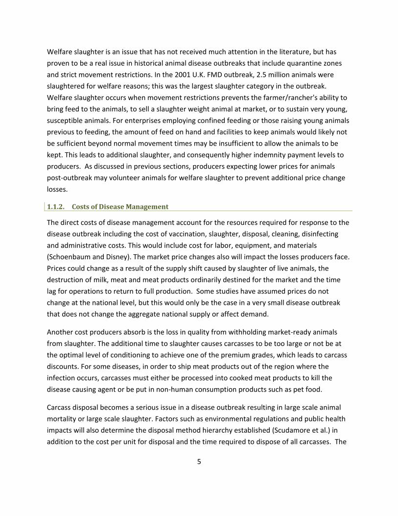
Welfare slaughter is an issue that has not received much attention in the literature, but has

proven to be a real issue in historical animal disease outbreaks that include quarantine zones

and strict movement restrictions. In the 2001 U.K. FMD outbreak, 2.5 million animals were

slaughtered for welfare reasons; this was the largest slaughter category in the outbreak.

Welfare slaughter occurs when movement restrictions prevents the farmer/rancher's ability to

bring feed to the animals, to sell a slaughter weight animal at market, or to sustain very young,

susceptible animals. For enterprises employing confined feeding or those raising young animals

previous to feeding, the amount of feed on hand and facilities to keep animals would likely not

be sufficient beyond normal movement times may be insufficient to allow the animals to be

kept. This leads to additional slaughter, and consequently higher indemnity payment levels to

producers. As discussed in previous sections, producers expecting lower prices for animals

post-outbreak may volunteer animals for welfare slaughter to prevent additional price change

losses.

1.1.2. Costs of Disease Management

The direct costs of disease management account for the resources required for response to the

disease outbreak including the cost of vaccination, slaughter, disposal, cleaning, disinfecting

and administrative costs. This would include cost for labor, equipment, and materials

(Schoenbaum and Disney). The market price changes also will impact the losses producers face.

Prices could change as a result of the supply shift caused by slaughter of live animals, the

destruction of milk, meat and meat products ordinarily destined for the market and the time

lag for operations to return to full production. Some studies have assumed prices do not

change at the national level, but this would only be the case in a very small disease outbreak

that does not change the aggregate national supply or affect demand.

Another cost producers absorb is the loss in quality from withholding market-ready animals

from slaughter. The additional time to slaughter causes carcasses to be too large or not be at

the optimal level of conditioning to achieve one of the premium grades, which leads to carcass

discounts. For some diseases, in order to ship meat products out of the region where the

infection occurs, carcasses must either be processed into cooked meat products to kill the

disease causing agent or be put in non-human consumption products such as pet food.

Carcass disposal becomes a serious issue in a disease outbreak resulting in large scale animal

mortality or large scale slaughter. Factors such as environmental regulations and public health

impacts will also determine the disposal method hierarchy established (Scudamore et al.) in

addition to the cost per unit for disposal and the time required to dispose of all carcasses. The

6

type of control strategy employed can also affect the carcass disposal method chosen since it

will, hopefully, reduce the number of dead animals (Jin, Huang and McCarl).

1.1.3. Trade Losses

Animal disease often has significant impacts on international trade. Outbreaks in the last

decade have increased the volatility in international meat markets through their effects on

consumer preferences, trade patterns, and reduced aggregate supply (Morgan and Prakash).

Upon confirmation of an animal disease outbreak, restrictions are often placed on where

livestock and meat products can be exported as well as what products are shipped. The extent

of these damages will vary by disease and country, but in general countries experiencing an

animal disease outbreak will experience immediate restricted international trade due to

domestic supply changes and world demand shifts until the infected country is shown to be

disease free for a pre-determined amount of time. Domestic market impacts may be partially

offset by imports (Thompson et al.).

If the disease is not carried in the meat, localized cuts in production will reduce the livestock

and meat products available for export. In addition, movement restrictions in the country will

prevent normal supplies from reaching the market and export restriction shift meat normally

shipped overseas to domestic supply (Thompson et al.).

If the disease is carried in the meat, it either must be cooked to destroy the organism or it must

be removed from the meat supply chain. Upon confirmation of BSE in the US in 2003, more

than 50 countries either completely stopped beef exports from the US or severely restricted

them resulting in beef exports at only 20% of the previous year's levels (Hu and Jin).

Even in the case of diseases that can be transferred to humans through the meat, markets have

historically been found to recover within two years; however, the nation that experienced the

outbreak may take longer to recover their share of the world market (Morgan and Prakash). At

particular risk are developing countries.

4.2. Secondary Losses

Secondary losses are less easily quantified, but ignoring them in a study can lead to severe

under-estimation of the total cost of the outbreak. These studies are often done separately

from the integrated epidemic-economic model analysis; however, they should ideally be

included in the integrated model as much as possible. In some cases, such as environmental

costs, the estimation may have to be done separately.

7

1.1.4. Related Industries

Disease outbreaks can have effects that extend well beyond the meat production chain

(Pritchett, Thilmany and Johnson). While industries directly in the meat production chain will

typically experience the greater loss and have consequently been the focus of disease outbreak

economics literature, little work has been done to ascertain the impact on service industries

linked to the meat industry. Figure 1, adapted from Pritchett, Thilmany and Johnson provides a

general idea of how interrelated these markets are. A good example is the feed industry. In

countries with large concentrated animal feeding operations, such as the US, a significant

source of demand for feed grains is represented by livestock demand. Disease outbreaks

leading to large scale animal mortality will reduce the domestic demand for feed grains. In

addition, movement restrictions in the quarantine zone will restrict not only the transport of

livestock but the transport of feed grain supply trucks/unit trains coming into or out of the

region. These disruptions and demand shifts will be reflected in the price of feed grains. Other

industries that would be impacted by a disease outbreak are transportation, veterinary service

and supply industries, and rendering services (Pritchett, Thilmany and Johnson).

Figure 1. Interrelationship of Livestock Sector (Pritchett, Thilmany and Johnson)

8

1.1.5. Local Economies

Disease outbreaks will have the greatest monetary impact on the area where the outbreak

occurs. Local producers whose premises are depopulated must wait to rebuild their operation,

removing the money that would have been spent on feed, supplies, and livestock related

services at local businesses. Movement restrictions divert commercial and tourist traffic coming

through the region, removing income to local businesses like gas stations, hotels and

restaurants. Businesses may choose to shut down or livestock operations may opt not to

repopulate, decreasing the number of jobs available to local residents. Alternatively, the

process of controlling the disease may provide some increased local employment but this

would be short term only.

In the 2001, UK FMD outbreak 44% of the confirmed cases occurred in the county of Cumbria

(Bennett et al.). Farmers and businesses in the county were surveyed after the outbreak to

ascertain their losses. Although 63% of farmers in the county said they would continue farming,

only 46% planned to build back up to their previous level of operation. There was an estimated

direct employment loss of 600 full-time jobs and an indirect employment loss of 900 jobs

(Bennett et al.).

In the entire north east region of the UK, 52% of businesses reported negative impacts but

these impacts were spread across various sectors (Phillipson et al.). Relatively low impacts were

felt by construction, education, health care, and personal services and moderately impacted

firms were retail, transportation, business services and manufacturing. Some of these

moderately impacted business were able to adapt, for example a livestock hauler took other

types of overland transport until the livestock sector was able to recover. Severely impacted

sectors were hospitality, outdoor recreation, farm service providers and farming (Phillipson et

al.).

Depending on the area of the country impacted by the animal disease and the size of the

outbreak, tourism/hospitality can represent a serious source of secondary losses. Returning to

the Cumbria county survey, after the 2001 UK FMD outbreak the loss in gross tourism revenues

in that county were expected to be around £400 million. Reports predicted the recovery of the

county economy would largely depend on the long term recovery of the tourism industry

(Bennett et al.). On a national level, tourism was the largest source of losses related to the FMD

outbreak at £2.7 to £3.2 billion (Thompson et al.).

The macro-level data from the UK did not show the level of impact that was initially expected

considering the impact on UK agriculture. Lessons learned from this outbreak provide valuable

9

information for increasing the resiliency of the US economy to a similar outbreak. First, timing is

everything. The two years prior to the outbreak were strong years for the economy, allowing

firms to build up a buffer against a bad year (Phillipson et al.). Similarly, households were in a

position to absorb some of the impact. Second, the economic impacts from the outbreak may

be spread over multiple years in a 'lag effect' of the outbreak (Rich and Winter-Nelson). This

gives firms and households time to make adjustments, softening its immediate impact in the

overall economy to a gradual decline and gradual recovery.

Continuity of business, or the ability of small firms to cope with the impacts, is an issue that is

identified as an important issue, but little has been done to quantify it. The most straight

forward way of examining this issue is to examine impacts at the household level since small

firms and households are closely interdependent (Phillipson et al.). Coping during a crisis, such

as an animal disease, occurs in phases where earlier phases are characterized by protection of

future earning capability and later phases are characterized by downsizing and the sale of core

assets. Vulnerability then is defined by high exposure of risk factors and low levels of assets that

can be used to keep the firm in the black (James and Ellis).

1.1.6. Environmental Impacts

There are two primary environmental impacts related to animal disease outbreaks: water and

air quality. Ground water can be negatively impacted by disease carcasses being buried in areas

where materials can leach from decomposing carcasses. Preventing this could restrict the

amount of on-farm burial in the event of an animal disease outbreak, leading to additional

spread risks by moving animals to suitable sites or delays in disposal by alternative methods.

Water quality is also impacted by runoff from cleaning depopulated premises and from

dumping infected milk as a result of movement restrictions. In a study of the 2001 FMD

outbreak in the Netherlands, the illegal discharge of milk into sewage systems, rivers and

smaller waterways lead to a high to very high probably of spreading the disease to other cattle

operations within 6-50 km of the dump site (Schijven, Rijs, and de Roda Husman).

Air quality can be impacted when animal pyre burning or curtain burning of carcasses is

employed. Curtain burning is preferred since it reduces the emissions into the air, but it is not

always feasible since it requires more time and resources than pyre burning (Scudamore et al.).

Studies in the UK, where pyre burning was used extensively at one point in the outbreak, have

examined the levels of dangerous compounds in livestock, dairy products and eggs produced

nearby. Slight increases in concentrations of dangerous compounds were found in lamb,

chicken and eggs, but these were not samples destined for the food chains. Milk tests indicated

10

dangerous compound concentrations were within acceptable ranges. Overall, the study

concludes there is no evidence that the pyres were responsible for contaminating food

produced in that region (Rose et al.).

Human health has been another concern related to air quality. Pyre burning releases

considerable amounts of ash and pollutants into the atmosphere that can be breathed in by

carcass disposal workers and local residents. A study in Cumbria county in the UK found that

levels of respiratory irritants, although elevated above normal levels from the pyres, did not

exceed air quality standards or exceeded them by very little. Furthermore, the pollutants were

unlikely to cause damage to all but the most sensitive (e.g. asthmatics and those with weak

lungs) individuals (Lowles et al.).

1.1.7. Meat Demand

Consumer demand response comes from two sources in an animal disease outbreak. The first is

the easier of the two to quantify, the adjustment in consumption patterns from price changes.

Historically, consumers have experienced a small net loss in overall welfare although this is

partially offset by lower domestic prices (Thompson et al.). The second impact is substitution in

consumption patterns as a result of changes in consumer confidence. How much of an impact

reaches consumers depends on several factors such as industry organization, consumer

demographics, and information release policies.

4.3. Cost Assumptions Specific to this Study

The DADS model simulations done herein, outbreaks were restricted to California since the

premises locations and other model parameterizations that DADS uses are most accurately

estimated for this state. The index herd in the scenario was a large dairy (>2000 animals)

selected at random from among all large dairies in CA. On the date of initial infection, it was

assumed one cow was in the 1st day of her latent disease state in the index herd and the

disease spread from there using random draws from disease spread parameter distributions.

Vaccination was limited to dairy herds and dairy calf/heifer operations within a 10 km ring

around the diagnosed infected premises (IP) and was not constrained by a specific number of

doses. This is reasonable for two reasons. First, the outbreak simulation was being constrained

to a specific region of the country. Realistically, we assume vaccine availability would be 250K

doses in 4 days, 500K a week later and then 1 million doses a week thereafter. Since the

outbreak is being limited to California, vaccination will likely only occur for 1-2 weeks. Second,

11

this kind of unconstrained information will be useful in guiding policies on what kind of vaccine

availability should be in place.

Other assumptions are: (1) slaughter of all herds in which at least one animal has been

diagnosed as infected; (2) restricted movement for 10 days in the infected area that is placed in

a 10 km radius around the IP; (3) restricted movement for 10 days in the surveillance area that

is placed in a 20 km radius around the IP; and (4) a 3-day statewide ban on animal movement.

The direct cost incurred as a result of an FMD outbreak has two components. The first

component is the disease management cost, which is the number of animals affected times the

cost per head of disease management. This included the cost to test animals that are

slaughtered and animals that are restricted, veterinary charges to visit infected premises and to

check restricted premises, and vaccination cost for those animals within the ring vaccination

area. Cost of disease management is added to the second element, which is the cost of carcass

disposal. It is assumed that all infected animals are slaughtered. The cost of carcass disposal

included: the cost of appraising the herd for slaughter, cost of euthanasia, cost of cleanup and

disinfection of premises, and cost of carcass disposal. The costs are based on a schedule that

varies by the size of the herd. Costs are as follows:

• The cost of appraisal for slaughter for small (<100 head), medium (100-500) and large

(>500) herds was assumed to be $300, $400 and $500 per herd, respectively.

• Euthanasia costs were assumed to be $5.00 per head, regardless of herd type.

• The cost of disposal of a culled animal was assumed to be $11 per head in small (<100

head) and medium (100-500) herds, and $12 per head in large herds.

• The cost of cleaning and disinfection for small (<100), medium (100-500) and large (>500)

herds was assumed to be $5,000, $7,000 and $10,000 per herd, respectively.

• A dose of vaccine was assumed to cost $5.50 per head. The cost of vaccine is likely more

complicated than this given the cost of contracting to produce the required number of

doses, even if they are not used in the outbreak, and increasing vaccine production;

however, this cost assumption was based on previously published work by Ward et al.

(2007).

• Fixed costs were assumed for vaccination: $300, $500 and $800 for small (<100 head),

medium (100-500) and large (>500) herds.

12

• Fixed surveillance costs were assumed to be $150, $200 and $400 for small (<100 head),


• It was assumed that suspect herds were visited twice a week during a 30-day period for

regular surveillance strategies, and 4 times a week for enhanced surveillance strategies.

The cost of these visits were assumed to be $50, $75 and $100 for small (<100 head),


• The cost per trip (one way) into or out of the movement restriction zone will require truck

cleaning in the amount of $130 per trip.

• The feed cost for dairy blend feed ration for lactating cows is $310 per ton delivered. This

does not include the cost of roughage, which will likely be stored on farm. The number of

deliveries required per day is 3 for large dairies, 1 for medium dairies and 0.5 for small

dairies. Using a medium representative dairy operation in California, it is estimated that

dairy producers will only have to bring in only a portion of feed from the outside; using on-

farm production to account for the rest. This is a cost per animal of $4.97 per cow per day

out of the total cost per cow per day of feed of $7.23. Feed costs typically are about half of

the cost cwt of milk, so this number is not unreasonable given recent farm milk prices.

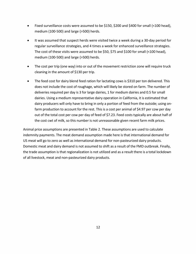
Animal price assumptions are presented in Table 2. These assumptions are used to calculate

indemnity payments. The meat demand assumption made here is that international demand for

US meat will go to zero as well as international demand for non-pasteurized dairy products.

Domestic meat and dairy demand is not assumed to shift as a result of the FMD outbreak. Finally,

the trade assumption is that regionalization is not utilized and as a result there is a total lockdown

of all livestock, meat and non-pasteurized dairy products.

13

Table 2. Market Price Assumptions

Animal Type Average Weight Average Market Price per Head

Steers: Stocker 600 lb class 654.00

Feeder 800 lb class 685.60

Fed 1000 lb class 857.00



Heifers: Stocker 600 lb class 644.00

Feeder 800 lb class 678.60




Milk Cow Replacement Heifer 1280

Cull Cow Dry Cow 400

Sheep Cull Ewe 160 lb 46.40

Replacement Ewe 80 lb 83.20

Ram 230 lb 66.70

Whether 90 lb 93.60

Male Feeder Lamb 60 lb 62.40

Female Feeder Lamb 50 lb 52.00

Hogs cull sows 215 lb 60.63

rep gilt 180 lb 79.56

boars 225 lb 99.45

feeder 140 lb 61.88

4.4. Herd Demographics

The breakdown of herd types is given in Table 3 from the DADS model. These groupings are

aggregated in ASM as: (1) Cow/Calf (2) Sheep (3) Dairy (4) Feeder Pig Production and (5) Hog

Farrow to Finish. Goats are captured in the sheep category, dairy calf operations are listed as

small feedlots, and backyard and saleyard are folded into the beef cattle categories. Table 4

provides their inventories and the total inventory of animals in the region of interest.

14

Table 3. Herd Definitions from DADS Model

Herd Type Definition

Large Beef More than 250 head beef cattle

Small Beef 1 to 250 head beef cattle Large Dairy More than 2000 head dairy cattle Medium Dairy 1001 to 1999 head dairy cattle Small Dairy 1 to 1000 head dairy cattle Large Dairy Calf More than 250 head dairy calves Small Dairy Calf 1 to 250 head dairy calves Large Swine More than 2000 head hogs Small Swine Less than 2000 head hogs Goat All size goat operations Sheep All size sheep operations Backyard Less than 10 head on premises Saleyards Mixed stock sale yard facilities

Table 4. Inventories of Animals in Susceptible Region When Moved to ASM

Operation Type Inventory (head)

Cow/Calf 911,805

Sheep 388,920 Dairy 1,382,305 Swine 45,594

TOTAL 2,728,624

In the DADS model, herd status is defined as susceptible, sub-clinically infectious, clinically

infectious, immune or dead. At the end of the outbreak period (day 120), it is assumed that all

infectious herds have been slaughtered or are destined to be slaughtered. Thus the "status"

variable is defined as either susceptible (status = 0) or dead (status = 3) when it enters the

economic part of the model. Susceptible implies that the herd is composed of animals that

could be infected with FMD and the herd lives in the Central Valley region, but at day 120 the

herd had not become infected with the disease. Dead implies that the herd was slaughtered for

disease control purposes.

15

5. Epidemic Model Results

Basic statistics for the epidemic model data across each scenario's 100 random trials were

calculated, including mean, standard deviation, coefficient of variation, median, min, max, and

25% and 75% probability intervals. The proportion of animals slaughtered or restricted out of

the total population represented by the approximately 22,000 livestock premises in California

that is modeled in the DADS model is also presented.

5.1. Animals Slaughtered for Disease Control

Summary statistics for the number of head slaughtered is presented in Table 5. For a graphical

representation, Figure 2. Spread of Disease Control Slaughter Distribution shows across the

different scenarios that slaughter will increase as the delay to detection increases but the

maximum of the number slaughtered distribution is reduced by the use of vaccination. These

results will motivate examination of delays in detection and slaughter later in the economic

results overview.

Table 5. Summary Statistics for Disease Control Slaughter1

Min 25% Median 75% Max Mean StDev

NoVacc_7Day 5 5,020 8,730 14,618 39,504 10,625 7,622

NoVacc_10Day 3,000 14,949 30,443 42,675 88,944 30,378 18,566

NoVacc_14Day 14,369 42,185 62,558 86,389 48,675 66,886 29,615

NoVacc_21Day 74,207 175,273 213,693 249,692 364,539 211,138 62,791

NoVacc_22Day 72,580 202,269 260,370 305,071 419,274 252,761 77,045

10Km_7Day 650 4,968 7,798 15,397 50,205 11,062 8,697

10Km_10Day 2,340 14,748 26,042 37,595 113,998 28,735 18,958

10Km_14Day 14,095 46,440 67,784 86,712 141,755 67,698 28,058

10Km_21Day 69,278 169,581 210,315 255,654 348,933 213,891 66,192

10Km_22Day 72,730 221,787 256,861 303,541 454,588 260,291 70,882

20Km_7Day 170 5,013 10,605 15,618 43,172 11,898 8,106

20Km_10Day 3,175 19,151 28,771 40,131 90,992 30,573 17,650

20Km_14Day 2,000 51,670 72,163 91,266 173,107 73,280 29,860

20Km_21Day 74,631 148,962 201,092 245,888 366,220 199,984 66,773

20Km_22Day 83,201 203,149 253,127 296,203 392,806 248,659 69,573

1 Variables for summary statistics tables are defined in Table 9.

16

Figure 2. Spread of Disease Control Slaughter Distribution2

5.2. Herds Placed Under Movement Restrictions

Summary statistics for the number of herds quarantined is presented in Table 6. Figure 3 shows

across the different scenarios the herds placed under movement restrictions will increase as

the delay to detection increases but the maximum herds restricted of the herds quarantined

distribution is decreased by vaccination.

2 For Figure 2 - Figure 4, the vertical line represents the spread from min to max, the square

indicates the 75th percentile, the circle represents the 25th percentile and the triangle represents

the median. The vertical axis is in number of head or herds as indicated in the text, and the

horizontal axis is the scenario considered. Variables are defined in Table 9.

17

Table 6. Summary Statistics for Herds Quarantined


NoVacc_7Day 73 401 677 1,092 4,728 968 881

NoVacc_10Day 169 873 1490 2,192 5,294 1,756 1,155

NoVacc_14Day 793 2,051 2,683 4,444 7,994 3,287 1,658

NoVacc_21Day 1,873 4,028 5,240 7,304 10,032 5,486 2,124

NoVacc_22Day 1,765 4,625 6,211 7,470 11,109 6,126 2,212

10Km_7Day 68 451 767 1,112 3,435 926 677

10Km_10Day 246 1,005 1,588 2,603 6,069 1,963 1,310

10Km_14Day 783 2,014 2,783 3,799 6,842 3,005 1,307

10Km_21Day 931 4,043 5,491 6,950 8,848 5,321 2,090

10Km_22Day 2,020 4,927 6,114 7,603 10,574 6,187 1,795

20Km_7Day 43 383 823 1,308 4,575 1,049 898

20Km_10Day 219 998 1,606 2,785 5,778 2,019 1,376

20Km_14Day 68 1,991 2,794 3,891 7,387 3,064 1,453

20Km_21Day 1,433 3,853 5,381 6,556 9,186 5,215 1,929

20Km_22Day 1,807 4,574 5,770 7,248 10,305 5,804 1,907

Figure 3. Spread of Herds Quarantined Distribution

18

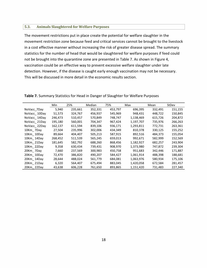
5.3. Animals Slaughtered for Welfare Purposes

The movement restrictions put in place create the potential for welfare slaughter in the

movement restriction zone because feed and critical services cannot be brought to the livestock

in a cost effective manner without increasing the risk of greater disease spread. The summary

statistics for the number of head that would be slaughtered for welfare purposes if feed could

not be brought into the quarantine zone are presented in Table 7. As shown in Figure 4,

vaccination could be an effective way to prevent excessive welfare slaughter under late

detection. However, if the disease is caught early enough vaccination may not be necessary.

This will be discussed in more detail in the economic results section.

Table 7. Summary Statistics for Head in Danger of Slaughter for Welfare Purposes


NoVacc_7Day 5,940 235,661 352,331 453,797 696,395 332,491 151,155

NoVacc_ 10Day 51,573 324,767 456,937 545,969 948,431 448,722 150,845

NoVacc_ 14Day 246,473 510,457 570,849 748,747 1,138,469 615,726 204,872

NoVacc_ 21Day 195,180 560,001 704,347 967,424 1,197,707 735,976 266,263

NoVacc_ 22Day 162,137 611,594 839,106 936,171 1,293,811 772,731 263,361

10Km_ 7Day 27,504 235,996 302,006 434,349 810,378 330,125 155,252

10Km_ 10Day 89,664 404,407 505,213 587,915 892,516 484,373 155,054

10Km_ 14Day 268,452 511,539 565,245 659,013 992,671 582,999 152,569

10Km_ 21Day 181,645 582,792 688,260 868,456 1,182,927 682,257 243,904

10Km_ 22Day 9,358 630,434 739,431 908,970 1,373,980 747,872 239,304

20Km_ 7Day 7,660 237,569 300,983 450,758 951,683 342,446 171,887

20Km_ 10Day 72,470 386,820 490,207 584,427 1,061,914 488,398 188,681

20Km_ 14Day 28,644 488,024 561,779 684,081 1,063,976 580,934 175,106

20Km_ 21Day 6,320 564,407 675,494 883,045 1,420,058 672,584 281,457

20Km_ 22Day 43,638 606,228 761,650 893,865 1,151,420 731,483 227,340

19

Figure 4. Spread of Head in Danger of Welfare Slaughter

6. Economic Model Results

The data above were used to adjust the sheep, cow/calf, dairy, farrow to finish, and feeder pig

production budgets in ASM in the outbreak region, Northern California in this case. All animals

infected were assumed to be slaughtered for disease control. Each of these groups will be

addressed separately.

In this study the FMD outbreak was restricted to the Northern California region (Figure 5).

However, since this region of California is a significant contributor to national supply of

livestock products and since the US is a significant player in the world market, effects will be felt

through the entire country and the rest of the world. The ASM model captures the change in

economic welfare3 or economic surplus from an animal disease because it calculates a dollar

loss of value added net income and a welfare cost of commodity prices rising. The trade

impacts are also be estimated within ASM. The results presented below include the trade

losses assuming the export of FMD affected, non-pasteurized products is closed for the entire

country for the remainder of the year after the outbreak is brought under control.

3 Economic welfare loss is the loss in the aggregate well-being of participants in a market based

on alternative allocations of scarce resources. This is sometimes referred to as economic surplus.

The second term will be used here to prevent confusion with the term welfare slaughter.

20

Figure 5. ASM Sub-Regional Breakdown of California

6.1. National Agricultural Economic Surplus Impacts Under Alternative Delays in

Detection and Vaccination

Examining results first from a national level, the change in total agricultural economic surplus is

examined resulting from the outbreak. These results include international trade impacts, but do

not examine a policy of regionalization of production to limit trade impacts. Table 8, Table 9,

and Table 10 provide summary statistics for each of the alternative scenarios where losses are

measured in millions of year 2004 dollars. As detection of the disease is delayed, median losses

increase. Furthermore, median loss under vaccination exceeds losses under no vaccination. This

is due to the increased slaughter and costs accompanying a vaccination scenario.

21

Table 8. Summary Statistics for National Loss in Total Agricultural Surplus-No Vaccination

(Millions of 2004$)

NoVacc_7Day NoVacc_10Day NoVacc_14Day NoVacc_21Day NoVacc_22Day

Mean -2,700.15 -7,234.44 -15,955.49 -52,773.11 -64,690.18

StDev 2,064.24 4,985.89 8,980.83 23,399.11 29,789.40

95 % LCI -3,169.90 -8,369.06 -17,999.22 -58,097.94 -71,469.21

95 % UCI -2,230.40 -6,099.83 -13,911.77 -47,448.29 -57,911.15

Min -10,712.43 -22,841.37 -41,302.48 -103,456.86 -129,949.90

Median -2,292.40 -7,105.06 -15,234.25 -55,433.41 -68,980.89

Max 34.05 34.05 34.05 29.87 -13.83


Vaccination (Millions of 2004$)

10Km_7Day 10Km_10Day 10Km_14Day 10Km_21Day 10Km_22Day

Mean -3,956.72 -9,328.42 -19,724.10 -60,253.28 -74,859.55

StDev 3,055.83 6,255.07 9,568.56 26,957.88 31,680.93

95 % LCI -4,652.12 -10,751.86 -21,901.57 -66,387.95 -82,069.03

95 % UCI -3,261.31 -7,904.99 -17,546.62 -54,118.60 -67,650.08

Min -15,322.41 -35,228.20 -44,211.64 -112,697.26 -149,809.74

Median -3,128.46 -9,359.11 -19,460.55 -60,683.94 -76,907.02

Max 34.05 34.05 34.05 29.87 -15.28


Vaccination (Millions of 2004$)

20Km_7Day 20Km_10Day 20Km_14Day 20Km_21Day 20Km_22Day

Mean -4,954.40 -10,546.03 -21,907.81 -50,091.27 -71,682.91

StDev 3,301.69 6,279.97 10,670.21 31,551.89 30,347.65

95 % LCI -5,705.75 -11,975.14 -24,335.98 -57,271.38 -78,588.98

95 % UCI -4,203.05 -9,116.93 -19,479.64 -42,911.16 -64,776.84

Min -13,927.17 -26,563.21 -53,727.52 -121,195.84 -125,492.53

Median -4,776.39 -10,880.95 -22,772.48 -55,622.56 -78,792.09

Max 34.05 34.05 34.05 29.87 -15.28

22

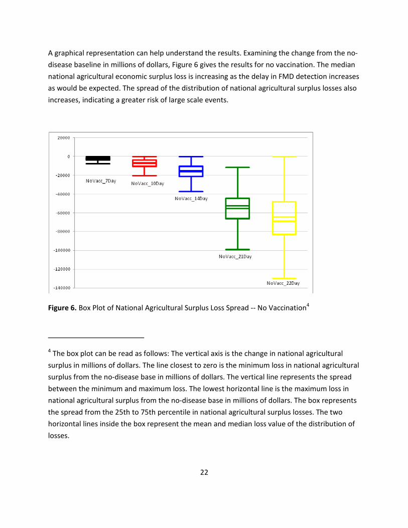
A graphical representation can help understand the results. Examining the change from the no-

disease baseline in millions of dollars, Figure 6 gives the results for no vaccination. The median

national agricultural economic surplus loss is increasing as the delay in FMD detection increases

as would be expected. The spread of the distribution of national agricultural surplus losses also

increases, indicating a greater risk of large scale events.

Figure 6. Box Plot of National Agricultural Surplus Loss Spread -- No Vaccination4

4 The box plot can be read as follows: The vertical axis is the change in national agricultural

surplus in millions of dollars. The line closest to zero is the minimum loss in national agricultural

surplus from the no-disease base in millions of dollars. The vertical line represents the spread

between the minimum and maximum loss. The lowest horizontal line is the maximum loss in

national agricultural surplus from the no-disease base in millions of dollars. The box represents

the spread from the 25th to 75th percentile in national agricultural surplus losses. The two

horizontal lines inside the box represent the mean and median loss value of the distribution of

losses.

23

When vaccination is used as a way of controlling the spread of the disease, the same pattern is

seen but with a greater success in reducing the spread of national agricultural surplus losses.

Figure 7 shows results when 10 km ring vaccination is employed and Figure 8 shows results

when 20 km ring vaccination is employed. Under the latest days to detection (21 and 22) the 10

kilometer ring vaccination is not as successful in reducing the spread of national agricultural

surplus loss as the 20 kilometer ring vaccination. However, the mean and median national

agricultural surplus loss is not reduced by vaccination. Based on these results, 20 kilometer ring

vaccination would be a viable control strategy to minimize national agricultural surplus losses

under late detection if decision makers wish to reduce the probability of an extreme outcome,

but does not appear to provide any additional benefits under earlier detection scenarios or in

reducing mean and median national agricultural surplus losses.

Figure 7. Box Plot of National Agricultural Surplus Loss Spread -- 10 Km Ring Vaccination

24

Figure 8. Box Plot of National Agricultural Surplus Loss Spread -- 20 Km Ring Vaccination

Clearly, the vaccination policy would be set without clear knowledge of how many days might

expire before the disease is detected. Figure 9 shows the box plot of national agricultural

surplus losses under alternative vaccination strategies across all delays in detection. While 10

km ring vaccination does not provide benefits outweighing the costs in terms of additional

slaughter required (recall the "vaccinate to die" assumption) and additional costs of disease

mitigation, it appears 20 km ring vaccination does provide sufficient benefits to reduce the

spread of national agricultural surplus losses. Even 20 km ring vaccination does not appear to

reduce the mean or median national surplus loss. Thus in this particular study, vaccination of

dairy herds in a 20 km ring around infected premises is not a viable policy for slowing the

spread of the disease and minimizing the mean or median national surplus losses from the

disease. It may however, be a viable option for reducing the chance of an extreme disease

outcome occurring.

25

Figure 9. Box Plot of National Agricultural Surplus Loss Spread Under Alternative Vaccination

6.2. Risk Aversion Analysis

Under alternative delays in detection, earlier detection is always preferred to later detection

across all risk neutral and risk averse individuals. This corresponds to prior studies that have

consistently found early detection to be preferable to later detection as a way of reducing the

duration of an FMD outbreak, the level of slaughter employed to eradicate the disease, and the

national costs of controlling the disease.

Vaccination has both pros and cons. First under current "vaccinate to die" strategy more

slaughter is employed and second vaccination is costly in terms of supplies and man-hours.

However, the goal of vaccination is to slow the spread of the disease. Thus, it should be

examined as a risk reduction technique. Stochastic Efficiency with Respect to a Function (SERF)

is used here. The SERF method identifies where dominance between two alternatives switches

(breakeven risk aversion coefficients) given bounds on the absolute risk aversion coefficient

(ARAC). SERF allows for estimation of the utility-weighted risk premiums between alternatives

to provide a cardinal measure for comparing the payoffs between risky alternatives (Hardaker

et al.). Figure 10 presents the SERF diagram showing that the highest expected utility is

obtained from 20 Km vaccination as the ARAC rises. For vaccination, as risk aversion rises

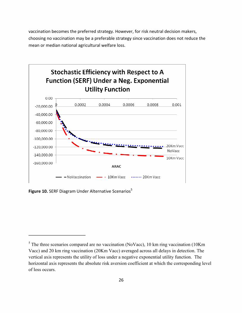
26

vaccination becomes the preferred strategy. However, for risk neutral decision makers,

choosing no vaccination may be a preferable strategy since vaccination does not reduce the

mean or median national agricultural welfare loss.

Figure 10. SERF Diagram Under Alternative Scenarios5

5 The three scenarios compared are no vaccination (NoVacc), 10 km ring vaccination (10Km

Vacc) and 20 km ring vaccination (20Km Vacc) averaged across all delays in detection. The

vertical axis represents the utility of loss under a negative exponential utility function. The

horizontal axis represents the absolute risk aversion coefficient at which the corresponding level

of loss occurs.

27

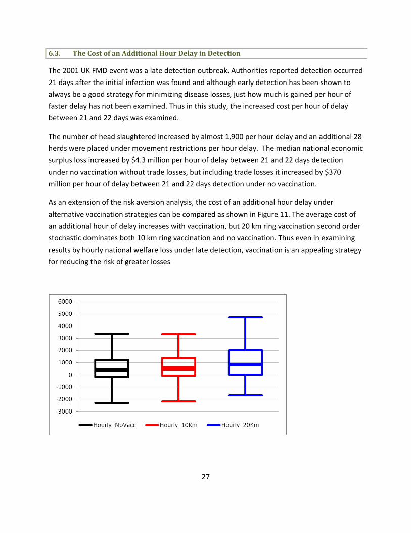
6.3. The Cost of an Additional Hour Delay in Detection

The 2001 UK FMD event was a late detection outbreak. Authorities reported detection occurred

21 days after the initial infection was found and although early detection has been shown to

always be a good strategy for minimizing disease losses, just how much is gained per hour of

faster delay has not been examined. Thus in this study, the increased cost per hour of delay

between 21 and 22 days was examined.

The number of head slaughtered increased by almost 1,900 per hour delay and an additional 28

herds were placed under movement restrictions per hour delay. The median national economic

surplus loss increased by $4.3 million per hour of delay between 21 and 22 days detection

under no vaccination without trade losses, but including trade losses it increased by $370

million per hour of delay between 21 and 22 days detection under no vaccination.

As an extension of the risk aversion analysis, the cost of an additional hour delay under

alternative vaccination strategies can be compared as shown in Figure 11. The average cost of

an additional hour of delay increases with vaccination, but 20 km ring vaccination second order

stochastic dominates both 10 km ring vaccination and no vaccination. Thus even in examining

results by hourly national welfare loss under late detection, vaccination is an appealing strategy

for reducing the risk of greater losses

28

Figure 11. Box Plot of Cost per Hour of Delay between 21 and 22 Days

6.4. Price Impacts

Price impacts under this set of assumptions are driven by the reduction in supply associated

with slaughter and trade restrictions. Results are broken out by live animal impacts, meat and

livestock impacts excluding dairy, dairy price impacts and price impacts for feed grains.

1.1.8. Price Impacts for Live Animals

Recall that ASM is acting almost as a short run equilibrium model where price and quantity

changes are a reflection of the animal disease shock but herd adjustments are not allowed.

There are two sources of movement in live animal prices. The first is obviously the shift in

supply resulting from massive slaughter of animals in California, dairy calves in particular. The

second, forces driving quantity demanded and supplied in other regions such as a greater

surplus of grain available for feeding and increased domestic meat prices due to international

trade restrictions. These two forces will be moving against each other, and the direction of the

price change expected will depend on the relative sizes of these shifting factors. Table 11

provides results across all vaccination levels for beef animals.

Other than dairy production operations, feeding operations for dairy calves and some beef

calves make up the remainder of cattle production in California. The majority of cattle feeding

occurs in lower Sacramento, San Joaquin and Imperial Valleys (CCA). Simulation results indicate

a reduction in the number of yearlings and fed cattle in the region, but this is offset by an

increase in the production of yearlings and fed cattle in other regions (particularly the Great

Plains). The increase in production in other regions could be from lower feed prices

encouraging expansions in feeding operations or increased imports to take advantage of higher

domestic fed beef prices, which in turn pulls up prices on yearlings and slaughter cattle.

For cow/calf operations, a supply shift from California will not significantly change the

aggregate national supply of beef animals. California had only 662,423 beef cows in their

national inventory as of 2007 (USDA-NASS, 2008). National cow/calf quantity is not affected

enough to shift aggregate supply of calves or stockers. However, demand for calves and

stockers would change due to effects trickling down from changes in calf demand in feeding

operations and supply changes in other regions, resulting in a lower price for calves.

29

Table 11. Mean Prices of Live Cattle Under Alternative Days of Detection6

Mean Feedlot

Beef

Slaughter

Steer

Calve

Heifer

Calves

Stocked

Calf

Stocked

HCalf

Stocked

SCalf

Dairy

Calves

Stocked

Yearling

Base 73.554 122.206 130.051 87.129 103.329 103.212 122.206 85.356

7Day 73.554 118.114 117.432 84.060 103.291 103.017 119.922 87.751

10Day 73.554 118.125 118.214 84.069 103.432 103.081 119.930 89.440

14Day 73.554 118.140 119.231 84.082 103.595 103.123 119.945 90.244

21Day 73.728 118.623 121.195 84.447 103.622 103.128 120.443 89.474

22Day 73.962 119.257 122.293 84.927 103.656 103.133 121.096 89.267

California is not a major producer of hogs and pigs, ranking 29th in the nation (USDA-NASS,

2009). However, international trade restrictions without the use of zoning implies that pork will

also be a restricted commodity. The US is a major exporter of pork, so a block of pork exports

means lower demand for hogs for slaughter and feeder pigs. Price changes in these

commodities reflect these adjustments. California is ranked third in sheep and goat production,

but with no trade impacts and relatively small quantity impacts in the region in question there

is not enough market forces being brought to bear in order to shift lamb or mutton prices.

Table 12 provides results across all vaccination levels for hogs and sheep.

Table 12. Mean Prices of Live Hogs and Sheep Under Alternative Days of Detection

Mean HogsforSlaughter FeederPig CullSow LambSlaugh CullEwes

Base 66.681 122.009 38.906 47.457 22.545

7Day 66.5882 121.26801 38.8452 47.457 22.545

10Day 66.561 121.12786 38.8273 47.457 22.545

14Day 66.5546 121.09496 38.8231 47.457 22.545

21Day 66.5658 121.15661 38.8304 47.457 22.545

22Day 66.5674 121.16923 38.8315 47.457 22.545

6 Variables are delays in detection averaged across all vaccination scenarios.

30

Although poultry production is not affected by FMD directly, chicken and turkey serve as a

substitute for beef and a complement for pork (Davis et al.). Thus demand effects will be

moving in opposite directions as a result of an FMD outbreak. The direction of the price change

will depend on which is larger. The change in the price of chicken and turkey will determine the

changes in the price of broilers, turkeys and eggs. The next section provides an overview of

these results. Table 13 provides the prices changes in eggs, broilers and turkeys.

Table 13. Mean Prices of Eggs and Live Poultry Under Alternative Days of Detection

Mean Eggs Broilers Turkeys

Base 0.919 47.219 54.894

7Day 0.915 47.433 55.318

10Day 0.915 47.433 55.318

14Day 0.915 47.433 55.318

21Day 0.915 47.433 54.495

22Day 0.915 46.778 54.495

1.1.9. Price Impacts for Meat and Livestock Products Excluding Dairy

A key assumption that is worth stating again is that domestic meat consumption is not reduced

due to "fear factors" about meat safety. Rather, price changes are driven by supply shifts in live

animals and international trade impacts. Table 14 provides prices for beef, pork and poultry

over all vaccination scenarios. For beef, changes in national supply were apparently small

enough to not affect price in the earlier days to detection but does increase price under the

latest detection scenarios. Pork price however, most likely due to the international trade

impacts, is reduced. Chicken and turkey prices are increased under early detection scenarios;

however, under 22 day detection chicken price decreases below the pre-disease base and

under 21 and 22 day detection turkey price decreases below the pre-disease base. This may be

reflective of the role of poultry as a substitute for beef. One other commodity price that could

be mentioned here is the price of wool. As the number of sheep is reduced, the supply of wool

available will decrease and consequently the price of wool is increased as shown in Table 15.

31

Table 14. Mean Prices of Beef, Pork and Poultry Under Alternative Days to Detection

Mean FedBeef Pork Chicken Turkey

Base 127.2 79.12500 61.069 75.208

7Day 127.2 79.00023 61.337 75.805

10Day 127.2 78.96373 61.337 75.805

14Day 127.2 78.95515 61.337 75.805

21Day 127.5 78.97017 61.337 74.644

22Day 127.8 78.97232 60.518 74.644

Table 15. Mean Price of Wool Under Alternative Days to Detection

Mean WoolClean

Base 0.739

7Day 0.739

10Day 0.739

14Day 0.739

21Day 0.740

22Day 0.740

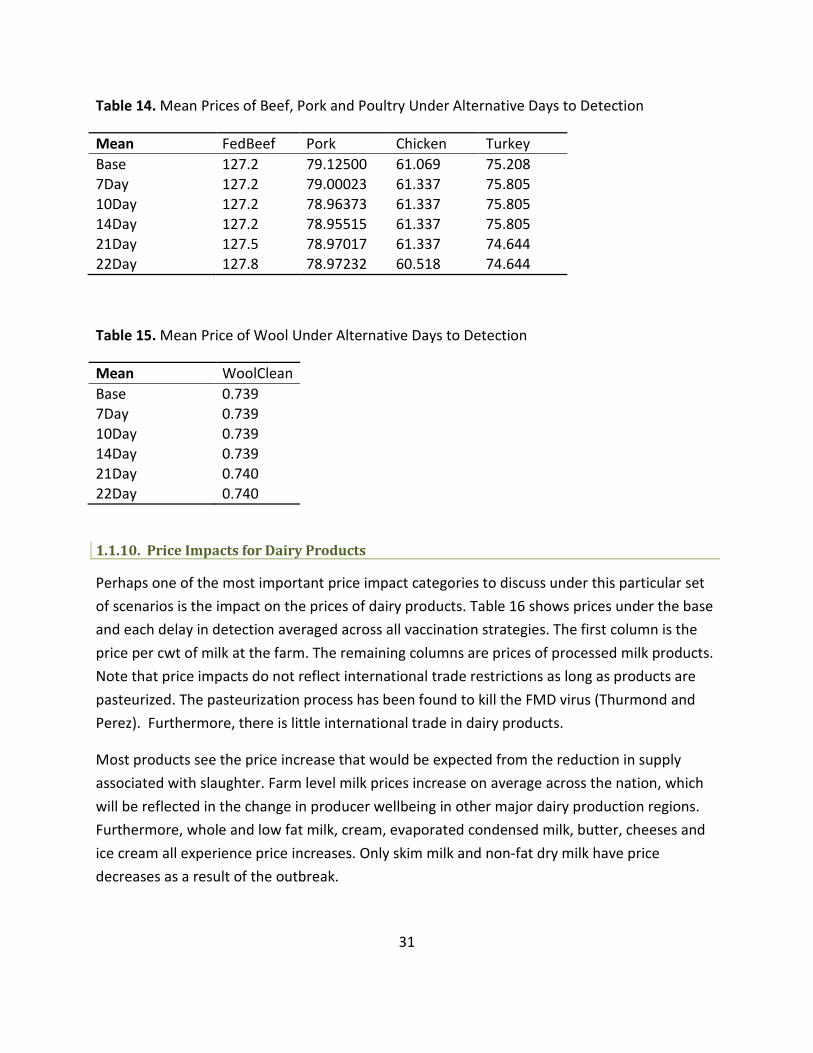
1.1.10. Price Impacts for Dairy Products

Perhaps one of the most important price impact categories to discuss under this particular set

of scenarios is the impact on the prices of dairy products. Table 16 shows prices under the base

and each delay in detection averaged across all vaccination strategies. The first column is the

price per cwt of milk at the farm. The remaining columns are prices of processed milk products.

Note that price impacts do not reflect international trade restrictions as long as products are

pasteurized. The pasteurization process has been found to kill the FMD virus (Thurmond and

Perez). Furthermore, there is little international trade in dairy products.

Most products see the price increase that would be expected from the reduction in supply

associated with slaughter. Farm level milk prices increase on average across the nation, which

will be reflected in the change in producer wellbeing in other major dairy production regions.

Furthermore, whole and low fat milk, cream, evaporated condensed milk, butter, cheeses and

ice cream all experience price increases. Only skim milk and non-fat dry milk have price

decreases as a result of the outbreak.

32

Table 16. Mean Price of Dairy Products Under Alternative Days to Detection

Mean

Milk Fluid

Milk-Whole

Fluid Milk

Low-Fat

Skim Milk Cream Evap CondM

Base 14.927 0.3350 0.3120 0.1330 0.690 0.349

7Day 15.049 0.3359 0.3121 0.1330 0.706 0.354

10Day 15.136 0.3363 0.3126 0.1329 0.717 0.357

14Day 15.362 0.3375 0.3131 0.1326 0.746 0.365

21Day 15.977 0.3404 0.3143 0.1316 0.823 0.387

22Day 16.144 0.3412 0.3148 0.1315 0.843 0.392

Mean

Non Fat Dry Milk Butter Amer Cheese Other Cheese Cottage Cheese Ice Cream

Base 1.1470 1.4020 1.7600 2.0210 1.5950 1.8380

7Day 1.1444 1.4366 1.7720 2.0291 1.5974 1.8675

10Day 1.1423 1.4614 1.7808 2.0349 1.5994 1.8883

14Day 1.1368 1.5260 1.8035 2.0499 1.6046 1.9423

21Day 1.1224 1.7009 1.8650 2.0910 1.6189 2.0888

22Day 1.1206 1.7444 1.8818 2.1024 1.6227 2.1261

1.1.11. Price Impacts for Feed Grains

A final price impact category that usually receives little attention is feed grains. Feed grain price

changes are the result of changes in demand for feed grains when livestock operations are

subject to a disease outbreak. Slaughter in California means a reduction in the demand for feed

grain in that region, which in turn results in additional supply for other regions. This is reflected

in the decrease in feed grain prices shown in Table 17.

Table 17. Mean Price of Feed Grains Under Alternative Days to Detection

Mean Corn for

Beef Cattle

Corn for

Dairy Cattle

Corn for

Hogs

Corn for

Poultry

Base 4.6160 4.40000 4.5770 4.44100

7Day 4.6087 4.39516 4.5727 4.43856

10Day 4.6083 4.39445 4.5723 4.43825

14Day 4.6080 4.39428 4.5722 4.43819

21Day 4.6076 4.39439 4.5723 4.43826

22Day 4.6075 4.39427 4.5722 4.43818

33

1.1.12. Summary of Price Changes

Intuitively, these price changes could reflect the following scenario. The supply of dairy

products goes down as well as the supply of calves coming from California. Fed cattle numbers

go up nationally, possibly supplemented by increased imports of live animals, fueled by the

higher price of beef compounded with lower grain prices caused by a surplus of unused grain

originally destined for cattle use. The supply decrease in domestic fed cattle and yearlings is

more than offset by increased demand for fed cattle and yearlings. However, since imports are

still allowed from Canada and Mexico, this demand effect does not appear to trickle down into

grazing operations (stockers and calves), which just experience the supply shift resulting in

lower prices of stockers and calves.

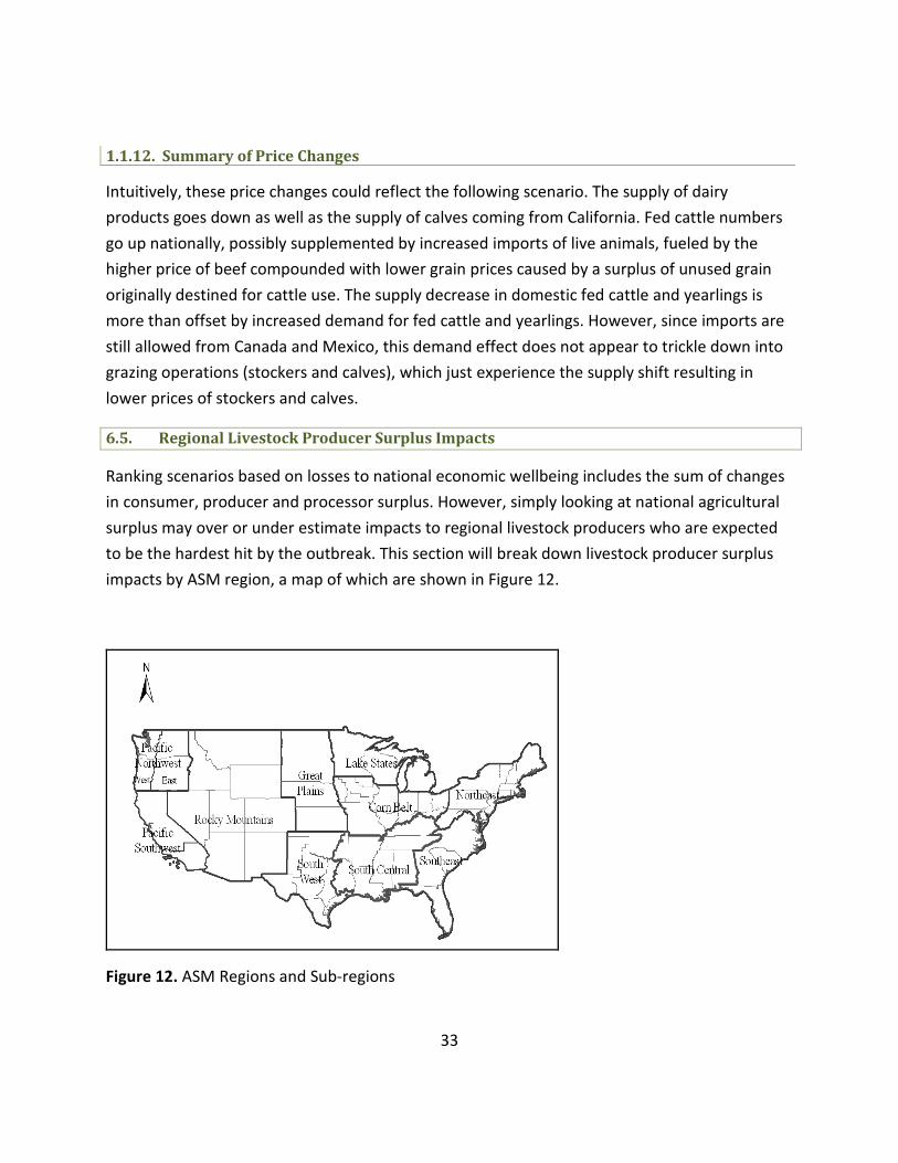
6.5. Regional Livestock Producer Surplus Impacts

Ranking scenarios based on losses to national economic wellbeing includes the sum of changes

in consumer, producer and processor surplus. However, simply looking at national agricultural

surplus may over or under estimate impacts to regional livestock producers who are expected

to be the hardest hit by the outbreak. This section will break down livestock producer surplus

impacts by ASM region, a map of which are shown in Figure 12.

Figure 12. ASM Regions and Sub-regions

34

Based on what is known about production demographics in various parts of the country, the

following analysis examines individual regions to determine those who gain and those who lose

from the disease. Note, when the term "producer" is used in this section it means livestock

producers not all agricultural producers including crop farmers.

1.1.13. Total US Livestock Producer Surplus Changes

When looking at the change in producer surplus in the nation as a whole, the median loss from

a no disease base is $15.8 billion as shown in Table 18. Summary Statistics for Total Livestock

Producers' Surplus Changes Relative to the Base. Comparing across delays in detection for all

vaccination types, early detection still second order stochastic dominates late detection. This

implies that producers should have an incentive to participate in earlier detection if it is clear

the losses that could be sustained from later detection. Comparing across different vaccination

strategies, a different ranking is discovered. Producers prefer that vaccination not be used

during the outbreak, followed by 20 km ring vaccination. Only under the latest detection

scenario, when risk aversion is increasing does 20 km ring vaccination become preferred to no

vaccination. This is not unreasonable from a producer standpoint given the additional slaughter

inherent in the use of vaccination. Examining the producer surplus loss in the nation as a whole

may underestimate the producer impacts in the infected region, so the remainder of this

section will examine the producer impacts region by region.

Table 18. Summary Statistics for Total Livestock Producers' Surplus Changes Relative to the

Base Scenario7

Mean StDev Min Median Max

Total_7Day (3,590.50) 2901.029842 (14,521.48) (2,879.86) 142.98

Total_10Day (8,601.54) 5803.350086 (33,790.68) (8,649.68) 142.98

Total_14Day (18,350.00) 9635.195504 (51,795.76) (18,583.05) 142.98

Total_21Day (52,438.08) 26895.06769 (118,096.74) (55,095.09) 143.18

Total_22Day (68,298.85) 29995.8705 (146,141.28) (72,506.45) (81.73)

7 Variables are the total US economic surplus change averaged across alternative vaccination

strategies for delays in detection.

35

1.1.14. Pacific Southwest (PSW)

Starting with the region of outbreak it can reasonably be expected that producers’ wellbeing in

this region will fall more than in any other region. As expected the median change in national

producer surplus from the no-disease base is $16.5 billion as shown in Table 19. This is the

largest loss region in the simulated outbreak under all scenarios. Comparing this to the total US

producer surplus change, not examining this region individually would underestimate the loss

producers would face. Rankings of strategies remain the same. Early detection is always

preferred to later detection and no vaccination is the preferred strategy unless detection occurs

late and decision makers are more risk averse.

Table 19. Summary Statistics for California (Pacific Southwest) Livestock Producers' Surplus

Changes Relative to the Base Scenario


PSW_7Day (3,860.17) 2965.57 (15,188.63) (3,197.30) (26.60)

PSW_10Day (8,979.70) 5951.003 (34,888.22) (8,980.65) (26.60)

PSW_14Day (19,025.03) 9927.107 (53,264.65) (19,160.05) (26.60)

PSW_21Day (53,927.82) 27540.89 (120,504.57) (56,798.49) (24.33)

PSW_22Day (69,855.60) 30620.06 (148,931.84) (74,348.53) (33.23)

1.1.15. Dairy Producing Regions

As stated earlier, California is the top dairy producing state in the US followed by Wisconsin

(which resides in the Lake States region), New York, Pennsylvania (which are both in the

Northeast region), and Idaho (which is in the Rocky Mountains region). Given the decrease in

dairy coming from California as a result of the outbreak, there is a strong potential that

producers in these regions could gain as a result of higher dairy prices. As shown in Table 20,

under all delays in detection and vaccination strategies, the producers in the Lake States (LS)

and Northeast (NE) regions gain from the outbreak. Producer surplus gains in the LS region

ranged from a median $35 million under the earliest detection scenario to $372 million under

the latest detection scenario, in which dairy prices are highest.

Results in the Rocky Mountain (RM) region were more mixed. Median producers surplus in the

RM region falls under early detection at 7 days by $35 million; however, it should be noted that

36

some of the cattle production in California is shipped to Idaho to be fed out. Starting with

detection at 10 days though, simulations indicate producers begin to gain in median surplus.

This gain ranges from $7.6 million at 10 days to $469 million at 22 days.

Table 20. Summary Statistics for Other Dairy Producing Regions Livestock Producers' Surplus

Changes Relative to the Base Scenario8


LS_7Day 40.34 15.90662 5.45 35.92 103.06

LS_10Day 62.36 33.09408 5.45 57.96 208.16

LS_14Day 120.31 60.93538 5.45 108.34 281.77

LS_21Day 274.58 125.5223 0.92 315.02 435.73

LS_22Day 318.85 117.2334 0.25 372.59 544.38

NE_7Day 21.85 12.93702 (6.01) 18.00 72.74

NE_10Day 40.10 27.04435 (6.01) 37.00 159.50

NE_14Day 87.58 49.56092 (6.01) 77.16 218.98

NE_21Day 216.45 102.0455 (6.49) 249.03 347.06

NE_22Day 245.99 95.34417 (13.55) 288.97 429.32

RM_7Day (35.07) 29.25864 (92.95) (46.14) 91.33

RM_10Day 7.68 58.28563 (92.95) 4.69 258.78

RM_14Day 108.82 101.9264 (92.95) 100.51 372.48

RM_21Day 379.94 217.4802 (95.04) 443.59 692.07

RM_22Day 469.19 210.46 (95.06) 534.19 866.20

1.1.16. Other Livestock and Grain Production Regions

Regions that are major producers of cattle largely realized gains from the disease outbreak. This

includes the Great Plains (GP) region that realized gains in median producer surplus ranging

from $282 million under 14 day delay in detection to $320 million under 22 day detection--the

region also had gains at 7, 10 and 21 days delay. This region houses a thriving cow/calf and

8 Here the Lake States region is abbreviated LS, the Northeastern region is abbreviated NE and

the Rocky Mountain region is abbreviated RM.

37

cattle feeding industry as well as grain production. Producers in that region stand to benefit

from lower grain prices for cattle and increased prices for fed cattle resulting from the

outbreak. Results are shown in Table 21.

Table 21. Summary Statistics for Great Plains Region Livestock Producers' Surplus Changes

Relative to the Base Scenario


GP_7Day 300.47 12.37781 249.56 307.35 315.62

GP_10Day 289.19 16.72731 238.40 287.75 319.25

GP_14Day 282.78 18.05414 239.45 287.03 317.80

GP_21Day 300.59 36.94364 229.46 299.61 384.63

GP_22Day 316.65 40.06479 222.26 320.91 379.60

Producers in the Southwest (SW) region realize a small loss in producers surplus at 7 day delay

in detection of $4 million, but realize gains under later detection ranging from $2 million at 10

day delay in detection to $64 million at 22 day delay in detection. Dairy producers in the region

will gain from higher milk and dairy product prices and lower grain prices. Fed beef operations

will gain from lower grain prices and higher fed beef prices resulting from the outbreak.

Results are shown in Table 22.

Table 22. Summary Statistics for Southwest Region Livestock Producers' Surplus Changes



SW_7Day (4.05) 6.955987105 (14.81) (4.02) 17.96

SW_10Day 2.41 9.423441148 (14.81) 1.96 32.81

SW_14Day 15.58 13.24821979 (14.81) 17.05 46.79

SW_21Day 49.58 30.18861476 (15.67) 53.26 109.51

SW_22Day 59.10 31.94402985 (21.85) 64.41 111.54

The Corn Belt (CB) is where the majority of the hog production in the US occurs. As such, this

region experiences losses in median producer surplus ranging from $4.7 million at 22 days delay

38

in detection to $28.5 million at 7 days delay in detection. These losses will most likely occur as a

result of the trade restriction moving the price of hogs and pork down, although it may be

partially offset by the decrease in the price paid for feed corn. Results are shown in Table 23.

Table 23. Summary Statistics for Corn Belt Region Livestock Producers' Surplus Changes Relative

to the Base Scenario


CB_7Day (8.17) 31.10313 (33.31) (28.54) 41.25

CB_10Day (10.39) 29.34425 (33.31) (27.55) 45.58

CB_14Day (7.46) 29.14301 (33.31) (21.11) 50.85

CB_21Day 4.09 31.47634 (34.84) (6.99) 66.18

CB_22Day 7.98 31.26028 (35.14) (4.74) 69.03

Producers in the South Central region of the US lose in median surplus under these simulated

outbreaks except for under a 21 day delay in detection. This may be due to the mixed

production in that region, with losses resulting from cow/calf production impacts. Results are

shown in Table 24.

Table 24. Summary Statistics for South Central Region Livestock Producers' Surplus Changes



SC_7Day (47.17) 6.947994686 (58.98) (49.80) (16.39)

SC_10Day (37.21) 12.53958739 (58.98) (36.79) 14.53

SC_14Day (15.97) 20.68908048 (58.98) (14.97) 33.64

SC_21Day 35.23 47.36841891 (64.66) 44.25 115.77

SC_22Day (72.62) 49.13154456 (196.10) (70.66) 14.33

The Southeast region covering Florida, Georgia, North and South Carolina and Virginia will have

producers gaining in median wellbeing by a small amount under each scenario except for the 7

day delay in detection as shown in Table 25. These results, like the South Central region may be

mixed due to the mix of livestock producer types in the region. Florida, in particular is a large

39

cattle production state but North Carolina is a large hog production state. Thus the impact on

this region will vary depending on the size of the outbreak. At only a 7 day delay in detection,

the trade impact to hog production appears to be outweighing the impact to cattle and poultry

producers.

Table 25. Summary Statistics for Southeast Region Livestock Producers' Surplus Changes



SE_7Day 0.54 16.93687 (27.51) (1.31) 53.82

SE_10Day 10.66 21.32897 (27.51) 5.00 83.00

SE_14Day 38.85 32.21059 (27.51) 39.66 116.72

SE_21Day 100.96 66.44067 (46.55) 120.58 217.94

SE_22Day 59.14 64.31642 (115.29) 82.61 171.37

6.6. Trade Impact Analysis

Results from an animal disease outbreak must include trade impacts to truly measure the

extent of the outbreak impacts. Trade impacts are a demand side shift that is fairly certain since

it is a proven policy when countries have a case of FMD within the borders. The extent and

duration are uncertain though. Although the results presented here are including trade

impacts, this may actually be a "worst case scenario" of the trade impacts. The likelihood of

having a lockdown of all non-pasteurized livestock products for a full year even though the

disease is contained within a few months is somewhat unlikely.

First, there is the possibility of zoning the disease to a particular region. In this study, zoning

might mean that because the disease is contained in California only California exports arising

from California would be restricted. This certainly would reduce impacts related to pork since

California is such a small producers of this commodity, which makes up a large expected trade

impact. Even if zoning were not utilized, some trade may be resumed before the end of the

year where this assumes the remainder of the year trade restrictions will be in place.

Second, trade analysis was not taken out into future years since trade restrictions remain in

place at some level 2-5 years into the future. This only looks at year 0, the year of the outbreak.

In particular, for the use of vaccination trade will be restricted longer since the US would have a

40

"FMD Free with Vaccination" status for several years. This may warrant allowing the ASM

model to find a dynamic equilibrium since longer term trade restrictions may alter the livestock

industry in the US. The future years of the restrictions would need to be considered to truly

assess the disease outbreak with full trade impacts. The limitations described in this section

could be explored in a separate extension of the study.

7. Conclusions and Implications

This study of the California Central Valley provides results that are comparable to other

economic studies of FMD done in that region, but the use of an integrated epidemic-economic

framework provides greater detail that was has previously been provided. A study done by

Ekboir provides a useful frame of reference as well as the most recent census of agriculture in

California. This section will briefly provide evidence as to the reasonableness of results. Ekboir

estimated the total cost of the outbreak to range from $6.7 to $13.5 billion in 1999. This did not

include price changes and national economic surplus changes since his model was an

input/output model. Thus this report is not only an update of the impacts of FMD in California,

but also a more thorough examination compared to prior studies.

The median amount of disease related slaughter, herds under movement restriction and

potential welfare slaughter increases as the delay in detection increases. Vaccination increases

the median slaughter, but reduces the median number of herds subject to movement

restrictions and consequently in danger of welfare slaughter. Vaccination does however appear

to reduce the tail of the distribution of animals placed under movement restrictions.

National economic surplus losses increase as the delays in detection increase and also increase

at the median with vaccination; however, when risk aversion is taken into account 20 kilometer

ring vaccination becomes a preferred strategy as risk aversion rises. This indicates that policy

makers may be willing to implement a policy with a higher median loss in order to avoid an

extreme outcome.

Producers in California clearly suffer the largest levels of losses in the country from an outbreak

in that region. However if only the national levels of welfare are examined, the losses to that

region may be underestimated since other producers in the country gain from higher prices and

lower feed grain costs. Similarly if only regional effects are considered without consideration of

price changes than the losses will be overstated.

41

In terms of limitations, there is still much work that could be done for animal disease modeling.

In particular the approach and analysis in this study could be improved by considering several

factors. First, the international trade assumptions could be improved. The assumption is that

the disease is confined to California but that all US opportunities to export were lost. However a

zoning policy might be able to be employed to reduce international trade losses. In particular,

the pork trade would not be as affected if zoning were put into place. The assumption that

livestock and livestock product exports are reduced to autarky levels is a worst case scenario

that would be more applicable to a multi-region outbreak rather than a regionalized outbreak.

Second, only the short run aspects of the outbreak were examined. Essentially, the "year 0" or

the year of the outbreak were examined without looking the 5-10 years into the future to

determine when or if the livestock sector would recover from the outbreak. This long run

analysis would particularly be important given international trade impacts and the time it will

take to regain market share after export restrictions are put in place by our current export

partners.

In terms of further work, what is clear is that the threat of animal disease--FMD in particular--is

very real to the US agricultural sector and there is still much work to be done to assess

vulnerability and outbreak related strategies would be over the short and long run. Further

aspects not discussed in this study, but that could be examined in the future, are the

implications this would have on tourism and commercial traffic important to the California

economy. Furthermore, the costs of human suffering and lost wages from movement

restriction policies could be explored. Also the results could be extended by explorations of the

balance between ex ante investment and ex post response. In order to have early detection,

investment would need to be made in diagnostics equipment and personnel in laboratories as

well as the possibility of a random, mandatory testing procedure in vulnerable regions.

Although these issues are not specifically modeled in this dissertation, the results presented

here provide motivation for the further examination of balance issues.

42

8. References

Adams, D., R. Alig, B.A. McCarl, and B.C. Murray. "FASOMGHG Conceptual Structure, and

Specification: Documentation." Unpublished manuscript, Texas A&M University, February,

2005.

Anderson, I. “Foot and Mouth Disease 2001: Lessons to be Learned Inquiry Report.” Internet

site: http://archive.cabinetoffice.gov.uk/fmd/fmd_report/index.htm (Accessed December

1, 2002).

Bates, T.W., M.C. Thurmond, and T.E. Carpenter. "Description Of An Epidemic Simulation Model

For Use In Evaluating Strategies To Control An Outbreak Of Foot-And-Mouth Disease."

American Journal of Veterinary Research 2(February 2003): 195-204.

Bennett, K, T. Carroll, P. Lowe, and J. Phillipson. Coping With Crisis In Cumbria: Consequences Of

Foot-And-Mouth Disease. Newcastle Upon Tyne, UK: University of Newcastle Upon Tyne

Center for Rural Economy Research Report. 2002

Dapper, K., D. Owino, and L. Tang. California Dairy Statistics 2008. Publication of the California

Department of Food and Agriculture. Internet site:

http://www.cdfa.ca.gov/dairy/pdf/Annual/2008/stats_2008_year_report.pdf (Accessed

August 4, 2009).

Davis, C., S. Stefanova, W. Hahn, and S. Yen. "Complements and Meat Demand in the US."

Paper presented at the American Agricultural Economics Association Annual Meeting,

Orlando, Florida, July 27-29, 2008.

Ekboir, J. “Potential Impact of Foot-and-Mouth Disease in California: The Role and Contribution

of Animal Health Surveillance and Monitoring Services.” Agricultural Issues Center, Division

of Agricultural and Natural Resources, University of California. 1999.

Francesconi, M., D. DaSilva, C. Matz, M. Wilczek, R. Walker and D. Prentice. “California Cost of

Production 2008 Annual.” Internet site:

http://www.cdfa.ca.gov/dairy/pdf/COP/2008/cost_of_production_annual_2008.pdf

(Accessed July 14, 2009).

Hardacker, J.B., R.B.M. Huirne, J.R. Anderson, and G. Lien. Coping with Risk in Agriculture.

Cambridge, MA: CABI Publishing, 2004.

Hu, R., and Y. Jin, "The Impact of North American BSE Events on the US Beef Market:

Consequences of Trade Disruptions." Working Paper, Dept. of Agr Econ, Texas A&M

University. 2009.

43

James, A.D. and P.R. Ellis. "Benefit-cost analysis of Foot-and-Mouth Disease Control

Programmes." British Vet Journal 134(1978): 47-52.

Jin, Y, W. Huang, and BA. McCarl, "Economics of Homeland Security: Carcass Disposal and The

Design of Animal Disease Defense". Paper presented at the American Agricultural

Economics Association Meetings, Rhode Island, July, 2005.

Lowles, I., R. Hill, V. Auld, H. Stewart, and C. Calhoun. "Monitoring the Pollution From a Pyre

Used to Destroy Animal Carcasses During the Outbreak of Foot-and-Mouth Disease in

Cumbria, United Kingdom." Atmospheric Environment 36(June 2002):2901-2905

Morgan, N, and A. Prakash, "International Livestock Markets and The Impact of Animal

Disease. " Revue Scientifique et Technique de l’Office International des Epizooties 25(2 2006): 517-528.

Phillipson, J, K. Bennett, P. Lowe, M. Raley,. "Adaptive Responses and Asset Strategies: the Experience of Rural Micro-Firms and Foot-and-Mouth Disease." Journal of Rural Studies 20(2004): 227-243.

Pritchett, J, D. Thilmany, and K. Johnson. "Animal Disease Economic Impacts: a Survey of Literature and Typology of Research Approaches. " International Food and Agribusiness Management Review. 8(1 2005): 23-46.

Schijven, J, GBJ Rijs, and de Roda Husman. "Quantitative Risk Assessment of FMD Virus

Transmission Via Water." Risk Analysis 25(1 2005): 13-21.

Rose, M, N. Harrison, A. Greaves, A. Dowding, S. Runacres, M Gem, A Fernandes, S White, M

Duff, C Costley, I Leon, RS Petch, J Holland, and A Chapman. "Dioxins and Polychlorinated

Biphenyls (PCDD/Fs and PCBs) in Food from Farms Close to Foot-and-Mouth-Disease Animal

Pyres." Journal of Environmental Monitoring 7(2005): 378-383

Schoenbaum, MA, and WT. Disney. "Modeling Alternative Mitigation Strategies for a

Hypothetical Outbreak of Foot and Mouth Disease in the United States." Preventative

Veterinary Medicine 58 (2003): 25-52.

Scudamore, JM, GM Trevelyan, MV Tas, EM Varley, and GAW Hickman,. "Carcass Disposal:

Lessons from Great Britain Following the Foot-and-Mouth Disease Outbreaks of 2001. "

Revue Scientifique et Technique de l’Office International des Epizooties 21(3 2002): 775-787.

Thompson, D, P Muriel, D Russell, P Osborne, A Bromley, M Rowland, S Creigh-Tyte, and C

Brown,. "Economic Costs of the Foot-and-Mouth Disease Outbreak in the United Kingdom in

2001." Revue Scientifique et Technique de l’Office International des Epizooties 21(3 2002):

675-687.

44

Thurmond, M.C., and A. Perez.“Modeled Detection Time for Surveillance for Foot-and-Mouth

Disease Virus in Bulk Tank Milk." American Journal of Veterinary Research 67 (12 2006):

2017-2024.

USDA-NASS. "2008 State Agricultural Overview: California." Internet site:

http://www.nass.usda.gov/Statistics_by_State/Ag_Overview/AgOverview_CA.pdf

(Accessed August 10, 2009)

USDA-NASS. “Statistics of Cattle, Hogs, and Sheep.” Washington, D.C. United States Department

of Agriculture-National Agricultural Statistics Service. 2008.

Ward, M.A., B. Norby, B.A. McCarl, L. Elbakidze, R. Srinivasan, L. Highfield, S. Loneragan, and

J.H. Jacobs. 2007. "The High Plains Project Report.", Unpublished manuscript, Foreign

Animal and Zoonotic Disease Defense Center, March 2007.

45

9. Appendix: Integrated Epidemic/Economic Modeling

Imposing a shock like an animal disease requires both the use of an epidemic model that

specifies animal mortality, infected animals, extent of treatment activities and an economic

model that captures the broader impacts of the disease beyond death animals. This type of

analysis has been performed with the DADS-ASM integration. This section provides a broad

overview of the assumptions and general structure of these models for imposing an animal

disease (FMD) in the US.

Current combined epidemic/economic models are generally multidisciplinary efforts between

epidemiologists and economists. The epidemic study focuses on the spread of the disease. For

example, if a simulated outbreak occurs in a feedlot, the study will return a number of animals

in each state (e.g. number dead) and numbers of animal receiving any sort of mitigation

treatment. Usually these involve scenarios depicting the use of multiple disease control

strategies that can in turn be used as the scenarios for the economic model. The economic

model can give a variety of output, depending on which of the model type used. At a minimum,

the economic model gives the value of lost animals, the direct cost of treatment and response,

the value of lost production revenue, and the foregone income from shutdown. After the

economic analysis results have been examined, the scenarios can be revised if necessary and

the study refined.

9.1. General Framework

In general, the development of a combined economic/epidemic model requires three steps,

with an optional fourth step:

1. Define Scenarios

2. Make appropriate adjustments in epidemic model to reflect economic questions

3. Make necessary conversions for the epidemic model output to become the economic

model input and make appropriate adjustments in the economic model

4. Provide a feedback loop from the economic model to better inform the epidemic model

and or modify the control strategies

Each of these steps will be described in greater detail below.

9.1.1. Defining Scenarios

46

The first step before starting an integrated economic/epidemic study is to determine the focus

and scope of the region to be depicted plus the nature of the disease outbreak and possible

control strategies. This includes whether the disease is episodic or endemic, the geographic

spread assumptions, what control strategies and control strategy levels may reasonably be

employed, and assumptions related to the impact on demand and international trade. These

decisions form the assumptions behind the alternative scenarios run and may at least in part

determine what kind of epidemic and economic model structure is most appropriate. In general

there is always a “base” scenario that runs the integrated simulation model once for no disease

incursion. This makes assessment of alternative scenarios more meaningful in that there is a

frame of reference from which to compare.

9.1.2. Epidemic Modeling

The second stage in doing integrated disease modeling is to estimate the animal loss, degraded

performance and extent of the control effect caused by the disease using principles of

epidemiology. This is typically done using an epidemic model. Such models are usually specific

to a particular disease and/or region and rely on estimates of parameters for the disease in

question. These parameters are typically based on laboratory and field research determining:

• Susceptible Species

• Environmental Factors Affecting Death or Spread and Animal Reactions

• Animal Reaction Rate Distributions (Death, Impaired, Altered Fecundity, etc)

• Spread Rate Distributions

• Effectiveness of Control Strategies

Epidemic models that are "state transition" models examine how an animal will move through a

series of states. These states are given different names depending on the model, but are all

essentially the same four conditions.

The first state, usually termed "susceptible", identifies the population that could get the

disease. For example, foot-and-mouth disease (FMD) can be contracted by any type of cloven

hoofed animal. The total number of cloven hoofed animals in a particular area, therefore,

makes up the susceptible population.

The second state goes by many terms ("latent", "sub-clinically infectious", "incubating" are used

in the models discussed here), but is usually the state in which the susceptible animal has

contracted the disease but has not yet shown any clinical signs. For many diseases animals in

47

this state can still "shed" the disease, meaning other susceptible animals can contract it. Day

one of the disease episode is assumed to be the day the first animal enters this state.

The third state is the "infectious" or "clinically infectious" period in which the signs of the

disease become apparent. It is usually at this stage that the disease is diagnosed and response

begins, but random testing may reveal the disease during the second stage.

The fourth stage, "recovered/removed", captures both the biological state of the disease and

the results of disease response activities. Recovered implies animals have either developed

antibodies to the disease during the period they were sick and are now immune from the

disease but could be impaired or have some differential performance characteristic, or it could

also capture the impact of vaccination in conferring immunity on animals. Removed implies

that animals have died, either due to the disease itself or because they were slaughtered for

disease control purposes.

This study will utilize the integration of the DADS model (Bates, Thurmond and Carpenter with

the Agricultural Sector Model (ASM) (Adams et al.) to assess economic impacts in studies

completed under the National Center for Foreign Animal and Zoonotic Disease Defense

(FAZDD). They are discussed in detail below.

9.1.2.1. The Davis Animal Disease Simulation (DADS) Model

The Davis Animal Disease Simulation (DADS) Model was developed to simulate FMD spread and

has been specified to represent conditions in the concentrated dairy producing region of the

Central Valley of California by Bates, Thurmond and Carpenter. The DADS model is a spatial,

stochastic epidemic model designed to simulate intra-herd and inter-herd transmission of foot-

and-mouth disease (FMD). Like AusSpread, the DADS model is a state transition model, which

tracks herds as they go through disease states susceptible, sub-clinically infected, clinically

infected, recovered/removed (SIR). It uses Monte-Carlo simulations to identify the transition of

FMD to naive herds starting with a randomly selected index herd, then tracks the progression of

the disease after control strategies have been implemented. Livestock premises in the model

include beef, dairy, swine, goats, and sheep as well as sale yards. The model utilizes species-

specific transition periods, GIS locations of herds, and probability distributions on direct and

indirect contacts among herds.

9.1.3. Economic Modeling

The third stage is the bridging of the epidemic and economic models and the disease related

adjustments in the economic model. There are many factors that may determine which kind of

48

economic model is appropriate. This would be decided in the first stage when the focus and

scope of the integrated effort is determined. If the focus is geographically small, examining local

region impacts only for example, then an economic model like an input/output (I/O) model

might be appropriate as prices probably do not change. If the interest is solely on the cost of

one particular control strategy compared to another in a small infection area, then a cost

calculating cost-benefit analysis (CCCBA) might be appropriate. If however, the desire is to

capture to the impacts of the disease to the fullest extent possible, then a partial equilibrium or

a computable general equilibrium model should be utilized.

In this particular examination, a model that maintains a great amount of flexibility is chosen.

The Agricultural Sector Model (ASM) portion of the Forestry and Agricultural Sector

Optimization Model (FASOM) has the capability to examine all three level of focus because it

has imbedded within a large partial equilibrium model both the capability to do a CBA or an I/O

analysis.

9.1.3.1. FASOM

The Forestry and Agricultural Sector Optimization Model (FASOM), is a highly flexible

mathematical programming model of the forest and agricultural sectors of the United States.

For detailed mathematical description of the model see "FASOMGHG Conceptual Structure and

Specification: Documentation" by Adams et al. This model uses a price-endogenous, spatial

equilibrium market structure that simulates the allocation of land over time to competing

activities in both sectors as well as the resultant consequences for the commodity markets

supplied by this land. The model is intertemporal, meaning it can be run dynamically (multiple

periods up to 100 years) or statically (single year). The model seeks to maximize the net present

value of consumer and producer surplus or the net returns from the forest and agricultural

sector activities. The model is designed to allocate resources such that a Pareto Optimal

allocation is achieved. This structure allows for the simulation of prices, production, land usage,

consumption, and other economic indicators under the animal disease scenario depicted in the

epidemic data (Adams et al.). The ASM portion of FASOM focuses solely on the allocation of

land among agricultural activities—cropland and grassland—rather than forestry activities.

Since no forces are at work in an animal disease outbreak that might change the short term

allocation of land into forestry, the focus can remain on the ASM portion of the model.

9.1.3.1.1. Overview of the ASM Structure

The Agricultural Sector Model contains budgets for beef, dairy, hogs, sheep, broilers, turkeys,

egg layers and horses although the last category is treated in a very cursory fashion. Within the

49

beef and hog operations a number of intermediate budgets are represented to separate out

important stages of production.

• Beef: Beef animals generate fed and non fed beef with intermediate outputs of heifer and

steer calves, heifer and steer yearlings and cull cows. We model production at the cow-

calf, stocker and feedlot stages plus an infusion of calves and cull cows from the dairy

herd. Specifically we represent cow/calf operations, steer and heifer calves in stocker

operations, steer and heifer yearlings in stocker operations, beef yearlings in feedlots, and

beef calves in feedlots.

• Dairy: Dairy animals generate milk and calves with intermediate outputs of cull cows.

• Hogs: Hogs generate fed hogs with intermediate outputs of feeder pigs and cull sows.

We model production at the (1) farrowing, (2) finishing and (3) farrow to finish stages.

• Sheep: Sheep generate wool, lamb and cull ewes.

• Turkeys: Turkeys generate turkeys.

• Broilers: Broilers generate broilers.

• Egg Production: Hens generate eggs. A single laying hen on average produces 257 eggs

or just over 21 dozen per year.

• Horses and Mules: Horses and mules produce horses and mules.

Livestock budgets in ASM generally depict several major categories of items, which might

include:

• production of meat, wool, or milk in pounds produced per year per animal

• intermediate animals moved to other sectors in cwt – net of usage of animals for

replacements

• use of intermediate animals moved from other sectors (negative sign in table) in cwt

• use of feed in cwt

• use of pasture in acres

• use of grazing in animal unit months (aum)

• use of other inputs in $

• other costs in $

• greenhouse gas emissions in metric tons

50

In implementing an animal disease, the focus will be on reducing the production of outputs and

increasing other costs. This will imitate a “disease shock” on the region of interest. Budgets in

ASM are normalized to a one animal basis. This means epidemic data in terms of head

slaughtered, vaccination, or restricted must also be normalized. Intuitively, the impact of the

disease is spread evenly across an entire region such that the average productivity per animal in

the region is reduced and the average cost of production per animal is increased. To see how an

animal disease shock is imposed in the overall conceptual structure, refer to Figure 13. Because

of the supply and demand relationships in the model, an animal disease shock impact

assessment can occur both upstream and downstream of the actual livestock production

budgets.

Basic Modeling

Processing

Markets

Feed

Mixing

Other Resources

AUM Grazing

Labor

Pasture Land

Natl. Inputs

Forestland

Water

Livestock

Production

Crop

ProductionExport

Domestic

Demand

Import

Biofuel/GHG

Demand

Forest

Production

Cropland

Figure 13. Basic FASOM Modeling Structure and Disease Shock Imposition

(adapted from Adams et al.)

Livestock Disease

Introduction

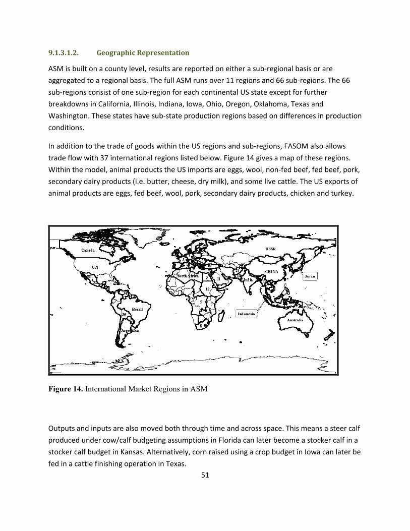
51

9.1.3.1.2. Geographic Representation

ASM is built on a county level, results are reported on either a sub-regional basis or are

aggregated to a regional basis. The full ASM runs over 11 regions and 66 sub-regions. The 66

sub-regions consist of one sub-region for each continental US state except for further

breakdowns in California, Illinois, Indiana, Iowa, Ohio, Oregon, Oklahoma, Texas and

Washington. These states have sub-state production regions based on differences in production

conditions.

In addition to the trade of goods within the US regions and sub-regions, FASOM also allows

trade flow with 37 international regions listed below. Figure 14 gives a map of these regions.

Within the model, animal products the US imports are eggs, wool, non-fed beef, fed beef, pork,

secondary dairy products (i.e. butter, cheese, dry milk), and some live cattle. The US exports of

animal products are eggs, fed beef, wool, pork, secondary dairy products, chicken and turkey.

Figure 14. International Market Regions in ASM

Outputs and inputs are also moved both through time and across space. This means a steer calf

produced under cow/calf budgeting assumptions in Florida can later become a stocker calf in a

stocker calf budget in Kansas. Alternatively, corn raised using a crop budget in Iowa can later be

fed in a cattle finishing operation in Texas.

52

Land allocations for livestock operations are assigned based on the biological carrying capacity

of land in a particular region. Each animal in a cow/calf or grazing operation requires a certain

amount of animal months of grazing from pasture land according to the budgets within FASOM

specific to a particular sub-region. Similarly, feedlots are assigned a specific amount of land to

operate. ASM can shift land from pasture land to crop land, indicating a movement from animal

production to crop production or vice versa.

9.1.3.1.3. Modeling the Market

The market structure in FASOM includes a mixture of explicit and implicit demand and supply

curves in a five-year period that are solved such that the affected agricultural markets are in

equilibrium (Adams et al.). In the case of animal disease, land cannot shift to reach equilibrium

but as supplies change in response to the slaughter price will shift. From Adams et al. these

supply and demand curves include:

• regional product supply,

• national raw product demand,

• regional or national processed commodity demand,

• regional or national supply of processed commodities,

• regional or national (depending on commodity) export demand

• regional or national (depending on commodity) import supply,

• regional feed supply and demand,

• regional direct livestock demand,

• international transport perfectly elastic supply and

• country-specific excess demand and supply of rice, sorghum, corn, soybeans and the 5

types of wheat

9.1.3.1.4. Using FASOM to Model Animal Disease

FASOM has several benefits in this type of analysis. First, it provides a great deal of detail in the

effects of a disease outbreak. In animal disease modeling there is an immediate death loss, but

there is also a reduction in the animals entering the meat chain in later periods due to the need

to replace breeding stock. For example, in beef cattle, heifers that would have been fed out are

instead diverted to replacement breeding stock. This more fully captures, not just the one shot

death loss of the disease, but also the long term recovery of the industry from the disease.

53

The regional structure also allows more detail since a disease shock can be confined

(quarantined) to a single region or sub-region and system resilience can be reflected with

readjustments in the locus of production. Also inputs like feed are diverted to alternative

beneficial uses. The FASOM model also captures the change in welfare from an animal disease

because it calculates a dollar loss of value added net income and a cost of commodity prices

rising. The trade impacts can also be estimated within FASOM.

Impact of Foot-and -Mouth Disease Management...

Documents

Transcript of Impact of Foot-and -Mouth Disease Management...