Impact of Channel Width on the Performance

of Long-distance 802.11 Wireless Links

Jhair Tocancipa TrianaT

HE

U N I V E RS

IT

Y

OF

ED I N B U

RG

H

Master of Science

Computer Science

School of Informatics

University of Edinburgh

2009

Abstract

A wireless communication channel can be characterized by a center of frequency (Fc)

and a channel width (Fw). Recent studies suggest that, in the presence of changing

environmental conditions, adjusting the channel width of a communication channel

might improve network variables like throughput and power consumption.

This thesis focuses on the effect that variable channel widths may have on the per-

formance of long distance IEEE 802.11 mesh networks, in particular on the Tegola net-

work, a network deployed at the Scottish Highlands by researchers from the University

of Edinburgh. One of the main contributions of this work is towards the understanding

of how variable channel widths could be used to improve the performance of wireless

long distance links affected by tidal effects.

i

Acknowledgements

I want to thank Prof. Mahesh Marina, head of the Wireless and Mobility Group (WiMo)

at the University of Edinburgh, for his continuous support during this project. I also

would like to thank Arsham Farshad and Sofia Pediaditaki, researchers from the WiMo

group, for their valuable feedback. Finally, I would like to express my gratitude to Prof.

Peter Buneman, Prof. Rick Rohde and Giacomo Bernardi for their assistance in setting

up a new long-distance wireless link for the Tegola network in the Scottish Highlands.

ii

Declaration

I declare that this thesis was composed by myself, that the work contained herein is

my own except where explicitly stated otherwise in the text, and that this work has not

been submitted for any other degree or professional qualification except as specified.

(Jhair Tocancipa Triana)

iii

Table of Contents

1 Introduction 1

2 Background and related work 32.1 Long-distance wireless mesh networks . . . . . . . . . . . . . . . . . 3

2.2 Link characteristics . . . . . . . . . . . . . . . . . . . . . . . . . . . 4

2.3 Interference characteristics . . . . . . . . . . . . . . . . . . . . . . . 5

2.4 The problem of channel width adaptation . . . . . . . . . . . . . . . 5

2.5 Medium Access Control (MAC) protocols . . . . . . . . . . . . . . . 6

2.6 Channel allocation . . . . . . . . . . . . . . . . . . . . . . . . . . . 8

3 Long-distance wireless link characteristics in the presence of tides 93.1 Simulation of the effect of tide levels on signal strength . . . . . . . . 10

3.2 Use of diversity to overcome the negative effect of tides on signal strength 11

4 Experimental study of the impact of channel width on network perfor-mance 144.1 Hardware and software . . . . . . . . . . . . . . . . . . . . . . . . . 14

4.2 Indoor experiments . . . . . . . . . . . . . . . . . . . . . . . . . . . 17

4.2.1 UDP throughput and packet loss at the receiver node . . . . . 19

4.2.2 Additional indoor investigations . . . . . . . . . . . . . . . . 20

5 Mitigating over water propagation effects using channel width adaptation 255.1 Preliminary activities . . . . . . . . . . . . . . . . . . . . . . . . . . 25

5.2 Issues faced after preliminary activities . . . . . . . . . . . . . . . . . 26

5.2.1 Low signal strength on the new test link . . . . . . . . . . . . 26

5.2.2 Production performance regression . . . . . . . . . . . . . . 27

5.2.3 Operating system crashes . . . . . . . . . . . . . . . . . . . . 28

5.3 Experimental results . . . . . . . . . . . . . . . . . . . . . . . . . . 28

iv

5.3.1 Tide levels affect the signal strength . . . . . . . . . . . . . . 29

5.3.2 The role of channel width adaptation . . . . . . . . . . . . . . 30

6 Conclusions and future work 34

A Basic concepts 36A.1 Signals . . . . . . . . . . . . . . . . . . . . . . . . . . . . . . . . . . 36

A.2 Channel characterization . . . . . . . . . . . . . . . . . . . . . . . . 37

B Link planning with SPLAT 38

C Greedy edge coloring implementation 41

Bibliography 44

v

Chapter 1

Introduction

In recent years, wireless mesh networks with long-distance point-to-point links have

shown to be a feasible, cost-effective alternative for broadband Internet access in rural

areas. Using commodity IEEE 802.11 equipment 1 and directional antennas it’s possi-

ble to build operational IP based mesh networks with link lengths in the order of tens

of kilometers. An example of such network is the Tegola network[1] deployed in the

Scottish Highlands by a team of the University of Edinburgh.

Although cost-effective, the use of IEEE 802.11 equipment to build long-distance

networks has some disadvantages. The protocols implemented by such equipment

were initially designed as an alternative to Ethernet-based LANs but not optimized

for long-distance links. For example, the use of channel reservation schemes such

as the Request to Send (RTS) and Clear to Send (CTS) exchange slows down the

performance long distance links, since the channels are usually allocated in such a way

that interference among adjacent links is avoided.

Efforts have been made by the research community to develop adaptive protocols

that work efficiently on long-distance networks. The basic idea behind adaptive pro-

tocols is to adjust some variable relevant to the network to improve its performance.

This adjustment can be done statically before deploying the network, or dynamically

adjusting the variable over time based on other parameters of the network, e.g. user

demand or environmental changes.

One variable of interest for adaptation is the center of frequency of the communica-

tion channels in the network. The range of frequencies passed by a given communica-

tion channel can be thought as centered around a particular frequency Fc. Algorithms

1Examples of this equipment includes radio cards and the software driver that controls them, bothimplementing the IEEE 802.11a standard.

1

Chapter 1. Introduction 2

have been devised by the research community to allocate centers of frequency in such

a way that the network throughput on long-distance links is improved. An instance of

such algorithm is presented by Dutta[2].

A relatively new idea is to adapt, in addition to Fc, the channel width Fw. Re-

cent research efforts by Chandra[3] focus on channel width adaptation on single links,

claiming throughput gains, in the presence of interference, up to 60% over static chan-

nel width allocation. Gummadi[4] studies how channel width adaptation among a set

of long-distance links can be used to reduce interference between the links.

Nevertheless, no known efforts have been made to study the effects of variable

channel widths on long distance wireless links over water. One of the contributions of

this thesis is to evaluate the feasibility of channel width adaptation as a mechanism to

counter the negative effect of variable tide levels.

The structure of this thesis is as follows. Chapter 2 provides some background on

long-distance wireless networks and channel (width) allocation. Chapter 3 discusses

the simulation of several diversity mechanisms in the presence of tidal effects. Chapter

4 focuses on the hardware/software requirements to evaluate variable channel widths,

and provides indoor experimental results. Chapter 5 describes the changes done to the

Tegola network to get nodes with variable channel width support, and analyzes outdoor

experimental results. Finally, Chapter 6 contains the conclusions and outlines venues

of future work.

Chapter 2

Background and related work

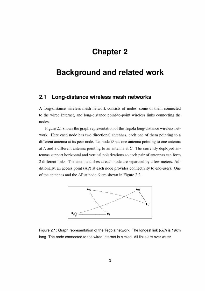
2.1 Long-distance wireless mesh networks

A long-distance wireless mesh network consists of nodes, some of them connected

to the wired Internet, and long-distance point-to-point wireless links connecting the

nodes.

Figure 2.1 shows the graph representation of the Tegola long-distance wireless net-

work. Here each node has two directional antennas, each one of them pointing to a

different antenna at its peer node. I.e. node O has one antenna pointing to one antenna

at I, and a different antenna pointing to an antenna at C. The currently deployed an-

tennas support horizontal and vertical polarizations so each pair of antennas can form

2 different links. The antenna dishes at each node are separated by a few meters. Ad-

ditionally, an access point (AP) at each node provides connectivity to end-users. One

of the antennas and the AP at node O are shown in Figure 2.2.

•G© •I

•O •B

•C

Figure 2.1: Graph representation of the Tegola network. The longest link (GB) is 19km

long. The node connected to the wired Internet is circled. All links are over water.

3

Chapter 2. Background and related work 4

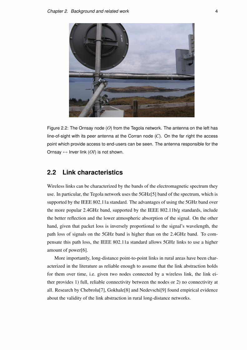
Figure 2.2: The Ornsay node (O) from the Tegola network. The antenna on the left has

line-of-sight with its peer antenna at the Corran node (C). On the far right the access

point which provide access to end-users can be seen. The antenna responsible for the

Ornsay↔ Inver link (OI) is not shown.

2.2 Link characteristics

Wireless links can be characterized by the bands of the electromagnetic spectrum they

use. In particular, the Tegola network uses the 5GHz[5] band of the spectrum, which is

supported by the IEEE 802.11a standard. The advantages of using the 5GHz band over

the more popular 2.4GHz band, supported by the IEEE 802.11b/g standards, include

the better reflection and the lower atmospheric absorption of the signal. On the other

hand, given that packet loss is inversely proportional to the signal’s wavelength, the

path loss of signals on the 5GHz band is higher than on the 2.4GHz band. To com-

pensate this path loss, the IEEE 802.11a standard allows 5GHz links to use a higher

amount of power[6].

More importantly, long-distance point-to-point links in rural areas have been char-

acterized in the literature as reliable enough to assume that the link abstraction holds

for them over time, i.e. given two nodes connected by a wireless link, the link ei-

ther provides 1) full, reliable connectivity between the nodes or 2) no connectivity at

all. Research by Chebrolu[7], Gokhale[8] and Nedevschi[9] found empirical evidence

about the validity of the link abstraction in rural long-distance networks.

Chapter 2. Background and related work 5

2.3 Interference characteristics

Phenomena such as multi-path, external interference, propagation delay and path loss

directly affect the performance of long-distance wireless links. Nevdevschi[9] pro-

vides evidence on how interference due to multi-path has little or no impact on the

performance of long-distance links. On the other hand, in the same research, a strong

correlation between the centers of frequency of adjacent links and packet loss rate is

found.

As mentioned in section 2.1 nodes in long-distance mesh networks have one direc-

tional antenna per link. Ireland[10] shows how the throughput on a given long-distance

link can vary significantly depending on antenna characteristics such as orientation,

placement and polarization.

A possible explanation for this variation is given by Raman[11]. Even with high

antenna gains, side-lobe radiation generated by antennas placed near each other, us-

ing the same center of frequency, will cause packet loss due to interference. Raman

found, empirically, that simultaneous transmission and reception at a given node cause

interference due to side-lobe radiation. E.g., in the graph shown in Figure 2.1, signals

being received at G from B and signals being transmitted from G to I simultaneously

interfere with each other, iff both links use the same channel. This interference is also

known as Mix-Rx-Tx interference1.

2.4 The problem of channel width adaptation

Adaptive algorithms adjust their run-time behavior depending on resource availability

over time. The adjustment is made towards optimizing the value of a given metric.

In particular, a channel width adaptation algorithm assigns widths Fw to the links in a

network based on a given network performance metric, such as consumed power at the

nodes or average throughput.

The assignment of Fw makes only sense in conjunction of the assignment of a

center of frequency Fc. For this reason the channel width adaptation problem can be

thought as the assignment of 〈Fc,Fw〉 pairs to links on a network. The assignment of

the 〈Fc,Fw〉 pairs may require a channel negotiation phase, which is described in 2.6.

1The scenarios where all antennas at a node are either transmitting (Syn-Tx) or receiving (Syn-Rx)also cause interference due to side-lobe radiation. However, Raman’s results suggest that the packet lossin the Syn-Rx and Syn-Tx cases is significantly lower than in the Mix-Rx-Tx case.

Chapter 2. Background and related work 6

Chandra[3] provides experimental evidence of the benefits of adjusting the chan-

nel width of a single link on a wireless LAN. A channel adaptation algorithm called

SampleWidth assigns a center of frequency Fw ∈ {5,10,20,40}MHz to a given link

based on the average throughput T and average data rate R measured on the link2,

aiming to maximize the throughput from the sender to the receiver. Chandra claims

that SampleWidth converges to the optimal channel width, i.e. to the Fw where the

throughput from the sender to the receiver is the highest.

Theoretical and experimental evidence of the benefits of channel width adaptation

in the context of long-distance urban links is provided by Gummadi[4]. The authors

present the channel adaptation algorithm VWID which assigns 〈Fc,Fw〉 pairs to links

on a network. VWID is somewhat similar to SampleWidth since it also uses probes

to measure the throughput of a link, and based on those measurements, decide which

〈Fc,Fw〉 pair is optimal. However VWID takes into account the throughput of several

links simultaneously while SampleWidth focuses on a single link only.

VWID is not distributed, i.e. the assignment of channel widths is done by a central-

ized entity which has knowledge about the global state of the network. Unfortunately,

Gummadi doesn’t provide details about their strategy to ensure that two end-points of

a given link are assigned the same 〈Fc,Fw〉 pair.

2.5 Medium Access Control (MAC) protocols

The consensus in the research community is that the IEEE 802.11 MAC protocols

are ill-suited for long-distance links. The higher propagation delays in long-distance

links imply that retransmissions are more frequent due to ACK packets received af-

ter the ACK timeout3. With the CSMA/CA4 protocol, the probability that two nodes

sense the medium as idle and send frames to reserve the medium simultaneously, caus-

ing a collision, increases with the distance between nodes. Moreover, as shown by

Gummadi[4], CSMA/CA imposes a non-optimal theoretical upper bound to the aggre-

gated throughput.

2Here an informal description of the algorithm: In a probing step the algorithm measures T and Rand compares R with constant data rates α and β. If R is lower than α, a lower Fw value is set for thelink. If R is greater than β, a higher Fw value is set for the link. The probing step is then performedagain with the new chosen Fw (the number of probes is finite). Once all probes terminate, the algorithmassigns Fw the channel width for which the measured throughput from the sender to the receiver was thehighest.

3For this reason, long-distance networks like Tegola need to adjust the ACK timeout to avoid suchretransmissions.

4Carrier Sense Multiple Access/Collision Avoidance.

Chapter 2. Background and related work 7

Examples of a MAC protocol proposed by the research community to overcome

some of the IEEE 802.11 MAC limitations are the P2P protocol and the JazzyMac

protocol[12].

The P2P protocol designed by Raman[11] aims to be an efficient alternative to

CSMA/CA, allowing maximum throughput even if adjacent links in the network use

the same center of frequency.

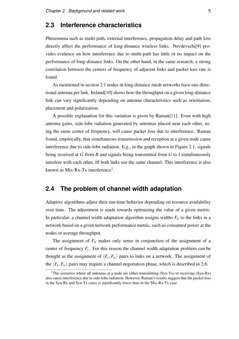
To see how P2P works, consider the bipartite graph shown in Figure 2.3. Let V1

be the set of nodes in the first partition and V2 the set of nodes in the second partition.

With P2P, during time slot t, the nodes in V1 = {O,G} transmit (nodes are in Tx mode)

while the nodes in V2 = {I,B,C} listen (nodes are in Rx mode).

•G •I

•O •B

•C

〈Fc,Fw〉

))〈Fc,Fw〉

""

〈Fc,Fw〉

77

〈Fc,Fw〉//

Figure 2.3: P2P nodes from the first partition in Tx mode.

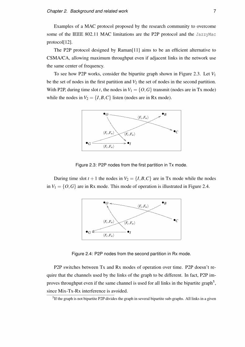
During time slot t + 1 the nodes in V2 = {I,B,C} are in Tx mode while the nodes

in V1 = {O,G} are in Rx mode. This mode of operation is illustrated in Figure 2.4.

•G •I

•O •B

•C

mm〈Fc,Fw〉WW

〈Fc,Fw〉

ss

〈Fc,Fw〉

oo〈Fc,Fw〉

Figure 2.4: P2P nodes from the second partition in Rx mode.

P2P switches between Tx and Rx modes of operation over time. P2P doesn’t re-

quire that the channels used by the links of the graph to be different. In fact, P2P im-

proves throughput even if the same channel is used for all links in the bipartite graph5,

since Mix-Tx-Rx interference is avoided.5If the graph is not bipartite P2P divides the graph in several bipartite sub-graphs. All links in a given

Chapter 2. Background and related work 8

2.6 Channel allocation

While the protocols presented in the section 2.5 try to improve throughput under the

assumption that all links use the same center of frequency (or channel), another fam-

ily of protocols exists that allocates different centers of frequency to adjacent links,

effectively avoiding packet loss due to Mix-Rx-Tx interference.

Dutta[2] proposes an algorithm based on graph coloring that assigns a different Fc

to every link at a given node in such a way that no two adjacent links get the same

center of frequency. Given that Mix-Rx-Tx interference is only relevant for links using

the same center of frequency, the application of the Dutta’s algorithm improves the

throughput of each link in a network. Nevertheless, the algorithm is static, i.e. it’s run

over a network topology without taking into account traffic, routing or other dynamic

aspects of the network.

As an additional contribution of this thesis, an implementation of a greedy graph

coloring algorithm is presented in Appendix C.

Instead of assigning centers of frequency at network design time, they could be

assigned in real-time. Wormsbecker[13] suggests the introduction of a channel nego-

tiation phase where the end-points of a given link agree on the Fc to use. A simple

protocol for this would involve one end-point sending a list of available frequencies

(channels) to its peer. This peer would select one of the received frequencies and use

it to start data transmission. This could be done with a new protocol or, as Worms-

becker proposes, extending the IEEE 802.11 MAC’s RTS/CTS frames with a bit-mask

representing the different Fc values being negotiated.

A channel width negotiation algorithm, at the application level, used to perform the

automatized measurements for this project is presented in Section 4.2.

sub-graph is assigned the same channel. Adjacent sub-graphs get assigned different channels. Then thesynchronized Rx-Tx modes are executed on each sub-graph.

Chapter 3

Long-distance wireless link

characteristics in the presence of tides

The long-distance links of the Tegola network are not as stable as expected by previous

research (see Section 2.2), which didn’t focus on over water signal propagation. For

instance, Bernardi[1] documents significant fluctuations in the Sound to Noise (SNR)

ratio and Received Signal Strength Indication (RSSI) measured at the Tegola nodes,

as much as 20dB over 1-2 hour periods. Bernardi suggest that a major cause of such

fluctuations might be the changes in the sea levels caused by the tidal effect. Recent

measurements by G. Bernardi showing these fluctuations are shown in Figure 3.1.

16

18

20

22

24

26

28

30

32

34

06/0300:00

06/0304:00

06/0308:00

06/0312:00

06/0316:00

06/0320:00

06/0400:00

SN

R(d

B)

Time

SNR for the Beinn to CollegeN link

ath0 (V polarization)ath2 (H polarization)

-78

-76

-74

-72

-70

-68

-66

-64

-62

-60

-58

06/0300:00

06/0304:00

06/0308:00

06/0312:00

06/0316:00

06/0320:00

06/0400:00

RS

SI(

dBm

)

Time

RSSI for the Beinn to CollegeN link

ath0 (V polarization)ath2 (H polarization)

Figure 3.1: Fluctuations of SNR (left) and RSSI (right) over a 24 hours period on the

Beinn↔ College link. This is the GB link shown in Figure 2.1.

To better understand the relationship between tidal effects and signal strength soft-

ware simulations were performed.

9

Chapter 3. Long-distance wireless link characteristics in the presence of tides 10

3.1 Simulation of the effect of tide levels on signal strength

The Corran↔ Ornsay long-distance link 1 was modeled with the third-party software

Pathloss2. Pathloss is an advanced package for the simulation and analysis of several

wireless phenomena, such as refraction, reflection and multipath. For the simulation

of tidal effects the reflection module was used.

The inputs of the simulation include:

1. Node information: This includes the geographical coordinates of the nodes to-

gether with the channel frequencies and antenna gains.

2. Elevation pattern: Based on the node information and its terrain database, Pathloss

generates the elevation pattern between both nodes. The obtained elevation pat-

tern is shown Figure 3.2.

Figure 3.2: Elevation pattern generated by Pathloss (left) and antenna height

settings (right) for the Corran↔ Ornsay link.

3. Antenna heights. These were set at 2m for the Ornsay node and at 3m for the

Corran node. The line-of-sight is shown in Figure 3.2.

4. Reflective plane. A constant elevation (0m) reflective plane at sea level was

defined. This reflective plane is shown in Figure 3.3.

5. Channel frequencies, polarization (vertical) and tidal level range ([1 . . .5]m).

With the provided inputs Pathloss calculates the relative signal strength for the

different tide levels. The results of this calculation are shown in Figure 3.3. Here,

1This is the OC link shown in Figure 2.1.2http://www.pathloss.com/

Chapter 3. Long-distance wireless link characteristics in the presence of tides 11

Figure 3.3: Sea level reflection plane (left) and simulation results showing the

effect of the tide level on signal strength (right).

when the tide level is 2.5m high the lowest signal strength is expected. This lowest

point is also known in the literature as a null. On the other hand, tide levels above the

2.5m should increase the signal strength for the given polarization, antenna height and

radio frequency.

3.2 Use of diversity to overcome the negative effect of

tides on signal strength

Diversity techniques are commonly used to reduce the effect of environmental phe-

nomena (e.g. tide levels) on the quality of a wireless link. Three forms of diversity for

the Corran↔ Ornsay link were simulated with Pathloss:

• Frequency diversity: In this case the nodes adjust the center of frequency in such

a way that the signal strength is maximized. This is illustrated in Figure 3.4

(bottom right). Here, when the tide is 2.5m high, channel 36(5.18GHz) provides

the lowest signal strength. Switching to the channel 165(5.825GHz) improves

the signal strength at the 2.5m tide level, all other things being equal.

• Polarization diversity: Here the polarization that improves the signal strength

is preferred. Pathloss predicts a slightly better signal strength when using the

vertical polarization. This is shown in Figure 3.4 (bottom left).

• Antenna height diversity: In this case, at a given node, a second antenna is placed

at a height d with respect to the original antenna. d is chosen in such a way

that the null signal strength value obtained with the original antenna becomes

Chapter 3. Long-distance wireless link characteristics in the presence of tides 12

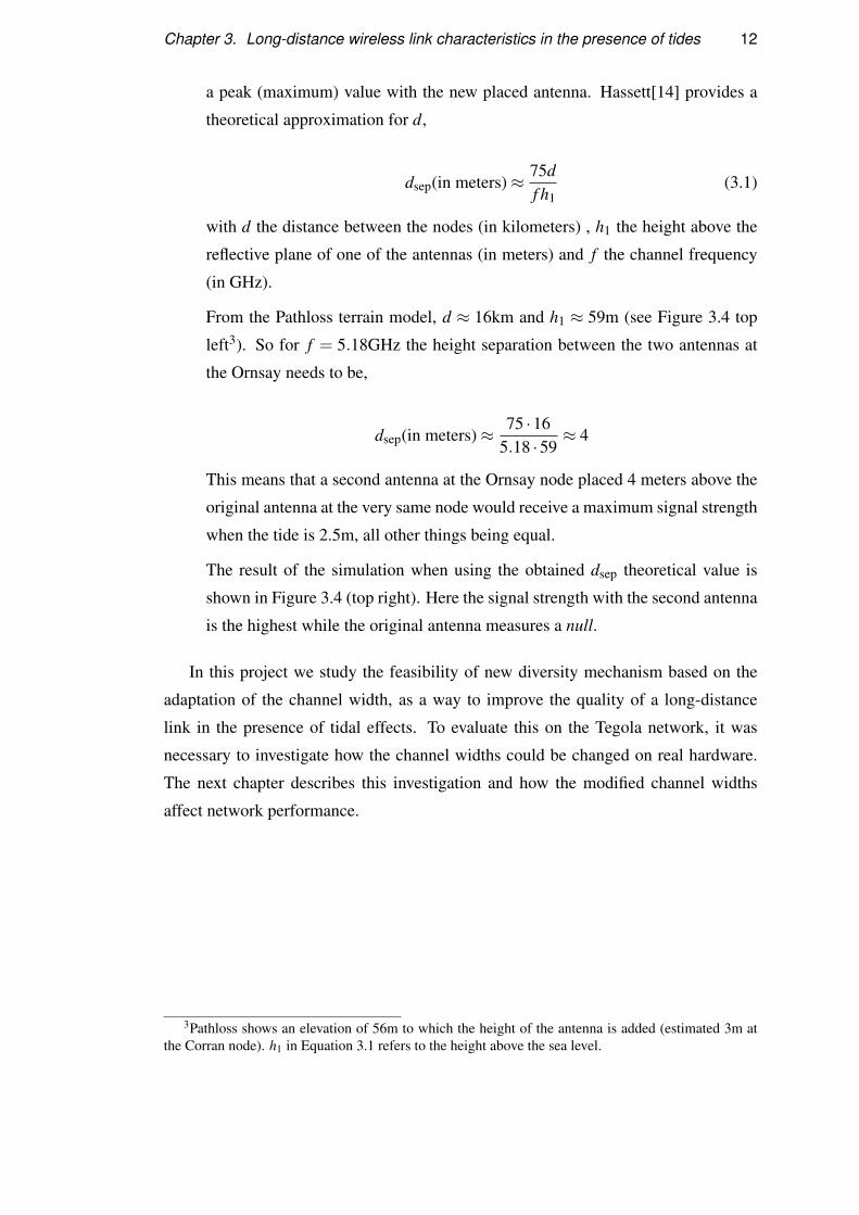
a peak (maximum) value with the new placed antenna. Hassett[14] provides a

theoretical approximation for d,

dsep(in meters)≈ 75df h1

(3.1)

with d the distance between the nodes (in kilometers) , h1 the height above the

reflective plane of one of the antennas (in meters) and f the channel frequency

(in GHz).

From the Pathloss terrain model, d ≈ 16km and h1 ≈ 59m (see Figure 3.4 top

left3). So for f = 5.18GHz the height separation between the two antennas at

the Ornsay needs to be,

dsep(in meters)≈ 75 ·165.18 ·59

≈ 4

This means that a second antenna at the Ornsay node placed 4 meters above the

original antenna at the very same node would receive a maximum signal strength

when the tide is 2.5m, all other things being equal.

The result of the simulation when using the obtained dsep theoretical value is

shown in Figure 3.4 (top right). Here the signal strength with the second antenna

is the highest while the original antenna measures a null.

In this project we study the feasibility of new diversity mechanism based on the

adaptation of the channel width, as a way to improve the quality of a long-distance

link in the presence of tidal effects. To evaluate this on the Tegola network, it was

necessary to investigate how the channel widths could be changed on real hardware.

The next chapter describes this investigation and how the modified channel widths

affect network performance.

3Pathloss shows an elevation of 56m to which the height of the antenna is added (estimated 3m atthe Corran node). h1 in Equation 3.1 refers to the height above the sea level.

Chapter 3. Long-distance wireless link characteristics in the presence of tides 13

Figure 3.4: Pathloss simulation results for antenna height diversity (top right), polar-

ization diversity (bottom left) and frequency diversity (bottom right). The geographical

information entered in Pathloss for the Corran↔ Ornsay link is shown at the top left.

Chapter 4

Experimental study of the impact of

channel width on network

performance

Variable channel widths require hardware and software support. For this project, hard-

ware (radio cards) supporting variable channel widths were made available by the

WiMo group. These are the same type of cards being used at the nodes of the Tegola

network.

On the other hand, the software currently running on those cards didn’t support

variable channel widths. For this reason, the software on the cards needed to be up-

graded. Since the cards are embedded devices, efforts were made to learn the skills

required for embedded software installation and development. This learning effort

was facilitated by the Tegola network’s documentation1.

4.1 Hardware and software

The hardware involved in the experiments included:

• Gateworks Avila GW2348-4 boards: these are embedded devices controlled by

an Intel IXP425 processor (ARM architecture). The boards have 15Mb of flash

memory, 64Mb of SDRAM, two Ethernet ports and a serial RS-232 interface.

Four 32-bit mini-PCI Type III sockets are also provided. The boards are powered

by a 9-48V@23W interface.

1http://www.tegola.org.uk/dev/index.php/Main_Page

14

Chapter 4. Experimental study of the impact of channel width on network performance15

• Ubiquiti Networks XtremeRange5 radio cards: these are 32-bit mini-PCI Type

III cards which can be installed on the PCI sockets of the Gateworks Avila

boards. These cards provide a single MMCX antenna port. The cards are based

on the Atheros AR5414 radio-on-a-chip (RoC) which supports the IEEE 802.11a

standard. Support for 5, 10, 20 and 40MHz channel widths is provided.

• Pigtails: These are the cables used to connect an antenna to the MMCX port on

the radio cards.

• Laird 5.8GHz omnidirectional antennas: These are antennas with 3dBi power

gain. Were used in the indoor experiments.

• Directional Laird HDDA5W-29-DP dish antennas: These are antennas with 29dBi

power gain and dual polarization used for the long-distance links on the Tegola

network.

• Directional 5.8GHz parabolic grid antennas: These are antennas with 30dBi gain

used to create a new outdoor test link described in section 5.1.

• Wi-Spy USB 5GHz spectrum analyzer: this device is used to track the amplitude

and width of the signals traveling through the air during the experiments. It was

particularly valuable for debugging purposes.

The software compiled and installed by the author to control the hardware included:

• OpenWrt 8.09.1 (Kamikaze) GNU/Linux operating system: this operating sys-

tem is aimed at embedded devices. This version is based on the 2.6.26.8 release

of the Linux kernel and supports the Intel IXP425 processor found in the Gate-

works Avila boards. It also includes the free Madwifi driver, release version

0.9.4, for Atheros based cards (such as the XtremeRange5 radio cards).

• Ubiquiti Networks 0.7-beta.379 driver for the XtremeRange5 radio cards: this

driver is based on the free Madwifi driver, development version r3319 from the

Subversion repository2.

• spectools utilities: these are applications for the Wi-Spy USB 5GHz spectrum

analyzer. The development version r3319 from the Subversion repository3 was

used. The tool was installed on a laptop running Ubuntu 8.04.1 GNU/Linux.2http://svn.madwifi-project.org/madwifi/trunk3https://www.kismetwireless.net/code/svn/tools/spectools

Chapter 4. Experimental study of the impact of channel width on network performance16

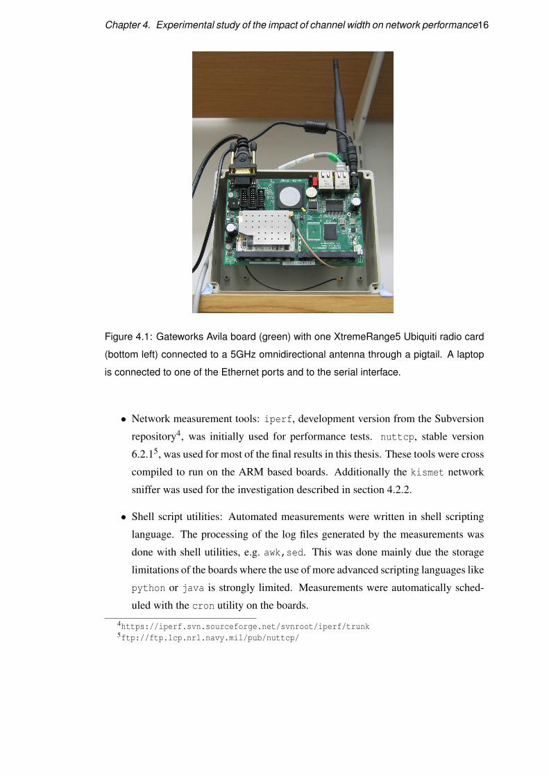
Figure 4.1: Gateworks Avila board (green) with one XtremeRange5 Ubiquiti radio card

(bottom left) connected to a 5GHz omnidirectional antenna through a pigtail. A laptop

is connected to one of the Ethernet ports and to the serial interface.

• Network measurement tools: iperf, development version from the Subversion

repository4, was initially used for performance tests. nuttcp, stable version

6.2.15, was used for most of the final results in this thesis. These tools were cross

compiled to run on the ARM based boards. Additionally the kismet network

sniffer was used for the investigation described in section 4.2.2.

• Shell script utilities: Automated measurements were written in shell scripting

language. The processing of the log files generated by the measurements was

done with shell utilities, e.g. awk,sed. This was done mainly due the storage

limitations of the boards where the use of more advanced scripting languages like

python or java is strongly limited. Measurements were automatically sched-

uled with the cron utility on the boards.

4https://iperf.svn.sourceforge.net/svnroot/iperf/trunk5ftp://ftp.lcp.nrl.navy.mil/pub/nuttcp/

Chapter 4. Experimental study of the impact of channel width on network performance17

4.2 Indoor experiments

The first goal was to evaluate the Ubiquiti driver to ensure that the variable channel

widths were being correctly set by the driver. The change of the channel widths is

controlled by values of a particular entry of the proc filesystem on the boards (with

the exception of the 40MHz width channel). Table 4.1 shows the required commands.

Channel width (MHz) Shell command

5 echo 0x156d0001 > /proc/sys/dev/wifiX/cwidth

10 echo 0x156d0002 > /proc/sys/dev/wifiX/cwidth

20 (default) echo 0x156d0000 > /proc/sys/dev/wifiX/cwidth

40 (TurboMode) iwpriv athX turbo 1

Table 4.1: Commands to change the channel width on interface X. Before issuing each

command the interface must be shut down (ifconfig athX down) and after each

command the interface must be activated (ifconfig athX up).

Two boards connected to omnidirectional antennas were configured to communi-

cate with each other in point-to-point (ad-hoc) mode. Both cards shared the same IEEE

802.11a channel, same channel widths and same IP subnetwork. Traffic was injected

to the wireless link with the nuttcp tool.

To avoid the influence of uncontrolled parameters in the final results some parame-

ters were set to particular values. For instance UDP was used to avoid the overhead of

transport layer (TCP) mechanisms, such as the Automatic Repeat reQuest (ARQ) pro-

tocol and the congestion control algorithm. The MAC layer data rate was fixed instead

of using the Minstrel rate adaptation algorithm provided by default by the Ubiquiti

driver. Minstrel basically adjusts the sender’s MAC layer data rate (6, 9, 12, 18, 24,

36, 48 or 54Mbps) and modulation (BPSK, QPSK or QAM) using heuristics based

on the quality of the link. The transmission power was also fixed at 10dBm. The

parameters are summarized in Table 4.2.

Chapter 4. Experimental study of the impact of channel width on network performance18

Algorithm 11: procedure SYNCCHANNELWIDTH(〈Fc,Fw〉source, interface, target, stats)

2: 〈Fc,Fw〉source← estimateBestWidth(〈Fc,Fw〉source, interface, stats)

3: 〈Fc,Fw〉target← send(target, changeChannel, 〈Fc,Fw〉source) . Synchronous call

4: if 〈Fc,Fw〉target = 〈Fc,Fw〉source then . Target adjusted its interface as proposed

5: adjustInterface(interface, 〈Fc,Fw〉source)

6: radio and MAC stats log start(interface, stats)

7: injectTraffic(interface)

8: radio and MAC stats log end(interface)

9: end if10: end procedure

A channel width synchronization algorithm was implemented as a shell script run-

ning on the boards. Algorithm 1 shows the pseudo-code of the synchronization pro-

cedure. This algorithm assumes the existence of an additional channel (interface) for

message passing (e.g. at Step 3 of the algorithm).

While traffic was flowing through the wireless link the spectrum analyzer was used

to gather the range of frequencies used by the channel. As shown in Figure 4.2 the

width of range of frequencies is proportional to the channel width set on the driver.

-110

-100

-90

-80

-70

-60

-50

-40

5.765GHz (153)

Sig

nal s

tren

gth

(dB

m)

Frequency (Channel)

5MHz10MHz20MHz

-110

-100

-90

-80

-70

-60

-50

-40

5.76GHz (152)

Sig

nal s

tren

gth

(dB

m)

Frequency (Channel)

40MHz (Turbo Mode)

Figure 4.2: Signal strength (y-axis) and range of frequencies (x-axis) as reported by

the Wi-Spy USB 5GHz spectrum analyzer. Each line on the plot corresponds to the

measured signal strength during a network performance test with the nuttcp tool.

Once there was confidence that the Ubiquiti driver was correctly limiting the range

of frequencies as the channel width changed, performance tests were done to evaluate

different network metrics.

Chapter 4. Experimental study of the impact of channel width on network performance19

Name Value

Transmitter node A (IP 192.168.3.11)

Receiver node B (IP 192.168.3.13)

Traffic type UDP

Measurement tool nuttcp

Transmission power 10dBm (fixed)

Data rate (MAC layer) 6Mbps (fixed)

Channels (center frequency) 152 (5.76GHz), 153 (5.765GHz)

RTS/CTS disabled

MAC layer ACKs enabled

Packet size 1490bytes

Test duration 20sec

Antenna Omnidirectional (3dBi gain)

Test frequency Per minute (scheduled with cron)

Table 4.2: General parameters for the indoor experiment on the wireless testbed at the

WiMo group’s laboratory (Informatics Forum).

4.2.1 UDP throughput and packet loss at the receiver node

A correlation between the channel width and the measured throughput at the server is

expected. From the Shannon capacity formula,

C = B log2(1+SNR) (4.1)

with C the capacity of the channel, B the bandwidth (or channel width) of the

channel in Hertz and the SNR (understood as the ratio between the signal and the

noise powers). Assuming a SNRdB = 20 (SNR = 102)6,

C40MHz = 40 ·106 · log2(1+102) ≈ 40 ·106 ·7 = 280Mbps

C20MHz ≈ 20 ·106 ·7 = 140Mbps

C10MHz ≈ 10 ·106 ·7 = 70Mbps

C5MHz ≈ 5 ·106 ·7 = 35Mbps

6SNRdB = 10log10(SNR) =⇒ SNR = 10SNRdB

10

Chapter 4. Experimental study of the impact of channel width on network performance20

I.e. by doubling the channel width we should expect an increase in the throughput

by a factor of two. Nevertheless the above rates cannot be achieved by IEEE 802.11

systems, given that the capacity formula provides only a theoretical upper bound re-

gardless the protocol used to transmit the data.

Jun[15] provides formulas for the estimation of the maximum theoretical through-

put expected by applications running over the IEEE 802.11 MAC layer. From Jun’s

formulas, the maximum expected throughput for a fixed 6Mbps OFDM modulation

with RTS/CTS frames disabled (as in the experiment (see Table 4.2)) should be near

the 5Mbps. Nevertheless, Figure 4.3 shows throughput in the order of 10Mbps with

the standard channel width of 20MHz.

The root cause of this discrepancy is the channel initially used for the experiment.

Channel 152 (and channels 50, 58, 152 and 160) support TurboMode (40MHz) width

channels. During the measurements the TurboMode was being activated by the driver

hence the increased measured throughput. For this reason, experiments with and with-

out 40MHz width channels needed to be performed separately.

The results of such indoor experiments are shown in Figure 4.4. A shell script

was written to loop over different rates and channel widths while running Algorithm

1. Here the doubling of the measured throughput as predicted by the capacity formula

can be observed for almost all rates. For the 40MHz channel width this trend could not

be observed for MAC layer transmission rates higher than 36Mbps. This result can not

be attributed to packet loss since the packet loss TurboMode was less than the packet

loss for the 20MHz channel width.

The obtained results, for the 5, 10 and 20MHz channel widths, reproduced previous

results from Chandra[3] where the effect of channel widths on throughput in indoor

environments was first studied. This gave confidence in moving forwards to perform

the necessary activities to make measurements with variable channel widths on the

Tegola network itself.

4.2.2 Additional indoor investigations

To further reduce the number of uncontrolled parameters during the experiments an in-

vestigation was performed to find out how to deactivate the sending of MAC layer ac-

knowledgments at the target node. Due the greater probability of packet loss in wireless

networks over wired networks, the IEEE 802.11 MAC layer provides an ARQ mecha-

nism for data reliability. When measuring the effect of channel widths on throughput

Chapter 4. Experimental study of the impact of channel width on network performance21

0

2

4

6

8

10

12

04:00 06:00 08:00 10:00 12:00 14:00 16:00

Thr

ough

put -

Nod

e B

(M

bps)

Time (hour)

20MHz10MHz5MHz

0

500

1000

1500

2000

2500

3000

3500

4000

4500

04:00 06:00 08:00 10:00 12:00 14:00 16:00

UD

P p

acke

ts lo

st

Time (hour)

20MHz10MHz5MHz

Figure 4.3: Measured throughput at the receiver (left) and UDP packet loss (right) for

different channel widths.

these acknowledgments might also be an overhead in the same way ARQ mechanisms

provided by TCP are.

The Ubiquiti and Madwifi drivers don’t provide a parameter to deactivate the MAC

layer acknowledgments. Fortunately the source code of the drivers is freely available

and the deactivation of MAC layer acknowledgments was already done by members of

the Madwifi user community. Disabling acknowledgments requires two basic changes:

1. Disable the automatic generation of acknowledgments by the hardware of the

receiver node. This is done by writing a particular value to a hardware register

of the radio card, e.g. with:

OS_REG_WRITE(ah, 0x8048, 0x00000002);

2. Tell the hardware don’t to wait for acknowledgments before transmitting data.

This is done by passing a particular flag to the HAL:

flags |= HAL_TXDESC_NOACK;

Both changes and the rationale behind it were already available in the mailing list

of the Madwifi driver7. The changes were ported to the Ubiquiti driver by the author

and by Arsham Farshad and then made available in a git version control repository

for better interaction with other researchers at the WiMo group 8.

7http://thread.gmane.org/gmane.linux.drivers.madwifi.devel/61608The repository is accessible with git clone git@github.com:jhairtt/ubnt-hal-0.7.379.git.

Chapter 4. Experimental study of the impact of channel width on network performance22

0

5

10

15

20

25

30

35

40

6 9 12 18 24 36 48 54

Thr

ough

put -

Nod

e B

(Mbp

s)

MAC layer data rate (Mbps)

5MHz10MHz20MHz40MHz

0

1

2

3

4

5

6

6 9 12 18 24 36 48 54

% P

acke

t Los

s

MAC layer data rate (Mbps)

20MHz40MHz

Figure 4.4: Throughput measured indoor for different modulations and channel widths.

The maximum 27dBm transmission power was used. The 40MHz channel width was

tested on channel 42. Other channel widths were tested on channel 149.

The modified driver was then cross compiled for the ARM architecture and in-

stalled on the boards. Additionally the kismet 802.11 network sniffer was installed on

the transmitter node and iperf UDP traffic was generated from this node. The tshark

utility was used to analyze the data gathered by kimset. For instance,

tshark -r "wlan.fc.type_subtype == 0x1d && \

wlan.ra == 00:15:6d:63:a1:d5" kismet_dump_file

reports the MAC layer acknowledgments originated from the network card with

MAC address 00:15:6d:63:a1:d5.

Because of time constraints the modified driver with disabled acknowledgments

was not used for the experiments described in this research. It has been used by other

researchers at the WiMo group though.

Chapter 4. Experimental study of the impact of channel width on network performance23

-120

-100

-80

-60

-40

-20

0

20

40

60

04:00 06:00 08:00 10:00 12:00 14:00 16:00

dBm

Time (Hour)

Link QualitySignal Level

Noise

-70

-65

-60

-55

-50

-45

04:00 06:00 08:00 10:00 12:00 14:00 16:00N

oise

- N

ode

B(d

Bm

)

Time (Hour)

20MHz10MHz5MHz

28

30

32

34

36

38

40

42

44

46

48

04:00 06:00 08:00 10:00 12:00 14:00 16:00

Link

Qua

lity

- N

ode

B(d

Bm

)

Time (Hour)

20MHz10MHz5MHz

-70

-65

-60

-55

-50

-45

04:00 06:00 08:00 10:00 12:00 14:00 16:00

Sig

nal S

tren

gth

- N

ode

B(d

Bm

)

Time (Hour)

20MHz10MHz5MHz

Figure 4.5: Measured link quality, signal level and noise on the target node (top left)

during the experiments. The same data filtered by channel width is shown in the other

three graphs.

Chapter 4. Experimental study of the impact of channel width on network performance24

0

100

200

300

400

500

0 15 30

Cou

nt

Time (sec)

MAC ACKs enabledMAC ACKs disabled

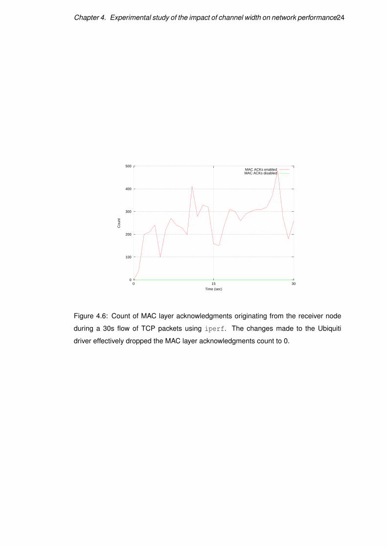
Figure 4.6: Count of MAC layer acknowledgments originating from the receiver node

during a 30s flow of TCP packets using iperf. The changes made to the Ubiquiti

driver effectively dropped the MAC layer acknowledgments count to 0.

Chapter 5

Mitigating over water propagation

effects using channel width adaptation

In order to evaluate the role of different channel widths on the Tegola network it was

decided to deploy a new long-distance test link and upgrade the software on some of

the nodes.

To achieve this goal, several preliminary activities were performed some of them

with the support from researchers at the WiMo group and Prof. Peter Buneman.

5.1 Preliminary activities

1. Test the two 5.8GHz parabolic grid antennas. They were tested indoor to confirm

their proper functioning before their deployment at the locations of the nodes of

the new test link.

2. Upgrade and configure the software of several Gateworks Avila boards. The

required software to allow variable channel widths, see section 4.1, was installed

and configured by the author on several boards at the WiMo group laboratory.

The installation and configuration of the OSPF routing software quagga1 was

performed by the researcher G. Bernardi at the location of each of the pertinent

nodes.

3. Replace boards on site and deploy a new test link. G. Bernardi, researcher from

the WiMo group, and the author visited the nodes at College, Corran and Ornsay

at the Isle of Skye (Scottish Highlands) to replace the Gateworks Avila boards1http://www.quagga.net/

25

Chapter 5. Mitigating over water propagation effects using channel width adaptation26

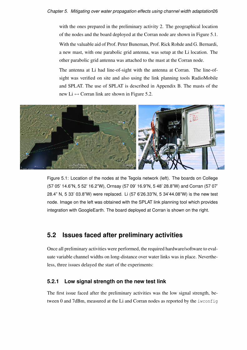
with the ones prepared in the preliminary activity 2. The geographical location

of the nodes and the board deployed at the Corran node are shown in Figure 5.1.

With the valuable aid of Prof. Peter Buneman, Prof. Rick Rohde and G. Bernardi,

a new mast, with one parabolic grid antenna, was setup at the Li location. The

other parabolic grid antenna was attached to the mast at the Corran node.

The antenna at Li had line-of-sight with the antenna at Corran. The line-of-

sight was verified on site and also using the link planning tools RadioMobile

and SPLAT. The use of SPLAT is described in Appendix B. The masts of the

new Li↔ Corran link are shown in Figure 5.2.

Figure 5.1: Location of the nodes at the Tegola network (left). The boards on College

(57 05’ 14.6”N, 5 52’ 16.2”W), Ornsay (57 09’ 16.9”N, 5 48’ 28.8”W) and Corran (57 07’

28.4” N, 5 33’ 03.8”W) were replaced. Li (57 6’26.33”N, 5 34’44.08”W) is the new test

node. Image on the left was obtained with the SPLAT link planning tool which provides

integration with GoogleEarth. The board deployed at Corran is shown on the right.

5.2 Issues faced after preliminary activities

Once all preliminary activities were performed, the required hardware/software to eval-

uate variable channel widths on long-distance over water links was in place. Neverthe-

less, three issues delayed the start of the experiments:

5.2.1 Low signal strength on the new test link

The first issue faced after the preliminary activities was the low signal strength, be-

tween 0 and 7dBm, measured at the Li and Corran nodes as reported by the iwconfig

Chapter 5. Mitigating over water propagation effects using channel width adaptation27

Figure 5.2: Parabolic grid antenna attached to the Corran mast (left) and mast with

parabolic grid antenna deployed at the Li node (right (Picture by G. Bernardi)). The

over water link has a length of 2.5km.

tool. Thanks to Prof. Buneman both nodes were visited twice by the autor and G.

Bernardi (which required two boat trips) to crosscheck the hardware.

Days later, Prof. Buneman himself replaced the radio cards at the Corran node

to discard them as the root cause of the problem. Additionally, the signal strength

was measured with the spectrum analyzer at Corran’s shore. Although signals were

detected by the spectrum analyzer, the signal strength was not enough to transmit data

with a high data rate to the Li node.

Tests done remotely from the WiMo laboratory demonstrated that ping packets

(and even ssh traffic) sent from one node could reach the other. However, the long

latencies made the execution of performance tests not possible. It’s highly probable

that the root cause is hardware related, e.g. cabling problems or a defective board.

Fortunately, since the boards at Ornsay and Corran were replaced, it was decided

to use the Ornsay↔ Corran link for the outdoor experiments. In order to avoid inter-

ference with user traffic, the vertical polarization of the link was used and all routing

(OSPF) traffic over the vertical polarized link disabled. These routing configuration

changes were done by G. Bernardi remotely from the WiMo laboratory.

5.2.2 Production performance regression

The second issue faced was a performance regression with the Ubiquiti driver. Pro-

duction users of the Tegola network complained about low throughput short after the

new boards were deployed. With G. Bernardi it was found that the root cause was the

SampleRate rate adaptation algorithm used by the driver. After instructing the driver

Chapter 5. Mitigating over water propagation effects using channel width adaptation28

to use the Minstrel rate adaptation algorithm the performance increased but wasn’t

completely satisfactory.

A possible reason for this might be the fact that the Ubiquiti driver predates the

original Madwifi driver so performance improvements made to the latest version of the

Madwifi driver are not available in the Ubiquiti driver. However the highest measured

throughput was good enough to run experiments (see Figure 5.3).

5.2.3 Operating system crashes

The third issue was crashes of the operating system on the boards, caused by the iperf

utility. Although iperf worked reliably on the boards during the indoor experiments,

any attempt to transmit data with this tool over the Corran ↔ Ornsay link resulted

on a crash (the same problem was experienced with netserver tool). A crash of the

operating system is a worst case scenario since the boards cannot be remotely reset.

During the visit to the Ornsay node one of the users was instructed on how to reset the

boards on site.

The only difference in the software configuration between the boards used for out-

door and indoor experiments was that the boards on Tegola run the routing software

(quagga). A tool with lower memory footprint than iperf, nuttcp2 worked reliably

without causing further crashes.

5.3 Experimental results

After the issues described in section 5.2 were solved, measurements were started on

the Ornsay↔ Corran link, most of them using the implementation of Algorithm 1.

First, the throughput for different modulations with the maximum transmission

power of 27dBm was obtained. The obtained results are shown in Figure 5.3. Here,

in TurboMode (40MHz channel width), the measured maximum throughput for the 6,

12 and 24Mbps data rates exceeds the theoretical value predicted by Jun[15]. For the

54Mpbs modulation the expected throughput is within bounds though.

The next experiment evaluated the throughput and the signal strenght at the nodes

when using a fixed 6Mbps transmission rate. The results of this experiment are shown

in Figure 5.4. Here the correlation between channel width and throughput described in

Section 4.2.1 is cleary seen.

2Which is implemented in a single .c file.

Chapter 5. Mitigating over water propagation effects using channel width adaptation29

0

5

10

15

20

25

30

35

40

6 12 24 54

Thr

ough

put (

Mbp

s)

MAC Layer data rate (Mbps)

Channel 42 (TurboMode)Channel 36

Figure 5.3: Maximum application level throughput on the Corran ↔ Ornsay link ob-

tained with 27dBm transmission power and different fixed MAC layer data rates.

From the Ubiquiti XtremeRange5 radio card’s technical specifications the card re-

ceiver sensitivity to achieve a 6Mbps rate is -94dBm. As seen in Figure 5.4 the signal

strength at Ornsay is in the order of -70dBm, above the sensitivity threshold for 6Mbps.

This explains the stable throughput for autorate in Figure 5.4, i.e. the link quality is

good enough to use the predetermined fixed rate.

5.3.1 Tide levels affect the signal strength

Comparing the obtained measuruments with the tide level information provided by

the BBC weather site3 some correlation between the tide level and the signal strength

was observed. For instance, in Figure 5.4 the highest tide level (4m) measured at

20:00 matches the highest signal strength on both end nodes of the link. This peak is

consistent with the Pathloss simulation results shown in Section 3.1 (channel frequency

5180MHz).

Although the peak signal strength and the highest tide level seem to happen simul-

taneously, this experiment cannot be regarded as a proof of a cause-effect relationship

between tide level and signal strength. There are several reasons for this:

3E.g. http://www.bbc.co.uk/weather/coast/tides/tides.shtml?date=20090811\&loc=0367 for the tide level at Corran on 2009-08-11.

Chapter 5. Mitigating over water propagation effects using channel width adaptation30

Name Value

Transmitter node Corran (IP 10.3.0.1)

Receiver node Ornsay (IP 10.1.0.25)

Traffic type UDP

Measurement tool nuttcp

Transmission power 10dBm (fixed)

Data rates (MAC layer) 6Mbps (fixed) and autorate (Minstrel algorithm)

Channels (center frequency) 36 (5.18GHz), 42 (5.22GHz)

RTS/CTS disabled

MAC layer ACKs enabled

Packet size 1490bytes

Test duration 20sec

Antenna Directional (29dBi gain)

Test frequency Per minute (scheduled with cron)

Table 5.1: General parameters for the outdoor experiment on the Tegola network.

1. Granularity of the tide level data: numerical data is provided every 6 hours, while

the radio statistics are gathered automatically every 2 minutes. That’s the reason

of the saw-toothed pattern in in Figure 5.4.

2. Clock synchronization: Although the clocks of all nodes in the Tegola network

are synchronized with the ntp protocol, there is no guarantee that the clocks

are synchronized with the BBC’s computers providing the tide level informa-

tion. This can yield to shifts between the measured radio statistics and the tide

information.

5.3.2 The role of channel width adaptation

To investigate how the variable channel widths might be used as a diversity mechanism

further measurements were done over several days. For this experiment the Minstrel

rate adaptation algorithm was used on the transmitter node (Corran).

The results of this experiment are shown in Figures 5.5 and 5.6. The fluctuations in

throughput when using the 20MHz channel width are consistent with the packet loss.

Again, the correlation between channel width and throughput described in Section

4.2.1 is observed.

Chapter 5. Mitigating over water propagation effects using channel width adaptation31

0

0.5

1

1.5

2

2.5

3

3.5

08/1115:00

08/1116:00

08/1117:00

08/1118:00

08/1119:00

08/1120:00

08/1121:00

08/1122:00

08/1123:00

08/1200:00

08/1201:00

08/1202:00

08/1203:00

Thr

ough

put (

Mbp

s)

Time (hour)

20MHz10MHz5MHz

-80

-78

-76

-74

-72

-70

-68

-66

-64

-62

-60

08/1115:00

08/1116:00

08/1117:00

08/1118:00

08/1119:00

08/1120:00

08/1121:00

08/1122:00

08/1123:00

08/1200:00

08/1201:00

08/1202:00

08/1203:00

Sig

nal S

tren

gth

- O

rnsa

y (d

Bm

)

Time (Hour)

20MHz10MHz5MHz

-95

-90

-85

-80

-75

-70

-65

-60

-55

-50

08/1115:00

08/1116:00

08/1117:00

08/1118:00

08/1119:00

08/1120:00

08/1121:00

08/1122:00

08/1123:00

08/1200:00

08/1201:00

08/1202:00

08/1203:00

Sig

nal S

tren

gth

- C

orra

n (d

Bm

)

Time (Hour)

20MHz10MHz5MHz

0

0.5

1

1.5

2

2.5

3

3.5

4

4.5

5

08/1116:00

08/1118:00

08/1120:00

08/1122:00

08/1200:00

08/1202:00

Tid

e Le

vel -

Cor

ran

(m)

Time (Hour)

Tide Level

Figure 5.4: Throughput, signal strength and tide level for an experiment with 6Mbps

data rate, 10dBm transmission power and channel 36 (5.18GHz).

Nevertheless the measured signal strengths at the receiving node (Figure 5.5, top

right), are not the expected. For instance, all channel widths seem to provide similar

signal strengths, i.e. it’s not possible to discriminate which channel width is optimal at

a given moment. Most importantly, these results seem to contradict the indoor results

shown in Figure 4.5, where the channel width was correlated with the signal strength

at the receiver.

On the other hand the measured signal strengths at the transmitter (Figure 5.5,

bottom left) show a more reasonable trend and provide insight on how the channel

widths can be adapted over time in such a way that the signal strength is maximized.

Given the radio card sensitivities (shown in parenthesis on the y-axis of Figure

5.5), it’s important to notice the default channel width (20MHz) doesn’t provide the

optimal signal strength over time. For instance, in the context of the experimental

data, the 20MHz channel’s quality is good enough to exploit a 54Mbps rate on the

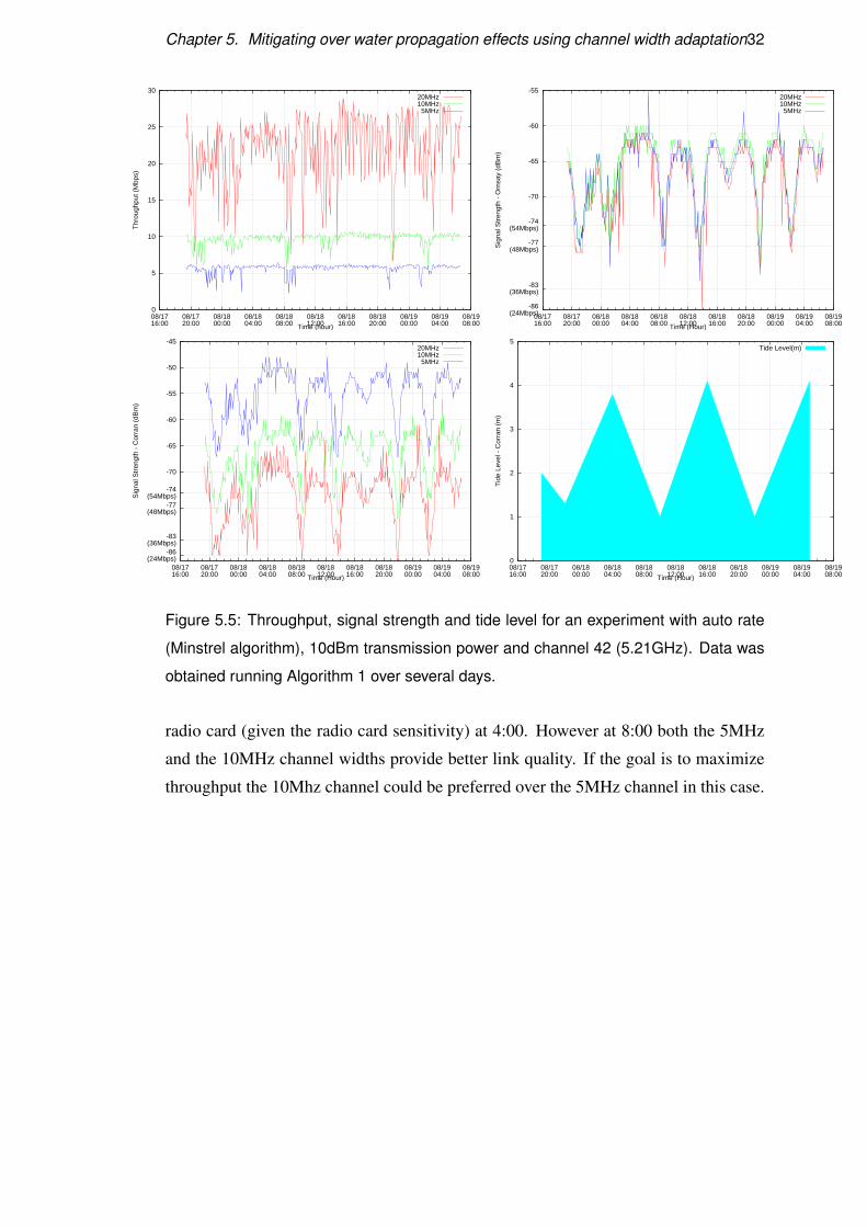
Chapter 5. Mitigating over water propagation effects using channel width adaptation32

0

5

10

15

20

25

30

08/1716:00

08/1720:00

08/1800:00

08/1804:00

08/1808:00

08/1812:00

08/1816:00

08/1820:00

08/1900:00

08/1904:00

08/1908:00

Thr

ough

put (

Mbp

s)

Time (hour)

20MHz10MHz5MHz

-86(24Mbps)

-83(36Mbps)

-77(48Mbps)

-74(54Mbps)

-70

-65

-60

-55

08/1716:00

08/1720:00

08/1800:00

08/1804:00

08/1808:00

08/1812:00

08/1816:00

08/1820:00

08/1900:00

08/1904:00

08/1908:00

Sig

nal S

tren

gth

- O

rnsa

y (d

Bm

)

Time (Hour)

20MHz10MHz5MHz

-86(24Mbps)

-83(36Mbps)

-77(48Mbps)

-74(54Mbps)

-70

-65

-60

-55

-50

-45

08/1716:00

08/1720:00

08/1800:00

08/1804:00

08/1808:00

08/1812:00

08/1816:00

08/1820:00

08/1900:00

08/1904:00

08/1908:00

Sig

nal S

tren

gth

- C

orra

n (d

Bm

)

Time (Hour)

20MHz10MHz5MHz

0

1

2

3

4

5

08/1716:00

08/1720:00

08/1800:00

08/1804:00

08/1808:00

08/1812:00

08/1816:00

08/1820:00

08/1900:00

08/1904:00

08/1908:00

Tid

e Le

vel -

Cor

ran

(m)

Time (Hour)

Tide Level(m)

Figure 5.5: Throughput, signal strength and tide level for an experiment with auto rate

(Minstrel algorithm), 10dBm transmission power and channel 42 (5.21GHz). Data was

obtained running Algorithm 1 over several days.

radio card (given the radio card sensitivity) at 4:00. However at 8:00 both the 5MHz

and the 10MHz channel widths provide better link quality. If the goal is to maximize

throughput the 10Mhz channel could be preferred over the 5MHz channel in this case.

Chapter 5. Mitigating over water propagation effects using channel width adaptation33

0

500

1000

1500

2000

2500

3000

3500

4000

4500

08/1716:00

08/1720:00

08/1800:00

08/1804:00

08/1808:00

08/1812:00

08/1816:00

08/1820:00

08/1900:00

08/1904:00

08/1908:00

UD

P p

acke

ts lo

st

Time (hour)

20MHz10MHz5MHz

Figure 5.6: Packet loss at the Ornsay node using auto rate (Minstrel algorithm), 10dBm

transmission power and channel 42 (5.21GHz).

Chapter 6

Conclusions and future work

The simulation of a long-distance wireless link using the Pathloss software contributed

to explore and understand how different diversity mechanisms (namely center of fre-

quency, polarization and antenna height adaptation) mitigate the negative effects of

tide levels on the signal strength.

Studying the different forms of diversity raised the question whether the adaptation

of the channel width might be a feasible mechanism to mitigate the effects of tide lev-

els on link quality. After a process involving the upgrade and deployment of software

supporting variable channel widths on real hardware, the effect of channel widths on

different network variables was investigated. The obtained experimental indoor repro-

duced previous findings by Chandra[3].

The deployment of the necessary upgrades to support variable channel widths on

the Tegola network, allowed the evaluation of the effect of variable channel widths in

the presence of tidal effects. The outdoor experimental results suggest that adapting

the channel width improves the signal strength at the transmitter.

Additionally, the expertise gained by the author on-site, i.e. 1) by deploying the

boards on the existing Tegola nodes and the 2) setting up the new Li ↔ Corran link

might be useful in the future to setup long-distance links using IEEE 802.11 technolo-

gies in other locations. The lessons learned from this stage of the project can help

future researchers using the Tegola network as a testbed.

Several lines of future research can be derived from this work. While the synchro-

nization algorithm described in 4.2 works at application level and requires an additional

channel for message passing, algorithms which don’t require an additional interface,

but perform negotiation of the channel width and center of frequency at the MAC layer

could be developed. The implementation of such algorithms might require to heavily

34

Chapter 6. Conclusions and future work 35

modify the radio card driver.

Second, the measurements on the Corran ↔ Ornsay long-distance link, show the

behavior of a high quality link with virtually no interference. The role of channel

widths in noisy long-distance links might be worth exploring.

Finally, the simulation results obtained with Pathloss can be used to help extend

network simulation software such as Qualnet1 with a new adaptation protocols that

include support for variable channel widths and that take decisions based on models of

tidal effects.

1http://www.scalable-networks.com/products/developer.php

Appendix A

Basic concepts

The concepts defined in sections A.1 and A.2 are based on the given in the books [16]

and [17].

A.1 Signals

Every electromagnetic signal can be modeled as a function of time or a function of

frequency. As a function of time s(t) a signal is characterized by its amplitude (A),

frequency ( f ) and phase (ϕ). For digital communications the fundamental (periodic)

signal is the sine signal: s(t) = Asin(2π f t +ϕ), with s(t) the peak amplitude (usually

in volts) at time t.

A real-world signal don’t comprise only one frequency but many. In particular, the

periodic square wave signal with amplitude A used for digital communications (a signal

that can be used to carry 1s and 0s) can be approximated with the sum of different sine

signals with different, in theory an infinite number of, frequencies1:

s(t) =4Aπ

∑k∈N(odd)

1k

sin(2πk f t) (A.1)

The spectrum of a signal is the range of frequencies comprised by it. For example,

the signal of amplitude 1 described by

s(t) =4π(sin(2π f t)+

13

sin(2π(3 f )t)+15

sin(2π(5 f )t) (A.2)

has a spectrum in the range [ f . . .5 f ]. The signal width (Sw) is the width of the

signal’s spectrum. A.2 has a width of 5 f −1 f = 4 f .1By definition s(t) is an infinite sum however the value of the terms in the sum tend to 0 as k tends

to ∞.

36

Appendix A. Basic concepts 37

Signal width and data rate are related. Suppose the square wave signal A.2 with

f = 1MHz = 106cycles/second. The width of the signal is 4 f = 4MHz and its period is

T = 1/ f = 10−6seconds. Assuming that 2 bits (a 1 followed by a 0) can be carried by

each cycle, a bit can be transmitted every 0.5µs, that is at a rate of 2 ·106bits/second =

2Mbps2.

Given a signal with a spectrum in the range [α . . .β] the center frequency of the

signal is given by Sc = (β−α)/2. It’s said such a signal is centered about frequency

Sc. In the previous example s(t) is centered about Sc = 2MHz with width Sw = 4MHz.

A.2 Channel characterization

A communication channel (C) is composed by a physical medium and a device capable

of transmitting information in signal form. When applying an arbitrary periodic signal

s(t) to C, say the square wave signal in equation A.3, the channel attenuates/delays the

input signal. The output signal of the channel is an attenuated/delayed signal s′(t)

s′(t) = ∑k∈N(odd)

akA(k f )sin(2πk f t +ϕ(k f )) (A.3)

with A(k f ) the ratio of the amplitude (power) of the input and output signals at

frequency k f (attenuation factor) and ϕ(k f ) the change in phase between the output

and input signals at frequency k f (delay factor). The combination of A and ϕ can be

understood as a filter that modifies the frequency components of a signal. The width of

the range of frequencies (spectrum) [β . . .γ] that a channel, understood as a filter, allows

to pass to the medium is called the channel width (Fw). The range of frequencies passed

by a channel can also be thought as centered about a frequency Fc = (γ−β)/2 with

channel width Fw. A channel can be characterized by the pair 〈Fc,Fw〉.

2It’s possible to obtain a different data rate given the same signal width by using a different squarewave signal. I.e. the same width might support different data rates.

Appendix B

Link planning with SPLAT

This appendix briefly describes the way SPLAT was used to verify the line-of-sight

nature of the Li ↔ Corran link. Unlike other link planning tools like RadioMobile,

SPLAT and command-line based and free software (GNU GPL license).

The following input data is given to SPLAT to obtain the line-of-sight and Longley-

Rice analysis.

• Site location files: These files contain the geographical coordinates of the link’s

nodes. For the test link the contents of the files where:

$ cat li.qth

Li

57.107313

5.578911

9 meters

$ cat corran.qth

Corran

57.12455

5.551056

44 meters

• Antenna radiation pattern files: The azimuth and elevation files are used to de-

fine the direction of the radiation emitted by the antenna. The files are called

corran.az and corran.el, analogous for the Li node. The radiation patterns

are shown in Figure B.1.

• Terrain files. The terrain files were obtained from http://dds.cr.usgs.gov/

srtm/version2/SRTM3/Eurasia/.

• Longley-Rice parameters. The following file was used:

80.000 ; Earth Dielectric Constant (Relative permittivity)

5.000 ; Earth Conductivity (Siemens per meter)

38

Appendix B. Link planning with SPLAT 39

20

15

10

5

0

5

10

15

20

15 10 5 0 5 10 15 20

dBm

dBm

Azimuth antenna radiation pattern used for path analysis

Antenna gain

0.04

0.02

0

0.02

0.04

0.06

0.08

0.1

0.12

0.14

0.16

0.18

0 0.1 0.2 0.3 0.4 0.5 0.6 0.7 0.8 0.9 1

dBm

dBm

Elevation antenna radiation pattern used for path analysis

Antenna gain

Figure B.1: Directional antenna’s azimuth (left) and elevation (right) radiation pat-

terns used for SPLAT.

301.000 ; Atmospheric Bending Constant (N-Units)

5400.000 ; Frequency in MHz (20 MHz to 20 GHz)

5 ; Radio Climate

1 ; Polarization (0 = Horizontal, 1 = Vertical)

0.50 ; Fraction of situations

0.90 ; Fraction of time

With

splat -t li.qth -r corran.qth -kml -metric

The Longley-Rice analysis results are written to the Li-to-Corran.txt file. The

Li-to-Corran.kml is also generated and can be imported into GoogleEarth to visu-

alize the line-of-sight between the two nodes. This visualization is shown in Figure

B.2.

Appendix B. Link planning with SPLAT 40

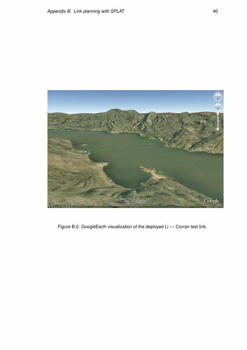
Figure B.2: GoogleEarth visualization of the deployed Li↔ Corran test link.

Appendix C

Greedy edge coloring implementation

During the first days of the project the graph theoretical approach to center of frequency

allocation was explored. As mentioned in Section 1, Dutta[2] proposes an algorithm

for channel allocation using this approach.

The main objective of this contribution was to gain insight on the implementation

of simple graph theoretical algorithms relevant for static channel allocation, using the

C++ Boost Graph Library (BGL)1.

The problem of edge coloring is to assign a color (or weight) to all edges in a graph,

in such a way that no two adjacent vertices get the same color. An optimal solution

finds a minimal number of weights to color the graph. Let G = (E,V ) an undirected

graph. Two edges e1,e2∈ E are adjacent if they share a vertex. This problem is in NP,

i.e. there is no generic deterministic algorithm that solves it in polynomial time.

However, a greedy algorithm for edge coloring, though not optimal, is very near to

the optimal solution and surprisingly very fast. Algorithm 2 was implemented using

the BGL. The implementation is able to color the edges of graph with 50 edges and

nearly 800 vertices in less of a half of a second2.

1http://www.boost.org/doc/libs/1_39_0/libs/graph/doc/index.html2On an Intel(R) Core(TM)2 Duo CPU T5450 @ 1.66GHz CPU.

41

Appendix C. Greedy edge coloring implementation 42

Algorithm 2 Greedy edge coloring1: procedure GREEDYEDGECOLORING(G = (E,V )) . G undirected graph

2: color map← /0

3: while |color map|< |E| do4: e← random edge(G) . Pick an edge randomly

5: if e /∈ color map then6: c← ad jacent colors(e,G) . Get the colors of the adjacent edges

7: color map[e]← max(c)+1 . e has lowest possible color

8: end if9: end while

10: return color map

11: end procedure

The greedy algorithm isn’t optimal. Moreover, the use case of the algorithm is to

assign centers of frequency, the maximum number of colors obtained by the algorithm

might exceed the number of available channels. A naive approach which just uses

the modulo operation to constraint the number of different colors to the number of

available channels is shown in Algorithm 3. Obviously Algorithm 3 won’t preserve

the invariant of the edge coloring algorithm, i.e. adjacent edges might receive the same

color.

Algorithm 3 Channel mapping1: procedure CHANNELMAPPING(G = (E,V ),color map,num channels)

2: num colors← max(color map)

3: if num colors <= num channels then4: nop . There are enough channels to color the edges

5: else6: for entry ∈ color map do7: entry.color = entry.color%num channels . Limit to channels

8: end for9: end if

10: return color map

11: end procedure

Here an example of usage of the implementation of algorithms,

$ graph_driver --input-file=graph.txt --nc 4

Appendix C. Greedy edge coloring implementation 43

Number of channels is: 4

Input file is: graph.txt

Result:

(0,3)->2

(0,1)->3

(3,2)->1

(2,0)->6

(3,4)->6

(1,3)->7

(2,4)->5

(4,1)->4

(4,0)->1

Max color:7 (Number of channels:4)

Adjusting mapping. There are no enough channels to color the edges!

(0,3)->3

(0,1)->4

(3,2)->2

(2,0)->3

(3,4)->3

(1,3)->4

(2,4)->2

(4,1)->1

(4,0)->2

The C++ implementation of the algorithm is available with git at the URL git@

github.com:jhairtt/graph_driver.

Bibliography

[1] Giacomo Bernardi, Peter Buneman, and Mahesh K. Marina. Tegola tiered mesh

network testbed in rural scotland. In Wireless Networks and Systems for Devel-

oping Regions, pages 9–16, 2008.

[2] P. Dutta, S. Jaiswal, D. Panigrahi, and R. Rastogi. A new channel assignment

mechanism for rural wireless mesh networks. INFOCOM 2008. The 27th Con-

ference on Computer Communications. IEEE, pages 2261–2269, April 2008.

[3] Ranveer Chandra, Ratul Mahajan, Thomas Moscibroda, Ramya Raghavendra,

and Paramvir Bahl. A case for adapting channel width in wireless networks. In

SIGCOMM, pages 135–146, 2008.

[4] Ramakrishna Gummadi, Rabin Patra, Hari Balakrishnan, and Eric Brewer. Inter-

ference Avoidance and Control. In 7th ACM Workshop on Hot Topics in Networks

(Hotnets-VII), Calgary, Canada, October 2008.

[5] Office of Communications Offcom. UK Interface Requirement 2007. Fixed

broadband services operating in the 5725-5860 MHz band. http://www.ofcom.

org.uk/radiocomms/ifi/tech/interface_req/uk_interface_2007.pdf,

May 2007.

[6] Solwise Ltd. Pointers on using the 5GHz WiFi bands. http://www.

solwiseforum.co.uk/downloads/files/intheuk5ghz.pdf, May 2007.

[7] Kameswari Chebrolu, Bhaskaran Raman, and Sayandeep Sen. Long-distance

802.11b links: performance measurements and experience. In MobiCom ’06:

Proceedings of the 12th annual international conference on Mobile computing

and networking, pages 74–85, New York, NY, USA, 2006. ACM.

[8] D. Gokhale, S. Sen, K. Chebrolu, and B. Raman. On the feasibility of the link

44

Bibliography 45

abstraction in (rural) mesh networks. INFOCOM 2008. The 27th Conference on

Computer Communications. IEEE, pages 61–65, April 2008.

[9] A. Sheth, S. Nedevschi, R. Patra, S. Surana, E. Brewer, and L. Subramanian.

Packet loss characterization in wifi-based long distance networks. INFOCOM

2007. 26th IEEE International Conference on Computer Communications. IEEE,

pages 312–320, May 2007.

[10] T. Ireland, A. Nyzio, M. Zink, and J. Kurose. The impact of directional antenna

orientation, spacing, and channel separation on long-distance multi-hop 802.11g

networks: A measurement study. In Modeling and Optimization in Mobile, Ad

Hoc and Wireless Networks and Workshops, 2007. WiOpt 2007. 5th International

Symposium on, pages 1–6, April 2007.

[11] Bhaskaran Raman and Kameswari Chebrolu. Design and evaluation of a new

mac protocol for long-distance 802.11 mesh networks. In MobiCom ’05: Pro-

ceedings of the 11th annual international conference on Mobile computing and

networking, pages 156–169, New York, NY, USA, 2005. ACM.

[12] Sergiu Nedevschi, Rabin K. Patra, Sonesh Surana, Sylvia Ratnasamy, Lakshmi-

narayanan Subramanian, and Eric Brewer. An adaptive, high performance mac

for long-distance multihop wireless networks. In MobiCom ’08: Proceedings

of the 14th ACM international conference on Mobile computing and networking,

pages 259–270, New York, NY, USA, 2008. ACM.

[13] I. Wormsbecker and C. Williamson. On channel selection strategies for multi-

channel mac protocols in wireless ad hoc networks. In Wireless and Mobile

Computing, Networking and Communications, 2006. (WiMob’2006). IEEE In-

ternational Conference on, pages 212–220, June 2006.

[14] Christopher Haslett. Essentials of Radio Wave Propagation. Cambridge Univer-

sity Press, 1st edition, 2007.

[15] Jangeun Jun, Pushkin Peddabachagari, and Mihail Sichitiu. Theoretical Maxi-

mum Throughput of IEEE 802.11 and its Applications. In NCA ’03: Proceed-

ings of the Second IEEE International Symposium on Network Computing and

Applications, page 249, Washington, DC, USA, 2003. IEEE Computer Society.

Bibliography 46

[16] A. Leon-Garcia and I. Widjaja. Communication Networks: Fundamental Con-

cepts and Key Architectures. Mc Graw Hill, 2003.

[17] William Stallings. Data and computer communications (5th ed.). Prentice-Hall,

Inc., Upper Saddle River, NJ, USA, 1997.