1

Immobile Australia: Surnames show Strong Status Persistence, 1870-20171 Gregory Clark, UC Davis (glark@ucdavis.edu) Andrew Leigh, Parliament of Australia, (Andrew.Leigh.MP@aph.gov.au) Mike Pottenger, Melbourne University (mpotteng@unimelb.edu.au)

The paper estimates long run social mobility in Australia 1870-2017 tracking the status of rare surnames. The status information includes occupations from electoral rolls 1903-1980, and records of degrees awarded by Melbourne and Sydney universities 1852-2017. Status persistence was strong throughout, with an intergenerational correlation of 0.7-0.8, and no change over time. Notwithstanding egalitarian norms, high immigration and a well-targeted social safety net, Australian long-run social mobility rates are low. Despite evidence on conventional measures that Australia has higher rates of social mobility than the UK or USA (Mendolia and Siminski, 2016), status persistence for surnames is as high as that in England or the USA. Mobility rates are also just as low if we look just at mobility within descendants of UK immigrants, so ethnic effects explain none of the immobility.

The Son Also Rises (Clark et al., 2014) showed that grouping people by surnames or surname types consistently reveals intergenerational correlations of status measures such as wealth, education, and occupational status in the range 0.7-0.8 for a wide variety of countries. England in particular shows this pattern of slow mobility 1800-2015 (Clark and Cummins, 2015). This correlation is much greater than the correlation observed on such measures between parent and child. The surname correlation in status also varied little between countries and time periods. To explain this difference in intergenerational correlations at the surname versus the individual level Clark et al., 2014, posited that social mobility has the following structure. If y is the measured status of individuals (measured with mean 0 and a constant variance), then

1 We thank Sarah Banks and Margaret Sheil at Melbourne University for access to graduation records. We thank Lujia Wang for research assistance.

2

𝑦𝑦𝑡𝑡 = 𝑥𝑥𝑡𝑡 + 𝑢𝑢𝑡𝑡 (1)

𝑥𝑥𝑡𝑡 = 𝑏𝑏𝑥𝑥𝑡𝑡−1 + 𝑒𝑒𝑡𝑡 (2) where xt is the family’s underlying social competence, and ut is the random component, and b is the intergenerational correlation of underlying status. The above implies that the conventional studies of social mobility, based on estimating the intergenerational correlation β in the relationship

𝑦𝑦𝑡𝑡+1 = 𝛽𝛽𝑦𝑦𝑡𝑡 + 𝑣𝑣𝑡𝑡 (3) for various partial measures of status—earnings, wealth, education, occupation and so on —underestimates the true intergenerational correlation b that links underlying social status across generations. In particular, the expected value of conventional

estimates β is not the underlying b but instead θb, where θ = 𝜎𝜎𝑢𝑢2

𝜎𝜎𝑥𝑥2+ 𝜎𝜎𝑢𝑢2 is less than

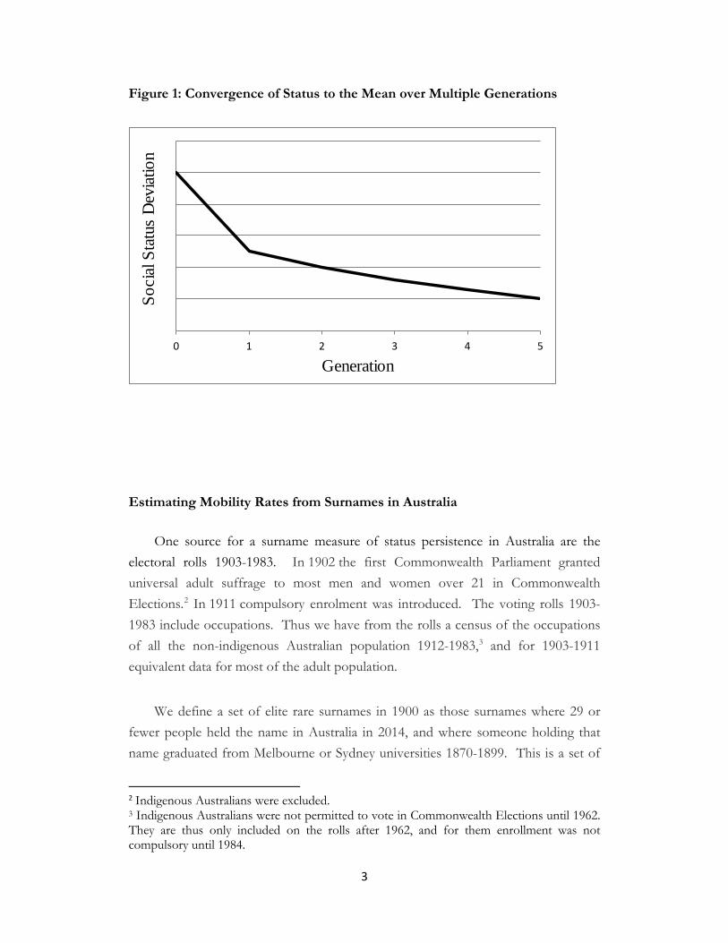
one. Further, the greater the random components of any measured aspect of status, the smaller will θ be. With the specification of equations (1) and (2) the observed pattern on any status measure, as a deviation from the mean, will look as in figure 1 for an individual observed with higher than average status in the initial period. The rate of convergence to the mean will decline greatly after the first generation, and will be at a constant low rate thereafter. The higher long run intergenerational correlation in figure 1 will be the one that applies for social groups. It will also be closer than conventional measures to the intergenerational correlation when we consider a more comprehensive measure of family status than individual aspects such as income, education or occupational status. In this paper we derive equivalent surname status correlations for Australia 1870-2017. These show that despite the fact that Australia was an immigrant society incorporating migrants from a wide variety of backgrounds, and without some of the entrenched social institutions and rigidities of England, underlying social mobility rates all the way from 1870 to 2017 were just as slow as in England. Also there is no sign of any increase in mobility rates in the most recent years.

3

Figure 1: Convergence of Status to the Mean over Multiple Generations

Estimating Mobility Rates from Surnames in Australia

One source for a surname measure of status persistence in Australia are the electoral rolls 1903-1983. In 1902 the first Commonwealth Parliament granted universal adult suffrage to most men and women over 21 in Commonwealth Elections.2 In 1911 compulsory enrolment was introduced. The voting rolls 1903-1983 include occupations. Thus we have from the rolls a census of the occupations of all the non-indigenous Australian population 1912-1983,3 and for 1903-1911 equivalent data for most of the adult population.

We define a set of elite rare surnames in 1900 as those surnames where 29 or fewer people held the name in Australia in 2014, and where someone holding that name graduated from Melbourne or Sydney universities 1870-1899. This is a set of

2 Indigenous Australians were excluded. 3 Indigenous Australians were not permitted to vote in Commonwealth Elections until 1962. They are thus only included on the rolls after 1962, and for them enrollment was not compulsory until 1984.

0 1 2 3 4 5

Soci

al St

atus

Dev

iatio

n

Generation

4

159 surnames. Then for the benchmark years 1903-1907, 1926-1930, 1954, 1980 we calculate the average status of these surnames, for men, in each period t as

𝑍𝑍𝑡𝑡 = ∑𝑦𝑦𝑖𝑖𝑖𝑖𝑖𝑖− 𝑦𝑦�

𝜎𝜎𝑥𝑥 (4)

where y is an index of occupational status for each occupation, derived below, j indexes the rare elite surnames, i indexes the individual men with that surname, 𝑦𝑦� is the mean of occupational status in the population as a whole, 𝜎𝜎𝑦𝑦 is the standard deviation of occupational status in the male population. The intergenerational correlation of status across each period was calculated as

𝜌𝜌 = �𝑍𝑍𝑖𝑖+𝑛𝑛𝑍𝑍𝑖𝑖�30𝑛𝑛 (5)

This assumes that a generation is 30 years. Thus the intergenerational correlation between 1954 and 1980 is

𝜌𝜌 = �𝑍𝑍1980𝑍𝑍1954

�1.15

(6)

Can we be sure that this correlation 𝜌𝜌 will correspond to the underlying correlation of status at the family level as posited in equations (1) and (2)? In many cases, for example, the same person will appear in the 1903 electoral roll and in the 1928 electoral roll. Will that not drive up the measured correlation? However, intuitively, what we are doing is comparing people observed in 1904, born 1839-1883, with people born on average 25 years later, 1864-1908. Thus while there will be some people who are observed in both samples, there will also be an equivalent sized group where the relationship is across three generations, grandfather to grandson. As long as there is a constant underlying intergenerational correlation, on average we will be observing a correlation close to that for one generation. We can demonstrate the correctness of this intuition with some data from England where for a group of surnames that were high wealth for deaths 1858-1887 we have measures of occupational status for men born 1838-1925, as well as all the individual family links. We can thus calculate the underlying intergenerational

5

correlation of status for these men 1904-1929 using the method proposed here for the Australian data, and compare that to the intergenerational correlation estimated from actual father-son links in the relevant period. We calculate average occupational status for the group for all men alive in 1904 aged 21-65, and for all men alive in 1929 aged 21-65. We calculate using equation (4) this status as deviations from the mean in standard deviation units where for a group of average status surnames we can calculate mean occupational status, and also the standard deviation of occupational status. The high status men move from being 1.80 standard deviations above average in status 1904, to being 1.44 standard deviations above average status in 1929. Normalized to a generation length of 30 years, this implies from equation (5), an intergenerational correlation of 0.77. If instead we calculate the intergenerational correlation of status by taking the deviation in average status of fathers alive in 1904 and aged 21-65 and comparing that with their sons’ average deviation then those numbers are 1.42 standard deviations and 1.15, and the implied intergenerational correlation is 0.78. Thus the two methods of estimation produce very similar results here. To derive mean population occupation status for the relevant social group in Australia we used a sample of occupations for the common surname Smith (and variants such as Smyth) for each benchmark period. Smith was chosen since the majority of the rare surnames were British and Irish in origin, so this would be the relevant comparison group.

For 1980 to assign social status to each occupation we use the index of occupational status for Australia derived by Broom, Jones, Duncan-Jones, and McDonnell, 1977 (ANU2). Scores ranged from 331 (laborers) to 896 (industrial efficiency engineers). We also checked the robustness of the results by also applying the ANU3 scale derived by Jones, 1989. Scores on ANU3 were scaled to range from 0 (low status) to 100 (high status). Status scores for ANU3 were assigned based on occupational prestige ratings and worker characteristics from the 1986 census. For 1954 we also applied the ANU2 scale.

In addition for 1903, 1928 and 1954 we applied a scale derived from English occupation data 1841-1929, where that scale was based for each occupation on reported wealth at death, higher educational attainment, and probability of being at work aged 11-20.

6

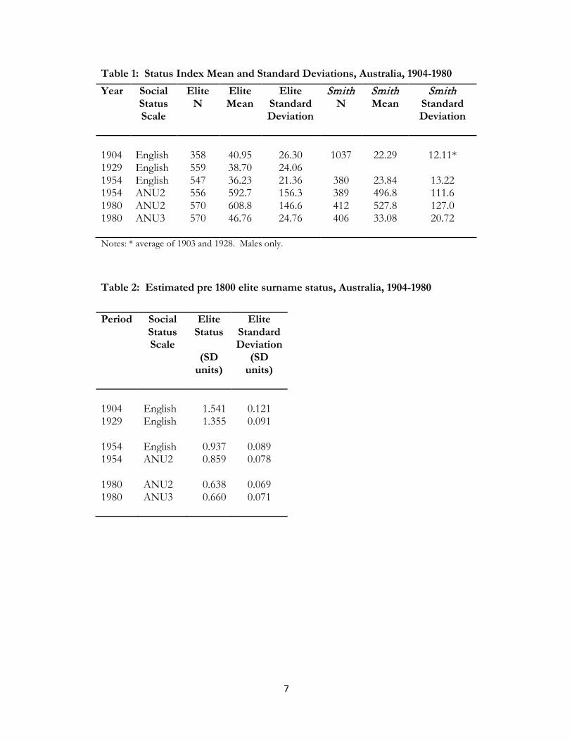
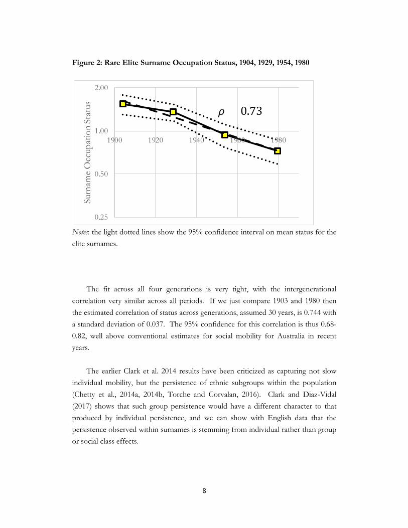
Table 2 shows the estimated average status of the sample of the elite Australian surname in each period, as well as the estimated average status of the equivalent population as a whole derived from the Smith sample. Table 2 shows the implied deviation of the elite surnames from average status in standard deviation units in each years and each status measure. Also shown is the standard deviation of these mean status estimates for the elite surnames. As can be seen the elite surnames deviate very significantly, in quantitative and statistical terms, from mean surname status even in 1980. These surnames, remember, were identified as high status based on someone with the surname graduating from Melbourne or Sydney Universities before 1900. This shows the slowness of social mobility in twentieth century Australia. Figure 2 shows the estimated status of the elite surnames at each benchmark, measured in standard deviation units above mean social status, as well as the 5% confidence interval around these estimates. Also shown is the best fitting estimate with a constant rate of intergenerational mobility from 1904 to 1980. The best fitting correlation of status across generations for the whole period is 0.73.

7

Table 1: Status Index Mean and Standard Deviations, Australia, 1904-1980 Year Social

Status Scale

Elite N

Elite Mean

Elite Standard Deviation

Smith N

Smith Mean

Smith Standard Deviation

1904 English 358 40.95 26.30 1037 22.29 12.11* 1929 English 559 38.70 24.06 1954 English 547 36.23 21.36 380 23.84 13.22 1954 ANU2 556 592.7 156.3 389 496.8 111.6 1980 ANU2 570 608.8 146.6 412 527.8 127.0 1980 ANU3 570 46.76 24.76 406 33.08 20.72 Notes: * average of 1903 and 1928. Males only.

Table 2: Estimated pre 1800 elite surname status, Australia, 1904-1980

Period Social Status Scale

Elite Status

(SD

units)

Elite Standard Deviation

(SD units)

1904 English 1.541 0.121 1929

English 1.355 0.091

1954 English 0.937 0.089 1954

ANU2 0.859 0.078

1980 ANU2 0.638 0.069 1980 ANU3 0.660 0.071

8

Figure 2: Rare Elite Surname Occupation Status, 1904, 1929, 1954, 1980

Notes: the light dotted lines show the 95% confidence interval on mean status for the elite surnames.

The fit across all four generations is very tight, with the intergenerational correlation very similar across all periods. If we just compare 1903 and 1980 then the estimated correlation of status across generations, assumed 30 years, is 0.744 with a standard deviation of 0.037. The 95% confidence for this correlation is thus 0.68-0.82, well above conventional estimates for social mobility for Australia in recent years. The earlier Clark et al. 2014 results have been criticized as capturing not slow individual mobility, but the persistence of ethnic subgroups within the population (Chetty et al., 2014a, 2014b, Torche and Corvalan, 2016). Clark and Diaz-Vidal (2017) shows that such group persistence would have a different character to that produced by individual persistence, and we can show with English data that the persistence observed within surnames is stemming from individual rather than group or social class effects.

0.25

0.50

1.00

2.00

1900 1920 1940 1960 1980

Surn

ame

Occ

upat

ion

Stat

us 𝜌𝜌 = 0.73

9

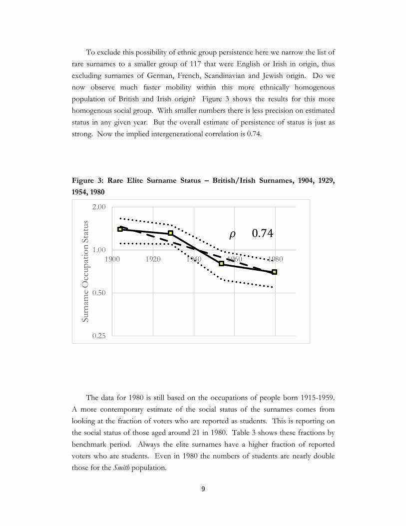
To exclude this possibility of ethnic group persistence here we narrow the list of rare surnames to a smaller group of 117 that were English or Irish in origin, thus excluding surnames of German, French, Scandinavian and Jewish origin. Do we now observe much faster mobility within this more ethnically homogenous population of British and Irish origin? Figure 3 shows the results for this more homogenous social group. With smaller numbers there is less precision on estimated status in any given year. But the overall estimate of persistence of status is just as strong. Now the implied intergenerational correlation is 0.74. Figure 3: Rare Elite Surname Status – British/Irish Surnames, 1904, 1929, 1954, 1980

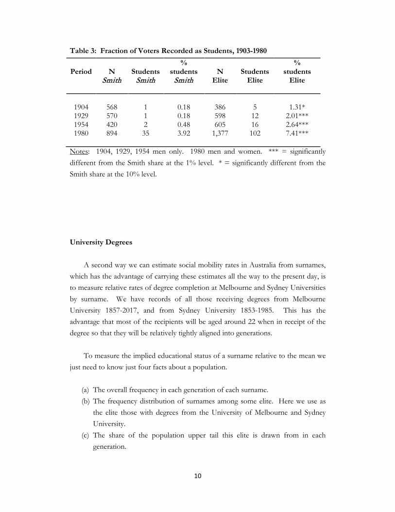
The data for 1980 is still based on the occupations of people born 1915-1959. A more contemporary estimate of the social status of the surnames comes from looking at the fraction of voters who are reported as students. This is reporting on the social status of those aged around 21 in 1980. Table 3 shows these fractions by benchmark period. Always the elite surnames have a higher fraction of reported voters who are students. Even in 1980 the numbers of students are nearly double those for the Smith population.

0.25

0.50

1.00

2.00

1900 1920 1940 1960 1980

Surn

ame

Occ

upat

ion

Stat

us

𝜌𝜌 = 0.74

10

Table 3: Fraction of Voters Recorded as Students, 1903-1980

Period

N

Smith

Students

Smith

% students

Smith

N

Elite

Students

Elite

% students

Elite

1904 568 1 0.18 386 5 1.31* 1929 570 1 0.18 598 12 2.01*** 1954 420 2 0.48 605 16 2.64*** 1980 894 35 3.92 1,377 102 7.41***

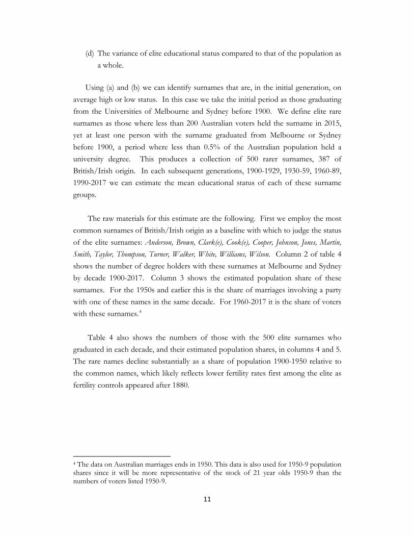
Notes: 1904, 1929, 1954 men only. 1980 men and women. *** = significantly different from the Smith share at the 1% level. * = significantly different from the Smith share at the 10% level. University Degrees A second way we can estimate social mobility rates in Australia from surnames, which has the advantage of carrying these estimates all the way to the present day, is to measure relative rates of degree completion at Melbourne and Sydney Universities by surname. We have records of all those receiving degrees from Melbourne University 1857-2017, and from Sydney University 1853-1985. This has the advantage that most of the recipients will be aged around 22 when in receipt of the degree so that they will be relatively tightly aligned into generations. To measure the implied educational status of a surname relative to the mean we just need to know just four facts about a population.

(a) The overall frequency in each generation of each surname. (b) The frequency distribution of surnames among some elite. Here we use as

the elite those with degrees from the University of Melbourne and Sydney University.

(c) The share of the population upper tail this elite is drawn from in each generation.

11

(d) The variance of elite educational status compared to that of the population as a whole.

Using (a) and (b) we can identify surnames that are, in the initial generation, on

average high or low status. In this case we take the initial period as those graduating from the Universities of Melbourne and Sydney before 1900. We define elite rare surnames as those where less than 200 Australian voters held the surname in 2015, yet at least one person with the surname graduated from Melbourne or Sydney before 1900, a period where less than 0.5% of the Australian population held a university degree. This produces a collection of 500 rarer surnames, 387 of British/Irish origin. In each subsequent generations, 1900-1929, 1930-59, 1960-89, 1990-2017 we can estimate the mean educational status of each of these surname groups.

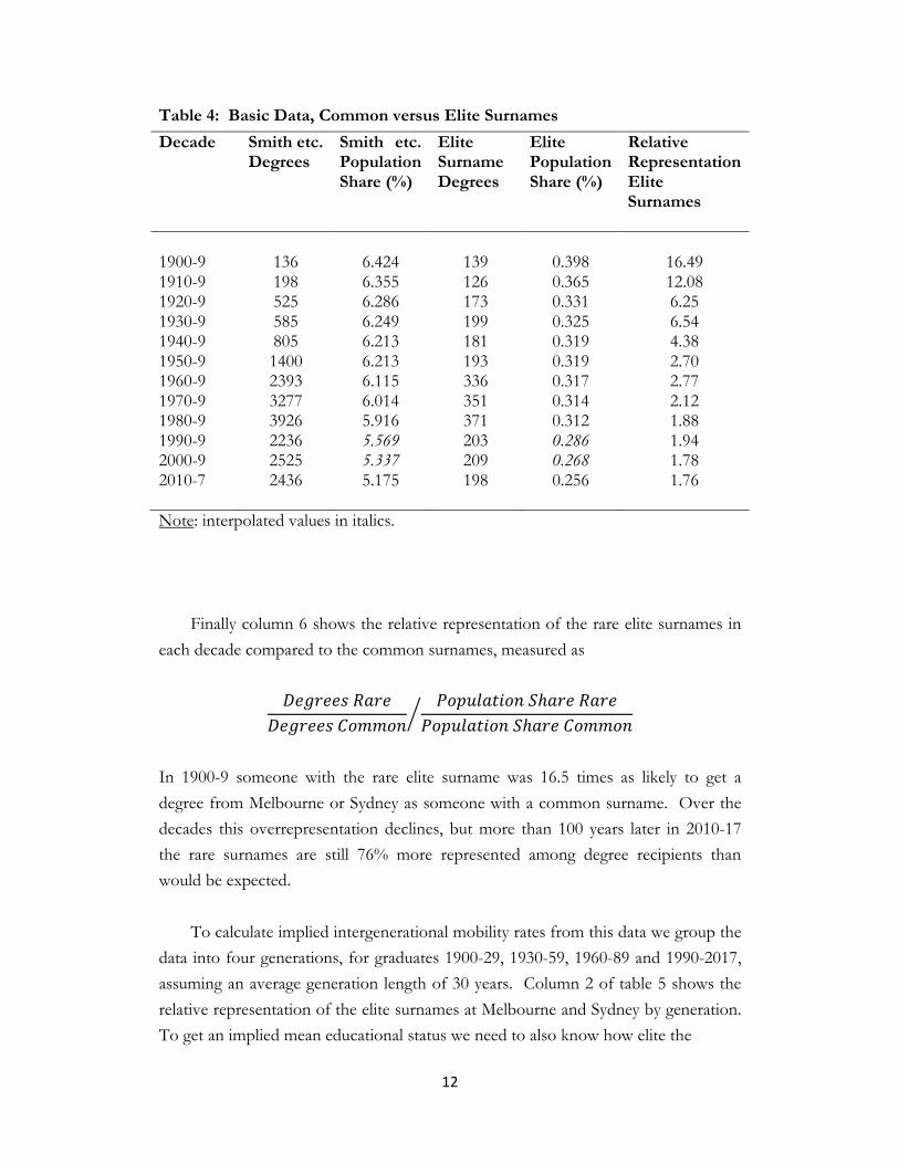
The raw materials for this estimate are the following. First we employ the most common surnames of British/Irish origin as a baseline with which to judge the status of the elite surnames: Anderson, Brown, Clark(e), Cook(e), Cooper, Johnson, Jones, Martin, Smith, Taylor, Thompson, Turner, Walker, White, Williams, Wilson. Column 2 of table 4 shows the number of degree holders with these surnames at Melbourne and Sydney by decade 1900-2017. Column 3 shows the estimated population share of these surnames. For the 1950s and earlier this is the share of marriages involving a party with one of these names in the same decade. For 1960-2017 it is the share of voters with these surnames.4

Table 4 also shows the numbers of those with the 500 elite surnames who

graduated in each decade, and their estimated population shares, in columns 4 and 5. The rare names decline substantially as a share of population 1900-1950 relative to the common names, which likely reflects lower fertility rates first among the elite as fertility controls appeared after 1880.

4 The data on Australian marriages ends in 1950. This data is also used for 1950-9 population shares since it will be more representative of the stock of 21 year olds 1950-9 than the numbers of voters listed 1950-9.

12

Table 4: Basic Data, Common versus Elite Surnames Decade Smith etc.

Degrees

Smith etc. Population Share (%)

Elite Surname Degrees

Elite Population Share (%)

Relative Representation Elite Surnames

1900-9 136 6.424 139 0.398 16.49 1910-9 198 6.355 126 0.365 12.08 1920-9 525 6.286 173 0.331 6.25 1930-9 585 6.249 199 0.325 6.54 1940-9 805 6.213 181 0.319 4.38 1950-9 1400 6.213 193 0.319 2.70 1960-9 2393 6.115 336 0.317 2.77 1970-9 3277 6.014 351 0.314 2.12 1980-9 3926 5.916 371 0.312 1.88 1990-9 2236 5.569 203 0.286 1.94 2000-9 2525 5.337 209 0.268 1.78 2010-7 2436 5.175 198 0.256 1.76 Note: interpolated values in italics.

Finally column 6 shows the relative representation of the rare elite surnames in each decade compared to the common surnames, measured as

𝐷𝐷𝑒𝑒𝐷𝐷𝐷𝐷𝑒𝑒𝑒𝑒𝐷𝐷 𝑅𝑅𝑅𝑅𝐷𝐷𝑒𝑒

𝐷𝐷𝑒𝑒𝐷𝐷𝐷𝐷𝑒𝑒𝑒𝑒𝐷𝐷 𝐶𝐶𝐶𝐶𝐶𝐶𝐶𝐶𝐶𝐶𝐶𝐶𝑃𝑃𝐶𝐶𝑃𝑃𝑢𝑢𝑃𝑃𝑅𝑅𝑃𝑃𝑃𝑃𝐶𝐶𝐶𝐶 𝑆𝑆ℎ𝑅𝑅𝐷𝐷𝑒𝑒 𝑅𝑅𝑅𝑅𝐷𝐷𝑒𝑒

𝑃𝑃𝐶𝐶𝑃𝑃𝑢𝑢𝑃𝑃𝑅𝑅𝑃𝑃𝑃𝑃𝐶𝐶𝐶𝐶 𝑆𝑆ℎ𝑅𝑅𝐷𝐷𝑒𝑒 𝐶𝐶𝐶𝐶𝐶𝐶𝐶𝐶𝐶𝐶𝐶𝐶�

In 1900-9 someone with the rare elite surname was 16.5 times as likely to get a degree from Melbourne or Sydney as someone with a common surname. Over the decades this overrepresentation declines, but more than 100 years later in 2010-17 the rare surnames are still 76% more represented among degree recipients than would be expected. To calculate implied intergenerational mobility rates from this data we group the data into four generations, for graduates 1900-29, 1930-59, 1960-89 and 1990-2017, assuming an average generation length of 30 years. Column 2 of table 5 shows the relative representation of the elite surnames at Melbourne and Sydney by generation. To get an implied mean educational status we need to also know how elite the

13

Table 5: Elite Rare Surname Status, 1900-2017

Degree

Relative Representation of Surnames at

Melbourne and Sydney

Melbourne &Sydney

elite share

Implied mean status of rare

surnames (S.D. units)

Implied

intergenerational correlation of

status

1900-29 12.58 0.010 1.18 - 1930-59 4.56 0.029 0.78 0.69 1960-89 2.26 0.087 0.51 0.60 1990-2017 1.83 0.140 0.43 0.79 student population at these universities is, (c) above. The estimated cutoff in the educational distribution for attending Melbourne and Sydney by generation is shown in column 3 of table 5. That cutoff is estimated for each decade from the share of males (before 1970) and students as a whole (1970 and later) who graduated from one of the Group of Eight universities in Australia. We can roughly check this calculation by looking at the ATAR scores, Australia’s standardized university admissions test. Appropriately for our purposes, the reference point for the ATAR scale is the year 7 cohort, so it is designed to take account of early school leavers. In effect, the ATAR score represents an individual’s percentile rank in their age cohort. For example, a score of 70 indicates that the person outperformed 70 percent of his or her age cohort, assuming that every person of the same age had taken the tests (Universities Admissions Centre, 2015).

14

In the most recent year, median ATAR scores the main undergraduate degrees at Sydney ranged from 86 to 96, while the median ATAR for admission to Melbourne University’s main undergraduate programs ranged from 93 to 97.5 This suggests that these universities today roughly admit the top 15% of the High School Cohort. What is the intergenerational correlation of educational status implied by these relative representation numbers and the measured eliteness of the universities? To measure this we make the following three assumptions .

(i) Educational status is normally distributed. (ii) The elite surname group from 1853-1899 has the same variance of

educational status 1900-2014 within its members as for the population as a whole. We can see above in table 1 that the elite surnames actually showed a higher variance in status than average surnames. So below we will also make the estimate allowing the elite surname educational variance to be higher than for the population as a whole.

(iii) Subsequent holders of these surnames all descended from the holders of 1900-29.

We consider below how the estimated rates of social mobility will be biased if these three simplifying assumptions do not hold.

With these assumptions we can estimate from the data in columns 2 and 3 of table 5 the implied mean educational status of the holders of the rare surnames 1900-2017, measured in standard deviation units from the population mean. The last column of table 5 shows the implied intergenerational correlation of status across each generation. This averages 0.69. 5 These universities have only recently begun publishing median ATAR scores, after media reports showed that the published cut-off scores could be highly misleading. For Melbourne University, the published medians are for 2016, and are 93 for a Bachelor of Arts, 97 for a Bachelor of Commerce, and 93 for a Bachelor of Science. For Sydney University, the available data are for 2017, and the corresponding median ATARs are 87 for a Bachelor of Arts, 96 for a Bachelor of Commerce, and 86 for a Bachelor of Science. One of us also has access to a microdata file of the entrance scores for all undergraduate students admitted into Australian universities between 1999 and 2005. In these years, Sydney University’s mean entrance score ranged from 86 to 89, while Melbourne University’s mean entrance score ranged from 92 to 93.

15

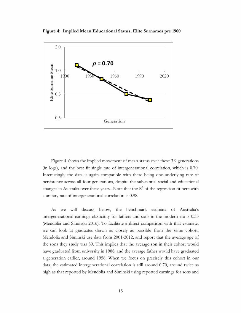
Figure 4: Implied Mean Educational Status, Elite Surnames pre 1900

Figure 4 shows the implied movement of mean status over these 3.9 generations

(in logs), and the best fit single rate of intergenerational correlation, which is 0.70. Interestingly the data is again compatible with there being one underlying rate of persistence across all four generations, despite the substantial social and educational changes in Australia over these years. Note that the R2 of the regression fit here with a unitary rate of intergenerational correlation is 0.98.

As we will discuss below, the benchmark estimate of Australia’s

intergenerational earnings elasticitity for fathers and sons in the modern era is 0.35 (Mendolia and Siminski 2016). To facilitate a direct comparison with that estimate, we can look at graduates drawn as closely as possible from the same cohort. Mendolia and Siminski use data from 2001-2012, and report that the average age of the sons they study was 39. This implies that the average son in their cohort would have graduated from university in 1988, and the average father would have graduated a generation earlier, around 1958. When we focus on precisely this cohort in our data, the estimated intergenerational correlation is still around 0.70, around twice as high as that reported by Mendolia and Siminski using reported earnings for sons and

0.3

0.5

1.0

2.0

1900 1930 1960 1990 2020

Elit

e Sur

nam

e Mea

n

Generation

𝝆𝝆 = 0.70

16

imputing earnings for fathers based on parental occupations.6 We discuss below why these estimates are so different.

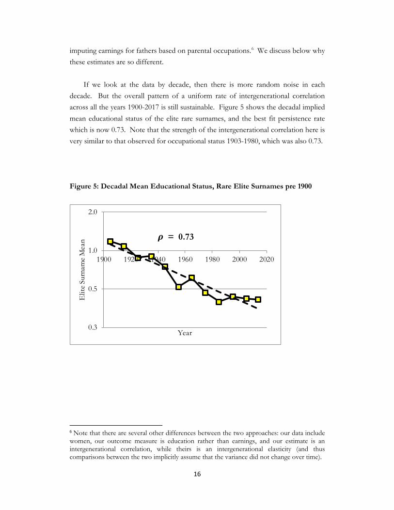
If we look at the data by decade, then there is more random noise in each decade. But the overall pattern of a uniform rate of intergenerational correlation across all the years 1900-2017 is still sustainable. Figure 5 shows the decadal implied mean educational status of the elite rare surnames, and the best fit persistence rate which is now 0.73. Note that the strength of the intergenerational correlation here is very similar to that observed for occupational status 1903-1980, which was also 0.73. Figure 5: Decadal Mean Educational Status, Rare Elite Surnames pre 1900

6 Note that there are several other differences between the two approaches: our data include women, our outcome measure is education rather than earnings, and our estimate is an intergenerational correlation, while theirs is an intergenerational elasticity (and thus comparisons between the two implicitly assume that the variance did not change over time).

0.3

0.5

1.0

2.0

1900 1920 1940 1960 1980 2000 2020

Elit

e Sur

nam

e Mea

n

Year

𝝆𝝆 = 0.73

17

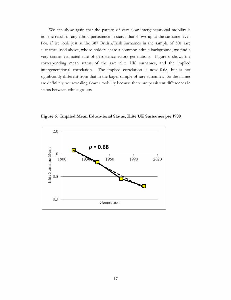
We can show again that the pattern of very slow intergenerational mobility is not the result of any ethnic persistence in status that shows up at the surname level. For, if we look just at the 387 British/Irish surnames in the sample of 501 rare surnames used above, whose holders share a common ethnic background, we find a very similar estimated rate of persistence across generations. Figure 6 shows the corresponding mean status of the rare elite UK surnames, and the implied intergenerational correlation. The implied correlation is now 0.68, but is not significantly different from that in the larger sample of rare surnames. So the names are definitely not revealing slower mobility because there are persistent differences in status between ethnic groups. Figure 6: Implied Mean Educational Status, Elite UK Surnames pre 1900

0.3

0.5

1.0

2.0

1900 1930 1960 1990 2020

Elit

e Sur

nam

e Mea

n

Generation

𝝆𝝆 = 0.68

18

As noted, there is evidence above in table 1 that the variance of occupational status among the elite rare surnames was greater than that for the population as a whole. For occupations this derives in part from the occupational status being skewed on all the three occupation measures, with more dispersal of attributed occupational status at the top of the social scale than at the bottom. Since the rare elite surnames are located on average towards the upper end of occupational status they will tend automatically to have a higher variance in occupational status than the population as a whole. Whether this translates into rarer surnames showing a greater variance in terms of educational attainment is not known. But we need to check that the intergenerational correlation estimates are robust to assumptions about the relative variance of educational status among elite surname holders and the population as a whole. In table 1, on the ANU2 occupational scale, the elite standard deviation is 1.40 times the population standard deviation for the stock of people aged 21+ in 1954, and 1.15 times in 1980. As a first robustness check we measure the implied intergenerational correlation implied by the relative representation at Melbourne and Sydney Universities, assuming the elite surname group has a standard deviation throughout which is 1.25 times that of the population. Figure 7 shows these results. The assumption of higher variance implies that the mean educational status of the elite surname holders in less in each period. But there is still a high implied correlation of status across generations. The estimated intergeneration correlation is still 0.65, compared to 0.70 which was the implied correlation with the assumption of equal educational status variances. However if the variance of the elite surname groups is approaching that of the general population as there is regression to the mean of this group, then in contrast the implied rate of social mobility declines compared to the base case. Thus if we keep the average elite surname group standard deviation 1.25 times that of the general population, but have its relative size decline by 4% each generation from 1.33 to 1.18 across the four generations 1900-2017, then now the implied intergenerational correlation becomes 0.75. Figure 8 shows the estimated mean status of the rare surnames under this alternative specification. Thus under any plausible specification the basic result of low rates of social mobility is robust.

19

Figure 7: Mean Educational Status, Elite Variance Higher than Population

Figure 8: Implied Mean Educational Status, Varying Elite Variance

0.13

0.25

0.50

1.00

2.00

1900 1930 1960 1990 2020

Elit

e Sur

nam

e Mea

n

Generation

𝝆𝝆 = 0.70

𝝆𝝆 = 𝟎𝟎.𝟔𝟕𝟕

0.13

0.25

0.50

1.00

2.00

1900 1930 1960 1990 2020

Elit

e Su

rnam

e M

ean

Generation

𝝆𝝆 = 0.70

𝝆𝝆 = 𝟎𝟎.𝟕𝟕𝟕𝟕

20

Since the end of World War II, the annual permanent migrant inflow into Australia has averaged 0.7 percent of the resident population – making Australia one of the most open countries to immigrants during this period. One issue that arises for an immigrant society such as Australia is the assumption that all holders of the rare elite surnames pre 1900 in 1900 and later were descended from the holders in Australia before 1900. Presumably some new immigrants with these surnames arrived after 1900. The effect of any such dilution, however, would be to reduce the observed intergenerational correlation below that which would truly hold for the surname members who were actual descendants of earlier Australian holders. However, only a small share of post-1960 Australian immigrants bore these rare surnames. If we look at the correlation between the numbers of voters with these surnames in 2014 and the number of people marrying with these surnames 1950-60 then that is 0.975. The random arrival of significant numbers of new immigrants with these surnames 1960-2014 would result in a significant decline in this correlation.

21

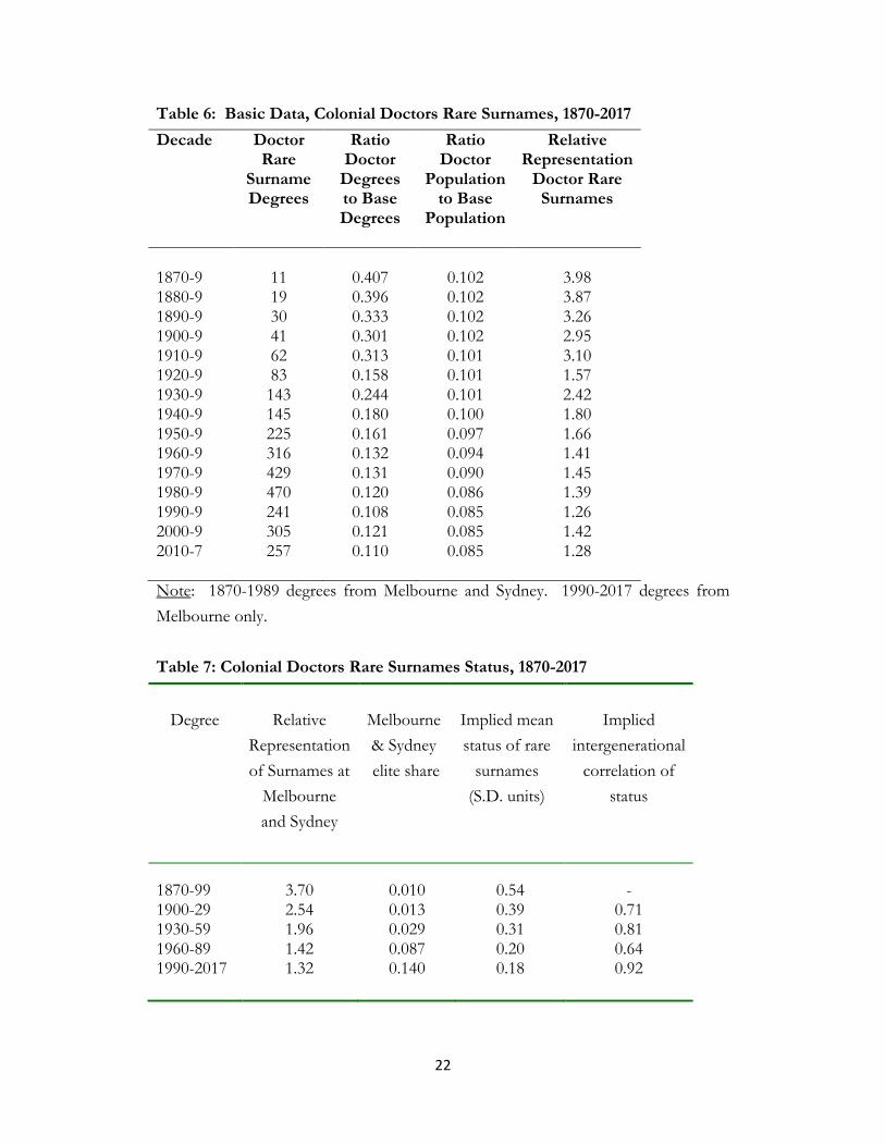
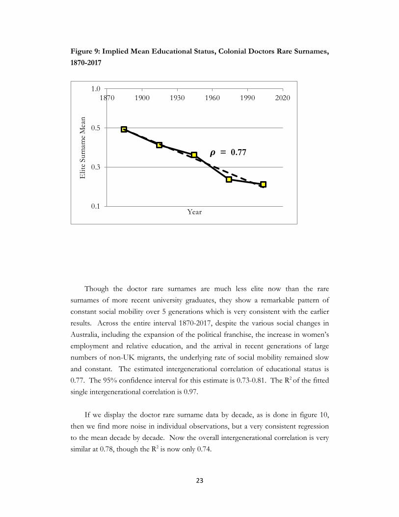
Rare Surnames, Early Doctors in Australia The Australian Medical Pioneers Index, available at the State Library of Victoria, provides biographical data on over 4,500 doctors who lived in Australia or visited Australia before 1875. The index includes those practicing medicine, as well as those who engaged in other occupations such as farming.7 The vast majority were doctors from the UK. The list includes, however, some doctors whose only contact with Australia was to make one or more return voyages on ships to Australia. Doctors in this era were not of as high a social status as now, but came from the middle of the social scale. Many were the sons of farmers, merchants, clergymen, or army and navy officers. But it does provide a list of a group of above average social status in colonial Australia. The average date of birth of these doctors is around 1823. Using again a cutoff of a frequency in the 2015 electoral roll of no more than 200, we find 1,018 rare surnames associated with this group. That makes a group of surnames twice as large as those with rare surnames getting degrees from Melbourne or Sydney universities 1870-1899. The average number of electors with one of these surnames in 2015 was 54. Table 6 shows the basic data for this group in terms of degree recipients from Melbourne and Sydney universities. From 1870 on holders of these names were more likely than holders of large frequency UK surnames to receive university degrees. Before 1900 they were nearly four times as likely to receive a degree, but their overrepresentation steadily declined. Table 7 shows the calculated average educational status of this group of surnames by generation 1870-2017. Figure 9 plots this implied mean educational status and shows the fitted intergenerational correlation across the five generations, which is 0.77.

7 The index was compiled by Dr. Noel David Richards.

22

Table 6: Basic Data, Colonial Doctors Rare Surnames, 1870-2017 Decade Doctor

Rare Surname Degrees

Ratio Doctor

Degrees to Base Degrees

Ratio Doctor

Population to Base

Population

Relative Representation

Doctor Rare Surnames

1870-9 11 0.407 0.102 3.98 1880-9 19 0.396 0.102 3.87 1890-9 30 0.333 0.102 3.26 1900-9 41 0.301 0.102 2.95 1910-9 62 0.313 0.101 3.10 1920-9 83 0.158 0.101 1.57 1930-9 143 0.244 0.101 2.42 1940-9 145 0.180 0.100 1.80 1950-9 225 0.161 0.097 1.66 1960-9 316 0.132 0.094 1.41 1970-9 429 0.131 0.090 1.45 1980-9 470 0.120 0.086 1.39 1990-9 241 0.108 0.085 1.26 2000-9 305 0.121 0.085 1.42 2010-7 257 0.110 0.085 1.28 Note: 1870-1989 degrees from Melbourne and Sydney. 1990-2017 degrees from Melbourne only. Table 7: Colonial Doctors Rare Surnames Status, 1870-2017

Degree

Relative

Representation of Surnames at

Melbourne and Sydney

Melbourne & Sydney elite share

Implied mean status of rare

surnames (S.D. units)

Implied

intergenerational correlation of

status

1870-99 3.70 0.010 0.54 - 1900-29 2.54 0.013 0.39 0.71 1930-59 1.96 0.029 0.31 0.81 1960-89 1.42 0.087 0.20 0.64 1990-2017 1.32 0.140 0.18 0.92

23

Figure 9: Implied Mean Educational Status, Colonial Doctors Rare Surnames, 1870-2017

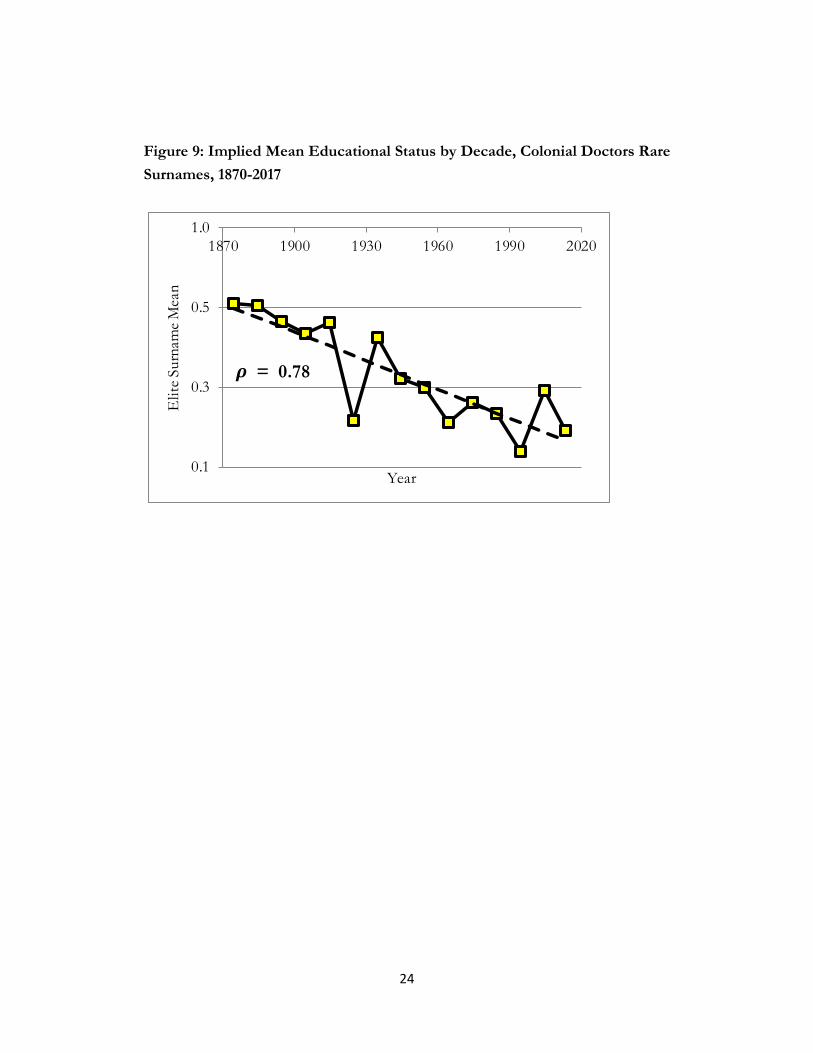
Though the doctor rare surnames are much less elite now than the rare surnames of more recent university graduates, they show a remarkable pattern of constant social mobility over 5 generations which is very consistent with the earlier results. Across the entire interval 1870-2017, despite the various social changes in Australia, including the expansion of the political franchise, the increase in women’s employment and relative education, and the arrival in recent generations of large numbers of non-UK migrants, the underlying rate of social mobility remained slow and constant. The estimated intergenerational correlation of educational status is 0.77. The 95% confidence interval for this estimate is 0.73-0.81. The R2 of the fitted single intergenerational correlation is 0.97. If we display the doctor rare surname data by decade, as is done in figure 10, then we find more noise in individual observations, but a very consistent regression to the mean decade by decade. Now the overall intergenerational correlation is very similar at 0.78, though the R2 is now only 0.74.

0.1

0.3

0.5

1.01870 1900 1930 1960 1990 2020

Elit

e Sur

nam

e Mea

n

Year

𝝆𝝆 = 0.77

24

Figure 9: Implied Mean Educational Status by Decade, Colonial Doctors Rare Surnames, 1870-2017

0.1

0.3

0.5

1.01870 1900 1930 1960 1990 2020

Elit

e Sur

nam

e Mea

n

Year

𝝆𝝆 = 0.78

25

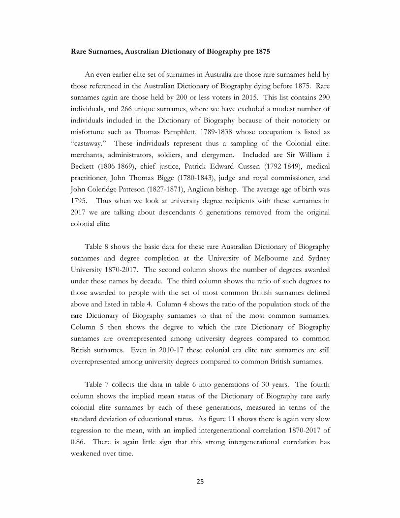
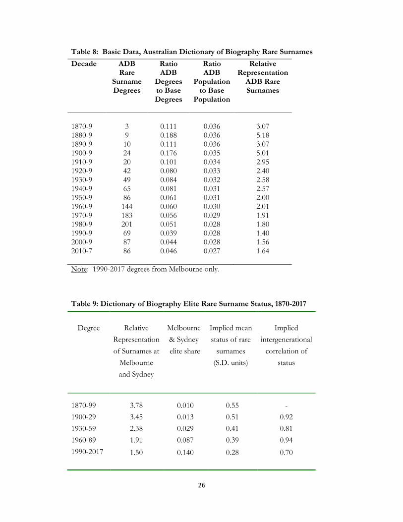
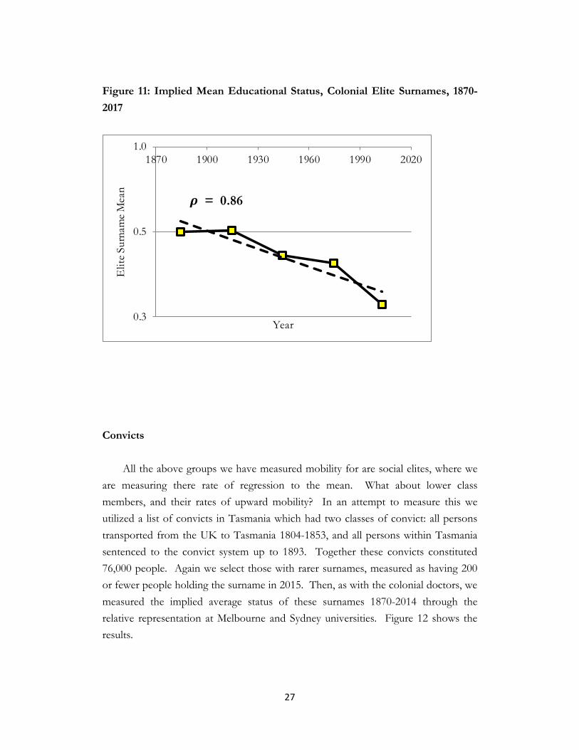
Rare Surnames, Australian Dictionary of Biography pre 1875 An even earlier elite set of surnames in Australia are those rare surnames held by those referenced in the Australian Dictionary of Biography dying before 1875. Rare surnames again are those held by 200 or less voters in 2015. This list contains 290 individuals, and 266 unique surnames, where we have excluded a modest number of individuals included in the Dictionary of Biography because of their notoriety or misfortune such as Thomas Pamphlett, 1789-1838 whose occupation is listed as “castaway.” These individuals represent thus a sampling of the Colonial elite: merchants, administrators, soldiers, and clergymen. Included are Sir William à Beckett (1806-1869), chief justice, Patrick Edward Cussen (1792-1849), medical practitioner, John Thomas Bigge (1780-1843), judge and royal commissioner, and John Coleridge Patteson (1827-1871), Anglican bishop. The average age of birth was 1795. Thus when we look at university degree recipients with these surnames in 2017 we are talking about descendants 6 generations removed from the original colonial elite. Table 8 shows the basic data for these rare Australian Dictionary of Biography surnames and degree completion at the University of Melbourne and Sydney University 1870-2017. The second column shows the number of degrees awarded under these names by decade. The third column shows the ratio of such degrees to those awarded to people with the set of most common British surnames defined above and listed in table 4. Column 4 shows the ratio of the population stock of the rare Dictionary of Biography surnames to that of the most common surnames. Column 5 then shows the degree to which the rare Dictionary of Biography surnames are overrepresented among university degrees compared to common British surnames. Even in 2010-17 these colonial era elite rare surnames are still overrepresented among university degrees compared to common British surnames. Table 7 collects the data in table 6 into generations of 30 years. The fourth column shows the implied mean status of the Dictionary of Biography rare early colonial elite surnames by each of these generations, measured in terms of the standard deviation of educational status. As figure 11 shows there is again very slow regression to the mean, with an implied intergenerational correlation 1870-2017 of 0.86. There is again little sign that this strong intergenerational correlation has weakened over time.

26

Table 8: Basic Data, Australian Dictionary of Biography Rare Surnames Decade ADB

Rare Surname Degrees

Ratio ADB

Degrees to Base Degrees

Ratio ADB

Population to Base

Population

Relative Representation

ADB Rare Surnames

1870-9 3 0.111 0.036 3.07 1880-9 9 0.188 0.036 5.18 1890-9 10 0.111 0.036 3.07 1900-9 24 0.176 0.035 5.01 1910-9 20 0.101 0.034 2.95 1920-9 42 0.080 0.033 2.40 1930-9 49 0.084 0.032 2.58 1940-9 65 0.081 0.031 2.57 1950-9 86 0.061 0.031 2.00 1960-9 144 0.060 0.030 2.01 1970-9 183 0.056 0.029 1.91 1980-9 201 0.051 0.028 1.80 1990-9 69 0.039 0.028 1.40 2000-9 87 0.044 0.028 1.56 2010-7 86 0.046 0.027 1.64 Note: 1990-2017 degrees from Melbourne only. Table 9: Dictionary of Biography Elite Rare Surname Status, 1870-2017

Degree

Relative

Representation of Surnames at

Melbourne and Sydney

Melbourne & Sydney elite share

Implied mean status of rare

surnames (S.D. units)

Implied

intergenerational correlation of

status

1870-99 3.78 0.010 0.55 - 1900-29 3.45 0.013 0.51 0.92 1930-59 2.38 0.029 0.41 0.81 1960-89 1.91 0.087 0.39 0.94 1990-2017 1.50 0.140 0.28 0.70

27

Figure 11: Implied Mean Educational Status, Colonial Elite Surnames, 1870-2017

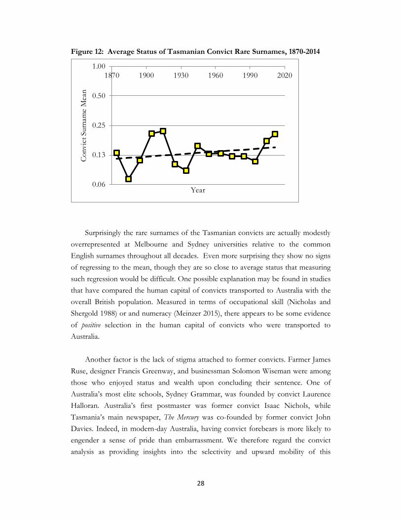
Convicts All the above groups we have measured mobility for are social elites, where we are measuring there rate of regression to the mean. What about lower class members, and their rates of upward mobility? In an attempt to measure this we utilized a list of convicts in Tasmania which had two classes of convict: all persons transported from the UK to Tasmania 1804-1853, and all persons within Tasmania sentenced to the convict system up to 1893. Together these convicts constituted 76,000 people. Again we select those with rarer surnames, measured as having 200 or fewer people holding the surname in 2015. Then, as with the colonial doctors, we measured the implied average status of these surnames 1870-2014 through the relative representation at Melbourne and Sydney universities. Figure 12 shows the results.

0.3

0.5

1.01870 1900 1930 1960 1990 2020

Elit

e Sur

nam

e Mea

n

Year

𝝆𝝆 = 0.86

28

Figure 12: Average Status of Tasmanian Convict Rare Surnames, 1870-2014

Surprisingly the rare surnames of the Tasmanian convicts are actually modestly overrepresented at Melbourne and Sydney universities relative to the common English surnames throughout all decades. Even more surprising they show no signs of regressing to the mean, though they are so close to average status that measuring such regression would be difficult. One possible explanation may be found in studies that have compared the human capital of convicts transported to Australia with the overall British population. Measured in terms of occupational skill (Nicholas and Shergold 1988) or and numeracy (Meinzer 2015), there appears to be some evidence of positive selection in the human capital of convicts who were transported to Australia.

Another factor is the lack of stigma attached to former convicts. Farmer James Ruse, designer Francis Greenway, and businessman Solomon Wiseman were among those who enjoyed status and wealth upon concluding their sentence. One of Australia’s most elite schools, Sydney Grammar, was founded by convict Laurence Halloran. Australia’s first postmaster was former convict Isaac Nichols, while Tasmania’s main newspaper, The Mercury was co-founded by former convict John Davies. Indeed, in modern-day Australia, having convict forebears is more likely to engender a sense of pride than embarrassment. We therefore regard the convict analysis as providing insights into the selectivity and upward mobility of this

0.06

0.13

0.25

0.50

1.001870 1900 1930 1960 1990 2020

Conv

ict S

urna

me

Mea

n

Year

29

particular group, but not to the broader question of long-run intergenerational mobility in Australia. Interpretation

There is a long-held pride among Australians about living in a fluid society, where Jack isn’t just as good as his master, but perhaps better. Relative to national income, the all-time richest-ever Australian was probably Samuel Terry, who was sent as a convict to Australia for stealing stockings. The man known as ‘The Botany Bay Rothschild’ died in 1838 with an estate equivalent to around 4 percent of GDP in that year.8 As Charles Darwin wrote in his diary when he visited in the 1830s, Australians of that era seemed to believe that anyone could strike it rich: ‘The whole population, poor and rich, are bent on acquiring wealth: amongst the highest orders, wool and sheep-grazing form the constant subject of conversation.’ (Darwin 1845, 444). In the 1960s, McGregor (1966, 110) argued of Australia that: ‘There is not so much difference between the way the different classes speak, the way they dress or the schools they went to as in England, which makes it easier for individuals to move from social group to group. … The lack of widespread extremes in social differentiation makes it easy for class-jumpers to “pass”.’

A belief in social mobility has accompanied a pride in Australian egalitarianism.

In World War One, off-duty Australian soldiers refused to salute British officers. Some briefly went on strike. Soldiers prize the epithet ‘digger’, citizens often call one another ‘mate’. Australians rarely stand when the Prime Minister enters the room, and often ride in the front seat of taxis.

Institutionally, the design of the Australian social safety net should improve

social mobility. As Whiteford (2010) points out, Australia has a higher share of spending on income-tested programs than any other OECD country. A dollar spent in the Australian social security system is more targeted to low-income recipients than in any other advanced nation. This is not a new phenomenon: for example, the Australian age pension has been means-tested since the 1930s (Leigh 2013).

8 Terry’s estate was worth £250,000 (Dow 1967), and Australian GDP for 1838 has been estimated at £5.9 million (Butlin 1985, Table 1).

30

The popular belief in a socially open and mobile Australia had seemed to find support in academic studies of social mobility in recent years. In an ideal world, researchers estimating intergenerational mobility draw upon multiple years of income data for parents and children. This typically requires matched social security records, matched taxation records, or a long-running panel survey. To date, these have not been available for Australia. The main longitudinal survey only commenced in 2001, and efforts to match taxation or social security records across generations data have not yet borne fruit. In the absence of these ideal sources, researchers have therefore fallen back on the alternative approach of imputing parental incomes using parents’ occupations. Leigh (2007) estimated an intergenerational elasticity for fathers and sons in the range of 0.2 to 0.3, a figure that did not appear to have changed much in the preceding four decades. Using considerably more data, Mendolia and Siminski (2016) re-estimated the modern-day intergenerational earnings elasticity at 0.35, which stands as the benchmark estimate for Australia.

An international comparison of mobility (Corak, 2013) puts the

intergenerational income elasticity for Britain and the United States each at around 0.5. Comparing across countries, this suggests that on conventional metrics, Australia is a more socially mobile society than Britain – its old colonial power or the United States – the world’s largest advanced nation.

Yet the surname estimates above suggest that Australia shows strong status

persistence across multiple generations. The great-great-great-great grandchildren of the medical pioneers in Australia graduating from university after 2010, six generations later, show an implied educational status that is still about 0.2 standard deviations above the mean for descendants of UK immigrants. The underlying correlation of social status is 0.7-0.8. That correlation is as high now as in the 1870s. There was no increase in social mobility over the years 1870-2017. That correlation is also as high as in England and in the USA.

How do we reconcile these very different pictures of Australian society?

Interestingly in the first section above we look at occupational status 1903-1980, while the current intergenerational income elasticities for Australia are also estimated using occupations to infer incomes. In this sense, the approaches rely on similar data.

31

One issue here is that the estimated persistence rates for earnings in Australia, which have to depend on attributing earnings through occupations, are likely biased downwards compared to estimates which rely on actual earnings estimates for parent and child. The correlation between occupational status and average earnings by occupation in a country like Australia is actually modest: for the recent occupational status scale AUSE106 and earnings in 2016 the correlation was only 0.58.9 Occupations thus provide a noisy measure of earnings, and any such noise will reduce intergenerational elasticities.10 In contrast the surname-based estimates are not affected by these issues of noise in earnings or occupational status attribution. Thus Australia may not have such high rates of income mobility compared to England and the USA as the coefficient estimates would suggest.

But even if we could measure earnings or occupational status perfectly, we

would still likely observe that the correlation of parent and child is lower than the underlying correlation observed across generations. This is because there is plenty of evidence that the pattern of social mobility is best captured by the model described in equations (1) and (2) above. Underlying status is transmitted strongly across generations, but within each generation there is a random component linking underlying status and the actual achieved status of a person. With such a structure the correlation between parent and child in social status is always lower than the correlation that described mobility across multiple generations. There is no longer any unitary measure of social mobility rates. You can have low rates of persistence of status comparing parent and child, but still very strong persistence at the level of family lineages or social classes.

9 For AUSE106 see McMillan et al., 2009. 10 Both Leigh (2007) and Mendolia and Siminski (2016) adjust for this problem by also running their occupation-based technique on US data, then taking benchmark income-based intergenerational elasticities from the US literature (eg Solon 1992; Mazumder 2005) to derive a measure of the downward bias of the methodology. This bias estimate is then used to scale up the Australian estimate. However, the reliability of this approach turns on the accuracy of published estimates of the US intergenerational elasticity. If the benchmark US intergenerational elasticity estimates are too low, then using them to correct for bias in the Australian studies will produce an underestimate estimate of the Australian intergenerational elasticity. Finally, it is worth noting Huang, Perales and Western (2016), a study in the sociology literature that makes no correction for the downward bias inherent in using occupations to impute earnings, and therefore produces a higher estimate of Australian intergenerational mobility than Mendolia and Siminski (2016).

32

With this structure the social system behaves as though it has a longer memory of family status. The predicted status of children depends not just on the parents, but also on the grandparents, uncles, aunts and other relatives. In high status lineages, large short-term declines in status by a child tend to be corrected in the next generation, the grandchildren. For lower class families large upward movements in social status tend also to get corrected in the next generation.

Another feature that should be emphasized is that our data does suggest there

will be complete social mobility in Australia, if we wait enough generations. The descendants of the Colonial elite are becoming more average with each passing generation, and will eventually be completely average in status. However, this process takes a very long time. The holders of rare elite surnames in table 2 had an average occupational status 1.54 standard deviations above the social mean in 1904. With an intergenerational correlation of 0.75 in occupational status their average status will lie within .1 standard deviations of the social mean by the generation of 2204. It takes about 10 generations, 300 years, for such an elite set of families to become effectively average.

It is not obvious how we should weight the two different elements of short run

and long run mobility in terms of evaluating the degree of social mobility in Australian society. Indeed, policies that increase parent-child social mobility may be desirable even if we expect that there will be some reversion in the next generation. But it is clear that in terms of long-run social mobility, Australia has been just as immobile a society as its sclerotic parent England.

33

Sources Electoral Rolls 1903-1980 from ancestry.com Marriage Index, 1788-1950 (surname frequencies 1870-1950) from ancestry.com Australian Medical Pioneers Index from medicalpioneers.com Melbourne University Graduates, 1856-2017, supplied by Melbourne University Sydney University Graduates, 1853-1985 from alumniarchives.sydney.edu.au/as/

The Intellectual Property Agency of the Australian Government maintains a searchable database of surname frequencies in Australia, based on the electoral register. Australian Government, “Search for Australian Surnames,” pericles.ipaustralia.gov.au/atmoss/falcon_search_tools.Main?pSearch=Surname. This site can be searched for any string of letters in a surname. In 2012 there were 14.3 million enrolled electors in Australia, representing 90 percent of all adults. Because of the enrollment requirement, there is a tendency for this site to undercount lower-status surnames.

34

References

Broom, L., F.L. Jones, P. Duncan-Jones, and P. McDonnell. 1977. "Status scores for all Australian occupations", pp. 58-111 in Broom et al., Investigating Social Mobility, Department of Sociology RSSS, Monograph No. 1, Canberra: ANUTECH, Australian National University.

Butlin, Noel. 1985. “Australian National Accounts 1788-1983” Source Papers in Economic History Number 6, Australian National University, Canberra.

Chetty, Raj, Nathaniel Hendren, Patrick Kline, Emmanuel Saez, and Nick Turner. 2014a. “Is the United States Still a Land of Opportunity? Recent Trends in Intergenerational Mobility”, NBER Working Paper No. 19844, Cambridge, MA: NBER.

Chetty, Raj, Nathaniel Hendren, Patrick Kline, Emmanuel Saez, and Nick Turner. 2014b. “Is the United States Still a Land of Opportunity? Recent Trends in Intergenerational Mobility”, American Economic Review 104(5): 141-147.

Clark, Gregory, Neil Cummins, Max Hua, Dan Diaz Vidal et al. 2014. The Son Also Rises: Surnames and the History of Social Mobility. Princeton: Princeton University Press.

Clark, Gregory and Neil Cummins. 2015. “Intergenerational Wealth Mobility in England, 1858-2012. Surnames and Social Mobility.” Economic Journal, 125(582): 61-85.

Clark, Gregory and Daniel Diaz Vidal. 2017. “Why is Surname Status Persistence so Strong? Social Group or Dynastic Transmission versus Family Effects.” Working Paper.

Corak, Miles. 2013. “Income inequality, equality of opportunity, and intergenerational mobility”. Journal of Economic Perspectives, 27(3), pp.79-102.

Darwin, Charles. 1845. Journal of researches into the natural history and geology of the countries visited during the voyage of H.M.S. Beagle round the world, under the Command of Capt. Fitz Roy, R.N. (Second ed.), London: John Murray..

Dow, Gwyneth. 1967. “Terry, Samuel (1776–1838)”, Australian Dictionary of Biography, Vol 2. National Centre of Biography, Australian National University, Canberra.

Huang, Yangtao, Perales, Francisco, and Mark Western. 2016. “A land of the ‘fair go’? Intergenerational earnings elasticity in Australia.” Australian Journal of Social Issues, 51(3): 361–381.

Jones, F. Lancaster. 1989. "Occupational Prestige in Australia: a New Scale", Australian and New Zealand Journal of Sociology, 25(2): 187-199.

35

Krueger, Alan. 2012. The rise and consequences of inequality. Presentation made to the Center for American Progress, January 12th.

Leigh, Andrew. 2007. “Intergenerational Mobility in Australia.” The B.E. Journal of Economic Policy and Analysis. Contributions. Vol. 7(2), Article 6.

Leigh, Andrew. 2013. Battlers and Billionaires: The Story of Inequality in Australia, Black Inc, Melbourne.

Mazumder, B., 2005. “Fortunate sons: New estimates of intergenerational mobility in the United States using social security earnings data”. Review of Economics and Statistics, 87(2), pp.235-255.

McGregor, Craig. 1966. Profile of Australia, Hodder and Stoughton, London. McMillan, Julie and F. L. Jones. 2000. “The ANU3_2 scale: a revised occupational

status scale for Australia.” Journal of Sociology, 36(1): 64-80. McMillan, Julie, Adrian Beavis, & Frank L. Jones, (2009) 'The AUSEI06: A new

socioeconomic index for Australia' Journal of Sociology. Vol 45(2): 123-149. Meinzer, Nicholas J. 2015. “The Western Australian Convicts”, Australian Economic

History Review, 55(2): 163-186. Mendolia, Silvia and Peter Siminski. 2016. “New Estimates of Intergenerational

Mobility in Australia”, Economic Record, 92(298): 361–373. Nicholas, Stephen and Peter R. Shergold. 1988. 'Convicts as Workers' in Stephen

Nicholas (ed.) Convict Workers: Reinterpreting Australia's Past, Cambridge University Press, Cambridge, pp. 62-84.

Solon, G. 1992. “Intergenerational Income Mobility in the United States”, American Economic Review, 82(3), 393–408.

Torche, Florencia and Alejandro Corvalan. 2016. “Estimating Intergenerational Mobility With Grouped Data: A Critique of Clark’s The Son Also Rises.” Sociological Methods & Research.

Universities Admissions Centre. 2015. “Calculating the Australian Tertiary Admission Rank in New South Wales: A Technical Report”, Universities Admissions Centre, Sydney.

Whiteford, P., 2010. “The Australian Tax‐Transfer System: Architecture and Outcomes”. Economic Record, 86(275): 528-544.

36

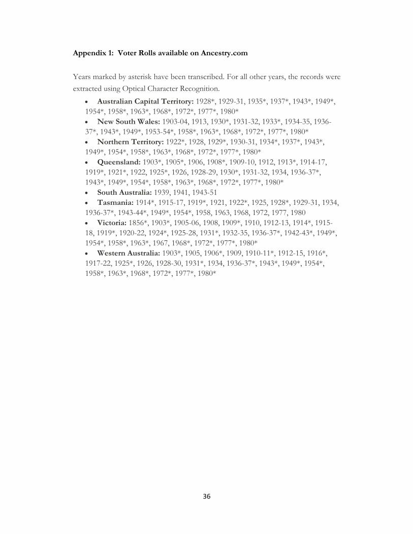
Appendix 1: Voter Rolls available on Ancestry.com Years marked by asterisk have been transcribed. For all other years, the records were extracted using Optical Character Recognition.

• Australian Capital Territory: 1928*, 1929-31, 1935*, 1937*, 1943*, 1949*, 1954*, 1958*, 1963*, 1968*, 1972*, 1977*, 1980* • New South Wales: 1903-04, 1913, 1930*, 1931-32, 1933*, 1934-35, 1936-37*, 1943*, 1949*, 1953-54*, 1958*, 1963*, 1968*, 1972*, 1977*, 1980* • Northern Territory: 1922*, 1928, 1929*, 1930-31, 1934*, 1937*, 1943*, 1949*, 1954*, 1958*, 1963*, 1968*, 1972*, 1977*, 1980* • Queensland: 1903*, 1905*, 1906, 1908*, 1909-10, 1912, 1913*, 1914-17, 1919*, 1921*, 1922, 1925*, 1926, 1928-29, 1930*, 1931-32, 1934, 1936-37*, 1943*, 1949*, 1954*, 1958*, 1963*, 1968*, 1972*, 1977*, 1980* • South Australia: 1939, 1941, 1943-51 • Tasmania: 1914*, 1915-17, 1919*, 1921, 1922*, 1925, 1928*, 1929-31, 1934, 1936-37*, 1943-44*, 1949*, 1954*, 1958, 1963, 1968, 1972, 1977, 1980 • Victoria: 1856*, 1903*, 1905-06, 1908, 1909*, 1910, 1912-13, 1914*, 1915-18, 1919*, 1920-22, 1924*, 1925-28, 1931*, 1932-35, 1936-37*, 1942-43*, 1949*, 1954*, 1958*, 1963*, 1967, 1968*, 1972*, 1977*, 1980* • Western Australia: 1903*, 1905, 1906*, 1909, 1910-11*, 1912-15, 1916*, 1917-22, 1925*, 1926, 1928-30, 1931*, 1934, 1936-37*, 1943*, 1949*, 1954*, 1958*, 1963*, 1968*, 1972*, 1977*, 1980*