NBER WORKING PAPER SERIES

IMMIGRATION, HUMAN CAPITAL FORMATION AND ENDOGENOUS ECONOMICGROWTH

Isaac EhrlichJinyoung Kim

Working Paper 21699http://www.nber.org/papers/w21699

NATIONAL BUREAU OF ECONOMIC RESEARCH1050 Massachusetts Avenue

Cambridge, MA 02138November 2015

A preliminary version of this paper was presented in the IZA/UB Center for Human Capital Workshopon Migration and Human Capital held in Bonn on May 23-24, 2013. A more recent version was presentedin the conference honoring the life and work of Gary Becker at the Becker-Friedman Institute in Chicagoon October 16, 2015. We are indebted to participants in both conferences for valuable comments. Wealso wish to acknowledge very helpful comments and suggestions by Yong Yin and James Smith,editorial assistance by Chaya Ehrlich, and research assistance by Bibaswan Chatterjee, Soomin Lee,Minsung Park and Po-Chieh Yang. The views expressed herein are those of the authors and do notnecessarily reflect the views of the National Bureau of Economic Research.

NBER working papers are circulated for discussion and comment purposes. They have not been peer-reviewed or been subject to the review by the NBER Board of Directors that accompanies officialNBER publications.

© 2015 by Isaac Ehrlich and Jinyoung Kim. All rights reserved. Short sections of text, not to exceedtwo paragraphs, may be quoted without explicit permission provided that full credit, including © notice,is given to the source.

Immigration, Human Capital Formation and Endogenous Economic GrowthIsaac Ehrlich and Jinyoung KimNBER Working Paper No. 21699November 2015, Revised December 2015JEL No. F22,F43,O15,O4

ABSTRACT

Census data from international sources covering 77% of the world’s migrant population indicate thatthe skill composition of migrants in major destination countries, including the US, has been risingover the last 4 decades. Moreover, the population share of skilled migrants has been approaching orexceeding that of skilled natives. We offer theoretical propositions and empirical tests consistent withthese trends via a general-equilibrium model of endogenous growth where human capital, population,income growth and distribution, and migration trends are endogenous. We derive new insights aboutthe impact of migration on long-term income growth and distribution, and the net benefits to nativesin both destination and source countries.

Isaac Ehrlich415 Fronczak HallState University of New York at Buffaloand Center for Human CapitalBox 601520Buffalo, NY 14260-1520and NBERmgtehrl@buffalo.edu

Jinyoung KimDepartment of EconomicsKorea University5-1, Anam-Dong, Sungbuk-KuSeoul, Korea 136-701jinykim@korea.ac.kr

1

I. Introduction

Over the last four decades, the five major receiving countries – the US, UK, France, Australia and

Canada – have experienced a surge in net migration flows along with a significant rise in the proportion

of high-skilled migrants age 25+, which we define empirically in this paper as population groups with at

least some college education (i.e., 13+ years of schooling) or degrees.1 This evidence comes from 2

international panels: one by the World Bank, including data from 1975-2000, which we use in our

empirical investigation in section VII of this paper, and another by the Institute of Employment Research

in Germany (IAB) including supplementary data from 1980-2010, which we use to illustrate the

continuing trend. Moreover, data taken from Barro and Lee (2013) indicate that in most of these

destination countries the proportion of skilled migrants has actually caught up with or exceeded the

proportion of high-skilled total populations in the corresponding destination countries, and thus clearly

the proportion of natives as well. (See figure 1).

These trends have been less pronounced in the US over the same period because of the bimodal

distribution of the educational attainments of migrants to the US. Still, the upward trends in the high-

skilled composition of the migrant population in the US have been similar to those of the other four

receiving countries, and the Census of Population data for the US show that the proportion of migrants

entering the US over the period 2000-2012 with more than a BA degree has just exceeded the

corresponding proportion of natives. These trends are sharper among migrants from Asia and Europe, or

‘Other’ countries, especially in the case of migrants with MA degrees and over and those with PhD

degrees, relative to US natives - see Figures 2 and 3. Our main objective in this paper is to explain the

pattern of migration and its skill composition over transitional dynamic periods that are triggered by

significant shifts in underlying exogenous parameters, and to assess their impact on long-term income

growth and distribution in both destination and source countries, including the long-term net benefits to

the native populations in both countries, using a dynamic general equilibrium approach.

We pursue these issues via an open economy, overlapping generations, endogenous growth model in

which population and immigration are also endogenous, labor is mobile internationally, and human

capital is both the engine of growth and the main determinant of income distribution. The current open-

economy model is largely an extension of earlier work by us (Ehrlich and Kim [EK], 2007) which

focused on the dynamics of income growth and income distribution in a closed economy setting.2

1 Germany belongs in this set as well, but the time series for Germany is problematic because of the division between East and West up to 1990, so we have not included it in our work using the WB panel data. 2 An earlier attempt to develop such extension has been made in the dissertation work of Idu (2012).

2

There is an extensive literature that has analyzed related issues using a neoclassical macro-

equilibrium setting which allows for migration by homogeneous or heterogeneous skills and short-term

physical capital adjustments to migration shocks. A more recent literature which is more relevant for our

model (see section II) focuses on the long term, persisting consequences of migration using endogenous

growth paradigms where the engine of growth is either technological or human capital investments.

Common to both strands of the extant literature is the treatment of migration as an exogenous variable.

The distinct feature of our paper is its attempt to consider how immigration, when treated as an

endogenous variable, interacts with income growth and income distribution within and across both

sending and receiving countries in a balanced-growth global equilibrium regime. To fully endogenize

immigration, we formally link both receiving and sending countries and allow for more than one type of

human capital in both.

In both our 2007 paper and the current study human capital investment decisions originate at the

individual level of heterogeneous households. Parents of different skill types determine both the quantity

and education or human capital attainments of their offspring, and human capital formation is influenced

by knowledge spillover effects flowing from parents to children within households, as well as across

workers with different skills. This assumption is generalized in this paper by allowing for intra-

generational knowledge spillover effects from higher to lower skill groups, which include both natives

and immigrants, within receiving and sending countries and across these countries. Workers of different

skills can choose to migrate from home to destination countries in response to differences in technological

and cost parameters affecting the net returns to migration.

A calibrated simulation of the model yields a global, balanced growth equilibrium steady state in

which: (i) the growth rates in population and human capital are constant and ultimately equalize across

countries and within skilled groups in each country, including migrants; and (ii) a constant fraction of

each population group in the source country migrates to the destination country. The model can also trace

the trends in these variables over transitional dynamic phases, triggered by exogenous shocks in the

model’s basic parameters. The emerging patterns of migration, growth, and income inequality, and their

impact on the ultimate net benefits of migration to the receiving and sending countries, generally depends,

however, on the specific exogenous shock representing “pull” or “push” factors, and the country in which

it first occurs.

Our working assumption is that the general pattern of migration in recent decades has been induced

by the “pull” force of a skill-biased technological advance occurring in the receiving country, or in both

the receiving and sending countries simultaneously, such as the hi-tech Internet revolution of the early

3

1970s. Our numerical analysis implies that such a shift generates a higher rate of human capital formation

and per-capita income growth, and a generally rising level and share of skilled migrants relative to both

the migrant and native populations in the receiving countries. The latter implications are also tested

through a regression analysis using a World Bank panel of 190 countries over the period 1975-2000. Our

analysis enables us to derive new insights about the long-term, self-sustaining net gains from immigration

to both destination and source countries, and compare them to the “immigration surplus” as assessed by

the earlier literature.

The structure of the paper is as follows: In section II we review some of the literature that is more

relevant for our model. In section III we introduce the benchmark version of our model that treats

immigrants and natives as separate factors of knowledge production and in section IV we solve this model

via calibrated numerical analysis. In section V we likewise introduce and solve the extended version of

the model that allows for “diversity effects” in knowledge production, and in section VI we use both

models to estimate the long-term consequences of immigration on the net welfare of natives. In section

VII we test the basic propositions of the model empirically. We conclude with a summary of the overall

insights offered by our study about the long-term impact of immigration on both source and destination

countries.

II. Related Literature

The skill composition of migrants and its relevance for income growth and inequality have also been

analyzed in previous literature using a neo-classical growth setting or an endogenous growth approach.

We here review some of the papers with direct relevance to our model.

A. Macro models tested against empirical data

On the relation between income inequality and skilled migration: Borjas (1987) models the migration

decision to be a function of the differential rate of return on skill. He argues that a destination country that

has a higher rate of return (ROR) on skill than a source country tends to attract skilled workers. Using

income inequality as proxy for relative ROR for skill he concludes that income inequality in a destination

country should be positively correlated with a larger proportion of skilled migrants, while income

inequality in a source country should be negatively correlated with the skill composition of migrants.

Clark, Hatton, and Williamson (2007) find that a 10% increase in sending-country inequality, evaluated at

its mean, lower the volume of immigration by 7.5%. Kahanec-Zimmerman (2008) find, however, that the

quality of immigration to OECD economies is negatively related to income inequality in destination. In

4

Brucker, Defoort (2007), in contrast, the ratio of skilled to unskilled migrants and the Gini coefficients of

both sending and receiving countries, are positively related. The inconsistent evidence may be partly

rationalized by the fact that income inequality is treated as an exogenous variable in the previous studies.

By our approach the relationship between skill composition of migrants and income inequality is

associative, not causal, since both are simultaneously determined.

On the determinants of the skill composition of migrants: Most studies find that skilled emigrants tend to

move first in response to incentives to migrate, followed by unskilled emigrants because of a diaspora

effect charting an inverted-U time path of skill composition. Hatton-Williamson (2004) argue that skilled

workers are first to emigrate because they can afford high migration and settlement costs. As migrant

networks are established, however, unskilled worker find it easier to migrate later. This general pattern is

confirmed by our comparative dynamics predictions as well.

B. Endogenous growth models

The endogenous growth literature has generally identified two main engines of growth and related

paradigms that can generate persistent and self-sustaining growth in factor productivity and thus in per-

capita income growth over the long haul: human capital formation, and induced technological innovations.

The first paradigm places the focus on investments in human knowledge and health, cognitive skills and

higher education, along with other determinants of human capital (fertility, health, population size), as

driven by individuals and families investing in their own or their offspring’s education and training. The

second approach places the focus on technological innovations as driven by profit maximizing firms

investing in R&D and competing over innovations involving higher quality products and production

processes or greater variety and superior quality of new goods which expand real output and welfare.

Each approach recognizes, however, the independent role of the alternative factor, but takes it to be

exogenously shifting. Each paradigm also places an emphasis on the role of external economies or

spillover effects which are essential for establishing long-term balanced growth equilibrium paths and

associated income distributions in economies with heterogeneous agents or goods.

There is a large literature associated with each paradigm based largely on closed-economy settings.3

There is also, however, a nascent literature which has sought to study the role of immigration within

endogenous growth models based explicitly or implicitly on open economy settings. This literature has

also bifurcated along the same lines of the earlier literature by adopting either induced technology or

human capital formation as the major engines of growth. In this section we briefly discuss and compare

3 For example, Lucas (1988), Romer (1990), Becker, Murphy and Tamura (1990), Ehrlich and Lui (1991), Stokey (1988), Galor and Moav (2004), and Ehrlich and Kim (2007).

5

the mechanics, main propositions, and general welfare implications offered in a few selected papers

representing each approach in the literature.

1. Immigration and R&D externalities:

The product-innovation-based models focus on the potential contribution of immigrants to the scale

of the labor force employed in the R&D sector of the economy through various channels. For example,

Lundborg and Segestrom [LS] (2000, 2002) develop two versions of an open economy model with two

trading countries (North-North, or North-South). Firms in both countries compete on becoming leader

firms in introducing new quality products and the highest quality products are then adopted by consumers

in both economies through trade. Self-sustaining growth is identified with the growth in real consumption

or utility from quality product innovations, and since all products are available to consumers in both

countries, both countries share the same growth rate. The R&D production function in this “quality ladder”

model is subject to scale economies, so the equilibrium rate of growth in consumer utility is determined

by the size of the labor force engaged in R&D production. Immigration matters in these models simply

because it increases population and labor force size. But since immigration comes about in the model

when workers in one country move to the other, the productivity gains enjoyed by the receiving country

are offset by productivity losses in the sending country. In LS (2000) where the countries have similar

production technologies but different population endowments, hence labor wages for natives, there are

efficiency gains from workers migrating from the more populated to the less populated country. In

Lundberg and Segerstrom (2002), where the North has superior R&D production technology and wages

are initially higher, immigration is again treated as an exogenous variable that is determined through the

imposition of quotas. Since the North is more efficient in production world output rises, but not

necessarily the welfare of the receiving-country workers where natives’ initially higher wages fall as a

result of immigration.

Drinkwater, Levin, Lotti, and Perlman [DLLP] (2007) adopt a Romer (1990) type model of

endogenous growth with R&D production serving as the engine of growth. The economy consists of three

sectors producing ordinary goods, manufacturing goods, and R&D output consisting of blueprints for new

varieties of goods. The rate of growth of per-capita income in this model is measured as the rate of growth

of new varieties. Unlike LS (2000, 2002), the model recognizes two types of workers – skilled and

unskilled – as well as physical capital, and employment in R&D is assumed to be relatively skill intensive.

Also, self-sustaining growth in income occurs in this model as a result of external economies generated

by the “density” of new product varieties – the ratio of new products relative to the economy’s population,

rather than population size itself, which the authors call “knowledge capital”. Migration is treated as an

6

exogenous variable in this model as well. The focus of the paper is on how immigration affects the

receiving country’s long-term growth and the net benefit to natives in that country – the “immigration

surplus”. Calibrated simulations indicate that if immigration involves exclusively migrants of high skill,

the growth rate of real income rises because a larger volume of skilled workers creates greater incentives

to engage in skill-intensive R&D activity. The net benefits to natives are negative if migration is

exclusively low-skilled. Both of these contradictory effects occur even if skilled workers and physical

capital are complements. The welfare implications, measured in utility terms, are found to be similar to

those for the real income growth qualitatively.

2. Immigration and human capital externalities

The human-capital based models focus on the channels through which human capital formation

contributes to growth and the way migration can influence growth. Zak, Feng and Kugler [ZFK] (2002)

develop an overlapping generation model where growth is enabled through human capital formation, but

there is no investment in human capital in the model – children’s human capital grows if parents choose

to lower fertility, which varies as a function of income across different levels of household income. The

economy may be in one of three possible development states – a “poverty trap”, a “middle-income trap”

or a balanced-growth equilibrium [BGP] path (as in Becker Murphy and Tamura, 1990) and the prospect

of growth critically depends on the economy’s initial distributions of human capital among both natives

and immigrants, its initial levels of physical capital, and its “political capacity” which must be sufficiently

above a threshold level to enable reaching a BGP. Immigration is free but subject to depreciation of

human capital upon arrival in the destination country. Simulations of the model indicate that migration

can enhance the level of the growth equilibrium path in the receiving economy only within specific

bounds. If the migration inflow is sufficiently high or the human capital of immigrants relative to natives

is sufficiently low, the development trajectory of an initially growing economy can reverse, starting a

slide toward the poverty trap. But high-income receiving countries are more likely to benefit from a skill

distribution of migrants that is skewed toward high levels of human capital. More generally, the model

implies that while skilled immigration can enhance the rate of convergence to a balanced growth path, or

the likelihood the latter occurs, it does not affect the economy’s growth rate if the economy is already in a

growth equilibrium.

III. The Benchmark Model

The distinct feature of the paper relative to both strands of the literature summarized in the preceding

section is the treatment of both migration flows and their skill composition as endogenous variables that

7

depend on individual choices and market forces, not strictly on exogenous barriers like government

quotas or selection barriers. To endogenize immigration in this context, however, we must derive the

model’s equilibrium solutions and all its endogenous variables for both destination and source countries.

In the following section we attempt to do so by extending the closed-economy model of income growth

and income distribution in Ehrlich and Kim (2007) into a two-country, two-skill-group model that allows

unrestricted migration between the two countries.

A. The economic environment

Our benchmark model, developed in sections III.1-5 below, recognizes two countries – destination

(D) and source (S) having competitive economies with free international labor mobility. Agents live over

two periods: childhood, when human capital is formed via parental investments, and adulthood, when

consumption, investment, work and migration decisions are made by parents maximizing their lifetime

utility, which includes own consumption and altruistic benefits from the number of children they bear and

the human capital and full income they help each child to attain.

The population in each country includes two types of agents: skilled (i=1) and unskilled (i=2), who

are either natives or migrants from S to D (k=d,s,m). While the skill types are the same in D and S, the

technological and cost parameters, and hence fertility and human capital attainments, may vary for the

different skill groups within and across countries. There are thus 6 distinct groups of decision makers

operating in the global economy at each point in time. Each country also has two sectors producing

identical “high-tech” (1) and “low-tech” (2) goods which are also perfect substitutes in consumption, each

employing just one of the 2 skill types of workers, respectively. The production functions of the two

consumption goods exhibit constant returns to scale in human-capital-augmented (effective) labor hours,

which in country D include both natives and immigrants. Human capital is the only asset in the economy -

the model abstracts from a separate role for physical capital.4 But production in each sector is also

subject to an externality that is decreasing in the quantity of workers but increasing in the quality of the

average worker’s human capital, as elaborated upon in section III.3.

We develop two versions of our model: a “benchmark model” which abstracts from any

complementarities between natives and immigrants in knowledge production, and an extended version in

which such complementarities are recognized and ascribed to “diversity effects”.

B. Human capital formation

4 This assumption is made partly to avoid dealing with multiple scenarios in which labor mobility may be coupled with capital transfers as well. In Ehrlich and Kim (2007) the addition of physical capital to the closed economy version of this basic model does not alter the qualitative implications of the model.

8

The accumulation of human capital is subject to three types of externalities, or knowledge spillover

effects: across generations, within countries, and across countries. The intergenerational spillover effects

involve the transmission of knowledge from parents to children. The within-country spillover effects

result from social interaction across skill groups, analogous to the interaction between teachers and

students. These spillover effects are thus likely to flow from higher to lower skill groups via shared

educational channels, such as schools and colleges, neighborhoods, and social communication channels.

The cross-country spillover effects can be similarly justified, except that international knowledge

transfers are more likely to take place across similar skill groups in D and S, such as engineers,

physicians,, and traders, or members of the immigrants’ families left in S. Note that this assumption

distinguishes the skilled group in the destination country as the source of all spillover effects in the global

economy.

The human-capital production functions thus vary across the 6 population groups in our model:

(1a) Hd1t+1= Ad1 hd1

t Hd1t for skilled natives in country D

(1b) Hd2t+1 = Ad2 hd2

t Hd2t (dd2

t)1 for unskilled natives in D

(1c) Hm1t+1 = Ad1 hm1

t Hs1t for skilled migrants in D

(1d) Hm2t+1= Ad2 hm2

t Hs2t (dd2

t)1 for unskilled migrants in D

(1e) Hs1t+1= As1 hs1

t Hs1t (ds1

t)2 for skilled natives in S

(1f) Hs2t+1 = As2 hs2

t Hs2t (ds2

t)2 (ss2t)1 for unskilled natives in S,

where γi < 1.5

In all production functions, Hkit and Hki

t+1 (i = 1, 2; k = d, s) measure the human capital attainments –

the stocks of knowledge attained by parents’ (t) and children’s (t+1) generations, and hkit measures the

share of earning capacity a parent from skill group (i=1,2) in country k (k = d, s, m) invests in educating

each of her children. The proportional relation between parental and offspring’s human capital reflects the

critical role of intergenerational knowledge transmission within families.

The productivity of these investments, denoted by Aki, is influenced, however, by endowed elements

of heterogeneity that are skill- and country-of-birth specific. “Skill” captures a bundle of personal abilities

and creativity which are taken to be higher for the skilled, relative to the unskilled group within each

5 Note that the skilled natives in country D are the primary source of spillover effects, and thus not subject to them, i.e., dd1

t ≡ 1.

9

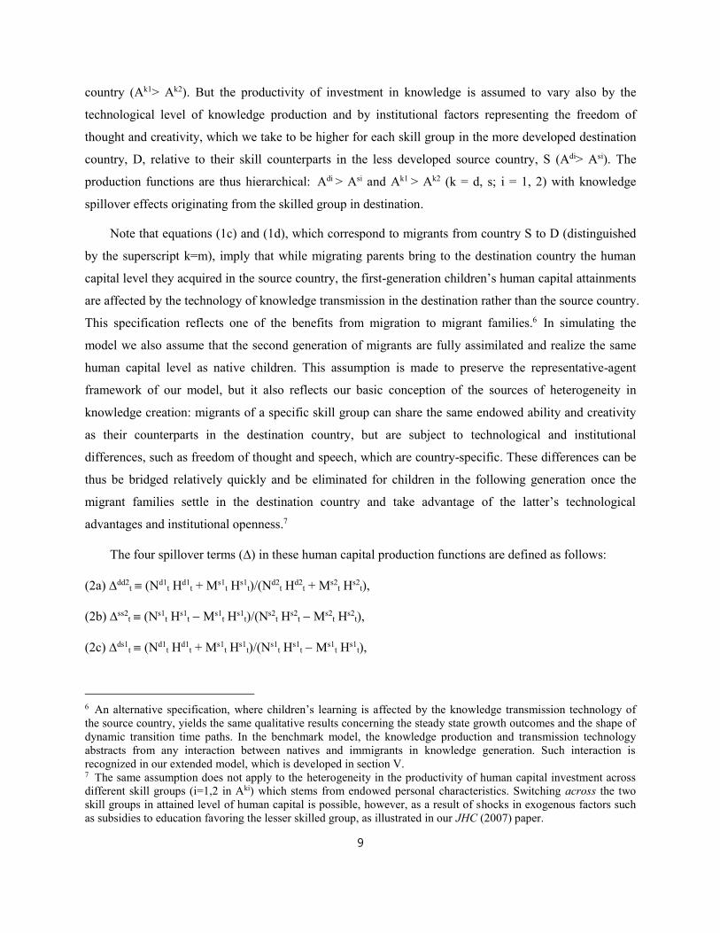
country (Ak1> Ak2). But the productivity of investment in knowledge is assumed to vary also by the

technological level of knowledge production and by institutional factors representing the freedom of

thought and creativity, which we take to be higher for each skill group in the more developed destination

country, D, relative to their skill counterparts in the less developed source country, S (Adi> Asi). The

production functions are thus hierarchical: Adi > Asi and Ak1 > Ak2 (k = d, s; i = 1, 2) with knowledge

spillover effects originating from the skilled group in destination.

Note that equations (1c) and (1d), which correspond to migrants from country S to D (distinguished

by the superscript k=m), imply that while migrating parents bring to the destination country the human

capital level they acquired in the source country, the first-generation children’s human capital attainments

are affected by the technology of knowledge transmission in the destination rather than the source country.

This specification reflects one of the benefits from migration to migrant families.6 In simulating the

model we also assume that the second generation of migrants are fully assimilated and realize the same

human capital level as native children. This assumption is made to preserve the representative-agent

framework of our model, but it also reflects our basic conception of the sources of heterogeneity in

knowledge creation: migrants of a specific skill group can share the same endowed ability and creativity

as their counterparts in the destination country, but are subject to technological and institutional

differences, such as freedom of thought and speech, which are country-specific. These differences can be

thus be bridged relatively quickly and be eliminated for children in the following generation once the

migrant families settle in the destination country and take advantage of the latter’s technological

advantages and institutional openness.7

The four spillover terms () in these human capital production functions are defined as follows:

(2a) dd2t (Nd1

t Hd1t + Ms1

t Hs1t)/(Nd2

t Hd2t + Ms2

t Hs2t),

(2b) ss2t (Ns1

t Hs1t Ms1

t Hs1t)/(Ns2

t Hs2t Ms2

t Hs2t),

(2c) ds1t (Nd1

t Hd1t + Ms1

t Hs1t)/(Ns1

t Hs1t Ms1

t Hs1t),

6 An alternative specification, where children’s learning is affected by the knowledge transmission technology of the source country, yields the same qualitative results concerning the steady state growth outcomes and the shape of dynamic transition time paths. In the benchmark model, the knowledge production and transmission technology abstracts from any interaction between natives and immigrants in knowledge generation. Such interaction is recognized in our extended model, which is developed in section V. 7 The same assumption does not apply to the heterogeneity in the productivity of human capital investment across different skill groups (i=1,2 in Aki) which stems from endowed personal characteristics. Switching across the two skill groups in attained level of human capital is possible, however, as a result of shocks in exogenous factors such as subsidies to education favoring the lesser skilled group, as illustrated in our JHC (2007) paper.

10

(2d) ds2t (Nd2

t Hd2t + Ms2

t Hs2t)/(Ns2

t Hs2t Ms2

t Hs2t),

where Nkit is the population size of natives with skill level i in country k, and Msi

t is the number of

migrants from country S to country D with skill level i. Equations (2a) and (2b) specify the within-

country spillover terms within D and S, respectively, and equations (2c) and (2d) specify the cross-

country spillover terms. The logic of these externality terms is the idea that knowledge spillover effects

flow from groups with higher human capital attainments to those with lower ones, and that the learning

benefits to the latter group are greater the larger the disparity between the human capital attainments and

population sizes of the two groups. Relative group size matter since a higher “teacher-student” ratio raises

the learning effectiveness for knowledge recipients.

C. Goods production

Consumption goods are produced by a production function that is subject to constant returns to scale

in the total flow of effective (human capital augmented) labor services, but is also subject to external

effects arising from the size of the labor force within sectors and the average level of workers’ human

capital. We assume that the labor market is competitive, generating full employment, and that the goods

produced in the “high-tech” and “low-tech” sectors are perfect substitutes in consumption. This

assumption sets the unit price of the good produced in S (normalized at 1) as the numeraire and eliminates

the need to consider any trade across both sectors and countries. The production function of the good

produced by skill group i in country D, is thus

(3) Qdit = di (Ndi

t Ldit Hdi

t + Msit Lmi

t Hsit) Ψdi,

where Ldit and Lmi

t stand for the total working hours of natives and immigrants in skill group i,

respectively. Equations (8) and (11) below indicate how these variables are determined, and ki is a

productivity parameter, specific to good i in country k. Ψdi denotes external effects as follows:

(3a) Ψdi = (NditHdi

t + MsitHsi

t)- [(NditHdi

t + MsitHsi

t)/(Ndit + Msi

t)],

= (Ndit + Msi

t)- [(NditHdi

t + MsitHsi

t)/(Ndit + Msi

t)]-, (>0, >0).

These external effects incorporate two components. The first represents a negative external effect arising

from the total number of workers (Ndit+Msi

t) due to some implicitly fixed factor of production such as a

fixed capital good, generating negative returns to the quantity of the labor force employed in sector i. The

second accounts for a positive external effect arising from the average worker’s level of human capital

due to interaction among workers in the work place (cf. Lucas, 1988). The latter represents an external

11

productive factor at time t (analogous to a physical capital input we abstract from for simplicity), which

evolves endogenously over time. The production function is thus:

(3b) Qdit = di (Ndi

t Ldit Hdi

t + Msit Lmi

t Hsit) (Ndi

t + Msit)-φ [(Ndi

tHdit + Msi

tHsit)/(Ndi

t + Msit)]-.

The constraints φ > 0, μ-φ > 0 assure the existence of an interior equilibrium solution for immigration.

A similar production function applies to country S, with the exception that those migrating to country

D are a drain on the labor force size in S. The production function of consumption goods by skill group i

in country S is

(4) Qsit = si (Nsi

t Msit) Lsi

t Hsit (Nsi

t Msit)-φ [(Nsi

t Hsit Msi

t Hsit)/(Nsi

t Msit)]-.

Since the labor market is competitive, the marginal product of effective labor per hour equals the

wage rate, or rental rate of a unit of effective labor, for workers in each sector of each country.

(5) dit = di (Ndi

t + Msit)- [(Ndi

tHdit + Msi

tHsit)/(Ndi

t + Msit)]-,

(6) sit = si (Nsi

t Msit)-φ [(Nsi

t Hsit Msi

t Hsit)/(Nsi

t Msit)]- = si (Nsi

t Msit)-φ(Hsi

t)-.

D. Preferences and motivating forces

As in our (2007) paper, we take parental altruism to be the underlying force motivating parental

demand for children. The utility function of a representative decision maker in country k (= d, s) with

skill level i (i = 1, 2) at period t is given by the additive function:

(7) U(Ckit, Wki

t) = [1/(1σ)][(Ckit)1-σ1] + [1/(1σ)][(Wki

t)1-σ1],

where δ denotes the inverse intertemporal discount factor (0<δ<1), σ denotes the inverse intertemporal

elasticity of substitution in consumption, and Ckit stands for real consumption spending of the native

parent in skill group i in country k, financed by her labor market earnings:

(8) Ckit = Lki

t kit Hki

t = (1 vk nkit ki hki

t nkit) ki

t Hkit.

In equation (8), nkit represents the number of children per parent and vk and ki are fixed unit costs,

measured as the time costs, or fractions of income, of nurturing and financing the child’s educational

investments, respectively. As in EK (2007a), the fertility unit costs vk are restricted to be equal for

different skill groups within countries to assure a balanced population growth path, but the educational

financing costs ki may vary across skill groups due to capital market imperfections. Equation (8) also

indicates that the total time endowment, normalized as 1, is spent on child rearing (vk nkit), child education

(ki hkit nki

t) and thus labor supply (Lkit) as well. The last term in equation (7),

12

(9) Wkit B (nki

t) (̃kit+1 Hki

t+1)α, with α =1 and >1,

represents the parental altruism function in an OLG context, borrowed from Ehrlich and Lui (1991),

which reflects the altruistic rewards parents obtain vicariously from the number of offspring and their

potential earnings. For analytical simplicity and numerical tractability, the future wage rate for children

(̃kit+1) is forecasted on the assumption that the population share of migrants and the human capital

growth rate in the children’s generation are the same as those in the parent’s generation. The restrictions

on the parameters α and are necessary for obtaining interior solutions for both hkit and nki

t. To ensure the

concavity of equation (7) we must further imposed the following restrictions: (1-)<1 (or, >0) and (1-

)<1.

For immigrants in country D with skill level i (i = 1, 2), the utility, consumption, and the altruism

functions are given by

(10) U(Cmit, Wmi

t) = [1/(1σ)][(Cmit)1-σ1] + [1/(1σ)][(Wmi

t)1-σ1],

(11) Cmit = Lmi

t dit Hsi

t = (1 vs nmit si hmi

t nmit i) di

t Hsit,

(12) Wmit B (nmi

t) (w̃kit+1 Hmi

t+1)α, with α =1 and >1,

where nmit represents the number of children per migrating parent in skill group i. By equation (11)

immigrants are assumed to possess the human capital attained by natives in country S, where they

received their education, but enjoy the wage rate obtained by natives of corresponding skills in country D.

They are also assumed to face the same cost of raising (vs) and educating a child (si) as their counterparts

in country S. Unlike the latter, however, migrants bear migration costs, measured as time costs or

fractions of full income due to moving and adjustment costs in D given by i.

The endogenous population formations of skill groups i in country D and S evolve dynamically as

functions of fertility and lagged population stocks as follows:

(13) Ndit+1 = ndi

t Ndit + nmi

t Msit,

(14) Nsit+1 = nsi

t (Nsit Msi

t).

E. Basic solutions

Representative members of each of the six population groups in the model select optimal fertility and

human capital investment in children which maximize the objective functions in equations (7) or (10),

subject to (8) and (9), or (11) and (12), taking {Hkit, ki

t, kit+1, Nki

t} as given.

1. Optimal fertility and human capital investments choices

13

The first-order optimality conditions involving fertility and human capital investment of natives in

skill group i (=1, 2) and country k (= d, s) are:

(for nkit >0) 0 = (Cki

t)-σ [ vk ki hkit] ki

t Hkit + δ (Wki

t)-σ B (nkit)-1 ki

t+1 Hkit+1,

(for hkit >0) 0 = (Cki

t)-σ [ ki nkit] ki

t Hkit + δ (Wki

t)-σ B (nkit) ki

t+1 (Hkit+1/ hki

t).

For migrants from S to D in skill group i, the conditions are

(for nmit >0) 0 = (Cmi

t)-σ [ vs si hmit] di

t Hsit + δ (Wmi

t)-σ B (nmit)-1 di

t+1 Hmit+1,

(for hmit >0) 0 = (Cmi

t)-σ [ si nmit] di

t Hsit + δ (Wmi

t)-σ B (nmit) di

t+1 (Hmit+1/ hmi

t).

Using these optimality conditions, we obtain an explicit solution for human capital investments:

(15) hkit = vk/ [ki(1)], (i = 1, 2; k = d, s)

(15a) hmit = vs/ [si(1)], (i = 1, 2)

By equations (15) and (15a) human capital investments hkit, can have interior and unique solutions, since

they apply under the general utility function given in equation (7). For fertility, nkit, we obtain just an

interior solution: The first order condition for nkit can be rearranged as

(16) (1vk nkit ki hki

t nkit)-σ = δ [B(nki

t)(kit+1/ki

t)(Aki/ki){vk/(1)}]-σ B(nkit)-1(ki

t+1/kit)(Aki/ki).

This equation implies that the solution for nkit depends on the ratio Aki/ki, or each group’s investment

efficiency, as in EK (2007a). If we specify the utility function in log form, however, we have an explicit

solution for fertility among native and immigrant skill group i=1,2 in country k = (d, s), or nkit and nmi

t

respectively:

(16a) nkit = (1)/ [vk (1+ )],

(16b) nmit = (1)[1 i] / [vs (1+ )].

2. Optimal migration

Agents with skill level i emigrate from country S to country D as long as the lifetime utility of

residing in D is higher than that in S. The equilibrium flow of migrants with skill level i at time t, Msit,

will be determined at the point where the utility level of the marginal migrant in country D and S are

equalized. The arbitrage condition governing the process is given by:

(17) (Cmit)1-σ + (Wmi

t)1-σ = (Csit)1-σ + (Wsi

t)1-σ (i = 1, 2).

14

Using the optimality conditions concerning human capital investment and fertility, we can transform

equation (17) to

(18) (1 vs nsit si hsi

t nsit)- [1 (1)(vs nsi

t + si hsit nsi

t)/] (sit)1-

= (1 vs nmit si hmi

t nmit i)- [(1 i) (1)(vs nmi

t + si hmit nmi

t)/] (dit)1- .

This condition implies that the flow of migrants is determined at the point where the wage rates, sit and

dit, become proportional at the equilibrium steady state. Alternatively, From (18), (di

t/sit)1- = [(1vs

nsitsi hsi

t nsit)/(1vs nmi

tsi hmit nmi

ti)]- [1 (1)(vs nsit + si hsi

t nsit)/] / [(1 i) (1)(vs nmi

t + si

hmit nmi

t)/], so the proportionality factor varies with the evolving values of fertility over the transitional

dynamic path, nkit (k=s,m), until a steady state is reached.

Equilibrium (18) presents a complex solution for the equilibrium migration flows since they are

intertwined with those of the model’s other control variables. More insight about the determinants of

equilibrium migration can be derived if we adopt a log utility function. In this case, optimal fertility, like

investment in human capital, has a unique solution which is constant over time in each country (see eq. 16

and 16a). The arbitrage condition in eq. (18) then becomes

(18a) sit (1 i) di

t = 0, or equivalently

f(Msit) = si (Nsi

t Msit)-φ(Hsi

t)- (1 i) di(Ndit + Msi

t)-[(NditHdi

t + MsitHsi

t)/(Ndit + Msi

t)]- = 0,

i.e., the equilibrium levels of migration flows of both skill levels are reached when the wage rate per unit

of human capital in the source country equals the corresponding wage rate in destination net of the

migration entry “tax” rate. Consequently, the following propositions hold under a log utility functional

specification:

Proposition 1. There is a positive and unique solution for the flows of all skill-specific workers choosing

to migrate from their source country to the destination country at any given time period (generation),

provided the following condition is met:

(19) (Ndit /Nsi

t) < (1 i) (Γdi/Γsi) (Hdit /Hsi

t)-.

Proof: In equilibrium f(Msi) = 0 by equation (18a). Equations (5) and (6) imply that sit/Msi

t > 0, and

dit/Msi

t < 0, and thus f(Msit)/Msi

t > 0. When Msit converges to its upper limit (= Nsi

t), we have f(.) →

. In contrast, when Msit converges to its lower limit (= 0), we have f(.) < 0 as long as equation (19) holds.

It follows that the function f(Msi) has a positive and unique solution at f(.) = 0.

15

Equation (19) has a simple interpretation: The LHS term represents the population stocks in

destination relative to source country and the RHS is controlled by the relative human capital stocks in

these countries. The condition implies that the prevailing human capital stock or labor productivity levels

in D relative to S should be high enough, and/or the prevailing population size in D relative to S should be

low enough, to attract a positive flow of immigrants, since these sets of factors contribute to a sufficiently

high wage premium in D relative to S.

Moreover, we can show that the stocks of skill-specific migrants are increasing functions of the

excess level of the skill-specific human capital in D over S:

Proposition 2. A rise in the human capital stocks of specific skill groups in the destination country (Hdit)

will increase the flow of migrants from the source country (Msi), provided that all other determinants of

migration in equation (18a) remain unchanged.

Proof: From Proposition 1, we know that function f(Msit) is rising in its argument. We can further show

that f(Msit)/Hdi

t = sit/Hdi

t (1 i) dit/Hdi

t =

(1 i) Γdi (-) (Ndit + Msi

t)- (NditHdi

t + MsitHsi

t)--1 Ndit < 0.

This condition implies that f(Msit) decreases when Hdi

t rises. Therefore, the optimal value of Msit in

equation (18a) where f(Msit) = 0 rises as Hdi

t increases.

While both propositions 1 and 2 are derived in the special case where utility is of the log form, we

conjecture that they apply more widely and are therefore testing them empirically (see section VII).

IV. Growth Equilibrium, Comparative Dynamics, and Transitional Paths in the Benchmark Model

A basic proposition following the mechanics of our open-economy model is that in a stable balanced

growth equilibrium, the growth rate of human capital, and thus full income in the global economy must

converge on the steady state growth rate of the skilled group in the destination country D, Ad1hd1 = (1+g)

in equation (20) below, since all spillover effects linking the 6 population groups comprising the global

economy originate from this group due to its highest technological prowess, or ability to generate new

human capital. We skip an elaborate proof of this proposition since it follows the logic of proposition 1 in

our earlier paper (EK, 2007). The necessary condition for attaining a balanced growth equilibrium path

can be derived from equation sets (1) and (2), and the solutions for optimal fertility and human capital

investment from the first-order optimality conditions in section III.5:

(20) dHkit+1/dHki

t = Ad1(hd1t)* = vd (Ad1/d1)/(1) = (1+g*) >1,

16

where (1+g*) = denotes the equilibrium growth rate of human capital formation. The attainment of a

growth equilibrium is thus conditional on the skilled group in destination having a sufficiently large level

of knowledge-production technology, Ad1, or a threshold level of parental investment in offspring’s

human capital, (hd1t)* > (1/Ad1) stemming from a sufficiently high unit cost of fertility, vd, a low unit cost

of education, d1, or a low preference for a large quantity of children, as indicated by equation (20).

Additional parameter restrictions need to be imposed, however, as sufficient conditions for obtaining

a balanced growth equilibrium path, apart from the concavity and independence of the decision makers’

utility functions. First, the ratios of human capital investment efficiencies must be equal across skill

groups within and across countries:

(20a) (Ad1/d1)/(Ad2/d2) = (As1/s1)/(As2/s2).

This assumption is needed to guarantee that the six family groups comprising the populations of receiving

and sending countries continue to have a stable representation in the distribution of human capital

formation within and across countries in any balanced global equilibrium steady state. A similar

restriction must also apply to the productivity parameters associated with the production functions of

consumption goods:

(20b) d1 / d2 = s1 / s2.

This condition assure that the relative wage rates, or rental values per unit of human capital are equalized

across the skill groups in each country, and thus allow for stable earnings distributions within and across

countries in any balanced equilibrium steady state. In contrast, we need to impose an asymmetry

condition on the unit cost-shares of rearing children in S vs. D:

(20c) vd > vs.

This restriction is necessary for obtaining a higher endogenous fertility in country S relative to D, which

is necessary for obtaining interior steady state equilibrium solutions for migration along with a balanced

population growth involving the source and destination countries (see also Appendix, part 1).

With these assumptions we derive a balanced growth equilibrium path with the following properties:

(i) fertility and population growth rates of both skill groups are constant and equal across both natives and

migrants in each country, i.e., Ms1t/Nd1

t = Ms2t/Nd2

t; and Ms1t/Ms2

t = Nd1t/Nd2

t; but the steady state fertility

rates remain higher in the source, relative to the destination country;

17

(ii) human-capital growth rates are equalized across skill groups and countries at the growth rate level of

the skilled group in the destination country, while population and fertility rates are equalized only across

skill groups within countries and among migrants;

(iii) wage and income disparity within and across countries are constant across the corresponding skill

groups;

(iv) a constant and persisting fraction of each skill group in S migrates to D. (See the simulation results in

Table 1).

As in EK (2007a), the model’s recursive dynamic system is too complex to be solved analytically via

any closed form solutions. We therefore resort to simulation analysis to derive numerical solutions for the

model’s key control and state variables in any global growth equilibrium steady state as well as over the

transitional dynamic paths over which the economy shifts from one steady state to another. We pursue our

simulations, however, under the general utility function as specified in equation (7), not under any special

functional form. The simulation methodology we use is explained in Appendix 1.

A. Comparative dynamics

Table 1 presents the comparative dynamics results of changes in the key parameters of our model

which are derived by simulating our benchmark model, using our general utility function as specified in

equation 7. The preference, discount, and spillover parameter values of the simulated model are taken

from EK (2007). The other parameters, including Aki, vk, and i are calibrated for the benchmark model so

that (i) the projected steady-state levels of fertility and per-capita full-income growth rates are on par with

those of the destination and source countries included in our empirical analysis in section VII, and (ii) the

steady-state fertility level of immigrants is intermediate between those of natives in S and natives in D.8

All external parameter values are listed in the legend to table 1. Assuming that one generation in our

model lasts 30 years, the projected long-term human capital growth rate in Table 1 is 2.34 percent per

annum (=2(1/30) – 1). The fertility levels in the benchmark case are 2.09, 3.22, and 2.52 for natives in D,

natives in S, and migrants, respectively (see case (i) of Table 1 for the benchmark case).

8 See Appendix. Part 1. The average annual growth rate of per capita GDP over the period (1975-2000) among the five destination countries in the sample used in our empirical investigation (Australia, Canada, France, UK and USA) is 2.25% and the one- generation (30 years) growth rate is thus 1.95 while our projected one-generation growth rate is 2 in table 1. The average total fertility rate (TFR) among the five countries in 1975 is 2.003 while the projected one is 2.0906. The average TFR among source countries with real per capita GDP (Penn World Table, 2012) higher than $5,000 is 3.19 while our projected fertility for source countries is 3.22. We exclude low-income source countries in this calibration since most may be in a stagnant equilibrium rather than in transition to growth equilibrium.

18

The central simulation of the numerical analysis, featured in case (ii) of Table 1, involves the “pull”

force of a skill-biased technological shock (SBTS) in human capital production which is assumed to

affect simultaneously only skilled workers in countries D and S.9 Both Ad1 and As1 are raised by 20

percent to simulate this case. The shock results in higher growth rates of both human capital and the wage

level, and thus in an even higher growth in full income, in D relative to S. The fertility rates in both D and

S also increase because of the resulting wealth effect10. While the wealth effect benefits skilled families

directly, it also affects unskilled families via the higher spillover effects reaching these families (see the

increase in dd2 and ss2 in Table 1). The ratio of skilled immigrants relative to skilled natives Ms1/Nd1 also

rises in D (see proposition 3 in section IV.2) while the ratio of skilled emigrants relative to natives in S,

Ms1/Ns1 falls.

In case (iii) we report the comparative dynamic results when we have a uniform technology shock

which affects all skill groups, implemented by uniformly raising all Aki by 20%. The resulting wealth

effect explains the increased fertility across all groups. The effect on the human capital growth rate in this

case is identical to that in the previous case, essentially because the growth rate in our model is dictated

by the skilled agents group. The change in the steady-state ratio of skilled migrants relative to skilled

natives is also identical to the case where the economy experiences a skill-biased technological innovation

which affects only the skill group in D. The changes in the immigration and emigration ratios are also

identical to the changes triggered by the SBTS case. However, the endogenous magnitudes of knowledge

spillovers (dd2 and ss2) are smaller because the uniform technology shock affects all groups.

Lowered immigration costs (τ) produce a positive income effects on all skill-groups in the economy,

which raises fertility (see case (iv) in Table 1, where τ is reduced by 20 percent). The human capital

growth rate is not affected, however, because optimal investment in human capital remains unaffected in

this case (see equation 15). The lower unit cost of migration naturally induces more emigration from S,

which raises the emigration ratios, Msit /Nsi

t, for both skill groups. However, the ratio of skilled migrant

9 The simultaneous adaptation of innovation in both countries, rather than in the more advanced country D where it typically occurs, is assumed to assure the existence of a globally balanced growth equilibrium steady state. We have also simulated a non-synchronized SBTS by which the skilled group in S receives the shock after a one period lag. These simulations yield the same qualitative effects as those reported in this section. Note that the comparative dynamics analysis of this section applies in principle to “push” factors originating in the source country as well. 10 Data assembled from all receiving countries indicate that the sharply declining trend in fertility in the major receiving countries following the end of the baby boom has changed course in all five countries since the mid-1970s. In the US, total fertility rate (TFR) hit the lowest level of 1.74 in 1976 and then rose to 2.00 in 2009. In France, TFR hit the lowest level of 1.836 in 1980 and then rose to 1.978 in 2009. In Australia and Canada the TFRs have generally leveled off and have been rising since the late 1990s. (See United Nations 2012, and World Bank 2014.)

19

relative to native populations, Ms1t /Nd1

t, falls, because the immigrants’ fertility, and therefore the native

population’s size going forward, rise even more. Note that this change in the immigration ratio represents

a long-run response; the immigration ratio may rise in the short run.

In case (v), we increase the unit cost of bearing and rearing children (vd) by 20% just in the

destination country. This lowers fertility but raises human capital investment per child due to a quantity-

quality tradeoff, as indicated by equation (15). The higher human capital investment rate raises the growth

rate of human capital formation in D (see eq. 20) and ultimately S because of the spillover effects running

from D to S. The resulting wealth effects bring about a rise, rather than a fall in fertility in the source

country because the latter does not experience a rise in the cost of fertility, unlike the destination country.

The full income in D therefore rises relative to that in S because of the higher relative human capital per

person in country D, which induces an increase in the ratio of immigrants in D and emigrants in S relative

to natives in both.

Case (vi) pertains to a simultaneous increase of the unit cost of fertility in both D and S. Not

surprisingly, in this case, both fertility rates are shown to fall and human capital investments to rise in S

as well, with the growth rate increasing as much as in case (v). But the ratios of skilled immigrants

relative to natives are here falling relative to case (v), but remaining the same as in the benchmark case.

B. Skill-biased technological shocks (STBS) and transitional dynamics

In this section we derive the transitional dynamic paths of the key endogenous variables of our model

following a skill-biased technological shock. We do it in order to derive the evolution paths of key control

and state variables over the transitional dynamic phase following the SBTS, such as the skill distribution

of migration flows, and income distribution measures (see figure 4 in subsection a) or the absolute level

of related variables, such as average human capital and wage levels (see figure 5 in subsection b).

We introduce the shock simultaneously in both country D and country S, by raising both Ad1 and As1

simultaneously, while leaving Ad2 and As2 intact. Specifically, we assume that the two economies are

initially at the equilibrium steady state we simulate in row (i) of Table 1. We then introduce an upward

shock raising Ad1 and As1 by 20 percent. The following is our theoretical prediction of the shock’s impact

on the skill composition of migration flows:

Proposition 3. A synchronized skill-biased technological shock that raises by equal proportions the

technology of knowledge creation by the skilled groups in both destination and source countries will

increase the skill composition of migrants along the transitional dynamic path leading to the balanced

growth steady state as well as the steady state ratio of skilled migrants to skilled natives in destination.

20

Proof: In any balanced growth-equilibrium steady state, the population growth rates are ultimately

equalized across skill groups in each country, or Ms1t/Nd1

t = Ms2t/Nd2

t, which in turn implies that relative

population ratios of skilled and unskilled groups are also ultimately equalized across native and

immigrant groups, or Ms1t/Ms2

t = Nd1t/Nd2

t.

These ratios deviate, however, over the transition to a new steady state following the SBTS, because of

the pattern of the direct- and between-skill-group spillover effects generated by the SBTS. Specifically,

the shocks in Ad1 and As1 raise directly the levels of Hd1 and Hs1, leaving unchanged Hd2 and Hs2. The

wealth effects generated thereby on the skilled groups in D and S will raise the optimal fertility of these

groups, nd1 and ns1, ahead of those of the unskilled groups, nd2 and ns2 since changes in the latter cannot

take place until the spillover effects of the increases in Hd1 and Hs1 take places. This will be repeated in

later generations as well since the spillover effects rise gradually over the transition to the new steady

state. Consequently the fertility rates of the unskilled workers will lag behind, but ultimately converge

with those of the skilled groups at the new steady state of growth. Skilled migrants will also have more

children than skilled natives in D because their fertility rates are higher than those of skilled natives. This

means that even if we have a constant skill composition of migrant flows, the equilibrium ratio of skilled

migrants relative to skilled natives in destination will increase in the steady state. But the lagged wealth

effect on fertility levels of the unskilled group in S would mean that the skill composition of migration

flows would be rising as well over the transition phase.

Proposition 4: A synchronized skill-biased technological shock that raises by equal proportions the

technology of knowledge creation by the skilled groups in both destination and source countries will

gradually increase the human capital level of skilled relative to unskilled groups in each country over the

transitional dynamic path leading to the balanced growth steady state as well as the in the steady state

itself.

Proof: The SBTS raises directly the technology of knowledge creation by skilled groups in both

destination and source countries, but has no such effect on the corresponding technology of unskilled

groups: the latter can increase only as a result of the spillover effects running from the skilled to the

unskilled in each country, kk2t (k=d,s). Consequently the SBTS first raises the ratio Hk1/Hk2 and the

effects of kk2t kick in gradually until Hk1/Hk2 converges on a higher steady state level.

a. Simulated transitional time paths of selected endogenous variables following the skill-biased

shock

Figure 4 illustrates the transitional dynamic paths of some key variables in Table 1 and related

variables following a skill-biased technological shock. The main findings are as follows:

21

(i) Consistent with proposition 3, the skill-biased shock in investment efficiency generates a gradually

rising path of the skill composition ratio in the migration flows, Ms1t/(Ms1

t+Ms2t), which converges on a

higher level in the steady state, as shown in panel a.

(ii) Likewise, the ratio of the skilled population relative to the total population in destination,

(Nd1t+Ms1

t)/(Nd1t+Ms1

t+Md2t+Ms2

t), gradually rises and reaches a higher steady state level following the

shock. Note that the simulated paths of these two ratios exhibit an immediate dip and a gradual

convergence to a new steady state (or growth equilibrium path).11

(iii) Consistent with proposition 4, panel c shows that the human capital level of the skilled relative to the

unskilled shows a gradually rising path and this ratio is the same over the whole transitional paths for

both destination and source country. This ratio rises in transition to a new steady state because the

spillover effect in human capital formation from the skilled to the unskilled in either country is steadily

rising over time after a shock. The full income ratio of the skilled to the unskilled, identical over the

transition for both countries, is shown in panel e to have a rising path as well.

(iv) A skilled bias technological shock raises the fertility rates of skilled natives and migrants in source

and destination countries due to the wealth effect coming from the shock in the same generation (see

panel d). However, the fertility rates of the less skilled agents will steadily rise and converge to those of

the skilled as the spillover effect gradually travels from the skilled to the less skilled.

(v) The shock also generates an upward sloping path of income inequality in both countries, as seen in

panel f. The skill composition and income inequality should then be positively correlated empirically as

long as the shock is skill-biased.

b. How the induced immigration following the SBTS affects the time paths of key endogenous

variables

Figure 4 illustrates how the skill-biased technological shock impacts the transitional time paths of

key control and state variables of the model in the destination country. It is interesting from a policy

perspective to decompose the total effect of the SBTS into the part that would be attributable to it if there

were no changes in the population share of skilled migrants in the destination country, and the part that

captures the contribution of the migration changes that are induced strictly by the SBTS. We attempt to do

that by simulating the dynamic paths under two scenarios: a. when the skill composition of migrant flows

11 This dip and other small oscillations that cannot be seen in charts portrayed in Figure 1 may be caused partly by our assumption concerning the way parents forecast children’s wages entering their altruism function in equation (9) (see Appendix 2).

22

and population shares are restricted to remain frozen at their initial steady state equilibrium values;12 b.

when no restrictions are imposed, as in the simulations of the benchmark model in Table 1.

The resulting transitional dynamic paths are shown in Figure 5. A solid line represents the time path

following the SBTS under the restricted scenario, while a hyphenated line in the same panel shows the

time path without any restriction on the equilibrium skill composition. Note that when the restricted path

is lower than the unrestricted path, this indicates that the variable’s level is higher in the unrestricted

scenario.

(i) Panel b shows that the skilled population ratio would be rising less sharply when the skill composition

is frozen, relative to the unrestricted case, and will actually start falling after a few generations following

the SBTS, partly as a result of the higher pace of growth of the entire population in the destination

country.

(ii) Panels c and d indicate that the average levels of both human capital and the wage rate (thus full

income per-capita) in the destination country are falling over the transition to a new steady state in the

restricted skill-composition scenario. This implies that in the unrestricted case, the endogenous rise in the

skill composition of migration contributes favorably to the average human capital and wage levels in D.

More interesting, panels g and h indicate that the increase in the wage level applies in the long term to

both unskilled and skilled workers in destination. In the unskilled workers’ case, panel h indicates that the

wage would be rising continuously in the unrestricted relative to the restricted scenario. In the skilled-

workers’ case, panel g indicates that the wage rate first falls following the SBTS, but after 10 generations

it starts rising continuously relative to its level in the restricted case even after 15 generations, which we

take to approximate convergence to a steady state based on the numerical results in Table 1.

Note that the rise in the wage level of both skill groups in the steady state comes from the SBTS-induced

rise in the skill composition of migrants relative to natives employed in consumer goods production (as

per proposition 3), which raises the average human capital level of the labor force employed in both

sectors of the economy (the Lucas-type externality). And as indicated by equations (5) and (6), the rise in

the average human capital of workers employed in each sector confers beneficial external effects on labor

productivity, which can offset the downward pressures on wages arising from higher quantities of labor

supply brought about by migration in the short run. The downward pressure on wages is higher in the hi-

tech sector relative to the low-tech sector due to the relative increase in the skilled migrants over the

12 Specifically we restrict the ratios Ms1/(Ms1+Ms2) and (Ms1/Nd1), both of which are required to pin down the share of skilled migrants flows, as well as their size relative to that of natives in the destination country’s population.

23

transition phase, which explains why their wages fall in the short run but not in the long-run, while the

wage rate of unskilled workers rises from the outset.13

(iii) Panel e shows that the fertility of skilled natives remains unaffected by the restrictions on skilled

migration. However, the fertility levels of unskilled natives would be falling under the restriction. The

average fertility level in the population would thus be higher when the skill composition is unrestricted.

(iv) Panel f indicates that unrestricted skilled migration reduces income inequality in destination relative

to the restricted migration case. The rise in the population share of skilled migrants under the unrestricted

immigration policy is found to lower the full income of skilled natives in the steady state following the

SBTS, but at the same time it confers a much larger increase in full income for the unskilled because of

the spillover effects conferred by skilled migrants. Migration thus lowers income inequality in the

benchmark model (see, however, section V).

V. Extended Model: Recognizing Complementarities between Natives and Immigrants in

Knowledge Production

Our benchmark model allows for interaction between native and migrant workers in goods

production through the external effect coming from the average level of human capital per workers of the

same skill. Such allowances have been generally recognized in other applications of endogenous growth

models (as in Lucas, 1988). In this section we extend the benchmark model by allowing for interaction

between natives and immigrants in the production of knowledge as well. The rationale for introducing this

extension is based on two considerations: 1. The production of human capital in equation set 1 allows for

the critical effects on the productivity of knowledge transmission and learning coming from parents and

from parental investments in their offspring, but not for direct inputs coming from the offspring

generation; 2. There is a large literature on diversity effects of immigration which indicates the existence

of complementarities between natives and migrants in production and innovation.

The literature is not uniform in support of positive diversity effects on productivity – differences in

language and culture may increase the costs of communication (Lazear 1999) – but diversity in

background and experience may enhance complementarities, especially across workers of the same skill

level who acquired their knowledge and skill in independent environments (the classical example being

the Manhattan project). Recent evidence (Alesina, Harnoss and Rappaport, 2015) indicates that birthplace

13 The population shares of both skilled and unskilled migrants relative to their native counterparts are equalized, however, in the steady state, as indicated by columns 9 and 10 of Table 1.

24

diversity has a net positive effect on productivity growth, especially for high skilled workers and in rich

countries. Our formal model can incorporate the possible effect of such diversity by allowing the

technological parameter controlling the productivity of knowledge generation and transmission in

equations (1a) – (1f ) to be an increasing and concave function of a simple measure of diversity involving

native and immigrant workers of the same skill level as follows:

(21) A̅ki (di) = Aki (1 + di) (k = d; i = 1, 2)

where di = Msi/(Ndi+Msi).

The diversity effect function di rises with Msi/Ndi ( 0), is equal to zero when Msi/Ndi = 0, and is

converging to 1 when Msi/Ndi goes to infinity. While the function is arbitrary in assuming that the

diversity effect is monotonic, it enables us to illustrate the potential effect of such diversity on the long-

run rate of productivity growth and the net benefits from immigration to both destination and source

countries.14

This is shown in the simulations reported in Table 2, where the comparative dynamics results of

Table 1 are now illustrated for the extended model using, for comparison, the same parameters as in Table

1. The assumed complementary relations between immigrants and natives leads to a higher growth rate of

human capital relative to our benchmark model, which raises fertility in both source and destination

countries relative to their levels in the benchmark model both at the initial equilibrium and following the

SBTS. Also, since the rate of investment in new knowledge is not affected, the productivity of investment

rises more in D relative to S, leading to a higher level of human capital formation, as well as higher wage

rate and full income in D relative to S. The latter effect implies that overall income inequality rises in D

relative to S as a result of the diversity effects of migration in our extended model. At the same time,

however, the net gain in destination rises absolutely, as well as relative to the source country, as we see in

section VI.

VI. Assessing the Long-Term Consequences of Migration on the Net Benefits to Natives

Our treatment of immigration as an endogenous variable in the context of an endogenous growth

model of the global economy offers new insights concerning the measurement of the net economic costs

and benefits associated with migration to natives in the destination and source countries what the

14 A monotonic impact of di could be justified in theory on the grounds that the population of country S in the model is a representative sample of diversity in countries of origin in the rest of the world. A larger d i would then always increase diversity. The equilibrium values of the endogenous diversity factors in our simulations are estimated to be 13.3% of the skilled group’s population. Curiously, a new release by the Center of Immigration Studies (see Zeigler and Camerota, 2015) puts the total number of foreign born population based on Center for Population Studies public use data for the second quarter of 2015 at 42.1 million or 13.3% of the population.

25

literature has often termed the “immigration surplus” (IS). The standard approach for measuring this

variable in a competitive economy, confined mostly to the destination country, is based on a static

framework in which the capital stock is a given constant, labor is homogeneous, and aggregate production

is subject to CRTS. The “surplus” is then necessarily positive in destination, provided that wages fall.

Specifically, if the derived-demand for labor is downward-sloping, the increased labor supply due to

migration causes an increase in total output but a fall in the wage bill of native workers. At the same time,

the positive returns to capital in destination more than outweigh the fall in the wage bill so the average

native wins. By the same analysis, the wage bill in the source country rises with emigration, which results

in a negative surplus in that country.

Variations in this “static approach” allowing for heterogeneous skills of natives and migrants and

adjustments in the economy’s capital stock affect the magnitude of the IS in the destination country, but

generally not its sign. Since migration is treated as an exogenous event, most measures of IS in the

standard approach evaluate the effect of immigration starting with an equilibrium state with zero

immigration. The IS thus measured is typically found to be less than 1% (see Borjas, 1995).

The IS measurement differs in our model for two reasons: it treats migration as an endogenous

variable and accounts for the way immigration interacts with the economies of both destination and

source countries when both move dynamically along balanced growth equilibrium paths. In this context,

as our analysis in item (ii) of section IV.2 part b has shown, the SBTS-induced rise in composition of

skilled migrants can generate a differential increase in both the average human capital and wage levels in

the economy over the transitional dynamic phase following the shock, as well as along the steady state

growth equilibrium path in the destination country. The existence of a positive immigration surplus in the

destination country no longer requires, therefore, a simultaneous reduction in the average wage rate and

even in the wage rate of skilled workers in the long-term.

We compute two measures of the long-term IS based on the two models simulated in sections IV.2

and V – the benchmark model in which there is no interaction between natives and immigrants in

knowledge production, and in the extended model which allows such interaction. To emphasize the

comparison with the traditional measures of IS we focus below on IS measurement in the destination

country.

Since immigration is an endogenous variable, we first compute it starting from an initial global

equilibrium in which total migration and its skill composition are positive, not zero. It is simulated as the

percentage difference in the full income per capita experienced by natives in D and S following a skill-

biased technological shock (SBTS) under 2 scenarios (similar to the method we use in part B of section

26

IV.2): a. when the skill composition of migrants is free to adjust following the SBTS; b. when the skill

composition is confined by an immigration policy restricting it to remain fixed at its initial level. The

difference (a-b) represents the net benefit from the unrestricted scenario. The IS thus measured is “partial”

in the sense that it captures the net benefits from free immigration in D just over the transitional dynamic

path following the SBTS. Note that since a new steady state can occur only if immigration is unrestricted

– under the restricted case the economy cannot attain a balanced growth equilibrium – the IS

measurement must be limited to a finite number of generations following the SBTS.

In our benchmark model, the resulting estimated values of IS in the destination country are

summarized in part A of Table 3 after 5, 10, and 15 generations following the technological shock. The

results are presented for alternative per-capita welfare indicators: human capital formation, full income,

consumption, and individual utility. The highest measure amounts to an increase of 1.48% in the natives’

full income per-capita (FIPC) after a period of 15 generations. This long period is selected because it gets

closer to the period in which the economy approaches a new steady state under the unrestricted

immigration case. In part A of Table 4 the same IS measure is illustrated in terms of a 0.003 (=4.142-

4.139) percentage points reduction in the average annual growth rate of FIPC following the SBTS in the

restricted, relative to the unrestricted, migration case.

Alternatively we provide quantitative measures of the “full” immigration surplus under two different

scenarios: a. when the share of skilled migrants among all migrants in D is freely determined at an initial

steady state of balanced growth; b. when either skilled or unskilled migration is disallowed. These

estimates are presented in parts B and C of Table 3. If skilled migration is disallowed altogether, the

difference in full income per-capita between the restricted and unrestricted cases is more pronounced than

in the benchmark case, amounting to IS = 79.8% of the FIPC after 15 generations or a persistent 0.376

percentage points (=4.142-3.766) gain in the latter’s annual growth rate over the 15-generations period

(see part B of Table 4). The opposite outcome occurs, however, when the destination country disallows

any unskilled migration. Here natives experience a gain of 33.0% in FIPC after 15 generations (IS = -

33.0%) or, alternatively, a gain in the FIPC annual growth rate of 0.068 percentage points (=4.142-4.200)

from the restricted relative to the unrestricted immigration case over a 15-generations period (see part C

of Tables 3 and 4).

Larger estimates of IS are computed in our extended model, which allows for positive

complementarities or “diversity effects” in knowledge production across natives and immigrants of the

same skill groups as modeled in section V. By this model, the IS in the case where all migration is

27

disallowed in the destination country amounts to a persistent gain of 0.593 percentage points (=4.803-

4.210) in the annual growth rate of full income per-capita after 15 generations (see part E of Table 4).

In the last columns of Tables 3 and 4 we report the IS estimates for the source country for each of the

scenarios we implemented in the destination country. In two cases – when the ratio of skilled migration is

frozen over the transition (parts A and D), the IS for the source country is of an opposite sign to that of

the destination country, i.e., natives in S gain whereas those in D lose from restrictions on the proportion

of skilled workers that can migrate to D. We may thus have a zero sum net gain globally in this case. It is

interesting, however, that in the extreme case where skilled migration is disallowed altogether, the natives

in both destination and source countries are net losers. Moreover, when all migration is disallowed in our

extended model where we allow for complementarity between natives and migrants in knowledge

creation (part E), there is a positive sum net gain for both destination and source countries, essentially

because diversity effects raise the growth rates in both countries.15

Clearly, the immigration surplus estimates in tables 3 and 4 are theoretical and subject to limiting

assumptions. The benefits from diversity may be more modest, but our model understates the net benefits

in the sending country by assuming that a SBTS, which generally occurs first in the more technologically

developed destination country, is simultaneously available to the sending country. Migrants may be an

important channel speeding up the pace of innovation adoption in the sending country. In the main, the

estimates in Tables 2 and 3 indicate that the long-term dynamic immigration surplus could far exceed its

static estimates both on the up side and the down side, which opens up opportunities for immigration

policies that could enhance the benefits of migration to both destination and source countries.

VII. Empirical Analysis

In this section, we test empirically two basic implications of the model: (i) higher levels of human

capital of specific skill groups in the destination country will increase the immigration flows of

corresponding skill groups from the source country, conditional on the other variables entering (18a) and

(19) remaining unchanged. These include the population levels and goods production technologies in D

and S, and mobility and adjustment costs for immigrants (Proposition 2); and (ii) a skill-biased

technological shock affecting both the destination and the source country will raise the ratio of skilled

migrants in the total migrant flow from source to destination countries (Proposition 3). To test both

15 We stress the cases where both countries benefit from unrestricted immigration, since the global growth “equilibrium” paths we derive in the model in these cases would also be stable equilibria in the sense that no country would have an incentive to resist immigration.

28

propositions we use a comprehensive panel data on immigration from about 200 countries into five

destination countries over the period 1975-2000. The underlying assumption behind the second test is that

this sample period captures the predictions of proposition 3 due to the information technology revolution

that has taken a significant step forward during the 1970s and has had a profound effect on the returns to

knowledge and skill. Both propositions are tested via fixed effects regression models specified below.

Note that the regression models we develop to test these propositions are estimated via an OLS estimation

method because the regression analysis does not test for any presumed direction of causality: all of the

variables entering equation (18a) are simultaneously determined in equilibrium.

1. Variables used

A. Stock levels of skilled migrant populations (SM). Data on international migration are available from the

World Bank’s Panel Data on International Migration 1975-2000 (Schiff and Sjoblom, 2011). These data

contain information about the total number of migrants by educational attainment from 190 source

countries to 6 key destination countries in the OECD: Australia, Canada, France, Germany the UK and

the US. We do not utilize data for Germany in our regression analysis because of the East-West division

in that country over the sample period. The World Bank data are estimated to represent approximately 77

percent of the world’s migrant population. Both the total number of migrants [TOM] and the number of

skilled migrants [SM] are defined as stock variables. For example, [SM] is defined as the number of

immigrants with at least some college education, i.e., 13+ years of schooling residing in a destination

country by the country of birth.

B. Other correlates: Data on real per capita GDP [GDPc] in source and destination countries are taken

from the Penn World Table sample (Heston et al., 2012). These variables are used as proxies for missing

data on the average human capital (education) levels of skilled natives and migrants in destination and

source countries. We also use as correlates other variables that have been used in the literature to account

for mobility and adjustment costs to migrants. Data on such proxies as distance between countries [DIST],

language similarity [COMLANG], colonial experience [COLONY] and contiguity between the

destination and the source countries [CONTIG] are collected from the GEODist dataset (Mayer et al.,

2011). We use fixed-effects regression models to account for differences in production technologies in

destination and source countries. Summary statistics are given in Table 5.

1. Model specification

a. Testing proposition 2

The regression specification we develop to test proposition 2 using our panel data links the

equilibrium flow of skilled immigrants over the sample period 1975-2000 with the equilibrium values of

29

its associated correlates in equation (18a). Since our data include stock measures of the migrant

populations in receiving countries, rather than flow measures, we first need to convert the stock measures

into a flow-equivalent form. The regression model thus involves two steps:

In the first step we adopt a conversion method used in Ehrlich and Kim (2007) to specify migration

stock values as functions of past migration flows using a growth regression format. In this format the

observed stock of the skilled migrant populations (SMsdt) in the destination country at any year t is

expressed as a function of its initial value in year 0 and the average growth rate of the net migration flows

that accumulated over the period 0-t, g(t), as follows:

(22) SMsdt = (SMsd0) exp[g(t)t] exp(sdt),

where subscripts s, d, and t denote source country, destination country, and year, respectively, and sdt

stands for a random error.

The average growth rate thus estimated accounts for the average annual migration flow that

accumulated over the preceding t periods. Since the WB sample does not report the average migration

flows through t, g(t), we estimate the latter as a function of the determinants of the equilibrium migration

flows as specified in proposition 2, including proxies for the migration “tax” variable, the average human

capital levels of skilled migrants, and the goods-production technology parameters in destination and

source countries. Empirically we define skilled migrants in the WB panel as those with at least college

education. But there are no international panel data on the human capital or per-capita real income levels

of this group in the destination and source countries. We have used instead real per capita GDP levels in

destination and source countries as proxies. The function g(t) is thus specified to take the following form:

(23) g(t) = 1 + 2lnGDPcdt + 3lnGDPcst + 4Xsdt ,

where Xsdt includes the other measurable determinants of migration stocks in equation (18a), which

approximate our theoretical “migration cost” variable.

Taking a log transformation of equation (22) and combining it with equation (23) we link the stock

of skilled migrants from S to D at time t to its flow determinants through their interaction with the time

period elapsing from the stock’s initial value at t=0 as follows:

(24) lnSMsdt = 0 + 1 t + 2 tlnGDPcdt + 3 tlnGDPcst + 4 tXsdt + 5 lnTOMsdt +ust +dt +sdt .

In equation (24) the interaction terms of the time trend variable with any regressor estimates the impact of

that variable on the average growth rate of skilled migration flows through year t, and ust and dt account

for country-specific fixed effects in the source and destination countries. We include as an additional

30

regressor the total number of immigrants (TOM) in order to control for the varying dimensions of the

migration populations in different countries. Proposition 2 can be tested by its consistency with the

qualitative values of the estimated regression coefficients of equation (24).

b. Testing proposition 3

We employ a different econometric specification to test proposition 3 by estimating the shape of the

transitional dynamic path of skilled migrants following the SBTM, which is assumed to take place during

our sample period. In this analysis we convert the stock of skilled migrants (SM) to a concurrent flow

term by taking the first difference of SM over two consecutive periods:

(25) SMsdt SMsdt+1 SMsdt.

For the resulting flow variable SM serving as a dependent variable we use a standard linear model with

country-specific fixed effects:

(26) lnSMsdt = 0 + 1lnTOMsdt + 2T + 3GDPcdt + 4GDPcdt2 + 5GDPcdt

3

+ 6lnGDPcst + 7Xsdt + ust + dt + sdt.

In equation (26) we enter the proxies for the relative human capital levels in the destination countries –

GDP per capita – in cubic form to estimate the trend of the skilled migration flows as predicted by

proposition 3 and solved numerically in section IV.2. We also control for GDP per-capita in the source

country using a linear as well cubic transformations, which yield similar results. To convert the dependent

variable measuring the flow of skilled migration into its share in concurrent total flow of migrants, as

defined in proposition 3, we enter as an additional variable the total number of immigrants in log form

(TOM). We also add correlates comprising the X vector in equation (26), including language similarity,

past colonial status, distance, and contiguity.

Note that the de-trended first differences are expected to pick up high frequency variations and this

specification is therefore preferred for testing the model’s implications over the transitional dynamic

phase.

2. Results

The results of the regression specification in equation (24) are reported in Table 6. We find the

following:

(i) The coefficient for the time interaction term with lnGDPcdt indicates that higher per capita GDP in

destination, as a proxy for the human capital level of the skilled, is associated with higher skilled

immigration flows. This finding is consistent with the prediction in Proposition 2.

31

(ii) We also find that lower per capita GDP in S – a proxy for lower level of human capital of skilled

workers in S – is associated with more skilled immigrants, as implied in Proposition 2.

(iii) The binary variable indicating whether the source country and the destination country share a

common language (COMLANG) is shown to have a negative effect on the flow of skilled immigrants. In

a separate regression we conducted, where we use the total flow of immigrants as a dependent variable

instead of skilled migrants (not reported here), we find that COMLANG has a positive sign. This

indicates that the language barrier may work as a migration cost factor only for unskilled workers. The

binary variable (COLONY), indicating whether the source country and the destination country have ever

had a colonial link would be expected to reduce the adjustment costs to skilled migrants, as shown.

(iv) Higher migration cost due to longer distance between the destination and the source country (DIST)

reduces immigration by skilled migrants as it increases the mobility costs to migrants.

(v) We find that when the destination country is contiguous to the source country, skilled migration falls

while unskilled migration rises (the regression with total immigrants as the dependent variable is not

reported here). The reason may be that since distance is already controlled for in the regression, contiguity

may pick up the influence of area-specific employment opportunities which are more likely to involve

workers with low skills from contiguous areas, whereas the demand for skilled workers is wider in scope.

Table 7 reports the results of estimating equations (26) as a test of Proposition 3. Regression model 1

is a baseline model while model 2 includes a few extra regressors. The findings are:

(i) The per capita GDP levels in linear, quadratic and cubic forms are shown to be significant. The

estimated regression line based on the results from Table 7 is shown in Figure 6. The graph indicates a

steady increase in the skill composition ratio over the development process, as predicted in Proposition 3.

It virtually duplicates the shape of the transition dynamic path of the skill composition of migrant flows as

simulated in Figure 1, panel a.

(ii) Model 2 in table 7 confirms the negative association between immigration flows and DISTANCE as a

factor accounting for the mobility costs of immigration that inhibit skilled migration between S and D

along the transitional path linking the original growth equilibrium steady state with a more highly

developed steady state in D, while contiguous destination countries attract less skilled immigrants.

VIII. Concluding Remarks

The distinct feature of the this paper relative to extant literature is the treatment of migration flows

and their skill composition as endogenous variables within a balanced-growth equilibrium setting that

32

accounts for the interaction between receiving and sending countries. The model extends the framework

we used in our JHC paper (EK, 2007a) to analyze the joint determination of income growth and

distribution in a closed economy into an open economy setting with free international labor mobility, in

which migration flows remain positive even in a steady state of balanced growth.

To achieve the complex task, we resort to a number of simplifying assumptions. The only

reproducible asset in the economy is human capital. We abstract from the separate role of physical capital

and trade in goods by allowing for two segmented goods-producing sectors in destination and source

countries that employ exclusively one of the two skill groups of natives and immigrants and produce

high-tech or low-tech goods that are perfect substitutes in consumption. To obtain a balanced-growth

equilibrium and interior solutions we also need to restrict the relative magnitudes of some structural

parameters to be identical either across the two skill groups within an economy or across the two

economies. This rigid structure enables us, however, to focus on the role of human capital not just in

producing new knowledge, but also in generating external spillover effects that link together all the six

groups of households and workers comprising the global economy. In this context we offer two versions

of our general model: a benchmark model that abstracts from any complementarities in knowledge

production between natives and immigrants; and b. an extended model in which such complementarities

are recognized.

The main new insights offered by both versions of the model concern the observed rising trends in

both the skill composition of migration flows and in population share of skilled migrants relative to that

of natives in major immigration-receiving countries over at least four decades when “skill” is indexed as

the population share of adults with 13+ years of education. Our model forecasts both trends to be an

outcome of demand “pull” factors resulting from a skill-biased technological shock (SBTS), such as the

one generated by the IT revolution, which became widely spread over the 1970s, coinciding with a

significant and continuing surge in migration in the US after 7 decades of decline.

Such immigration patterns do not apply as a general rule to other historical migration trends or waves

– a current example being the immigration wave from the Middle East and Africa to EU countries, which

appears to be the result of “push factors”. The comparative dynamic predictions of our model can project

alternative patterns of migration trends or waves that result from shocks in exogenous parameters that

capture e.g., catastrophic events in sending countries. The more general insight offered by our model is

that significant changes in the migration flows and stocks can be more fully understood if treated as

endogenous outcomes of exogenous structural parameter shifts, including changes in government

immigration policies, but at the same time reflecting behavioral responses by potential migrants in source

33

countries, as well as equilibrating market forces that include interaction effects between destination and

source countries.

In this context our model offers new insights concerning the long-term consequences of endogenous

migration flows on major macroeconomic variables including the level and rate of growth of human

capital formation, wage rates of workers with specific skills, and income growth and distribution in both

receiving and sending countries, as summarized in sections IV and V. Our numerical analysis indicates

that an SBTS-induced rise in the skill composition of migration flows and their relative population shares

is expected to enhance the level (as in the benchmark model) or both the level and long-term rate of

growth (as in the extended model) of human capital formation and full-income per-capita in destination

countries, but at the same time exert an ameliorating effect on the growth in income inequality resulting

from the SBTS itself.

Whether the same effects apply in sending countries, however, is ambiguous. While long-term rates

of growth are expected to equalize along the balanced growth equilibrium paths by both versions of the

model, the impact on the source country’s level of human capital formation and income growth and

distribution goes in an opposite direction in the benchmark version of our model, but in the same

direction in our extended model which allows for complementarities in knowledge production across

immigrants and natives in destination.

A similar ambiguity applies to the long-term impact of SBTS-induced rise in the skilled migration

flows and relative population shares on the net benefits to natives in destination and source countries.

Destination countries may always gain from such migration trends. Moreover, estimates of the

“immigration surplus” to natives in destination are found to be significantly larger than those projected in

static models, as summarized in section VI. But the consequences for receiving and sending countries go

in opposite directions if measured over the transitional dynamic path of the economy following the skill-

biased shock or by estimating what natives in each country stand to lose if skilled or unskilled migration

is disallowed. Both countries stand to gain from unrestricted migration however in two major scenarios:

when there are no restrictions (in the benchmark case) and when all migration is unrestricted (in the

extended case allowing for diversity effects in knowledge production. Another insight that is supported by

both versions of our model is that the long run positive immigration surplus produced by a skill-biased

technological change comes about jointly with a rise in the average wage in the economy, even for skilled

workers in the ultimate steady state. That is, the net benefits for natives in this case do not require a fall in

the wage bill of natives in absolute terms. The immigration surplus is especially large for unskilled

34

natives in destination since the SBTS generates spillover effects in knowledge acquisition that are

especially favorable for his group.

Appendix A

Methodology of simulations

We calibrate the model by selecting the values of key parameters of the model to approximate the

average levels of fertility and per-capita income growth in the set of major destination countries as well as

the average fertility level of middle-income source countries, as reported in the international panel of the

World Bank’s data we explore in the regression analysis of section VII, subject to the sufficient

parametric conditions for global equilibrium we need to impose in order to obtain balanced growth

equilibrium paths for D and S. The parametric restriction that unit fertility costs be higher in destination

relative to source country in equation (20c) is also justified by the higher labor market opportunities of

females in the more developed destination, relative to source countries. We further restrict the fertility

rate of immigrants to be of intermediate level between source and destination countries because we expect

the opportunity costs of migration to exert an adverse income effect on migrant families’ desired fertility.

The numerical solutions for the steady state values of the key control and state variables of our

model in this case are derived in two steps. In the first step, we solve the three first-order conditions

(FOCs) for nd1t, ns1

t and nm1t in section III.5 and the arbitrage condition for Ms1

t (equation 17) to derive the

steady state values of nd1t, ns1

t, nm1t, and Ms1

t/Ns1t.16 The values obtained from the first step are then

plugged in the next step where we solve for a related set of four equations (three first-order conditions for

nd2t, ns2

t and nm2t, and the arbitrage condition for Ms2

t) to derive the steady state values of nd2t, ns2

t, nm2t,

and Ms2t/Ns2

t. These two steps can be performed sequentially because the spillover effects are assumed to

flow in just one direction: from the skilled to unskilled groups in our model.

We have explicit solutions for optimal investments in human capital from equations (15) and (15a).

The steady state values of all the other endogenous ratios in the model, such as Nsit/Ndi

t, and dit/si

t, can

be derived from equations 1, 2, 5, 6, 13 and 14 as well as the imposed condition that the stock levels of

population and human capital are growing at the same rate in both countries.

16 We do so by dividing both sides of the FOCs by (ki

t Hkit)1- and imposing the growth-equilibrium steady state

conditions; e.g., (kit+1/ki

t) = (Nkit+1/Nki

t)- (Hkit+1/Hki

t)- in equation (5).

35

The comparative dynamics results reported in Table 1 are derived by exogenously changing the

benchmark levels of the key parameters that can trigger a skilled-bias technological advancement and thus

generate a shift in the economy’s initial BGP to a higher level.

The simulations of transitional dynamics (shown in Figures 1 and 2) are conducted by tracing the

transitional evolution paths of our key control variables, starting from their values at the initial growth

equilibrium steady state and ending at the new growth equilibrium steady state. The major shock we

introduce is a skill-biased technological innovation favoring the skilled groups in both D and S, by

simultaneously raising Ad1 and As1 by the same proportion, with Ad2 and As2 held constant. The initial

values of the state variables, Hkit and Nki

t, are arbitrarily imposed without loss of generality, which can

then give rise to dynamic paths of our basic state variables as well as derivative variables like the skill

composition ratio of migrants and the Gini coefficient. In deriving the paths, we also use the three first-

order conditions and the arbitrage condition as we do in the derivation of the steady state values, but

without imposing any conditions that hold just in a steady state.

Explaining the “oscillations” in Figure 1 panels a and b of section IV.2

The assumption on parental forecast of children’s wage invoked in our numerical analysis results in

some oscillations in the transitional dynamic paths of the skill composition of migration flows and stocks

along the transitional dynamic paths of these variables. In Figure 1, panels a. and b., for example, the

simulated time paths of the skill composition of migration flows, as well as the ratios of the skilled

population relative to the total population experience a dip following a skill-biased technological shock.

Such dips can be rationalized as follows: Skilled parents aiming to migrate to D following a skill-biased

technological shock forecast the differential wage level between the destination and source countries to

remain the same as before the shock in D and S. This makes migration less gainful initially because

potential migrants face significant mobility and adjustment costs due to loss of earnings in S. However, as

the expanded difference between the wage levels in D and S is realized, the migrants’ expectations adapt

and the ratios of [Ms1/(Ms1+Ms2)] and (Ms1/Ns1) start moving upward. Oscillations may persist in future

periods (a la the Cobweb model) but they become much smaller since the ultimate wage differential in the

steady expands in the direction of D due to the higher endogenous growth of human capital in D relative to

S over the dynamic transition phase. The upward trend in migration flows to D will thus persist until the

actual growth rates in both D and S equalize as the economies converge on their new steady states. The

assumed forecast by parents may then overstate the actual difference before D and S reach their steady

states.

36

References

Alesina, Alberto, Johann Harnoss, and Hillel Rapoport. 2013 (updated 2015). “Birthplace Diversity and Economic Prosperity. NBER Working Paper No. 18699. I guess you can change this in the text as well with the year stated as 2015, if proper, since it was updated in October 2015.

Barro, Robert J., and Jong Wha Lee. "A new data set of educational attainment in the world, 1950–2010." Journal of development economics 104 (2013): 184-198.

Becker, Gary, Kevin Murphy, and Robert Tamura. "Economic growth, human capital and population growth." Journal of Political Economy 98, no. 5 (1990): S12-S137.

Borjas, George J. Self-selection and the earnings of immigrants. No. w2248. National Bureau of Economic Research, 1987.

Borjas, George J. "The Economic Benefits from Immigration." Journal of Economic Perspectives 9, no. 2 (1995): 3-22.

Brücker, Herbert, and Cécily Defoort. "Inequality and the self-selection of international migrants: theory and new evidence." International Journal of Manpower 30, no. 7 (2009): 742-764.

Brücker, H., Stella Capuano, and Abdeslam Marfouk. "Education, gender and international migration: insights from a panel-dataset 1980-2010." Mimeo, 2013.

Clark, Ximena, Timothy J. Hatton, and Jeffrey G. Williamson. "Explaining US immigration, 1971-1998." The Review of Economics and Statistics 89, no. 2 (2007): 359-373.

Drinkwater, Stephen, Paul Levine, Emanuela Lotti, and Joseph Pearlman. "The immigration surplus revisited in a general equilibrium model with endogenous growth*." Journal of Regional Science 47, no. 3 (2007): 569-601.

Ehrlich, Isaac, and Francis T. Lui. "Intergenerational trade, longevity, and economic growth." Journal of Political Economy (1991): 1029-1059.

Ehrlich, Isaac, and Jinyoung Kim. "Social security and demographic trends: Theory and evidence from the international experience." Review of Economic Dynamics 10, no. 1 (2007): 55-77.

Ehrlich, Isaac and Jinyoung Kim. "The Evolution of Income and Fertility Inequalities over the Course of Economic Development: A Human Capital Perspective." Journal of Human Capital, vol. 1 (Winter, 2007) 137-74.

Galor, Oded, and Omer Moav. "From physical to human capital accumulation: Inequality and the process of development." The Review of Economic Studies71, no. 4 (2004): 1001-1026.

Heston, Alan, Robert Summers and Bettina Aten, Penn World Table Version 7.1 Center for International Comparisons of Production, Income and Prices at the University of Pennsylvania, November 2012.

Idu, Roxana. "The endogenous skill composition of migration and migrant inequality over the course of economic development." PhD diss., State University Of New York At Buffalo, 2012.

Kahanec, Martin, and Klaus F. Zimmermann. "Migration, the quality of the labour force and economic inequality." (2008).

Lazear, E. P. (1999b), "Culture and Language." Journal of Political Economy, 107(6): 95-126.

37

Lucas, Robert E. "On the mechanics of economic development." Journal of monetary economics 22, no. 1 (1988): 3-42.

Lundborg, Per, and Paul S. Segerstrom. "International migration and growth in developed countries: a theoretical analysis." Economica 67, no. 268 (2000): 579-604.

Lundborg, Per, and Paul S. Segerstrom. "The growth and welfare effects of international mass migration." Journal of International Economics 56, no. 1 (2002): 177-204.

Mayer, T. & S. Zignago. “Notes on CEPII’s distances measures: the GeoDist Database” CEPII (French Research Center in International Economics) Working Paper 2011-25, 2011.

Romer, Paul M. "Endogenous Technological Change." Journal of Political Economy 98, no. 5 pt 2 (1990).

Schiff, Maurice and Sjoblom, Mirja Channa "World - Panel Data on International Migration 1975-2000", The World Bank, 2011.

Smith, James P. “The Human Capital (Schooling) of Immigrant’s in America”, Handbook of International Migration, 1A, Chapter: 4, (2014)

Stokey, Nancy L. "Learning by doing and the introduction of new goods." The Journal of Political Economy (1988): 701-717.

United Nations, Department of Economic and Social Affairs, Population Division. 2014. The 2012 Revision of World Population Prospects. World Bank. 2015. The World Development Indicators. Zak, Paul J., Yi Feng, and Jacek Kugler. "Immigration, fertility, and growth."Journal of Economic Dynamics and Control 26, no. 4 (2002): 547-576.

Zeigler Karen and Steven A. Camarota, Immigrant Population Hits Record 42.1 Million in Second Quarter of 2015, Center for Immigration Studies, August 2015.

38

Table 1: Simulating Comparative Dynamic Effects of Parameter Changes - Benchmark Model

(1) (2) (3) (4) (5) (6) (7) (8) (9) (10) (11) (12) (13) (14)

nd1

= nd2 ns1

= ns2 nm1

= nm2 hd1

hd2

hs1

= hm1 hs2

=hm2 Growth Rate*

Ms1/ Nd1

= Ms2/ Nd2

Ms1/ Ns1

= Ms2/ Ns2

dd2 = ss2

ds1 = ds2

Hd1/ Hs1

= Hd2/ Hs2

d1/ s1

= d2/ s2

(i) Initial steady state 2.0906 3.2207 2.5157 0.2 0.2 0.1333 0.1333 2 0.1803 0.2101 5.6569 4.8140 3.0820 1.5728 (ii) Ad1 =12, As1 =9.6 2.1198 3.2642 2.5508 0.2 0.2 0.1333 0.1333 2.4 0.1807 0.2094 8.9234 4.8140 3.1025 1.5785 (iii) Ad1 =12, As1 =9.6,

Ad2 =6, As2 =4.8 2.1198 3.2642 2.5508 0.2 0.2 0.1333 0.1333 2.4 0.1807 0.2094 5.6569 4.8140 3.1025 1.5785

(iv) 1 = 2 = 0.16 2.0907 3.2208 2.6436 0.2 0.2 0.1333 0.1333 2 0.1664 0.2143 5.6569 4.8140 2.7713 1.4874 (v) vd =.072 1.7462 3.2659 2.5287 0.24 0.24 0.1333 0.1333 2.4 0.2282 0.2886 5.6569 7.5938 4.0429 1.7247 (vi) vd =.072, vs =.048 1.7470 2.6912 2.1023 0.24 0.24 0.16 0.16 2.4 0.1804 0.2100 5.6569 4.8140 3.0861 1.5739

Note: Parameters for the benchmark case: Ad1 =10, As1 =8, Ad2 =5, As2 = 4, 1 = 0.2, 2 = 0.2, vd = 0.06, vs = 0.04, d1 = 1, d2 = 1, s1 = 1, s21 = 1, = 0.9, = 0.7, = 1.3, 1 = 0.4, 2 =0.4, = 0.1, = 0.6, B = 1, d1 = 1, s1 = 1, d2 = 1, s2 = 1. * The projected steady state growth rate is for human capital formation over 1 generation. Comparative dynamics in the GE steady state are simulated by decreasing 1, 2, or increasing Ad1, As1, Ad2, As2, vd, vs by 20 percent, holding other parameters constant at the benchmark values.

39

Table 2: Simulating Comparative Dynamic Effects of Parameter Changes – Extended Model

Allowing for Diversity Effects in Knowledge Formation

(1) (2) (3) (4) (5) (6) (7) (8) (9) (10) (11) (12) (13) (14)

nd1

= nd2 ns1

= ns2 nm1

= nm2 hd1

hd2

hs1

= hm1 hs2

=hm2 Growth Rate*

Ms1/ Nd1

= Ms2/ Nd2

Ms1/ Ns1

= Ms2/ Ns2

dd2 = ss2

ds1 = ds2

Hd1/ Hs1

= Hd2/ Hs2

d1/ s1

= d2/ s2

(i) Initial steady state 2.1109 3.2510 2.5401 0.2 0.2 0.1333 0.1333 2.2664 0.1537 0.2306 5.6569 6.5806 3.2198 1.5768 (ii) Ad1 =12, As1 =9.6 2.1401 3.2945 2.5752 0.2 0.2 0.1333 0.1333 2.7203 0.1540 0.2300 8.9234 6.5846 3.2413 1.5825 (iii) Ad1 =12, As1 =9.6,

Ad2 =6, As2 =4.8 2.1401 3.2945 2.5752 0.2 0.2 0.1333 0.1333 2.7203 0.1540 0.2300 5.6569 6.5846 3.2413 1.5825

(iv) 1 = 2 = 0.16 2.1098 3.2493 2.6677 0.2 0.2 0.1333 0.1333 2.2501 0.1429 0.2334 5.6569 6.4631 2.8921 1.4909 (v) vd =.072 1.7663 3.3017 2.5575 0.24 0.24 0.1333 0.1333 2.7811 0.1887 0.3188 5.6569 10.976 4.2373 1.7319 (vi) vd =.072, vs =.048 1.7640 2.7164 2.1226 0.24 0.24 0.16 0.16 2.7198 0.1537 0.2305 5.6569 6.5814 3.2241 1.5779

Note: Parameters for the benchmark case: Ad1 =10, As1 =8, Ad2 =5, As2 = 4, 1 = 0.2, 2 = 0.2, vd = 0.06, vs = 0.04, d1 = 1, d2 = 1, s1 = 1, s21 = 1, = 0.9, = 0.7, = 1.3, 1 = 0.4, 2 =0.4, = 0.1, = 0.6, B = 1, d1 = 1, s1 = 1, d2 = 1, s2 = 1. * The projected steady state growth rate is for human capital formation over 1 generation. Comparative dynamics in the GE steady state are simulated by decreasing 1, 2, or increasing Ad1, As1, Ad2, As2, vd, vs by 20 percent, holding other parameters constant at the diversity model’s benchmark values.

40

Table 3: Immigration Surplus: Percentage Change in Welfare Measures’ Level When Migration is Restricted (Positive Values = Loss from Restriction= IS Gain)

Destination Source 5th generation

after a SBTS 10th generation after a SBTS

15th generation after a SBTS

15th generation after a SBTS

A. Skill composition held constant

Human capital 0.63 1.10 1.53 -26.4 Full income 0.67 1.15 1.48 -23.7 Consumption 0.67 1.15 1.47 -23.8 Utility 0.18 0.32 0.43 -7.36 B. skilled migration disllowed

Human capital 33.1 62.6 81.4 98.7 Full income 28.9 59.9 79.8 99.9 Consumption 42.2 67.5 83.6 99.9 Utility 10.0 23.1 35.2 49.8 C. Unskilled migration disallowed

Human capital -12.8 -21.2 -28.7 98.4 Full income -14.6 -24.1 -33.0 98.5 Consumption -13.4 -22.6 -31.2 98.5 Utility -3.65 -5.68 -7.30 60.9 D. Diversity: Skill composition held constant

Human capital 0.86 1.43 2.05 -14.5 Full income 1.07 1.77 2.40 -2.44 Consumption 1.07 1.77 2.38 -2.75 Utility 0.19 0.36 0.49 -5.35 E. Diversity: All migration disallowed

Human capital 52.9 74.8 86.6 99.9 Full income 61.7 83.7 93.0 99.9 Consumption 61.3 83.5 92.9 99.9 Utility 9.08 16.5 23.3 69.8 Note: We show the percentage changes in four welfare measures when a migration restriction is imposed, relative to the unrestricted migration case. Negative values thus indicate gains from the migration restriction relative to the unrestricted migration case. Parts D and E correspond to our extended model allowing for diversity effects.

41

Table 4: Immigration Surplus: % Change in Welfare Measures’ Growth Rates When Migration Is Restricted

Destination Source Avg. annual

growth rate within 5 gen.

with immigration restriction

[unrestricted]

Avg. annual growth rate

within 10 gen. with immigration

restriction [unrestricted]

Avg. annual growth rate

within 15 gen. with immigration

restriction [unrestricted]

Avg. annual growth rate

within 15 gen. with immigration

restriction [unrestricted]

A. Skill composition held constant

Human capital of natives

2.943 [2.947] 2.950 [2.954] 2.953 [2.956] 3.008 [2.955]

Full income of natives 4.132 [4.137] 4.137 [4.141] 4.139 [4.142] 4.189 [4.140] B. Skilled migration disallowed

Human capital 2.694 [2.947] 2.628 [2.954] 2.580 [2.956] 1.967 [2.955] Full income 3.878 [4.137] 3.813 [4.141] 3.766 [4.142] 2.543 [4.140] C. Unskilled migration disallowed

Human capital 3.013 [2.947] 3.011 [2.954] 3.008 [2.956] 2.057 [2.955] Full income 4.207 [4.137] 4.204 [4.141] 4.200 [4.142] 3.222 [4.140] D. Diversity: Skill composition held constant

Human capital 3.374 [3.378] 3.381 [3.385] 3.383 [3.387] 3.417 [3.386] Full income 4.792 [4.798] 4.796 [4.801] 4.798 [4.803] 4.807 [4.801] E. Diversity: All migration disallowed

Human capital 2.947 [3.378] 2.954 [3.385] 2.956 [3.387] 1.713 [3.386] Full income 4.204 [4.798] 4.208 [4.801] 4.210 [4.803] 2.192 [4.801] Note: The numbers in brackets correspond to the benchmark model (parts A to C) and the extended model which recognizes diversity effects (parts D and E) if no restrictions are placed on immigration.

42

Table 5: Summary Statistics

Variable Description Mean [Std. Dev.]

SM Total number of skilled immigrants with at least some college

education (13+ years of schooling) from any source country residing in a destination country

11281

[43570]

TOM Total number of immigrants from source country residing in destination country

32821

[156277]

GDPcd Real per-capita GDP in destination 25906

[5573]

GDPcs Real per-capita GDP in source 8652

[10965]

COMLANG Dummy variable accounting for whether source country and destination country share a common language

0.3527

[0.4779]

COLONY Dummy variable accounting for whether source country and destination country have ever had a colonial link

0.1279

[0.3340]

DIST Distance between the capital cities of source country and destination country (in kms)

8580

[4406]

CONTIG Dummy variable accounting for whether source country and destination country are contiguous

0.0128

[0.1125]

43

Table 6: Linking the equilibrium stocks of skilled migrants with the equilibrium levels of their

associated determinants by proposition 2

Dependent Variable: lnSM

Coefficient Std. Err.

lnTOM .75392577*** .0055785

T .07275002*** .0218764

T*lnGDPcd .00772416*** .0021126

T*lnGDPcs -.0035206*** .0004502

T*COMLANG -.00672696*** .0009544

T*COLONY .01199498*** .0009419

T*lnDIST -.01022738*** .0004741

T*CONTIG -.00459365*** .0012139

Adj. R2 0.9777 N 4684 Note: * p<0.1; ** p<0.05; *** p<0.01.

44

Table 7: Testing the predicted dynamic path of skilled migration flows following a SBTS over the

period 1975-2000

Dependent Variable: SM (= SMt+1 SMt)

Model 1 Model 2

Coefficient Std. Err. Coefficient Std. Err.

lnTOM .65347373*** .0169951 .64110331*** .0196877

T 0.014404 .0097158 -0.01034 .0087563

GDPcd .00056973*** .0001830

GDPcd2 -1.809e-08** 7.33e-09

GDPcd3 1.893e-13** 9.64e-14

lnGDPcd 1.7264526*** .4221798

lnGDPcs -0.05114 .0827502 -0.00274 .0818038

COMLANG 0.056032 .0990314

COLONY -0.01778 .0773399

lnDIST -.27162541*** .0372899

CONTIG -.34716462*** .0889654

Adj. R2 0.8491 0.8506 N 3427 3427 Note: * p<0.1; ** p<0.05; *** p<0.01.

45

Figure 1

Weighted averages of the skill composition of the migrant population vs. total domestic population in major destination countries

Population age 25+ with 13+ years of education

Note: Weighted averages (by population shares) of the skill composition of migrants in a destination country are measured as the share of all skilled migrants (those with some tertiary education) in the total migrant population from all source countries in the destination country.

Sources:

1. WB data are from Schiff and Sjoblom (2011), including 190 source countries. The WB path is based on a World Bank panel including Census data from sending and receiving countries over the period 1975-2000. 2. IAB data are from Brucker, Capuano, and Marfouk (2013). The IAB path is based on a somewhat larger data panel covering more countries over the period 1980-2010. 3. BL data are from Barro and Lee (2013). The benchmark figures used are collected from census/survey information, as compiled by UNESCO, Eurostat, and other sources. The BL path reflects the comparable skill composition data of the total population in receiving countries assembled by Barro and Lee. 4. All data sets are based essentially on Census reports in destination countries (see text).

46

Figure 2

Educational Attainment of the Foreign-Born Population (in %) 25 Years and Over vs. Total Native Population by year of Entry: 2012

Source: U.S. Census Bureau, Current Population Survey, Annual Social and Economic Supplement, 2012, http://www.census.gov/population/foreign/data/cps2012.html (Tables 1.5 and 2.5)

47

Figure 3

Educational Attainment of the Foreign-Born Population (in %) 25 Years and Over by World Region of Birth: 2012

Source: U.S. Census Bureau, Current Population Survey, Annual Social and Economic Supplement, 2012, http://www.census.gov/population/foreign/data/cps2012.html (Table 3.5)

Notes:

1. Immigrants born in 'Total Latin America' are from all sub-regions of Latin America (Central America, South America, and the Caribbean), including Mexico.

2. Immigrants born in 'Other areas' are from Africa, Oceania, Northern America, and Born at Sea.

48

Figure 4: Simulated Time Paths of the Evolution of Key Endogenous Variables: A Skill-biased Technological Shock Affecting Skill Group 1 in Both Countries Simultaneously

a. Skill Composition of Migration (=Ms1/(Ms1+Ms2)) b. Skilled Population Ratio in Destination (= (Nd1+Ms1)/ (Nd1+Ms1+Nd2+Ms2))

c. Human Capital Ratio of Skilled to Unskilled

Population (=Hk1/Hk2, k=d, s) d. Average Fertilities of Skilled and Unskilled

Population

49

Figure 4 (continued)

e. Full Income Ratio of Skilled to Unskilled Population (=k1Hk1/k2Hk2, k=d, s)

f. Gini Coefficients

50

Figure 5: Comparing Simulated Time Paths in the Destination Country in two Scenarios:

(i) When Skill Composition is Held Constant; (ii) When it is unrestricted

a. Skill Composition of Migration (=Ms1/(Ms1+Ms2))

b. Skilled Population Ratio in Destination (= (Nd1+Ms1)/ (Nd1+Ms1+Nd2+Ms2))

c. Average Human Capital Level in Destination d. Average Wage in Destination

51

Figure 5 (continued)

e. Average Fertilities in Destination f. Gini Coefficient in Destination

g. Wage for Skilled in Destination f. Wage for Unskilled in Destination

52

Figure 6: Fitted Regression Lines Linking Skilled Immigrants and Per Capita Income, Based on Regression Model 1 in Table 7

Note: This figure is based on the regression results of Model 1 in Table 7. The GDPcd values on the x-axes of all panels cover 95% of the observations on GDPcd used in our regressions.