IMAGING THE PERUVIAN FLAT SLAB WITH RAYLIEGH WAVE ...
160
IMAGING THE PERUVIAN FLAT SLAB WITH RAYLIEGH WAVE TOMOGRAPHY Sanja Knezevic Antonijevic A dissertation submitted to the faculty of the University of North Carolina at Chapel Hill in partial fulfillment of the requirements for the degree of Doctor of Philosophy in the Department of Geological Sciences. Chapel Hill 2016 Approved by: Jonathan M. Lees Lara S. Wagner Kevin G. Stewart Drew S. Coleman Gordana Vlahovic
Transcript of IMAGING THE PERUVIAN FLAT SLAB WITH RAYLIEGH WAVE ...
IMAGING THE PERUVIAN FLAT SLAB WITH RAYLIEGH WAVE TOMOGRAPHY
Sanja Knezevic Antonijevic
A dissertation submitted to the faculty of the University of North Carolina at Chapel
Hill in partial fulfillment of the requirements for the degree of Doctor of Philosophy in
the Department of Geological Sciences.
Chapel Hill
2016
Approved by:
Jonathan M. Lees
Lara S. Wagner
Kevin G. Stewart
Drew S. Coleman
Gordana Vlahovic

ii
© 2016
Sanja Knezevic Antonijevic
ALL RIGHTS RESERVED

iii
ABSTRACT
Sanja Knezevic Antonijevic: Imaging the Peruvian Flat Slab with Rayleigh Wave
Tomography
(Under the direction of Lara S. Wagner and Jonathan M. Lees)
In subduction zones the oceanic plates descend at a broad range of dip angles. A “flat slab”
is an oceanic plate that starts to subduct steeply, but bends at ~100 km depth and continues
almost horizontally for several hundred kilometers. This unusual slab geometry has been linked
to various geologic features, including the cessation of arc volcanism, basement core uplifts
removed far from subducting margins, and the formation of high plateaus. Despite the
prevalence of flat slabs worldwide since the Proterozoic, questions on how flat slabs form,
persist, and re-steepen remains a topic of ongoing research. Even less clear is how this
phenomenon relates to unusual features observed at the surface. To better understand the causes
and consequences of slab flattening I focus on the Peruvian flat slab. This is not only the biggest
flat slab region today, but due to the oblique angle at which the Nazca Plate subducts under the
South American Plate, it also provides unique opportunity to get insights into the temporal
evolution of the flat slab. Using ambient noise and earthquake-generated Rayleigh waves
recorded at several contemporary dense seismic networks, I was able to perform unprecedentedly
high resolution imaging of the subduction zone in southern Peru. Surprisingly, instead of
imaging a vast flat slab region as expected, I found that the flat slab tears and re-steepens north
of the subducting Nazca Ridge. The change in slab geometry is associated with variations in the
slab’s internal strain along strike, as inferred from slab-related anisotropy. Based on newly-

iv
discovered features I discuss the critical role of the subducting ridges in the formation and
longevity of flat slabs. The slab tear created a new mantle pathway between the torn slab and the
flat slab remnant to the east, and is possibly linked to the profound low velocity anomaly located
under the eastern corner of the flat slab. Finally, I re-evaluate the connection between slab
flattening and volcanic patterns at the surface. These findings have important implications for all
present-day and paleo-flat slab regions, such as the one proposed for the western United States
during the Laramide orogeny ~80-55 Ma.

v
To Sara and Tara:
“Panta rhei.”
“Everything changes and nothing stands still.”
Including continents and oceans.

vi
ACKNOWLEDGMENTS
This work could never have happened without support and guidance of Lara Wagner. I
am grateful for being a part of PULSE project. I am thankful to Jonathan Lees for helping me to
peruse my PhD degree. I am thankful to my co-authors Maureen Long, Susan Beck, George
Zandt, on insightful comments and discussions. I am also thankful for collaboration with Abhash
Kumar, who shared earthquake locations with me. The work presented here benefited from
advice and conversations with C. Berk Biryol, my committee members Drew Coleman, Kevin
Stewart, and Gordana Vlahovic, students Elizabeth Reichmann, Rebecca Rodd, and many other
students from University of North Carolina at Chapel Hill, University of Arizona and Yale
University. I would like to thank my daughter Sara, husband Todor, and my younger daughter
Tara, who joined us during the last year of my PhD, for continual support, help, and
encouragement. I would specially like to thank to Gordana Vlahovic for her encouragement to go
forward with PhD studies. Finally, I would like to thank my parents for nourishing my scientific
curiosity, and my sister Maja for always supporting me in my endeavors.

vii
TABLE OF CONTENTS
LIST OF TABLES………….………………………………………………………………..…...xi
LIST OF FIGURES……………………..…………………………………………………..... ...xii
CHAPTER 1. THE ROLE OF RIDGES IN THE FORMATION AND LONGEVITY
OF FLAT SLABS………...…………………………………………………..…………………...1
1.1 Introduction………………….………….………………………………………... ….1
1.2 Data processing…...…………………………………………………………….…….4
1.3 Methods……….......…………………….…………………………………………. ...6
1.3.1 Two-plane wave method..…………………………………………………. …6
1.3.2 Shear wave inversion …..…………………………………………………....14
1.3.3 Resolution tests……. …..……………………………………………………16
1.3.3.1 Lateral resolution... …..………………………………………………...16
1.3.3.2 Vertical resolution...…..………………………………………………..25
1.4 Results and discussion.…...………………………………………………………….31
1.5 Conclusion…………...…...………………………………………………………….39
1.6 References…………...…...………………………………….………………………40
CHAPTER 2. EFFECTS OF CHANGE IN SLAB GEOMETRY ON THE MANTLE
FLOW AND SLAB FABRIC IN SOUTHERN PERU.................................................................43
2.1 Introduction………………………………………………………………………….43
2.2 Data………………………………………………………………………………….47
2.3 Methods..…………………………………………………………………………….48

viii
2.4 Results....…………………………………………………………………………….49
2.4.1 Shear wave velocity model………………..…………………………………49
2.4.2 Azimuthal anisotropy ……………………..…………………………………53
2.5 Resolution…………………………………………………………………………...58
2.5.1 Low velocity anomaly……………………..…………………………………58
2.5.2 Rayleigh wave azimuthal anisotropy………..….……………………….........62
2.6 Discussion…………………………………………………………………………...68
2.6.1 Trench-parallel anisotropy beneath the active volcanic arc... …………….….68
2.6.2 Evidence for flow through the slab tear …………………..……………….…70
2.6.3 Low velocity anomaly beneath the easternmost corner of the flat slab…........72
2.6.4 Slab-related anisotropy……………………………………..…………............78
2.7 Conclusion……………………………….…………………………………………..80
2.8 References…………...…...……………….………………….……………………...82
CHAPTER 3. RE-EVALUATION OF VOLCANIC PATTERNS DURING
SLAB FLATTENING IN SOUTHERN PERU BASED ON CONSTRAINTS
FROM AMBIENT NOISE AND EARTHQUAKE-GENERATED RAYLEIGH
WAVES ……………………………………………………………………….……..….………88
3.1 Introduction………………………………..………………………………………..88
3.2 Ambient noise as a source...……………….……......………………………….........92
3.2.1 Introduction…………………………………………………..………….........92
3.2.2 The Origin of Ambient Noise……………………………….………………...93
3.3 Methods…………………………………….………………………………………..95
3.3.1 Ambient noise tomography……………………………………………………95
3.3.1.1 Data Processing………………....………………………..….………...95
3.3.1.2 Ambient noise phase velocity inversion.……………………………..103

ix
3.3.2 Iterative, rank equalized joint inversion for shear wave velocity……………105
3.4 Resolution…………………………………………………………………........109
3.4.1 Lateral resolution of ambient noise phase velocities ….…….…………….109
3.4.2 Lateral resolution of phase velocities after final iteration …………...…….111
3.4.3 Vertical resolution…………………………..……………………………...114
3.4.4 Sensitivity to a priori crustal thickness……………..……………………...115
3.5 Results…………………………………………………………………………..116
3.5.1 Ambient noise phase velocity maps ……………………………………….116
3.5.2 Earthquake-generated Rayleigh wave phase velocities………..…………...117
3.5.3 3D shear velocity model………………………..………………………..…120
3.6 Discussion……………………………………………………………………….124
3.6.1 Slab flattening and inboard volcanism …………….….…………………..124
3.6.2 Andean Low-Velocity Zone, slab flattening and the cessation of arc
volcanism……………………..……………………………….……..…………….128
3.6.2 Effects of the slab tear……………….…………………………………. ...129
3.7 Conclusion.……………………………….…………………………………….130
3.8 References…….…………...…...……………………………….………………132
APPENDIX 1 ………......…………………………………………………...……………….. ..138
APPENDIX 2…………………………..……………………………………………………….139
APPENDIX 3…………….….………………………………………………………………….142

x
LIST OF TABLES
Table 3.1 Number of cross-correlated paths used in the study…………………………………100

xi
LIST OF FIGURES
Figure 1.1 Reference map of the Peruvian flat-slab region ……………………..........................3
Figure 1.2 Events used in the study...……………………….…………………………………...5
Figure 1.3 Processed signal for different periods. The signal was recorded at station CP13..........6
Figure 1.4 Grid used for the Rayleigh wave phase velocity inversion……...……….……..........8
Figure 1.5 Sensitivity kernels and 1D starting shear wave velocity model.…..……………......11
Figure 1.6 Crustal thickness used in the study………………………………………………….12
Figure 1.7 Starting Rayleigh wave phase velocities for 40, 58 and 91 s…...…………….……13
Figure 1.8 Resolution for the 40 and 58 s periods…………………...…………………………14
Figure 1.9 Resolution matrix diagonal values for all 1D shear wave velocity inversions…...…15
Figure 1.10 RMS average misfit over all periods……………….………..…………………...…16
Figure 1.11 Resolution kernels of isolated model parameters for period 58 s……….………….18
Figure 1.12 Resolution kernels of isolated model parameters………….……......………………19
Figure 1.13 Phase velocity maps with different grid node spacing……………………..…….…20
Figure 1.14 Checkerboard tests for 33s and 45 s…………………………….…………………. 22
Figure 1.15 Checkerboard tests for 58s and 77 s……………………….………………………..23
Figure 1.16 Checkerboard tests for 100s and 125 s……………………...………………………24
Figure 1.17 Recovery tests for the dipping slab south to the ridge………...…………………….26
Figure 1.18 Recovery tests for the flat slab…………………..…..…..………………………….27
Figure 1.19 Recovery tests for the tearing slab……………...……..…..………………………...29
Figure 1.20 Recovery tests for the torn slab…….………………..…..…………………….........30
Figure 1.21 Calculated Rayleigh wave phase velocities……………….………………………...32
Figure 1.22 Shear wave velocity maps at 70, 95, 125, and 165 km depth……….………………33

xii
Figure 1.23 Shear wave velocities and seismicity at 75, 105, and 145 km depth and transects…35
Figure 1.24 Figure 1.24 Proposed evolution of the Peruvian Flat Slab………..…………….......37
Figure 2.1 Reference map………………………………………………………………………..45
Figure 2.2 Rose diagrams showing back-azimuthal distribution of the events…………..……...48
Figure 2.3 Shear wave velocity maps at 75, 105, and 145km depth and profiles ……………….51
Figure 2.4 Shear wave velocity maps at 125, 145, 185, and 205 km depth………………...… ...52
Figure 2.5 Rayleigh wave azimuthal anisotropy for periods 40, 50, 58, 66, 77, and 91s…..……55
Figure 2.6 Rayleigh wave azimuthal anisotropy for periods 33, 45, 100,111, 125, and 143s.......57
Figure 2.7 Checkerboard tests……………………………………………………………………60
Figure 2.8 Recovery tests for the low velocity anomaly beneath the flat slab…………………..61
Figure 2.9 Resolution matrix diagonal for 40, 66 and 91 s………………………………………64
Figure 2.10 Resolution matrix diagonal for 33, 45, 50 and 58 s…………………………….…...65
Figure 2.11 Resolution matrix diagonal for 77, 100, 111 and 125 s………..……………………66
Figure 2.12 Tests for different damping values for period of 66s…………………………..…...67
Figure 2.13 Inferred mantle flow through the slab tear………………………………..………...71
Figure 2.14 Schematic representation of the slab fabric and mantle flow through the tear…......77
Figure 3.1 Reference map with major morpho-structural units………………………...………..90
Figure 3.2 Geometry of diffuse wavefield……………………………………………….………93
Figure 3.3 Schematic representation of the data processing scheme…………………..….……..96
Figure 3.4 Stack of daily cross-correlations for station FS13……………………….…….……..98
Figure 3.5 Azimuthal distribution of the source inferred from the SNR ratio…………….……101
Figure 3.6 The remaining ray paths…………………………………………………………….102
Figure 3.7 Sensitivity to the starting models…………………………………………………...105

xiii
Figure 3.8 Sensitivity kernels for periods used in the study……………………………...…….109
Figure 3.9 Spatial resolution……………………………………………………………...…….110
Figure 3.10 Resolution matrix diagonal………………………………………………………..112
Figure 3.11 Recovery tests………………………………………………..…………………….113
Figure 3.12 Vertical resolution……………………………….………………………………...114
Figure 3.13 Final phase velocity maps from ambient noise tomography………………………117
Figure 3.14 Earthquake-generated Rayleigh wave phase velocity maps………………….……119
Figure 3.15 Shear wave velocity structure at 5km, 15km, 30 km, and 40 km depth…….……..122
Figure 3.16 Tomographic cross-sections along the profiles………………………...……….…123
Figure 3.17 Shear wave velocity structure at 5 km depth and volcanism in the past ~10 Ma….125
Figure S1.1 Average R.M.S. misfit over all periods with different damping………...……..….138
Figure S2.1 Azimuthal distribution of all events………………….. …………………..………139
Figure S2.2 Starting and calculated Rayleigh wave phase velocities…………………..………140
Figure S2.3 Recovery tests for the velocity reduction due to partial melting. …………………141
Figure S3.1 Sensitivity of phase velocity results to varying regularization parameters………..142
Figure S3.2 Effects of grid node spacing………………………………………………...……..143
Figure S3.3 Models used to test sensitivity of the shear model to crustal thickness…………...144
Figure S3.4 Phase velocities obtained for periods 45, 58, and 91 s after each iteration………..145
Figure S3.5 Data covariance.…………………………………………………………...………146
Figure S3.6 Effects of different crustal thickness models on my final shear wave
velocity model…..………………………………………………………………………………147

1
CHAPTER 1: THE ROLE OF RIDGES IN THE FORMATION AND LONGEVITY OF
FLAT SLABS1
1.1. Introduction
Flat-slab subduction occurs when the descending plate becomes horizontal at some depth
before resuming its descent into the mantle. It is often proposed as a mechanism for the uplift of
deep crustal rocks (‘thick skinned’ deformation) far from plate boundaries, and for causing
unusual patterns of volcanism, as far back as the Proterozoic [Bedle and van der Lee, 2006]. For
example, the formation of the expansive Rocky Mountains and the subsequent voluminous
volcanism across much of the western United States has been attributed to a broad region of flat-
slab subduction beneath North America that occurred during the Laramide orogeny (80–55
million years ago) [Humphreys et al., 2003].
The subduction of buoyant aseismic ridges and plateaus comprising over-thickened oceanic crust
has long been thought to play a role in the formation of flat slabs [Vogt, 1973]. More recent work
has identified other potential contributing factors including trench retreat [van Hunen, van Den
Berg, and Vlaar, 2002; Manea et al., 2012; Lui et al., 2010], rapid overriding plate motion [van
Hunen, van Den Berg, and Vlaar, 2002; Manea et al., 2012], and suction between the flat slab
and overriding continental mantle lithosphere [Manea et al., 2012]. Many of these studies do not
preclude the need for additional buoyancy from over-thickened oceanic crust. However, a few
_________________________________________ 1This chapter previously appeared as an article in the Journal Nature. The original citation is as follows: Antonijevic,
Sanja Knezevic, Lara S. Wagner, Abhash Kumar, Susan L. Beck, Maureen D. Long, George Zandt, Hernando
Tavera, and Cristobal Condori. "The role of ridges in the formation and longevity of flat slabs." Nature 524, no.
7564 (2015): 212-215.
2
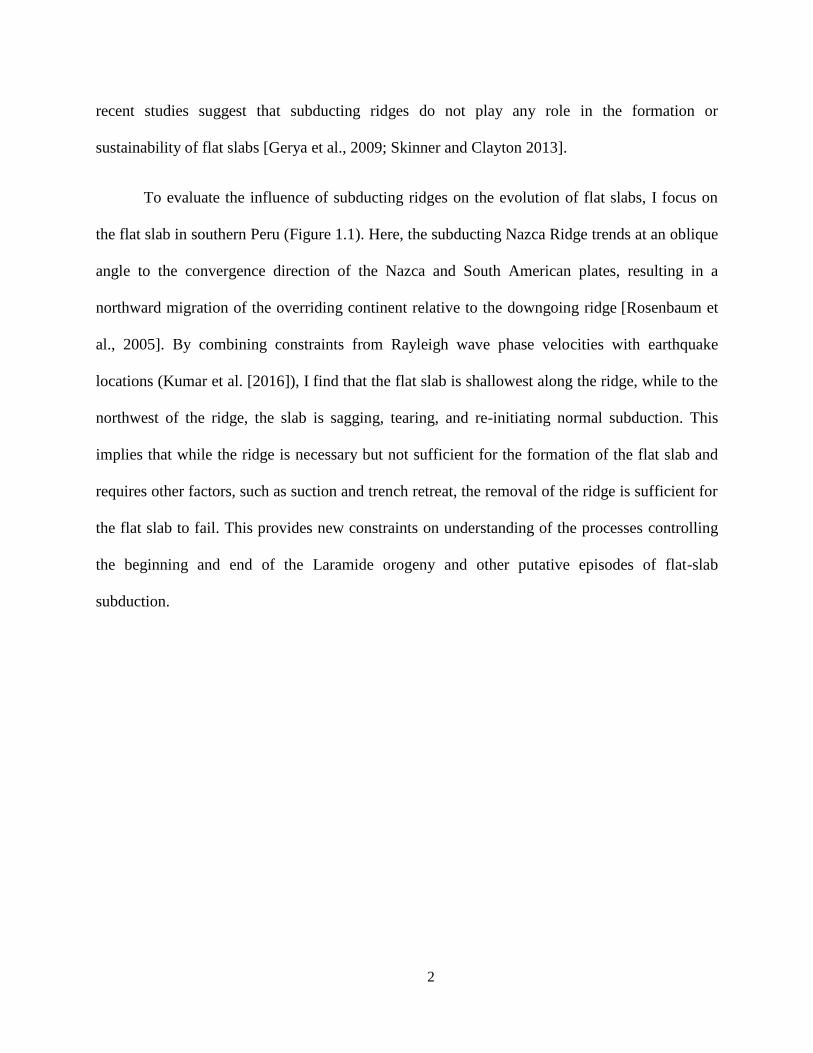
recent studies suggest that subducting ridges do not play any role in the formation or
sustainability of flat slabs [Gerya et al., 2009; Skinner and Clayton 2013].
To evaluate the influence of subducting ridges on the evolution of flat slabs, I focus on
the flat slab in southern Peru (Figure 1.1). Here, the subducting Nazca Ridge trends at an oblique
angle to the convergence direction of the Nazca and South American plates, resulting in a
northward migration of the overriding continent relative to the downgoing ridge [Rosenbaum et
al., 2005]. By combining constraints from Rayleigh wave phase velocities with earthquake
locations (Kumar et al. [2016]), I find that the flat slab is shallowest along the ridge, while to the
northwest of the ridge, the slab is sagging, tearing, and re-initiating normal subduction. This
implies that while the ridge is necessary but not sufficient for the formation of the flat slab and
requires other factors, such as suction and trench retreat, the removal of the ridge is sufficient for
the flat slab to fail. This provides new constraints on understanding of the processes controlling
the beginning and end of the Laramide orogeny and other putative episodes of flat-slab
subduction.

3
Figure 1.1 Reference map of the Peruvian flat-slab region, illustrating the subducting Nazca
Ridge beneath the advancing South American plate. Diamonds represent seismic stations used in
this study: orange, PULSE; dark red, CAUGHT; yellow, PERUSE; red, the permanent NNA
station. Yellow stars represent the cities Lima and Cusco. Red triangles represent volcanoes
active during the Holocene epoch. The black arrow indicates the relative motion of the South
American plate with respect to the Nazca Plate [Gripp and Gordon, 2002]. Dotted white lines
show the estimated position of the Nazca Ridge 12–10 Ma and today [Rosenbaum et al., 2005].
Map is produced using Generic Mapping Tools [Wessel & Smith, 2001].

4
1.2 Data processing
Data were collected from several seismic networks: PULSE (PerU Lithosphere and Slab
Experiment) [Eakin et al., 2014], CAUGHT (Central Andean Uplift and Geodynamics of High
Topography) [Ward et al., 2013], PERUSE (Peru Subduction Experiment) [Phillips and Clayton,
2014], and the global network permanent stations in Lima, Peru (Figure 1.1). The PULSE
seismic network consists of 40 three-component broadband seismometers, sampling at 40
samples per second, installed along three transects in central and southern Peru. The northern
transect extends between Lima and Satipo with an ~18 km station interval. The middle transect
extends from Pisco to Ayacucho with interstation distances varying from ~25 km to ~60 km. The
southern transect stretches from east of Nazca to beyond Cusco into the Amazon Basin, with a
station interval of ~15 km NE from Cusco, and ~40 km SW from Cusco. The dataset is
augmented with records from twelve adjacent CAUGHT stations [Ward et al., 2013] and eight
PERUSE stations [Phillips and Clayton, 2014] that improved the resolution along the southern
edge of the flat slab.

5
A fundamental mode of Rayleigh wave arrivals was analyzed for 65 well recorded
teleseismic events that occurred between October 2010 and June 2013. The events had
magnitudes ≥5.5 and epicentral distances beyond 25° from the center of the array (Figure 1.2).
Instrument responses were normalized and traces were further bandpassed using a Butterworth
filter, 7-10 mHz wide, centered on the frequency of interest. The fundamental mode of Rayleigh
wave was windowed for 12 periods in the band between 0.007 and 0.03 Hz and cut with a 50 s
cosine taper at either end (Figure 1.3). The width of the window varied with different events and
periods, but for particular period and event it was constant. Phases and amplitudes of waves for
each period at each station were later determined using Fourier analysis.
Figure 1.2 Events used in the study

6
1.3 Methods
1.3.1 Two-plane Wave Method
The finite frequency two-plane wave method has been employed to invert for Rayleigh
wave phase velocities [Forsyth and Li, 2005; Yang and Forsyth, 2006]. This method differs from
more traditional surface wave approaches by accounting for the scattering outside of the study
region which may cause Rayleigh waves to arrive off the great circle path. An incoming wave
field is modeled as a sum of two interfering plane waves, each presented with its amplitude,
phase, and backazimuth, which constructively or destructively interfere across the array. The
inversion consists of two steps. The first step solves for the 6 wave parameters for each event
using a grid search and assuming fixed velocities. To account for complexities caused by
Figure 1.3 Processed signal for different periods. The signal was recorded at station CP13
(71.44°W, 14.78°S).

7
heterogeneities within the study area, the model incorporates 2-D sensitivity kernels developed
by Yang and Forsyth [2006]. The calculations of kernels are based on the derivation of Zhou et
al. [2004] which incorporate the (Born) single scattering approximation. Using 2-D sensitivity
kernels for both amplitude and phase can significantly improve the spatial resolution [Yang and
Forsyth [2006].
The second step inverts for phase velocities based on differences between predicted and
calculated amplitudes and phases at each station. Phase velocities are approximated as
C(ω,θ) = B0(ω) + B1(ω)cos(2θ) + B2(ω)sin(2θ), (1.1)
where C is phase velocity at a specific frequency (ω) and backazimuth (θ), B0 is the isotropic
phase velocity term, while B1 and B2 refer to anisotropic terms. The higher order terms are
omitted, since they have been shown to be small for Rayleigh waves [Smith and Dahlen, 1973;
Weeraratne et al., 2007].
The phase velocity maps are constructed using linear weighting function of neighboring
grid points across the area with corners at 10°S and 18°S, and 69°W and 79°W (Figure 1.4). The
grid nodes are approximately equidistant at every quarter of a degree, and generated as a function
of azimuth and distance from the pole of rotation, which is set to be 90° relative to North from
the center of the array.
8
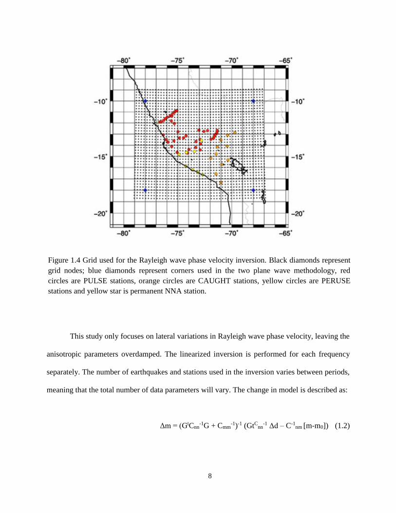
This study only focuses on lateral variations in Rayleigh wave phase velocity, leaving the
anisotropic parameters overdamped. The linearized inversion is performed for each frequency
separately. The number of earthquakes and stations used in the inversion varies between periods,
meaning that the total number of data parameters will vary. The change in model is described as:
Δm = (GtCnn-1G + Cmm
-1)-1 (GtCnn
-1 Δd – C-1nm [m-m0]) (1.2)
Figure 1.4 Grid used for the Rayleigh wave phase velocity inversion. Black diamonds represent
grid nodes; blue diamonds represent corners used in the two plane wave methodology, red
circles are PULSE stations, orange circles are CAUGHT stations, yellow circles are PERUSE
stations and yellow star is permanent NNA station.

9
where Cnn is an a priori data covariance matrix, and Cmm is model covariance matrix, set to 0.15
km/s for isotropic velocity terms. The choice of regularization parameters is always a tradeoff
between the amplitude of the model corrections and data misfit. Several values for isotropic
velocities were tested, ranging from 0.05 km/s to 0.5 km/s. Smaller values result in overdamped
inversions that reveal prominent features required by the data, but underestimate their
amplitudes. Larger values result in underdamped inversions that produce spurious features with
unreasonably large and rapidly varying amplitudes. To ensure a stable solution, the misfit
between predicted and observed phase velocities in the shear wave inversion was checked. Final
model uses 0.15 km/s for isotropic velocities, since the average root mean squared (r.m.s) phase
misfit between predicted and observed phase velocities in the shear wave inversion increases
rapidly at model covariance greater than this value (Figure S1.1).

10
The starting model consists of IASPEI91 mantle velocities and crustal velocities
developed by James [1971] for the Peruvian flat slab region (Figure 1.5). The crustal thickness is
highly variable in the study area, ranging from thin oceanic crust to ~70 km thick crust below the
high Andean peaks (Figure 1.6). Thus, a 2-D crustal thickness map was created using results
from Tassara et al.,[2006], smoothed along the coast, and used to adjust starting model
accordingly at each grid point in the inversion. Phase velocities were predicted across the study
region using forward algorithm of Saito [1988] and used as a starting model for the two-plane
wave inversion (Figure 1.7). The best resolved areas are beneath the Western Cordillera,
Altiplano, and Eastern Cordillera, while the resolution drops in the forearc and Sub-Andean zone

11
(Figure 1.8). The resolution within the foreland basin is mostly confined along the stations
deployed in foreland basin in eastern Peru.
Figure 1.5 Sensitivity kernels for periods used in the study with 1D starting shear wave velocity
model.
12
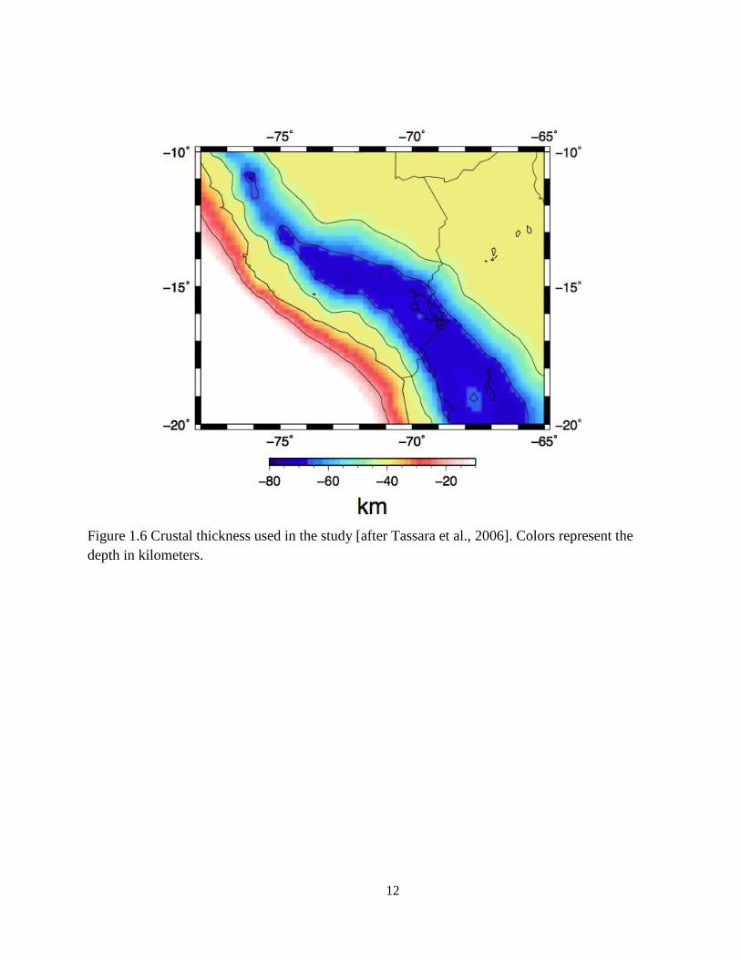
Figure 1.6 Crustal thickness used in the study [after Tassara et al., 2006]. Colors represent the
depth in kilometers.

13
Figure 1.7 Starting Rayleigh wave phase velocities. Colors and contours indicate absolute phase
velocities. Red triangles are Holocene volcanoes. Black rectangles, circles and stars are stations
used in the study.

14
1.3.2. Shear wave inversion
The obtained Rayleigh wave phase velocities were inverted for shear wave velocities
using forward algorithm of Saito [1988] and inverse algorithm of Weereratne et al. [2003].
Rayleigh wave phase velocities are sensitive to shear wave velocities at different depths,
depending on frequency. Sensitivity kernels (Figure 1.5) for longer periods are significantly
broader compared to shorter periods and sample greater depths.
The starting velocity model in the shear wave inversion was the same as the one to
predict phase velocities (Figure 1.5). The vertical resolution is affected by the thickness of
layers. Shear wave velocity columns were parameterized so that the diagonal value in the
resolution matrix for a particular layer ranges between 0.1 and 0.3. Figure 1.9 shows the
resolution matrix diagonal for each inverted node with average values for each layer. The
vertical resolution drops below 0.1 at depths shallower than ~40 km and greater than ~200-250
km (Figure 1.9).
Figure 1.8 Resolution for the 40 and 58 s periods. Resolution matrix diagonal for Rayleigh wave
phase velocities is indicated in grey scale. Red triangles are Holocene volcanoes. Black
rectangles, circles and stars are stations used in the study.

15
The model covariance obtained for phase velocities from the two-plane wave method was
used as data covariance to regularize the shear wave velocity inversion. The average root mean
square (RMS) misfit between predicted and observed phase velocities over all periods indicates
an average error of ~0.02 km/s (Figure 1.10).
Figure 1.9 Resolution matrix diagonal values for all 1D shear wave velocity inversions. Colors
of the circles indicate average R-values for each layer.
16
1.3.3 Resolution Tests
The main new features observed in this study include the far inboard extent of flat slab
along the subducting Nazca ridge and the slab tear north of the ridge. A range of tests were
performed to investigate lateral and vertical resolution to ensure the robustness of these features.
1.3.3.1. Lateral Resolution
The size of the resolution matrix for the isotropic model parameters is 1880 x 1880
(3,534,400). The resolution matrix rows of isolated model parameters for several periods were
plotted, with an emphasis on the spatial resolution at 3 locations along the northern profile north
of the subducting Nazca Ridge: one where I observe re-steepening of the slab, one at the slab
tear, and one along the flat slab remnant (Figure 1.11,Figure 1.12). In addition, points at 2
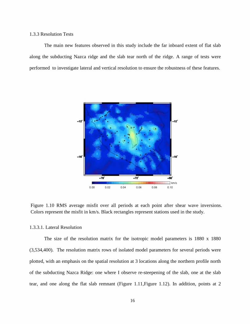
Figure 1.10 RMS average misfit over all periods at each point after shear wave inversions.
Colors represent the misfit in km/s. Black rectangles represent stations used in the study.
17
locations along the subducting Nazca Ridge were investigated: one referring to the observed far
inboard extent of the flat slab (“long flat slab”), and one where previous studies [Cahill and
Isacks, 1992] suggest the end of flat slab should be (“short flat slab”). The examination of
resolution matrix for these 5 selected nodes is primarily intended to demonstrate sufficient
spatial resolution to resolve the slab tear north of the ridge and the inboard extent of flat slab
along the ridge. The focus was on intermediate periods because they have peak sensitivity at the
most relevant depths (Figure 1.5). The tests show that these model parameters are able to resolve
spatial scale features smaller than those discussed in this study. The only node with a particularly
broad sensitivity cone is the one at the far inboard extent of the flat slab. This suggests that,
while the inboard extent of the flat slab may not be as well resolved as in other locations, a
shorter flat slab location would have been imaged accurately if it did exist. The inboard extent of
flat slab is therefore a conservative estimate.

18
Figure 1.11 Resolution kernels of isolated model parameters for period 58 s. Stars along
northernmost profile indicate locations where I observe re-steepening of the slab (i.), slab tear
(ii.) and flat slab remnant (iii.); while 2 stars along the subducting Nazca Ridge refer to
locations of proposed (greater) inboard extent along the Nazca ridge track (iv.) (“long flat
slab”) and a flat slab with shorter extent (v.) (“short flat slab”) previously suggested by Cahill
and Isacks [1992].
19
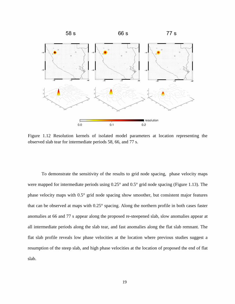
To demonstrate the sensitivity of the results to grid node spacing, phase velocity maps
were mapped for intermediate periods using 0.25° and 0.5° grid node spacing (Figure 1.13). The
phase velocity maps with 0.5° grid node spacing show smoother, but consistent major features
that can be observed at maps with 0.25° spacing. Along the northern profile in both cases faster
anomalies at 66 and 77 s appear along the proposed re-steepened slab, slow anomalies appear at
all intermediate periods along the slab tear, and fast anomalies along the flat slab remnant. The
flat slab profile reveals low phase velocities at the location where previous studies suggest a
resumption of the steep slab, and high phase velocities at the location of proposed the end of flat
slab.
Figure 1.12 Resolution kernels of isolated model parameters at location representing the
observed slab tear for intermediate periods 58, 66, and 77 s.

20
A series of checkerboard tests were performed using the surface wave resolution
matrices to test the size of the anomalies that can be recovered with varying periods used in this
study (Figure 1.14, Figure 1.15, Figure 1.16). These tests were aimed to show whether the spatial
resolution is sufficient to recover the size of the anomaly analogous to the observed tear and
whether the resolution is sufficient to resolve the inboard extent of flat slab. For this reason 5
selected nodes (shown in Figure 1.11, Figure 1.12, and Figure 1.13) were plotted. In addition,
these tests yield a better understanding of the spatial resolution of phase velocity maps across the
study area and easily reveal areas that suffer from smearing (due to preferential ray path
direction and/or lack of data). Short and intermediate periods, with peak sensitivities between 50
Figure 1.13 Phase velocity maps using 0.25° and 0.5° grid node spacing. Green circles refer to
nodes examined in Figure 1.11. Contour lines are absolute phase velocities and colors are
velocity deviations.

21
and 150 km depth, are able to recover smaller anomalies, equal to and smaller than the lateral
extent of the observed slab tear. The tests show sufficient spatial resolution to resolve the slab
tear, flat slab remnant to the east, and re-steepened slab to the west. Longer periods, which
mostly sample subslab material, can recover slightly larger features. However, both shorter and
longer periods are able to resolve the size of the anomaly analogous to subducting slab at the end
of the flat slab. These checkerboard tests demonstrate ability to resolve anomalies where
previous studies suggested the end of flat slab, while the node representing the far inboard extent
of flat slab may be streaked due to a lack of crossing rays. Thus, based on these tests it can be
can concluded with confidence that the inboard extent of flat slab along the subducting Nazca
Ridge is not where previously assumed, but further inboard. Resolution at the location
representing the far inboard extent of flat slab is weak and suffers from smearing. However,
conclusion on the far inboard extent of flat slab is supported by constraints from other studies:
the body wave tomography of Scire et al., [2016], and converted ScSp phases done by Snoke, J.
A., Sacks, I. S., & Okada, [1977].

22
Figure 1.14 Checkerboard tests estimated from resolution matrix for short periods (33 and 45 s).
Colors represent the recovered anomaly.

23
Figure 1.15 Checkerboard tests estimated from resolution matrix for intermediate periods (58
and 77 s). Colors represent the recovered anomaly.

24
Figure 1.16 Checkerboard tests estimated from resolution matrix for long periods (100 and 125 s).
Colors represent the recovered anomaly.

25
1.3.3.2 Vertical Resolution
The following tests examine the vertical resolution of the model. Figure 1.17
demonstrates ability to recover a dipping slab south of the ridge. I model a shear wave velocity
structure with a 70 km thick steeply dipping slab associated with a velocity of 4.6 km/s (Figure
1.17 (iv)). This model is based on my interpretations of the observed structures that are later
shown in Figure 1.17 d. I predict dispersion curves for this model using the code of Saito
[1988], add noise to predicted phase velocities, and invert them using the same starting model
(Figure 1.17 (ii)) and regularization parameters as for the model shown in Figure 1.17(iii). The
Gaussian noise was generated from misfits obtained in my final model using the Central Limit
Theorem Method and randomly assigned to predicted phase velocities. The steeply dipping
structure can be recovered, but its thickness appears greater due to vertical smearing. I was not
able to recover the full amplitude of the anomaly, but somewhat lower velocities (4.45 - 4.55
km/s). The model calculated using observed data (Figure 1.17 (iii)) indicates shear wave
velocities above 4.55 km/s. This recovery test suggests that, in order to fully recover the
amplitude of observed high shear wave velocities, the slab in Figure 1.17 (iv) either has shear
wave velocities greater than 4.6 km/s, or the thickness of the slab exceeds 70 km, or both.

26
Figure 1.17 Recovery tests for the dipping slab south to the ridge. (i) Map showing the
transect and stations used in the study (rectangles); (ii) starting model used in the shear wave
velocity inversion; contour lines and colors are absolute shear wave velocities, black inverted
triangles are stations, red triangles are Holocene volcanoes; (iii) model calculated using
observed data; (iv) model based on my interpretations of the observed structures; (v)
recovered model.

27
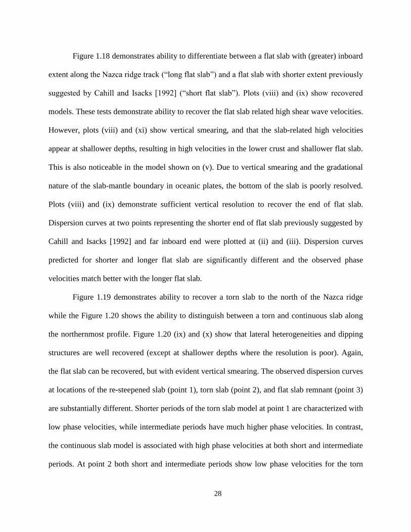
Figure 1.18 Recovery tests for the flat slab. (i) transect; (ii) dispersion curve at location
representing the shorter end of flat slab previously suggested by Cahill and Isacks [1992]; (iii)
dispersion curve at location representing the greater inboard extent of flat slab (proposed in this
study); error bars represent one standard deviation of uncertainty; (iv) starting model; (v) model
calculated using observed data; (vi) model with proposed (greater) inboard extent of flat slab;
(vii) model with shorter flat slab previously suggested by Cahill and Isacks [1992]; (viii)
recovered model from (vi); (ix) recovered model from (vii).
28
Figure 1.18 demonstrates ability to differentiate between a flat slab with (greater) inboard
extent along the Nazca ridge track (“long flat slab”) and a flat slab with shorter extent previously
suggested by Cahill and Isacks [1992] (“short flat slab”). Plots (viii) and (ix) show recovered
models. These tests demonstrate ability to recover the flat slab related high shear wave velocities.
However, plots (viii) and (xi) show vertical smearing, and that the slab-related high velocities
appear at shallower depths, resulting in high velocities in the lower crust and shallower flat slab.
This is also noticeable in the model shown on (v). Due to vertical smearing and the gradational
nature of the slab-mantle boundary in oceanic plates, the bottom of the slab is poorly resolved.
Plots (viii) and (ix) demonstrate sufficient vertical resolution to recover the end of flat slab.
Dispersion curves at two points representing the shorter end of flat slab previously suggested by
Cahill and Isacks [1992] and far inboard end were plotted at (ii) and (iii). Dispersion curves
predicted for shorter and longer flat slab are significantly different and the observed phase
velocities match better with the longer flat slab.
Figure 1.19 demonstrates ability to recover a torn slab to the north of the Nazca ridge
while the Figure 1.20 shows the ability to distinguish between a torn and continuous slab along
the northernmost profile. Figure 1.20 (ix) and (x) show that lateral heterogeneities and dipping
structures are well recovered (except at shallower depths where the resolution is poor). Again,
the flat slab can be recovered, but with evident vertical smearing. The observed dispersion curves
at locations of the re-steepened slab (point 1), torn slab (point 2), and flat slab remnant (point 3)
are substantially different. Shorter periods of the torn slab model at point 1 are characterized with
low phase velocities, while intermediate periods have much higher phase velocities. In contrast,
the continuous slab model is associated with high phase velocities at both short and intermediate
periods. At point 2 both short and intermediate periods show low phase velocities for the torn

29
slab model, but high phase velocities for the continuous slab model. At point 3 both short and
intermediate periods are associated with high phase velocities for both torn and continuous flat
slab. Generally, the observed dispersion curves can be reproduced with the model of torn slab,
except for the low phase velocities at shorter periods at point 1. This is because low shear
velocities were not introduced in the lower crust in the starting model. Dispersion curves for the
continuous flat slab differ from the observed at points 1 and 2, especially at intermediate periods
that sample upper mantle material.
Figure 1.19 Recovery tests for the tearing slab.(i) reference map; (ii) starting model; (iii) model
calculated using observed data; (iv) model based on the proposed torn slab; (v) recovered model.

30
Figure 1.20 Recovery tests for the re-steepened slab.(i) transect; (ii) dispersion curve at the re-
steepened slab; error bars represent one standard deviation; (iii) dispersion curve at location of
the slab tear; (iv) dispersion curve at location of the flat slab remnant; (v) starting model; (vi)
model calculated using observed data; (vii) model with the proposed slab tear; (viii) model
with continuous flat slab previously suggested by Cahill and Isacks [1992]; (ix) recovered
model from (vii); (x) recovered model from (viii).

31
1.4 Results and discussion
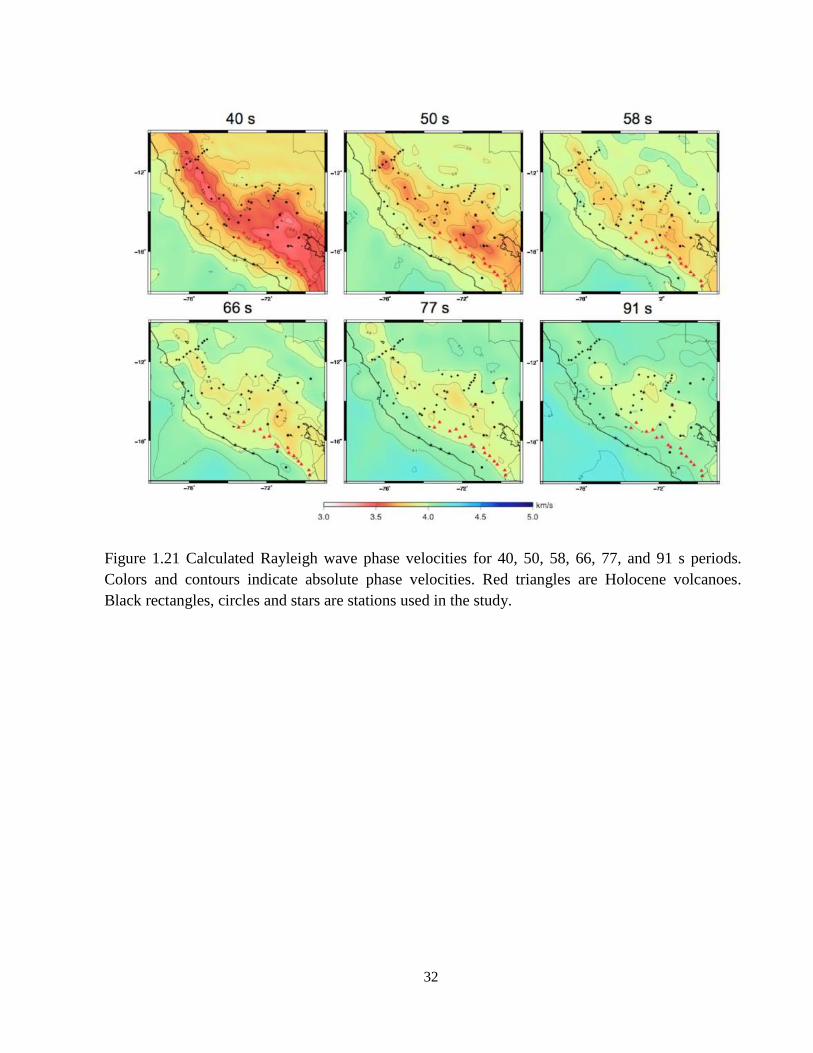
The results of Rayleigh wave phase velocity and shear wave inversions are presented in
Figure 1.21; the results of the shear wave inversion are shown in Figure 1.22 and Figure 1.23.
These tomographic images, in conjunction with the improved earthquake relocations of Kumar et
al., [2016] show the flat slab to be shallowest along the present-day projected location of the
subducted Nazca Ridge (Figure 1.23 g). To the south (Figure 1.23h), the slab transitions abruptly
from flat to normal, and earthquake locations align with an observed high shear wave velocity
anomaly. To the north, where previous studies have proposed a broad flat slab of relatively
uniform depth [Cahill and Isacks,1992; Hayes et al., 2012], earthquake distribution shows a
gradual but marked deepening of the Wadati-Benioff zone (Figure 1.23 e-f). To the east, high
shear wave velocities associated with the flat slab extend significantly further inboard than the
seismically active portion of the plate (Figure 1.23 g). The downward bend in the high velocity
plate at the inboard extent of the flat slab appears to coincide with the location of the trench at
~10 Ma [Rosenbaum et al., 2005].
32
Figure 1.21 Calculated Rayleigh wave phase velocities for 40, 50, 58, 66, 77, and 91 s periods.
Colors and contours indicate absolute phase velocities. Red triangles are Holocene volcanoes.
Black rectangles, circles and stars are stations used in the study.

33
Of particular note is the geometry of the subducted plate north of the projected Nazca
Ridge track (Figure 1.23 a, b, c, e, f). Here, a dipping high velocity anomaly can be observed
trenchward of a dipping low velocity anomaly. There are strong similarities between these
Figure 1.22 Shear wave velocity maps at 70, 95, 125, and 165 km depth. Colors represent velocity
deviations with respect to the reference model (Figure 1.5), while contours show absolute
velocities. Green stars indicate earthquakes within 20 km depth relocated by Kumar et al., [2016]
using HypoDD [Waldhauser and Ellsworth, 2002]. Red triangles represent Holocene volcanoes.
Black rectangles, circles and stars are stations used in the study.

34
structures (in an area previously believed to comprise typical flat slab) and those observed to the
south beneath the active arc (Figure 1.23 e-f). These structures differ from those observed
adjacent to the ridge, where the continuous flat slab is well resolved (Figure 1.23 e-f; Figure 1.23
g). I interpret the westward-dipping trench-parallel low velocity region to be evidence of
asthenosphere between two torn portions of subducted plate. The dipping high velocity anomaly
to the west indicates the presence of a normally dipping slab extending to at least 200 km depth.
This is consistent with the location of scatterers identified in earlier studies of ScSp phases
[Hasegawa and Sacks, 1980]. The subhorizontal seismicity to the east of the tear that aligns with
high shear wave velocities illuminates a remnant flat slab that has not yet been fully subducted.
Local shear wave splitting studies show trench parallel fast directions that align with low
velocities in the model [Eakin et al., 2014], consistent with north-south directed asthenospheric
flow through a break in the Nazca plate. This low velocity anomaly collocates with the localized
high heat flow measured at the surface (196mW/s²) [Uyeda et al., 1980] (Figure 1.23e). Along
the northernmost transect the location of the slab is not well resolved above ~100 km depth
(Figure 1.23e). Using ambient noise tomography may help to resolve the slab geometry here by
providing improved constraints on velocities at shallower depths.

35
Figure 1.23 Shear wave velocities and seismicity at 75, 105, and 145 km depth and transects along
the northern re-initiating steep slab (A-A’, B-B’), flat slab (C-C’) and southern steep slab segments
(D-D’). Colors indicate velocity deviations dVs/Vs (%), contours show absolute velocities. (a), (b),
(c) Black circles represent stations used in the study; red triangles are Holocene volcanoes; green
stars are earthquakes within 20 km of the depth shown [from Kumar et al., 2016]; black lines refer
to cross-sections shown in (e), (f), (g), and (h). The grey dashed line refers to the location of the
trench 10 Ma [Rosenbaum et al., 2005]. The black dashed line (“T”) in (b) and (c) indicates the
location of the slab tear; R refers to the resumption of steep subduction at the eastern edge of the
flat slab. (d) The inferred flat slab geometry along the Nazca Ridge track and slab tear north of the
ridge. (e-h) Black dots show earthquake locations from this study, black inverted triangles are
stations, red triangles are Holocene volcanoes, and the orange triangle represents the location of an
unusually high heat flow measurement [Uyeda et al., 1980]. Dashed lines show the inferred top of
the slab. The crustal thickness is shown with a thick black line in each cross-section.

36
By combining this shear wave velocity model, relocated earthquakes [Kumar et al.,
2016], and previous geodynamic modeling studies, Antonijevic et al. [2015] propose temporal
evolution of the Peruvian flat slab, which combines the influences of trench retreat/overriding
plate motion, suction, and ridge buoyancy (Figure 1.24). It assumes that the combination of all
three forces is necessary for the formation of the flat slab, but that the first two are sufficient to
perpetuate the flat slab after the departure of the ridge. A comparison between the conceptual
model’s slab geometry at present (Figure 1.24 g) with actual (observed) slab geometry (Figure
1.24h) allows to test these assumptions. The abrupt edge of the flat slab that is observed south of
the ridge is very similar to that proposed by the conceptual model [Antonijevic et al., 2015]. The
dominant model principle controlling the geometry of the flat slab here is the effect of ridge
buoyancy, since there is no difference in trench rollback or continental lithospheric structure that
might affect suction along strike in this region. Observations therefore support the necessary
contribution of the ridge to the formation of flat slabs, but are also not inconsistent with
additional contributions from suction and trench rollback.

37
Figure 1.24 Proposed evolution of the Peruvian Flat Slab [from Antonijevic et al., 2015]. Panels
a-f show proposed contours of the subducted slab, assuming that the ridge remains buoyant for
10 Ma after entering the trench. The approximate location of the subducted ridge is denoted by
the black rectangular outline. Brown areas show areas of the continent underlain by flat slab at
each time step. Triangles indicate volcanoes active during the 2 Ma following the time of the
frame shown [INGEMMET, Peru 2014]. The location of the South American continent relative
to the Nazca Ridge follows Rosenbaum et al., [2005]. a) The proposed reflected location of the
conjugate to the Nazca Ridge in yellow [Rosenbaum et al., 2005]. e) Red triangles: volcanism
from 3-2 Ma, brown triangles: volcanism for 2-1 Ma. f) Volcanism for 1 to 0 Ma (not including
Holocene volcanism). g) Modern seismicity from the present study with depths >50 km, and
contours as they would be if the removal of the ridge did not affect the longevity of the flat slab.
h) Modern seismicity [Kumar et al, 2016] and local seismicity > 50 km depth [ISC, 2012]. The
slab contours are based on earthquake locations of Kumar et al, [2016] and the location of high
velocity anomalies in tomographic results. Dashed lines indicate contours that are less certain.
The pink triangular shape may indicate a slab window caused by tearing.

38
Differences between the observed slab geometry and the geometry derived from
conceptual model are visible to the north of the ridge. In this area, the effect of the ridge is no
longer present, and the geometry of the flat slab in the conceptual model [Antonijevic et al.,
2015] is controlled by the effects of suction and trench rollback alone. While both the conceptual
model and observations indicate a flat slab that broadens to the northwest of the ridge, the
detailed morphologies are very different. In addition to an overall deepening of the flat slab north
of the ridge (Figure 1.24 g,h), a clear trench parallel break can be observed in the subducted plate
and a resumption of normal subduction trenchward of this tear (Figure 1.24 a-c, Figure 1.24h).
This strongly suggests that, in spite of the presence of suction and trench rollback, the flat slab is
no longer stable once the buoyant Nazca Ridge has been removed. Furthermore, once a break is
present, the newly subducted plate assumes a normal steep dip angle, rather than a flat slab
geometry. This study is not able to resolve the northern extent of the Peruvian flat slab, nor can it
establish the along-strike extent of the tear. However, ISC catalog locations north of the study
area show a gap in seismicity that may be consistent with the absence of a flat slab due to a
progressively tearing plate (Figure 1.24 h) [ISC, 2012]. The northward extent of the flat slab east
of the tear may be due in part to the subduction of the Inca Plateau [Gutscher et al., 1999],
though this is beyond the scope of the present study.
This model is applicable to all flat slab geometries where a distinct change of dip angle is
observed. This change in dip occurs at the depth at which the slab becomes neutrally buoyant.
These results may not be applicable to slabs where the dip angle is constant but very shallow
[Skinner and Clayton, 2013] (e.g. Alaska, Cascadia). Shallowly dipping slabs sink at a constant
rate, which is inconsistent with a period of neutral buoyancy. Shallowly dipping slabs may have
some similar consequences as flat slabs, though notably they do not result in a complete

39
cessation of arc volcanism (as occurred during the Laramide and is observed in Peru today), only
its inboard deflection.
These results may provide important insights into the final stages of flat slab subduction.
Previous studies use volcanic patterns to reconstruct the formation and foundering of the
Farallon flat slab [Humphreys et al., 2003; Liu et al., 2010; Jones et al., 2011]. The diversity of
models for the progression of this foundering is indicative of the insufficiency of the constraints
provided by volcanic trends alone. These results suggest that once the flat slab extends some
distance away from the buoyant feature, it will begin to sink and/or tear. The tearing of the
Farallon plate due to excessive flat slab width may be consistent with tomographic images of
broken fragments of the Farallon plate [Sigloch, McQuarrie and Nolet, 2008].
1.5 Conclusion
New tomographic images in conjunction with relocated earthquakes [Kumar et al., 2016]
reveal the complex geometry of the subducting Nazca Plate in Southern Peru, providing insights
into the temporal evolution of flat slabs from initial shallowing to collapse [Antonijevic et al.,
2015]. These results show that the flat slabs form due to a combination of trench retreat, suction,
and the inability of over-thickened oceanic crust to sink below some depth (~90 km) until
sufficiently eclogitized to once again become negatively buoyant. Flat slabs that extend laterally
beyond some critical distance from the buoyant over-thickened crust will begin to founder, even
in the presence of other factors such as suction and trench retreat. The Peruvian flat slab yields
new constraints for the reconstruction of flat slab genesis and the nature of the flat slab
foundering.

40
REFERENCES
1. Antonijevic, S. K., Wagner, L. S., Kumar, A., Beck, S. L., Long, M. D., Zandt, G., Tavera,
H. & Condori, C. (2015). The role of ridges in the formation and longevity of flat slabs.
Nature, 524(7564), 212-215. doi:10.1038/nature14648.
2. Arrial, P. A., & Billen, M. I. Influence of geometry and eclogitization on oceanic plateau
subduction. EPSL, 363, 34-43 (2013).
3. Bedle, H., & van der Lee, S. Fossil flat-slab subduction beneath the Illinois basin,
USA. Tectonophysics, 424(1), 53-68 (2006).
4. Cahill, T., & Isacks, B. L. Seismicity and shape of the subducted Nazca plate. J. Geophys.
Res: Solid Earth. (1978–2012), 97(B12), 17503-17529 (1992). doi: 10.1029/92JB00493
5. Eakin, C. M., Long, M. D., Beck, S. L., Wagner, L.S., Tavera, H. & Condori, C. (2014).
Response of the mantle to flat slab evolution: Insights from local S splitting beneath Peru. J.
Geophys. Res. 41(10), 3438-3446 (2014). doi:10.1002/2014GL0599443
6. Forsyth, D. W., and Li, A. Array analysis of two-dimensional variations in surface wave
phase velocity and azimuthal anisotropy in the presence of multipathing interference. In:
Levander, A. Nolet, G. (Eds), Seismic Earth: Array of broadband seismograms, Geophysical
Monograph Series 157, 81-98 (2005). doi:10.1029/157GM06
7. Gerya, T. V., Fossati, D., Cantieni, C., & Seward, D. Dynamic effects of aseismic ridge
subduction: numerical modelling. Eur. J. Mineral. 21(3), 649-661 (2009).
8. Gripp, A. E., & Gordon, R. G. Young tracks of hotspots and current plate velocities. GJI.
150(2), 321-361 (2002). doi:10.1046/j.1365-246X.2002.0167.x
9. Gutscher, M. A., Olivet, J. L., Aslanian, D., Eissen, J. P., & Maury, R. (1999). The “lost Inca
Plateau”: cause of flat subduction beneath Peru?. Earth and Planetary Science Letters,
171(3), 335-341.
10. Hasegawa, A., & Sacks, I. S. Subduction of the Nazca plate beneath Peru as determined from
seismic observations. J. Geophys. Res.: Solid Earth. (1978–2012), 6(B6), 4971-4980 (1981).
11. Hayes, G. P., Wald, D. J., & Johnson, R. L. Slab 1.0: A three‐dimensional model of global
subduction zone geometries. J. Geophys. Res.: Solid Earth. (1978–2012), 117(B1) (2012).
12. Humphreys, E., Hessler, E., Dueker, K., Farmer, G. L., Erslev, E., & Atwater, T. How
Laramide-age hydration of North American lithosphere by the Farallon slab controlled
subsequent activity in the western United States. Int. Geol. Rev. 45(7), 575-595 (2003).
13. Instituto Geológico Minero y Metalúrgico – INGEMMET, On-line Catalog,
http://www.ingemmet.gob.pe, Peru (2014).
14. International Seismological Centre, On-line Bulletin, http://www.isc.ac.uk, Internatl. Seis.
Cent., Thatcham, United Kingdom (2012).

41
15. James, D. E. Andean crustal and upper mantle structure. J. Geophys. Res., 76(14), 3246-3271
(1971).
16. Jones, C. H., Farmer, G. L., Sageman, B., & Zhong, S. Hydrodynamic mechanism for the
Laramide orogeny. Geosphere, 7(1), 183-201 (2011).
17. Kennett, B.L.N. IASPEI 1991 Seismological Tables. Bibliotech, Canberra, Australia (1991).
18. Kumar, A., Wagner, L. S., Beck, S. L., Long, M. D., Zandt, G., Young, B., Tavera, H. &
Minaya, E. (2016). Seismicity and state of stress in the central and southern Peruvian flat
slab. Earth and Planetary Science Letters, 441, 71-80.
19. Liu, L., Gurnis, M., Seton, M., Saleeby, J., Müller, R. D., & Jackson, J. M. The role of
oceanic plateau subduction in the Laramide orogeny. Nature Geoscience, 3(5), 353-357
(2010).
20. Manea, V. C., Pérez-Gussinyé, M., & Manea, M. Chilean flat slab subduction controlled by
overriding plate thickness and trench rollback. Geology 40(1), 35-38 (2012).
21. Phillips, K., & Clayton, R. W. Structure of the subduction transition region from seismic
array data in southern Peru. Geophys. J. Int. ggt504 (2014).
22. Rosenbaum, G., Giles, D., Saxon, M., Betts, P. G., Weinberg, R. F., & Duboz, C. Subduction
of the Nazca Ridge and the Inca Plateau: Insights into the formation of ore deposits in Peru.
Earth and Planet. Sci. Lett. 239(1), 18-32 (2005).
23. Saito, M. DISPER80: a subroutine package for the calculation of seismic normal mode
solutions. In: Doornbos, D.J. (Ed.), Seismological Algorithms: Computational Methods and
Computer Programs. Elsevier, 293–319 (1988).
24. Scire, A., Zandt, G., Beck, S., Long, M., Wagner, L., Minaya, E., & Tavera, H. (2016).
Imaging the transition from flat to normal subduction: variations in the structure of the Nazca
slab and upper mantle under southern Peru and northwestern Bolivia. Geophysical Journal
International, 204(1), 457-479.
25. Snoke, J. A., Sacks, I. S., & Okada, H. Determination of the subducting lithosphere boundary
by use of converted phases. BSSA, 67(4), 1051-1060 (1977).
26. Sigloch, K., McQuarrie, N., & Nolet, G. Two-stage subduction history under North America
inferred from multiple-frequency tomography. Nature Geoscience, 1(7), 458-462 (2008).
27. Skinner, S. M., & Clayton, R. W. The lack of correlation between flat slabs and bathymetric
impactors in South America. Earth and Planet. Sci. Lett. 371, 1-5 (2013).
28. Smith, M. L., & Dahlen, F. A. (1973). The azimuthal dependence of Love and Rayleigh
wave propagation in a slightly anisotropic medium. Journal of Geophysical Research, 78(17),
3321-3333.

42
29. Tassara, A., Go ̈tze, H.J., Schmidt, S. & Hackney, R., 2006. Three-dimensional density
model of the Nazca plate and the Andean continental margin, J. Geophys. Res., 111,
doi:10.1029/2005JB003976.
30. Uyeda, S., Watanabe, T., Ozasayama, Y., & Ibaragi, K. Report of heat flow measurements in
Peru and Ecuador. Bull. Of the Earthquake Res. Institute 55, 55-74 (1980).
31. van Hunen, J., Van Den Berg, A. P., & Vlaar, N. J. On the role of subducting oceanic
plateaus in the development of shallow flat subduction. Tectonophysics 352(3), 317-333
(2002).
32. Vogt, P. R.. Subduction and aseismic ridges. Nature, 241, 189-191 (1973).
33. Waldhauser, F., W. L. Ellsworth. A Double-Difference Earthquake Location Algorithm:
Method and Application to the Northern Hayward Fault, California, Bull. Seismol. Soc. Am.
90, 1353-1368 (2000).
34. Ward, K. M., Porter, R. C., Zandt, G., Beck, S. L., Wagner, L. S., Minaya, E., & Tavera, H.
Ambient noise tomography across the Central Andes. Geophys. J. Int. 194(3), 1559-1573
(2013). Jones, C. H., Farmer, G. L., Sageman, B., & Zhong, S. Hydrodynamic mechanism for
the Laramide orogeny. Geosphere, 7(1), 183-201 (2011).
35. Weeraratne, D. S., Forsyth, D. W., Fischer, K. M., & Nyblade, A. A. Evidence for an upper
mantle plume beneath the Tanzanian craton from Rayleigh wave tomography. J. Geophys.
Res.: Solid Earth. (1978–2012), 108(B9) (2003).
36. Wessel, P., & Smith, W. H. (2001). The Generic Mapping Tools. 2013-01-01]. http://gmt.
soest. hawaii. edu.
37. Yang, Y., Forsyth, D. W. Regional tomographic inversion of the amplitude and phase of
Rayleigh waves with 2-D sensitivity kernels. Geophys. J. Int. 166, 1148-1160 (2006).
38. Zhou, Y., Dahlen, F. A., & Nolet, G. Three-dimensional sensitivity kernels for surface wave
observables. Geophys. J. Int. 158(1), 142-168 (2004).

43
CHAPTER 2: EFFECTS OF CHANGE IN SLAB GEOMETRY ON THE MANTLE FLOW
AND SLAB FABRIC IN SOUTHERN PERU2
2.1 Introduction
The subduction zone in southern Peru is characterized by the complex geometry of the
descending oceanic Nazca Plate that changes from steep to flat at ~16° S [Cahill and Isacks,
1992]. Along the flat slab segment, the ~40-45 Ma old Nazca plate [Müller et al., 2008] starts to
subduct at a normal dip angle to ~90 km depth. It then bends and continues almost horizontally
for several hundred kilometers beneath the South American continent (Figure 2.1).
Earlier studies recognized the spatial correlation between the flat slab and the subducting
Nazca Ridge [Gutscher et al., 2000]. The ridge was formed as a hotspot track either of the Easter
plume while the plume was still sufficiently close to the East Pacific Rise [Steinberger et al.
2002], or near Salas y Gomez, ~400 km further east [Ray et al. 2012]. The oceanic crust of the
ridge is considerably thickened with an ~5 km thick basaltic oceanic crust above an ~12 km thick
gabbroic layer [Hampel et al., 2004, Couch and Whitsett, 1981; Machare and Ortlieb, 1992]. Due
to the oblique orientation of the ridge with respect to the convergence direction [DeMets et al,
2010] (Figure 2.1), the ridge was located significantly further north (at ~11.2°S) when it started
to subduct ~11 Ma [Hampel et al., 2002; Rosenbaum et al., 2005]. While the combination of
several factors such as trench retreat, suction, and ridge subduction acted together to form the flat
______________________________________ 2 This chapter is under review in the Journal of Geophysical Research: Solid Earth. The original citation is:
Antonijevic, S. K., Wagner, L. S., Beck, S. L., Long, M. D., Zandt, G., Tavera, H. Effects of Change in Slab
Geometry on the Mantle Flow and Slab Fabric in Southern Peru.
44
slab, the removal of the ridge, as it moved too far south over time, caused the flat slab to fail to
the north [Antonijevic et al. 2015] (Figure 2.1). In contrast, along the southern edge of the flat
slab the descending plate is still continuous, but sharply contorted [Dougherty and Clayton,
2014; Phillips and Clayton, 2014; Ma and Clayton, 2014].
Seismic anisotropy is often used to better understand current and/or past deformation
patterns within the mantle [Long and Becker, 2010]. Typically, the crystallographic preferred
orientation (CPO) of olivine is invoked to explain the seismic anisotropy within the upper
mantle. Constraints from laboratory experiments and natural samples have led to the
development of simple rules of thumb for relating seismic anisotropy directions to mantle flow
directions [Karato et al., 2008]. These simplified relationships are useful in developing general
interpretations of seismic anisotropy data; however, they obscure potential complications due to
mantle flow fields that vary in space and time, as well as the complexities of CPO development,
particularly in settings such as a subduction zone [e.g., Skemer et al., 2012; Faccenda and
Capitanio, 2013; Di Leo et al., 2014; Skemer and Hansen, 2016].
45
Based on SKS splitting, Russo and Silver [1994] reported trench-parallel fast directions
along the Central Andean subduction zone. Their explanation for this anisotropic pattern is the
formation of CPO of olivine due to trench parallel mantle flow beneath the subducting slab,
which in turn is induced by trench rollback. Recent shear wave splitting studies, however, have
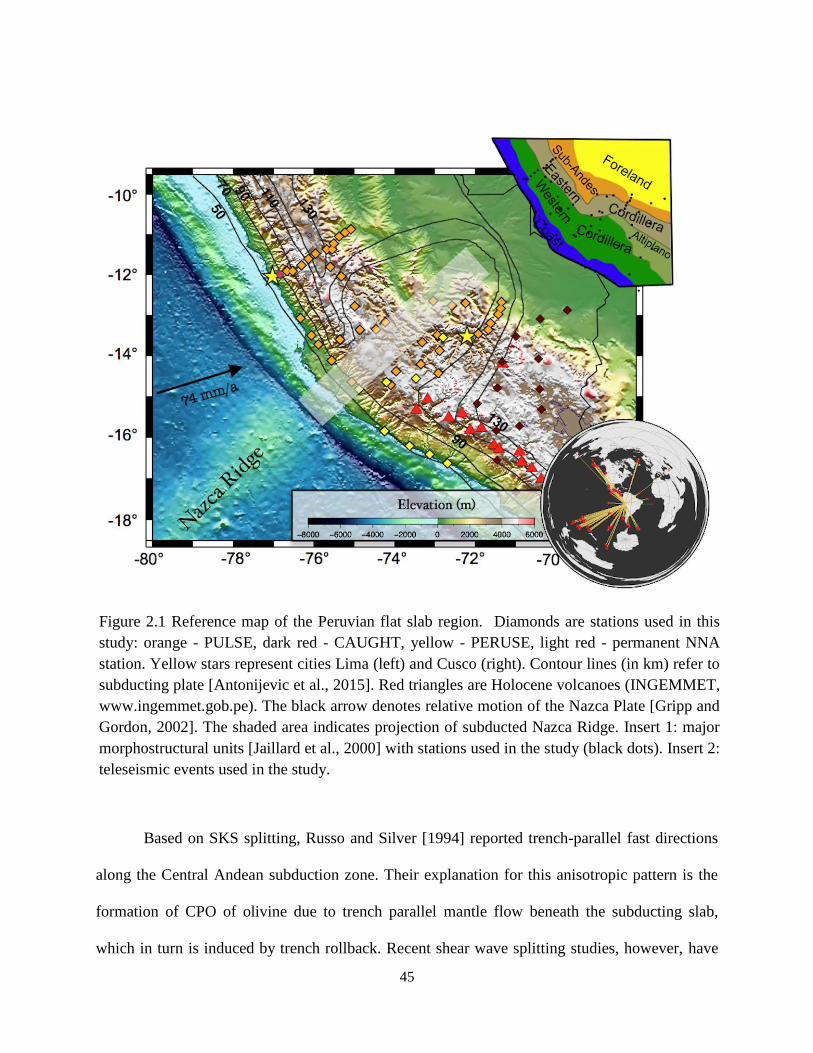
Figure 2.1 Reference map of the Peruvian flat slab region. Diamonds are stations used in this
study: orange - PULSE, dark red - CAUGHT, yellow - PERUSE, light red - permanent NNA
station. Yellow stars represent cities Lima (left) and Cusco (right). Contour lines (in km) refer to
subducting plate [Antonijevic et al., 2015]. Red triangles are Holocene volcanoes (INGEMMET,
www.ingemmet.gob.pe). The black arrow denotes relative motion of the Nazca Plate [Gripp and
Gordon, 2002]. The shaded area indicates projection of subducted Nazca Ridge. Insert 1: major
morphostructural units [Jaillard et al., 2000] with stations used in the study (black dots). Insert 2:
teleseismic events used in the study.
46
found more complex patterns across southern Peru. Results of local shear wave splitting reveal
predominantly trench-parallel alignments of fast directions north of the subducting ridge and
heterogeneous anisotropic patterns south of the ridge [Eakin et al., 2014]. Shear wave splitting
analyses of SKS, sSKS, and PKS phases between 10° and 18°S illuminate distinct spatial
variations along strike, where the projected subducting Nazca Ridge again marks a sharp
boundary in the anisotropic patterns [Eakin et al. 2015]. Multi-layered anisotropy characterized
by sub-slab trench-normal and supra-slab trench-parallel fast directions has been reported north
of the ridge [Eakin and Long, 2013], while the ridge track is associated with generally little or no
splitting of SKS phases [Eakin et al. 2015].
Complex patterns of seismic anisotropy have been observed in other subduction zones
worldwide. Often, these are associated with unusual slab geometry. Examples include the narrow
flat slab in central Chile/Argentina [Anderson et al., 2004], the torn slab in northern Colombia
[Porritt, Becker and Monsalve, 2014], and the slab edge present in Kamchatka [Peyton et al.,
2001]. The complexity of these various tectonic settings demonstrates the need for 3D
constraints on mantle flow and slab dynamics in these areas. Here I combine Rayleigh wave
anisotropy with 3D shear wave velocity structure to investigate mantle flow and slab fabric in
southern Peru. Unlike shear wave splitting, Rayleigh waves at different periods provide
constraints on the depth of the observed anisotropy that are otherwise difficult to attain. I find
that slab tear north of the projected Nazca Ridge creates a new pathway for mantle flow between
the region above the recently torn slab to the north and area below the flat slab to the south. This
lateral mantle flow may contribute to the low shear wave velocities I observe beneath the inboard
easternmost corner of the flat slab. I find evidence for modified slab fabric along the southern
edge of the flat slab, consistent with previous results and interpretations of Eakin et al. [2016],

47
but preserved fossil spreading fabric within the torn slab to the north. The contrast in slab fabric
along the strike supports the hypothesis that the extension due to change in slab geometry from
steep to flat may alter the internal slab anisotropy upon subduction.
2.2 Data
Data were collected from several seismic networks: PULSE (PerU Lithosphere and Slab
Experiment), CAUGHT (Central Andean Uplift and Geodynamics of High Topography),
PERUSE (Peru Subduction Experiment), and the Global Seismic Network permanent stations in
Lima, Peru (Figure 2.1). I used teleseismic events with magnitudes greater than 6.2 that occurred
during the PULSE deployment between 25° and 125° from the center of the array. Most of these
events come from the SW direction (from the Kermadec-Tonga subduction zone) and NNW
(from the Alaska subduction zone) (Figure 2.1, insert 2). To ensure a more heterogeneous back-
azimuthal coverage, events from over-sampled back-azimuths were limited and smaller but well
recorded events (M<6.2) coming from less represented directions were added (Figure 2.1, insert
2; Figure 2.2; (Figure S2.1). Well-recorded earthquakes with magnitudes greater than 8 and
epicentral distances beyond 125° from the center of the array were also included. The data are
further processed following the procedure described earlier in Chapter 1.

48
2.3 Methods
Two-plane wave method (Forsyth and Li [2005] and Yang and Forsyth [2006]),
described in Chapter 1, was used to invert for Rayleigh wave phase velocities. These inversions
also include anisotropy. The fast propagation direction can be calculated as
0.5*arctan(B2/B1) (2.1)
Figure 2.2 Rose diagrams showing back-azimuthal distribution of the events used in the study.

49
while the peak-to-peak anisotropy magnitude is represented as
2*(B1² + B2²)½ (2.2)
where B1 and B2 represent the anisotropic coefficients (see Equation 1.1). Grid nodes are
approximately equidistant and are generated as a function of azimuth and distance from a pole of
rotation, located 90° North of the center of the array [see Forsyth and Li, 2005 for further
details]. 0.33° grid node spacing for isotropic and 0.66° for anisotropic terms was used. Starting
Rayleigh wave phase velocities are important for a stable inversion. I use the same starting
model as the one described in Chapter I. The inversion is regularized with a model covariance,
set to 0.15 km/s for isotropic velocities (discussed in Chapter I) and 0.05 for anisotropic terms.
The obtained Rayleigh wave phase velocities are further inverted for shear wave velocities using
the algorithm of Saito [1988] and Weereratne et al. [2003] (Figure S2.2).
2.4 Results
2.4.1 Shear wave velocity model
The main differences between the new shear wave velocity model and the model
presented by Antonijevic et al. [2015] and in Chapter I include improved azimuthal distribution
of the teleseismic events used in the study and taking into account anisotropy in the phase
velocity maps, which may change the isotropic solution. However, these results reveal very
similar structures as previously reported by Antonijevic et al., [2015] (Figure 2.3, Figure S2.2).
North of the projected subducted Nazca Ridge a dipping high velocity anomaly coincides with
the location of a scatterer identified in earlier studies of ScSp phases [Snoke, Sacks, and James,
1979] (Figure 2.3d). The dipping high shear wave velocities are overlain by a dipping low
velocity anomaly. The low velocity anomaly is located beneath an unusually high heat flow
measurement (196mW/s²) [Uyeda et al., 1980]. The structures are consistent with a previously

50
proposed slab tear and the warm asthenospheric corner flow above the now normally dipping
slab to the west [Antonijevic et al., 2015] (Figure 2.3a-d).
Along the projected Nazca Ridge I observe an increase in shear wave velocities from
~4.4. km/s near the trench to > 4.55 km/s ~100-~150 km away from the trench, where the plane
of seismicity roughly illuminates the top of the slab (Figure 2.3e). However, the observed high
velocities continue much further inboard than the plane of seismicity and start to dip ~600-~680
km away from the trench. The feature is consistent with the previously proposed flat slab that
resumes steep subduction far to the east [Antonijevic et al., 2015]. Below the observed high
velocities, beneath the southeastern corner of the flat slab, I observe a pronounced low velocity
anomaly. At long periods (77-111s) I observe prominent low velocities centered at ~72.5°W
~13°S, with the greatest phase velocity reduction (~5%) at 91s (Figure 2.4). In the shear wave
velocity model, the low velocities first appear at ~125km depth. Velocities decrease with
increasing depth up to ~145 km where Vs approaches 4.2 km/s (Figure 2.3c,e, Figure 2.4). By
~165 km depth the anomaly shifts east and becomes less pronounced; by ~200 km depth
velocities increase above 4.4 km/s, but the resolution starts to decrease (Figure 1.9). This feature
is consistent with the observations of Scire et al. [2016], who also found significant velocity
reductions beneath the Peruvian flat slab using finite frequency teleseismic P- and S-wave
tomography.

51
Figure 2.3 Shear wave velocity maps at 75 (a), 105 (b), and 145(c) km depth and profiles along
the slab tear observed to the north (d), flat slab along the subducting Nazca Ridge (e), and steeply
subducting slab to the south (f). Colors represent velocity deviations with respect to the reference
model (Figure 1.5), while contours show absolute velocities. Black dots show earthquake
locations [from Antonijevic et al., 2015], black inverted triangles are stations, red triangles are
Holocene volcanoes, and the orange triangle (d) represents the location of an unusually high heat
flow measurement [Uyeda et al., 1980]. LVZ refers to low velocity anomaly discussed in the
text.

52
To the south, a progressive change in the dip of the slab from flat to steep can be
observed. These observations are consistent with a continuously contorted slab as reported in
previous studies [Dougherty and Clayton, 2014; Phillips and Clayton, 2014; Ma and Clayton,
Figure 2.4 Shear wave velocity maps at 125, 145, 185, and 205 km depth with transects shown in
Figure 2.3. Colors represent velocity deviations with respect to the reference model (Figure 1.5),
while contours show absolute velocities. Black inverted triangles are stations used in the study,
red triangles are Holocene volcanoes.

53
2014]. At ~17°S I observe high shear wave velocities aligned with the 30° dipping plane of
seismicity (Figure 2.3f). Above the high velocities I observe a low velocity anomaly, roughly
located beneath the active volcanic arc, consistent with the presence of asthenospheric corner
flow.
2.4.2 Azimuthal anisotropy
North of the projected subducted Nazca Ridge short periods (33s, 40s) reveal trench-
parallel alignment of fast directions with magnitudes up to 2.5% (dashed green area in Figure
2.5a and Figure 2.6). These are co-located with low Rayleigh wave phase velocities. The
alignment of fast directions is consistent with the results of local shear wave splitting [Eakin et
al., 2014]. At 50 s this area is associated with little to no anisotropy (Figure 2.4b, dashed green
area). Along the coast near Lima and towards the Western Cordillera at intermediate and long
periods (58s - 125 s) a trench-normal alignment of fast directions collocates with fast Rayleigh
wave phase velocities (dashed green area in Figure 2.4c,d,e,f and Suppl. figure 6 c,d,e). The
anisotropic feature occurs in the area where the torn slab has been earlier inferred [Antonijevic et
al., 2015]. The sensitivity kernels of intermediate periods (Figure 1.5) constrain the observed
pattern to the depth of the torn slab (Figure 2.3d). Going towards the Eastern Cordillera and the
Sub-Andean region (major morphostructural units are shown in Figure 2.1, insert 1), fast
directions at intermediate and long periods become trench-parallel and are collocated with low
Rayleigh wave phase velocities (dashed brown area in Figure 2.5f and Figure 2.6c, Figure 2.5
c,d,e, Figure 2.6 d,e,f). The difference in the observed patterns at short periods (trench-parallel)
(Figure 2.5a, Figure 2.6a, dashed green area) and long periods (trench-normal) (Figure 2.5
c,d,e,f; Figure 2.6 c,d,e, dashed green area) near the coast to the north of the Nazca Ridge
indicates the presence of multilayered anisotropy, consistent with the shear wave splitting results

54
of Eakin and Long [2013]. The dominant trench-parallel alignment of fast directions at long
periods beneath the Eastern Cordillera (dashed brown area in Figure 2.5f and Figure 2.6c) is
consistent with the SKS splitting results of Russo and Silver [1994] as well as the more recent
results using SKS, sSKS, and PKS shear wave splitting of Eakin et al., [2015].
Along the southern end of the flat slab trench-perpendicular alignment of fast directions
collocates with high Rayleigh wave phase velocities at shorter periods (Figure 2.5a, dashed red
area). The fast directions rotate to N-S at 45 and 50 s (Figure 2.5b, Figure 2.6b) and to NNW-
SSE at intermediate periods (58, 66, 77s, Figure 2.5 c,d,e) with anisotropic magnitudes up to 3%.
At intermediate periods an interesting spatial distribution of the NNW-SSE oriented fast
directions is noticeable, which are closer to the coast at 58 s, and shift inboard at 66s and 77 s
(Figure 2.5 c,d,e, dashed red area). Based on the peak sensitivities of these periods (Figure 1.5),
the observed pattern likely illuminates the subducting plate progressing to the north-east. At long
periods (91-125s) fast directions roughly align N-S along ~71°W longitude, from ~16.5°S to
~12°S, striking parallel to the contours of the contorted slab at greater depths [Kumar et al.,
2016; Scire et al., 2016] (dashed red area in Figure 2.5f and Figure 2.6c). Beneath the inboard
easternmost corner of the flat slab, at ~72°W, ~13°S, trench-parallel alignment of fast directions
can be observed at long periods (91s, Figure 2.5f, 100s, Figure 2.6c)

55
Figure 2.5 Rayleigh wave azimuthal anisotropy for periods 40, 50, 58, 66, 77, and 91s. Black
bars represent the fast directions scaled according to magnitude. Background colors are Rayleigh
wave phase velocity deviations with respect to starting model (Suppl. figure 2). Red triangles
represent Holocene volcanoes. Black rectangles, circles and stars are stations used in the study.
Contour lines represent the subducting plate with highlighted 90 km depth contour [from
Antonijevic et al., 2015]. Dashed areas denote patterns discussed in the text.

56
with ~2% peak-to-peak anisotropy associated with pronounced low Rayleigh wave phase
velocities. Long periods reveal a continuation of trench-parallel fast directions aligned with low
Rayleigh wave phase velocities from the north towards the flat slab to the south, until ~15° S
latitude where the fast directions start to rotate counterclockwise (dashed orange area in Figure
2.5f and Figure 2.6c).
To the south, where the slab descends steeply, trench-parallel fast directions appear at
periods between 40 and 50 s (dashed brown area in Figure 2.5a,b and Figure 2.6b). At longer
periods (starting from 58 s) the fast directions here rotate NNW-SSE and shift inland, as noted
above. The trench-parallel anisotropy aligns with the low velocities above the steeply subducting
plate and is approximately located beneath the active volcanic arc (Figure 2.3f).

57
Figure 2.6 Rayleigh wave azimuthal anisotropy for periods 33, 45, 100,111, 125, and 143s.
Black bars represent the fast directions scaled according to magnitude. Background colors are
Rayleigh wave phase velocity deviations with respect to starting model. Red triangles represent
Holocene volcanoes. Black rectangles, circles and stars are stations used in the study. Contour
lines represent the subducting plate with highlighted 90 km depth contour [from Antonijevic et
al., 2015; see Figure 2.1 for other depth values]. Dashed areas indicate patterns discussed in the
text.
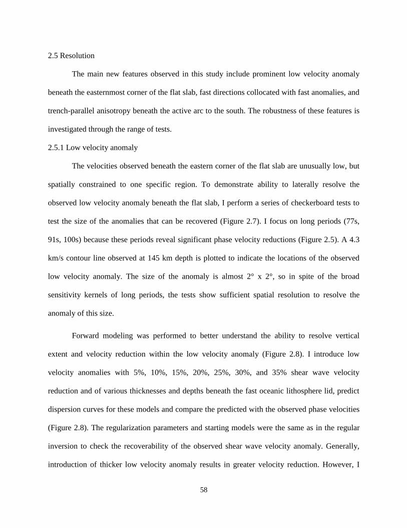
58
2.5 Resolution
The main new features observed in this study include prominent low velocity anomaly
beneath the easternmost corner of the flat slab, fast directions collocated with fast anomalies, and
trench-parallel anisotropy beneath the active arc to the south. The robustness of these features is
investigated through the range of tests.
2.5.1 Low velocity anomaly
The velocities observed beneath the eastern corner of the flat slab are unusually low, but
spatially constrained to one specific region. To demonstrate ability to laterally resolve the
observed low velocity anomaly beneath the flat slab, I perform a series of checkerboard tests to
test the size of the anomalies that can be recovered (Figure 2.7). I focus on long periods (77s,
91s, 100s) because these periods reveal significant phase velocity reductions (Figure 2.5). A 4.3
km/s contour line observed at 145 km depth is plotted to indicate the locations of the observed
low velocity anomaly. The size of the anomaly is almost 2° x 2°, so in spite of the broad
sensitivity kernels of long periods, the tests show sufficient spatial resolution to resolve the
anomaly of this size.
Forward modeling was performed to better understand the ability to resolve vertical
extent and velocity reduction within the low velocity anomaly (Figure 2.8). I introduce low
velocity anomalies with 5%, 10%, 15%, 20%, 25%, 30%, and 35% shear wave velocity
reduction and of various thicknesses and depths beneath the fast oceanic lithosphere lid, predict
dispersion curves for these models and compare the predicted with the observed phase velocities
(Figure 2.8). The regularization parameters and starting models were the same as in the regular
inversion to check the recoverability of the observed shear wave velocity anomaly. Generally,
introduction of thicker low velocity anomaly results in greater velocity reduction. However, I

59
was not able to match the observed phase velocity dispersion curves within error with any model
that incorporates a shear wave velocity anomaly of 5% regardless of the vertical extent or depth
of the anomaly. The models that do fit the observations within the confidence limits incorporate
low velocities ranging from ~75 km thick anomalies with 10% velocity reduction to ~10 km
thick anomalies with 35% velocity reduction. This test also shows that the actual low velocities
within the observed shear wave velocity anomaly are probably underestimated.

60
Figure 2.7 Checkerboard tests estimated from resolution matrix for 77, 91 and 100s. Colors
represent the recovered anomaly (see scale). Contour line of 4.3 km/s at 145 km (Figure 2.3c) is
shown to denote the observed low velocity anomaly. Dots are stations used in the study.

61
Figure 2.8 Recovery tests for the low velocity anomaly beneath the flat slab. a) Observed
dispersion curve (purple triangles) with error bars representing one standard deviation of
uncertainty. Blue dots represent the dispersion curve that corresponds to starting model shown
with blue line at c) (see text for details). Red circles show the best fit to the observed dispersion
curve yielding 1D shear wave velocity model shown with red line at c). b) Suit of starting
models with introduced low velocity anomaly with velocity reduction ranging from 10% to 35%
for which predicted dispersion curves fit the observations within the confidence limits. c)
Recovered models (black and gray lines) using predicted dispersion curves from 1D shear wave
velocity models shown at b) and our regular starting model (blue line). Red line represents the
model obtained using the observed dispersion curve.

62
2.5.2 Rayleigh wave azimuthal anisotropy
The resolution matrix diagonal for anisotropic terms is shown on Figure 2.9, Figure 2.10
and Figure 2.11. The Western and Eastern Cordillera are the best-resolved areas, while the
resolution decreases towards the coast, Sub-Andes, and Foreland. The resolution also varies
along the strike, being the highest just south of the subducting Nazca Ridge and between the
ridge and dense northern line of seismic stations.
A variety of tests were performed to check the robustness of the results for Rayleigh
wave phase anisotropy, including the sensitivity of the results to different a-priori starting models
and different damping parameters. The sensitivity of results to the anisotropic characteristics of
the starting model is tested by using three different starting models: one with no anisotropy, one
with uniform anisotropy of 2% strength with a N-S fast direction, and one with uniform
anisotropy of 2% strength with an E-W fast direction (Figure 2.9, Figure 2.10 and Figure 2.11).
These tests demonstrate the ability of the observations to constrain the patterns of fast directions,
regardless of the starting model used. For example, north of the projected subducted Nazca
Ridge, a consistent trench-parallel alignment of fast directions at shorter periods can be observed
near the coast and along Western Cordillera. At intermediate periods this pattern shifts inland
and persists at long periods along the Eastern Cordillera, while areas near the coast appear to
have roughly trench-perpendicular oriented fast directions. Also robust are the N-S to NNE-SSW
oriented fast directions at intermediate periods along the flat slab segment. The N-S to NNE-
SSW oriented fast directions along the ~71°W longitude at long periods (91s, 100s) persist
regardless of the starting model (Figure 2.9, Figure 2.10). Finally, to the south, trench-parallel
orientations of fast directions consistently appear at short periods (40-50 s) below the active
volcanic arc where the slab subducts steeply (Figure 2.6, Suppl. figure 7).

63
Tests using different damping parameters show that changing regularization parameters
affects the anisotropic magnitude, but not the orientation of fast directions (Figure 2.12). In
general, decreasing damping predictably increases magnitude. However, in well-resolved
regions, a maximum magnitude is attained, regardless of further damping decrease. I use the
highest damping (lowest covariance) that produces this maximum magnitude (covariance of
0.05) (Figure 2.12).

64
Figure 2.9 Resolution matrix diagonal for anisotropic terms and sensitivity test to different
starting models for 40, 66 and 91 s. The resolution represents the sum of the diagonal values of
the R-matrix for the two anisotropy terms at each grid node. Black bars represent the fast
directions scaled according to magnitude. First row shows sensitivity to model with no a-priori
anisotropy, middle row to model with uniform anisotropy of 2% strength with a E-W fast
direction, and the third row to model with uniform anisotropy of 2% strength with a N-S fast
direction. Background colors refer to resolution matrix diagonal. Red triangles are Holocene
volcanoes. Black rectangles, circles and stars are stations used in the study.
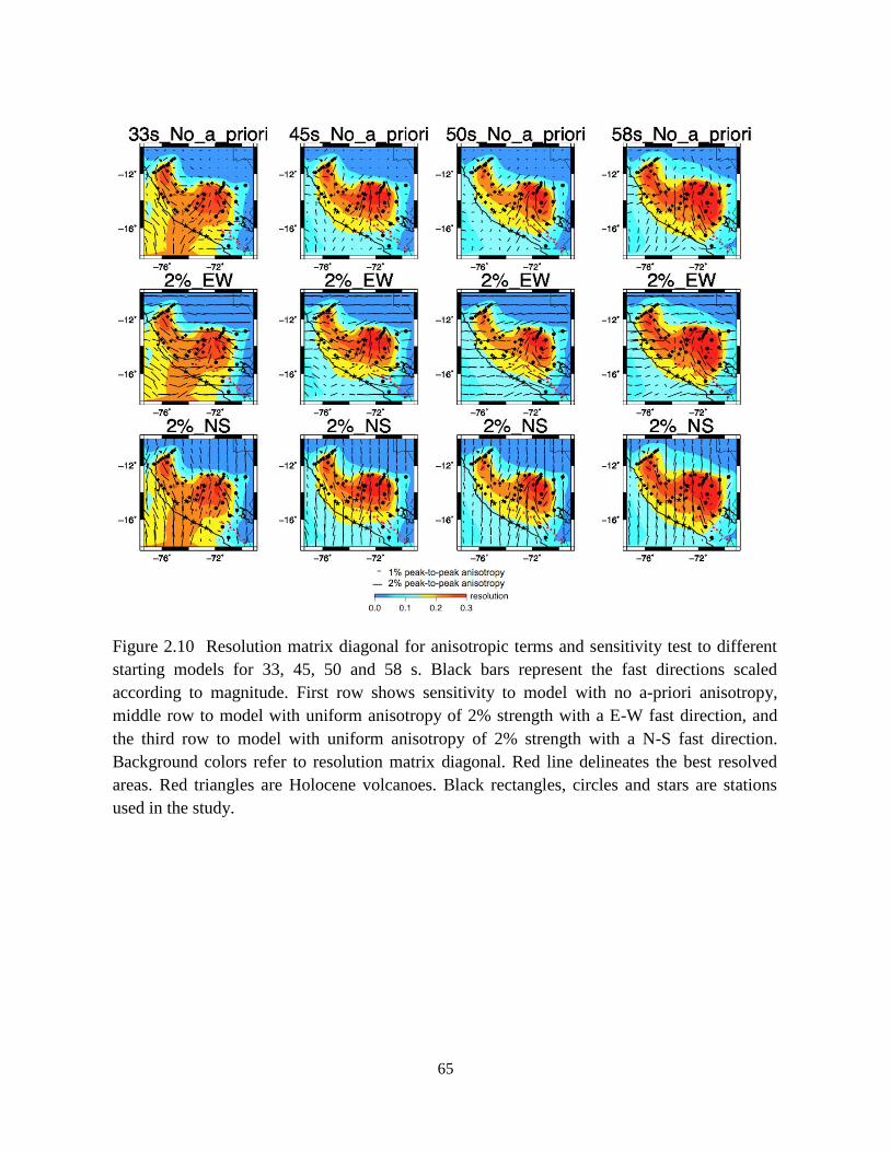
65
Figure 2.10 Resolution matrix diagonal for anisotropic terms and sensitivity test to different
starting models for 33, 45, 50 and 58 s. Black bars represent the fast directions scaled
according to magnitude. First row shows sensitivity to model with no a-priori anisotropy,
middle row to model with uniform anisotropy of 2% strength with a E-W fast direction, and
the third row to model with uniform anisotropy of 2% strength with a N-S fast direction.
Background colors refer to resolution matrix diagonal. Red line delineates the best resolved
areas. Red triangles are Holocene volcanoes. Black rectangles, circles and stars are stations
used in the study.

66
Figure 2.11 Resolution matrix diagonal for anisotropic terms and sensitivity test to different
starting models for 77, 100, 111 and 125 s. Black bars represent the fast directions scaled
according to magnitude. First row shows sensitivity to model with no a-priori anisotropy,
middle row to model with uniform anisotropy of 2% strength with a E-W fast direction, and the
third row to model with uniform anisotropy of 2% strength with a N-S fast direction.
Background colors refer to resolution matrix diagonal. Red line delineates the best resolved
areas. Red triangles are Holocene volcanoes. Black rectangles, circles and stars are stations
used in the study.

67
Figure 2.12 Tests for different damping values for period of 66s. Black bars represent the fast
directions scaled according to magnitude. Background colors refer to resolution matrix diagonal.
Red line delineates the best resolved areas. Red triangles are Holocene volcanoes. Black
rectangles, circles and stars are stations used in the study.
68
2.6 Discussion
2.6.1 Trench-parallel anisotropy beneath the active volcanic arc
The along-strike variations in slab geometry in southern Peru are accompanied by
substantial changes in observed anisotropy. Trench-parallel alignment of fast directions at short
periods appears at the southern end of the study area, where the Nazca plate subducts at a normal
dip angle, (40-50s, dashed orange area in Figure 2.5a,b and Figure 2.6b). The appearance of the
trench-parallel anisotropy at shorter periods constrains the anisotropic layer to lie either within or
above the slab. Trench-parallel alignment of fast directions in the mantle wedge above the
subducting slab has been observed or inferred in other subduction zones, including in Costa Rica
and Nicaragua [Hoernle et al., 2008], the Aleutians [Mehl et al., 2003], the Mariana subduction
system [Pozgay et al., 2007], and in the Japanese Ryukyu arc [Long and Hilst, 2006]. These
observations can be reconciled with viscous coupling between the downgoing plate and the
overlying mantle wedge material, causing two-dimensional corner flow in the mantle wedge [e.g.
Fischer et al., 2000], if the presence of B-type olivine fabric is invoked. B-type fabric tends to
align fast axes perpendicular to the flow direction [Jung and Karato, 2001], and requires the
presence of low temperatures, high stresses, and some amount of water [Kneller et al., 2005].
The seismicity along the steeply dipping slab in southern Peru is abundant [e.g. Kumar et al,
2016], suggesting the release of fluids into the wedge via metamorphic dehydration reactions
[e.g., Kirby et al., 1996]. However, high heat flow [Hamza et al., 2005] and the presence of an
active volcanic arc above the steeply dipping slab suggest elevated temperature and low stresses,
and thus conditions less favorable for the occurrence of B type olivine.
Another possibility is arc parallel flow in the mantle wedge that can be caused by some
combination of trench retreat and variations in slab dip [Hoernle et al., 2008; Kneller and van

69
Keken, 2008]. According to this scenario the A-, C-, D- or E- type olivine crystals tend to align
the fast symmetry axis (a axis) in the warm mantle wedge roughly parallel to the flow. The
ambient conditions in the mantle wedge beneath the active volcanic arc with elevated
temperatures and high water content are favorable for the occurrence of C-type olivine [Karato,
2008], which would be the best candidate to explain the observed pattern.
A third possibility involves serpentine deformation within the hydrated mantle wedge
[Katayama et al., 2009]. The serpentine tends to align the slow c-axis orthogonally to the shear
plane during the deformation. As mentioned earlier, the abundant seismicity might indicate
dehydration of the slab and hydration of the mantle wedge. In addition, the low shear velocities
that can be observed above the steeply descending plate and beneath the active volcanic arc
(Figure 2.3, transect CC’) likely relate to combination of high temperatures and presence of
fluids.
A fourth possibility relates to fault-induced seismic anisotropy along the trench-parallel
trending outer rise faults created by bending of the slab before entering the trench [Faccenda et
al., 2008]. In this case the anisotropy is caused by crystallographic and shape-preferred
orientation of hydrated fault surfaces [Faccenda et al., 2008] possibly in combination with
dehydration and increased pore pressure in these fault zones during subduction [Healy et al.,
2009]. Substantial shear wave velocity reduction along the upper part of the subducting plate
and/or along the interface between two plates in southern Peru has been recently imaged by Kim
and Clayton [2015]. The velocity reduction was interpreted as slab hydration of outer rise faults
and subsequent dehydration upon subduction, consistent with this and previous scenarios.
It is hard to discriminate between the last three scenarios, particularly since the sensitivity
of surface waves at the relevant periods do not allow me to distinguish between anisotropy

70
within the wedge and the shallow part of the subducting slab. Future comparison of these results
with shear wave splitting may help to better understand the cause of the trench-parallel
anisotropy to the south.
2.6.2 Evidence for flow through the slab tear
The slab geometry north of the subducting Nazca Ridge is very complex: the slab is torn
to the west, while the flat slab remnants still persist to the east (Figure 2.3d) [Antonijevic et al.,
2015]. The slab tear probably continues up to ~350 km depth [Scire et al., 2016].
One possible explanation for the trench parallel fast directions that are aligned with the
trench parallel low velocity anomaly north of the Nazca Ridge is that this low velocity material
represents asthenosphere flowing through the inferred tear in the Nazca Plate (Figure 2.13,
anomaly “MF”). By comparing fast directions of long and intermediate periods I notice gradual
westward progression of the trench-parallel pattern as the periods get shorter (Figure 2.13
d,c,b,a). This might suggest that the sub-slab mantle flow gets shallower from east to west,
consistent with the asthenosphere flowing above the normally dipping slab to the west (anomaly
“S” in Figure 2.13) and below the flat slab remnants to the east (anomaly “FSR” in Figure 2.13
a,b). The direction of this flow is not well constrained. It could either be flowing from the mantle
wedge above the normally dipping slab west of the tear to the sub-slab mantle beneath the flat
slab or the other way around.
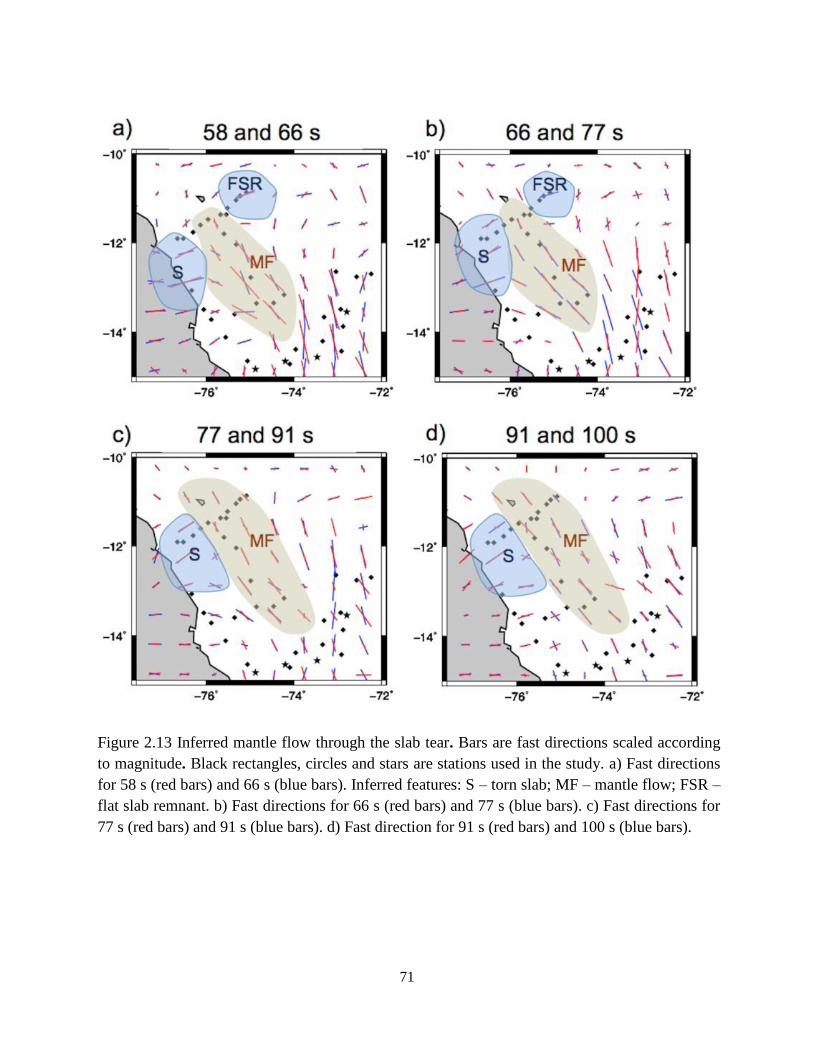
71
Figure 2.13 Inferred mantle flow through the slab tear. Bars are fast directions scaled according
to magnitude. Black rectangles, circles and stars are stations used in the study. a) Fast directions
for 58 s (red bars) and 66 s (blue bars). Inferred features: S – torn slab; MF – mantle flow; FSR –
flat slab remnant. b) Fast directions for 66 s (red bars) and 77 s (blue bars). c) Fast directions for
77 s (red bars) and 91 s (blue bars). d) Fast direction for 91 s (red bars) and 100 s (blue bars).

72
2.6.3 Low velocity anomaly beneath the easternmost corner of the flat slab
Probably the most striking feature south of the inferred tear is a pervasive low velocity
anomaly at sub-slab depths beneath the inboard easternmost corner of the flat slab. As described
earlier, instead of slab-related high velocities I observe modest low velocities all along the plate
below the subducted Nazca Ridge that becomes even further reduced ~250 km away from the
trench (Figure 2.3c and 2.3e, Figure 2.4).
Several factors could cause the absence of slab-related high velocities along the ridge
upon subduction. First, resolution is poor west of the stations between the trench and the
horizontal portion of the slab. This is because of a lack of stations offshore, and because stations
along the coast are usually nosier, meaning fewer useable data were obtained from these
locations. Therefore, at least for areas west of the array, the lack of high velocities could simply
be an artifact of undersampling. Second, the crust of the subducting Nazca Ridge is very thick
(~18 km) [Hampel et al., 2004] and possibly hydrated [Kim and Clayton, 2015]. The hydrated,
over-thickened crust and upper sedimentary layers will have low shear wave velocities, which
could vertically smear into the oceanic mantle lithosphere in my model, making the expected
oceanic-lithosphere-related high velocities more difficult to resolve. Third, inherited mantle
structures from the formation of the Nazca Ridge may result in persistent lower velocities in the
associated mantle lithosphere. In general, asthenospheric flow in the form of small-scale
convection and/or viscous fingering instabilities have been invoked to explain the formation of
intraplate ridges and seamounts [Weereratne et al., 2007] and accompanied delayed
cooling/thickening of the oceanic lithosphere [Davaille and Lees, 2004]. Recently, Forsyth and
Weereratne (2014) found high attenuation and low shear wave velocities beneath the Shatsky
Rise in the northwestern Pacific. This area hasn’t been affected by volcanism within the past
73
~150 Ma, which suggests that low velocity anomalies beneath intraplate volcanic features can
persist for long periods of time. Woods et al. [1994] estimated a substantial reduction in shear
wave velocity (below 4 km/s) under the Nazca Ridge in the eastern Pacific Ocean basin using
Rayleigh waveforms that propagate along entire length of the ridge. This velocity reduction may
indicate the presence of small melt pockets beneath the ridge to the west. In addition, among
samples of volcanic rocks obtained from the Nazca Ridge, a few were approximately 5 - 13 Ma
younger, showing evidence of a rejuvenation of Nazca Ridge volcanism [Ray et al., 2012]. The
velocities along the first ~250 km of subducted ridge are not exceptionally low (Figure 2.3e).
This indicates either that partial melt does not exist beneath the ridge any longer, or that partial
melt regions are very small and localized. Furthermore, the intraplate volcanism could have
delayed the usual cooling and thickening of oceanic lithosphere or even thermally ablated the
existing mantle lithosphere. Thinned oceanic mantle lithosphere along the ridge in combination
with vertically smeared low velocities from over-thickened crust and limited resolution along the
coastal region could produce the observed modest lower slab-related shear wave velocities at
first ~250 km of subducted ridge.
While inherited structures and resolution can provide an explanation for the moderately
low velocities observed to the west, they do not explain the sharp decrease in velocity observed
beneath the easternmost corner of the flat slab. The anomaly is within the seismic array and is
well resolved (Figure 2.7). Any inherited structure that might be invoked to explain velocities
further to the west would likely remain constant along the extent of the subducted Nazca Ridge.
The abrupt additional decrease in velocities beneath the slab in this region requires additional
explanation.

74
Several factors could contribute to the strengthening of the low velocity anomaly beneath
the easternmost corner of the flat slab. These include increases in temperature, the presence of
volatiles, and the presence of partial melting. Only minimum amounts of change can be
calculated based on the observed decrease in velocity due to likely underestimation of the actual
low velocity anomalies caused by damping of the inversion [see forward modeling in Figure 2.8
and Figure S2.3]. In the absence of melting or volatiles, the difference in shear velocities from
west to east would require an additional increase in temperature of at least ~200°C [Cammarano
et al., 2003]. The presence of water would also reduce velocities, even in the absence of partial
melting or temperature change. The effect of high water content is similar to that of increased
temperature, with 0.15 wt% of water in olivine roughly corresponding to an increase in
temperature for 200°C [Karato, 2003]. A combination of temperature and/or volatiles could
promote melting which in turn would also have a pronounced effect on seismic velocities [Katz
et al., 2003]. To recover the observed velocities presence of at least 1% partial melting (7.9%
velocity deviation [Hammond and Humphreys, 2000]) over a 70-90 km thick vertical column or
2% partial melting (22% velocity deviation) within a 25-35 km thick vertical column is required
(see forward modeling in Figure S2.3) .
There are a number of possible scenarios that could lead to some combination of changes
in temperature, volatiles, or partial melting beneath the easternmost corner of the flat slab.
Because this feature is unlikely to be caused only by an inherited structure, some degree of
mantle flow must be involved in its formation. Roughly speaking, the sub-slab mantle in this
region could flow trench parallel (either south to north or north to south), vertically, or both.
Depending on the flow directions, different combinations of temperature, melting, and volatile
presence emerge as contributing factors to this low velocity anomaly.

75
In the absence of any vertical motion, mantle flow directed south to north (as suggested
previously by Russo and Silver [1994]) should not produce radically different velocities along
strike, and is therefore difficult to reconcile with my observations. Vertical (upward directed)
mantle flow, however, could explain the observations by introducing warmer material to the area
directly beneath the inboard corner of the flat slab. A vertical component to mantle flow would
be consistent with the observed nulls from SKS, sSKS, and PKS shear wave splitting beneath
this portion of flat slab [Eakin 2015]. The low velocity anomaly is reduced laterally with depth
and confines to the inboard easternmost corner beneath the flat slab (Figure 2.3, Figure 2.4). This
suggests that any vertical flow and possible associated decompression partial melting is localized
both laterally and in depth. Future examination of radial anisotropy (Rayleigh vs. Love waves) is
necessary to confirm the presence of such vertical flow.
Another possibility is the presence of water and possible associated flux melting.
Normally, regional sub-slab low velocities are not attributed to increases in volatiles due to the
absence of an obvious source of significant amounts of water. However, the inferred tear in the
subducted plate to the north [Antonijevic et al., 2015] offers this additional intriguing possibility.
If flow beneath this portion of the Nazca plate trends trench parallel from north to south instead
south to north, the mantle from above the torn slab could be hydrated by that slab and then flow
south, ending up below the flat slab. In this case, the observed trench-parallel alignment of fast
directions north of the projected Nazca Ridge would correspond to the N-S directed flow.
Eventually, this hydrated material might collect in the inboard corner of the contorted underside
of the flat slab resulting in volatile-rich sub-slab mantle and/or flux melting (Figure 2.14). Given
that the tear occurred recently [Antonijevic et al., 2015], this scenario is possible only if the
volatile-rich sub-slab mantle had enough time to reach the edge of the flat slab region.

76
Both an increase in temperature/decompression melting and the presence of volatiles/flux
melting can equally well explain the velocity reduction beneath the easternmost corner of the flat
slab, so discriminating between the two is difficult. In either case, however, the observed
anomaly might have important geodynamic implications since the material beneath this corner is
presumably more buoyant than the surrounding mantle and/or could thermally ablate the slab
from beneath. Recent high resolution imaging of the southernmost part of the flat slab reveals an
inboard upward motion of the flat slab roughly beneath the Western/Eastern Cordillera boundary
[Ma and Clayton, 2015]. This unusual slab geometry has been attributed to interplate suction.
However, the location of the flat slab’s inferred upward deflection spatially coincides with this
prominent low velocity anomaly beneath the slab. The thermally ablated/thinned oceanic mantle
lithosphere of the subducting ridge and/or presence of volatiles/partial melting below this corner
could contribute to overall slab buoyancy, providing additional support to this upward motion.
Future geodynamical modeling is necessary to better understand the effects of this anomaly to
complex slab geometry in this corner.

77
Figure 2.14 Schematic representation of the slab fabric and mantle flow through the tear. a)
Reference figure from 1.23d with the inferred features. b) The top of the slab is inferred from
earthquake distribution [Antonijevic et al., 2015]; lateral and vertical extent of the low velocity
anomaly is inferred from the 3D shear wave velocity model. The black arrow denotes relative
motion of the Nazca Plate [Gripp and Gordon, 2002]. Green marked area refers to subducting
Nazca Ridge. Blue arrows show slab fabric. Red arrows refer to mantle flow through the tear
north of the ridge. If the mantle flows from south to north, it may carry hydrous phases released
from the torn slab.
78
2.6.4 Slab-related anisotropy
Some of the observed anisotropy is associated with the fast velocity anomalies of the
subducted Nazca Plate. Before being subducted oceanic plates usually preserve primary
(fossilized) fabric dating from early slab formation along the mid-oceanic ridge. The direction of
azimuthal anisotropy in young oceanic plates is typically related to A-type olivine within the
oceanic lithospheric mantle, which tend to align fast axes along the spreading direction [e.g.
Hess, 1964]. Even though this fossil fabric has been generally more successfully observed in
younger oceanic plates, recent studies show that it can persist in older slabs, too. For example,
using Rayleigh wave phase anisotropy, Smith et al., [2004] found evidence of stratification in
azimuthal anisotropy with depth across the Pacific. They found that the fast directions in the
upper lithosphere (<100km) correlate well with paleo-spreading directions, reflecting fossilized
azimuthal anisotropy, while greater depths illuminate current ambient flow direction. This
primary (fossilized) fabric can persist upon entering the subduction zone [Audet 2013] or can be
modified upon subduction. The serpentinization along the outer-rise faults in the upper part of
the slab [Faccenda et al., 2008], or, alternatively, substantial deformation within the slab due to
rapid change in slab geometry [Eakin et al., 2016] can lead to alteration of the slab’s primary
fabric.
Recently, Eakin et al. [2016] demonstrated that the fossil slab fabric in the 200-400 km
depth range in southern Peru is overprinted due to the substantial along-strike extension that slab
undergoes while changing its geometry from flat to steep. According to their model, the CPO of
olivine in this specific area rotates to become sub-parallel to the slab depth contours during
deformation. My observations along the southern margin of the flat slab are consistent with this
model and extend that interpretation to shallower depths. I observe a rotation of fast axes from
79
trench-perpendicular to N-S/NNW-SSE at intermediate periods (58, 66 s), that correspond to the
depth of the subducting plate (Figure 2.1, Figure 2.3 and Figure 2.4). This anisotropic pattern is
also aligned with fast velocities (dashed blue area in Figure 2.5c,d,e) consistent with my
interpretation of slab-related anisotropy. I observe the strongest anisotropy along the southern
edge of the flat slab, where the slab is heavily contorted due to a rapid change in slab geometry
from flat to steep [Ma and Clayton, 2014; Phillips and Clayton, 2012]. The orientation of fast
axes along the southernmost edge of the flat slab/transition zone at intermediate periods (58, 66s,
Figure 2.5c,d) is consistent with the orientation of T axes (the maximum extension direction)
inferred from focal mechanism solutions [Kumar et al., 2016]. The pattern shifts inland at longer
periods (Figure 2.5e,f, Figure 2.6c,d), which suggests that modified slab fabric persists at greater
depths.
My observations are consistent with Eakin et al. [2016] along the southern margin of the
flat slab. In areas north of the ridge, where the slab is torn and has resumed normal subduction
[Antonijevic et al., 2015], I find different patterns of slab-related anisotropy. Roughly trench-
perpendicular fast directions at intermediate and longer periods align with a seismically fast
anomaly (dashed green area in Figure 2.5c,d,e,f), which I interpret as the anisotropic pattern
coming from the slab the west of the tear. This slab is not affected by flat-slab related
deformation, and therefore preserves its paleo-fabric. The contrast in the observed anisotropic
patterns to the south and north illuminates differences in strain that the Nazca plate undergoes
along the strike. The extension within the contorted slab to the south has led to alternation of the
preexisting slab fabric, while the preservation of the fossil slab fabric to the north indicates that
the slab here has not undergone the same deformation (Figure 2.14). This is additional evidence
80
showing that the previously assumed extensive Peruvian flat slab is not uniformly flat along the
strike.
2.7 Conclusion
Observations of anisotropic Rayleigh wave phase velocities indicate that the complex
slab geometry in southern Peru affects the surrounding mantle flow field. To the south, where the
slab subducts steeply, the observed trench-parallel oriented fast directions beneath the active
volcanic arc may relate either to the mantle wedge and/or subducting plate. To the north, a
pronounced low velocity anomaly appears beneath the easternmost corner of the flat slab. The
anomaly may be produced either by increased temperature and/or decompression melting due to
small-scale vertical flow beneath this corner, or by the presence of volatiles and/or flux melting
that could be caused by southward directed, volatile-rich sub-slab mantle flow. Future
examination of radial anisotropy should be able to verify the existence of vertical flow beneath
this corner. In either case, the sub-slab material beneath this corner is presumably more buoyant
than the surrounding mantle and may provide an additional dynamic contribution to the inferred
upward deflection of the flat slab in this region.
These results indicate that the mantle flow above the torn slab north of the subducted
Nazca Ridge continues beneath the flat slab segment. The slab tear created a new pathway that
connects two mantle reservoirs. However, the directions of this flow is poorly constrained, since
azimuthal anisotropy can reveal the orientation, but not the direction of mantle flow.
Based on slab-related anisotropy I find that the slab’s internal deformation substantially
varies along the strike. South of the subducting Nazca Ridge the extension within excessively
contorted slab alters the slab fabric. These results indicate that this altered slab fabric persists at

81
greater depths. In contrast, the slab tear to the north reduces the strain within the torn slab
allowing the slab’s primary (fossilized) fabrics to stay preserved upon subduction.

82
REFERENCES
1. Anderson, M. L., Zandt, G., Triep, E., Fouch, M., & Beck, S. (2004). Anisotropy and mantle
flow in the Chile‐Argentina subduction zone from shear wave splitting analysis. Geophysical
Research Letters, 31(23). doi:10.1029/2004GL020906
2. Antonijevic, S. K., Wagner, L. S., Kumar, A., Beck, S. L., Long, M. D., Zandt, G.,Tavera, H.
& Condori, C. (2015). The role of ridges in the formation and longevity of flat slabs. Nature,
524(7564), 212-215. doi:10.1038/nature14648
3. Audet, P. (2013). Seismic anisotropy of subducting oceanic uppermost mantle from fossil
spreading. Geophysical Research Letters, 40(1), 173-177. doi: 10.1029/2012GL054328
4. Cahill, T., & Isacks, B. L. (1992). Seismicity and shape of the subducted Nazca plate.
Journal of Geophysical Research: Solid Earth (1978–2012), 97(B12), 17503-17529. doi:
10.1029/92JB00493
5. Cammarano, F., Goes, S., Vacher, P., & Giardini, D. (2003). Inferring upper-mantle
temperatures from seismic velocities. Physics of the Earth and Planetary Interiors, 138(3),
197-222.doi: 10.1016/S0031-9201(03)00156-0
6. Couch, R. and Whitsett, R.M., 1981. Structure of the Nazca Ridge and the continental shelf
and slope of southern Peru. Geol. Soc. Am. Mem., 154: 569-586. doi: 10.1130/MEM154-
p569
7. Davaille, A., & Lees, J. M. (2004). Thermal modeling of subducted plates: tear and hotspot at
the Kamchatka corner. Earth planet. Sci. Lett., 226(3), 293-304.
doi:10.1016/j.epsl.2004.07.024
8. DeMets, C., Gordon, R. G., & Argus, D. F. (2010). Geologically current plate motions.
Geophysical Journal International, 181(1), 1-80. doi: 10.1111/j.1365-246X.2009.04491.x
9. Di Leo, J. F., Walker, A. M., Li, Z. H., Wookey, J., Ribe, N. M., Kendall, J. M., & Tommasi,
A. (2014). Development of texture and seismic anisotropy during the onset of subduction.
Geochemistry, Geophysics, Geosystems, 15(1), 192-212. doi:10.1002/2013GC005032
10. Dougherty, S. L., & Clayton, R. W. (2014). Seismic structure in southern Peru: evidence for
a smooth contortion between flat and normal subduction of the Nazca Plate. Geophysical
Journal International, 200(1), 534-555. http://dx.doi.org/10.1093/gji/ggu415
11. Eakin, C. M., & Long, M. D. Complex anisotropy beneath the Peruvian flat slab from
frequency‐dependent, multiple‐phase shear wave splitting analysis. J. Geophys. Res.: Solid
Earth. 118(9), 4794-4813 (2013). doi: 10.1002/jgrb.50349
12. Eakin, C. M., Long, M. D., Beck, S. L., Wagner, L.S., Tavera, H. & Condori, C. (2014).
Response of the mantle to flat slab evolution: Insights from local S splitting beneath Peru. J.
Geophys. Res. 41(10), 3438-3446 (2014). doi: 10.1002/2014GL059943

83
13. Eakin, C. M., Long, M. D., Beck, S. L., Wagner, L.S., Tavera, H. & Condori, C. Upper
mantle anisotropy beneath Peru from SKS splitting: Constraints on flat slab dynamics and
interaction with the Nazca Ridge. Earth planet. Sci. Lett., 412 (2015): 152-162.
doi:10.1016/j.epsl.2014.12.015
14. Eakin, C. M., Long, M. D., Scire, A., Beck, S. L., Wagner, L. S., Zandt, G., & Tavera, H.
(2016). Internal deformation of the subducted Nazca slab inferred from seismic anisotropy.
Nature Geoscience, 9(1), 56-59. doi: 10.1038/ngeo2592.
15. Faccenda, M., L. Burlini, T. V. Gerya, and D. Mainprice (2008), Fault-induced anisotropy by
hydration in subducting oceanic plates, Nature, 455, 1097–1101. doi:10.1038/nature07376
16. Faccenda, M., & Capitanio, F. A. (2013). Seismic anisotropy around subduction zones:
Insights from three‐dimensional modeling of upper mantle deformation and SKS splitting
calculations. Geochemistry, Geophysics, Geosystems, 14(1), 243-262.
doi:10.1002/ggge.20055
17. Fischer, K.M., Parmentier, E.M., Stine, A.R.,Wolf, E.R., 2000. Modeling anisotropy and
plate-driven flow in the Tonga subduction zone back arc. J. Geophys. Res. 105, 16,181–
16,191. doi: 10.1029/1999JB900441
18. Forsyth, D. W., & Li, A. (2005). Array analysis of two‐dimensional variations in surface
wave phase velocity and azimuthal anisotropy in the presence of multipathing interference.
Seismic Earth: Array Analysis of Broadband Seismograms, 81-97. doi: 10.1029/157GM06
19. Forsyth,D.W. & Weereratne, D. (2014). Attenuation in the Upper Mantle beneath “Normal”
Old Seafloor in the Western Pacific. DI44A-06. AGU Fall Meeting 2014, San Francisco,
California.
20. Gripp, A. E., & Gordon, R. G. (2002). Young tracks of hotspots and current plate velocities.
Geophysical Journal International, 150(2), 321-361. doi: 10.1046/j.1365-
246X.2002.01627.x
21. Gutscher, M. A., Spakman, W., Bijwaard, H., & Engdahl, E. R. (2000a). Geodynamics of flat
subduction: seismicity and tomographic constraints from the Andean margin. Tectonics,
19(5), 814-833. doi: 10.1029/1999TC001152
22. Hammond, W. C., & Humphreys, E. D. (2000). Upper mantle seismic wave velocity- Effects
of realistic partial melt geometries. Journal of Geophysical Research, 105(10), 975-10. doi:
10.1029/2000JB900041
23. Hampel, A., Kukowski, N., Bialas, J., Huebscher, C., & Heinbockel, R. Ridge subduction at
an erosive margin: The collision zone of the Nazca Ridge in southern Peru. J. Geophys. Res:
Solid Earth. 109(B2) (2004). doi: 10.1029/2003JB002593
24. Hampel, A. (2002). The migration history of the Nazca Ridge along the Peruvian active
margin: A re-evaluation. Earth planet. Sci. Lett.,, 203(2), 665-679. doi: 10.1016/S0012-
821X(02)00859-2

84
25. Hamza, V. M., Dias, F. J. S., Gomes, A. J., & Terceros, Z. G. D. (2005). Numerical and
functional representations of regional heat flow in South America. Physics of the Earth and
Planetary Interiors, 152(4), 223-256. doi: 10.1016/j.pepi.2005.04.009
26. Healy, D., Reddy, S. M., Timms, N. E., Gray, E. M., & Brovarone, A. V. (2009). Trench-
parallel fast axes of seismic anisotropy due to fluid-filled cracks in subducting slabs. Earth
planet. Sci. Lett., 283(1), 75-86. doi: 10.1016/j.epsl.2009.03.037
27. Hess, H. H. (1964). Seismic anisotropy of the uppermost mantle under oceans. Nature 203,
629 - 631 (08 August 1964); doi:10.1038/203629a0.
28. Hoernle, K., Abt, D. L., Fischer, K. M., Nichols, H., Hauff, F., Abers, G. A., van den
Bogaard, P., Heydolph, K., Alvarado, G., Protti, M. and Strauch, W. (2008). Arc-parallel
flow in the mantle wedge beneath Costa Rica and Nicaragua. Nature, 451(7182), 1094-1097.
doi: 10.1038/nature06550
29. Instituto Geológico Minero y Metalúrgico – INGEMMET, On-line Catalog, accessed at
http://www.ingemmet.gob.pe, Peru (2014).
30. Jaillard, E., Hérail, G., Monfret, T., Díaz-Martínez, E., Baby, P., Lavenu, A., & Dumont, J. F.
(2000). Tectonic evolution of the Andes of Ecuador, Peru, Bolivia and northernmost Chile.
Tectonic Evolution of South America, 31, 481-559.
31. James, D. E. (1971). Andean crustal and upper mantle structure. Journal of Geophysical
Research, 76(14), 3246-3271. doi: 10.1029/JB076i014p03246
32. Jung, H., Karato, S.-i., 2001. Water-induced fabric transitions in olivine. Science 293, 1460–
1463. doi: 10.1126/science.1062235
33. Karato, S. I. (2003). Mapping water content in upper mantle. Geophysical L Monograph-
American Geophysical Union, 138, 135-152. doi: 10.1029/138GM08
34. Karato, S. I., Jung, H., Katayama, I., & Skemer, P. (2008). Geodynamic significance of
seismic anisotropy of the upper mantle: new insights from laboratory studies. Ann. Rev.
Earth Planet. Sci., 36, 59-95. doi: 10.1146/annurev.earth.36.031207.124120
35. Katayama, I., Hirauchi, K. I., Michibayashi, K., & Ando, J. I. (2009). Trench-parallel
anisotropy produced by serpentine deformation in the hydrated mantle wedge. Nature,
461(7267), 1114-1117. doi: 10.1038/nature08513
36. Katz, R. F., Spiegelman, M., & Langmuir, C. H. (2003). A new parameterization of hydrous
mantle melting. Geochemistry, Geophysics, Geosystems, 4(9). doi: 10.1029/2002GC000433
37. Kennett, B. L. N. IASPEI 1991 Seismological Tables (Bibliotech, Canberra, Australia,
1991).

85
38. Kim, Y., & Clayton, R. W. (2015). Seismic properties of the Nazca oceanic crust in southern
Peruvian subduction system. Earth planet. Sci. Lett., 429, 110-121.
http://dx.doi.org/10.1016/j.epsl.2015.07.055
39. Kirby, S., Engdahl, R. E., & Denlinger, R. (1996). Intermediate‐depth intraslab earthquakes
and arc volcanism as physical expressions of crustal and uppermost mantle metamorphism in
subducting slabs. Subduction top to bottom, 195-214. doi: 10.1029/GM096p0195
40. Kneller, E.A., van Keken, P.E., Karato, S.-i., Park, J., 2005. B-type olivine fabric in the
mantle wedge: Insights from high-resolution non-Newtonian subduction zone models. Earth
planet. Sci. Lett.237, 781–797. doi: 10.1029/2001DC000256
41. Kneller, E. A., & Van Keken, P. E. (2008). Effect of three‐dimensional slab geometry on
deformation in the mantle wedge: Implications for shear wave anisotropy. Geochemistry,
Geophysics, Geosystems, 9(1). doi: 10.1029/2007GC001677
42. Kumar, A., Wagner, L. S., Beck, S. L., Long, M. D., Zandt, G., Young, B.,Tavera, H. and
Minaya, E. (2016). Seismicity and state of stress in the central and southern Peruvian flat
slab. Earth and Planetary Science Letters, 441, 71-80.
43. Long, M. D., & Becker, T. W. (2010). Mantle dynamics and seismic anisotropy. Earth
planet. Sci. Lett., 297(3), 341-354.doi:10.1016/j.epsl.2010.06.036
44. Long, M. D., & van der Hilst, R. D. (2006). Shear wave splitting from local events beneath
the Ryukyu arc: trench-parallel anisotropy in the mantle wedge. Physics of the earth and
planetary interiors, 155(3), 300-312. doi: 10.1016/j.pepi.2006.01.003
45. Ma, Y. & Clayton, R.W., 2014. The crust and uppermost mantle structure of Southern Peru
from ambient noise and earthquake surface wave analysis, Earth planet. Sci. Lett., 395, 61–
70.
46. Ma, Y., & Clayton, R. W. (2015). Flat slab deformation caused by interplate suction force.
Geophysical Research Letters., 42(17), 7064-7072. doi: 10.1002/2015GL065195
47. Macharé, J., & Ortlieb, L. (1992). Plio-Quaternary vertical motions and the subduction of the
Nazca Ridge, central coast of Peru. Tectonophysics, 205(1), 97-108. doi: 10.1016/0040-
1951(92)90420-B
48. Mehl, L., Hacker, B. R., Hirth, G., & Kelemen, P. B. (2003). Arc‐parallel flow within the
mantle wedge: Evidence from the accreted Talkeetna arc, south central Alaska. Journal of
Geophysical Research: Solid Earth (1978–2012), 108(B8). doi:10.1029/2002JB002233
49. Müller, R. D., Sdrolias, M., Gaina, C., & Roest, W. R. (2008). Age, spreading rates, and
spreading asymmetry of the world's ocean crust. Geochemistry, Geophysics, Geosystems,
9(4). doi: 10.1029/2007GC001743
86
50. Peyton, V., Levin, V., Park, J., Brandon, M., Lees, J., Gordeev, E., & Ozerov, A. (2001).
Mantle flow at a slab edge: Seismic anisotropy in the Kamchatka region. Geophys. Res. Lett,
28(2), 379-382. doi: 10.1029/2000GL012200
51. Phillips, K., Clayton, R. W., Davis, P., Tavera, H., Guy, R., Skinner, S. & Aguilar, V. (2012).
Structure of the subduction system in southern Peru from seismic array data. Journal of
Geophysical Research: Solid Earth (1978–2012), 117(B11). doi: 10.1029/2012JB009540
52. Phillips, K., & Clayton, R. W. Structure of the subduction transition region from seismic
array data in southern Peru. Geophys. J. Int. ggt504 (2014). doi: 10.1029/2012JB009540
53. Porritt, R. W., Becker, T. W., & Monsalve, G. (2014). Seismic anisotropy and slab dynamics
from SKS splitting recorded in Colombia. Geophysical Research Letters, 41(24), 8775-8783.
doi: 10.1002/2014GL061958
54. Pozgay, S. H., Wiens, D. A., Conder, J. A., Shiobara, H., & Sugioka, H. (2007). Complex
mantle flow in the Mariana subduction system: evidence from shear wave splitting.
Geophysical Journal International, 170(1), 371-386. doi: 10.1111/j.1365-
246X.2007.03433.x.
55. Ray, J.S., Mahoney, J.J.,Duncan, R.A., Ray, J.,Wessel, P.&Naar,D.F., 2012.Chronology and
geochemistry of lavas from the Nazca Ridge and Easter Seamount Chain: an ∼30 Myr
hotspot record, J. Petrol., 53, 1417–1448. doi: 10.1093/petrology/egs021
56. Rosenbaum, G., Giles, D., Saxon, M., Betts, P. G., Weinberg, R. F., & Duboz, C. Subduction
of the Nazca Ridge and the Inca Plateau: Insights into the formation of ore deposits in Peru.
Earth and Planet. Sci. Lett. 239(1), 18-32 (2005). doi: 10.1016/j.epsl.2005.08.003
57. Russo, R. M., & Silver, P. G. (1994). Trench-parallel flow beneath the Nazca plate from
seismic anisotropy. Science, 263(5150), 1105-1111. doi: 10.1126/science.263.5150.110
58. Saito, M. in Seismological Algorithms: Computational Methods and Computer Programs.
(ed. Doornbos, D. J.) 293–319 (Elsevier, 1988)
59. Scire, A., Zandt, G., Beck, S., Long, M., Wagner, L., Minaya, E., & Tavera, H. (2016).
Imaging the transition from flat to normal subduction: variations in the structure of the Nazca
slab and upper mantle under southern Peru and northwestern Bolivia. Geophysical Journal
International, 204(1), 457-479. doi: 10.1093/gji/ggv452
60. Skemer, P., & Hansen, L. N. (2015). Inferring upper-mantle flow from seismic anisotropy:
An experimental perspective. Tectonophysics. http://dx.doi.org/10.1016/j.tecto.2015.12.003
61. Skemer, P., Warren, J. M., & Hirth, G. (2012). The influence of deformation history on the
interpretation of seismic anisotropy. Geochemistry, Geophysics, Geosystems, 13(3).
doi:10.1029/2011GC003988

87
62. Smith, M. L., & Dahlen, F. A. (1973). The azimuthal dependence of Love and Rayleigh
wave propagation in a slightly anisotropic medium. Journal of Geophysical Research, 78(17),
3321-3333. doi: 10.1029/JB078i017p03321
63. Smith, D. B., Ritzwoller, M. H., & Shapiro, N. M. (2004). Stratification of anisotropy in the
Pacific upper mantle. Journal of Geophysical Research: Solid Earth (1978–2012), 109(B11).
doi: 10.1029/2004JB003200
64. Snoke, J. A., Sacks, I. S., & James, D. E. Subduction beneath western South America:
evidence from converted phases. Geophys. J. of the Royal Astronomical Soc., 59(1), 219-225
(1979). doi: 10.1111/j.1365-246X.1979.tb02562.x
65. Steinberger, B. (2002). Motion of the Easter hot spot relative to Hawaii and Louisville hot
spots. Geochemistry, Geophysics, Geosystems, 3(11), 1-27. doi: 10.1029/2002GC000334
66. Tassara, A., Go ̈tze, H.J., Schmidt, S. & Hackney, R., 2006. Three-dimensional density
model of the Nazca plate and the Andean continental margin, J. Geophys. Res., 111,
doi:10.1029/2005JB003976.
67. Uyeda, S., Watanabe, T., Ozasayama, Y., & Ibaragi, K. Report of heat flow measurements in
Peru and Ecuador. Bull. Of the Earthquake Res. Institute 55, 55-74 (1980).
68. Ward, K. M., Porter, R. C., Zandt, G., Beck, S. L., Wagner, L. S., Minaya, E., & Tavera, H.
Ambient noise tomography across the Central Andes. Geophys. J. Int. 194(3), 1559-1573
(2013). doi: 10.1111/j.1365-246X.2011.05313.x
69. Weeraratne, D. S., Forsyth, D. W., Fischer, K. M., & Nyblade, A. A. Evidence for an upper
mantle plume beneath the Tanzanian craton from Rayleigh wave tomography. J. Geophys.
Res. 108, 2427 (2003). doi: 10.1029/2002JB002273
70. Weeraratne, D. S., Forsyth, D. W., Yang, Y., & Webb, S. C. (2007). Rayleigh wave
tomography beneath intraplate volcanic ridges in the South Pacific. Journal of Geophysical
Research: Solid Earth (1978–2012), 112(B6). doi: 10.1029/2006JB004403
71. Woods, Mark T., and Emile A. Okal. The structure of the Nazca ridge and Sala y Gomez
seamount chain from the dispersion of Rayleigh waves. Geophysical Journal International
117.1 (1994): 205-222. doi: 10.1111/j.1365-246X.1994.tb03313.x
72. Yang, Y., & Forsyth, D. W. (2006). Regional tomographic inversion of the amplitude and
phase of Rayleigh waves with 2-D sensitivity kernels. Geophysical Journal International,
166(3), 1148-1160. doi: 10.1111/j.1365-246X.2006.02972.x

88
CHAPTER 3: RE-EVALUATION OF VOLCANIC PATTERNS DURING SLAB
FLATTENING IN SOUTHERN PERU BASED ON CONSTRAINTS FROM AMBIENT
NOISE AND EARTHQUAKE-GENERATED RAYLEIGH WAVES
3.1 Introduction
Flattening of the subducting plate has been invoked to explain a number of geologic
features that occurred in western United States during the Laramide Orogeny ~80-55 Ma
[Humpherys et al., 2003]. These include inboard migration and eventual cessation of the volcanic
arc. This unusual volcanic pattern has been linked to the retreat of the asthenosphere caused by
shallow flattening of the downgoing plate [e.g. Coney and Reynolds, 1977].
Due to the~1000 km along-strike volcanic gap and scarce intermediate seismicity, the
Peruvian flat slab is the most extensive flat slab region today [Barazangi and Isacks; 1976], and
may represent the closest modern analog for the immense putative flat slab during the Laramide
orogeny. However, a set of recent studies that use data from several contemporary dense seismic
deployments (PULSE, PERUSE, CAUGHT, Figure 3.1) significantly improved our
understanding of the slab’s geometry in southern Peru. These studies indicate more complex
geometry of the subducting Nazca Plate than previously assumed, and reveal that the Peruvian
flat slab is not uniformly flat along the entire region in spite of the immense volcanic gap. The
change in slab geometry from steep to flat at ~16°S is associated with a sharp slab contortion and
not a tear (Figure 3.1) ) as inferred from earthquake locations [Kumar et al.,2016], receiver
functions [Phillips and Clayton, 2012; Phillips and Clayton, 2014], converted phases [Kim and
Clayton, 2015; Dougherty and Clayton, 2014], and surface wave tomography [Antonijevic et al.,

89
2015; Antonijevic et al., 2016; Ma and Clayton, 2014; Ma and Clayton, 2015]. This deformation
alters the slab’s petro-fabric upon subduction, as inferred from shear wave splitting [Eakin et al.,
2016]; Rayleigh wave phase anisotropy [Antonijevic et al., 2016], and T-axes [Kumar et al.,
2016]. The slab appears to be shallowest along the subducting Nazca Ridge, where it flattens at
~80 km depth [Kumar et al. 2016; Antonijevic et al, 2015; Bishop et al., 2015]. North of the
subducting Nazca Ridge the flat slab tears and re-steepens (Figure 3.1) [Antonijevic et al., 2015;
Scire et al., 2015]. The observed seismic anisotropy (multiple‐phase shear wave splitting analysis
[Eakin and Long, 2013]; local shear wave splitting [Eakin et al., 2014], SKS splitting [Eakin et
al., 2015; Long et al., 2016]; Rayleigh wave phase anisotropy [Antonijevic et al., 2016])
illuminates several distinctive anisotropic layers and dramatic effects of the re-steepened slab on
the surrounding mantle [Antonijevic et al., 2016].

90
Figure 3.1 Reference map with major morpho-structural units [after Jaillard et al., 2000], stations
used in the study and slab contours in km [after Antonijevic et al., 2015]. The thick red line
represents the Cuzco-Vilcanota fault system [after Chapman et al., 2015]. A-A’, B-B’, C-C’ refer
to profiles shown in the Results section. The black arrow denotes relative motion of the Nazca
Plate [Gripp and Gordon, 2002].
91
New constraints on slab geometry provided new insights into the evolution and longevity
of flat slabs. The formation of the flat slab coincides with the subduction of the Nazca Ridge at
~11.2°S at ~11 Ma [Hampel, 2002; Rosenbaum, 2005], which, due to the oblique orientation of
the ridge with respect to convergence direction [Gripp and Gordon, 2002; DeMets, 2010],
progressed southward over time (Figure 3.1). A combination of factors, such as buoyancy of the
subducting plate imparted by the overthickened crust of the Nazca Ridge, rapid overriding plate
motion, suction, and trench rollback resulted in the formation and along-strike expansion of the
flat slab over time [Hunen et al., 2002, Antonijevic et al., 2015; Manea et al., 2012]. Eventually,
the portions of the flat slab that were furthest from the Nazca Ridge started to tear despite the
presence of other factors [Antonijevic et al., 2015].
To better understand the relationship between deep processes and structures at the
surface, I image the shear wave velocity structure between ~5 and ~200 km depth from ~10°S to
18°S using ambient noise and earthquake-generated Rayleigh waves. By comparing my new
tomographic images with geochemical records on volcanism in the region in the past ~10 Ma, I
re-evaluate the relationship between the flattening of the Nazca Plate and volcanic patterns at the
surface. I find geophysical evidence that supports previous hypotheses that link slab flattening to
thermal shielding and the termination of arc volcanism [e.g. Coney and Reynolds, 1977; Kay and
Abruzzi, 1996; James and Sacks, 1999]. The appearance of inboard volcanism, however, is more
complex and depends on several factors. These include the presence of fluids within the warm
asthenosphere and the existence of weak zones within the overriding plate that may be necessary
to transfer the heat and fluids through the thick crust.

92
3.2 Ambient noise as a source
3.2.1 Introduction
Rayleigh wave tomography using ambient noise as a source allows for improved
resolution imaging of the crust and the uppermost mantle. It is also a very practical tool for
studying regions of low seismic activity. Ambient noise includes a variety of energy sources, but
primarily oceanic storms (with peak energy at periods of ~15s), atmospheric disturbances (with
peak energy at periods of ~7.5 s), and so-called Earth’s ‘hum’ caused by atmosphere-ocean-
seafloor coupling (long periods above 50 s) [Bensen et al., 2007, Rhie and Romanowicz, 2004].
The basic principle of ambient noise tomography uses cross-correlated background
seismic noise recorded at two different stations as an approximation of the Green’s function of
waves that travel between those stations. The approach is based on theoretical studies [e.g.
Sneider, 2004] which suggest that the Green’s function between two receivers can be determined
from the cross-correlation of the diffuse wavefield at those receivers [Figure 3.2]. According to
Sneider [2004], the random scatterers will generate plane waves whose wavepaths pass through
both receivers, resulting in diffuse wavefields recorded at two receivers [Figure 3.2]. The
scattered waves recorded at two receivers are correlated only along the receiver line (“R” on
Figure 3.2), and, thus, cross-correlation and stacking can yield a coherent signal of noise
traveling between the receivers.
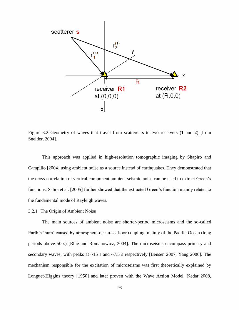
93
This approach was applied in high-resolution tomographic imaging by Shapiro and
Campillo [2004] using ambient noise as a source instead of earthquakes. They demonstrated that
the cross-correlation of vertical component ambient seismic noise can be used to extract Green’s
functions. Sabra et al. [2005] further showed that the extracted Green’s function mainly relates to
the fundamental mode of Rayleigh waves.
3.2.1 The Origin of Ambient Noise
The main sources of ambient noise are shorter-period microseisms and the so-called
Earth’s ‘hum’ caused by atmosphere-ocean-seafloor coupling, mainly of the Pacific Ocean (long
periods above 50 s) [Rhie and Romanowicz, 2004]. The microseisms encompass primary and
secondary waves, with peaks at ~15 s and ~7.5 s respectively [Bensen 2007, Yang 2006]. The
mechanism responsible for the excitation of microseisms was first theoretically explained by
Longuet-Higgins theory [1950] and later proven with the Wave Action Model [Kedar 2008,
Figure 3.2 Geometry of waves that travel from scatterer s to two receivers (1 and 2) [from
Sneider, 2004].

94
2011]. According to this theory, the interaction between two opposite waves will generate a
standing wave; the center of mass in the water column of a standing wave will rise twice per
cycle with respect to its equilibrium, and the vertical pressure of the column will produce seismic
wave at the bottom. However, two conditions must be met to excite seismic waves: 1. wave
trains driven by opposing winds over an ocean region must be of the same wavelengths; 2. the
depth of water column needs to be right for near acoustic resonance. The Longuet-Higgins
theory explains the excitation of Rayleigh and Stoneley waves (waves that travel along the
bottom of the ocean) by oceanic microseisms. The generation of Love waves is also possible due
to topographic effects and multipathing.
Kedar et al. [2008] found different causes for microseisms in the North Pacific and North
Atlantic oceans. A deep North Pacific Ocean is a less efficient deep-microseismic generator than
the North Atlantic and the source of microseisms is dominated by near-coastal wave-wave
interaction of oceanic swells [Kedar 2011, Yang et al., 2006]. In contrast, the North Atlantic
Ocean has depths that are more favorable for near acoustic resonance and is the dominant source
of ambient noise over North America and Western Europe during the fall and winter. The
dominant source was located near the southern tip of Greenland and related to deep ocean
sources, possibly caused by combinations of strong storms (cyclones), topographic effects on
wind patterns (southward deflection of wind by the high terrain) and local bathymetry [Kedar
2011].

95
3.3 Methods
3.3.1 Ambient noise tomography
3.3.1.1 Data Processing
I used a dataset collected from three regional contemporary broadband deployments,
PULSE (PerU Lithosphere and Slab Experiment) [Eakin et al., 2014], CAUGHT (Central
Andean Uplift and Geodynamics of High Topography) [Ward et al. 2013], PERUSE (Peru Slab
Experiment) [Phillips and Clayton, 2014], together with global seismic network stations in the
area (Figure 3.1). In total, records from 130 seismic stations deployed over a three-year period
from 2011 to 2013 were used in this study.
To process the data, I follow the procedure described by Bensen et al., 2007 [Figure 3.3].
I used all available vertical component seismograms recorded between 2011 and 2013. The
instrument responses are removed because seismic stations used in the study have different types
of sensors. The records are cut into day-long segments, decimated to 1 sample per second and
band-passed filtered from 5 to 150s. The discrete signals (such as earthquakes or explosions) and
instrumental irregularities are removed by applying temporal normalization. This is done by
computing the weighted running average of the seismogram envelope for the time window of
fixed length, 20s. Spectral whitening follows the temporal normalization. This is done by
converting the data into the frequency domain using Fast Fourier Transform (FFT) and applying
spectral whitening to broaden the band of the ambient noise signal and avoid the effects of
monochromatic sources.

96
In the next step I calculated the daily cross-correlations for each station pair and stacked
them over the entire period of time. Only records with >80 per cent of the day were used. Cross-
correlations for station FS13 are shown on Figure 3.4 with an apparent increasing time lag as the
inter-station distance increases. The full cross-correlation waveform is a two-sided time function
with positive and negative signals offset from zero by the same amount of time, that correspond
to waves that travel in opposite directions between two stations. Any dissymmetry of positive
and negative lags can arise from an inhomogeneous distribution of ambient noise sources.
However, in spite of different waveforms, the travel time is almost the same with the average
uncertainty of 1 s for periods shorter than 24 s [Lin et al., 2008]. This allows stacking of the two
Figure 3.3 Schematic representation of the data processing scheme (after Bensen et al., 2007).
Phase I
Phase II
Phase III
Phase IV
Raw data Remove instrument response, remove
mean and trend, band-pass filter, cut
to length of 1 day
Apply time domain
normalization
Apply spectral
whitening
Compute cross-
correlation
Stack day-correlations to
desired number of days
Measure group and/or
phase velocity
Error analysis Selection of acceptable
measurements

97
components into a one-sided signal by averaging the positive and negative components. This
process greatly increases signal-to-noise ratio (SNR) of the observed signal and additionally
contributes to greater homogeneity of the source distribution. In this case the SNR can be
regarded as the ratio between the maximum amplitude of the signal and amplitude r.m.s. [Warren
et al. 2013]. In further steps all the cross-correlations with SNR less than 15 were discarded
[Warren et al. 2013].

98
Next step includes measuring group and phase velocities using automated dispersion
measurements that rely on traditional automated frequency-time analysis (FTAN) [Levshin et al.,
Figure 3.4 Stack of daily cross-correlations for station FS13. a) All cross-correlations. b) Zoomed
first 10 cross-correlations

99
1989, Levshin and Ritzwoller, 2001]. This involves the filtering of signals over narrow
bandwidths centered at the frequency of interest. In order to get reliable phase velocity
measurements, the interstation spacing needs to be at least 3 wavelengths. Hence, the periods for
which phase velocities can be determined between a specific station pair is governed by
interstation distance, and the longest period for which reliable measurements can be obtained in
this study is 40s. Thus, in this step all measurements that do not fulfill this condition were
discarded.
The fourth step includes quality control and error analysis. Besides discarding the
measurements with interstation distance less than 3 wavelengths and cross-correlations with
SNR less than 15, all dispersion measurements with apparent average phase velocities above 5
km/s and below 1.5 km/s were removed. In this way, all obvious outliers have been discarded.
The summary of the obtained and rejected cross-correlations for periods ranging from 6
to 40 s is shown in Table 3.1. Periods from 8 to 30 s have the most useable data. The number of
ray paths rejected due to poor signal-to-noise ratio rapidly increases above 25 s. The SNR is not
governed by greater interspatial distance alone, but also by the strength of the source. Figure 3.5
shows the rose diagrams with the remaining paths, whereas the red lines illustrate the SNR
between two stations. The high SNR observed at shorter periods indicates a much stronger
source of the ambient noise than at longer periods. However, longer periods are associated with
more heterogeneous sources than the short periods. The source from NE direction (Atlantic
Ocean, Mexican Bay) dominates over the shortest periods.

100
Description 6 8 10 12 15 18 20 25 28 30 33 35 40
Total number of waveforms 625 5220 5935 6215 6593 6696 6603 5846 5206 4558 3825 3331 2596
After rejection of signal with SNR<15 495 4882 5342 6181 6538 6623 5070 3879 3073 2439 1716 1282 674
After rejection of signals with distance <3λ and time residuals >3s 464 4100 4471 4495 4495 4237 3891 2156 2156 2156 954 590 222
Remaining (%) 74 78 75 72 68 63 59 37 41 47 23 18 9
Table 3.1 Number of cross-correlated paths used in the study.
As a final step in the quality control, all paths with time residuals greater than 3 s were
removed [Warren et al., 2013; Ward et al., 2013]. Figure 3.6 shows the remaining paths used
further in the study. Finally, due to poor path coverage, periods shorter than 8 s and longer than
30 s were not further used in the inversion for shear wave velocities.

101
Figure 3.5 Azimuthal distribution of the source inferred from the SNR ratio between two stations
for periods 8,15,33, and 40 s. Red lines indicate SNR between two stations. The grid spacing of
circles is 15.

102
Figure 3.6 The remaining ray paths obtained for periods from 6 to 40 s. Black dots are stations
used in the study. Red triangles are Holocene volcanoes
103
3.3.1.2 Ambient noise phase velocity inversion
Phase velocities along interstation paths can be combined together to get dispersion
curves at previously defined grid nodes following the procedure of Barmin et al. [2001]. Here,
the 2-D isotropic phase velocity model is determined by minimizing a penalty function that
consists of data misfit and model smoothness, as well as constraints on model curvature:
(𝐆(𝐦) − 𝐝)𝑇𝐂−1(𝐆(𝐦) − 𝐝) + 𝛼2‖𝐅(𝐦)‖2 + 𝛽‖𝐇(𝐦)‖2 (3.1)
where G is the forward operator computing travel times from the starting model, d is the data
vector that consists of observed travel time residuals with respect to the starting model, m is the
model, C is the data covariance matrix assumed here to be diagonal and composed of the square
of the measurement standard deviations, F(m) is the spatial smoothing function with smoothing
width σ, and H(m) penalizes the model based on path density and azimuthal distribution. The
spatial smoothing is additionally controlled by the regularization parameters: α and β which
control the damping and the averaging of data in regions with poor path coverage, respectively.
The regularization parameters are determined by trial and error [Barmin, et al. 2001]. While most
previous studies use β = 100 and σ between 50 and 100 [e.g. Warren et al., 2013; Porter et al.,
2012; Ward et al, 2013], their α values vary greatly. Using high α values results in too smooth
images, while the lower values may produce spurious features (Figure S3.1). Ultimately, a
combination of α = 400, β = 100, and σ = 100 km yielded a model with lateral variations
appropriate for the given station coverage, avoiding the introduction of artifacts.
Grid node spacing has similar effects on the final results: greater distance between grid
nodes yields smother results with smaller-amplitude features. I tested models with grid node
104
spacing ranging from 1° to 0.1° (Figure S3.2). My final model uses 0.25º grid node spacing. This
grid produces detailed maps without introduction of apparent artifacts.
To test the sensitivity of calculated phase velocities to a priori information, I used
starting models with uniform starting value (1D starting models) and 2D starting models. The 2D
starting model was created by predicting the phase velocities using forward algorithm of Saito
[1988] for the velocity structure comprised from crustal velocities developed by James [1971]
and the IASPEI91 model for the mantle [Kenneth, 1991]. The resulting models are shown in
Figure 3.7. In the region with a lot of crossing paths within the station array (Figure 3.6) the
differences between the resulting phase velocities are negligible (Figure 3.8). In contrast, in the
areas with lack or no crossing paths (Figure 3.6), the differences in the obtained models are
profound. In these poorly resolved areas the obtained models reflect the starting phase velocities.
This test demonstrates that the obtained phase velocities within the area with good resolution are
robust and have limited sensitivity to starting values.

105
3.3.2 Iterative, rank equalized joint inversion for shear wave velocity
A finite-frequency two-plane wave method was used to invert for 12 periods in the band
between 0.007 Hz and 0.03 Hz (Forsyth and Li [2005]; Yang and Forsyth [2006]) and algorithms
of Saito [1988] and Weereratne et al. [2007] to invert for the shear wave velocities. The methods,
dataset and data processing have been described in Chapter II. In addition, in this study I employ
an iterative, rank-equalized approach [Rau and Forsyth, 2011]. Each iteration is a two-step
Figure 3.7 Sensitivity of calculated phase velocities for the periods of 25s, 28s, and 30s to the
starting models. Black circles are stations used in the study. Red triangles are Holocene
volcanoes. Colors and contour lines indicate phase velocities in km/s.

106
procedure and involves both phase and shear wave velocity inversions. The resulting shear wave
velocities and predicted phase velocities are used as starting models in the next iteration.
The iterative, rank-equalized approach can improve the resulting shear wave velocity
model by dealing with two major issues. The first is related to the effects of damping on the final
phase velocities. Typically, damping is applied to regularize the inversion and avoid short
wavelength artifacts. However, it often results in underestimation of the modeled amplitudes
[Aster, Borchers and Thurber, 2011]. In the iterative approach, the first step of the Rayleigh
wave phase velocity inversion uses a coarse grid, while the inversion is held underdamped. The
coarse grid in the first iteration results in a smooth model, without short wavelength artifacts,
while by underdamping the inversion one avoids underestimation of the model amplitude. The
resulting dispersion curves are inverted for the shear wave velocity structure and the predicted
phase velocities are used as the starting model in the following iteration. The grid is refined with
each iteration, yielding the final model with better-constrained absolute phase velocities.
The second issue relates to the inversion for shear wave velocities. Due to their broad
sensitivity kernels (Figure 3.8), longer periods are less well resolved than shorter periods and
may not resolve the amplitude of anomalies as well as shorter periods do. This may yield
artifacts in the 1D shear wave velocity model because shallow anomalies well resolved by
shorter periods will appear weaker at longer periods. The inversion resolves this by adding an
artifact at greater depths with an opposite polarity of the shallower anomaly. With rank
equalization, however, one can avoid these artifacts in the vertical velocity structure [Rau and
Forsyth, 2011]. This is because the smoothing applied to the longer periods is reduced
sufficiently that the rank (resolution power) of these periods is amplified to match those of
shorter periods.

107
In the first iteration, the starting phase velocities were found by predicting the dispersion
curve for the model that consists of velocity model of James [1971] for the crust and the
IASPEI91 for the mantle [Kenneth, 1991] (Figure 1.5, Chapter I). The a priori model
incorporates different crustal thicknesses across the study area. The crustal thickness was
adopted from Tassara et al., [2006], but smoothed along the coast to account for coupling of the
subducting and overriding plates in the forearc (Figure 1.6). A coarse, 1.2° grid node spacing
was applied in the first iteration. In the following iterations the grid was refined, first to 0.66°,
and later to 0.5°, which allowed for the modelling of finer features (Figure S3.3). Ranks were
equalized based on period with the highest rank, and the other periods are inverted until their
rank reached ± 1% of that value. In the last iteration, the phase velocity inversions at the longest
periods (111, 125, 143 s) became unstable when smoothing was sufficiently reduced to reach
rank equalization and were therefore not included in the final shear inversion. However, since
those periods were included in the shear wave velocity inversion in the second iteration, which
became a starting model for the final inversion, information from the long periods is still
incorporated in the final shear wave velocity model.
In the shear inversion, I jointly invert ambient noise with earthquake generated Rayleigh
wave phase velocities (21 periods in total). These periods are sensitive to shear wave velocity
structure between ~5 and ~200 km depth (Figure 3.8). The a priori shear wave velocity model
used in the first iteration has IASPEI91 velocities for the mantle [Kenneth, 1991]. I used the
uniform starting crustal model for the shear wave inversion instead of using model of James
[1971]. I found that using a layered crustal starting model tended to produce artifacts. During
each step the shear velocities were allowed to vary, but the layer thickness was held constant.

108
The shear inversion was regularized in part with model covariances obtained from the
two-plane wave method [Forsyth and Li, 2005]. For the ambient noise phase velocities, model
covariances are not available from the phase velocity inversions. Therefore, the regularization of
these parameters in the shear inversions was based on the spatial resolution maps of the ambient
noise phase inversions [Figure 3.9]. These show the highest resolution within the station array
and little to no resolution beyond the array. For areas where the spatial resolution was ≤ 30 km,
the covariance was set to 1% of the velocity; if the spatial resolution varied between 30 and 50
km the covariance was set to 1.11%; and if the spatial resolution was > 50 km, the covariance
was set to 3.33% (Figure S3.4). In this manner phase velocities in poorly resolved areas were
allowed to vary more.

109
3.4. Resolution
3.4.1 Lateral resolution of ambient noise phase velocities
The resolution matrix of ambient noise phase velocities was used to define spatial
resolution maps (Figure 3.9) [Lin et al., 2008]. The spatial resolution at each grid point
represents the distance at which amplitude of the 2D symmetric Gaussian function placed at the
node reduces to one-tenth [Lin et al., 2008; Warren et al., 2013]. The Figure 3.9 shows that I am
Figure 3.8 Sensitivity kernels for periods used in the study
0
50
100
150
200
250
300
0.000 0.020 0.040 0.060 0.080
8
10
12
15
18
20
25
28
30
33
40
45
50
58
66
77
91
100
111
125
143
Sensitivity
Depth
(km
)

110
able to resolve features as small as ~30 km in the areas with good ray coverage, and ~50km in
areas with smaller amount of crossing paths but within the station array (Figure 3.6).
Figure 3.9 Spatial resolution of periods used in the study. Colors and contour lines indicate
spatial resolution in km. Black dots are stations used in the study. Red triangles are Holocene
volcanoes.

111
3.4.2 Lateral resolution of phase velocities after final iteration
To test how the lateral resolution of earthquake-generated Rayleigh waves varies across
the region, I examine the resolution matrix diagonal from the two-plane wave inversion (Figure
3.10). I also use the resolution matrix from the final iteration to estimate the recoverability of
imposed features through a series of checkerboard tests (Figure 3.11). The resolution matrix
diagonal shows the highest resolution in the Western Cordillera, Eastern Cordillera and Altiplano
(Figure 3.10). Recovery tests indicate that features can be fairly recovered in these areas (Figure
3.11).
The resolution along the coastal forearc, SubAndan Zone and foreland varies with
periods. In these areas the resolution matrix diagonals indicate some resolution, and the recovery
tests seem more successful in identifying well from poorly resolved areas (Figure 3.11). At
shorter periods (33-45 s) the recovery tests show evident smearing along the coast and no
resolution in foreland. The streaking along the coast could be caused by lack of data and/or
crossing ray paths. But, at long periods the input anomalies can be fully recovered in these areas,
even beyond the station array (Figure 3.11).

112
Figure 3.10 Resolution matrix diagonal of final earthquake-generated phase velocities.

113
Figure 3.11 Recovery tests of final earthquake-generated phase velocities.

114
3.4.3. Vertical resolution
The vertical resolution of the shear wave velocity model depends on the breadth of the
overlapping sensitivity kernels of periods used in the study, together with the layer thicknesses
used in the inversion. Figure 3.12 shows the resolution matrix diagonal from the final shear wave
velocity model for all inverted nodes. The color of plotted circles refers to mean resolution
matrix diagonal of each layer. The resolution rapidly drops beyond ~200 km depth. Between 200
and ~300 km the vertical resolution is limited because the longest periods (111s, 125s, 143s) are
very broad with depth.
Figure 3.12 Vertical resolution. Black lines represent the resolution matrix diagonal for all
inverted nodes. The color of circles represents the mean resolution matrix diagonal per layer.

115
3.4.4. Sensitivity to a priori crustal thickness
Another important parameter that can affect the shear wave velocity model is a priori
information on crustal thickness. Since the broad vertical sensitivity kernels of Rayleigh wave
phase velocities to shear wave velocity are not very good for identifying sharp velocity
boundaries [Lebedev, Adam, and Meier; 2013], it is important to combine the phase velocities
with a priori information on the Mohorovicic discontinuity. For this reason I test the sensitivity
of my results to a priori crustal thickness by introducing two different crustal thickness models.
One model is based on the gravity study of Tassara et al., [2006] and the other is based on
preliminary receiver functions calculated using data from the PULSE seismic network [Brandon
et al., 2015] (Figure S3.5). The models are mainly in agreement in the southern part of the study
area and the effects on my shear wave velocity model of switching from one to the other are
negligible (Figure S3.6d and S3.6e). However, significant differences appear between the two
models further to the north, where additional complexities, such as erosion of the subducting
margin, subduction of the Nazca Ridge [Hampel et al., 2002], and the slab tear [Antonijevic et
al., 2015] take place. I find that applying the thinner crust of Bishop et al., [2015] in these areas
has strong effects on my model as the strong mid-crustal anomalies start to appear in the lower
crust and uppermost mantle (Figure S3.6b and S3.6c). Since these effects occur in the areas with
limited receiver function coverage due to station locations, I chose to use crustal thickness after
Tassara et al. [2006]. Combining gravity and/or the final receiver function results of Bishop et al.
[2015] may improve the model for crustal thickness in this area in future.

116
3.5 Results
3.5.1 Ambient noise phase velocity maps
Figure 3.13 shows the phase velocity maps from the ambient noise inversions. The
obtained periods between 8s and 30s have peak sensitivities between ~5 and ~35 km depth. The
maps show a remarkable first-order correlation between the observed anomalies and major
morpho- structural units (Figure 3.1), especially at shorter periods. There are low velocity
anomalies located along the location of Tertiary volcanoes (Figure 3.13, periods 8-30 s).
Similarly, there are low velocities located in the region of the Subandean basin (Figure 3.13, at
periods 8-12 s). In contrast, the Precambrian basement and Paleozoic strata of the Eastern
Cordillera are co-located with high velocity anomalies that are surrounded by the low velocities
of the Western Cordillera to the west, and the Subandean Zone to the east (Figure 3.13 periods 8-
30 s). Faster velocities are also observed in the forearc region.
To the south, the western flank of the Altiplano Plateau and the eastern rim of the
Western Cordillera (Figure 3.13) co-locate with low phase velocities at all periods. At shorter
periods (8 -15 s) the prominent low velocities align with the Cuzco-Vilcanota fault system
(Figure 3.1). As oppose to fast velocities observed along the Eastern Cordillera to the north, to
the south the Eastern Cordillera correlates with generally lower phase velocities.

117
3.5.2. Earthquake-generated Rayleigh wave phase velocities
The final phase velocities obtained with the two-plane method are shown on Figure 3.14. In
spite of different approaches, the resulting phase velocity maps are consistent with previous
Figure 3.13 Final phase velocity maps from ambient noise tomography. Black circles are stations
used in the study. Red triangles are Holocene volcanoes. Colors and contour lines indicate phase
velocities in km/s.

118
results [Antonijevic et al., 2015; Antonijevic et al., 2016]. At shorter periods (33 and 40 s) the
low velocities correlate with the entire Western Cordillera, as well as with the Altiplano Plateau
and the Eastern Cordillera in the southern part of the study area. At intermediate periods (45, 50,
and 58 s), however, the lower velocities still persist to the south and north, while velocities
increase along the flat slab region, above the projected subducting Nazca Ridge (Figure 3.1). At
longer periods the flat slab region coincides with low phase velocities, consistent with previous
studies [Antonijevic et al., 2016]. North of the projected subducting Nazca Ridge intermediate
and long periods reveal low phase velocities that strike parallel to the trench. The low velocities
are bound by fast anomalies to the west and east. The fast anomaly to the west is parallel to the
trench and becomes more prominent with longer periods. The fast velocity anomaly to the east
shifts inboard with longer periods. The anomalies are consistent with previously proposed
foundered dipping slab to the west and flat slab remnants to the east [Antonijevic et al., 2015;
2016; Scire et al., 2016].

119
Figure 3.14 Earthquake-generated Rayleigh wave phase velocity maps. Black circles are stations
used in the study. Red triangles are Holocene volcanoes Colors and contour lines indicate phase
velocities in km/s. The longest periods (111 s, 125 s, and 143 s) are with broader (0.66°) grid node
spacing.
.

120
3.5.3. 3D shear velocity model
To the south, low velocity anomalies in the upper crust spatially collocate with the
Subandean basins, active volcanic arc and Cusco-Vilcanota fault system (Figure 3.15a and
3.15b). The pronounced low velocity anomaly in the Sub-Andean basin (at ~70°W, ~13°S)
occurs within the uppermost ~10-15 km depth (Figure 3.16b) and spatially coincides with the
short wavelength Bouguer anomaly [Fukao et al., 1989]. Fluids and thick unconsolidated
Quaternary sediments within the basin and Andean detachment fault may be responsible for the
strong velocity reduction in this area. Along the Cusco-Vilcanota fault system velocity reduction
is more prominent to the north at shallower depths [Figure 3.15a], while at greater depths it is
greater to the south [Figure 3.15b].
A profound low velocity anomaly is situated in the middle crust, between ~10 and ~25
km depth, and extends sub-parallel to the trench (Figure 3.15). At ~15 km depth it collocates
with the western edge of the Altiplano Plateau and eastern rim of the Western Cordillera (Figure
3.15b), but expands eastwards at greater depths (Figure 3.15c, 3.15d; Figure 3.16b). The
anomaly is consistent with previously observed ‘Andean Low Velocity Zone’ (ALVZ) [Ma and
Clayton, 2014; Ma and Clayton, 2015]. From the western end of the anomaly low velocities
ascend westward, towards active volcanic arc (Figure 3.16b). From the eastern end, the low
velocities ascend towards the inboard Quimsachata volcano, but also plunge eastward,
overlaying a fast velocity anomaly (Figure 3.16b). The ALVZ continues further north, along the
flat slab segment, but the velocity reduction diminishes to the north (Figure 3.15b). In contrast,
velocities in the lower crust decrease from north to south (Figure 3.15 c,d).
The along-strike profile reveals remarkable variations in the slab geometry (Figure
3.16c). To the south, under the active arc (Figure 3.16c, Figure S3.6d and S3.6e), the abundant
121
seismicity occurs at the top of the fast anomaly, illuminating the steeply dipping slab, that is
overlain by low velocities. Further north, the velocities ascend Figure 3.16c, “TS”), illuminating
the change in slab’s geometry from steep to flat. While along the transitioning slab the fast
velocities mainly appear under the plane of seismicity (Figure 3.16c, “TS”), along the flat slab
segment the fast velocities appear both above and under the plane of seismicity. North of the
subducting Nazca Ridge, dipping and sagging of plane of seismicity (Figure 3.16c, “T”)
illuminates complexities, consistent with recently inferred tearing slab [Antonijevic et al., 2015].

122
Figure 3.15 Shear wave velocity structure at a) 5km, b) 15km, c) 30 km, and d) 40 km depth.
Black circles are stations used in the study. Dark red triangles are Holocene volcanoes. Colors
and contour lines show shear wave velocities. Green dashed line in a) and b) refers to Cuzco-
Vilcanota fault system [after Chapman et al., 2015]. Area with spatial resolution >50km (Figure
3.9) has been masked. ALVZ – Andean Low Velocity Zone; white dashed line refers to
Huaylillas arc 24-10 Ma [after Mamani et al., 2010].

123
Figure 3.16 Tomographic cross-sections shown on Figure 3.1. a) A-A’ shows re-steepened slab.
b) B-B’ is along the segment where the slab changes its geometry. c) C-C’ is along-strike profile.
Large black circles are earthquakes from Kumar et al., [2016]; small dots are earthquakes from
ISC catalog. Red triangles are Holocene volcanoes. Black triangles are stations. Dashed line at b)
is the top of the slab [Ma and Clayton, 2015]. Orange triangle at c) is high heat flow [Uyeda et
al., 1980]. RS – re-steepened slab; FSR – flat slab remnant; ALVZ: Andean Low Velocity Zone;
Asth: asthenosphere; SB- Subandean Basin; T – tear; TS –transition in slab geometry from steep
to flat.

124
Further north, the fast anomaly is overlain by low velocities, similar to features observed
to the south, along the segment where the Nazca Plate subducts steeply. The northern profile
(Figure 3.16a) reveals that this fast anomaly dips eastward, next to dipping slow anomaly. The
features are consistent with recently reported re-steepened slab overlain by warm asthenosphere
[Antonijevic et al., 2015, 2016]. Figure 3.16a shows another fast anomaly to the east that aligns
with the plane of seismicity (Figure 3.16a, FSR anomaly). The feature is consistent with
previously proposed flat slab remnant that still persists to the east [Antonijevic et al., 2015,
2016].
3.6 Discussion
3.6.1 Slab flattening and inboard volcanism
Flattening of the subducting plate has been linked to the inboard spread of magmatism
since Coney and Reynolds [1977]. As the slab flattens, it causes the retreat of the asthenospheric
wedge, which results in the inboard migration of the volcanic arc. However, linking inboard
volcanism and slab flattening in southern Peru is rather challenging. Geochemical records
indicate the presence of widespread inboard volcanism in the past ~10 Ma [INGEMMET, 2016;
Chapman et al., 2015] (Figure 3.17) related to the formation of Altiplano Plateau [Kay and
Coira, 2009]. Nevertheless, several features associated with volcanism that occurred along the
Cuzco-Vilcanota fault system in the past ~4 Ma (Figure 3.17a and b, highlighted area) provide
evidence that connects some of this inboard volcanism to the flattening and southward migration
of the subducting plate relative to the overriding continent.
First, the geochemical records [INGEMMET, 2016; Chapman et al., 2015] show
volcanism that occurred near Cuzco along the northernmost flank of the Cuzco-Vilcanota fault
system (Figure 3.17a “C”, yellow triangle in the highlighted region, Figure 3.17b). This
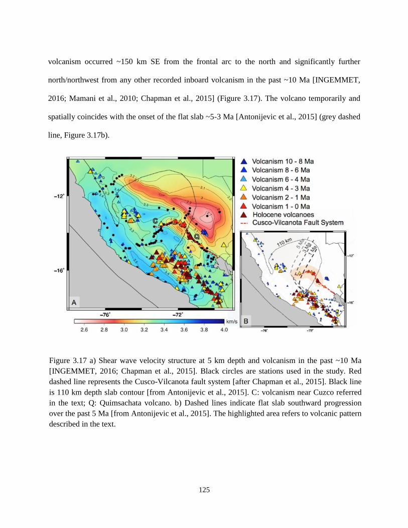
125
volcanism occurred ~150 km SE from the frontal arc to the north and significantly further
north/northwest from any other recorded inboard volcanism in the past ~10 Ma [INGEMMET,
2016; Mamani et al., 2010; Chapman et al., 2015] (Figure 3.17). The volcano temporarily and
spatially coincides with the onset of the flat slab ~5-3 Ma [Antonijevic et al., 2015] (grey dashed
line, Figure 3.17b).
Figure 3.17 a) Shear wave velocity structure at 5 km depth and volcanism in the past ~10 Ma
[INGEMMET, 2016; Chapman et al., 2015]. Black circles are stations used in the study. Red
dashed line represents the Cusco-Vilcanota fault system [after Chapman et al., 2015]. Black line
is 110 km depth slab contour [from Antonijevic et al., 2015]. C: volcanism near Cuzco referred
in the text; Q: Quimsachata volcano. b) Dashed lines indicate flat slab southward progression
over the past 5 Ma [from Antonijevic et al., 2015]. The highlighted area refers to volcanic pattern
described in the text.

126
Second, for the next ~4 Ma this inboard volcanism has been migrating southeast
(triangles in the highlighted area, Figure 3.17b), following the Cusco-Vilcanota fault system, and
ending with the Holocene eruptions of the Quimsachata volcano (Figure 3.17a “Q”) [Cabrera,
Sebrier, and Mercier, 1991; Chapman et al., 2015]. These Pliocene-Quaternary volcanics
exposed along the Cuzco-Vilcanota fault are characterized as high-potassium calc-alkaline lava
flows, ranging from basalt to rhyolites and referred to as the Quaternary Rumicolca formation
[Cabrera, Sebrier, and Mercier, 1991; Carlier et al., 1997; 2005; Chapman et al., 2015]. The
southeast migration of this inboard volcanism coincides with the direction of the flat slab
progression (Figure 3.17b). During this period of time the frontal arc ceased (yellow and orange
triangles at ~74.5ºW, ~13ºS, Figure 3.17) [INGEMMET, 2016], consistent with cooling effects
that accompanied slab flattening further north [e.g. Coney and Reynolds, 1977].
Third, the xenoliths from Pliocene-Quaternary ultrapotassic volcanic rocks along the
Cuzco-Vilcanota fault (triangles in the highlighted area, Figure 3.17b) are interpreted as most
likely recently derived from asthenospheric mantle due to their high 143Nd/144Nd (0.5126 -
0.5129) and lower 87Sr/86Sr (0.704 – 0.709) ratios [Chapman et al., 2015; Carlier et al., 2005].
My tomographic images show low velocities above the dipping fast velocities ~350 km away
from the trench (Figure 3.16b), which I attribute to asthenosphere overlaying the portion of the
slab that resumes a steeply dipping geometry. The low velocities continue throughout the entire
crust, ascending westward towards the inboard Quimsachata volcano. The ascending low
velocities might also indicate a deep mantle origin of this inboard volcano, consistent with
geochemical observations [Chapman et al., 2015; Carlier et al., 2005].
All these features suggest a connection between the southward progression of the flat slab
and the inboard volcanism highlighted in Figure 3.17b. However, even though the flat slab

127
started to form further north, at ~11°S [Rosenbaum et al., 2005], inboard volcanism did not
appear prior to eruptions along the Cusco-Vilcanota fault system (Figure 3.17). The absence of
inboard volcanism further north may suggest that pre-existing structures play an important role
in the appearance of inboard volcanism. The Cusco-Vilcanota fault system runs from Cuzco to
Lake Titicaca [Chapman et al., 2015] and represents a pre-Andean suture zone between two
lithospheric blocks [Carlier, 2005]. Historic seismicity inferred from the surface morphologies
along this fault show that the fault system has been recently active as a sinistral trans-tensional
fault [Sebrier et al., 1985]. The observed low velocities along the fault (Figures 3.15) indicate
that this weak trans-lithospheric zone may have served as a path of least resistance for ascending
melt/fluids through the thick Andean crust (~60-70 km). The connection between pre-existing
structures (faults) and volcanism has been observed in other settings worldwide, for example in
Lesser Antilles and Nicaragua [Mathieu et al., 2011], Deception Island (NW Antarctica) [Lopes
et al., 2015], Callaqui Stratovolcano in the Andean Southern Volcanic Zone (Central-Southern
Chile) [Sielfeld, Cembrano, and Lara; 2016]. These weak zones tend to control the location of
intrusives and hydrothermal activity, resulting in volcanism restricted to a particular area,
consistent with observations in southern Peru.
Another important question relates to generation of the inboard volcanism. Earlier studies
relate inboard volcanism in the flat slab regions to the point where the subhorizontally traveling
plate resumes to subduct steeply, and where the combination of asthenospheric heat and slab-
derived fluids can produce flux melting [e.g. Kay and Abruzzi, 1996]. This is consistent with
geophysical observations in southern Peru (Figure 3.16b). It is also consistent with geochemical
observations, since the composition of the Pliocene-Quaternary lavas collected along the Cusco-
Vilcanota fault system indicate volatile-rich melts of the mantle source [Carlier et al., 2005].

128
This would imply that the slab still releases fluids via metamorphic dehydration reactions ~350
km away from the trench, but aseismically, since the intermediate depth seismicity, which may
relate to slab dehydration (e.g., Kirby et al., 1996) terminates ~200-250 km away from the trench
(Figure 3.16b).
Observations of seismic anisotropy along the segment where the slab changes its
geometry from steep to flat to the south offer an additional possible explanation for the presence
of fluids within the asthenosphere this far to the east. The trench-parallel flow above the steeply
dipping slab to the south, inferred from local shear wave splitting [Long et al., 2016], may
continue further north and get deflected due to the sudden change in slab geometry (fast
directions parallel to slab contours as observed from Rayleigh wave phase anisotropy
[Antonijevic et al., 2016]). This flow would be consistent with modeling studies that showed that
along-strike variations in slab geometry may produce very complex patterns in the
asthenospheric wedge [Kneller and van Keken, 2007, 2008]. The arc related fluids could be
transported further north/northeast via this flow from the regions above the normally dipping
plate to the south. This complex flow may offer an explanation for the presence of volatiles
necessary to generate flux melting ~350 km away from the trench and back arc volcanism.
3.6.2 Andean Low-Velocity Zone, slab flattening and the cessation of arc volcanism
A profound middle crustal low velocity anomaly in southern Peru has been earlier
identified as the Andean Low-Velocity Zone (ALVZ) [Ma and Clayton, 2014, 2015]. Due to its
oblique orientation with respect to trench, the anomaly was associated with Huayillas arc that
was active between 24 and 10 Ma (Figure 3.15b, white dashed lines) [Ma and Clayton, 2014;
Mamani et al., 2010]. However, the low velocities ascending westward from the ALVZ towards
the active volcanoes (Figure 3.16b) also indicate connection between the ALVZ and the present-

129
day arc. High heat flow [Hamza et al., 2005] and reduced shear wave velocities imply presence
of partial melting under the present-day arc.
The ALVZ continues further north, along the flat slab region (Figure 3.15). The low
velocities above the flat slab spatially coincide with recently terminated volcanic arc (Figure 3.15
and Figure 3.17), reflecting the residual heat still trapped within the middle crust. However, a
distinctive increase in velocities from south, where the arc is active above the steeply dipping
slab, to the north, where the slab flattens, is noticeable (Figure 3.15 and b, Figure 3.16c, Figure
3.17). This pattern is consistent with progressive cooling and cessation of arc volcanism due to
the flattening of the subducting plate that first occurred to the north (Figure 3.17) [Hampel et al.,
2002, Rosenbaum et al., 2005, Antonijevic et al., 2015]. Deeper crustal structures along the
northernmost part of the study area, however, are associated with additional complexities due to
tearing slab north of the subducting Nazca Ridge [Antonijevic et al., 2015, 2016; Scire et al.,
2016].
3.6.3 Effects of the slab tear
In contrast to shallower crustal structures in the northern part of the study area, the
velocities in the lower crust decrease from south to north (Figure 3.15d, Figure 3.16c). The
absence of high velocities in the upper mantle and lower crust suggests that cooling effects due
to slab flattening are no longer present at these depths. Here, the tomographic images indicate
dipping slab (Figure 3.16a), consistent with recently reported torn and re-steepened slab
[Antonijevic et al., 2015; Scire et al., 2016]. The re-steepening of the subducting plate allows
inflow of warm asthenosphere between two plates [Antonijevic et al., 2015; 2016], which may
explain the observed dipping low velocities (Figure 3.16a).

130
The southward increase in velocities in the northern part of the study area (Figure 3.16c)
is consistent with the tear that has been propagating from north to south. While the nature of the
flat slab or tear is unknown north of the study area, the earthquake distribution indicates a gap in
seismicity that continues further north [Antonijevic et al., 2015], illuminating a possible
continuation of the slab tear. Moreover, a recent study finds unusual 3He/ 4He in the samples
from hot springs of Cordillera Blanca (at ~9ºS), indicating the presence of up to ~25% mantle-
derived helium [Newell et al., 2015]. They speculate that one possible explanation for the
unusual input of He from mantle in this presumably flat slab region is tear-related. Future
imaging of structures further north is necessary to establish the northernmost extent of the slab
tear and its effects on the overriding plate.
3.7 Conclusion
Comparing the shear wave velocity model, obtained for depths between 5 and 200 km,
with geochemical records on volcanism in the past ~10 Ma, I re-evaluate the volcanic patterns
during slab flattening. I provide additional, geophysical evidence for the connection between slab
flattening and the cessation in arc volcanism at the surface. Slab flattening forces corner flow to
retreat, resulting in thermal shielding and the termination of arc volcanism. The increase in
velocities under the recently terminated arc above the flat slab reflects progressive cooling due to
slab flattening that first occurred to the north. In contrast, appearance of low velocities in the
upper mantle and lower crust to the north, where the slab tears and re-steepens [Antonijevic et
al., 2015; Scire et al., 2015], indicates that the cooling effects are no longer present in this area
and that re-steepening of the slab allows inflow of the asthenosphere and heating of overriding
lithosphere from below.

131
The relationship between the slab flattening and inboard volcanism is more complex.
First, it requires volatile-rich asthenosphere that can produce flux melting. Second, it depends on
pre-existing zones of weaknesses within the overriding plate that play an important role in heat
and fluid transfer. These zones can facilitate and channelize the magmatic and hydrothermal
activity, resulting in volcanism restricted to a particular area. These findings have important
implications not only for better understanding the extent and geometry of the paleo-flat slabs
(e.g. during the Laramide orogeny in Western United States), since their extent and geometry are
usually inferred from volcanic patterns, but for all settings with active magmatism.

132
REFERENCES
1. Antonijevic, S. K., Wagner, L. S., Kumar, A., Beck, S. L., Long, M. D., Zandt, G.,
Hernando Tavera, and Cristobal Condori, C. (2015). The role of ridges in the formation
and longevity of flat slabs. Nature, 524(7564), 212-215.
2. Antonijevic, S. K., Wagner, L. S., Beck, S. L., Long, M. D., Zandt, G., Tavera, H. Effects
of Change in Slab Geometry on the Mantle Flow and Slab Fabric in Southern Peru.
Submitted to Journal of Geophysical Research: Solid Earth.
3. Aster, R. C., Borchers, B., & Thurber, C. H. (2011). Parameter estimation and inverse
problems (Vol. 90). Academic Press.
4. Barazangi, M., & Isacks, B. L. (1976). Spatial distribution of earthquakes and subduction
of the Nazca plate beneath South America. Geology, 4(11), 686-692.
5. Barmin, M.P., M.H. Ritzwoller, and A.L. Levshin, (2001), A fast and reliable method for
surface wave tomography, Pure Appl. Geophys., 158(8), 1351 – 1375.
6. Bensen, G. D., M. H. Ritzwoller, M. P. Barmin, A. L. Levshin, F. Lin, M. P. Moschetti, N.
M. Shapiro, and Y. Yang (2007). Processing seismic ambient noise data to obtain reliable
broad-band surface wave dispersion measurements. Geophysical Journal International,
169(3), 1239-1260.
7. Bishop, B. (2015, December). Modification of Thickened Orogenic Crust by a Subducting
Ridge: Disruption of the Andean Lower Crust of Southern Peru by the Subducting
Aseismic Nazca Ridge. In 2015 AGU Fall Meeting..
8. Cabrera, J., Sébrier, M., & Mercier, J. L. (1991). Plio-Quaternary geodynamic evolution
of a segment of the Peruvian Andean Cordillera located above the change in the
subduction geometry: the Cuzco region. Tectonophysics, 190(2), 331-362.
9. Carlier, G., Lorand, J. P., Audebaud, E., & Kienast, J. R. (1997). Petrology of an unusual
orthopyroxene-bearing minette suite from southeastern Peru, Eastern Andean Cordillera:
Al-rich lamproites contaminated by peraluminous granites. Journal of Volcanology and
Geothermal Research, 75(1-2), 59-87.
10. Carlier, G., Lorand, J. P., Liégeois, J. P., Fornari, M., Soler, P., Carlotto, V., & Cardenas,
J. (2005). Potassic-ultrapotassic mafic rocks delineate two lithospheric mantle blocks
beneath the southern Peruvian Altiplano. Geology, 33(7), 601-604.
11. Chapman, A. D., Ducea, M. N., McQuarrie, N., Coble, M., Petrescu, L., & Hoffman, D.
(2015). Constraints on plateau architecture and assembly from deep crustal xenoliths,

133
northern Altiplano (SE Peru). Geological Society of America Bulletin, 127(11-12), 1777-
1797.
12. Coney, P. J., & Reynolds, S. J. (1977). Cordilleran benioff zones. Nature, 270, 403-406.
13. DeMets, C., Gordon, R. G., & Argus, D. F. (2010). Geologically current plate motions.
Geophysical Journal International, 181(1), 1-80. doi: 10.1111/j.1365-246X.2009.04491.x
14. Dougherty, S. L., & Clayton, R. W. (2014). Seismic structure in southern Peru: evidence
for a smooth contortion between flat and normal subduction of the Nazca Plate.
Geophysical Journal International, 200(1), 534-555. http://dx.doi.org/10.1093/gji/ggu415
15. Eakin, C. M., Long, M. D., Beck, S. L., Wagner, L. S., Tavera, H., & Condori, C. (2014).
Response of the mantle to flat slab evolution: Insights from local S splitting beneath Peru.
Geophysical Research Letters, 41(10), 3438-3446.
16. Eakin, C. M., Long, M. D., Beck, S. L., Wagner, L.S., Tavera, H. & Condori, C. Upper
mantle anisotropy beneath Peru from SKS splitting: Constraints on flat slab dynamics and
interaction with the Nazca Ridge. Earth planet. Sci. Lett., 412 (2015): 152-162.
doi:10.1016/j.epsl.2014.12.015
17. Eakin, C. M., Long, M. D., Scire, A., Beck, S. L., Wagner, L. S., Zandt, G., & Tavera, H.
(2016). Internal deformation of the subducted Nazca slab inferred from seismic
anisotropy. Nature Geoscience, 9(1), 56-59. doi: 10.1038/ngeo2592.
18. Forsyth, D. W., and Li, A. Array analysis of two-dimensional variations in surface wave
phase velocity and azimuthal anisotropy in the presence of multipathing interference. In:
Levander, A. Nolet, G. (Eds), Seismic Earth: Array of broadband seismograms,
Geophysical Monograph Series 157, 81-98 (2005).
19. Fukao, Yoshio, Akihiko Yamamoto, and Masaru Kono (1989). "Gravity anomaly across
the Peruvian Andes." Journal of Geophysical Research: Solid Earth (1978–2012) 94.B4
20. Gutscher, M. A., Maury, R., Eissen, J. P., & Bourdon, E. (2000). Can slab melting be
caused by flat subduction?. Geology, 28(6), 535-538.
21. Hampel, A. (2002). The migration history of the Nazca Ridge along the Peruvian active
margin: a re-evaluation. Earth and Planetary Science Letters, 203(2), 665-679.
22. Hamza, V. M., Dias, F. J. S., Gomes, A. J., & Terceros, Z. G. D. (2005). Numerical and
functional representations of regional heat flow in South America. Physics of the Earth
and Planetary Interiors, 152(4), 223-256.

134
23. Humphreys, E., Hessler, E., Dueker, K., Farmer, G. L., Erslev, E., & Atwater, T. How
Laramide-age hydration of North American lithosphere by the Farallon slab controlled
subsequent activity in the western United States. Int. Geol. Rev. 45(7), 575-595 (2003).
24. Instituto Geologico Minero y Metalurgico. On-line catalog. (INGEMMET,
http://www.ingemmet.gob.pe (2016).
25. International Seismological Centre. On-line Bulletin (ISC, http://www.isc.ac.uk (2012).
26. Jaillard, E., Hérail, G., Monfret, T., Díaz-Martínez, E., Baby, P., Lavenu, A., & Dumont,
J. F. (2000). Tectonic evolution of the Andes of Ecuador, Peru, Bolivia and northernmost
Chile. Tectonic Evolution of South America, 31, 481-559.
27. James, D. E. Andean crustal and upper mantle structure. J. Geophys. Res., 76(14), 3246-
3271 (1971).
28. James, D. E., & Sacks, I. S. (1999). Cenozoic formation of the Central Andes: a
geophysical perspective. Geology and ore deposits of the Central Andes, 7, 1-25.
29. Kay, S. M., & Abbruzzi, J. M. (1996). Magmatic evidence for Neogene lithospheric
evolution of the central Andean “flat-slab” between 30 S and 32 S. Tectonophysics,
259(1), 15-28.
30. Kay, S. M., & Coira, B. L. (2009). Shallowing and steepening subduction zones,
continental lithospheric loss, magmatism, and crustal flow under the Central Andean
Altiplano-Puna Plateau. Geological Society of America Memoirs, 204, 229-259.
31. Kedar, S., Longuet-Higgins, M., Webb, F., Graham, N., Clayton, R., & Jones, C. (2008,
March). The origin of deep ocean microseisms in the North Atlantic Ocean. In
Proceedings of the Royal Society of London: Mathematical, Physical and Engineering
Sciences (Vol. 464, No. 2091, pp. 777-793). The Royal Society.
32. Kedar, S. (2011). Source distribution of ocean microseisms and implications for time-
dependent noise tomography. Comptes Rendus Geoscience, 343(8), 548-557.
33. Kennett, B.L.N. IASPEI 1991 Seismological Tables. Bibliotech, Canberra, Australia
(1991).
34. Kim, Y., & Clayton, R. W. (2015). Seismic properties of the Nazca oceanic crust in
southern Peruvian subduction system. Earth and Planetary Science Letters, 429, 110-121.
35. Kirby, S., Engdahl, R. E., & Denlinger, R. (1996). Intermediate‐depth intraslab
earthquakes and arc volcanism as physical expressions of crustal and uppermost mantle
metamorphism in subducting slabs. Subduction top to bottom, 195-214. doi:
10.1029/GM096p0195

135
36. Kneller, E. A., & van Keken, P. E. (2007). Trench-parallel flow and seismic anisotropy in
the Mariana and Andean subduction systems. Nature, 450(7173), 1222-1225.
37. Kneller, E. A., & Van Keken, P. E. (2008). Effect of three‐dimensional slab geometry on
deformation in the mantle wedge: Implications for shear wave anisotropy. Geochemistry,
Geophysics, Geosystems, 9(1)
38. Kumar, A., Wagner, L. S., Beck, S. L., Long, M. D., Zandt, G., Young, B., ... & Minaya,
E. (2016). Seismicity and state of stress in the central and southern Peruvian flat slab.
Earth and Planetary Science Letters, 441, 71-80.
39. Lebedev, S., Adam, J. M. C., & Meier, T. (2013). Mapping the Moho with seismic surface
waves: A review, resolution analysis, and recommended inversion strategies.
Tectonophysics, 609, 377-394.
40. Levshin, A.L., Yanovskaya, T.B., Lander, A.V., Bukchin, B.G., Barmin, M.P., Ratnikova,
L.I. And Its, E.N., 1989. Seismic Surface Waves in a Laterally Inhomogeneous Earth, ed
Keilis-Borok, V.I. Kluwer, Norwell, Mass.
41. Levshin, A. L., and M. H. Ritzwoller. "Automated detection, extraction, and measurement
of regional surface waves." Monitoring the Comprehensive Nuclear-Test-Ban Treaty:
Surface Waves. Birkhäuser Basel, 2001. 1531-1545.
42. Lin, F. C., Moschetti, M. P., & Ritzwoller, M. H. (2008). Surface wave tomography of the
western United States from ambient seismic noise: Rayleigh and Love wave phase
velocity maps. Geophysical Journal International, 173(1), 281-298.
43. Long M. D., Biryol, C.B., Eakin, C.M., Beck, S. L., Wagner, L.S., Zandt, G., Minaya, E.
and Tavera, H. Overriding plate, mantle wedge, slab, and sub-slab contributions to seismic
anisotropy beneath the northern Central Andean Plateau. Submitted.
44. Lopes, F. C., Caselli, A. T., Machado, A., & Barata, M. T. (2015). The development of the
Deception Island volcano caldera under control of the Bransfield Basin sinistral strike-slip
tectonic regime (NW Antarctica). Geological Society, London, Special Publications,
401(1), 173-184.
45. Ma, Y., & Clayton, R. W. (2014). The crust and uppermost mantle structure of Southern
Peru from ambient noise and earthquake surface wave analysis. Earth and Planetary
Science Letters, 395, 61-70.
46. Ma, Y., & Clayton, R. W. (2015). Flat slab deformation caused by interplate suction force.
Geophysical Research Letters, 42(17), 7064-7072.
47. Mamani, M., Wörner, G., & Sempere, T. (2010). Geochemical variations in igneous rocks
of the Central Andean orocline (13 S to 18 S): tracing crustal thickening and magma

136
generation through time and space. Geological Society of America Bulletin, 122(1-2),
162-182.
48. Manea, V. C., Perez-Gussinye, M. & Manea, M. Chilean flat slab subduction controlled
by overriding plate thickness and trench rollback. Geology 40, 35–38 (2012).
49. Mathieu, L., de Vries, B. V. W., Pilato, M., & Troll, V. R. (2011). The interaction between
volcanoes and strike-slip, transtensional and transpressional fault zones: Analogue models
and natural examples. Journal of Structural Geology, 33(5), 898-906.
50. Phillips, K., Clayton, R. W., Davis, P., Tavera, H., Guy, R., Skinner, S., ... & Aguilar, V.
(2012). Structure of the subduction system in southern Peru from seismic array data.
Journal of Geophysical Research: Solid Earth, 117(B11).
51. Phillips, K., & Clayton, R. W. Structure of the subduction transition region from seismic
array data in southern Peru. Geophys. J. Int. ggt504 (2014).
52. Porter, R., Gilbert, H., Zandt, G., Beck, S., Warren, L., Calkins, J., Alvarado, P. and
Anderson, M., (2012). Shear wave velocities in the Pampean flat‐slab region from
Rayleigh wave tomography: Implications for slab and upper mantle hydration. Journal of
Geophysical Research: Solid Earth, 117(B11).
53. Rau, C. J., & Forsyth, D. W. (2011). Melt in the mantle beneath the amagmatic zone,
southern Nevada. Geology, 39(10), 975-978.
54. Rhie, J., and B. Romanowicz, Excitation of earth's incessant free oscillations by
atmosphere-ocean-seafloor coupling, Nature, 431, 552-556. 2004.
55. Rosenbaum, G., Giles, D., Saxon, M., Betts, P. G., Weinberg, R. F., & Duboz, C. (2005).
Subduction of the Nazca Ridge and the Inca Plateau: Insights into the formation of ore
deposits in Peru. Earth and Planetary Science Letters, 239(1), 18-32.
56. Sabra,G.G , P. Gerstoft, P. Roux, W. A. Kuperman, and M. C. Fehler. 2005. Extracting
time-domain Green's function estimates from ambient seismic noise . Geophysical
Research Letters, vol. 32, L03310, doi:10.1029/2004GL021862.
57. Saito, M. DISPER80: a subroutine package for the calculation of seismic normal mode
solutions. In: Doornbos, D.J. (Ed.), Seismological Algorithms: Computational Methods
and Computer Programs. Elsevier, 293–319 (1988).
58. Scire, A., Zandt, G., Beck, S., Long, M., Wagner, L., Minaya, E., & Tavera, H. (2016).
Imaging the transition from flat to normal subduction: variations in the structure of the
Nazca slab and upper mantle under southern Peru and northwestern Bolivia. Geophysical
Journal International, 204(1), 457-479. doi: 10.1093/gji/ggv452

137
59. Sébrier, M., Mercier, J. L., Mégard, F., Laubacher, G., & Carey‐Gailhardis, E. (1985).
Quaternary normal and reverse faulting and the state of stress in the central Andes of south
Peru. Tectonics, 4(7), 739-780.
60. Sielfeld, G., Cembrano, J., & Lara, L. (2016). Transtension driving volcano-edifice
anatomy: Insights from Andean transverse-to-the-orogen tectonic domains. Quaternary
International. doi:10.1016/j.quaint.2016.01.002
61. Shapiro, N.M. M. Campillo, L. Stehly, and M.H. Ritzwoller (2005), High resolution
surface wave tomography from ambient seismic noise, Science, 307(5715), 1615-1618, 11
March 2005.
62. Snieder, R.A. (2004), Extracting the Green’s function from the correlation of coda waves:
A derivation based on stationary phase, Phys. Rev., 69, 046610-1-8.
63. Tassara, A., Go ̈tze, H.J., Schmidt, S. & Hackney, R., 2006. Three-dimensional density
model of the Nazca plate and the Andean continental margin, J. Geophys. Res., 111,
doi:10.1029/2005JB003976.
64. Uyeda, S., Watanabe, T., Ozasayama, Y. & Ibaragi, K. Report of heat flow measurements
in Peru and Ecuador. Bull. Earthquake Res. Inst. 55, 55–74 (1980).
65. van Hunen, J., Van Den Berg, A. P. & Vlaar, N. J. On the role of subducting oceanic
plateaus in the development of shallow flat subduction. Tectonophysics 352,317–333
(2002).
66. Ward, K. M., Porter, R. C., Zandt, G., Beck, S. L., Wagner, L. S., Minaya, E., & Tavera,
H. Ambient noise tomography across the Central Andes. Geophys. J. Int. 194(3), 1559-
1573 (2013).
67. Weeraratne, D. S., Forsyth, D. W., Fischer, K. M., & Nyblade, A. A. Evidence for an
upper mantle plume beneath the Tanzanian craton from Rayleigh wave tomography. J.
Geophys. Res.: Solid Earth. (1978–2012), 108(B9) (2003).
68. Warren, L. M., Beck, S. L., Biryol, C. B., Zandt, G., Özacar, A. A., & Yang, Y. (2013).
Crustal velocity structure of Central and Eastern Turkey from ambient noise tomography.
Geophysical Journal International, ggt210.
69. Yang, Y., Forsyth, D. W. Regional tomographic inversion of the amplitude and phase of
Rayleigh waves with 2-D sensitivity kernels. Geophys. J. Int. 166, 1148-1160 (2006).
70. Yang, Y., Ritzwoller, M. H., Levshin, A. L., & Shapiro, N. M. (2007). Ambient noise
Rayleigh wave tomography across Europe. Geophysical Journal International, 168(1),
259-274.

138
APPENDIX 1
Figure S1.1 Average root mean square misfit over all periods between observed and predicted
dispersion curves in shear wave inversion using 0.2 and 0.15 for damping in Rayleigh wave
phase inversion. Colors and contour lines show the misfit.

139
APPENDIX 2
Figure S2.1 Rose diagrams showing back-azimuthal distribution of the well recorded teleseismic
events with magnitude >6.2 during PULSE deployment.

140
.
Figure S2.2 Starting and calculated Rayleigh wave phase velocities for 40, 66 and 91 s. Colors
and contours indicate absolute phase velocities. Red triangles are Holocene volcanoes. Black
rectangles, circles and stars are stations used in the study.

141
Figure S2.3 Recovery tests for the velocity reduction due to partial melting. a) Observed
dispersion curve (purple triangles) with error bars representing one standard deviation of
uncertainty. Blue dots represent the dispersion curve that corresponds to starting model shown
with blue line at c). Red circles show the best fit to the observed dispersion curve yielding 1D
shear wave velocity model shown with red line at c). b) Suit of starting models with introduced
low velocities corresponding to 1% and 2% partial melting [Humpherys and Hammond, 2000]
for which predicted dispersion curves fit the observations within the confidence limits. c)
Recovered models (black lines) using predicted dispersion curves from 1D shear wave velocity
models shown at b) and our regular starting model (blue line). Red line represents the model
obtained using observed dispersion curve.

142
APPENDIX 3
Figure S3.1 Sensitivity of phase velocity results to varying regularization parameters. The first
value is α, and second value is β. Black circles are stations used in the study. Red triangles are
Holocene volcanoes. Colors and contour lines indicate phase velocities in km/s.

143
Figure S3.2 Effects of grid node spacing. Black circles are stations used in the study. Red
triangles are Holocene volcanoes. Colors and contour lines indicate phase velocities in km/s.

144
Figure S3.3 Phase velocities obtained for periods 45, 58, and 91 s after each iteration.

145
Figure S3.4 Data covariance used in shear wave velocity inversion for ambient noise (8-30s)
and shorter earthquake-generated Raleigh wave phase velocities (33-45 s).

146
Figure S3.5 Models used to test sensitivity of the shear model to crustal thickness: a) after
Tassara et al. [2006] modified along the coast; b) after Bishop et al. [2015].

147
Figure S3.6 Effects of different crustal thickness models on my final shear wave velocity
model: a) Reference map; b) and d) model after Tassara et al. [2006], c) and e) model after
Bishop et al. [2015]. Large black circles are earthquake locations from Kumar et al., [2016];
small dots are earthquake locations from ISC catalog. Colors and contour line represent absolute
shear wave velocities. Red triangles are Holocene volcanoes. Black triangles are stations used in
the study