IMAGE PROCESSING - Computer Sciencewolberg/cs4165/doc/CSc470.pdf · 1 Introduction to Image...

COURSE NOTES:

IMAGE PROCESSING

George Wolberg

Department of Computer ScienceCity College of New York

New York, NY [email protected]

1

Introduction to Image Processing

Prof. George WolbergDept. of Computer ScienceCity College of New York

2Wolberg: Image Processing Course Notes

Course Description

• Intense introduction to image processing.• Intended for advanced undergraduate and graduate students.

•Topics include:- Image enhancement- Digital filtering theory, Fourier transforms- Image reconstruction, resampling, antialiasing- Scanline algorithms, geometric transforms- Warping, morphing, and visual effects


Syllabus

Week12-345-67-89101112-14

TopicIntroduction / overviewPoint operationsNeighborhood operationsFast Fourier transforms (FFT)Sampling theoryMidterm, Image reconstructionFast filtering for resamplingSpatial transformations, texture mappingSeparable warping algorithms; visual effects


Texts

• Required Text:- George Wolberg, Digital Image Warping, IEEE

Computer Society Press, 1990.

• Supplementary Text:- Rafael Gonzalez and Richard Woods, Digital

Image Processing, 2nd Edition, Prentice Hall, Wesley, 2002.


Grading

•The final grade is computed as follows:- Midterm exam: 25%- Final exam: 25%- Homework programming assignments: 50%

•Substantial programming assignments are due every three weeks.

•Proficiency in C/C++ is expected.•Prereqs: CSc 30100 and CSc 32200


Computer Resources

• SUN Blade workstations (NAC 7/105)- Solaris 8 Operating System (UNIX)- OpenGL hardware support for fast rendering- 24-bit true-color graphics (16.7 million colors)

• Linux Lab (Steinman B41)- Red Hat OS (UNIX)- OpenGL hardware support for fast rendering- 24-bit true-color graphics (16.7 million colors)

• You can also program at home on your PC/laptop under MS Windows or Linux. Download MESA, if necessary, for Linux. Use C/C++ programming language.

2


Contact Information

•Prof. Wolberg- Office hours: After class and by appointment- Email: [email protected]

•Teaching Assistant (TA): Hadi Fadaifard- Email: [email protected]

•See class web page for all class info such as homework and sample source code:www-cs.ccny.cuny.edu/~wolberg/cs470 (CCNY)www-cs.ccny.cuny.edu/~wolberg/cs4165 (Columbia)


Objectives

•These notes accompany the textbooks:“Digital Image Warping” by George Wolberg“Digital Image Processing” by Gonzalez/Woods

•They form the basis for approximately 14 weeks of lectures.

•Programs in C/C++ will be assigned to reinforce understanding of the material.

- Four homework assignments- Each due in 3 weeks and requiring ~4 programs

What is Image Processing?

Prof. George WolbergDept. of Computer ScienceCity College or New York


Objectives

• In this lecture we:- Explore what image processing is about- Compare it against related fields- Provide historical introduction- Survey some application areas


What is Digital Image Processing?

• Computer manipulation of pictures, or images, that have been converted into numeric form. Typical operations include:

- Contrast enhancement- Remove blur from an image- Smooth out graininess, speckle, or noise- Magnify, minify, or rotate an image (image warping)- Geometric correction- Image compression for efficient storage/transmission


Image Processing Goals

• Image processing is a subclass of signal processing concerned specifically with pictures

• It aims to improve image quality for- human perception: subjective- computer interpretation: objective

• Compress images for efficient storage/transmission

3


Related Fields

Image Processing

SceneDescription

ComputerGraphics

ComputerVision

Image


Overlap with Related Fields

Image Processing

SceneDescription

ComputerGraphics

ComputerVision

Image

Low-level

Mid-level

High-level

Texture mappingAntialiasing

Noise reductionContrast enhancementFilteringImage-in / Image-out

Extract attributesEdge detectionSegmentationImage-in / Features-out

RecognitionCognitive functions


Distinctions

• No clear cut boundaries between image processing on the one end and computer vision at the other

• Defining image processing as image-in/image-out does not account for

- computation of average intensity: image-in / number-out- image compression: image-in / coefficients-out

• Nevertheless, image-in / image-out is true most of time

Image Description

Image

Description

ImageProcessing

ComputerGraphics

ComputerVision

ArtificialIntelligence

InputOutput


Image Processing: 1960-1970

Geometric correction and image enhancementapplied to Ranger 7 pictures of the moon.Work conducted at the Jet Propulsion Laboratory.



• Invention of computerized axial tomography (CAT)

• Emergence of medical imaging• Rapid growth of X-ray imaging

for CAT scans, inspection, and astronomy

• LANDSAT earth observation



• Satellite infrared imaging: LANDSAT, NOAA• Fast resampling and texture mapping

4



• Morphing / visual effects algorithms• JPEG/MPEG compression, wavelet transforms• Adobe PhotoShop


Image Processing: 2000-

• Widespread proliferation of fast graphics processing units (GPU) from nVidia and ATI to perform real-time image processing

• Ubiquitous digital cameras, camcorders, and cell phone cameras rely heavily on image processing and compression


Sources of Images

• The principal energy source for images is the electromagnetic energy spectrum.

• EM waves = stream of massless (proton) particles, each traveling in a wavelike pattern at the speed of light. Spectral bands are grouped by energy/photon

- Gamma rays, X-rays, UV, Visible, Infrared, Microwaves, radio waves

• Other sources: acoustic, ultrasonic, electronic


Gamma-Ray Imaging

• Used in nuclear medicine, astronomy

• Nuclear medicine: patient is injected with radioactive isotope that emits gamma rays as it decays. Images are produced from emissions collected by detectors.


X-Ray Imaging

• Oldest source of EM radiation for imaging

• Used for CAT scans• Used for angiograms

where X-ray contrast medium is injected through catheter to enhance contrast at site to be studied.

• Industrial inspection


Ultraviolet Imaging

• Used for lithography, industrial inspection, flourescencemicroscopy, lasers, biological imaging, and astronomy

• Photon of UV light collides with electron of fluorescent material to elevate its energy. Then, its energy falls and it emits red light.

5


Visible and Infrared Imaging (1)

• Used for astronomy, light microscopy, remote sensing


Visible and Infrared Imaging (2)

• Industrial inspection- inspect for missing parts- missing pills- unacceptable bottle fill- unacceptable air pockets- anomalies in cereal color- incorrectly manufactured

replacement lens for eyes


Microwave Imaging

• Radar is dominant application• Microwave pulses are sent out to illuminate scene• Antenna receives reflected microwave energy


Radio-Band Imaging

• Magnetic resonance imaging (MRI):- places patient in powerful magnet- passes radio waves through body in short pulses- each pulse causes a responding pulse of radio waves to

be emitted by patient’s tissues- Location and strength of signal is recorded to form image


Images Covering EM Spectrum


Non-EM modality: Ultrasound

• Used in geological exploration, industry, medicine:- transmit high-freq (1-5 MHz) sound pulses into body- record reflected waves- calculate distance from probe to tissue/organ using the

speed of sound (1540 m/s) and time of echo’s return- display distance and intensities of echoes as a 2D image

6


Non-EM modality:Scanning Electron Microscope

• Stream of electrons is accelerated toward specimen using a positive electrical potential

• Stream is focused using metal apertures and magnetic lenses into a thin beam

• Scan beam; record interaction of beam and sample at each location (dot on phosphor screen)


Visible Spectrum

• Thin slice of the full electromagnetic spectrum

Human Visual System



Objectives

• In this lecture we discuss:- Structure of human eye- Mechanics of human visual system (HVS)- Brightness adaptation and discrimination- Perceived brightness and simultaneous contrast


Human and Computer Vision

• We observe and evaluate images with our visual system

• We must therefore understand the functioning of the human visual system and its capabilities for brightness adaptation and discrimination:

- What intensity differences can we distinguish?- What is the spatial resolution of our eye?- How accurately do we estimate distances and areas?- How do we sense colors?- By which features can we detect/distinguish objects?


Examples

Parallel lines : <5% variation in length Circles: <10% variation in radii

Vertical line falsely appears longer Upper line falsely appears longer

7


Structure of the Human Eye

• Shape is nearly spherical• Average diameter = 20mm• Three membranes:

- Cornea and Sclera- Choroid- Retina


Structure of the Human Eye: Cornea and Sclera

• Cornea- Tough, transparent tissue

that covers the anterior surface of the eye

• Sclera- Opaque membrane that

encloses the remainder of the optical globe


Structure of the Human Eye: Choroid

• Choroid- Lies below the sclera- Contains network of

blood vessels that serve as the major source of nutrition to the eye.

- Choroid coat is heavily pigmented and hence helps to reduce the amount of extraneous light entering the eye and the backscatter within the optical globe


Lens and Retina

• Lens- Both infrared and ultraviolet light are absorbed

appreciably by proteins within the lens structure and, in excessive amounts, can cause damage to the eye

• Retina- Innermost membrane of the eye which lines the inside of

the wall’s entire posterior portion. When the eye is properly focused, light from an object outside the eye Is imaged on the retina.


Receptors

• Two classes of light receptors on retina: cones and rods• Cones

- 6-7 million cones lie in central portion of the retina, called thefovea.

- Highly sensitive to color and bright light.- Resolve fine detail since each is connected to its own nerve end.- Cone vision is called photopic or bright-light vision.

• Rods- 75-150 million rods distributed over the retina surface.- Reduced amount of detail discernable since several rods are

connected to a single nerve end.- Serves to give a general, overall picture of the field of view.- Sensitive to low levels of illumination.- Rod vision is called scotopic or dim-light vision.


Distribution of Cones and Rods

• Blind spot: no receptors in region of emergence of optic nerve.• Distribution of receptors is radially symmetric about the fovea.• Cones are most dense in the center of the retina (e.g., fovea)• Rods increase in density from the center out to 20° and then

decrease

8


Brightness Adaptation (1)

• The eye’s ability to discriminate between intensities is important.

• Experimental evidence suggests that subjective brightness (perceived) is a logarithmic function of light incident on eye. Notice approximately linear response in log-scale below.Wide range of

intensity levelsto which HVScan adapt: fromscotopic thresholdto glare limit (onthe order of 10^10)

Range of subjectivebrightness that eyecan perceive whenadapted to level Ba


Brightness Adaptation (2)

• Essential point: the HVS cannot operate over such a large range simultaneously.

• It accomplishes this large variation by changes in its overall sensitivity: brightness adaptation.

• The total range of distinct intensity levels it can discriminatesimultaneously is rather small when compared with the total adaptation range.

• For any given set of conditions, the current sensitivity level of

the HVS is called the brightness adaptation level (Ba in figure).


Brightness Discrimination (1)

• The ability of the eye to discriminate between intensity changes at any adaptation level is of considerable interest.

• Let I be the intensity of a large uniform area that covers the entire field of view.

• Let ΔI be the change in object brightness required to just distinguish the object from the background.

• Good brightness discrimination: ΔI / I is small.• Bad brightness discrimination: ΔI / I is large.• ΔI / I is called Weber’s ratio.


Brightness Discrimination (2)

• Brightness discrimination is poor at low levels of illumination, where vision is carried out by rods. Notice Weber’s ratio is large.

• Brightness discrimination improves at high levels of illumination, where vision is carried out by cones. Notice Weber’s ratio is small.

rods

cones


Choice of Grayscales (1)

• Let I take on 256 different intensities:- 0 ≤ Ij ≤ 1 for j = 0,1,…,255.

• Which levels we use?- Use eye characteristics: sensitive to ratios of

intensity levels rather than to absolute values (Weber’s law: ΔB/B = constant)

- For example, we perceive intensities .10 and .11 as differing just as much as intensities .50 and .55.



• Levels should be spaced logarithmically rather than linearly to achieve equal steps in brightness:

I0, I1 = rI0, I2 = rI1 = r2I0, I3 = rI2 = r3I0, …., I255 = r255I0 =1,where I0 is the lowest attainable intensity.

• r = (1/I0)1/255,• Ij = r jI0 = (1/I0)j/255 I0 = I0(1-j/255) = I0(255-j)/255

• In general, for n+1 intensities:r = (1/I0)1/n,

Ij = I0(n-j)/n for 0≤ j ≤n

9



• Example: let n=3 and I0=1/8:- r = 2- I0 = (1/8)(3/3)

- I1 = (1/8)(2/3) = ¼- I2 = (1/8)(1/3) = ½- I3 = (1/8)(0/3) =1- For CRTs, 1/200 < I0<1/40.- I0≠0 because of light reflection from the phosphor

within the CRT.- Linear grayscale is close to logarithmic for large

number of graylevels (256).50Wolberg: Image Processing Course Notes

Perceived Brightness

• Perceived brightness is not a simple function of intensity.• The HVS tends to over/undershoot around intensity discontinuities.• The scalloped brightness bands shown below are called Mach

bands, after Ernst Mach who described this phenomenon in 1865.


Simultaneous Contrast (1)

• A region’s perceived brightness does not depend simply on its intensity. It is also related to the surrounding background.


Simultaneous Contrast (2)

• An example with colored squares.


Projectors

•Why are projection screens white? - Reflects all colors equally well

•Since projected light cannot be negative, how are black areas produced?

- Exploit simultaneous contrast- The bright area surrounding a dimly lit point

makes that point appear darker


Visual Illusions (1)

10


Visual Illusions (2)

• Rotating snake illusion• Rotation occurs in relation to eye

movement• Effect vanishes on steady fixation• Illusion does not depend on color• Rotation direction depends on the

polarity of the luminance steps• Asymmetric luminance steps are

required to trigger motion detectors

Digital Image Fundamentals



Objectives

• In this lecture we discuss:- Image acquisition- Sampling and quantization- Spatial and graylevel resoIution


Sensor Arrangements

• Three principal sensor arrangements:- Single, line, and array


Single Sensor

• Photodiode: constructed of silicon materials whose output voltage waveform is proportional to light.

• To generate a 2D image using a single sensor, there must be relative displacements in the horizontal and vertical directionsbetween the sensor and the area to be imaged.

• Microdensitometers: mechanical digitizers that use a flat bed with the single sensor moving in two linear directions.


Sensor Strips

• In-line arrangement of sensors in the form of a sensor strip.• The strip provides imaging elements in one direction.• Motion perpendicular to strip images in the other direction.• Used in flat bed scanners, with 4000 or more in-line sensors.

11


Sensor Arrays

• Individual sensors are arranged in the form of a 2D array.• Used in digital cameras and camcorders.• Entire image formed at once; no motion necessary.


Signals

• A signal is a function that conveys information- 1D signal: f(x) waveform- 2D signal: f(x,y) image- 3D signal: f(x,y,z) volumetric data

or f(x,y,t) animation (spatiotemporal volume)- 4D signal: f(x,y,z,t) snapshots of volumetric data

over time

• The dimension of the signal is equal to its number of indices.• In this course, we focus on 2D images: f(x,y)• Efficient implementation often calls for 1D row or column

processing. That is, process the rows independently and then process the columns of the resulting image.


Digital Image

• Image produced as an array (the raster) of picture elements (pixels or pels) in the frame buffer.


Image Classification (1)

• Images can be classified by whether they are defined over all points in the spatial domain and whether their image values have finite or infinite precision.

• If the position variables (x,y) are continuous, then the function is defined over all points in the spatial domain.

• If (x,y) is discrete, then the function can be sampled at only a finite set of points, i.e., the set of integers.

• The value that the function returns can also be classified by its precision, independently of x and y.


Image Classification (2)

• Quantization refers to the mapping of real numbers onto a finite set: a many-to-one mapping.

• Akin to casting from double precision to an integer.

Space Image Values Classification

continuous

continuous

continuous

continuous

discretediscrete

discrete

discrete

analog (continuous) image

intensity quantization

spatial quantization

digital (discrete) image


Image Formation

• The values of an acquired image are always positive. There are no negative intensities: 0 < f(x,y) < ∞

• Continuous function f(x,y) = i(x,y) r(x,y), where0 < i(x,y) < ∞ is the illumination0 < r(x,y) < 1 is the reflectance of the object

• r(x,y) = 0 is total absorption and r(x,y) = 1 is total reflectance.• Replace r(x,y) with transmissivity term t(x,y) for chest X-ray.

12


Typical Values ofIllumination and Reflectance

• The following i(x,y) illumination values are typical (in lumens/m2):- Illumination of sun on Earth on a clear day: 90,000- Illumination of sun on Earth on a cloudy day: 10,000- Illumination of moon on Earth on a clear night: 0.1- Illumination level in a commercial office: 1000- Illumination level of video projectors: 1000-1500

• The following r(x,y) reflectance values are typical:- Black velvet: 0.01- Stainless steel: 0.65- Flat-white wall paint: 0.80- Silver-plated metal: 0.90- Snow: 0.93


Graylevels

• The intensity of a monochrome image at any coordinate (x,y)is called graylevel L, where Lmin ≤ L ≤ Lmax

• The office illumination example indicates that we may expect Lmin ≈ .01 * 1000 = 10 (virtual black)

Lmax ≈ 1 * 1000 = 1000 (white)• Interval [Lmin, Lmax] is called the grayscale.• In practice, the interval is shifted to the [0, 255] range so that

intensity can be represented in one byte (unsigned char).• 0 is black, 255 is white, and all intermediate values are

different shades of gray varying from black to white.


Generating a Digital Image

• Sample and quantize continuous input image.


Image Sampling and Quantization

• Sampling: digitize (discretize) spatial coordinate (x,y)• Quantization: digitize intensity level L


Effects of Varying Sampling Rate (1)

• Subsampling was performed by dropping rows and columns.• The number of gray levels was kept constant at 256.


Effects of Varying Sampling Rate (2)

• Size differences make it difficult to see effects of subsampling.

13


Spatial Resolution

• Defined as the smallest discernable detail in an image.• Widely used definition: smallest number of discernable

line pairs per unit distance (100 line pairs/millimeter).• A line pair consists of one line and its adjacent space.• When an actual measure of physical resolution is not

necessary, it is common to refer to an MxN image as having spatial resolution of MxN pixels.


Graylevel Resolution

• Defined as the smallest discernable change in graylevel.• Highly subjective process. • The number of graylevels is usually a power of two:

- k bits of resolution yields 2k graylevels.- When k=8, there are 256 graylevels ← most typical case

• Black-and-white television uses k=6, or 64 graylevels.


Effects of Varying Graylevels (1)

• Number of graylevelsreduced by dropping bitsfrom k=8 to k=1

• Spatial resolution remains constant.


Effects of Varying Graylevels (2)

• Notice false contouring in coarsely quantized images.

• Appear as fine ridgelikestructures in areas of smooth gray levels.


Storage Requirements

• Consider an NxN image having k bits per pixel.• Color (RGB) images require three times the

storage (assuming no compression).


Large Space of Images

• Any image can be downsampled and represented in a few bits/pixel for use on small coarse displays (PDA).

• How many unique images can be displayed on an NxNk-bit display?- 2k possible values at each pixel- N2 pixels- Total: (2k)N2

• This total is huge even for k=1 and N=8:18,446,744,073,709,551,616 ← 264

• It would take 19,498,080,578 years to view this if it were laid out on video at 30 frames/sec.

14

Point Operations



Objectives

• In this lecture we describe point operations commonly used in image processing:

- Thresholding- Quantization (aka posterization)- Gamma correction- Contrast/brightness manipulation- Histogram equalization/matching


Point Operations

• Output pixels are a function of only one input point: g(x,y) = T[f(x,y)]

• Transformation T is implemented with a lookup table:- An input value indexes into a table and the data stored

there is copied to the corresponding output position.- The LUT for an 8-bit image has 256 entries.

LUT

g(x,y)=T[f(x,y)]

Input: f(x,y) Output: g(x,y)82Wolberg: Image Processing Course Notes

Graylevel Transformation T

Contrast enhancement:Darkens levels below mBrightens levels above m

Thresholding:Replace values below m to black (0)Replace values above m to white (255)


Lookup Table: Threshold

g(x,y)=T[f(x,y)]

Input: f(x,y) Output: g(x,y)

255

255

255

255

255

0

0

0

0

0

LUT0

1

2

m

…

255

• Init LUT with samples taken from thresholding function T

…

…

…


Lookup Table: Quantization

g(x,y)=T[f(x,y)]


255

192

192

128

128

64

64

0

0

LUT0

…

64

128

…

255

• Init LUT with samples taken from quantization function T

192

…

15


Threshold Program

• Straightforward implementation:

// iterate over all pixelsfor(i=0; i<total; i++) { if(in[i] < thr) out[i] = BLACK;else out[i] = WHITE;

}

• Better approach: exploit LUT to avoid total comparisons:

// init lookup tablesfor(i=0; i<thr; i++) lut[i] = BLACK;for(; i<MXGRAY; i++) lut[i] = WHITE;

// iterate over all pixelsfor(i=0; i<total; i++) out[i] = lut[in[i]];


Quantization Program

• Straightforward implementation:

// iterate over all pixelsscale = MXGRAY / levels;for(i=0; i<total; i++)

out[i] = scale * (int) (in[i]/scale);

• Better approach: exploit LUT to avoid total mults/divisions:

// init lookup tablesscale = MXGRAY / levels;for(i=0; i<MXGRAY; i++)

lut[i] = scale * (int) (i/scale);

// iterate over all pixelsfor(i=0; i<total; i++) out[i] = lut[in[i]];


Quantization Artifacts

• The false contours associated with quantization are most noticeable in smooth areas.

• They are obscured in highly textured regions.

Original image

Quantized to 8 levels


Dither Signal

• Reduce quantization error by adding uniformly distributed white noise (dither signal) to the input image prior to quantization.

• Dither hides objectional artifacts.• To each pixel of the image, add a random number in the range [-m,

m], where m is MXGRAY/quantization-levels.

0 255 vinthr

vout

8 bpp (256 levels)

Uniformnoise

3 bpp (8 levels)


Comparison

1 bpp

Quantization

Dither/Quantization

2 bpp 3 bpp 4 bpp


Enhancement

• Point operations are used to enhance an image. • Processed image should be more suitable than the original image for a specific application.

• Suitability is application-dependent.• A method which is quite useful for enhancing one image may not necessarily be the best approach for enhancing another image.

• Very subjective

16


Two Enhancement Domains

• Spatial Domain: (image plane)- Techniques are based on direct manipulation of pixels in

an image

• Frequency Domain: - Techniques are based on modifying the Fourier

transform of an image

• There are some enhancement techniques based on various combinations of methods from these two categories.


Enhanced Images

• For human vision- The visual evaluation of image quality is a highly

subjective process.- It is hard to standardize the definition of a good image.

• For machine perception- The evaluation task is easier.- A good image is one which gives the best machine

recognition results.• A certain amount of trial and error usually is

required before a particular image enhancement approach is selected.


Three Basic Graylevel Transformation Functions

• Linear function- Negative and identity

transformations

• Logarithmic function- Log and inverse-log

transformations

• Power-law function- nth power and nth root

transformations


Image Negatives

• Negative transformation : s = (L–1) – r• Reverses the intensity levels of an image.• Suitable for enhancing white or gray detail embedded in dark

regions of an image, especially when black area is large.


Log Transformations

s = c log (1+r)s = c log (1+r)• c is constant and r ≥ 0• Log curve maps a

narrow range of low graylevels in input image into a wider range of output levels.

• Expands range of dark image pixels while shrinking bright range.

• Inverse log expands range of bright image pixels while shrinking dark range.


Example of Logarithm Image

• Fourier spectrum image can have intensity range from 0 to 106 or higher. • Log transform lets us see the detail dominated by large intensity peak.

- Must now display [0,6] range instead of [0,106] range.- Rescale [0,6] to the [0,255] range.

17


Power-Law Transformations

s = s = crcrγγ• c and γ are

positive constants • Power-law curves

with fractional values of γ map a narrow range of dark input values into a wider range of output values, with the opposite being true for higher values of input levels.

• c = γ = 1 identity function


Gamma Correction

• Cathode ray tube (CRT) devices have an intensity-to-voltage response that is a power function, with γ varying from 1.8 to 2.5

• This darkens the picture.

• Gamma correction is done by preprocessing the image before inputting it to the monitor.

0 1

1

0 1

1

0 1 0 1

1 1

(in)γ

[(in)1/γ]γ↓

gamma correction


Example: MRI

(a) Dark MRI. Expand graylevel range for contrast manipulation

γ < 1(b) γ = 0.6, c=1(c) γ = 0.4 (best result)(d) γ = 0.3 (limit of

acceptability)When γ is reduced too

much, the image begins to reduce contrast to the point where it starts to have a “washed-out” look, especially in the background


Example: Aerial Image

Washed-out image. Shrink graylevel range

γ > 1(b) γ = 3.0

(suitable)(c) γ = 4.0

(suitable)(d) γ = 5.0

(High contrast; the image has areas that are too dark; some detail is lost)


Piecewise-Linear Transformation Functions

•Advantage:- The form of piecewise functions can be

arbitrarily complex

•Disadvantage:- Their specification requires considerably more

user input


Contrast Stretching

• Low contrast may be due to poor illumination, a lack of dynamic range in the imaging sensor, or even a wrong setting of a lens aperture during acquisition.

• Applied contrast stretching: (r1,s1) = (rmin,0) and (r2,s2) = (rmax,L-1)

18


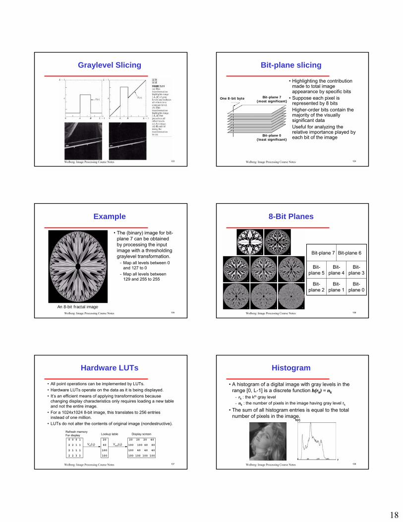
Graylevel Slicing


Bit-plane slicing

• Highlighting the contribution made to total image appearance by specific bits

• Suppose each pixel is represented by 8 bits

• Higher-order bits contain the majority of the visually significant data

• Useful for analyzing the relative importance played by each bit of the image

Bit-plane 7(most significant)

Bit-plane 0(least significant)

One 8-bit byte


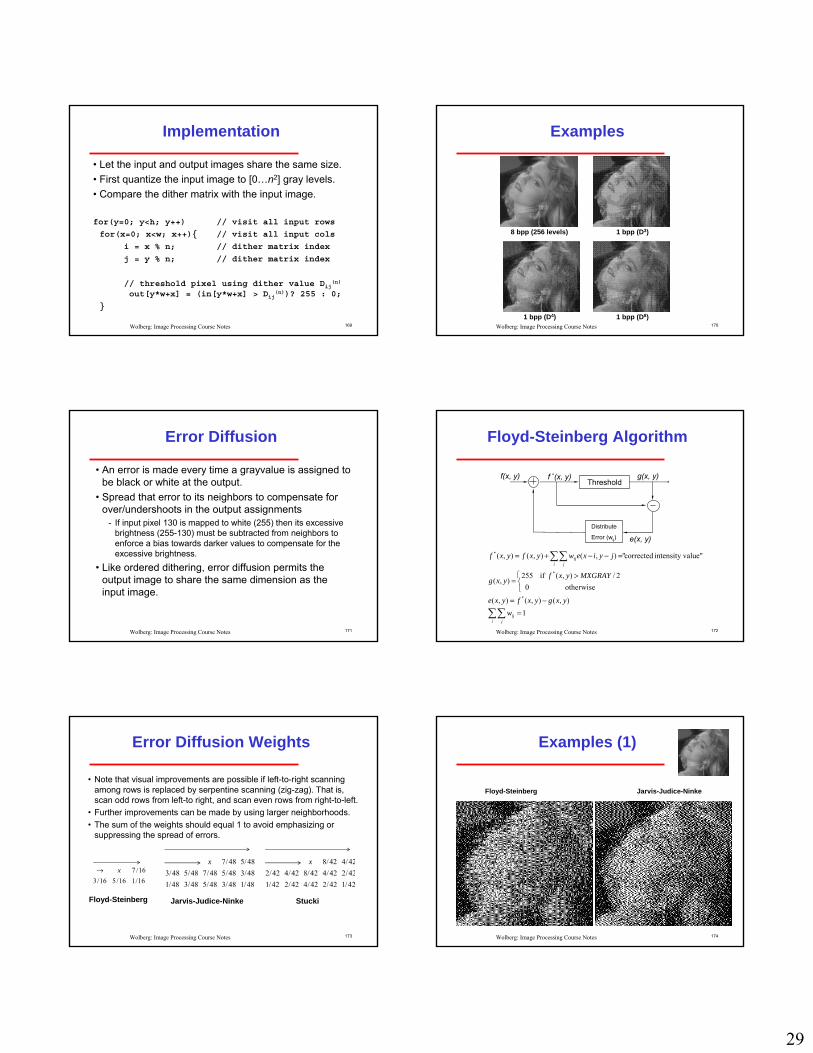
Example

• The (binary) image for bit-plane 7 can be obtained by processing the input image with a thresholding graylevel transformation.

- Map all levels between 0 and 127 to 0

- Map all levels between 129 and 255 to 255

An 8-bit fractal image106Wolberg: Image Processing Course Notes

8-Bit Planes

Bit-plane 6

Bit-plane 0

Bit-plane 1

Bit-plane 2

Bit-plane 3

Bit-plane 4

Bit-plane 5

Bit-plane 7


Hardware LUTs

• All point operations can be implemented by LUTs.• Hardware LUTs operate on the data as it is being displayed.• It’s an efficient means of applying transformations because

changing display characteristics only requires loading a new table and not the entire image.

• For a 1024x1024 8-bit image, this translates to 256 entries instead of one million.

• LUTs do not alter the contents of original image (nondestructive).

0 0 0 1

2 2 1 1

2 1 1 1

2 2 3 3

20

40

100

100

20 20 20 40

100 100 40 40

100 40 40 40

100 100 100 100

Refresh memoryFor display Lookup table Display screen

Vin(i,j) Vout(i,j)


Histogram

• A histogram of a digital image with gray levels in the range [0, L-1] is a discrete function h(rh(rkk) = ) = nnkk

- rk : the kth gray level- nk : the number of pixels in the image having gray level rk

• The sum of all histogram entries is equal to the total number of pixels in the image.

r

h(r)

19


Histogram Example

5x5 image

Histogram evaluation:for(i=0; i<MXGRAY; i++) H[i] = 0;

for(i=0; i<total; i++) H[in[i]]++;

46

25

54

43

32

25Total

51

20

CountGraylevel

2 3 4 4 6

1 2 4 5 6

1 1 5 6 6

0 1 3 3 4

0 1 2 3 4

Plot of the Histogram

0

1

2

3

4

5

6

Pixel value

Cou

nt


Normalized Histogram

• Divide each histogram entry at gray level rrkk by the total number of pixels in the image, nn

p( p( rrkk ) = ) = nnkk / n/ n•• p( p( rrkk )) gives an estimate of the probability of occurrence of gray level rrkk

• The sum of all components of a normalized histogram is equal to 1.


Histogram Processing

•Basic for numerous spatial domain processing techniques.

•Used effectively for image enhancement:- Histogram stretching- Histogram equalization- Histogram matching

• Information inherent in histograms also is useful in image compression and segmentation.


Example: Dark/Bright Images

Dark image

Bright image

Components of histogram are concentrated on the low side of the gray scale.

Components of histogram are concentrated on the high side of the gray scale.


Example: Low/High Contrast Images

Low-contrast image

High-contrast image

histogram is narrow and centered toward the middle of the gray scale

histogram covers broad range of the gray scale and the distribution of pixels is not too far from uniform, with very few vertical lines being much higher than the others


Histogram Stretching

MIN MAX

h(f)

f 0 255

h(g)

g

MINMAXMINfg

−−= )(255

1) Slide histogram down to 0

2) Normalize histogram to [0,1] range

3) Rescale to [0,255] range

20


Example (1)

11 207

Wide dynamic rangepermits for only a smallimprovement after histogramstretching

0 255

Image appears virtuallyidentical to original


Example (2)

• Improve effectiveness of histogram stretching by clipping intensities first

Flat histogram: every graylevelis equally present in image

12811 0 255


Histogram Equalization (1)

• Produce image with flat histogram• All graylevels are equally likely• Appropriate for images with wide range of graylevels• Inappropriate for images with few graylevels (see below)


Histogram Equalization (2)

Objective: we want a uniform histogram. Rationale: maximize image entropy.

This is a special case of histogram matching.Perfectly flat histogram: H[i] = total/MXGRAY for 0≤ i < MXGRAY.If H[v] = k * havg then v must be mapped onto k different levels,

from v1 to vk. This is a one-to many mapping.

avgoutout

avg

out

hvvch

MXGRAYtotalvh

*)1()(

constant)(

1

1

+=

=

==


Histogram Equalization Mappings

Rule 1: Always map v onto (v1+vk)/2. (This does not result in a flat histogram, but one where brightness levels are spaced apart).

Rule 2: Assign at random one of the levels in [v1,vk]. This can result in a loss of contrast if the original histogram had two distinct peaks that were far apart (i.e., an image of text).

Rule 3: Examine neighborhood of pixel, and assign it a level from [v1,vk] which is closest to neighborhood average. This can result in bluriness; more complex.

Rule (1) creates a lookup table beforehand.Rules (2) and (3) are runtime operations.


Example (1)

before after Histogram equalization

21


Example (2)

before after Histogram equalization

The quality is not improved much because the original image already has a wide graylevel scale


Implementation (1)

4242

5323

3424

2332

4x4 image

Gray scale = [0,9]histogram

0 1

1

2

2

3

3

4

4

5

5

6

6

7 8 9

No. of pixels

Gray level


Implementation (2)

9

16/16

16

0

9

s x 9

No. of pixels

Gray Level(j)

99998.4≈8

6.1≈6

3.3≈3

00

16/1616/1616/1616/1615/1611/166/1600

161616161511600

000145600

876543210

∑=

=k

j

j

nn

s0

∑=

k

jjn

0


Implementation (3)

8383

9636

6838

3663

Output image

Gray scale = [0,9]Histogram equalization

0 1

1

2

2

3

3

4

4

5

5

6

6

7 8 9

No. of pixels

Gray level


Note (1)

• Histogram equalization distributes the graylevels to reach maximum gray (white) because the cumulative distribution function equals 1 when 0 ≤ r ≤ L-1

• If is slightly different among consecutive k , those graylevels will be mapped to (nearly) identical values as we have to produce an integer grayvalue as output

• Thus, the discrete transformation function cannot guarantee a one-to-one mapping

∑=

k

jjn

0


Note (2)

• The implementation described above is widely interpreted as histogram equalization.

• It is readily implemented with a LUT.• It does not produce a strictly flat histogram.• There is a more accurate solution. However, it may

require a one-to-many mapping that cannot be implemented with a LUT.

22


Better Implementation (1)

void histeq(imageP I1, imageP I2){

int i, R;int left[MXGRAY], width[MXGRAY];uchar *in, *out;long total, Hsum, Havg, histo[MXGRAY];

/* total number of pixels in image */total = (long) I1->width * I1->height;

/* init I2 dimensions and buffer */I2->width = I1->width;I2->height = I1->height;I2->image = (uchar *) malloc(total);

/* init input and output pointers */in = I1->image; /* input image buffer */out = I2->image; /* output image buffer */

/* compute histogram */for(i=0; i<MXGRAY; i++) histo[i] = 0; /* clear histogram */for(i=0; i<total; i++) histo[in[i]]++; /* eval histogram */R = 0; /* right end of interval */Hsum = 0; /* cumulative value for interval */Havg = total / MXGRAY; /* interval value for uniform histogram */


Better Implementation (2)

/* evaluate remapping of all input gray levels;* Each input gray value maps to an interval of valid output values.* The endpoints of the intervals are left[] and left[]+width[].*/for(i=0; i<MXGRAY; i++) {

left[i] = R; /* left end of interval */Hsum += histo[i]; /* cum. interval value */while(Hsum>Havg && R<MXGRAY-1) { /* make interval wider */

Hsum -= Havg; /* adjust Hsum */R++; /* update right end */

}width[i] = R - left[i] + 1; /* width of interval */

}

/* visit all input pixels and remap intensities */for(i=0; i<total; i++) {

if(width[in[i]] == 1) out[i] = left[in[i]];else { /* in[i] spills over into width[] possible values */

/* randomly pick from 0 to width[i] */R = ((rand()&0x7fff)*width[in[i]])>>15; /* 0 <= R < width */out[i] = left[in[i]] + R;

}}

}


Note

• Histogram equalization has a disadvantage:it can generate only one type of output image.

• With histogram specification we can specify the shape of the histogram that we wish the output image to have.

• It doesn’t have to be a uniform histogram.• Histogram specification is a trial-and-error process.• There are no rules for specifying histograms, and one

must resort to analysis on a case-by-case basis for any given enhancement task.


In the figure above, h() refers to the histogram, and c() refers to its cumulative histogram. Function c() is a monotonically increasing function defined as:

Histogram Matching

vinv’in

C0( v’in)

h0( vin)

vout

C1( v’out)

v’out

C0( vout)

vout=T(vin)

h1( vout)

∫=v

duuhvc0

)()(


Histogram Matching Rule

Let vout =T(vin) If T() is a unique, monotonic function then

This can be restated in terms of the histogram matching rule:

Where c1(vout) = # pixels ≤ vout, and c0(vin) = # pixels ≤ vin..This requires that

which is the basic equation for histogram matching techniques.

∫ ∫=out inv v

duuhduuh0 0

01 )()(

)()( 01 inout vcvc =

))(( 01

1 inout vccv −=


Histograms are Discrete

• Impossible to match all histogram pairs because they are discrete.

1 1 1 1

1 1 2 2

3 3 4 4

4 4 4 4

?

1 1 1 1

2 2 2 2

3 3 3 3

4 4 4 4

Lookup table Display screen

Vin(i,j) Vout(i,j)

Refresh memoryFor display

vinvout vin

C1( vout)

vout

C0( vin) ?

Continuous case Discrete case

23


Problems with Discrete Case

• The set of input pixel values is a discrete set, and all the pixels of a given value are mapped to the same output value. For example, all six pixels of value one are mapped to the same value so it is impossible to have only four corresponding output pixels.

• No inverse for c1 in vout= c1-1(c0(vin)) because of

discrete domain. Solution: choose vout for which c1(vout)is closest to c0(vin).

• vin→ vout such that |c1(vout) - c0(vin)| is a minimum


Histogram Matching Example (1)

Histogram match

Input image

Output image

InputHistogram

TargetHistogram


Histogram Matching Example (2)


Implementation (1)int histogramMatch(imageP I1, imageP histo, imageP I2){

int i, p, R;int left[MXGRAY], right[MXGRAY];int total, Hsum, Havg, h1[MXGRAY], *h2;unsigned char *in, *out;double scale;

/* total number of pixels in image */total = (long) I1->height * I1->width;

/* init I2 dimensions and buffer */I2->width = I1->width;I2->height = I1->height;I2->image = (unsigned char *) malloc(total);

in = I1->image; /* input image buffer */out = I2->image; /* output image buffer */

for(i=0; i<MXGRAY; i++) h1[i] = 0; /* clear histogram */for(i=0; i<total; i++) h1[in[i]]++; /* eval histogram */


Implementation (2)/* target histogram */h2 = (int *) histo->image;

/* normalize h2 to conform with dimensions of I1 */for(i=Havg=0; i<MXGRAY; i++) Havg += h2[i];scale = (double) total / Havg;if(scale != 1) for(i=0; i<MXGRAY; i++) h2[i] *= scale;

R = 0;Hsum = 0;/* evaluate remapping of all input gray levels;

Each input gray value maps to an interval of valid output values.The endpoints of the intervals are left[] and right[] */

for(i=0; i<MXGRAY; i++) {left[i] = R; /* left end of interval */Hsum += h1[i]; /* cumulative value for interval */while(Hsum>h2[R] && R<MXGRAY-1) { /* compute width of interval */

Hsum -= h2[R]; /* adjust Hsum as interval widens */R++; /* update */

}right[i] = R; /* init right end of interval */

}


Implementation (3)

/* clear h1 and reuse it below */for(i=0; i<MXGRAY; i++) h1[i] = 0;

/* visit all input pixels */for(i=0; i<total; i++) {

p = left[in[i]];if(h1[p] < h2[p]) /* mapping satisfies h2 */

out[i] = p;else out[i] = p = left[in[i]] = MIN(p+1, right[in[i]]);h1[p]++;

}}

24


Local Pixel Value Mappings

• Histogram processing methods are global, in the sense that pixels are modified by a transformation function based on the graylevel content of an entire image.

• We sometimes need to enhance details over small areas in an image, which is called a local enhancement.

• Solution: apply transformation functions based on graylevel distribution within pixel neighborhood.


General Procedure

• Define a square or rectangular neighborhood.• Move the center of this area from pixel to pixel.• At each location, the histogram of the points in the

neighborhood is computed and histogram equalization, histogram matching, or other graylevel mapping is performed.

• Exploit easy histogram update since only one new row or column of neighborhood changes during pixel-to-pixel translation.

• Another approach used to reduce computation is to utilize nonoverlapping regions, but this usually produces an undesirable checkerboard effect.


Example: Local Enhancement

a) Original image (slightly blurred to reduce noise)b) global histogram equalization enhances noise & slightly increases

contrast but the structural details are unchangedc) local histogram equalization using 7x7 neighborhood reveals the

small squares inside of the larger ones in the original image.


Definitions (1)

∑

∑

−=

=

ji

ji

yxjifn

yx

jifn

yx

,

2

,

)),(),((1),(

),(1),(

μσ

μ mean

standard deviation

• Let p(ri) denote the normalized histogram entry for grayvalue rifor 0 ≤ i < L where L is the number of graylevels.

• It is an estimate of the probability of occurrence of graylevel ri.• Mean m can be rewritten as

∑−

==

1

0)(

L

iii rprm


Definitions (2)

• The nth moment of r about its mean is defined as

• It follows that:

• The second moment is known as variance • The standard deviation is the square root of the variance.• The mean and standard deviation are measures of

average grayvalue and average contrast, respectively.

)()()(1

0i

L

i

nin rpmrr ∑

−

=

−=μ

)()()(

0)(1)(

21

02

1

0

i

L

ii rpmrr

rr

−=

==

∑−

=

μ

μμ 0th moment

1st moment

2nd moment

)(2 rσ


Example: Statistical Differencing

• Produces the same contrast throughout the image.• Stretch f(x, y) away from or towards the local mean to achieve a balanced

local standard deviation throughout the image.• σ0 is the desired standard deviation and it controls the amount of stretch.• The local mean can also be adjusted:

• m0 is the mean to force locally and α controls the degree to which it is forced.• To avoid problems when σ(x, y) = 0,

• Speedups can be achieved by dividing the image into blocks (tiles), exactly computing the mean and standard deviation at the center of each block, and then linearly interpolating between blocks in order to compute an approximation at any arbitrary position. In addition, the mean and standard deviation can be computed incrementally.

),()),(),((),()1(),( 0

0 yxyxyxfyxmyxg

σσμμαα −+−+=

),()),(),((),()1(),(

0

00 yx

yxyxfyxmyxgβσσβσμμαα

+−+−+=

25


Example: Local Statistics (1)

The filament in the center is clear.There is another filament on the right side that is darker and hard to see. Goal: enhance dark areas while leaving the light areas unchanged.



Solution: Identify candidate pixels to be dark pixels with low contrast.Dark: local mean < k0*global mean, where 0 < k0 < 1.Low contrast: k1*global variance < local variance < k2 * global variance,where k1 < k2.Multiply identified pixels by constant E>1. Leave other pixels alone.



Results for E=4, k0=0.4, k1=0.02, k2=0.4. 3x3 neighborhoods used.

Arithmetic/Logic Operations



Objectives

• In this lecture we describe arithmetic and logic operations commonly used in image processing.

• Arithmetic ops:- Addition, subtraction, multiplication, division- Hybrid: cross-dissolves

• Logic ops:- AND, OR, XOR, BIC, …


Arithmetic/Logic Operations

• Arithmetic/Logic operations are performed on a pixel-by-pixel basis between two images.

• Logic NOT operation performs only on a single image.- It is equivalent to a negative transformation.

• Logic operations treat pixels as binary numbers:- 158 & 235 = 10011110 & 11101011 = 10001010

• Use of LUTs requires 16-bit rather than 8-bit indices:- Concatenate two 8-bit input pixels to form a 16-bit

index into a 64K-entry LUT. Not commonly done.

26


Addition / Subtraction

Addition:for(i=0; i<total; i++)

out[i] = MIN(((int)in1[i]+in2[i]), 255);

Subtraction:for(i=0; i<total; i++)

out[i] = MAX(((int)in1[i]-in2[i]), 0);

in1

in2

+, -, *, ÷ out

Avoid overflow: clip result

Avoid underflow: clip result


Overflow / Underflow

• Default datatype for pixel is unsigned char.• It is 1 byte that accounts for nonnegative range [0,255].• Addition of two such quantities may exceed 255 (overflow).• This will cause wrap-around effect:

- 254: 11111110- 255: 11111111- 256: 100000000- 257: 100000001

• Notice that low-order byte reverts to 0, 1, … when we exceed 255.

• Clipping is performed to prevent wrap-around.• Same comments apply to underflow (result < 0).


Implementation Issues

• The values of a subtraction operation may lie between -255 and 255. Addition: [0,510].

• Clipping prevents over/underflow.• Alternative: scale results in one of two ways:

1. Add 255 to every pixel and then divide by 2.• Values may not cover full [0,255] range• Requires short intermediate image• Fast and simple to implement

2. Add negative of min difference (shift min to 0). Then, multiply all pixels by 255/(max difference) to scale range to [0,255] interval.• Full utilization of [0,255] range• Requires short intermediate image• More complex and difficult to implement


Example of Subtraction Operation


Example: Mask Mode Radiography

• h(x,y) is the mask, an X-ray image of a region of a patient’s body captured by an intensified TV camera (instead of traditional X-ray film) located opposite an X-ray source

• f(x,y) is an X-ray image taken after injection a contrast medium into the patient’s bloodstream

• images are captured at TV rates, so the doctor can see how the medium propagates through the various arteries in an animation of f(x,y)-h(x,y).

mask image h(x,y) image f(x,y) taken after injection of a contrast medium (iodine) into the bloodstream, with mask subtracted out.Note:

• the background is dark because it doesn’t change much in both images.• the difference area is bright because it has a big change


Arithmetic Operations:Cross-Dissolve

• Linearly interpolate between two images.• Used to perform a fade from one image to another.• Morphing can improve upon the results shown below.

for(i=0; i<total; i++)

out[i] = in1[i]*f + in2[i]*(1-f);

0

1

f in1

in2time

in1 in2

27


Masking

• Used for selecting subimages.• Also referred to as region of interest (ROI) processing.• In enhancement, masking is used primarily to isolate

an area for processing.• AND and OR operations are used for masking.


Example of AND/OR Operation

Digital Halftoning



Objectives

• In this lecture we review digital halftoning techniques to convert grayscale images to bitmaps:

- Unordered (random) dithering- Ordered dithering- Patterning- Error diffusion


Background

• An 8-bit grayscale image allows 256 distinct gray levels.• Such images can be displayed on a computer monitor if the

hardware supports the required number of intensity levels.• However, some output devices print or display images with much

fewer gray levels.• In these cases, the grayscale images must be converted to

binary images, where pixels are only black (0) or white (255). • Thresholding is a poor choice due to objectionable artifacts.• Strategy: sprinkle black-and-white dots to simulate gray.• Exploit spatial integration (averaging) performed by eye.


Thresholding

• The simplest way to convert from grayscale to binary.

0 255 vinthr

vout

8 bpp (256 levels) 1 bpp (two-level)

Loss of information is unacceptable.

28


Unordered Dither (1)

• Reduce quantization error by adding uniformly distributed white noise (dither signal) to the input image prior to quantization.

• Dither hides objectional artifacts.• To each pixel of the image, add a random number in the range [-m,

m], where m is MXGRAY/quantization-levels.

0 255 vinthr

vout

8 bpp (256 levels)

Uniformnoise

3 bpp (8 levels)


Unordered Dither (2)

1 bpp

Quantization

Dither/Quantization

2 bpp 3 bpp 4 bpp


Ordered Dithering

• Objective: expand the range of available intensities. • Simulates n bpp images with m bpp, where n>m (usually m = 1).• Exploit eye’s spatial integration.

- Gray is due to average of black/white dot patterns.- Each dot is a circle of black ink whose area is proportional to ( 1 – intensity).- Graphics output devices approximate the variable circles of halftone

reproductions.

• 2 x 2 pixel area of a bilevel display produces 5 intensity levels.• n x n group of bilevel pixels produces n2+1 intensity levels.• Tradeoff: spatial vs. intensity resolution.

0 1 2 3 4


Dither Matrix (1)

• Consider the following 2x2 and 3x3 dither matrices:

• To display a pixel of intensity I, we turn on all pixels whose associated dither matrix values are less than I.

• The recurrence relation given below generates larger dither matrices of dimension n x n, where n is a power of 2.

where U(n) is an n x n matrix of 1’s.

⎥⎥⎥

⎦

⎤

⎢⎢⎢

⎣

⎡=⎥

⎦

⎤⎢⎣

⎡=

725301486

1320 )3()2( DD

⎥⎦

⎤⎢⎣

⎡

++++

= )2/()2(11

)2/()2/()2(10

)2/(

)2/()2(01

)2/()2/()2(00

)2/()(

4444

nnnn

nnnnn

UDDUDDUDDUDD

D


• Example: a 4x4 dither matrix can be derived from the 2x2 matrix.

Dither Matrix (2)

⎥⎥⎥⎥

⎦

⎤

⎢⎢⎢⎢

⎣

⎡

=

51371591113614412

10280

)4(D

13 14 15 16

9

5

1 2 3 4

12

8


Patterning

• Let the output image be larger than the input image.• Quantize the input image to [0…n2] gray levels.• Threshold each pixel against all entries in the dither matrix.

- Each pixel forms a 4x4 block of black-and-white dots for a D(4) matrix.- An n x n input image becomes a 4n x 4n output image.

• Multiple display pixels per input pixel.• The dither matrix Dij

(n) is used as a spatially-varying threshold.• Large input areas of constant value are displayed exactly as before.

nn

4n

4n

29


Implementation

• Let the input and output images share the same size.• First quantize the input image to [0…n2] gray levels.• Compare the dither matrix with the input image.

for(y=0; y<h; y++) // visit all input rows

for(x=0; x<w; x++){ // visit all input cols

i = x % n; // dither matrix index

j = y % n; // dither matrix index

// threshold pixel using dither value Dij(n)

out[y*w+x] = (in[y*w+x] > Dij(n))? 255 : 0;

}


Examples

1 bpp (D4)

8 bpp (256 levels) 1 bpp (D3)

1 bpp (D8)


Error Diffusion

• An error is made every time a grayvalue is assigned to be black or white at the output.

• Spread that error to its neighbors to compensate for over/undershoots in the output assignments

- If input pixel 130 is mapped to white (255) then its excessive brightness (255-130) must be subtracted from neighbors to enforce a bias towards darker values to compensate for the excessive brightness.

• Like ordered dithering, error diffusion permits the output image to share the same dimension as the input image.


Floyd-Steinberg Algorithm

Threshold

Distribute

Error (wij)

f(x, y) f *(x, y) g(x, y)

e(x, y)

∑∑

∑∑

=−=

⎩⎨⎧ >

=

=−−+=

i jij

i jij

wyxgyxfyxe

MXGRAYyxfyxg

jyixewyxfyxf

1),(),(),(

otherwise02/),( if255

),(

value"intensity corrected"),(),(),(

*

*

*


Error Diffusion Weights

• Note that visual improvements are possible if left-to-right scanning among rows is replaced by serpentine scanning (zig-zag). That is, scan odd rows from left-to right, and scan even rows from right-to-left.

• Further improvements can be made by using larger neighborhoods.• The sum of the weights should equal 1 to avoid emphasizing or

suppressing the spread of errors.

16/116/516/316/7x→

Floyd-Steinberg

48/148/348/548/348/148/348/548/748/548/348/548/7x

Jarvis-Judice-Ninke

42/142/242/442/242/142/242/442/842/442/242/442/8x

Stucki


Examples (1)

Floyd-Steinberg Jarvis-Judice-Ninke

30


Examples (2)



Examples (3)



Implementationthr = MXGRAY /2; // init threshold valuefor(y=0; y<h; y++){ // visit all input rowsfor(x=0; x<w; x++) { // visit all input cols

*out = (*in < thr)? // thresholdBLACK : WHITE; // note: use LUT!

e = *in - *out; // eval errorin[ 1 ] +=(e*7/16.); // add error to E nbrin[w-1] +=(e*3/16.); // add error to SW nbrin[ w ] +=(e*5/16.); // add error to S nbrin[w+1] +=(e*1/16.); // add error to SE nbr

in++; // advance input ptrout++; // advance output ptr

}}


Comments

• Two potential problems complicate implementation:- errors can be deposited beyond image border- errors may force pixel grayvalues outside the [0,255] range

True for allneighborhood ops

16/116/516/316/7x→

Floyd-Steinberg

Right border

Bottom border

48/148/348/548/348/148/348/548/748/548/348/548/7x

Jarvis-Judice-Ninke

Right border


Solutions to Border Problem (1)

• Perform if statement prior to every error deposit- Drawback: inefficient / slow

• Limit excursions of sliding weights to lie no closer than 1 pixel from image boundary (2 pixels for J-J-N weights).

- Drawback: output will be smaller than input• Pad image with extra rows and columns so that limited

excursions will yield smaller image that conforms with original input dimensions. Padding serves as placeholder.

- Drawback: excessive memory needs for intermediate image

input padded input output180Wolberg: Image Processing Course Notes

Solutions to Border Problem (2)

• Use of padding is further undermined by fact that 16-bit precision (short) is needed to accommodate pixel values outside [0, 255] range.

• A better solution is suggested by fact that only two rows are active while processing a single scanline in the Floyd-Steinberg algorithm (3 for JJN).

• Therefore, use a 2-row (or 3-row) circular buffer to handle the two (or three) current rows.

• The circular buffer will have the necessary padding and 16-bit precision.

• This significantly reduces memory requirements.

31


Circular Buffer

01

21

23

34

012345

input circular buffer(snapshots)

012345

output


New Implementationthr = MXGRAY /2; // init threshold valuecopyRowToCircBuffer(0); // copy row 0 to circular bufferfor(y=0; y<h; y++){ // visit all input rowscopyRowToCircBuffer(y+1); // copy next row to circ bufferin1 = buf[ y %2] + 1; // circ buffer ptr; skip over padin2 = buf[(y+1)%2] + 1; // circ buffer ptr; skip over padfor(x=0; x<w; x++) { // visit all input cols

*out = (*in1 < thr)? BLACK : WHITE; // threshold

e = *in1 - *out; // eval errorin1[ 1] +=(e*7/16.); // add error to E nbrin2[-1] +=(e*3/16.); // add error to SW nbrin2[ 0] +=(e*5/16.); // add error to S nbrin2[ 1] +=(e*1/16.); // add error to SE nbr

in1++; in2++ // advance circ buffer ptrsout++; // advance output ptr

}}

Neighborhood Operations



Objectives

• This lecture describes various neighborhood operations:

- Blurring- Edge detection- Image sharpening- Convolution


Neighborhood Operations

• Output pixels are a function of several input pixels.• h(x,y) is defined to weigh the contributions of each

input pixel to a particular output pixel.• g(x,y) = T[f(x,y); h(x,y)]


Filterh(x,y)

g(x,y)=T[f(x,y); h(x,y)]=f(x,y)*h(x,y)


Spatial Filtering

• h(x,y) is known as a filter kernel, filter mask, or window.• The values in a filter kernel are coefficients.• Kernels are usually of odd size: 3x3, 5x5, 7x7• This permits them to be properly centered on a pixel

- Consider a horizontal cross-section of the kernel.- Size of cross-section is odd since there are 2n+1 coefficients: n

neighbors to the left + n neighbors to the right + center pixel

h1 h3h2

h5h4

h8

h6

h9h7

32


Spatial Filtering Process

• Slide filter kernel from pixel to pixel across an image.• Use raster order: left-to-right from the top to the bottom.• Let pixels have grayvalues fi.• The response of the filter at each (x,y) point is:

∑=

=

+++=mn

iiii

mnmn

fh

fhfhfhR ...2211

Σhij

549538527

446435424

34333232143

(4,3)at centered Window

fhfhfhfhfhfhfhfhfhg

++++++++=Kernel slides

across imageIn raster order

1D indexing

2D indexing


Linear Filtering

• Let f(x,y) be an image of size MxN.• Let h(i,j) be a filter kernel of size mxn.• Linear filtering is given by the expression:

• For a complete filtered image this equation must be applied for x = 0, 1, 2, … , M-1 and y = 0, 1, 2, … , N-1.

∑ ∑−= −=

++=s

si

t

tj

jyixfjihyxg ),(),(),(

where s = (m-1)/2 and t = (n-1)/2


Spatial Averaging

• Used for blurring and for noise reduction• Blurring is used in preprocessing steps, such as

- removal of small details from an image prior to object extraction- bridging of small gaps in lines or curves

• Output is average of neighborhood pixels.• This reduces the “sharp” transitions in gray levels.• Sharp transitions include:

- random noise in the image- edges of objects in the image

• Smoothing reduces noise (good) and blurs edges (bad)


3x3 Smoothing Filters

• The constant multiplier in front of each kernel is equal to the sum of the values of its coefficients.

• This is required to compute an average.

The center is the most important and other pixels are inversely weighted as a function of their distance from the center of the mask. This reduces blurring in the smoothing process.

Box filter Weighted average


• Unweighted averaging (smoothing filter):

• Weighted averaging:

Unweighted/Weighted Averaging

∑=ji

jifm

yxg,

),(1),(

∑ −−=ji

jyixhjifyxg,

),(),(),(

7x7 unweighted averagingOriginal image 7x7 Gaussian filter


Unweighted Averaging

• Unweighted averaging over a 5-pixel neighborhood along a horizontal scanline can be done with the following statement:for(x=2; x<w-2; x++)

out[x]=(in[x-2]+in[x-1]+in[x]+in[x+1]+in[x+2])/5;

• Each output pixel requires 5 pixel accesses, 4 adds, and 1 division. A simpler version (for unweighted averaging only) is:sum=in[0]+in[1]+in[2]+in[3]+in[4];

for(x=2; x<w-2; x++){

out[x] = sum/5;

sum+=(in[x+3] – in[x-2]);

}

Limited excursions reduce size of output

-

+

33


Image Averaging

• Consider a noisy image g(x,y) formed by the addition of noise η(x,y) to an original image f(x,y):

g(x,y) = f(x,y) + η(x,y)• If the noise has zero mean and is uncorrelated then we can

compute the image formed by averaging K different noisy images:

• The variance of the averaged image diminishes:

• Thus, as K increases the variability (noise) of the pixel at each location (x,y) decreases assuming that the images are all registered (aligned).

∑=

=K

ii yxg

Kyxg

1),(1),(

),(2

),(2 1

yxyxgK

ησσ =


Noise Reduction (1)

• Astronomy is an important application of image averaging.

• Low light levels cause sensor noise to render single images virtually useless for analysis.


Noise Reduction (2)

• Difference images and their histograms yield better appreciation of noise reduction.

• Notice that the mean and standard deviation of the difference images decrease as K increases.


General Form: Smoothing Mask

• Filter of size mxn (where m and n are odd)

∑ ∑

∑ ∑

−= −=

−= −=

++= s

si

t

tj

s

si

t

tj

jih

jyixfjihyxg

),(

),(),(),(

summation of all coefficients of the mask

Note that s = (m-1)/2 and t = (n-1)/2


Example

• a) original image 500x500 pixel• b) - f) results of smoothing with

square averaging filter of size n = 3, 5, 9, 15 and 35, respectively.

• Note:- big mask is used to eliminate small

objects from an image.- the size of the mask establishes the

relative size of the objects that will be blended with the background.

fedcba


Example

• Blur to get gross representation of objects.• Intensity of smaller objects blend with background.• Larger objects become blob-like and easy to detect.

original image result after smoothingwith 15x15 filter

result of thresholding

34


Unsharp Masking

• Smoothing affects transition regions where grayvalues vary.• Subtraction isolates these edge regions.• Adding edges back onto image causes edges to appear more

pronounced, giving the effect of image sharpening.

Blur - +

Edge image

Sharpen image


Order-Statistics Filters

• Nonlinear filters whose response is based on ordering (ranking) the pixels contained in the filter support.

• Replace value of the center pixel with value determined by ranking result.

• Order statistic filters applied to nxn neighborhoods:- median filter: R = median{zk |k = 1,2,…,n2}- max filter: R = max{zk |k = 1,2,…, n2}- min filter: R = min{zk |k = 1,2,…, n2}


Median Filter

• Sort all neighborhood pixels in increasing order.• Replace neighborhood center with the median.• The window shape does not need to be a square.• Special shapes can preserve line structures.• Useful in eliminating intensity spikes: salt & pepper noise.

252025

1520020

202010 (10,15,20,20,20,20,20,25,200)Median = 20Replace 200 with 20


Median Filter Properties

• Excellent noise reduction • Forces noisy (distinct) pixels to conform to their neighbors.• Clusters of pixels that are light or dark with respect to their

neighbors, and whose area is less than n2/2 (one-half the filter area), are eliminated by an n x n median filter.

• k-nearest neighbor is a variation that blends median filtering with blurring:

- Set output to average of k nearest entries around median

252025

1520020

191810 (10,15,18,19,20,20,20,25,200)k=1: replace 200 with (19+20+20)/3k=2: replace 200 with (18+19+20+20+20)/5k=3: replace 200 with (15+18+19+20+20+20+25)/7k=4: replace 200 with (10+15+18+19+20+20+20+25+200)/9


Examples (1)

Additive salt & pepper noise Median filter output Blurring output

204

Examples (2)

35

205

Derivative Operators

• The response of a derivative operator is proportional to the degree of discontinuity of the image at the point at which the operator is applied.

• Image differentiation- enhances edges and other discontinuities (noise)- deemphasizes area with slowly varying graylevel values.

• Derivatives of a digital function are approximated by differences.


First-Order Derivative

• Must be zero in areas of constant grayvalues.• Must be nonzero at the onset of a grayvalue step or ramp.• Must be nonzero along ramps.

)()1()( xfxfxxf −+=

∂∂


Second-Order Derivative

• Must be zero in areas of constant grayvalues.• Must be nonzero at the onset of a grayvalue step or ramp.• Must be zero along ramps of constant slope.

)(2)1()1(

)1()()(2

2

xfxfxf

xfxfx

xf

−−++=

−∂−∂=∂

∂


Example


Comparisons

• 1st-order derivatives:- produce thicker edges- strong response to graylevel steps

• 2nd-order derivatives:- strong response to fine detail (thin lines, isolated points)- double response at step changes in graylevel


Laplacian Operator

• Simplest isotropic derivative operator• Response independent of direction of the discontinuities.• Rotation-invariant: rotating the image and then applying

the filter gives the same result as applying the filter to the image first and then rotating the result.

• Since derivatives of any order are linear operations, the Laplacian is a linear operator.

2

2

2

22

yf

xff

∂∂+

∂∂=∇

36


Discrete Form of Laplacian

),(2),1(),1(2

2

yxfyxfyxfx

f −−++=∂∂

),(2)1,()1,(2

2

yxfyxfyxfy

f −−++=∂∂

)],(4)1,()1,(),1(),1([2

yxfyxfyxfyxfyxff−−+++

−++=∇

2

2

2

22

yf

xff

∂∂+

∂∂=∇

where


Laplacian MaskIsotropic resultfor rotations inincrements of 90°

Isotropic resultfor rotations inincrements of 45°


Another Derivation

In constant areas: 0Near edges: high values

111

111

111

1/9* Unweighted Average Smoothing Filter

000

010

000Retain Original

-1-1-1

-18-1

-1-1-1

1/9* Original – Average (negative of Laplacian Operator)

Summation of coefficients in masks equals 0.


Effect of Laplacian Operator

• Since the Laplacian is a derivative operator- it highlights graylevel discontinuities in an image- it deemphasizes regions with slowly varying gray levels

• The Laplacian tends to produce images that have- grayish edge lines and other discontinuities all superimposed

on a dark featureless background


Example

-1-1-1

-18-1

-1-1-1


Simplification

• Addition of image with Laplacian can be combined into one operator:

)]1,()1,( ),1(),1([),(5)],(4)1,()1,(

),1(),1([),(),(

−+++−++−=

+−+++−++−=

yxfyxfyxfyxfyxfyxfyxfyxf

yxfyxfyxfyxg

0-10

-15-1

0-10

000

010

000

= +0-10

-14-1

0-10

37


Example


Gradient Operator (1)

• The gradient is a vector of directional derivatives.

• Although not strictly correct, the magnitude of the gradient vector is referred to as the gradient.

• First derivatives are implemented using this magnitude

⎥⎥⎥⎥

⎦

⎤

⎢⎢⎢⎢

⎣

⎡

∂∂∂∂

=⎥⎦

⎤⎢⎣

⎡=∇

yfxf

ff

y

xf

21

22

2122 ][

)(mag

⎥⎥⎦

⎤

⎢⎢⎣

⎡⎟⎟⎠

⎞⎜⎜⎝

⎛∂∂+⎟

⎠⎞

⎜⎝⎛∂∂=

+=

∇=∇

yf

xf

ff

f

yx

f

yx fff +≈∇

approximation:


Gradient Operator (2)

• The components of the gradient vector are linear operators, but the magnitude is not (square,square root).

• The partial derivatives are not rotation invariant (isotropic), but the magnitude is.

• The Laplacian operator yields a scalar: a single number indicating edge strength at point.

• The gradient is actually a vector from which we can compute edge magnitude and direction.

x

yangle

yxmagyxmag

ff

jif

ffjifffjif

1

22

tan),(

),(or ),(

−=

+=+=

)1,()1,(),(),1(),1(),(

−−+=−−+=jifjifjif

jifjifjif

y

xwhere


Summary (1)

[ ] [ ]

( )( )( )( ))1()()1(121

)()1()2(121 )()1(2)2(

)2()1()1()( )1()()( )()(

)1()()( )( )(

Digital Continuous

''''2''

''

+−−=−−−=

+−−−=−−−−−−=

−−=∇=

−−=

iviviviviviv

iviviviviviviv

ivivivxfxfivivivxf

v(i)xf

-1-1-1

-18-1

-1-1-1

-1

-14-1

-1

The Laplacian is a scalar, giving only the magnitude about the change in pixel values at a point. The gradient gives both magnitude and direction.


Summary (2)

[ ]

⎥⎥⎥

⎦

⎤

⎢⎢⎢

⎣

⎡−=

−=

101

mask

101mask:ldimensiona One

y

x

⎥⎥⎥

⎦

⎤

⎢⎢⎢

⎣

⎡ −−−=

⎥⎥⎥

⎦

⎤

⎢⎢⎢

⎣

⎡

−−−

=

⎥⎥⎥

⎦

⎤

⎢⎢⎢

⎣

⎡ −−−=

⎥⎥⎥

⎦

⎤

⎢⎢⎢

⎣

⎡

−−−

=

111000111

mask 101101101

mask

:OperatorPrewitt 121000121

mask 101202101

mask

:Operator Sobel:ldimensiona Two

yx

yx

x

yangle

yxmagyxmag

ff

jif

ffjifffjif

1

22

tan),(

),(or ),(

−=

+=+= in Gradient

Mag

Angle

in Laplacian Mag


Example (1)

38


Example (2)

• Goal: sharpen image and bring out more skeletal detail.• Problem: narrow dynamic range and high noise content

makes the image difficult to enhance.• Solution:

1. Apply Laplacian operator to highlight fine detail2. Apply gradient operator to enhance prominent edges3. Apply graylevel transformation to increase dynamic range



Filtering Theory



Objectives

• This lecture reviews filtering theory.- Linearity and spatial-invariance (LSI)- Impulse response- Sifting integral- Convolution


• We use two criteria for filters: linearity and spatial-invariance

Definitions

f(x) Filter g(x) f(x) g(x)

)()(

)()()()(simply,or

ionsuperposit )()()()(input toalproportion isoutput )()(

2121

2121

λλ

βαβα

αα

−→−

+→+

+→+→

xgxf

xgxgxfxf

xgxgxfxfxgxf

:invariant)-shiftinvariant(-Space

:Linear

39


• Physically realizable filters (lenses) are rarely LSI filters.- Optical systems impose a limit in their maximum response.- Power can’t be negative, imposing a limit on the minimum response.- Lens aberrations and finite image area prevent LSI property.

• Nevertheless, close enough to approximate as LSI.

LSI Filter


Impulse Response

δ(x) Filter h(x)

⎪⎩

⎪⎨⎧

≠

=== ∫−

→

0 ,0

0 ,1)(lim)(''

0

x

xdxxfx

ε

εεδ

0 x 0 xα

δ(x) Spike at x=0 δ(x- α)

δ(x) is the impulse function, or Dirac delta function which is a continuous function.

∫

∫

∞

∞−

∞

∞−

−=

⎩⎨⎧

≠=

=

−−=

λλδλ

δ

λδλλδλ

dxfxf

xx

x

xxfxdxfxf

)()()(

0 ,00 ,1

)(

at )( samples )( )()()( 0000

Kronecker delta function (discrete case: integer values of x)

Sifting integral


Convolution

• Any input signal can be represented by an infinite sum of shifted and scaled impulses:

Convolution:

Input

0 x

δ(x)

Filter

0

h(x)

outputBlurred version of input

∫∞

∞−−== λλλ dxhfxhxfxg )()()(*)()( :continuous


Discrete Case

• Input function is a scaled shifted version of impulse response.⊗, *: convolution operatorh(x): convolution kernel, filter kernel

• If h(x) = δ(x) then we have an ideal filter: output = input.• Usually h(x) extends over several neighbors.• Discrete convolution:

∑∞

∞−

−=⊗= )()()()()( λλ xhfxhxfxg


Example: Triangle Filter

• Linearity rule: scale h(x) according to f(x) and add g1, g2.• Obtain f(x) for any x by sampling the reconstructed g(x).

⎩⎨⎧

≤<≤−

=x

xxxh

1 010 1

)(-1 1

1

0 x

0 1g1

g2

gf1

f2

x11221

2211

)(gg1x0 )1(

fxffgxfgxfg+−=+=

≤≤=−=

Input samples (impulses) Impulse responses (additive)

Addition of two adjacent impulse responses Straight line: y=mx+b


Convolution Summation

• g(x) is a continuous convolution summation to compute at particular values at x.

∑∞

∞−

−=⊗= )()()()()( λλ xhfxhxfxg

f1

f2

x1 x2x

g(x) = f1h(x-x1) + f2h(x-x2)If x1=0 and x2=1 then g(x)=f1(1-x)+f2x

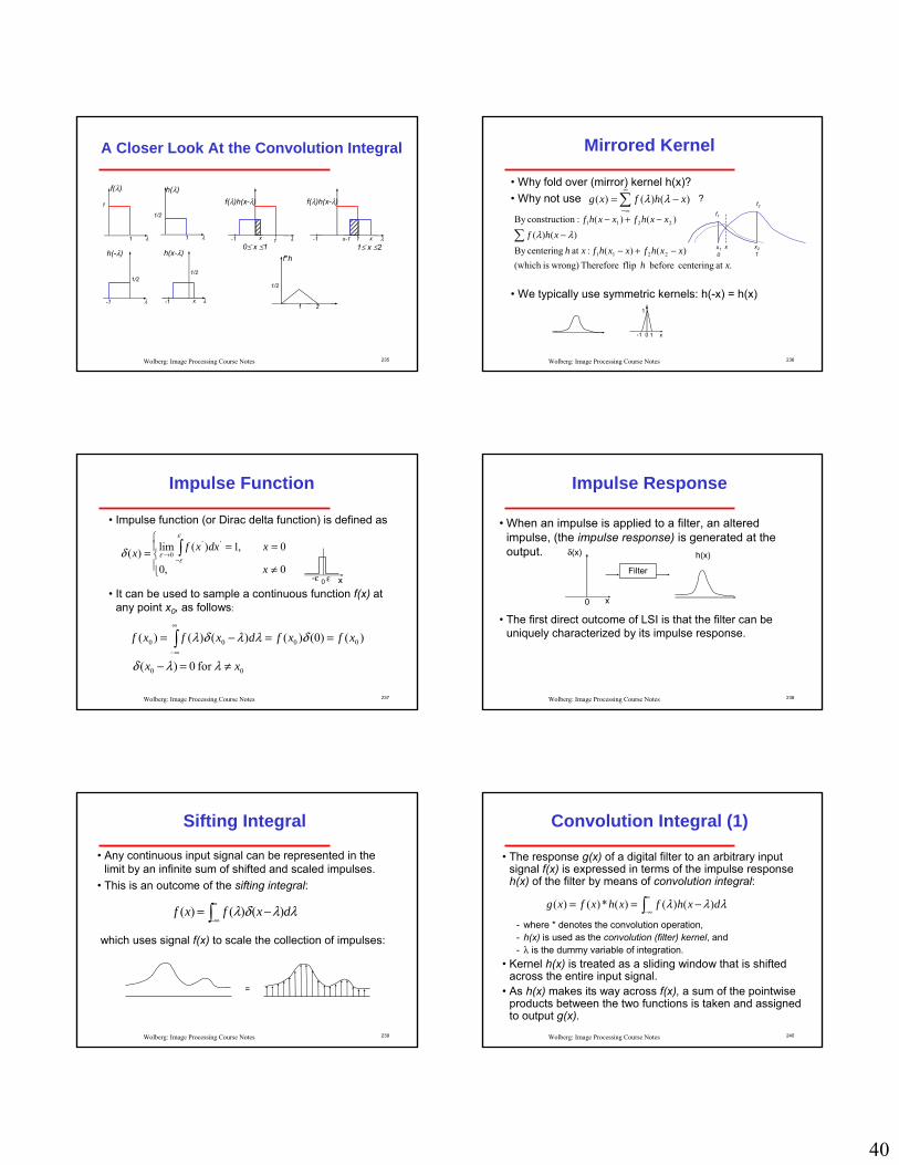
40


A Closer Look At the Convolution Integral

f(λ)

1 λ 1 λ

h(λ)

1

1/2

-1 λ

h(-λ)

1/2

-1 λ

h(x-λ)

1/2

x

-1 λ

f(λ)h(x-λ)

x 10≤ x ≤1

-1 λ

f(λ)h(x-λ)

x11≤ x ≤2

x-1

1 2

1/2

f*h


Mirrored Kernel

• Why fold over (mirror) kernel h(x)?• Why not use

• We typically use symmetric kernels: h(-x) = h(x)

∑∞

∞−−= )()()( xhfxg λλ f2

f1

x1 x2x0 1

.at centering before flip Therefore wrong)is(which )()( :at centeringBy

)()()()(:onconstructiBy

2211

2211

xhxxhfxxhfxh

xhfxxhfxxhf

−+−

−−+−

∑ λλ

-1 1

1

0 x

?


Impulse Function

• Impulse function (or Dirac delta function) is defined as

• It can be used to sample a continuous function f(x) at any point x0, as follows:

⎪⎩

⎪⎨⎧

≠

=== ∫−

→

0 ,0

0 ,1)(lim)(''

0

x

xdxxfx

ε

εεδ

0 xε-ε

00

0000

for 0 )(

)( (0))()()()(

xx

xfxfdxfxf

≠=−

==−= ∫∞

∞−

λλδ

δλλδλ


Impulse Response

• When an impulse is applied to a filter, an altered impulse, (the impulse response) is generated at the output.

• The first direct outcome of LSI is that the filter can be uniquely characterized by its impulse response.

0 x

δ(x)

Filter

h(x)


Sifting Integral

• Any continuous input signal can be represented in the limit by an infinite sum of shifted and scaled impulses.

• This is an outcome of the sifting integral:

which uses signal f(x) to scale the collection of impulses:

∫∞

∞−−= λλδλ dxfxf )()()(

=


Convolution Integral (1)

• The response g(x) of a digital filter to an arbitrary input signal f(x) is expressed in terms of the impulse response h(x) of the filter by means of convolution integral:

- where * denotes the convolution operation,- h(x) is used as the convolution (filter) kernel, and - λ is the dummy variable of integration.

• Kernel h(x) is treated as a sliding window that is shifted across the entire input signal.

• As h(x) makes its way across f(x), a sum of the pointwiseproducts between the two functions is taken and assigned to output g(x).

∫∞

∞−−== λλλ dxhfxhxfxg )()()(*)()(

41


Convolution Integral (2)

• This process, known as convolution, is of fundamental importance to linear filtering theory.

• It simply states that the output of an LSI filter will be a superposition of shifted and scaled impulse responses.

• This is used to explain how a continuous image is blurred by a camera as it passes through the lens.

- In this context, h(x) is known as the point spread function (PSF), reflecting the limitation of the camera to accurately resolve a small point without somewhat blurring it.

outputFilter


Evaluation

• We can arrive at g(x) in two ways:- Graphical construction of a series of shifted/scaled impulse responses- Computing the convolution summation at all points of interest

• Graphical construction more closely follows the physical process as an input signal passes through a filter.

• Convolution summation more closely follows the practical evaluation of g(x) at a finite number of desired points.

- instead of adding scaled and shifted unit impulse responses (responses of unit impulses), we center the unit impulse response at the point of interest.


Graphical Construction

0 x

δ(x)

Filter

h(x)

0-1-2 1 2

.51 Asymmetric unit impulse response

with an extent of 5 points

0-1-2 1 2 3 4 5

1

2

11.5

g(x0)

x0

Filterf1=2

f2=4

f3=2

f4=3

0 1 2 3

)3(3)2(2)1(4)(2)()3()2()1()()(

00000

040302010

−+−+−+=−+−+−+=

xhxhxhxhxgxhfxhfxhfxhfxg

0 1 2

1

2

1

1.5

g(x0)

x0

B

A

DC

Blowup ofintervalbetween1 and 2

As we scan fi from left to right we multiply samples with values taken from hin right to left order.

.5

h(x0)

h(x0-1)

h(x0-2)

h(x0-3)

x0-1x0-2x0-3 x0


Convolution Summation (1)

• Instead of adding scaled/shifted unit impulse responses, center unit impulse response at point of interest:

• As λ increases, we scan f() from left to right. However, h(x0- λ) is scanned from right to left.

• Reason: points to the left of x0 had contributed to x0 through the right side of h (see graphical construction).

f1=2

f2=4

f3=2

f4=3

0 1 2 3

.5∫∞

∞−−= λλλ dxhfxg )()()( 00

x0

h(x0-λ)



• More straightforward: implement convolution if both the input and the kernel were scanned in the same direction.

• This permits direct pointwise multiplication among them.• Thus, flip kernel before centering it on output position.

f1=2

f2=4

f3=2

f4=3

0 1 2 3

.5

x0x1 x2 x3 x4

h1

h2

h3

h4



• will yield the value for g(x0), where hi = h(xi-x0).• Rationale: multiplying the unit impulse response h with fi,

h is being scaled. The distance between x0 and xiaccounts for the effect of a shifted response function on the current output.

• For most impulse response functions, h will taper off with increasing distance from its center.

• If the kernel is symmetric (h(x)=h(-x)), it is not necessary to flip the kernel before centering.

∑=

4

1iiihf

42


• The kernel is often a discrete set of weights, i.e., a 3x3 filter kernel.• As long as kernel is shifted in pixel (integer) increments across the

image, there is no alignment problem with underlying image.• However, for noninteger pixel increments the kernel values may have

no corresponding image values.

Discrete Convolution (1)

∑∞

∞−

−= )()()( λλ xhfxg

f5

f1f2

f3f4

h-2h-1

h0 h1 h2

h-2h-1 h1 h2

h0

h is aligned with f(h is centered at pixel f3)

h is not aligned with fIt has been shifted by a½-pixel increment

for integer values of λ and arbitrary values of x


Discrete Convolution (2)

There are two possible solutions to this problem:1. Represent h in analytic form for evaluation anywhere

Ex: Let bell-shape PSF be h(x)=2-4x2. The appropriate weight to apply to fi can be obtained by setting x to the difference between the center of the bell (impulse response) and the position of the fi.

2. Supersample h so that a dense set of samples are used to represent h. The supersampled version will then be aligned with the image data, or at least it will have values that are nearby.

f1f2

f3f4

f5

Supersampled kernel

Closest kernel samples from supersampled set

If the kernel is known to be slid across theimage at fixed increments, then the kernelcan be sampled at known positions.Ex: a 1/3 increment requires the kernel toBe sampled three times per unit interval.

Fourier Transform



Objectives

• This lecture reviews Fourier transforms and processing in the frequency domain.

- Definitions- Fourier series- Fourier transform- Fourier analysis and synthesis- Discrete Fourier transform (DFT)- Fast Fourier transform (FFT)


Background (1)

• Fourier proved that any periodic function can be expressed as the sum of sinusoids of different frequencies, each multiplied by a different coefficient. → Fourier series

• Even aperiodic functions (whose area under the curve isfinite) can be expressed as the integral of sinusoidsmultiplied by a weighting function. → Fourier transform

• In a great leap of imagination, Fourier outlined these results in a memoir in 1807 and published them in La TheorieAnalitique de la Chaleur (The Analytic theory of Heat) in 1822. The book was translated into English in 1878.


Background (2)

• The Fourier transform is more useful than the Fourier series in most practical problems since it handles signals of finite duration.

• The Fourier transform takes us between the spatial and frequency domains.

• It permits for a dual representation of a signal that is amenable for filtering and analysis.

• Revolutionized the field of signal processing.

43


Example


Useful Analogy

• A glass prism is a physical device that separates light into various color components, each depending on its wavelength (or frequency) content.

• The Fourier transform is a mathematical prism that separates a function into its frequency components.


Fourier Series forPeriodic Functions


Fourier Transform forAperiodic Functions


Fourier Analysis and Synthesis

• Fourier analysis: determine amplitude & phase shifts• Fourier synthesis: add scaled and shifted sinusoids together• Fourier transform pair:

uuxiuxi

dxeuFxf

dxexfuF

ux

uxi

uxi

freq.at lexponentiacomplex )2sin()2cos(eand ,1 where

)()( F.T. Inverse

)()( F.T. Forward

i2

2

2

←±=−=

=

=

±

∞

∞−

+

∞

∞−

−

∫

∫

πππ

π

π

Euler’s formula


Fourier Coefficients

• Fourier coefficients F(u) specify, for each frequency u, the amplitude and phase of each complex exponential.

• F(u) is the frequency spectrum.• f(x) and F(u) are two equivalent representations of the

same signal.

spectrum phase )()(tan)(

spectrumFourier aka spectrum; magnitude )()()(

)()()(

1

22

←=Φ

←+=

+=

−

uRuIu

uIuRuF

uiIuRuF

density spectral )()(|)(|)(

22

2

←+=

=

uIuRuFuP

44


1D Example

W

A

x ⎩⎨⎧

>≤≤

=Wx

WxAxf

00

)(

∫ ∫∞

∞−

− == axaxuxi ea

dxedxexfuF 1 :note )()( 2π

[ ] [ ]

( )

( ) ( ) ( )

))sin(sinc ( )sin(sinc where

sinsinsin)(

sin)(

2sin :note ][

2)(

]1[2

122

)(

)(

220

2

0

2

xx(x)havebookssome

xx(x)

uWcAWuW

uWAWeuWuAuF

nctioncomplex fueuWuAuF

ieexeee

uiAuF

eui

Aeui

Aeui

AuF

dxAeuF

uWi

uWi

ixixuwiuwiuwi

uwiuwiWuxi

Wuxi

==

===

←=

−=−=

−=−−=−=

=

−

−

−−−

−−−

−∫

ππ

ππππ

π

ππ

π

πππ

π

π

πππ

πππ

π

AW

01/w

2/w3/w-3/w

-2/w-1/w u

1

0 2 4-4 -2

sinc


2D Example


Fourier Series (1)

For periodic signals, we have the Fourier series:

)(1)(

tcoefficienFourier theis )( where)()(

2/

2/

2

00

02

0

0

0

0

0

∫

∑

−

−

∞=

−∞=

=

=

x

x

xui

thn

n

xui

dxexfx

nuc

nnucenucxf

π

π

That is, the periodic signal contains all the frequenciesthat are harmonics of the fundamental frequency.


Fourier Series (2)

⎩⎨⎧

±±=±±=

=

=

=

==

=−=←=

−−

=

==

−

+−

−

−

−

− ∫∫

L

L

,4,2,00,3,1sinc(n)

)(

)(sinc)(

and wavesquare a have then we, 22

if that Note

)(sinc)sin()(

1 ;2

sin )sin()(

)(2

)(

1)(1)(

0

00000

0

0000

00

0000

000

2/

2/

2

0

2/

2/

2

00

00

0

0

0

0

nnA

nuc

xnuxAunuc

xW

WnuWAuWnuWnuWAu

nuc

xuieexWnu

nAnuc

eexnui

Anuc

dxAex

dxexfx

nuc

ixix

WnuiWnui

W

W

xnuix

x

xnui

π

πππ

ππ

πππ

ππ


Fourier Series (3)

• The Fourier transform is applied for aperiodic signals.• It is represented as an integral over a continuum of

frequencies.• The Fourier Series is applied for periodic signals.• It is represented as a summation of frequency

components that are integer multiples of some fundamental frequency.


Example

W/2][-W/2, intervalin

20

2)(

Train Pulser Rectangula :Ex

⎪⎩

⎪⎨

⎧

>

<= Wx

WxAxf

00 W/2W/2WW timetime

--W/2W/2--WW

AA

45


Discrete Fourier Transform

for 0 ≤ u ≤ N-1 and 0 ≤ x ≤ N-1 where N is the numberof equi-spaced input samples.The 1/N factor can be in front of f(x) instead.

DFT inverse )()(

DFT forward )(1)(

1

0

2

1

0

2

∑

∑−

=

+

−

=

−

=

=

N

x

Nuxi

N

x

Nuxi

euFxf

exfN

uF

π

π


Fourier Analysis Code

• DFT maps N input samples of f into the N frequency terms in F.

for(u=0; u<N; u++) { /*compute spectrum over all freq. u */real = imag = 0; /*reset real, imag component of F(u)*/for(x=0; x<N; x++) { /* visit each input pixel */

real += (f[x]*cos(-2*PI*u*x/N));imag += (f[x]*sin(-2*PI*u*x/N));/* Note: if f is complex, thenreal += (fr[x]*cos()-fi[x]*sin());imag += (fr[x]*sin()+fi[x]*cos());because (fr+ifi)(gr+igi)=(frgr-figi)+i(figr+frgi)*/

}Fr[u] = real / N;Fi[u] = imag / N;

}


Fourier Synthesis Code

for(x=0; x<N; x++) {/* compute each output pixel */

real = imag = 0; /* reset real, imaginary component */

for(u=0; u<N; u++) {

c = cos(2*PI*u*x/N);

s = sin(2*PI*u*x/N);

real += (Fr[u]*c+Fi[u]*s);

imag += (Fr[u]*s+Fi[u]*c);

}

fr[x] = real; /* OR f[x] = sqrt(real*real + imag*imag);

fi[x] = imag;

}


Example: Fourier Analysis (1)

-1.5

-1

-0.5

0

0.5

1

1.5

0 2 4 6 8 10t

squa

re s

igna

l, sw

(t)

-1.5

-1

-0.5

0

0.5

1

1.5

0 2 4 6 8 10t

squa

re s

igna

l, sw

(t)

-1.5

-1

-0.5

0

0.5

1

1.5

0 2 4 6 8 10t

squa

re s

igna

l, sw

(t)

-1.5

-1

-0.5

0

0.5

1

1.5

0 2 4 6 8 10t

squa

re s

igna

l, sw

(t)


Example: Fourier Analysis (2)

-1.5

-1

-0.5

0

0.5

1

1.5

0 2 4 6 8 10t

squa

re s

igna

l, sw

(t)

-1.5

-1

-0.5

0

0.5

1

1.5

0 2 4 6 8 10t

squa

re s

igna

l, sw

(t)

-1.5

-1

-0.5

0

0.5

1

1.5

0 2 4 6 8 10t

squa

re s

igna

l, sw

(t)

-1.5

-1

-0.5

0

0.5

1

1.5

0 2 4 6 8 10t

squa

re s

igna

l, sw

(t)

Gibbs phenom

enon


Summary

Note: i=√-1, ω = 2π/T, s[n]=s(tn), N = # of samples

dtes(t)S(f)tfπi2−+∞

∞−∫ ⋅=

dtes(t)T1c

T

0

tωkik ∫ −⋅⋅=Periodic

(period T)Discrete

ContinuousFTAperiodic

FSFSContinuous

0

0.5

1

1.5

2

2.5

0 1 2 3 4 5 6 7 8

time, t

0

0.5

1

1.5

2

2.5

0 2 4 6 8 10 12

time, t

∑−

=

−⋅=

1N

0n

Nnkπ2i

k es[n]N1c~

Discrete

DiscreteDFSDFSPeriodic (period T)

ContinuousDTFTAperiodic

DiscreteDFTDFT

nfπ2i

n

es[n]S(f) −+∞

−∞=

⋅= ∑

0

0.5

1

1.5

2

2.5

0 2 4 6 8 10 12time, tk

0

0.5

1

1.5

2

2.5

0 1 2 3 4 5 6 7 8

time, tk

∑−

=

−⋅=

1N

0n

Nnkπ2

k es[n]N1c~

i

46


2D Fourier Transform

∫∫∫∫∫∫∫∫

++++−

−−+−

===

===

dxeevuFdxevuFyxfvuFF

dxeeyxfdxeyxfvuFyxfFvyiuxivyuxi

vyiuxivyuxi

πππ

πππ

22)(21

22)(2

),(),(),()},({

),(),(),()},({

Continuous:

Separable: F(u, v) = F(u)F(v)Discrete:

)(21

0

)(21

0

1

0

1

0

)(2

)(21

0

)(21

0

1

0

1

0

)(2

),(),(),(

),(11),(1),(

MvyiM

y

NuxiN

x

N

x

M

y

Mvy

Nuxi

MvyiM

y

NuxiN

x

N

x

M

y

Mvy

Nuxi

eevuFdxevuFyxf

eeyxfNM

dxeyxfMN

vuF

πππ

πππ

+−

=

+−

=

−

=

−

=

++

−−

=

−−

=

−

=

−

=

+−

∑ ∑∑∑

∑ ∑∑∑

⎥⎦

⎤⎢⎣

⎡==

⎥⎦

⎤⎢⎣

⎡==


Separable Implementation

∑

∑∑−

=

−

−

=

−−

=

−

=

=

1

0

/2

1

0

/21

0

/2

),(1

),(11),(

N

y

Nvyj

M

x

MuxjN

y

Nvyj

eyuFN

eyxfM

eN

vuF

π

ππ

where ∑−

=

−=1

0

/2),(1),(M

x

MuxjeyxfM

yuF π

The 2D Fourier transform is computed in two passes:1) Compute the transform along each row independently.2) Compute the transform along each column of this intermediate result.

transform each row

transform each column of intermediate result


Properties

• Edge orientations in image appear in spectrum, rotated by 90°.

• 3 orientations are prominent: 45°,-45°, and nearly horizontal long white element.


Magnitude and Phase Spectrum

Mad.bw Magnitude Phase

Mandrill.bw Magnitude Phase

2D-Fourier transformsexample


Role of Magnitude vs Phase (1)

Pictures reconstructedusing the Fourier phaseof another picture

Rick Linda

Mag{Linda}Phase{Rick}

Mag{Rick}Phase{Linda}


Role of Magnitude vs Phase (2)

PhaseMagnitude

47


Noise Removal


Fast Fourier Transform (1)

• The DFT was defined as:

Rewrite:

10 )(1)(1

0

2−≤≤= ∑

−

=

−Nxexf

NuF

N

x

Nuxi π

2) ofapower is ( 2Let Also,

)2sin()2cos( where

Let

10 1

2

1

0

1

0

2

NNN

iN

eW

WfF

NnefN

F

r

Ni

N

k

nkkn

N

k

Nnki

kn

=

−+−==

=

−≤≤=

−

−

=

−

=

−

∑

∑

πππ

π

n

Nfreq.

Wnk

k


Fast Fourier Transform (2)

• Wnk can be thought of as a 2D array, indexed by n and k.

• It represents N equispacedvalues along a sinusoid at each of N frequencies.

• For each frequency n, there are N multiplications (N samples in sine wave of freq. n). Since there are N frequencies, DFT: O(N2)

• With the FFT, we will derive an O(N logN) process.

n

Nfreq.

Wnk

k


Computational Advantage


Danielson–Lanczos Lemma (1)

LL ,,, ,,,Terms Numbered Odd Terms NumberedEven

531420

12

0

)12(2

12

12

0

)2(2

2

1

0

2

ffffff

efefF

efF

N

k

Nkni

k

N

k

Nkni

kn

N

k

Nnki

kn

∑∑

∑−

=

+−

+

−

=

−

−

=

−

+=

=

ππ

π1942:



nth component of F.T. of length N/2 formed from the even components of fnth component of F.T. of length N/2 formed from the odd components of fDivide-and-Conquer solution: Solving a problem (Fn) is reduced to 2

smaller ones.Potential Problem: n in Fn

e and Fno is still made to vary from 0 to N-1. Since

each sub-problem is no smaller than original, it appears wasteful.Solution: Exploit symmetries to reduce computational complexity.

on

nenn

Ni

N

k

Nnki

kn

N

k

Nnki

kn

FWFFeW

efWefF

+=

=

+=

−

−

=

−

+

−

=

−

∑∑π

ππ

2

12

0

22

12

12

0

22

2

48



n

Nn

n

N

k

Nnki

k

N

k

Nnki

k

N

k

NNki

Nnki

k

N

k

NkNni

kNn

nNn

WN

niN

nN

niN

n

NnN

iNnN

W

Fefkikef

eefefF

FFN

−=

⎟⎠⎞

⎜⎝⎛ −−⎟

⎠⎞

⎜⎝⎛ −−=

⎟⎠⎞

⎜⎝⎛ −−+⎟

⎠⎞

⎜⎝⎛ −−=

⎟⎟⎠

⎞⎜⎜⎝

⎛⎟⎠⎞

⎜⎝⎛ +−+⎟⎟

⎠

⎞⎜⎜⎝

⎛⎟⎠⎞

⎜⎝⎛ +−=

==−=

===

=

+

−

=

−−

=

−

−

=

−−−

=

+−

+

+

∑∑

∑∑

2sin2cos

2sin2cos

22sin

22cos

)2sin2(cos

:Proof

,length of DFT a :Given

2

1

0

21

0

2

1

0

221

0

)(2

ππ

ππππ

ππ

ππππ

πππ


Main Points of FFT

NnlengthlengthNlength

FWFF

efF

NN

on

nenn

N

k

Nnki

kn

<≤

+=

=∑−

=

−

0but 22

1

0

2π

±Wn

Fne

Fno

Fn= Fn

e + WnFno

Fn= Fn

e - WnFno

NN/2


FFT Example (1)

10 15 20 25 5 30 8 4

10 20 5 8 15 25 30 4

10 5 20 8 15 30 25 4

10 5 20 8 15 30 25 4

e o

o

oo

o o o

ee

eeee

eee eeo eoe eoo oee oeo ooe ooo000 001 010 011 100 101 110 111

• Input: 10, 15, 20, 25, 5, 30, 8, 4


FFT Example (2)

10 5 20 8 15 30 25 4

Fn= Fn

e + WnFno Fn

= Fne - WnFn

o

0 0 0 0

15 5 28 12 45 -15 29 21

0 1 10

43 74-13 165-12i

ieW i −== − 4/21 π

5+12i

-15-21i

-15+21i

0 1 2 3

DeWCeWBeW

i

i

i

==

====

−

−

−

8/63

8/42

8/21

π

π

π

117 -31

X=(5-12i)+(-15-21i)B

-13-16i

-13+16i

X X*Y=(5+12i)+(-15+21i)D

Y Y* (see next page forweights B, C, D)


Weights

• DFT is a convolution with kernel values e-i2πux/N

• These values are derived from a unit circle.

1-1

-i

i

22

22 i+

22

22 i+−

22

22 i−−

22

22 i−

A

B

CD

E

F

G

H


DFT Example (1)

• Input: 10, 15, 20, 25, 5, 30, 8, 4

∑−

=

−=

1

0

2N

k

Nnki

kn efFπ

FCHEBGDAeeeeeF

iGECAGECAeeeeeF

HGFEDCBAeeeeeF

F

iiiii

iiiii

iiiii

483052520151048...201510

1613483052520151048...201510

483052520151048...201510

1174830525201510

8/)7)(3(28/)6)(3(28/)2)(3(28/)1)(3(28/)0)(3(23

8/)7)(2(28/)6)(2(28/)2)(2(28/)1)(2(28/)0)(2(22

8/)7)(1(28/)6)(1(28/)2)(1(28/)1)(1(28/)0)(1(21

0

+++++++=+++++=

−−=+++++++=+++++=

+++++++=+++++=

=+++++++=

−−−−−

−−−−−

−−−−−

πππππ

πππππ

πππππ

1-1

-i

i

22

22 i+

22

22 i+−

22

22 i−−

22

22 i−

A

BC

D

E

FG

H

49


DFT Example (2)

BCDEFGHAeeeeeF

iCEGACEGAeeeeeF

DGBEHCFAeeeeeF

EAEAEAEAeeeeeF

iiiii

iiiii

iiiii

iiiii

483052520151048...201510

1613483052520151048...201510

483052520151048...201510

31483052520151048...201510

8/)7)(7(28/)6)(7(28/)2)(7(28/)1)(7(28/)0)(7(27

8/)7)(6(28/)6)(6(28/)2)(6(28/)1)(6(28/)0)(6(26

8/)7)(5(28/)6)(5(28/)2)(5(28/)1)(5(28/)0)(5(25

8/)7)(4(28/)6)(4(28/)2)(4(28/)1)(4(28/)0)(4(24

+++++++=+++++=

+−=+++++++=+++++=

+++++++=+++++=

−=+++++++=+++++=

−−−−−

−−−−−

−−−−−

−−−−−

πππππ

πππππ

πππππ

πππππ

1-1

-i

i

22

22 i+

22

22 i+−

22

22 i−−

22

22 i−

A

BC

D

E

FG

H


291Wolberg: Image Processing Course Notes 292Wolberg: Image Processing Course Notes


Filtering in the Frequency Domain


50


Objectives

• This lecture reviews frequency domain filtering.- Convolution theorem- Frequency bands- Lowpass filter

• Ideal, Butterworth, Gaussian

- Highpass filter• Ideal, Butterworth, Gaussian

- Notch filter- Homomorphic filtering


Basic Steps


Basics

1. Multiply input image by (-1)x+y to center the transform to u = M/2 and v = N/2 (if M and N are even numbers, then shifted coordinates will be integers)

2. Compute F(u,v), the DFT of the image from (1)3. Multiply F(u,v) by a filter function H(u,v)4. Compute the inverse DFT of the result in (3)5. Obtain the real part of the result in (4)6. Multiply the result in (5) by (-1)x+y to cancel the

multiplication of the input image.


Convolution Theorem

“Multiply F(u,v) by a filter function H(u,v)”

This step exploits the convolution theorem:Convolution in one domain is equivalent to multiplication in the other domain.

f(x)*g(x) ↔ F(u) G(u)f(x) g(x) ↔ F(u)*G(u)


Periodicity

F(u,v) = F(u+M, v) = F(u,v+N) = F(u+M,v+N)


Comments

• The magnitudes from (M/2)+1 to M-1 are reflections of the values in the half period to the left of the origin.

• DFT is formulated for values of u in the interval [0,M-1].• This yields two back-to-back half periods in this interval.• For one full period, move origin to u=M/2 by multiplying

f(x) by (-1)x.

51


Significance of Periodicity

x ranges from 0 to 799for h() to slide past f period too short


Padding (1)

• Corrupted results were due to inadequate period.

• Solution: add padding to increase period.


Padding (2)


Example


Frequency Bands

• Low frequencies: general graylevel appearance over smooth areas: slowly varying grayscales.

• High frequencies: responsible for detail, such as edges and noise.

• A filter that attenuates high frequencies while “passing” low frequencies is a lowpass filter.

• A filter that attenuates low frequencies while “passing”high frequencies is a highpass filter.

• Lowpass filters blur images.• Highpass filters highlight edges.


Lowpass and Highpass Filters

Lowpass filter

Highpass filter

52


Improved Highpass Output

• Add constant to filter so that it will not eliminate F(0,0)


Corresponding Filters in theSpatial and Frequency Domains


Notch Filter

• F(0,0) represents the average value.• If F(0,0) = 0, then average will be 0.• Achieved by applying a notch filter:

• In reality the average of the displayed image can’t be zero as it needs to have negative gray levels. The output image needs to scale the graylevel.

• Filter has notch (hole) at origin.

⎩⎨⎧ =

=otherwise 1

N/2 (M/2, v)(u, if 0),(

) vuH


Ideal Lowpass Filter

cutoff frequency


Image Power Circles


Varying ILPFCutoff Frequencies• Most sharp detail in this

image is contained in the 8% power removed by filter.

• Ringing behavior is a characteristic of ideal filters.

• Little edge info contained in upper 0.5% of spectrumpower in this case.

53


ILPF Ringing

• Ringing in spatial filter has two characteristics:dominant component at origin and concentric circular components.

• Center component responsible for blurring.

• Concentric components responsible for ringing.

• Radius of center comp.and #circles/unit distanceare inversely proportionalto cutoff frequency.


Butterworth Lowpass Filter (BLPF)

nDvuDvuH 2

0 ]/),([11),(

+= n is filter order


Varying BLPFCutoff Frequencies• Unlike the ILPF, BLPF does

not have a sharp discontinuity at the cutoff frequency.

• At D0, H(u,v) is down 50% from max value of 1.

• Smooth transition in blurringas cutoff frequency increases.

• No ringing due to filter’s smooth transition between low and high frequencies.


Spatial Representation of BLPFs

No ringing Imperceptible ringing Significant ringing


Gaussian Lowpass Filter (GLPF)

20

2 2/),(),( DvuDevuH −= σ = D0 = cutoff freq


Varying GLPFCutoff Frequencies• Smooth transition in blurring

as cutoff frequency increases.• GLPF did not achieve as

much smoothing as BLPF of order 2 for same cutoff freq.

• GLPF profile is not as tight asprofile of the BLPF of order 2.

• No ringing.• BLPF is more suitable choice

if tight control is needed around cutoff frequency. Only drawback: possible ringing.

54


Example (1)


Example (2)


Example (3)

• Crude but simple way of removing prominent scan lines.• Blurs out detail while leaving large features recognizable.• Averages out features smaller than the ones of interest.


Highpass Filters: 1-HLP

Ideal highpass filter

Butterworth highpass filter

Gaussian highpass filter

⎩⎨⎧

>≤

=0

0

Dv)D(u, if 1Dv)D(u, if 0

),( vuH

[ ] nvuDvuH 2

0 ),(D11),(

+=

20

2 2/),(1),( DvuDevuH −−=


Spatial Representation of Filters

Butterworth GaussianIdeal


Varying IHPFCutoff Frequencies

55


Varying BHPFCutoff Frequencies


Varying GHPFCutoff Frequencies


Example


Homomorphic Filtering (1)

• Consider an image to be expressed as:f(x,y) = i(x,y) r(x,y)

• Take the logarithm of f(x,y) to separate i(x,y) and r(x,y):ln f(x,y) = ln i(x,y) + ln r(x,y)

• Illumination component: slow spatial variations• Reflectance component: tends to vary abruptly• Filter out low frequencies to remove illumination effects.

illumination reflectance


Homomorphic Filtering (2)


Example

• Interior details are obscured by glare from outside walls.• Reduction of dynamic range in brightness, together with

an increase in contrast, brought out interior details and balanced the graylevels of the outside wall.

5.0=Lγ0.2=Hγ

56


Correlation

• Identical to convolution except that kernel is not flipped.• Kernel is now referred to as the template.• It is the pattern that we seek to find in the larger image.

),(),(),(),( * vuHvuFyxhyxf ⇔o


Example (1)


Example (2)

Reference image Template Correlation image

Peak corresponds to best match location

Sampling Theory



Objectives

• In this lecture we describe sampling theory:- Motivation- Analysis in the spatial and frequency domains- Ideal and nonideal solutions- Aliasing and antialiasing- Example: oversampling CD players


Sampling Theory

Sampling theory addresses the two following problems:1. Are the samples of gs(x) sufficient to exactly describe g(x)?2. If so, how can g(x) be reconstructed from gs(x)?

REC

ON

STR

UC

TIO

N

SAMPLIN

G

Continuous signal g(x)

Discrete (sampled) signal gs(x)

57


Motivation

• Improper consideration leads to jagged edges in magnification and Moire effects in minification.

Unfiltered image Filtered image


Insight: Analysis in Frequency Domain

-fmax fmax

∫∞

∞−

−= dxexgfG fxi π2)()(g(x)

Ts∑∞

∞−−= )()( ss nffffS δ

fs=1/Ts

X *∑∞

∞−−= )()( snTxxs δ

=gs(x)= g(x)s(x)

-fmax fmax0-fs-2fs fs 2fs

∑∞

∞−−= )()( sss nffGffG

Frequency domainSpatial domain


Exploit Well-Known Properties of Fourier Transforms

1. Multiplication in spatial domain ↔ convolution in frequency domain.

2. Fourier transform of an impulse train is itself an impulse train.

3. Gs(f) is the original spectrum G(f) replicated in the frequency domain with period fs.

Gs(f) = G(f) + Ghigh(f) → introduced by sampling

-fmax fmax0-fs-2fs fs 2fs

|Gs(f)|

Ghigh(f) Ghigh(f)(Base band)


Solution to Reconstruction

Discard replicas Ghigh(f), leaving baseband G(f) intact.Two Provisions for exact reconstruction:• The signal must be bandlimited. Otherwise, the

replicas would overlap with the baseband spectrum.• fs > 2fmax (Nyquist frequency)


Ideal Filter in the Frequency Domain:Box Filter

• Assuming provisions hold, we can discard Ghigh by multiplying Gs(f) with a box filter in the frequency domain.

-fmax fmax0

1

Ghigh(f) Ghigh(f)(Passband)

⎩⎨⎧

≥<

=(stopband) 0(passband) 1

)(max

max

ffff

fH|Gs(f)|


Ideal Filter in the Spatial Domain:Sinc Function

The ideal lowpass filter in the spatial domain is the inverse Fourier transform of the ideal box:

xxx

ππ )sin()(sinc =

58


Reciprocal Relationship

• Reciprocal relationship between spatial and frequency domains:

• For interpolation, A must equal 1 (unity gain when sinc is centered at samples; pass through 0 at all other samples)

W=fmax=0.5 cycle / pixel for all digital images

Highest freq: on-off sequence1 cycle is 2 pixels (black, white, black, white), therefore ½ cycle per pixel is fmax.

1/2w 2/2w 3/2w

A H(f)A/2w

-w w


Blurring• To blur an image, W↓ and A↓ so that A/2W remains at 1.

• To interpolate among sparser samples, A=1 and W↓ which means that (A/2W)↑. Since sampling decreases the amplitude of the spectrum, (A/2W) ↑serves to restore it.

• Ideal low-pass filtering is impossible in the spatial domain. It is not impossible in the frequency domain for finite data streams.

A1

1/2w1

A2

1/2w2

A2 < A1W2 < W1

.impossible :neighbours ofnumber infinite requires sinc:

)()(sinc

)(*)(sinc)(

Note

dxg

xgxxg

s

s

∫∞

∞−

−=

=

λλλ


Nonideal Reconstruction

• Possible solution to reconstruction in the spatial domain: truncated sinc.

• Alternate solution: nonideal reconstruction

• Nonideal because it attenuates the higher frequencies in the passbandand doesn’t fully suppress the stopband.

Ripples;Gibbs phenomenon

|Gs(f)||H(f)|

Passband


Aliasing

If fs < 2fmax our signal is undersampled.If fmax is infinite, our signal is not bandlimited.Either way, we have aliasing: high frequencies masquerade, or alias as, low

frequencies

(overlapping spectrum replicas) Temporal aliasing: stagecoach wheels go backwards in films (sampled at 24 frames/sec).

|Gs(f)|

adequate sampling

|Gs(f)|

inadequate sampling


Antialiasing

Two approaches to antialiasing for combating aliasing:1. Sample input at higher rate: increase fs

2. bandlimit input before sampling at low fs

|Gs(f)|

-fs fs

|Gs(f)|

-fs fslow fs (overlaps) higher fs (no overlaps)

|Gs(f)|

bandlimit sampling

-fs fs

|Gs(f)|


Antialiasing

Intuition for increasing fs:Higher sampling rates permit sloppier reconstruction filters.

|Gs(f)|

-fs fs -fs fs

|Gs(f)|

Marginally acceptable fsRequires ideal lowpass filter

high fs allows nonideal reconstruction filter.This adequate because Hr(f) doesn’t taper off until |F|>|Fmax|

Pushed to limits; use sinc Many samples: linear interpolation adequate

Hr(f)

59


Nonideal Reconstruction Filter

Hr(f)

fmaxfs

⎪⎩

⎪⎨

⎧

−≥−<<≠

≤≤=

max

maxmax

max

00

01)(

fffffff

fffH

s

sr


Nonideal Reconstruction Filter

Many pixels in oblique image map to one output pixel. Must blur neighborhood before returning a single value to the output image.In general, dull signals don’t need bandlimiting, rich ones do.

Intuition for bandlimiting input:Inability to change fs: e.g., restricted by display resolution.For example, an image in perspective may require infinite pixels to capture all visual details. However, only finite # pixels available, e.g. 512 x 512


Example: Oversampling CD players

fs = 44.1 kHz (sample/second)= 20 kHz * 2 + 4.1 kHz = 44.1KHz

fmax Nyq rate cushion

No Oversampling Oversampling

Oversampling

Large Space

-fs fs0Sloppy analog filter

Sloppy reconstruction byAnalog output filter(speaker)

Accurate digitalFilter in CDPlayer reconstructs well

large overshoot/undershoots

less

more intermediate samples


Adequate Sampling Inadequate Sampling


Antialiasing

Image Resampling


60


Objectives

• In this lecture we review image resampling:- Ideal resampling- Mathematical formulation- Resampling filter- Tradeoffs between accuracy and complexity- Software implementation


Definition

• Image Resampling: Process of transformation a sampled image from one coordinate system to another.


Ideal Resampling

• Ideal Resampling: reconstruction, warping, prefiltering, sampling


Mathematical Formulation (1)

∫∑

∫ ∫ ∑

∫

∑

−−==

−⎥⎦

⎤⎢⎣

⎡ −=−=

∈=

=

−==

=

−==∈

−

∈

∈

−−

−

∈

dttxhktmrkxkxkfxg

dttxhktmrkfdttxhtmfxg

zxforxgxgufxg

xSxgxg

dttxhtgxhxgxg

xmfxg

kurkfuruffzuuf

zk

zkc

c

c

ccc

cc

zkc

)())((),( where),()()(

)())(()()())(()(

)()(:)( to)( from backwards by working one into themCascade sampling). before

signal warpeding(bandlimit ngprefilteri andtion reconstruc:components filtering Two)()()( Output Discrete

)()()(*)()( Output Continuous

))(()( Signal Warped

)()()(*)( Input tion Reconstruc),( Input Discrete

1

11

'

'

'

1

ρρ

:DefinitionMath :Stages


Mathematical Formulation (2)

∫ −−= − dttxhktmrkx )())((),( 1ρ

Selects filter responseused to index filtercoefficients

Spatially varying resamplingfilter expressed in termsof output space

(Wide)

(Narrow)


Mathematical Formulation (3)• We can express ρ(x,k) in terms of input space:

Let t= m(u), we have

uxx

yyxx

um

dudm

um

um

dtumumxhkurkx

uvu

vu

∂∂==

∂∂=

∂∂

∂∂

∂∂−−= ∫

where:2D :1D

:matrixJacobian oft determinan theis where

))(()(),(ρ

61


Resampling Filter

ρmag(x,k) = r(u): Shape of r(u) remains the same, independently of m(u),(independently of scale factor)

ρmin(x,k) = |J|h(uJ): Shape of prefilter is based on desired frequency responsecharacteristic (performance in passband and stopband).Unlike r(u), though, the prefilter must be scaled proportionalto the minification factor (broader and shorter for moreminification)

[ ] )(*)( )(*)(

))((k)(x,

:invariant) (space psLinear war

'

1'

uruJhJuruh

kxm

==

−= −ρρ


Fourier Transform Pairs• The shape of ρmin is a direct consequence of the reciprocal relation between

the spatial and frequency domains.

⎟⎠⎞

⎜⎝⎛↔

↔

==∂∂=

∂∂

=

∂∂===

=

=

↔

∫

∫

∫∫

−

−−

−

−

−

afH

aauh

dxexha

auh

aJum

axxmwhere

um

dxexhumH

duumdxandumauxLet

dueumhumH

dueuhuH

pairTransformFourierdenotes

afx

i

xfmi

fui

fui

1)(

)(1)(

|| ;)( )())((

)(

))(())((

)()(

2

1)(2

2

2

1

π

π

π

π


Reciprocal Relationship

H(f)h(x)

h(ax) , a>1

h(ax) , a<1

Magnification yields less high-freq(more blurred)

Minification introduces higher freqs(more visual detail)

Intuition: f = 1 / TConsequences: narrow filters in spatial domain (desirable) yield wide frequency spectrums (undesirable). Tradeoff between accuracy and complexity.


Software (1)resample1D(IN, OUT, INlen, OUTlen, filtertype, offset)unsigned char *IN, *OUT;int INlen, OUTlen, filtertype, offset;{int i;int left, right; // kernel extent in inputint pixel; // input pixel valuedouble u, x; // input (u) , output (x)double scale; // resampling scale factordouble (*filter)(); // pointer to filter fctdouble fwidth; // filter width (support)double fscale; // filter amplitude scaledouble weight; // kernel weightdouble acc; // convolution accumulator

scale = (double) OUTlen / INlen;


Software (2)

switch(filtertype) {case 0: filter = boxFilter; // box filter (nearest nbr)

fwidth = .5;break;

case 1: filter = triFilter; // triangle filter (lin intrp)fwidth = 1;break;

case 2: filter = cubicConv; // cubic convolution filterfwidth = 2;break;

case 3: filter = lanczos3; // Lanczos3 windowed sinc fctfwidth = 3;break;

case 4: filter = hann4; // Hann windowed sinc functionfwidth = 4; // 8-point kernelbreak;

}


Software (3)if(scale < 1.0) { // minification: h(x) -> h(x*scale)*scale

fwidth = fwidth / scale; // broaden filterfscale = scale; // lower amplitude

/* roundoff fwidth to int to avoid intensity modulation */if(filtertype == 0) {

fwidth = CEILING(fwidth);fscale = 1.0 / (2*fwidth);

}} else fscale = 1.0;

// project each output pixel to input, center kernel,and convolvefor(x=0; x<OUTlen; x++) {

/* map output x to input u: inverse mapping */u = x / scale;

/* left and right extent of kernel centered at u */if(u - fwidth < 0) {

left = FLOOR (u - fwidth);else left = CEILING(u - fwidth);right = FLOOR(u + fwidth);

62


Software (4)/* reset acc for collecting convolution products */acc = 0;

/* weigh input pixels around u with kernel */for(i=left; i <= right; i++) {

pixel = IN[ CLAMP(i, 0, INlen-1)*offset];weight = (*filter)((u - i) * fscale);acc += (pixel * weight);

}

/* assign weighted accumulator to OUT */OUT[x*offset] = acc * fscale;

}}


Software (5)

double boxFilter(double t)

{

if((t > -.5) && (t <= .5)) return(1.0);

return(0.0);

}

double triFilter(double t)

{

if(t < 0) t = -t;

if(t < 1.0) return(1.0 - t);

return(0.0);}


Software (6)double cubicConv(double t){double A, t2, t3;

if(t < 0) t = -t;t2 = t * t;t3 = t2 * t;

A = -1.0; // user-specified free parameterif(t < 1.0) return((A+2)*t3 - (A+3)*t2 + 1);if(t < 2.0) return(A*(t3 - 5*t2 + 8*t - 4));return(0.0);

}


Software (7)

double sinc(double t){t *= PI;if(t != 0) return(sin(t) / t);return(1.0);

}

double lanczos3(double t){if(t < 0) t = -t;if(t < 3.0) return(sinc(t) * sinc(t/3.0));return(0.0);

}


Software (8)

double hann4(double t)

{

int N = 4; // fixed filter widthif(t < 0) t = -t;

if(t < N)

return(sinc(t) * (.5 + .5*cos(PI*t / N)));

return(0.0);

}

Image Reconstruction


63


Objectives

• In this lecture we describe image reconstruction:- Interpolation as convolution- Interpolation kernels for:

• Nearest neighbor• Triangle filter• Cubic convolution• B-Spline interpolation• Windowed sinc functions


Introduction

• Reconstruction is synonymous with interpolation.• Determine value at position lying between samples.• Strategy: fit a continuous function through the discrete

input samples and evaluate at any desired set of points.• Sampling generates infinite bandwidth signal.• Interpolation reconstructs signal by smoothing samples

with an interpolation function (kernel).


Interpolation

For equi-spaced data, interpolation can be expressed as a convolution:

Kernel Samples: h(-d), h(-1-d), h(1-d), h(2-d)

If h is symmetric,h(d), h(1+d), h(1-d), h(2-d)

∑−

=

−=1

0

)()(K

krk xxhcxf where K is the number of neighborhood pixels

and ck are coefficients for kernel h


Interpolation Kernel

• Set of weights applied to neighborhood pixels• Often defined analytically• Usually symmetric: h(x) = h(-x)• Commonly used kernels:

- Nearest neighbor (pixel replication)- Triangle filter (linear interpolation)- Cubic convolution (smooth; used in digital cameras)- Windowed sinc functions (highest quality, more costly)


Nearest Neighbor

Other names: box filter, sample-and hold function, and Fourier window.Poor stopband. NN achieves magnification by pixel replication. Very blocky. Shift errors of up to 1/2 pixel are possible. Common in hardware zooms.

22 )()( :Polynomial ingInterpolat 11 +− +≤<+= kkkk

kxxxxxxfxf

xk-1 xk xk+1⎩⎨⎧

≤<≤

=x

h5.00

5.0x01(x) :Kernel ingInterpolat


Triangle Filter

Other names for h: triangle filter, tent filter, roof function, chateau function, and Bartlett window.

⎩⎨⎧

≤<≤−

=

−⎥⎦

⎤⎢⎣

⎡−−+=

⎥⎦

⎤⎢⎣

⎡=

+=

xxx

xh

ffxxxxfxf

aaforSolvexx

aaff

axaxf

10101

)( :Kernelion Interpolat

)()(

, 11

] [] [

)( :Polynomial ingInterpolat

0101

00

0110

0110

01

xk-1 xk xk+1

* =

Sinc x Sinc = Sinc2

In the frequency domain:

64


Cubic Convolution (1)

Third degree approximation to sinc. Its kernel is derived from constraintsimposed on the general cubic spline interpolation formula.

Determine coefficients by applying following constraints:1. h(0) = 1 and h(x) = 0 for |x| = 1, 22. h must be continuous at |x| = 0, 1, 23. h must have a continuous first derivative at |x| = 0, 1, 2

⎪⎪⎩

⎪⎪⎨

⎧

≤<≤+++<≤+++

=x

xaxaxaxaxaxaxaxa

xh20

2110

)( 01112

213

31

00102

203

30



Constraint (1) states that when h is centered on an input sample, theinterpolation function is independent of neighboring samples. First 2 constraints give 4 equations:

⎪⎪⎩

⎪⎪⎨

⎧

≤<≤−+−<≤++−+

=

=→===++

++===++

===−

+++==

+++==

+++==

==

+−

+−

+−

−

+

−

xxaxaxaxaxxaxa

xh

aahhaaa

aaahhaaa

ahha

aaaah

aaaah

aaaah

ah

2021485101)3()2(

)(

)( variablefree unknowns 8 equations, 7:Total0)2()2(412

23)1()1(23

)0()0( :(3) constraint from obtained are equations more 3

248)2(0

)1(0

)1(0

)0(1

23

23

31

''112131

112131''

102030

10''

10

01112131

01112131

00102030

00



How to pick a? Add some heuristics (make it resemble Sinc function):h’’(0) = -2(a+3) < 0 → a> -3 Concave downward at x = 0h’’(1) = -4a > 0 Concave upward at x = 1This bounds a to the [-3, 0] range.Common choices:a = -1 matches the slope of sinc at x=1 (sharpens image)a = -0.5 makes the Taylor series approximately agree in as many terms

as possible with the original signala = -.75 sets the second derivative of the 2 cubic polynomials in h to 1

(continuous 2nd derivative at x = 1)


Cubic Splines (1)

6 polynomial segments, each of 3rd degree.fk’s are joined at xk (for k=1,…, n-2) such that fk , f ’k , and f “k are continuous.

(proof in App. 2)

012

23

3 )()()()( axxaxxaxxaxf kkkk +−+−+−=

''3

''2

1'

1

0

1

1

2

23

+

+

++Δ−=

−−Δ=

−=Δ=

=

+

kk

kk

k

yyya

yyya

yyywhereya

ya

k

k

kkk

k


Cubic Splines (2)

• The derivatives may be determined by solving the following system of linear equations:

• Introduced by the constraints for continuity in the first and second derivatives at the knots.

esdependenci global

54)3(3

)(3)(3)(3

45

24141

141141

14142

123

1

24

13

02

210

'1

'2

'3

'2

'1

'0

↑

⎥⎥⎥⎥⎥⎥⎥⎥⎥

⎦

⎤

⎢⎢⎢⎢⎢⎢⎢⎢⎢

⎣

⎡

+−−−−

−−−

++−

=

⎥⎥⎥⎥⎥⎥⎥⎥⎥

⎦

⎤

⎢⎢⎢⎢⎢⎢⎢⎢⎢

⎣

⎡

⎥⎥⎥⎥⎥⎥⎥⎥⎥

⎦

⎤

⎢⎢⎢⎢⎢⎢⎢⎢⎢

⎣

⎡

−−−

−

−

−

nnn

nn

n

n

yyyyy

yyyyyy

yyy

yy

yyyy

MMO


B-Splines

To analyze cubic splines, introduce cubic B-Spline interpolation kernel:B0 box filter

B1 = B0 * B0

B2 = B0 * B0 * B0

B3 = B0 * B0 * B0 * B0

⎪⎪⎩

⎪⎪⎨

⎧

≤<≤+−+−<≤+−

=x

xxxxxxx

xh20

21812610463

61)( 23

23

Parzen Window: Not interpolatory because itdoes not satisfy h(0) = 1, and h(1) = h(2) = 0.Indeed, it approximates the data.

65


Interpolatory B-Splines

K-1 ← inverse of tridiagonal matrix; Computation is O(n)All previous methods used data values for ck from C = K-1F.

FKCCKF

cc

ccc

ff

fff

cccxf

hhhhh

xxhcxf

n

n

n

n

jjjj

j

jkkjkj

1

1

2

2

1

0

1

2

2

1

0

11

2

2

41141

141141

14

61

)4(61)( have we

0)2()2( ,61)1()1( ,

64)0( Since

)()(

−

−

−

−

−

+−

+

−=

==

⎥⎥⎥⎥⎥⎥⎥⎥

⎦

⎤

⎢⎢⎢⎢⎢⎢⎢⎢

⎣

⎡

⎥⎥⎥⎥⎥⎥⎥⎥

⎦

⎤

⎢⎢⎢⎢⎢⎢⎢⎢

⎣

⎡

=

⎥⎥⎥⎥⎥⎥⎥⎥

⎦

⎤

⎢⎢⎢⎢⎢⎢⎢⎢

⎣

⎡

++=

==−==−=

−= ∑

MOM


Truncated Sinc Function

• Alternative to previous kernels: use windowed sinc function.Truncated Sinc

Truncating in spatial domain = convolving spectrum (box) with a Sinc function.

Ringing can be mitigated by using a smoothly tapering windowing function.Popular window functions: Hann, Hamming, Blackman, Kaiser, and Lanczos.

X

⎩⎨⎧

≤<≤

=x5.00

5.0x01Rect(x)

1


Hann/Hamming Window

N = number of samples in windowing function.Hann: α = 0.5; Hamming: α = 0.54. Also known as raised cosine window.

|H(f)| is sinc+2 shifted sincs. These cancel the right and left side lobes of Rect(x).

⎪⎩

⎪⎨⎧ −<

−−+=

wo

NxN

xng(x)Hann/Hammi

/02

11

2cos)1( παα

))())((sinc()( xHannxxh =


Blackman Window

⎪⎩

⎪⎨⎧ −<

−+

−+=

wo

NxN

xN

x)Blackman(x

/02

11

4cos08.1

2cos5.42. ππ


Lanczos Window (1)

20

202

sinc)(2

⎪⎩

⎪⎨⎧

≤

<≤⎟⎠⎞

⎜⎝⎛

=x

xxxLanczos

πh(x) = sinc(x) Lanczos2(x)

sinc(x) sinc(x/2) Rect(x/4) Spatial Domain

window

-10 -8 -6 -4 -2 0 2 4 6 8 10 -10 -8 -6 -4 -2 0 2 4 6 8 10

x =

sinc(x/2) Rect(x/4)

h(x)=sinc(x)Lanczos2(x) Frequency DomainH(f) = Rect(f) * Rect(2f) * sinc(4f)


Lanczos Window (2)

• Generalization to N lobes:

• Let N = 3, this lets 3 lobes pass under the Lanczos window.

• Better passband and stopband response

⎪⎩

⎪⎨⎧

≤

<≤⎟⎠⎞

⎜⎝⎛

=xN

NxNx

xLanczosN0

0sinc)(

π

66


Comparison of Interpolation Methods

NN, linear, cubic convolution, windowed sinc, sincpoor ……………………………………………..> ideal(blocky, blurred, ringing, no artifacts)


Convolution Implementation

1. Position (center) kernel in input.2. Evaluate kernel values at positions coinciding with neighbors.3. Compute products of kernel values and neighbors.4. Add products; init output pixel.

Step (1) can be simplified by incremental computation for space-invariant warps. (newpos = oldpos + inc).

Step (2) can be simplified by LUT.


Interpolation with Coefficient Bins

Implementation #1: Interp. with Coefficient Bins (for space-invariant warps)• Strategy: accelerate resampling by precomputing the input weights and

storing them in LUT for fast access during convolution.

u → bin: (quantize u)

n intervals (bins) between input pixels

Input Outputx

0 1 2 ……………… i n-1 Interleaved

h-2, h-1 h1, h2 Kernel values

h-2

f-2 h-1

f-1

h1

f1

h2

f2 Let d = 1 – i/n (u≤d<1)h1 = h(d); h-1 = h(1-d)h2 = h(1+d); h-2 = h(2-d)


Uninterleaved Coefficient Bins

ii = bin #

0 ≤ ii < oversample

val = IN[-2] * kern[2 * oversample + ii]

+ IN[-1] * kern[1 * oversample + ii]

+ IN[ 0] * kern[ii]

+ IN[ 1] * kern[1 * oversample - ii]

+ IN[ 2] * kern[2 * oversample - ii]

+ IN[ 3] * kern[3 * oversample - ii];

if(ii == 0)val +=IN[-3] * kern[3 * oversample - ii];

0 1 2 ……………… i n-10 1 2 ……………… i n-10 1 2 ……………… i n-1

Oversample Oversample Oversample

IN[-3] IN[-2] IN[-1] IN[0] IN[1] IN[2] IN[3]

kern[3+ii]

kern[2+ii] Kern[ii] Kern[1-ii]Kern[2-ii] Kern[3-ii]

kern[2+ii]

0 ≤ ii ≤ 1

Refer to code on p. 151


Kernel Position

• Since we are assuming space invariance, the new position for the kernel = oldpos + offset.

OUTlenoversampleINlenpartialdffOUTlen

oversampleINlendiidffdiioffset

)%*(bin

* bins whole# ;

=

⎟⎠⎞

⎜⎝⎛=+=

Pixel

Blow-upof bins.

Subpixel(bin)

Pixel

I J K L

Current pos.Let dii = 1

dff = .6I J K L

Oldpos.

Newpos.

Offset = 1.6 bins

Offset must be accurate to avoid accrualof error in the incremental repositioningof the kernel.


Forward vs. Inverse Mapping

• Forward mapping: x = X(u, v); y = Y(u, v)• Inverse mapping: u = U(x,y); v = V(x, y)

u

v

X

YOutputInput

Input OutputInverse mapping

0 OV 2OV 3OV1-d d

Input Output (accumulator)Forward mapping

d*OV OV OV

LHS

RHS

Coefficient Bins for kernel eval for fastConvolution for image reconstruction.

Ch. 3, Sec. 1

OV

67


Fant’s Algorithm

Implementation #2: Fant’s Resampling Algorithm (for space-var. warps)

Input and output are streams of pixels that are consumed and generated at rate determined by the spatial mapping.Three conditions per stream:1) Current input pixel is entirely consumed without completing an output pixel.2) The input is entirely consumed while completing the output pixel.3) Output pixel computed without entirely consuming the current input pixel.

Resampler

Algorithm uses linear interpolation for image reconstruction and box filtering (unweighted averaging) for antialiasing. Code on p.156.


Example

0.6 2.3 3.2 3.3 3.9

100 106 92 90

.6 2.3 3.2 3.3 3.9

0 1 2 3 4A0 A1 A2 A3

m(u)

Input

Output82)6)(.90()1)(.92()2(.

9.7.)92(

9.7.1)106(

106)7)(.106()3(.7.14.1)106(

7.14.11)100(

101)1(7.14.)106(

7.14.1)100(

40)4)(.100(

3

2

1

0

=++⎥⎦

⎤⎢⎣

⎡⎟⎠⎞

⎜⎝⎛+⎟

⎠⎞

⎜⎝⎛ −=

=+⎥⎦

⎤⎢⎣

⎡⎟⎠⎞

⎜⎝⎛+⎟

⎠⎞

⎜⎝⎛ −=

=⎥⎦

⎤⎢⎣

⎡⎟⎠⎞

⎜⎝⎛+⎟

⎠⎞

⎜⎝⎛ −=

==

A

A

A

A

100106

92 90

Antialiasing



Objectives

• In this lecture we review antialiasing:- Supersampling (uniform, adaptive, irregular)- Direct convolution

• Feibush-Levoy-Cook• Gangnet-Perry-Coveignoux• Greene-Heckbert (Elliptical Weighted Average)

- Prefiltering• Mip-maps / pyramids• Summed area tables


Antialiasing

• Aliasing is due to undersampling the input signal.• It results in false artifacts, e.g., moire effects.• Antialiasing combats aliasing. Solutions:

• Raise sampling rate• Bandlimit input• In practice, do both in inverse mapping formulation

• Implementations:• Supersampling (uniform, adaptive, irregular)• Direct convolution• Prefiltering


Point Sampling

• One input sample per output pixel• Problem: information is lost between samples• Solution: sample more densely and average results

1D:

2D:

68


Supersampling (1)

• Multiple input samples per output pixel

1D:

2D:

LPF


Supersampling (2)

1 sample/pixel 4 samples/pixel

16 samples/pixel 64 samples/pixel 256 samples/pixel


Adaptive Supersampling

• Collect more samples in areas of high intensity variance or contrast.

• To avoid artifacts due to regular sampling pattern (along rectilinear grid), use irregular sampling.

• Three common forms of stochastic sampling:- Poisson- Jittered- Point-diffusion sampling

A B

DC

EIf (f(A,B,C,D,E)>thr) then subdivide /* quad tree */


Direct Convolution:Feibush-Levoy-Cook (1980)

1. All input pixels contained within the bounding rect. of this quadrilateral are mapped onto output.

2. The extra selected points are eliminated by clipping them against the bounding rect. of kernel.

3. Init output pixel with weighted average of the remaining samples. Note that filter weights are stored in a LUT (e.g., a Gaussian filter.)

Advantages: 1) Easy to collect input pixels in rect. input region2) Easy to clip output pixels in rect. output region.3) Arbitrary filter weights can be stored in LUT.

InverseMapping

Input bounding box of kernel in output (screen) space


Direct Convolution:Gangnet-Perry-Coveignoux (1982)

Improve results by supersampling.

They used bilinear interpolation for image reconstruction and a truncated sinc (2 pixels on each side) as kernel.

Major axis determines supersampling rate.


Elliptical weighted average (EWA):Greene-Heckbert (1986)

Q(u,v)EWA distorts the circular kernel into an ellipse in the input where the weighting can be computed directly.

No mapping back to output space.

2

22

22

22

)( ),(:testinclusion -Point

,),( ,),(

)(2

ellipse theofcenter theis 0 ),(

xyyx

yyxx

yx

yyxx

yx

VUVUFforFvuQ

yv

yuVU

xv

xuVU

where

UUC

VUVUB

VVAvuCvBuvAuvuQ

−=<

⎟⎟⎠

⎞⎜⎜⎝

⎛∂∂

∂∂=⎟

⎠⎞

⎜⎝⎛

∂∂

∂∂=

+=

+−=

+===++=

69


EWA Advantages

• Only 1 function evaluated; not 4 needed for quadrilateral.• If Q<F, then sample is weighted with appropriate LUT entry.• In output space, LUT is indexed by r• Instead of determining which concentric circle the point lies

in the output, we determine which concentric ellipse the point lies in the input and use it to index the LUT.

Qr =r


Comparisons

• All direct convolution methods are O(N) where N = # input pixels accessed. In Feibush and Gangnet, these samples must be mapped into output space, EWA avoids this costly step.

• Direct convolution imposes minimal constraints on filter area (quad, ellipse) and filter kernel (precomputed LUT). Additional speedups: prefilteringwith pyramids and preintegrated tables -> approx convolution integral w/ a constant # of accesses (indep. of # input pixels in preimage.)

• Drawback of pyramids and preintegrated tables: filter area must be square or rectangular; kernel must be a box filter.


Pyramids

d

v

u

Original(full res.)

½ res.

¼ res.

memory more 33%only 34

641

161

411 cost memory =++++= L

area. preimage theofspan toalproportion is

,max

tradeoff.Blurring vs.Aliasingsample. tolevel pyramid determine toused is square of Size

22222

d

yv

yu

xv

xud

⎥⎥⎦

⎤

⎢⎢⎣

⎡⎟⎟⎠

⎞⎜⎜⎝

⎛∂∂+⎟⎟

⎠

⎞⎜⎜⎝

⎛∂∂

⎟⎠⎞

⎜⎝⎛∂∂+⎟

⎠⎞

⎜⎝⎛∂∂=


Summed-Area Table

R

R1R0

R2

x0 x1

y0

y1 Table stores running sum

],[],[],[],[ 00100111 yxTyxTyxTyxTsumR +−−=Restricted to rectangular regions and box filtering

To compute current entry T[x1 , y1] let sum R be current pixel value v:

],[],[],[],[ 00100111 yxTyxTyxTvyxT −++=


Example

807050100

1802007525

80706050

30201090

300220150100

780520250125

1040700360175

1190820460265

],[],[],[],[ 00100111 yxTyxTyxTyxTsumR +−−=

Input

],[],[],[],[ 00100111 yxTyxTyxTvyxT −++=

Summed-area table

Spatial Transformations


70


Objectives

• In this lecture we review spatial transformations:- Forward and inverse mappings- Transformations

• Linear• Affine• Perspective• Bilinear

- Inferring affine and perspective transformations


Forward and Inverse Mappings

• A spatial transformation defines a geometric relationship between each point in the input and output images.

• Forward mapping: [x, y] = [X(u,v), Y(u,v)]• Inverse mapping : [u, v] = [U(x,y), V(x,y)]• Forward mapping specifies output coordinates (x,y) for each input point (u,v).• Inverse mapping specifies input point (u,v) for each output point (x,y).

Input Output (accumulator)

Forward mappingInput Output

Inverse mapping


Linear Transformations

• Above equations are linear because they satisfy the following two conditions necessary for any linear function L(x):

1) L(x+y) = L(x) + L(y)2) L(cx) = cL(x) for any scalar c and position vectors x and y.• Note that linear transformation are a sum of scaled input

coordinate: they do not account for simple translation.We want:

vauayvauax

aaaa

vuyx

2212

2111

2221

1211],[],[

+=+=

⎥⎦

⎤⎢⎣

⎡=

322212

312111

avauayavauax

++=++=

⎥⎥⎥

⎦

⎤

⎢⎢⎢

⎣

⎡=

3231

2221

1211

]1,,[],[aaaaaa

vuyx


Homogeneous Coordinates

• To compute inverse, the transformation matrix must be square.• Therefore,

• All 2-D position vectors are now represented with three components: homogeneous notation.

• Third component (w) refers to the plane upon which the transformation operates.• [u, v, 1] = [u, v] position vector lying on w=1 plane.• The representation of a point in the homogeneous notation is no longer unique:

[8, 16, 2] = [4, 8, 1] = [16, 32, 4].• To recover any 2-D position vector p[x,y] from ph=[x’, y’, w’], divide by the

homogeneous coordinate w’.

⎥⎥⎥

⎦

⎤

⎢⎢⎢

⎣

⎡=

100

]1,,[]1,,[

3231

2221

1211

aaaaaa

vuyx

⎥⎦

⎤⎢⎣

⎡= '

'

'

'

],[wy

wxyx


Affine Transformations (1)

⎥⎥⎥

⎦

⎤

⎢⎢⎢

⎣

⎡=

100

]1,,[]1,,[

3231

2221

1211

aaaaaa

vuyx

⎥⎥⎥

⎦

⎤

⎢⎢⎢

⎣

⎡→

1010001

n Translatio

vu TT

⎥⎥⎥

⎦

⎤

⎢⎢⎢

⎣

⎡−→

1000cossin0sincos

Rotation θθθθ

⎥⎥⎥

⎦

⎤

⎢⎢⎢

⎣

⎡→

1000000

Scale v

u

SS

⎥⎥⎥

⎦

⎤

⎢⎢⎢

⎣

⎡→

10001001

rowsShear uH

⎥⎥⎥

⎦

⎤

⎢⎢⎢

⎣

⎡→

10001001

columnsShear uH



• Affine transformation have 6 degrees of freedom: a11, a21, a31, a12, a22, a23. • They can be inferred by giving the correspondence of three 2-D points between

the input and output images. That is,

• All points lie on the same plane.• Affine transformations map triangles onto triangles.

)for 3 ,for 3 ( :sconstraint 6 ),(),(),(),(),(),(

3333

2222

1111

yvxuyxvuyxvuyxvu

→→⎪⎭

⎪⎬

⎫

→→→

71



Skew (shear) RotationRotation/Scale


Perspective Transformations (1)

ations transformaffinein as 100

y necessarilnot

],,[],,[

33

23

13

333231

232221

131211'''

⎥⎥⎥

⎦

⎤

⎢⎢⎢

⎣

⎡

⎥⎥⎥

⎦

⎤

⎢⎢⎢

⎣

⎡

⎥⎥⎥

⎦

⎤

⎢⎢⎢

⎣

⎡=

aaa

aaaaaaaaa

wvuwyx

332313

322212'

'

332313

312111'

'

avauaavaua

wyy

avauaavaua

wxx

++++==

++++==

• Without loss of generality, we set a33=1.• This yields 8 degrees of freedom and allows us to map planar quadrilaterals to planar quadrilaterals (correspondence among 4 sets of 2-D points yields 8 coordinates).• Perspective transformations introduces foreshortening effects.• Straight lines are preserved.


Perspective Transformations (2)


Bilinear Transforms (1)

• 4-corner mapping among nonplanar quadrilaterals (2nd

degree due to uv factors).• Conveniently computed using separability (see p. 57-60).• Preserves spacing along edges.• Straight lines in the interior no longer remain straight.

]1,,,[],[

00

11

22

33

⎥⎥⎥⎥

⎦

⎤

⎢⎢⎢⎢

⎣

⎡

=

babababa

vuuvyx


Bilinear Transforms (2)


Examples

Similarity transformation (RST) Affine transformation

Perspective transformation Polynomial transformation

72

Scanline Algorithms



Objectives

• In this lecture we review scanline algorithms:- Incremental texture mapping- 2-pass Catmull-Smith algorithm

• Rotation• Perspective

- 3-pass shear transformation for rotation- Morphing


Catmull-Smith Algorithm

• Two-pass transform• First pass resamples all rows: [u, v] → [x, v]

[x, v] = [ Fv(u), v] where Fv(u) = X(u, v) is the forward mapping fct

• Second pass resamples all columns: [x, v] → [x, y][x, y] = [x, Gx(v)] where Gx(v)=Y(Hx(v), v)

• Hx(v) is the inverse projection of x’, the column we wish to resample.

• It brings us back from [x, v] to [u, v] so that we can directly index into Y to get the destination y coordinates.


Example: Rotation (1)

θθ

θθθθ

θθθθ

θθθθ

cossin

cossin into )( Substitute ).( Compute b) cos

sin

sincos that Recall ).( Compute a) :2 Pass],sincos[],[ :1 Pass

cossinsincos

],[],[

vxy

vuyvHvG

vxu

vuxvHvvuvx

vuyx

xx

x

+=

+=

+=

−=−=

⎥⎦

⎤⎢⎣

⎡−

=


2-Pass Rotation

scale/shearrows

scale/shearcolumns


3-Pass Rotation Algorithm

• Rotation can be decomposed into two scale/shear matrices.

• Three pass transform uses on shear matrices.

• Advantage of 3-pass: no scaling necessary in any pass.

⎥⎥

⎦

⎤

⎢⎢

⎣

⎡

⎟⎠⎞

⎜⎝⎛−⎥⎦

⎤⎢⎣

⎡⎥⎥

⎦

⎤

⎢⎢

⎣

⎡

⎟⎠⎞

⎜⎝⎛−=⎥

⎦

⎤⎢⎣

⎡−

= 12

tan

01

10sin1

12

tan

01

cossinsincos θθθ

θθθθ

R

⎥⎥⎦

⎤

⎢⎢⎣

⎡⎥⎦

⎤⎢⎣

⎡−

=⎥⎦

⎤⎢⎣

⎡−

=θ

θ

θθ

θθθθ

cos10

tan1

1sin0cos

cossinsincos

R

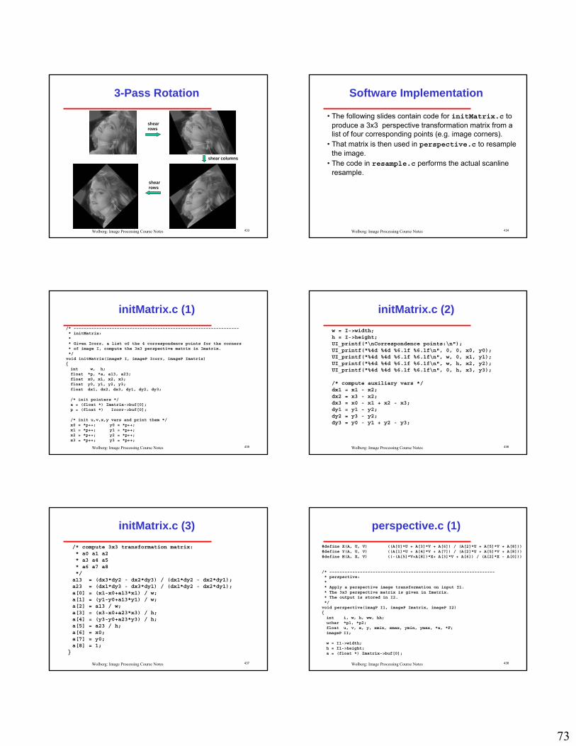
73


3-Pass Rotation

shearrows

shearrows

shear columns


Software Implementation

• The following slides contain code for initMatrix.c toproduce a 3x3 perspective transformation matrix from a list of four corresponding points (e.g. image corners).

• That matrix is then used in perspective.c to resample the image.

• The code in resample.c performs the actual scanlineresample.


initMatrix.c (1)/* ~~~~~~~~~~~~~~~~~~~~~~~~~~~~~~~~~~~~~~~~~~~~~~~~~~~~~~~~~~~~~~~~~* initMatrix:** Given Icorr, a list of the 4 correspondence points for the corners* of image I, compute the 3x3 perspective matrix in Imatrix.*/void initMatrix(imageP I, imageP Icorr, imageP Imatrix){int w, h;float *p, *a, a13, a23;float x0, x1, x2, x3;float y0, y1, y2, y3;float dx1, dx2, dx3, dy1, dy2, dy3;

/* init pointers */a = (float *) Imatrix->buf[0];p = (float *) Icorr->buf[0];

/* init u,v,x,y vars and print them */x0 = *p++; y0 = *p++;x1 = *p++; y1 = *p++;x2 = *p++; y2 = *p++;x3 = *p++; y3 = *p++;


initMatrix.c (2)w = I->width;h = I->height;UI_printf("\nCorrespondence points:\n");UI_printf("%4d %4d %6.1f %6.1f\n", 0, 0, x0, y0);UI_printf("%4d %4d %6.1f %6.1f\n", w, 0, x1, y1);UI_printf("%4d %4d %6.1f %6.1f\n", w, h, x2, y2);UI_printf("%4d %4d %6.1f %6.1f\n", 0, h, x3, y3);

/* compute auxiliary vars */dx1 = x1 - x2;dx2 = x3 - x2;dx3 = x0 - x1 + x2 - x3;dy1 = y1 - y2;dy2 = y3 - y2;dy3 = y0 - y1 + y2 - y3;


initMatrix.c (3)/* compute 3x3 transformation matrix:* a0 a1 a2* a3 a4 a5* a6 a7 a8*/a13 = (dx3*dy2 - dx2*dy3) / (dx1*dy2 - dx2*dy1);a23 = (dx1*dy3 - dx3*dy1) / (dx1*dy2 - dx2*dy1);a[0] = (x1-x0+a13*x1) / w;a[1] = (y1-y0+a13*y1) / w;a[2] = a13 / w;a[3] = (x3-x0+a23*x3) / h;a[4] = (y3-y0+a23*y3) / h;a[5] = a23 / h;a[6] = x0;a[7] = y0;a[8] = 1;

}


perspective.c (1)#define X(A, U, V) ((A[0]*U + A[3]*V + A[6]) / (A[2]*U + A[5]*V + A[8]))#define Y(A, U, V) ((A[1]*U + A[4]*V + A[7]) / (A[2]*U + A[5]*V + A[8]))#define H(A, X, V) ((-(A[5]*V+A[8])*X+ A[3]*V + A[6]) / (A[2]*X - A[0]))

/* ~~~~~~~~~~~~~~~~~~~~~~~~~~~~~~~~~~~~~~~~~~~~~~~~~~~~~~~~~~~~~~~~~* perspective:** Apply a perspective image transformation on input I1.* The 3x3 perspective matrix is given in Imatrix.* The output is stored in I2.*/

void perspective(imagP I1, imageP Imatrix, imageP I2){int i, w, h, ww, hh;uchar *p1, *p2;float u, v, x, y, xmin, xmax, ymin, ymax, *a, *F;imageP II;

w = I1->width;h = I1->height;a = (float *) Imatrix->buf[0];

74


perspective.c (2)xmin = xmax = X(a, 0, 0);x = X(a, w, 0); xmin = MIN(xmin, x); xmax = MAX(xmax, x);x = X(a, w, h); xmin = MIN(xmin, x); xmax = MAX(xmax, x);x = X(a, 0, h); xmin = MIN(xmin, x); xmax = MAX(xmax, x);

ymin = ymax = Y(a, 0, 0);y = Y(a, w, 0); ymin = MIN(ymin, y); ymax = MAX(ymax, y);y = Y(a, w, h); ymin = MIN(ymin, y); ymax = MAX(ymax, y);y = Y(a, 0, h); ymin = MIN(ymin, y); ymax = MAX(ymax, y);

ww = CEILING(xmax) - FLOOR(xmin);hh = CEILING(ymax) - FLOOR(ymin);

/* allocate mapping fct buffer */x = MAX(MAX(w, h), MAX(ww, hh));F = (float *) malloc(x * sizeof(float));if(F == NULL) IP_bailout("perspective: No memory");

/* allocate intermediate image */II = IP_allocImage(ww, h, BW_TYPE);IP_clearImage(II);p1 = (uchar *) I1->buf[0];p2 = (uchar *) II->buf[0];


perspective.c (3)/* first pass: resample rows */for(v=0; v<h; v++) {

/* init forward mapping function F; map xmin to 0 */for(u=0; u< w; u++) F[(int) u] = X(a, u, v) - xmin;

resample(p1, w, 1, F, p2);p1 += w;p2 += ww;

}

/* display intermediate image */IP_copyImage(II, NextImageP);IP_displayImage();

/* init final image */IP_copyImageHeader(I1, I2);I2->width = ww;I2->height = hh;IP_initChannels(I2, BW_TYPE);IP_clearImage(I2);


perspective.c (4)/* second pass: resample columns */for(x=0; x<ww; x++) {

p1 = (uchar *) II->buf[0] + (int) x;p2 = (uchar *) I2->buf[0] + (int) x;

/* skip past padding */for(v=0; v<h; v++,p1+=ww) {

if(*p1) break; /* check for nonzero pixel */u = H(a, (x+xmin), v); /* else, if pixel is black */if(u>=0 && u<w) break; /* then check for valid u */

}

/* init forward mapping function F; map ymin to 0 */for(i=0; v<h; v++) {

u = H(a, (x+xmin), v);u = CLIP(u, 0, w-1);F[i++] = Y(a, u, v) - ymin;

}resample(p1, i, ww, F, p2);

}IP_freeImage(II);

}


resample.c (1)/* ~~~~~~~~~~~~~~~~~~~~~~~~~~~~~~~~~~~~~~~~~~~~~~~~~~~~~~~~~~~~~~~~~~~~~~* Resample the len elements of src (with stride offst) into dst according* to the monotonic spatial mapping given in F (len entries).* The scanline is assumed to have been cleared earlier.*/

void resample(uchar *src, int len, int offst, float *F, uchar *dst){int u, uu, x, xx, ix0, ix1, I0, I1, pos;double x0, x1, dI;

if(F[0] < F[len-1])pos = 1; /* positive output stride */

else pos = 0; /* negative output stride */

for(u=0; u<len-1; u++) {/* index into src */uu = u * offst;

/* output interval (real and int) for input pixel u */if(pos) {/* positive stride */

ix0 = x0 = F[u];ix1 = x1 = F[u+1];I0 = src[uu];I1 = src[uu+offst];

}


resample.c (2)else { /* flip interval to enforce positive stride */

ix0 = x0 = F[u+1];ix1 = x1 = F[u];I0 = src[uu+offst];I1 = src[uu];

}

/* index into dst */xx = ix0 * offst;

/* check if interval is embedded in one output pixel */if(ix0 == ix1) {

dst[xx] += I0 * (x1-x0);continue;

}/* else, input straddles more than one output pixel */

/* left straddle */dst[xx] += I0 * (ix0+1-x0);


resample.c (3)

/* central interval */

xx += offst;

dI = (I1-I0) / (x1-x0);

for(x=ix0+1; x<ix1; x++,xx+=offst)

dst[xx] = I0 + dI*(x-x0);

/* right straddle */

if(x1 != ix1)

dst[xx] += (I0 + dI*(ix1-x0)) * (x1-ix1);

}

}

75

Image Warping: A Review



Objectives

• In this lecture we review digital image warping:- Geometric transformations- Forward inverse mapping- Sampling- Image reconstruction- Interpolation kernels- Separable transforms- Fant’s resampling algorithm


Definition

• Image warping deals with the geometric transformation of digital images.


Geometric Transformations

• Affine• Perspective• Bilinear• Polynomial• Splines• Elastic (local deformations)


Spatial Transformations

• Forward Mapping[x, y] = [X(u, v), Y(u, v)]

• Inverse Mapping[u, v] = [U(x, y), V(x, y)]


Forward / Inverse Mapping

u

Input image

Input image Output image

Output (accumulator) image

u xx

yv

v y

x

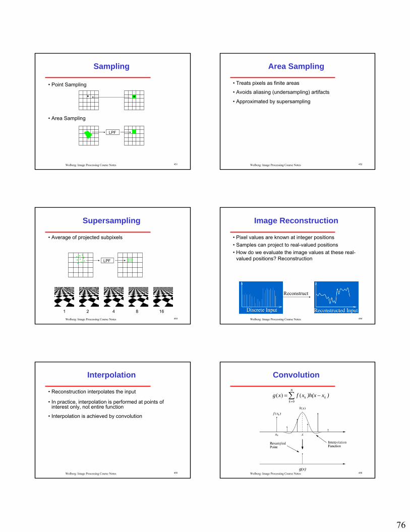
76


• Point Sampling

• Area Sampling

Sampling

LPF


Area Sampling

• Treats pixels as finite areas

• Avoids aliasing (undersampling) artifacts

• Approximated by supersampling


Supersampling

• Average of projected subpixels

LPF

1 2 4 8 16454Wolberg: Image Processing Course Notes

Image Reconstruction

• Pixel values are known at integer positions• Samples can project to real-valued positions• How do we evaluate the image values at these real-

valued positions? Reconstruction

Reconstruct


Interpolation

• Reconstruction interpolates the input

• In practice, interpolation is performed at points of interest only, not entire function

• Interpolation is achieved by convolution


Convolution

g(x)

)x)h(xxfxg k

N

kk −=∑

=0()(

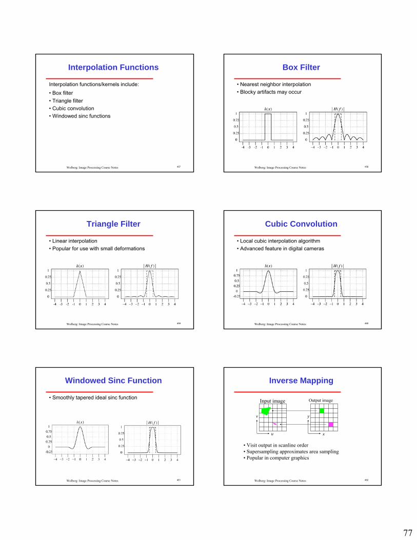
77


Interpolation Functions

Interpolation functions/kernels include:• Box filter• Triangle filter• Cubic convolution• Windowed sinc functions


Box Filter

• Nearest neighbor interpolation• Blocky artifacts may occur


Triangle Filter

• Linear interpolation• Popular for use with small deformations


Cubic Convolution

• Local cubic interpolation algorithm• Advanced feature in digital cameras


Windowed Sinc Function

• Smoothly tapered ideal sinc function


Inverse Mapping

Input image Output image

v y

x

• Visit output in scanline order• Supersampling approximates area sampling• Popular in computer graphics

u

78


Forward Mapping

Input image Output (accumulator) image

u x

yv

• Visit input in scanline order• Use output accumulator array• 2D antialiasing is difficult• Separable transforms facilitate efficient solution


Separable Transforms

• F(u, v) is a row-preserving transformation that maps all input points to their final column positions, i.e., [x, v].

• G(x, v) is a column-preserving transformation that maps the [x, v] points to their final row positions, i.e., [x, y].

),(),()],(),,([ vxGvuFvuYvuX o=


Catmull-Smith Algorithm

• First passMaps image S(u,v) into intermediate image I(x,v)

I(x,v) = S(X(u,v), v)• Second pass

Maps I(x,v) into target image T(x,y)T(x,y) = I(x, Y(Hx(v), v))

where Hx is the solution to x=X(u,v) for u


2-Pass Rotation

X, Y

G

F


2-Pass Perspective

X, Y

G

F


Fant’s Algorithm

• Forward mapping intensity resampling• Scanline order in input and output• Amenable to hardware implementation

79


Fant’s algorithm: Example (1)

XLUT

YLUT

I

YLUTx

Ix

.6 2.3 3.2 3.3 3.9

100 106

92 90100 106

115 120

100 101 105 113

101 10640 82


Fant’s algorithm: Example (2)

Ix ( ) ( )((. ))0 100 4 40= =

Ix ( ) ( ) ..

( ) ..

(( ))1 100 1 417

106 417

1 101= −⎡⎣⎢

⎤⎦⎥+ ⎡

⎣⎢⎤⎦⎥

⎡⎣⎢

⎤⎦⎥

=

Ix ( ) ( ) ..

( ) ..

((. )) ( )((. ))2 100 1 1417

106 1417

3 106 7 106= −⎡⎣⎢

⎤⎦⎥+ ⎡

⎣⎢⎤⎦⎥

⎡⎣⎢

⎤⎦⎥

+ =

Ix ( ) ( ) ..

( ) ..

((. )) ( )((. )) ( )((. ))3 106 1 79

92 79

2 92 1 90 6 82= −⎡⎣⎢

⎤⎦⎥+ ⎡

⎣⎢⎤⎦⎥

⎡⎣⎢

⎤⎦⎥

+ + =


Bibliography

• Catmull, E. and A.R. Smith, “3-D Transformations of Images in Scanline Order,” Proc. Siggraph ‘80, pp. 279-285, 1980.

• Fant, Karl M., “A Nonaliasing, Real-Time Spatial TransformTechnique,” IEEE Computer Graphics and Applications, vol. 6, no. 3, pp. 71-80, 1986.

• Wolberg, George, Digital Image Warping, IEEE Computer Society Press, Los Alamitos, CA 1990.

Image Morphing



Objectives

• In this lecture we review digital image morphing, a powerful visual effect for creating a fluid transformation from one image to another.

- Background- Morphing Algorithms

• Mesh (parametric grid)• Line pairs• Scattered points

- Examples


Inbetween Image Generation

Cross-dissolve vs. Image Morphing

sourceimagesourceimage

warpedsourceimage

warpedsourceimage

dest.imagedestdest..imageimage

warpeddest.image

warpedwarpeddestdest..imageimage

cross-dissolvecross-dissolve

image morphingimage morphing

80


Mesh Warp (1)


Mesh Warp (2)

Source / Target Meshes


Mesh Warp (3)

Intermediate Mesh


Mesh Warp (4)

Horizontal Resampling


Mesh Warp (5)

Vertical Resampling


Line Warp (1)

v X P Perp Q PQ P

= − ⋅ −−

( ) ( )

X

Q

P

u

v

Destination Image

Q’

X’

P’

v

u

Source Image

u X P Q PQ P

= − ⋅ −−

( ) ( )2

′ = ′ + ⋅ ′ − ′ + ⋅ ′ − ′′ − ′

X P u Q P v Perp Q PQ P

( ) ( )

81


Line Warp (2)

X

Q1

P1

u1

v1

Destination Image

QQ11’’

XX

PP11’’

vv11

uu11

Source Image

PP22

Q2

v2

u2

QQ22’’

PP22’’

uu22

vv22

XX’’XX11’’XX22’’


Scattered Point Constraints

Treat correspondence data as scattered data:[x,y] = [X(u,v), Y(u,v)]

uv

X(u,v)


Example


Uniform Transition


Nonuniform Transition


Morph Sequence

82


Morph Sequence


Bibliography• Beier, T. and S. Neely, “Feature-Based Image Metamorphosis,” Proc. Siggraph ‘92, pp. 35-42,

1992.

• Smythe, D., “A Two-Pass Mesh Warping Algorithm for Object Transformation and Image Interpolation,” ILM Technical Memo #1030, Computer Graphics Dept., Lucasfilm Ltd., 1990.

• Lee, S., K.Y. Chwa, S.Y. Shin, and G. Wolberg, “Image Metamorphosis Using Snakes and Free-Form Deformations,” Proc. Siggraph ‘95, pp. 439-448, 1992.

• Lee, S., G. Wolberg, K.Y. Chwa, and S.Y. Shin, “Image Metamorphosis with Scattered Feature Constraints,” IEEE Trans. Visualization and Computer Graphics, vol. 2, no. 4, pp. 337-354, 1996.

• Wolberg, G., “Image Morphing: A Survey”, Visual Computer, vol. 14, no. 8/9, pp. 360-372, 1998.

• Wolberg, G., Digital Image Warping, IEEE Computer Society Press, Los Alamitos, CA 1990.

Robust Log-Polar Registration



Objectives

• In this lecture we review image registration, a process to align multiple images together.

- Affine registration- Perspective registration- Polar coordinates- Log-polar algorithm- Examples


Introduction

• Image registration refers to the problem of aligning a set of images.

• The images may be taken at different times, by different sensors, or from different viewpoints.


Applications

• Multisensor data fusion- integrating information taken from different sensors

• Image analysis / surveillance / change detection- for images taken at different times/conditions

• Image mosaics- generating large panoramas from overlapping images

• Super-resolution images / noise removal- integrating multiple registered images

83


Geometric Transformations

Geometric transformation models for registration:• Rigid transformation

- translation, rotation (3 parameters)

• Affine transformation- translation, rotation, scale, shear (6 parameters)

• Perspective transformation- affine, perspective foreshortening (8 parameters)

• Local transformation- terrain relief, nonlinear, nonrigid


Parameter Estimation (1)

Moderate perspective|β|, |γ| < 40o

Severe perspective40o < |β|, |γ| < 90o


Parameter Estimation (2)

The objective function (similarity measure):

Q{} is the affine or perspective transform applied to image I2. We use the Levenberg-Marquardt method to minimize the above objective function for each pyramid level.

∑=

−=N

i

yxQIyxI1

2''a21

2 })),{(),(()(aχ


Affine Registration

Image I1 Image I2 I2 registered to I1

Actual parameters: RST = (30°, 1.5, 30, 30)Estimated parameters: RST = (29.99°, 1.51, 29.51, 30.66)


Local Affine Approximation

2 X 2 tiles 4 X 4 tiles


Piecewise Affine Approximation

• Consider I2 subdivided into a regular grid of tiles• For each tile Ti

2 search for similar tile Ti1 in I1 by

performing affine registration using LMA• Get collection of affine parameters and tile centers• Plug into system of equations• Solve for 8 persp. parameters using the pseudoinverse

84


Example (1)


Example (1)


Perspective Registration


• The camera's flash introduces a highlight.• Each highlight will appear at a different location on each

image when captured from different viewpoints.• If we register these images onto a common frame, we can

render the final image by fusing the registered images.

Glare Removal


•Video mosaic

Example (2)


•Video stabilization

Example (3)

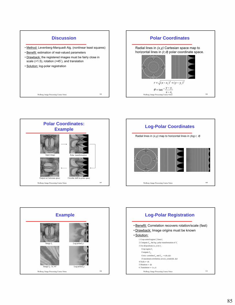
85


Discussion

• Method: Levenberg-Marquadt Alg. (nonlinear least squares)• Benefit: estimation of real-valued parameters• Drawback: the registered images must be fairly close in

scale (<1.5), rotation (<45°), and translation• Solution: log-polar registration


Polar Coordinates

Radial lines in (x,y) Cartesian space map to horizontal lines in (r,θ) polar coordinate space.

c

c

cc

xxyy

yyxxr

−−=

−+−=

−1

22

tan

)()(

θ


Polar Coordinates: Example

Input image Polar transformation

Circular shift in polar spaceOutput in Cartesian space


Log-Polar Coordinates

Radial lines in (x,y) map to horizontal lines in (log r, θ)


Example

Image I1 Log-polar(I1)

Log-polar(I2)Image I2: 3x; 45°


Log-Polar Registration

• Benefit: Correlation recovers rotation/scale (fast)• Drawback: Image origins must be known• Solution:

),(nTranslatio .6Rotation .5Scale .4

and save n,correlatio maximum if

),( and correlate-Cross

Compute

region Crop

:in ),( positions allFor 3.

of sformationpolar tran-log the, Compute .2

from region central Crop 1.

'2

'1

'2

'2

2

'1

'1

1'1

yxdy

dx(dx, dy)(x, y)

dydxII

I

I

Iyx

II

II

pp

p

p

←←

←

→

86


Scanning Window


Example


Example

Rotation = -21°Scale = 0.469Translation = (-11,-51)


Biological Motivations (1)

• Despite the difficulties of nonlinear processing, the log-polar transform has received considerable attention. [Marshal41] et. al. and [Hubel74] discovered a log-polar mapping in the primate visual system and this conformal map is an accepted model of the representation of the retina in the primary visual cortex in primates [Schwartz79] [Weinshall87].



The left figure shows contours of cone cell density. In fact, the density of the ganglion cells which transmit information out of the retina is distributed logarithmically. From Osterberg, G. (1935)

Benefits:1. Reduce the amount of information traversing the optical nerve while maintaining high resolution in the fovea and capturing a wide field of view in the periphery.

2. Invariant to scale and rotation.516Wolberg: Image Processing Course Notes


Fovea based vision

87


Related Work• The Fourier-Mellin transform uses log-polar mapping to align

images related by scale, rotation, and translation {Casasent76, Decastro87, Chen94, Reddy96,

Lucchese96, Chang97, Lucchese97a, Lucchese97b, Stone99, Stone03, Keller03}.

• Detect lines in log-Hough space {Weiman79, Giesler98, Weiman90, Young00}.

• Recognizing 2D objects that were arbitrarily rotated or scaled {Sandini92, Ferrari95}.

• Tracking a moving object {Capurro97}.• Estimation of time-to-impact from optical flow {Sandini91}• Finding disparity map in stereo images {Sandini01}.• Using log-polar transform to calculate time-to-crash for mobile

vehicles {Pardo02}.• A foveated binocular stereo system using log polar transforms

{Bernardino02}.


Previous work: Fourier-Mellin

• The magnitude of spectra |F1| is a rotated and scaled replica of |F2|. We can recover this rotation and scale by representing the spectra |F1| and |F2| in log-polar coordinates:

• Phase-correlation can be used to recover the amount shift

)(000021

00000021

00))cos()sin(

,)sin()cos(

(1),(

)))cos()sin((),)sin()cos(((),(

yx yxJyxyxyx e

ssF

sF

yyxsxyxsIyxI

ωωθωθωθωθωωω

θθθθ

++−+=

−+−−+=

),log(log1),(log 021 θθθ −+= srFs

rF


Previous work: Fourier-Mellin• Example: s = 1.5, θ = 36◦



•Benefit: We can search for the scale and rotation independent of the translations.

•Drawbacks: Large translation, scale, or mild perspective will alter the coefficients of the finite and discrete Fourier transform.



(a) Reference image (b) Target image (real) (c) Target image (synthetic)

Power spectra of (a), (b), and (c) 522Wolberg: Image Processing Course Notes

Example from INRIA

88


Example (1)


Example (2)


Example (3)

Reference image Target imageRecovered parameters:θ = 228.17◦ , S = 3.528217

Tx=-32 Ty=35


Example: Large Perspective (1)


Example: Large Perspective (2)


Summary

•Log-polar registration:- recovers large-scale rotation/scale/translation- applies fast correlation in log-polar space- exploits fast multiresolution processing- initial estimate for affine/perspective registration

•Perspective registration:- handles small distortions with subpixel accuracy- applies Levenberg-Marquardt algorithm- nonlinear least squares optimization- exploits fast multiresolution processing

IMAGE PROCESSING - Computer Sciencewolberg/cs4165/doc/CSc470.pdf · 1 Introduction to Image...

Documents

Transcript of IMAGE PROCESSING - Computer Sciencewolberg/cs4165/doc/CSc470.pdf · 1 Introduction to Image...