Image Display and HistogramsFor students of HI 5323 “Image Processing”

Willy Wriggers, Ph.D.School of Health Information Sciences

http://biomachina.org/courses/processing/02.html

T H E U N I V E R S I T Y of T E X A S

H E A L T H S C I E N C E C E N T E R A T H O U S T O N

S C H O O L of H E A L T H I N F O R M A T I O N S C I E N C E S

Properties of Displays

• Size and # of Pixels

• Brightness

• Linearity

• Flatness

• Resolution

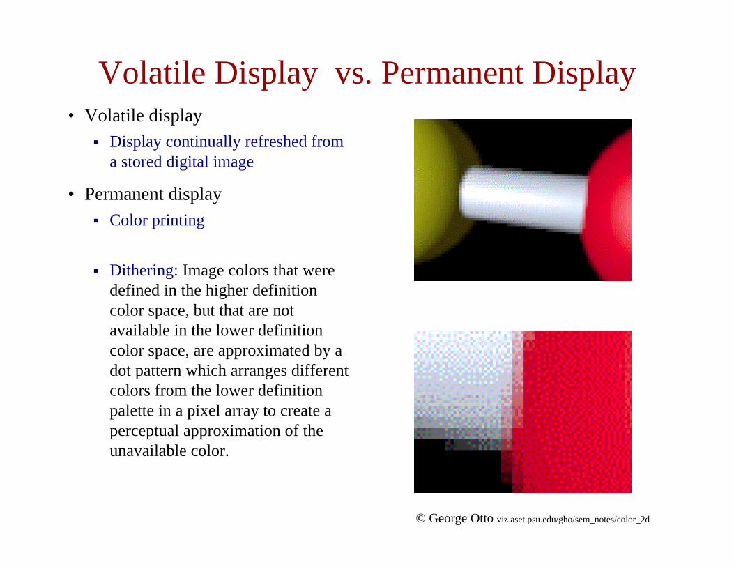
Volatile Display vs. Permanent Display• Volatile display

Display continually refreshed from a stored digital image

• Permanent displayColor printing

Dithering: Image colors that were defined in the higher definition color space, but that are not available in the lower definition color space, are approximated by a dot pattern which arranges different colors from the lower definition palette in a pixel array to create a perceptual approximation of the unavailable color.

© George Otto viz.aset.psu.edu/gho/sem_notes/color_2d

Intensity Discrimination

• Human eye can discriminate 1000 shades of gray

• For constant adaptation, about 200 levels

• 8 bits 2 = 256 shades8

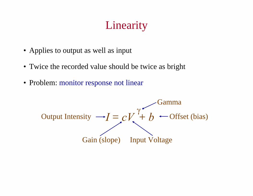
γI = cV + b

Linearity

• Applies to output as well as input

• Twice the recorded value should be twice as bright

• Problem: monitor response not linear

Output Intensity Offset (bias)

Gain (slope) Input Voltage

Gamma

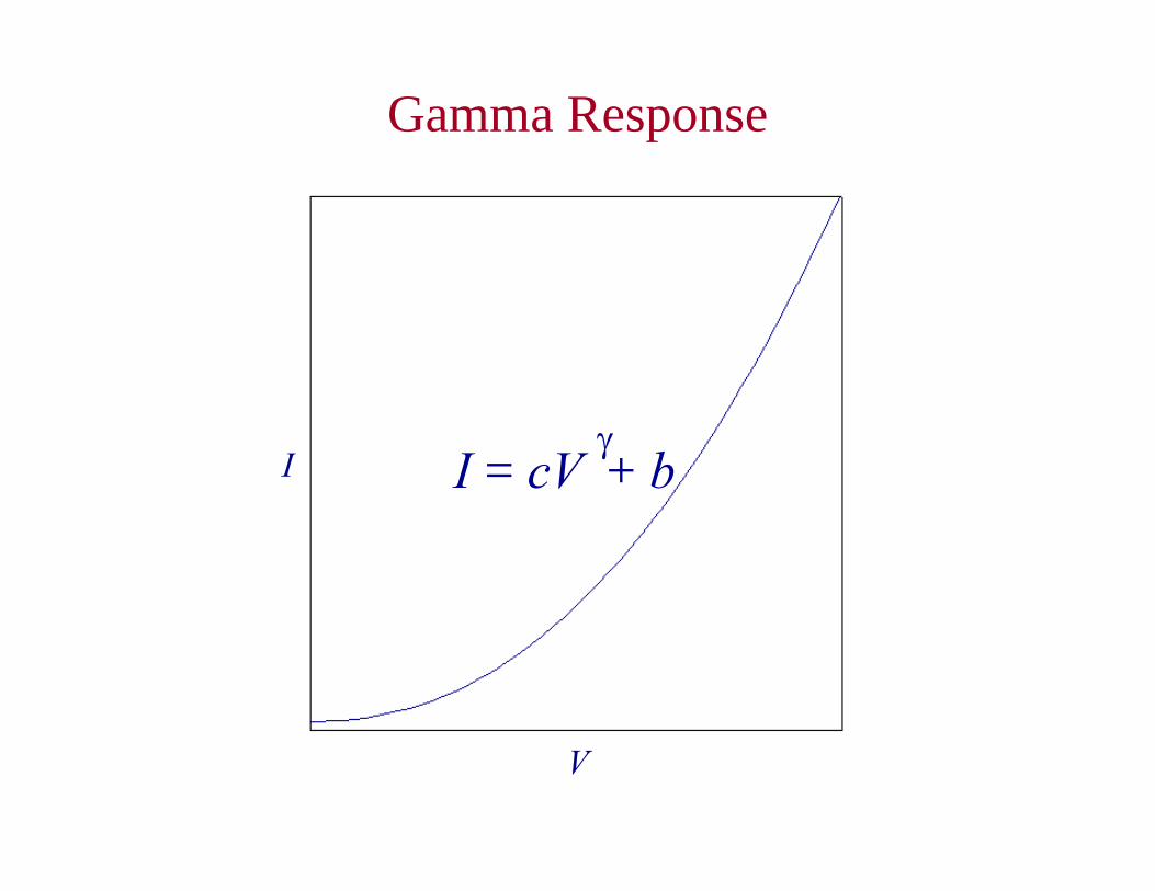
Gamma Response

V

Iγ

I = cV + b

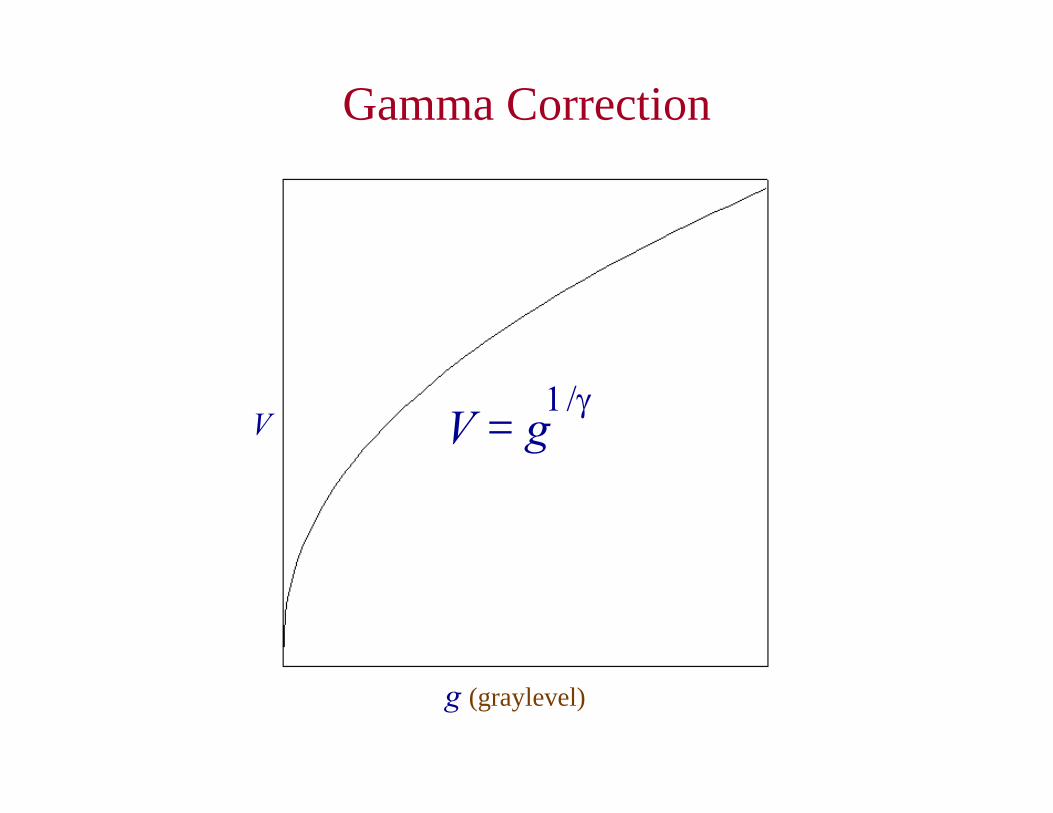
Gamma Correction

g (graylevel)

V1/γ

V = g

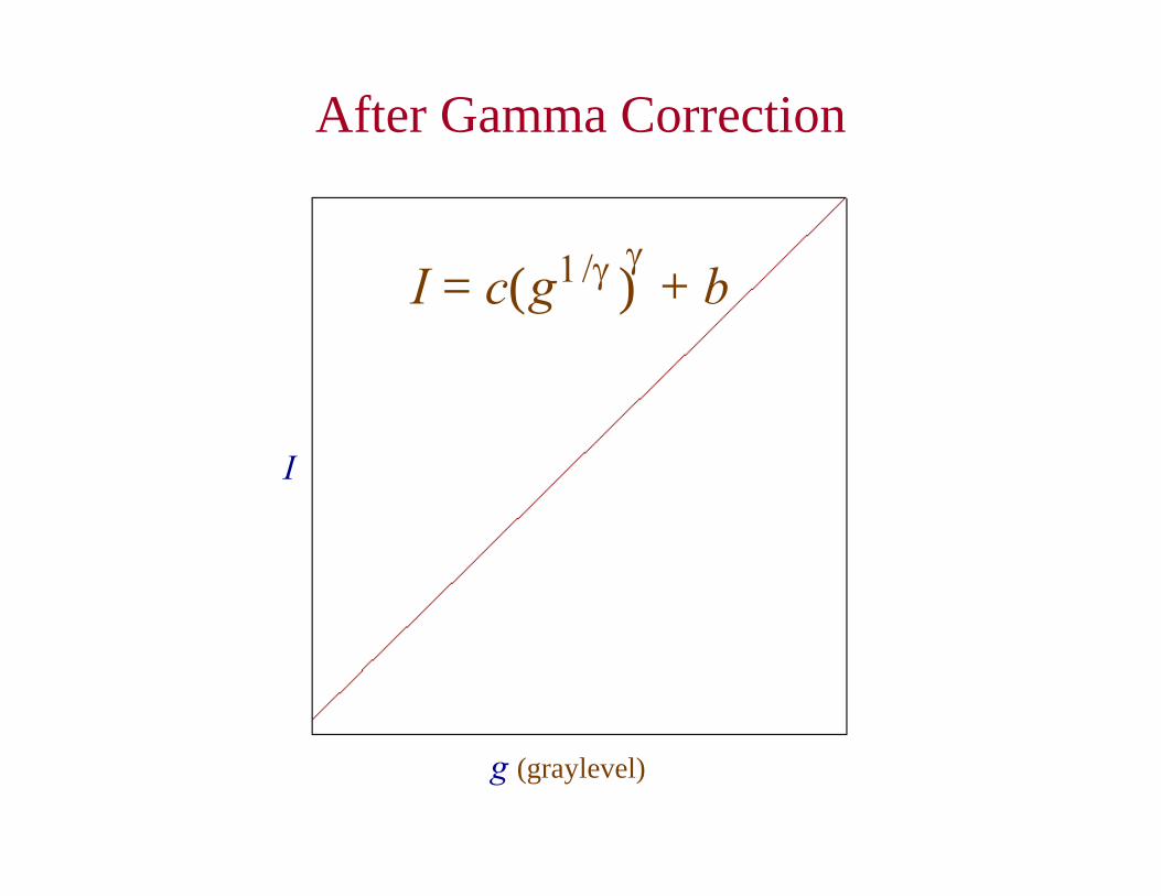
After Gamma Correction

g (graylevel)

I

γI = c( ) + b1/γg

Gamma Correction

• Different monitors have different gammas

• Be careful of different operating systems, drivers, etc.

• Applies to imaging devices as well: cameras, scanners, etc.

Gaussian Spots

222 )(),( ryx eeyxp −+− ==

• R radius at which intensity drops to ½ maximum

22)/(

22

)/()2ln(

)2ln()/(

2

)(

Rr

Rrr

Rre

eerp

−

−−

==

==−

• Digital display devices generate output via a collection of dots/spots

• Each spot has a 2-D intensity distribution:Modeled as a radially symmetric Gaussian

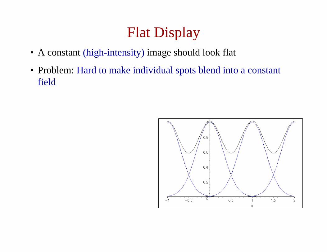
Flat Display• A constant (high-intensity) image should look flat

• Problem: Hard to make individual spots blend into a constant field

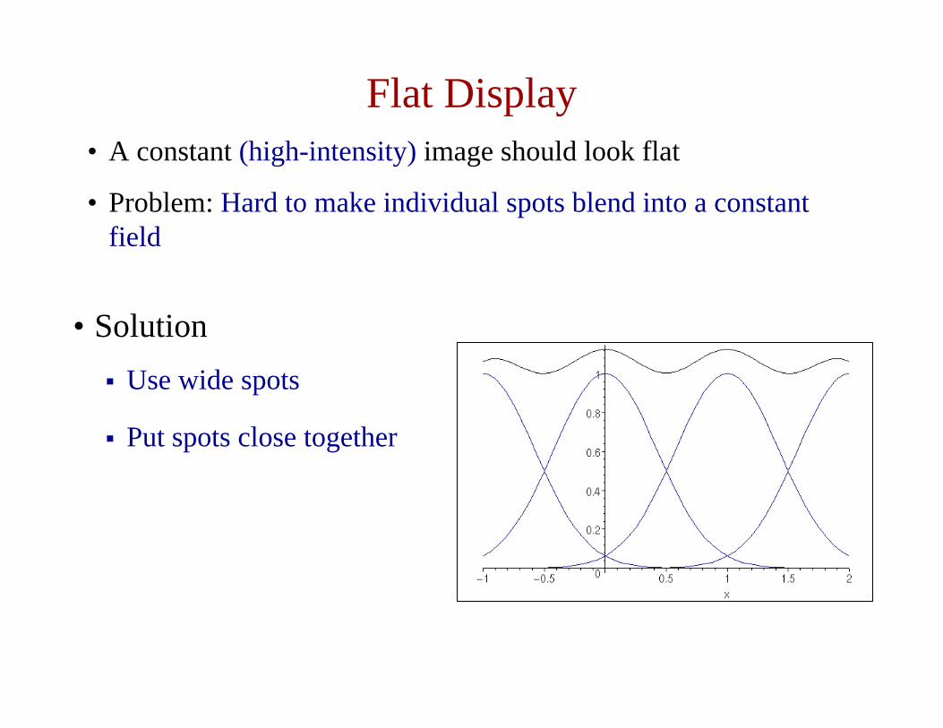
Flat Display• A constant (high-intensity) image should look flat

• Problem: Hard to make individual spots blend into a constant field

• Solution

Put spots close together

Use wide spots

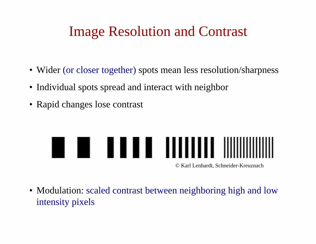
Image Resolution and Contrast

• Wider (or closer together) spots mean less resolution/sharpness

• Individual spots spread and interact with neighbor

• Rapid changes lose contrast

• Modulation: scaled contrast between neighboring high and low intensity pixels

© Karl Lenhardt, Schneider-Kreuznach

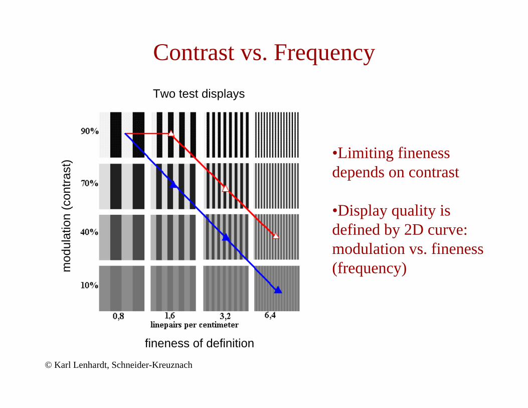
Contrast vs. Frequency

© Karl Lenhardt, Schneider-Kreuznach

Two test displays

mod

ulat

ion

(con

trast

)

fineness of definition

•Limiting fineness depends on contrast

•Display quality is defined by 2D curve: modulation vs. fineness (frequency)

Modulation Contrast Function

• Instead of line pairs, use sine waves

• Measure contrast (modulation) as a function of spatial frequencyof sine wave

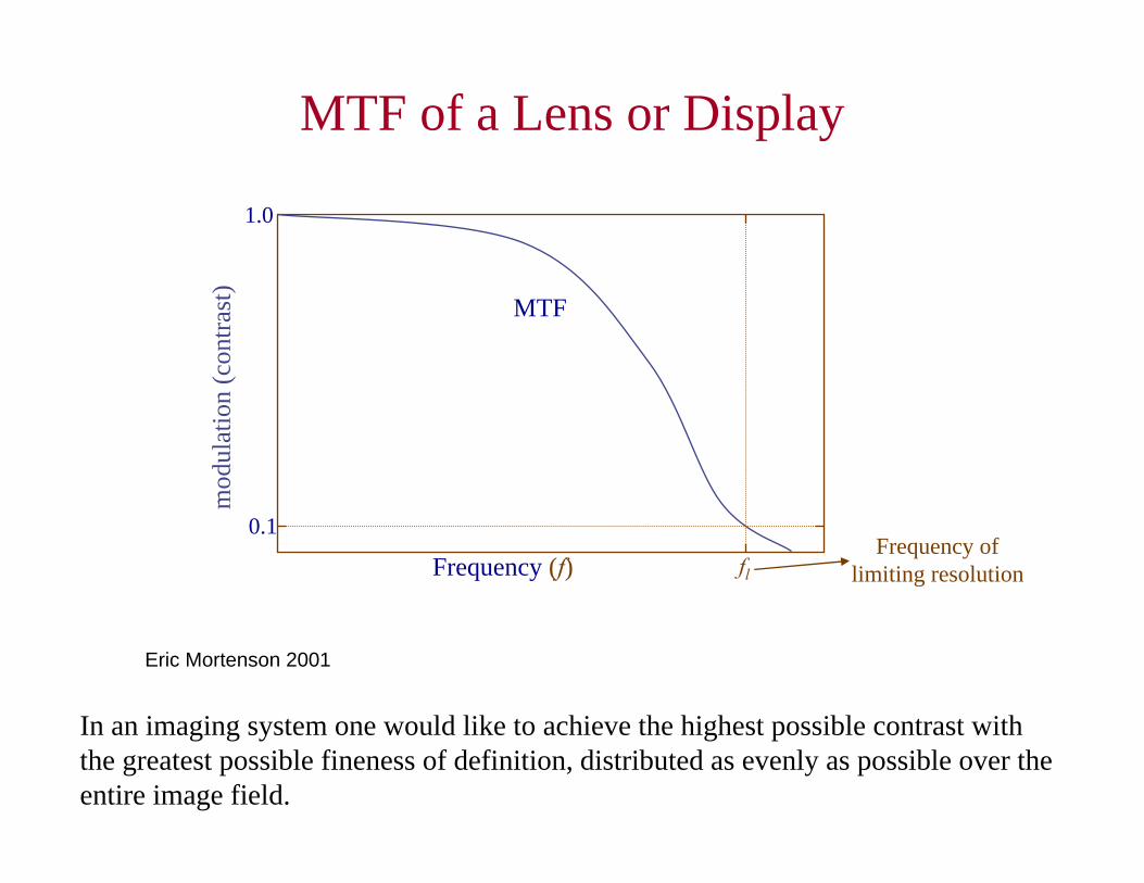
MTF of a Lens or Display

Frequency (f)

MTF

fl

1.0

Frequency oflimiting resolution

0.1

Eric Mortenson 2001

mod

ulat

ion

(con

trast

)

In an imaging system one would like to achieve the highest possible contrast with the greatest possible fineness of definition, distributed as evenly as possible over the entire image field.

Noise

• Intensity of display spotRandom noisePeriodic and synchronized noise

• Position of display spotEffects of spot interaction + position noise

Reconstruction

• Reverse of digitization:

• Undo sampling: or at least make is seem continuousGaussian spotsResampling

• Undo quantization: convert back to analogInterpolationDithering

Interpolation

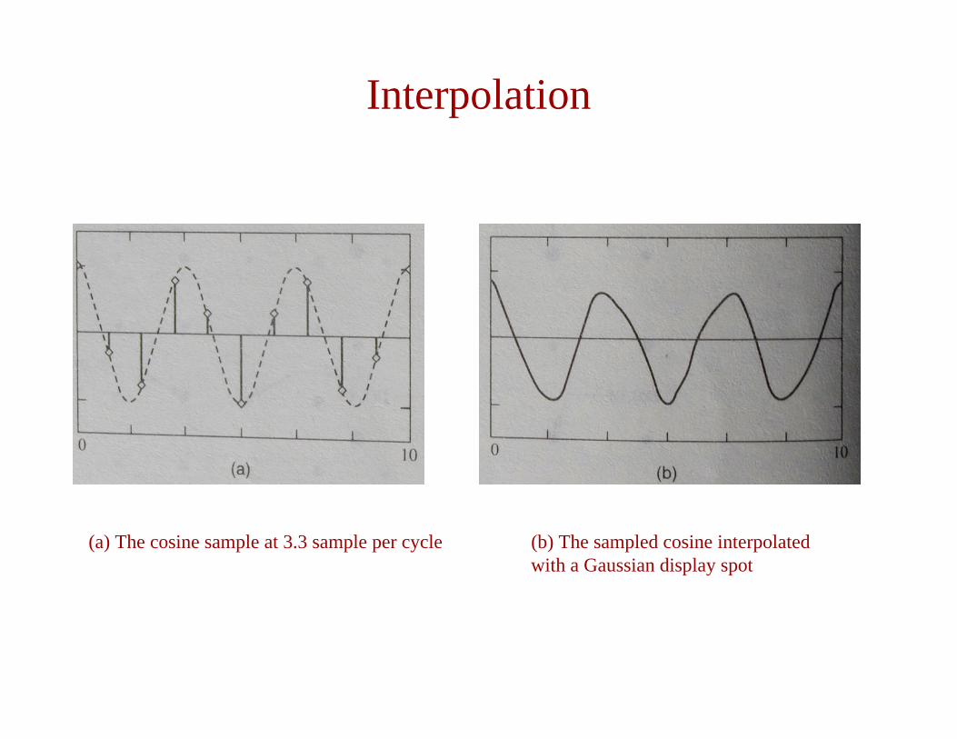
(a) The cosine sample at 3.3 sample per cycle (b) The sampled cosine interpolated with a Gaussian display spot

Oversampling & Resampling

• The inappropriate shape of the Gaussian display spot has less effect when there are more sample points per cycle of the cosine

Oversamplingtradeoff – more expensive

Resampling- The process of increasing the size of the image by digitally implemented

interpolation prior to displaying it- A 512 x 512 image might be interpolated up to 1024 x 1024, then displayed on

a monitor with a Gaussian display spot

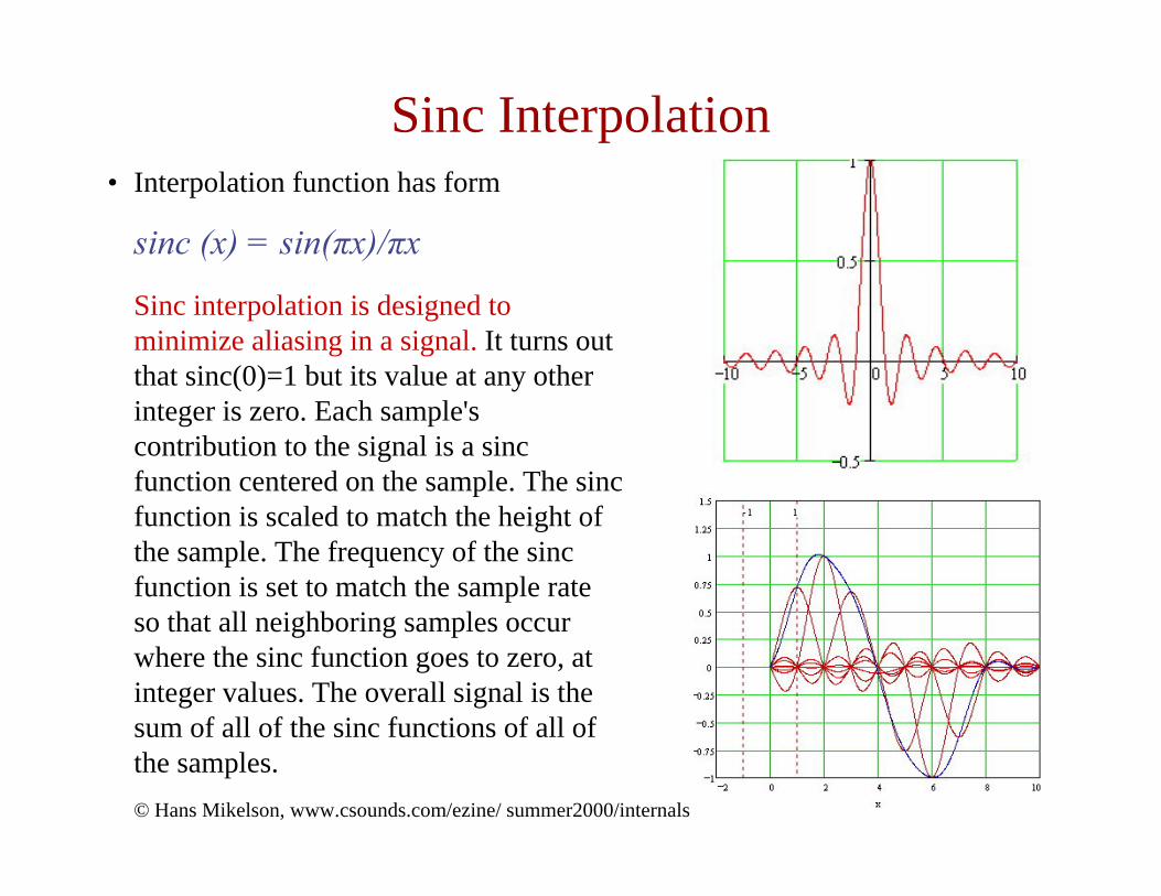
Sinc Interpolation • Interpolation function has form

sinc (x) = sin(πx)/πx

Sinc interpolation is designed to minimize aliasing in a signal. It turns out that sinc(0)=1 but its value at any other integer is zero. Each sample's contribution to the signal is a sincfunction centered on the sample. The sincfunction is scaled to match the height of the sample. The frequency of the sincfunction is set to match the sample rate so that all neighboring samples occur where the sinc function goes to zero, at integer values. The overall signal is the sum of all of the sinc functions of all of the samples. © Hans Mikelson, www.csounds.com/ezine/ summer2000/internals

Histograms• Histograms count the number of occurrences of each graylevel

value

H(D)

Count Graylevel

H(D)

Trees &Barn Walls Grass

BarnRoof

Sky

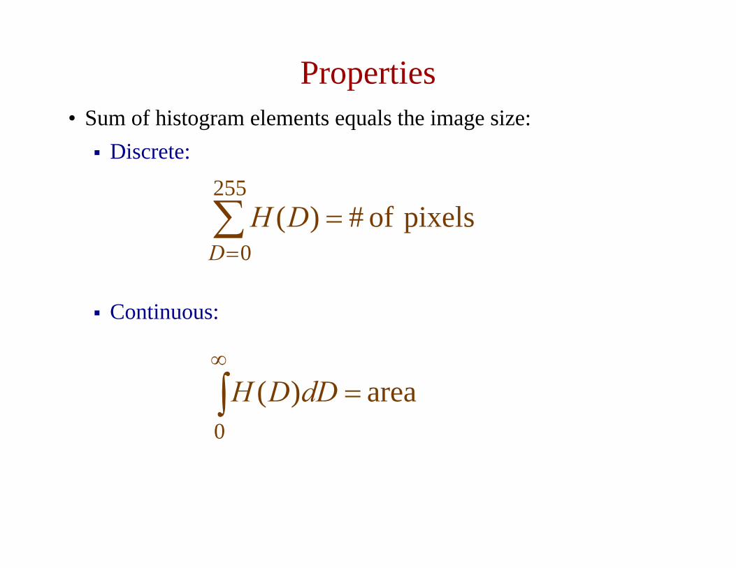
Properties• Sum of histogram elements equals the image size:

Discrete:

Continuous:

pixels of # )(255

0∑=

=D

DH

area )(0∫∞

=dDDH

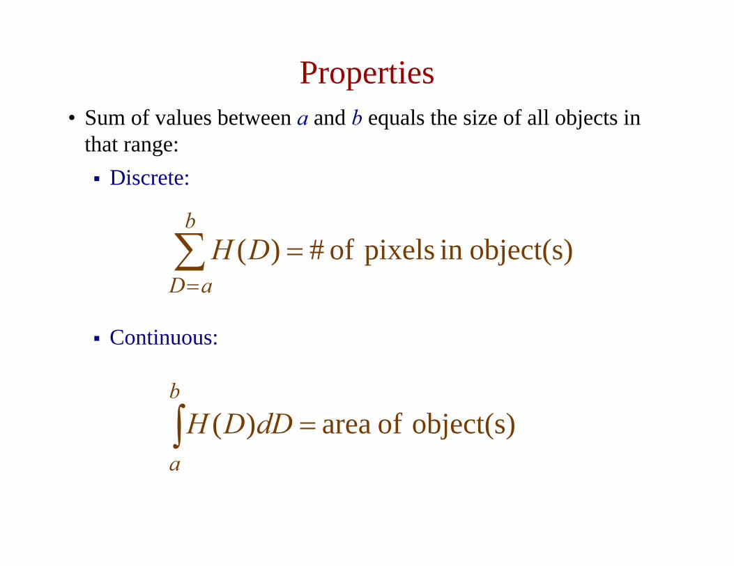
Properties• Sum of values between a and b equals the size of all objects in

that range:Discrete:

Continuous:

object(s)in pixels of # )(∑=

=b

aDDH

object(s) of area )(∫ =b

a

dDDH

Properties• Integrated optical density: weight of image (or objects)

• Mean graylevel: average intensity in image (or objects)

∫=b

a

dDDDHIOD )(

∫

∫== b

a

b

a

dDDH

dDDDH

areaIODMGL

)(

)(

Application: Camera Parameters

• Too Bright: lots of pixels at 255 (or max)

• Too Dark: lots of pixels at 0

• Gain Too Low: not enough of the range used

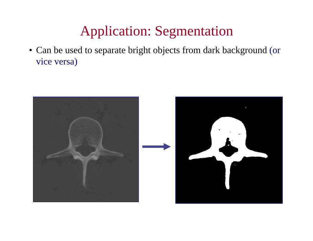
Application: Segmentation• Can be used to separate bright objects from dark background (or

vice versa)

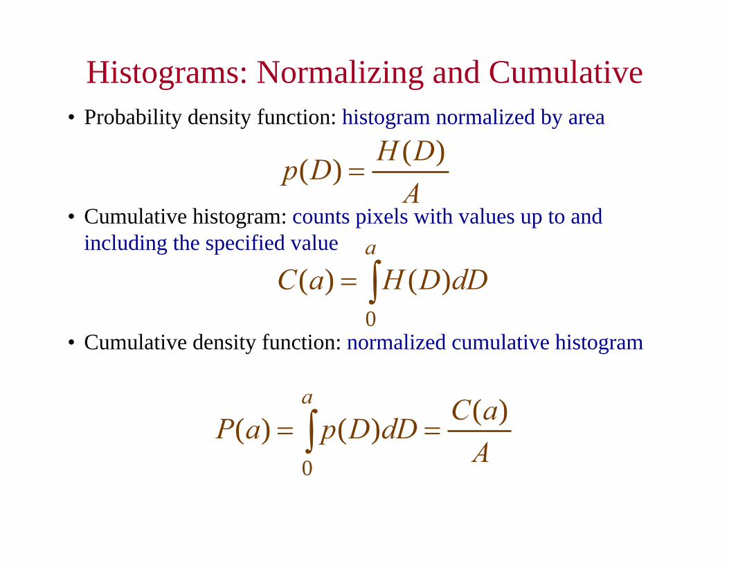
Histograms: Normalizing and Cumulative• Probability density function: histogram normalized by area

• Cumulative histogram: counts pixels with values up to and including the specified value

• Cumulative density function: normalized cumulative histogram

ADHDp )()( =

∫=a

dDDHaC0

)()(

AaCdDDpaP

a )()()(0

== ∫

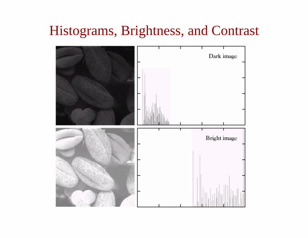
Histograms, Brightness, and Contrast

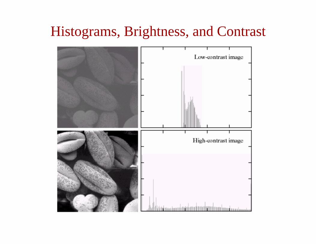
Histograms, Brightness, and Contrast

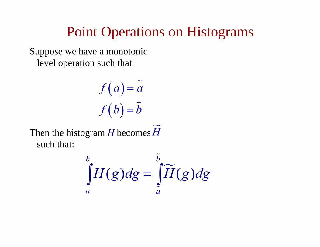
Point Operations on HistogramsSuppose we have a monotonic

level operation such that

Then the histogram H becomes such that:

( )( )

f a a

f b b

=

=

( ) ( )b b

a a

H g dg H g dg=∫ ∫

H

Point Operations on Histograms

Let b = a + ∆ for some very small ∆,

then

Thus

or approximating the last expression to first order:

( )

( ) ( )a f aa

a a

H g dg H g dg′+ ∆+∆

=∫ ∫

1

1

( ) ( ) ( ) ; ( ) ( )( ) ; ( )( ) ( )( ( ))( )( ( ))

H a H a f aH a H aH a g a f af a f aH f gH gf f g

−

−

′∆ ≈ ∆ ⇒∆

≈ = ≡ = ⇒′ ′∆

=′

∆′+≈ )()()( afafbf

Histogram Equalization

Automatic contrast enhancement:Basic Idea: allocate the most output levels to the most frequently occurring inputsLook at the histogram of the input signalIf we allocate output levels proportional to the frequency of occurrence for our input levels, the output histogram should be uniformThis process is know as histogram equalization

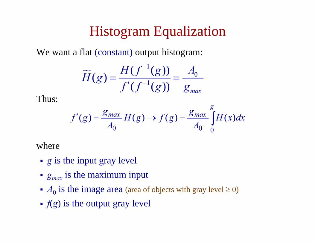
Histogram EqualizationWe want a flat (constant) output histogram:

Thus:

whereg is the input gray levelgmax is the maximum inputA0 is the image area (area of objects with gray level ≥ 0)

f(g) is the output gray level

10

1

( ( ))( )( ( )) max

AH f gH gf f g g

−

−= =′

∫=→=′g

maxmax dxxHA

ggfgHA

ggf000

)()()()(

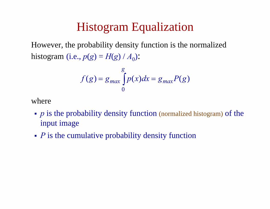
Histogram EqualizationHowever, the probability density function is the normalized histogram (i.e., p(g) = H(g) / A0):

wherep is the probability density function (normalized histogram) of the input imageP is the cumulative probability density function

)()()(0

gPgdxxpggf max

g

max == ∫

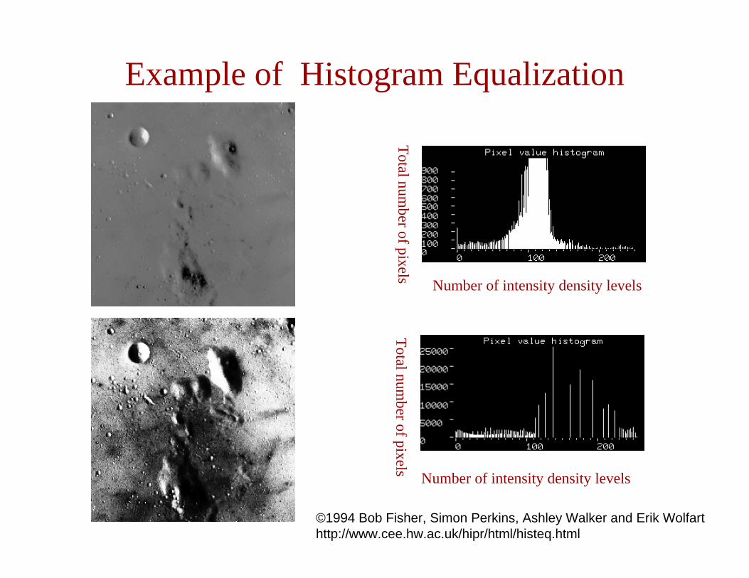
Example of Histogram Equalization

Total number of pixels

Number of intensity density levels

Total number of pixels

Number of intensity density levels

©1994 Bob Fisher, Simon Perkins, Ashley Walker and Erik Wolfarthttp://www.cee.hw.ac.uk/hipr/html/histeq.html

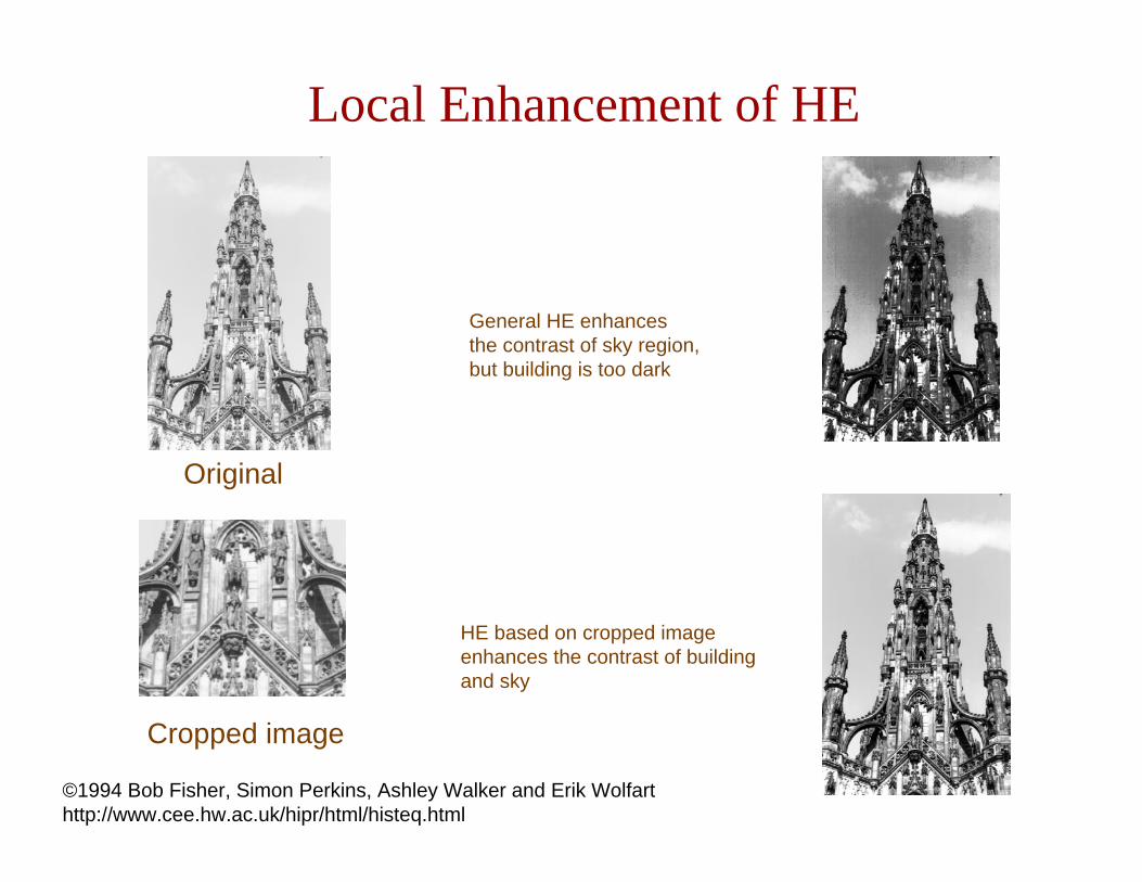
Local Enhancement of HE

Original

Cropped image

General HE enhances the contrast of sky region,but building is too dark

HE based on cropped image enhances the contrast of building and sky

©1994 Bob Fisher, Simon Perkins, Ashley Walker and Erik Wolfarthttp://www.cee.hw.ac.uk/hipr/html/histeq.html

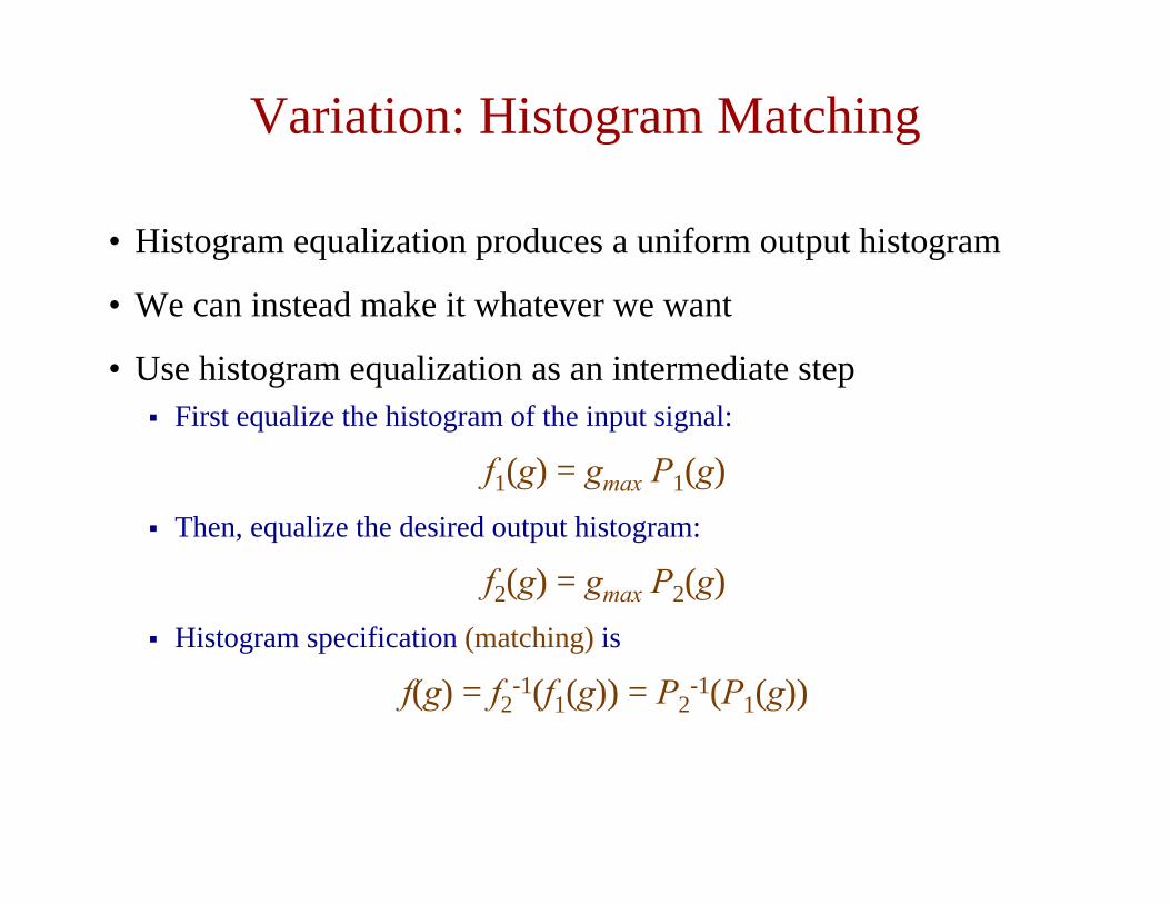
Variation: Histogram Matching

• Histogram equalization produces a uniform output histogram

• We can instead make it whatever we want

• Use histogram equalization as an intermediate stepFirst equalize the histogram of the input signal:

f1(g) = gmax P1(g)Then, equalize the desired output histogram:

f2(g) = gmax P2(g)Histogram specification (matching) is

f(g) = f2-1(f1(g)) = P2

-1(P1(g))

Figure and Text Credits Text and figures for this lecture were adapted in part from the following source, in agreement with the listed copyright statements:

http://web.engr.oregonstate.edu/~enm/cs519© 2003 School of Electrical Engineering and Computer Science, Oregon State University, Dearborn Hall, Corvallis, Oregon, 97331

Resources

Textbooks:Kenneth R. Castleman, Digital Image Processing, Chapter 3, 5John C. Russ, The Image Processing Handbook, Chapter 3, 4

Resources and Reading Assignment

Textbooks:Kenneth R. Castleman, Digital Image Processing, Chapter 6, 7, 8John C. Russ, The Image Processing Handbook, Chapter 5