IEEE TRANSACTIONS ON CONTROL SYSTEMS TECHNOLOGY…acl.mit.edu/papers/KuwataTCST09.pdf · ·...

IEEE TRANSACTIONS ON CONTROL SYSTEMS TECHNOLOGY, VOL. 17, NO. 5, SEPTEMBER 2009 1105

Real-time Motion Planning with Applications toAutonomous Urban Driving

Yoshiaki Kuwata, Member, IEEE, Justin Teo, Student Member, IEEE,Gaston Fiore, Student Member, IEEE, Sertac Karaman, Student Member, IEEE,

Emilio Frazzoli, Senior Member, IEEE, and Jonathan P. How, Senior Member, IEEE

Abstract—This paper describes a real-time motion planningalgorithm, based on the Rapidly-exploring Random Tree (RRT)approach, applicable to autonomous vehicles operating in anurban environment. Extensions to the standard RRT are predom-inantly motivated by: (i) the need to generate dynamically feasibleplans in real-time, (ii) safety requirements, (iii) the constraintsdictated by the uncertain operating (urban) environment. Theprimary novelty is in the use of closed-loop prediction in theframework of RRT. The proposed algorithm was at the core of theplanning and control software for Team MIT’s entry for the 2007DARPA Urban Challenge, where the vehicle demonstrated theability to complete a 60 mile simulated military supply mission,while safely interacting with other autonomous and human drivenvehicles.

Index Terms—Real-time motion planning, dynamic and un-certain environment, RRT, urban driving, autonomous, DARPAUrban Challenge.

I. INTRODUCTION

In November 2007, several autonomous automobiles fromall over the world competed in the DARPA Urban Challenge(DUC), which was the third installment of a series of racesfor autonomous ground robots [1]. Unlike previous events thattook place on desert dirt roads, the DUC course consistedmainly of paved roads, incorporating features like intersec-tions, rotaries, parking lots, winding roads, and highways,typically found in urban/suburban environments. The majordistinguishing characteristic of the DUC was the introductionof traffic, with up to 70 robotic and human-driven vehicleson the course simultaneously. This resulted in hundreds ofunscripted robot-on-robot (and robot on human-driven vehi-cle) interactions. With a longer term goal of fielding suchautonomous vehicles in environments with co-existing trafficand/or traffic infrastructure, all vehicles were required to abideby the traffic laws and rules of the road. Vehicles were

Y. Kuwata was with Department of Aeronautics & Astronautics, Mas-sachusetts Institute of Technology, Cambridge, MA, 02139 USA. He is nowwith Jet Propulsion Laboratory, California Institute of Technology, Pasadena,CA, 91109 USA. e-mail: [email protected].

J. Teo, E. Frazzoli and J. How are with Department of Aeronautics &Astronautics, Massachusetts Institute of Technology, Cambridge, MA, 02139USA. e-mail: {csteo, frazzoli, jhow}@mit.edu.

G. Fiore was with Department of Aeronautics & Astronautics, Mas-sachusetts Institute of Technology, Cambridge, MA, 02139 USA. He isnow with School of Engineering and Applied Sciences, Harvard University,Cambridge, MA, 02138 USA. e-mail: [email protected].

S. Karaman is with Department of Mechanical Engineering, Mas-sachusetts Institute of Technology, Cambridge, MA, 02139 USA. e-mail:[email protected].

Manuscript received September 12, 2008; revised December 23, 2008.

expected to stay in the correct lane, maintain a safe speed at orunder specified speed limits, correctly yield to other vehicles atintersections, pass other vehicles when safe to do so, recognizeblockages and execute U-turns when needed, and park in anassigned space.

Developing a robotic vehicle that could complete the DUCwas a major systems engineering effort, requiring the de-velopment and integration of state-of-the-art technologies inplanning, control, and sensing [2], [3]. The reader is referredto [3] for a system-level report on the design and developmentof Team MIT’s vehicle, Talos. The focus of this paper is onthe motion planning subsystem (or “motion planner”) and theassociated controller (which is tightly coupled with the motionplanner). The motion planner is an intermediate level planner,with inputs primarily from a high level planner called theNavigator, and outputs being executed by the low level con-troller. Given the latest environment information and vehiclestates, the motion planner computes a feasible trajectory toreach a goal point specified by the Navigator. This trajectoryis feasible in the sense that it avoids static obstacles and othervehicles, and abide by the rules of the road. The output of themotion planner is then sent to the controller, which interfacesdirectly to the vehicle, and is responsible for the execution ofthe motion plan.

The main challenges in designing the motion planningsubsystem resulted from the following factors: (i) complex andunstable vehicle dynamics, with substantial drift, (ii) limitedsensing capabilities, such as range and visibility, in an uncer-tain, time-varying environment, and (iii) temporal and logicalconstraints on the vehicle’s behavior, arising from the rules ofthe road.

Numerous approaches to address the motion planning prob-lem have been proposed in the literature, and the readeris referred to [1], [4]–[8], to name a few. For our motionplanning system, we chose to build it on the Rapidly-exploringRandom Trees (RRT) algorithm [9]–[11], which belongs to theclass of incremental sampling-based methods [7, Section 14.4].The main reasons for this choice were: (i) sampling-basedalgorithms are applicable to very general dynamical models,(ii) the incremental nature of the algorithms lends itself easilyto real-time, on-line implementation, while retaining certaincompleteness guarantees, and (iii) sampling-based methods donot require the explicit enumeration of constraints, but allowtrajectory-wise checking of possibly very complex constraints.

In spite of their generality, the application of incrementalsampling-based motion planning methods to robotic vehicles


with complex and unstable dynamics, such as the full-sizeLandrover LR3 used for the race, is far from straightforward.For example, the unstable nature of the vehicle dynamicsrequires the addition of a path-tracking control loop whoseperformance is generally hard to characterize. Moreover, themomentum of the vehicle at speed must be taken into account,making it impossible to ensure collision avoidance by point-wise constraint checks. In fact, to the best of our knowledge,RRTs have been restricted either to simulation, or to kinematic(essentially driftless) robots (i.e., it can be stopped instanta-neously by setting the control input to zero), and never beenused in on-line planning systems for robotic vehicles with theabove characteristics.

This paper reports on the design and implementation ofan efficient and reliable general-purpose motion planningsystem, based on RRTs, for our team’s entry to the DUC.In particular, we present an approach that enables the on-line use of RRTs on robotic vehicles with complex, unstabledynamics and significant drift, while preserving safety in theface of uncertainty and limited sensing. The effectiveness ofour motion planning system is discussed, based on the analysisof actual data collected during the DUC race.

II. PROBLEM FORMULATION

This section defines the motion planning problem. Thevehicle has nonlinear dynamics

x(t) = f(x(t),u(t)), x(0) = x0, (1)

where x(t) ∈ Rnx and u(t) ∈ Rnu are the states and inputsof the system, and x0 ∈ Rnx is the initial states at t = 0.The input u(t) is designed over some (unspecified) finitehorizon [0, tf ]. Bounds on the control input, and requirementsof various driving conditions, such as static and dynamicobstacles avoidance and the rules of the road, can be capturedwith a set of constraints imposed on the states and the inputs

x(t) ∈ Xfree(t), u(t) ∈ U. (2)

The time dependence of Xfree expresses the avoidance con-straints for moving obstacles. The goal region Xgoal ⊂ Rnx

of the motion planning problem is assumed to be given by ahigher level route planner. The primary objective is to reachthis goal with the minimum time

tgoal = inf {t ∈ [0, tf ] | x(t) ∈ Xgoal} (3)

with the convention that the infimum of an empty set is+∞. A vehicle driving too close to constraints such as laneboundaries incurs some penalty, which is modeled with afunction ψ(Xfree(t), x(t)). The motion planning problem isnow defined as:

Problem II.1 (Near Minimum-Time Motion Planning). Giventhe initial states x0 and the constraint sets U and Xfree(t), com-pute the control input sequence u(t), t ∈ [0, tf ], tf ∈ [0,∞)that minimizes

tgoal +∫ tgoal

0

ψ (Xfree(t),x(t)) dt,

while satisfying Eqs. (1)–(3).

ControllerVehicleModel

r - u- x--

Fig. 1. Closed-loop prediction. Given a reference command r, the controllergenerates high rate vehicle commands u to close the loop with the vehicledynamics.

III. PLANNING OVER CLOSED-LOOP DYNAMICS

The existing randomized planning algorithms solve for theinput to the vehicle u(t) either by sampling an input itselfor by sampling a configuration and reverse calculating u(t),typically with a lookup table [9], [10], [12]–[14]. This paperpresents the Closed-loop RRT (CL-RRT) algorithm, whichextends the RRT by making use of a low-level controller andplanning over the closed-loop dynamics. In contrast to theexisting work, CL-RRT samples an input to the stable closed-loop system consisting of the vehicle and the controller [15].

Figure 1 shows the forward simulation of the closed-loop dynamics. The low-level controller takes a referencecommand r(t) ∈ Rnr . For vehicles with complex dynamics,the dimension of the vehicle states nx can be quite large,but the reference command r typically has a lower dimension(i.e., nr � nx). For example, in our application, the referencecommand is a 2D path for the steering controller and a speedcommand profile for the speed controller. The vehicle model inthis case included 7 states, and the reference command consistsof a series of triples (x, y, vcmd), where x and y are the positionof the reference path, and vcmd is the associated desired speed.For urban driving, the direction of the vehicle motion (forwardor reverse) is also part of the reference command, although thisdirection needs to be defined only once per reference path.

Given the reference command, CL-RRT runs a forwardsimulation using a vehicle model and the controller to computethe predicted state trajectory x(t). The feasibility of this outputis checked against vehicle and environmental constraints, suchas rollover and obstacle avoidance constraints.

This closed-loop approach has several advantages whencompared to the standard approach that samples the input uto the vehicle [7], [13]. First, CL-RRT works for vehicleswith unstable dynamics, such as cars and helicopters, byusing a stabilizing controller. Second, the use of a stabilizingcontroller provides smaller prediction error because it reducesthe effect of any modeling errors in the vehicle dynamics onthe prediction accuracy, and also rejects disturbances/noisesthat act on the actual vehicle. Third, the forward simulationcan handle any nonlinear vehicle model and/or controller, andthe resulting trajectory x(t) satisfies Eq. (1) by construction.Finally, a single input to the closed-loop system can create along trajectory (on the order of several seconds) while the con-troller provides a high-rate stabilizing feedback to the vehicle.This requires far fewer samples to build a tree, improving theefficiency (e.g., number of samples per trajectory length) ofrandomized planning approaches.


Algorithm 1 Expand tree()1: Take a sample s for input to controller.2: Sort the nodes in the tree using heuristics.3: for each node q in the tree, in the sorted order do4: Form a reference command to the controller, by con-

necting the controller input at q and the sample s.5: Use the reference command and propagate from q until

vehicle stops. Obtain a trajectory x(t), t ∈ [t1, t2].6: Add intermediate nodes qi on the propagated trajectory.7: if x(t) ∈ Xfree(t), ∀t ∈ [t1, t2] then8: Add sample and intermediate nodes to tree. Break.9: else if all intermediate nodes are feasible then

10: Add intermediate nodes to tree and mark them un-safe. Break.

11: end if12: end for13: for each newly added node q do14: Form a reference command to the controller, by con-

necting the controller input at q and the goal location.15: Use the reference command and propagate to obtain

trajectory x(t), t ∈ [t3, t4].16: if x(t) ∈ Xfree(t), ∀t ∈ [t3, t4] then17: Add the goal node to tree.18: Set cost of the propagated trajectory as an upper

bound CUB of cost-to-go at q.19: end if20: end for

IV. TREE EXPANSION

Summarizing the previous section, the CL-RRT algorithmgrows a tree of feasible trajectories originating from the cur-rent vehicle state that attempts to reach a specified goal set. Atthe end of the tree growing phase, the best trajectory is chosenfor execution, and the cycle repeats. This section discusseshow a tree of vehicle trajectories is grown, using the forwardsimulation presented in Section III, and identifies severalextensions made to the existing work. Algorithm 1 showsthe main steps in the tree expansion (called Expand tree()function). Similar to the original RRT algorithm, CL-RRTtakes a sample (line 1), selects the best node to connect from(line 2), connects the sample to the selected node (line 4), andevaluates its feasibility (line 7). Line 6 splits the trajectorybetween the newly added node and its parent into nb > 1(but typically nb ≤ 4) segments so that future samples can beconnected to such nodes to create new branches in the tree.

The CL-RRT algorithm differs from the original RRT inseveral ways, including: samples are drawn in the controller’sinput space (line 1); nonlinear closed-loop simulation is per-formed to compute dynamically feasible trajectories (line 5);the propagation ensures that the vehicle is stopped and safe atthe end of the trajectory (line 5); and the cost-to-go estimateis obtained by another forward simulation towards the goal(line 15).

Figure 2 shows an example of a tree generated by theExpand tree() function of the CL-RRT algorithm. The treeconsists of reference paths that constitute the input to the

Goal

Obstacle collisionInfeasible

ObstacleStopping nodes

Input to the controllerPredicted trajectory

Road departure Infeasible

Car

Divider crossing Infeasible

Fig. 2. Vehicle trajectories are generated using a model of the vehicledynamics. The generated trajectories are then evaluated for feasibility andperformance.

controller (orange) and the predicted vehicle trajectories (greenand red). The trajectories found to be infeasible are markedin red. The large dots (•) at the leaves of the tree indicatethat the vehicle is stopped and is in a safe state (discussed indetail in Section IV-E). Given this basic outline, the followingsubsections discuss the additional extensions to the RRTapproach in Ref. [13] in more detail.

A. Sampling Strategies

In a structured environment such as urban driving, samplingthe space in a purely random manner could result in largenumbers of wasted samples due to the numerous constraints.Several methods have been proposed to improve the effi-ciency [16]–[20]. This subsection discusses a simple strategythat uses the physical and/or logical environment to bias theGaussian sampling clouds to enable real-time generation ofcomplex maneuvers.

The reference command for the controller is specified by anordered list of triples (sx, sy, vcmd)i, for i ∈ {1, 2, . . . , nref},together with a driving direction (forward/reverse). The 2Dposition points (sx, sy) are generated by random sampling, andthe associated speed command for each point, vcmd, is designeddeterministically to result in a stopped state at the end of thereference command [15]. Each sample point s = [sx, sy]T isgenerated with respect to some reference position and heading(x0, y0, θ0) by[

sxsy

]=[x0

y0

]+ r

[cos(θ)sin(θ)

]with

{r = σr|nr|+ r0,

θ = σθnθ + θ0.

where nr and nθ are random variables with standard Gaus-sian distributions, σr is the standard deviation in the radialdirection, σθ is the standard deviation in the circumferentialdirection, and r0 is an offset with respect to (x0, y0). Various


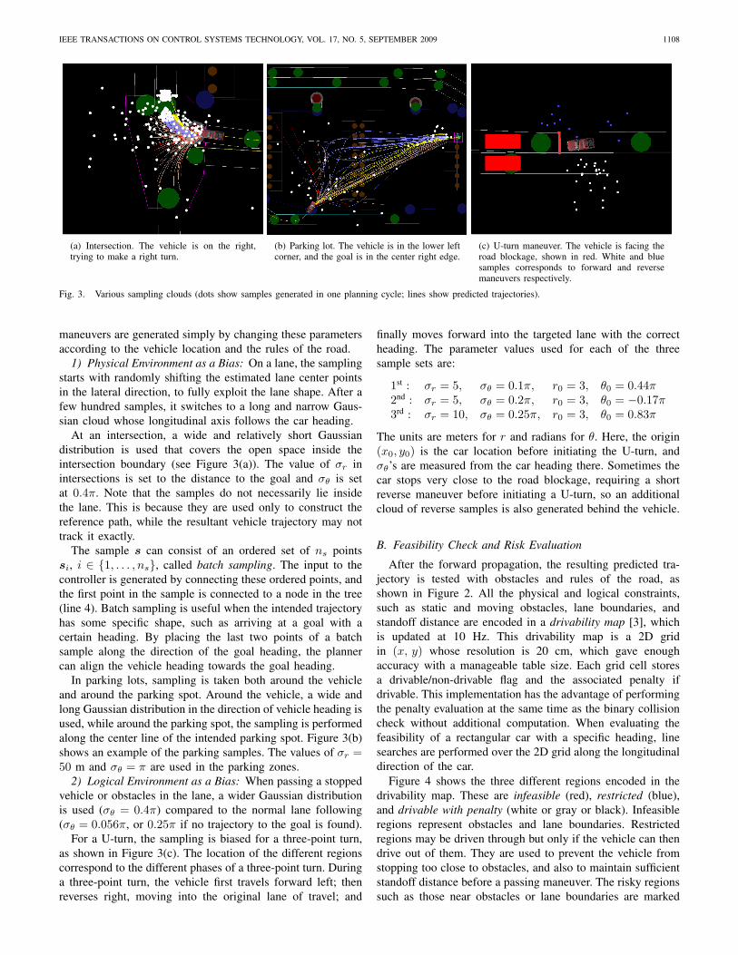
(a) Intersection. The vehicle is on the right,trying to make a right turn.

(b) Parking lot. The vehicle is in the lower leftcorner, and the goal is in the center right edge.

(c) U-turn maneuver. The vehicle is facing theroad blockage, shown in red. White and bluesamples corresponds to forward and reversemaneuvers respectively.

Fig. 3. Various sampling clouds (dots show samples generated in one planning cycle; lines show predicted trajectories).

maneuvers are generated simply by changing these parametersaccording to the vehicle location and the rules of the road.

1) Physical Environment as a Bias: On a lane, the samplingstarts with randomly shifting the estimated lane center pointsin the lateral direction, to fully exploit the lane shape. After afew hundred samples, it switches to a long and narrow Gaus-sian cloud whose longitudinal axis follows the car heading.

At an intersection, a wide and relatively short Gaussiandistribution is used that covers the open space inside theintersection boundary (see Figure 3(a)). The value of σr inintersections is set to the distance to the goal and σθ is setat 0.4π. Note that the samples do not necessarily lie insidethe lane. This is because they are used only to construct thereference path, while the resultant vehicle trajectory may nottrack it exactly.

The sample s can consist of an ordered set of ns pointssi, i ∈ {1, . . . , ns}, called batch sampling. The input to thecontroller is generated by connecting these ordered points, andthe first point in the sample is connected to a node in the tree(line 4). Batch sampling is useful when the intended trajectoryhas some specific shape, such as arriving at a goal with acertain heading. By placing the last two points of a batchsample along the direction of the goal heading, the plannercan align the vehicle heading towards the goal heading.

In parking lots, sampling is taken both around the vehicleand around the parking spot. Around the vehicle, a wide andlong Gaussian distribution in the direction of vehicle heading isused, while around the parking spot, the sampling is performedalong the center line of the intended parking spot. Figure 3(b)shows an example of the parking samples. The values of σr =50 m and σθ = π are used in the parking zones.

2) Logical Environment as a Bias: When passing a stoppedvehicle or obstacles in the lane, a wider Gaussian distributionis used (σθ = 0.4π) compared to the normal lane following(σθ = 0.056π, or 0.25π if no trajectory to the goal is found).

For a U-turn, the sampling is biased for a three-point turn,as shown in Figure 3(c). The location of the different regionscorrespond to the different phases of a three-point turn. Duringa three-point turn, the vehicle first travels forward left; thenreverses right, moving into the original lane of travel; and

finally moves forward into the targeted lane with the correctheading. The parameter values used for each of the threesample sets are:

1st : σr = 5, σθ = 0.1π, r0 = 3, θ0 = 0.44π2nd : σr = 5, σθ = 0.2π, r0 = 3, θ0 = −0.17π3rd : σr = 10, σθ = 0.25π, r0 = 3, θ0 = 0.83π

The units are meters for r and radians for θ. Here, the origin(x0, y0) is the car location before initiating the U-turn, andσθ’s are measured from the car heading there. Sometimes thecar stops very close to the road blockage, requiring a shortreverse maneuver before initiating a U-turn, so an additionalcloud of reverse samples is also generated behind the vehicle.

B. Feasibility Check and Risk Evaluation

After the forward propagation, the resulting predicted tra-jectory is tested with obstacles and rules of the road, asshown in Figure 2. All the physical and logical constraints,such as static and moving obstacles, lane boundaries, andstandoff distance are encoded in a drivability map [3], whichis updated at 10 Hz. This drivability map is a 2D gridin (x, y) whose resolution is 20 cm, which gave enoughaccuracy with a manageable table size. Each grid cell storesa drivable/non-drivable flag and the associated penalty ifdrivable. This implementation has the advantage of performingthe penalty evaluation at the same time as the binary collisioncheck without additional computation. When evaluating thefeasibility of a rectangular car with a specific heading, linesearches are performed over the 2D grid along the longitudinaldirection of the car.

Figure 4 shows the three different regions encoded in thedrivability map. These are infeasible (red), restricted (blue),and drivable with penalty (white or gray or black). Infeasibleregions represent obstacles and lane boundaries. Restrictedregions may be driven through but only if the vehicle can thendrive out of them. They are used to prevent the vehicle fromstopping too close to obstacles, and also to maintain sufficientstandoff distance before a passing maneuver. The risky regionssuch as those near obstacles or lane boundaries are marked


Fig. 4. Snapshot of the cost map.

as drivable with penalty. By adding the path integral of thepenalty to the time to traverse, the CL-RRT does not choosepaths that closely approach constraint boundaries, unless thereis no other option (e.g., narrow passage).

C. Node Connection Strategy

This subsection describe how the nodes in the tree are sortedon line 2 of Algorithm 1, when connecting a sample to thetree.

1) Distance Metric: RRT attempts to connect the sampleto the closest node in the tree. Because shorter paths havelower probability of collision, this approach requires minimumfunction calls for the computationally expensive collision de-tection [7]. RRT can thus quickly cover the free space withoutwasting many samples. Usually, the two-norm distance is usedto evaluate the “closeness”, but an extension is required whenRRT is applied to a vehicle with limited turning capability. Forexample, a car would need to make a big loop to reach a pointright next to the current location, due to the nonholonomicconstraints. The most accurate representation for this distancewould be the simulated trajectory of the vehicle as determinedby the propagation of the vehicle model. However, performinga propagation step for each node in the tree would impose aheavy computational burden. Thus the CL-RRT algorithm usesthe length of the Dubins path between a node and the sample.The use of Dubins path lengths has the advantage of capturingthe vehicle’s turning limitation with a simple evaluation of ananalytical solution. A full characterization of optimal Dubinspaths is given in [21] and a further classification in [22].

The node in the tree has a 2D position and a heading, andwithout loss of generality, it is assumed to be at the origin p0 =(0, 0, 0) ∈ SE(2), where SE(n) denotes a special Euclideangroup of dimension n. The sample is a 2D point representedby q = (x, y) ∈ R2. Since for the choice of p0, the Dubinspath lengths from p0 to the points (x, y) and (x, −y) areequal, it suffices to consider the case q = (x, |y|) ∈ R× R+.The minimum length Lρ(q) of a Dubins path from p0 to qcan be obtained analytically [23]. Let ρ denote the minimumturning radius of the vehicle. By defining Dρ = {z ∈ R2 :

‖z − (0, ρ)‖ < ρ}, the minimum length is given by

Lρ(q) = Lρ(q) =

{f(q) for q /∈ Dρ;g(q) otherwise,

where

f(q) =√d2

c (q)− ρ2 + ρ

(θc(q)− cos−1 ρ

dc(q)

),

g(q) = ρ

(α(q) + sin−1 x

df(q)− sin−1 ρ sin(α(q))

df(q)

),

and dc(q) =√x2 + (|y| − ρ)2 is the distance of q from the

point (0, ρ), θc(q) = atan2(x, ρ−|y|) is the angle of q from thepoint (0, ρ), measured counter-clockwise from the negative y-axis, df(q) =

√x2 + (|y|+ ρ)2 is the distance of q from the

point (0, −ρ), and α(q) = 2π − cos−1(

5ρ2−df(q)2

4ρ2

)is the

angular change of the second turn segment of the Dubins pathwhen q ∈ Dρ. Note that the atan2 function is the 4 quadrantinverse tangent function with atan2(a, b) = tan−1

(ab

), and its

range must be set to be [0, 2π) to give a valid distance. Thisanalytical calculation can be used to quickly evaluate all thenodes in the tree for a promising connection point.

2) Selection Criteria: Several heuristics have been pro-posed in the past [13], [24] to select the node to connectthe sample to. Because CL-RRT was designed to be usedin a constrained environment, it attempts multiple nodes insome order (∼ 10 in our implementation) before discardingthe sample. The following presents the heuristics used to sortthe nodes in the tree.

Before a trajectory to the goal is found, the tree is grownmainly according to an exploration heuristic, in which theemphasis of the algorithm is on adding new nodes to the treeto enlarge the space it covers. The nodes are sorted accordingto the Dubins distance Lρ(s), as presented above. Once afeasible trajectory to the goal has been found, the tree is grownprimarily according to an optimization heuristic. To make thenew trajectories progressively approach the shortest path, thenodes are now sorted in ascending order of total cost to reachthe sample. This total cost Ctotal is given by

Ctotal = Ccum(q) + Lρ(s)/v,

where Ccum(q) represents the cumulative cost from the root ofthe tree to a node q, v is the sampled speed, and the secondterm estimates the minimum time it takes to reach the samplefrom q.

Our experience has shown that, even before having atrajectory that reaches the goal and consequently when thefocus should be on exploration, some use of the optimizationheuristics is beneficial to reduce wavy trajectories. Similarly,once a feasible trajectory to the goal has been found andtherefore the focus should be on refining the available solution,some exploration of the environment is beneficial for examplein case an unexpected obstacle blocks the area around thefeasible solution, or for having a richer tree when the goallocation changes. Thus when implementing the algorithm, theratio of exploration vs. optimization heuristics used was 70%vs. 30% before a trajectory to the goal was found, and 30%vs. 70% after.


Note that stopping nodes in the tree are not considered aspotential connection points for the samples, unless it is theonly node of the tree or the driving direction changes. Thisprevents the vehicle from stopping for no reason and helpsachieve smooth driving behaviors.

D. Cost-To-Go Estimate

Every time a new node q is added to the tree, CL-RRTcomputes estimates of the cost-to-go from q to the goal(line 13–20). There are two estimates of the cost-to-go at eachnode in the tree, a lower bound and an upper bound. Thelower bound CLB is given by the Euclidean distance betweenthe vehicle position at the node and the position of the goal.The upper bound CUB is obtained differently from [13], whichassumed the existence of the optimal control policy.

For each newly added node q, a trajectory from q to thegoal is generated and evaluated for feasibility. If it is collision-free, the cost associated with that trajectory gives the upperbound CUB at q. This upper bound is then propagated fromq backward towards the root to see if it gives a better upperbound from ancestor nodes of q. Thus, CUB is given by

CUB =

∞ : no trajectory to the goal availableminc

(ec + CUBc) : trajectory to the goal available

CLB : node is inside the goal region

where c represents the index of each child of this node, ec isthe cost from the node to the child node c, and CUBc representsthe upper bound cost at node c.

Note that this process adds a node at the goal to the treeif the goal is directly reachable from q, which helps CL-RRTquickly find a trajectory to reach the goal in most scenarios.As time progresses, more trajectories that reach the goal areconstantly added to the tree.

These cost estimates are used when choosing the best tra-jectory to execute (as shown later on line 13 of Algorithm 2).Once a feasible trajectory to the goal is found, the bestsequence of nodes is selected based on the upper bound CUB.Before a goal-reaching trajectory is found, the node with thebest lower bound is selected, in effect trying to move towardsthe goal as much as possible.

E. Safety as an Invariant Property

1) Safe States: Ensuring the safety of the vehicle is animportant feature of any planning system, especially when thevehicle operates in a dynamic and uncertain environment. Wedefine a state x(t0) to be safe if the vehicle can remain in thatstate for an indefinite period of time

x(t0) = 0, x(t0) ∈ Xfree(t) ∀t ≥ t0

without violating the rules of the road and at the sametime is not in a collision state/path with stationary and/ormoving obstacles – where the latter are assumed to maintaintheir current driving path. A complete stop is used as safestate in this paper. More general notions of safe states areavailable [13], [25]. The large circles in Figure 2 show thesafe stopping nodes in the tree. Given a reference path (shown

Algorithm 2 Execution loop of RRT.1: repeat2: Update the current vehicle states x0 and environmental

constraints Xfree(t)3: Propagate the states by the computation time and obtain

x(t0 + ∆t)4: repeat5: Expand tree()6: until time limit ∆t is reached7: Choose the best safe node sequence in the tree8: if No such sequence exists then9: Send E-Stop to controller and goto line 2

10: end if11: Repropagate from the latest states x(t0 +∆t) using the

r associated with the best node sequence, and obtainx(t), t ∈ [t1, t2]

12: if x(t) ∈ Xfree(t)∀t ∈ [t1, t2] then13: Send the best reference path r to controller14: else15: Remove the infeasible portion and its children from

the tree, and goto line 716: end if17: until the vehicle reaches goal

with orange), a speed profile is designed in such a way thatthe vehicle comes to a stop at the end. Then, each forwardsimulation terminates when the vehicle comes to a stop. Byrequiring that all leaves in the tree are safe states, this approachguarantees that there is always a feasible way to come to a stopwhile the car is moving. Unless there is a safe stopping nodeat the end of the path, the vehicle does not start executing it.With stopping nodes at the leaves of the tree, some behaviorssuch as stopping at a stop line emerge naturally.

2) Unsafe Node: A critical difference from previouswork [13] is the introduction of “unsafe” nodes. In [13],when the propagated trajectory is not collision-free, the entiretrajectory is discarded. In our approach, when only the finalportion of the propagated trajectory is infeasible, the feasibleportion of the trajectory is added to the tree. This avoidswasting the computational effort required to find a goodsample, propagate, and check for collision, while retaining thepossibility to execute the portion that is found to be feasible.Because this trajectory does not end in a stopped state, thenewly added nodes are marked as “unsafe”. When a safetrajectory ending in a stopped state is added to the unsafenode, the node is marked as safe. This approach uses unsafenodes as potential connection points for samples, increasingthe density of the tree, while ensuring the safety of the vehicle.

V. ONLINE REPLANNING

In a dynamic and uncertain environment, the tree needs tokeep growing during the execution because of the constantupdate of the situational awareness. Furthermore, real-timeexecution requirements necessitate reuse of the informationfrom the previous computation cycle [26]–[28].

Algorithm 2 shows how CL-RRT executes a part of the treeand continues growing the tree while the controller executes


the plan. The planner sends the input to the controller r at afixed rate of every ∆t seconds. The tree expansion continuesuntil a time limit is reached (line 6). The best trajectory isselected and the reference path is sent to the controller forexecution (line 13). The expansion of the tree is resumed afterupdating the vehicle states and the environment (line 2).

Note that when selecting the best trajectory on line 7, onlythe node sequences that end in a safe state are considered. Ifnone is found, then the planner will command an emergencybraking maneuver to the controller in order to bring the car toa stop as fast as possible.

A. Committed part of the tree

A naive way to implement an RRT-based planner is to builda new tree (discarding the old) at every planning cycle, andselect the plan for execution independent of the plan currentlybeing executed. If the tree from the previous planning cycleis discarded, almost identical computations would have to berepeated. In a real-time application with limited computing re-sources, such an inefficiency could result in a relatively sparsetree as compared to the case where available computationare used to add new feasible trajectories to the existing tree.Furthermore, if the tree is discarded every cycle and hencethe plan for execution is selected independently of the planbeing executed, the planner could switch between differenttrajectories of marginally close cost/utility at every planningcycle, potentially resulting in wavy trajectories.

To address these issues, the CL-RRT algorithm maintains a“committed” trajectory, the end of which coincides with theroot node. After the first planning cycle, a feasible plan is sentto the controller for execution. The portion from the root tothe next node is marked as committed. For the next planningcycle, this node is initialized as the new root node, and all otherchildren branches from the old root are then deleted becausethese branches will never be executed. The tree growing phasewill then proceed with all subsequent trajectories originatingfrom this new root node. When the propagated vehicle statesx(t0 + ∆t) (line 3) reach the end of the committed trajectory,the best child node of the root is initialized as the new root,and all other children are deleted. Therefore, the vehicle isalways moving towards the root of the tree.

This approach ensures that the tree is maintained from theprevious planning cycle, and that the plan that the controlleris executing (corresponding to the committed part of the tree)is always continuous. Because the planner does not changeits decision over the committed portion, it is important notto commit a long trajectory especially in a dynamic and un-certain environment. The CL-RRT ensures that the committedtrajectory is not longer than 1 m, by adding branch points ifthe best child of the root is farther than that distance.

B. Lazy Reevaluation

In a dynamic and uncertain environment, the feasibilityof each trajectory stored in the tree should be re-checkedwhenever the perceived environment is updated. A large tree,however, could require constant reevaluation of its thousandsof edges, reducing the time available for growing the tree.

Input to controllerPredicted pathActual pathRepropagationCurrent

states

Best path

StartGoal

Obstacle

Fig. 5. Repropagation from the current states.

The approach introduced in this paper to overcome this issuewas to reevaluate the feasibility of a certain edge only whenit is selected as the best trajectory sequence to be executed. Ifthe best trajectory is found infeasible, the infeasible portion ofthe tree is deleted and the next best sequence is selected forreevaluation. This “lazy reevaluation” enables the algorithmto focus mainly on growing the tree, while ensuring that theexecuted trajectory is always feasible with respect to the latestperceived environment. The primary difference from previouswork [29], [30] is that the lazy check in this paper is aboutre-checking of the constraints for previously feasible edges,whereas the previous work is about delaying the first collisiondetection in the static environment.

C. Repropagation

Although the feedback loop embedded in the closed-loopprediction can reduce the prediction error, the state predictioncould still have non-zero errors due to inherent modelingerrors or disturbances. To address the prediction error, onecan discard the entire tree and rebuild it from the latest states.However, this is undesirable as highlighted in Section V-A.

The CL-RRT algorithm reuses the controller inputs stored inthe tree and performs a repropagation from the latest vehiclestates, as shown in Figure 5. With a stabilizing controller, thedifference between the original prediction and the repropa-gation would converge to zero if the reference path has asufficiently long straight line segment.

Instead of repropagating over the entire tree, the CL-RRTalgorithm repropagates from the latest states only along thebest sequence of nodes (line 11 of Algorithm 1). If the reprop-agated trajectory is collision free, the corresponding controllerinput is sent to the controller. Otherwise, the infeasible partof the tree is deleted from the tree, and the next best nodesequence is selected and repropagated. This approach requiresonly a few reevaluations of the edge feasibility, while ensuringthe feasibility of the plan being executed regardless of theprediction errors.


(a) Forward Drive (b) Reverse Drive

Fig. 6. Definition of pure-pursuit variables. Two shaded rectangles representthe rear tire and the steerable front tire in the bicycle model. The steeringangle in this figure, δ, corresponds to negative δ in Eq. (4).

VI. IMPLEMENTATION OF THE CONTROLLER

CL-RRT uses the controller in two different ways. One isin the closed-loop prediction together with the vehicle model,and the other is in the execution of the motion plan in realtime. In our implementation, the controller ran at 25 Hz in theexecution, and the same time step size was used in the closed-loop simulation. The same controller code was used for bothexecution and prediction.

A. Steering Controller

The steering controller is based on the pure-pursuit con-troller, which is a nonlinear path follower that has been widelyused in ground robots [31] and more recently in unmanned airvehicles [32]. It is adopted due to its simplicity, as an intuitivecontrol law that has a clear geometric meaning. Because theDUC rules restrict the operating speed to be under 30 mph andextreme maneuvers (e.g., high speed tight turns) are avoided,dynamic effects such as side slip are neglected for controldesign purposes.

The kinematic bicycle model is described by

x = v cos θ, y = v sin θ, θ =v

Ltan δ (4)

where, x and y refer to the rear axle position, θ is thevehicle heading with respect to the x-axis (positive counter-clockwise), v is the forward speed, δ is the steer angle (positivecounter-clockwise), and L is the vehicle wheelbase. Withthe slip-free assumption, Figure 6(a) shows the definition ofthe variables that define the pure-pursuit control law whendriving forwards, and Figure 6(b) shows the variables whendriving in reverse. Here, R is the radius of curvature, and“ref path” is the piecewise linear reference path given bythe planner. In Figure 6(a), lfw is the distance of the forwardanchor point from the rear axle, Lfw is the forward drive look-ahead distance, and η is the heading of the look-ahead point(constrained to lie on the reference path) from the forwardanchor point with respect to the vehicle heading. Similarly, inFigure 6(b), lrv is the rearward distance of the reverse anchorpoint from the rear axle, Lrv is the reverse drive look-aheaddistance, and η is the heading of the look-ahead point fromthe reverse anchor point with respect to the vehicle headingoffset by π rad. All angles and lengths shown in Figure 6 arepositive by definition.

Using elementary planar geometry, the instantaneous steerangles required to put the anchor point on a collision coursewith the look-ahead point can be computed as

δ = − tan−1

(L sin η

Lfw2 + lfw cos η

): forward drive

δ = − tan−1

(L sin η

Lrv2 + lrv cos η

): reverse drive

which gives the modified pure-pursuit control law. Note thatby setting lfw = 0 and lrv = 0, the anchor points coincidewith the rear axle, recovering the conventional pure-pursuitcontroller [31].

A stability analysis of this controller has been carried outin Ref. [15]. It approximates the slew rate limitation of thesteering actuation with a first order system of time constant τ ,showing that Lfw > vτ − lfw and Lrv > −vτ − lrv for HurwitzStability. This means that in a high velocity regime, largerLfw is required for stability. Some margin should be addedto account for disturbances and modeling error. However,too large Lfw degrades the tracking performance. Throughextensive simulations and field tests, the following numberswere selected

Lfw(vcmd) =

3 if vcmd < 1.34,2.24 vcmd if 1.34 ≤ vcmd < 5.36,12 otherwise.

with τ = 0.717. The same rule is also employed for backwarddriving, i.e., Lfw(vcmd) = Lrv(vcmd). From this point on,L1 represents the look-ahead distance Lfw and Lrv. For thereason elaborated in Subsection VI-C1, L1 is scaled with thecommanded speed vcmd and not the actual speed v.

B. Speed ControllerFor speed tracking, a simple Proportional-Integral-

Derivative (PID) type controller is considered. However, ourassessment is that the PID controller offers no significantadvantage over the PI controller because the vehicle hassome inherent speed damping and the acceleration signalrequired for PID control is noisy. Hence, the PI controller ofthe following form is adopted

u = Kp (vcmd − v) +Ki

∫ t

0

(vcmd − v) dτ

where u is the non-dimensional speed control signal, Kp andKi are the proportional and integral gain respectively.

The controller coefficients Kp and Ki were determinedby extensive testing guided by the parameter space approachof robust control [33]. Given certain design specifications interms of relative stability, phase margin limits, and robustsensitivity; using the parameter space approach, it is possibleto enclose a region in the Kp − Ki plane for which thedesign specifications are satisfied. Then, via actual testing,controller parameters within this region that best fit the ap-plication was identified. As detailed more in [15], consideringa low-bandwidth noise-averse control design specification, thefollowing gains have been selected

Kp = 0.2, Ki = 0.04.


C. Accounting for the Prediction ErrorWhen the controller does not track the reference path

perfectly due to modeling errors or disturbances, the plan-ner could adjust the reference command so that the vehicleachieves the original desired path. However, it introduces anadditional feedback loop, potentially destabilizing the overallsystem. When both the planner and the controller try to correctfor the same error, they could be overcompensating or negatingthe effects of the other.

In our approach, the planner generates a “large” signal inthe form of the reference path, but it does not adjust the pathdue to the tracking error. It is controller’s responsibility totrack the path in a “small” signal sense. Thus, the propagationof trajectories (line 5 of Algorithm 2) starts from the predictedvehicle states at the node. One challenge here is that thecollision is checked with the predicted trajectory, which canbe as long as several seconds. Although Subsection V-Caddressed the case when the prediction error becomes large,it is still critical to keep the prediction error small in orderto have acceptable performance. This section presents severaltechniques to reduce prediction errors.

1) Use of vcmd for L1 scheduling: As discussed in Sec-tion VI-A, the look-ahead distance L1 must increase withthe vehicle speed to maintain stability. However, schedulingL1 based on the speed v means that any prediction error inthe speed directly translates into a discrepancy of the steercommand between prediction and execution, introducing alateral prediction error. This is problematic because achievinga small speed prediction error is very challenging especiallyduring the transient in the low-speed regime, where the enginedynamics and gear shifting of the automatic transmissionexhibits complicated nonlinearities. Another disadvantage ofscaling L1 with v is that the noise in the speed estimateintroduces jitters in the steering command.

A solution to this problem is to use the speed command vcmdto schedule the L1 distance. The speed command is designedby the planner, uncorrupted by noise or disturbances, so theplanner and controller have the same vcmd with no ambiguity.Then, the same steering gain L1 is used in the prediction andexecution, rendering the steering prediction decoupled fromthe speed prediction.

2) Space-dependent speed command: In Section III, thereference command r was defined as a function of time.For the speed command vcmd, however, it is advantageous toassociate it to the position of the vehicle.

When the speed command is defined as a function of time,the prediction error in the speed could affect the steeringperformance, even if the look-ahead distance L1 is scaledbased on vcmd. Suppose the vehicle accelerates from rest witha ramp command. If the actual vehicle accelerates more slowlythan predicted, the time-based vcmd would increase faster thanthe prediction with respect to the travel distance. This meansthat L1 increases more in the execution before the vehiclemoves much, and given a vehicle location, the controllerplaces a look-ahead point farther down on the reference pathcompared to prediction.

To overcome this issue, the speed command is associatedwith the position of the vehicle with respect to the predicted

path. Then, the steering command depends only on where thevehicle is, and is insensitive to speed prediction errors.

VII. APPLICATION RESULTS

This section presents the application results of CL-RRTalgorithm on MIT’s DUC entry vehicle, Talos.

A. Vehicle Model

The following nonlinear model is used in the prediction.

x = v cos θ y = v sin θ

θ =v

Ltan δ ·Gss δ =

1Td

(δc − δ)

v = a a =1Ta

(ac − a)

amin ≤ a ≤ amax

‖δ‖ ≤ δmax ‖δ‖ ≤ δmax

The inputs to this system are the steering angle command δcand the longitudinal acceleration command ac. These inputsgo through a first-order lag with time constants Td and Tafor the steering and acceleration respectively. The maximumsteering angle is given by δmax, and the maximum slew ratefor the steering is δmax. The forward acceleration is denotedby a, with the bounds of maximum deceleration amin andmaximum acceleration amax.

The term Gss, which did not appear in Eq. (4), captures theeffect of side slip

Gss =1

1 + (v/vCH)2

and is a static gain of the yaw rate θ, i.e. the resulting yaw ratewhen the derivative of the side-slip angle and the derivativeof yaw rate are both zero [33]. The parameter vCH is calledthe characteristic velocity [33], [34] and can be determinedexperimentally. This side slip model has several advantages: itdoes not increase the model order, and hence the computationrequired for propagation; the model behaves the same as thekinematic model in the low speed regime; and it requires onlyone parameter to tune. Moreover, this model does not differmuch from the nonlinear single track model [33] for the urbandriving conditions where extreme maneuvers are avoided andup to 30 mph speeds are considered.

The following parameters were used for Talos, a 4.9-meter-long and 2.0-meter-wide Land Lover LR3.

δmax = 0.5435 rad δmax = 0.3294 rad/sTd = 0.3 s Ta = 0.3 s

amin = −6.0 m/s2 amax = 1.8 m/s2

L = 2.885 m vCH = 20.0 m/s

From the parameters above, the minimum turning radius isfound to be 4.77 m.


Fig. 7. Lane following on a high speed curvy section. The vehicle speed is10 m/s. The green dots show the safe stopping nodes in the tree.

0 20 40 60 80 100 120 140−5

0

5

10

15

t (s)

v(m

/s)

vcmd

vvmax

0 20 40 60 80 100 120 140−0.2

0

0.2

0.4

0.6

t (s)

e lat

(m)

Fig. 8. Prediction error during this segment

B. Race Results

The following subsections present results from the NationalQualification Event (NQE) and the final Urban ChallengeEvent (UCE). NQE consisted of three test areas A, B, and C,each focusing on testing different capabilities. During NQE,the CL-RRT algorithm was not tuned to any specific test area,showing the generality of the approach. UCE consisted of threemissions, with a total length of about 60 miles. Talos was oneof the six vehicles that completed all missions, finishing in 5hours 35 minutes.

In Talos, the motion planner was executed on a dual-core2.33 GHz Intel Xeon processor at approximately 10 Hz. Thetime limit ∆t in Algorithm 2 is 0.1 second and the algorithmuses 100% CPU by design. The average number of samplesgenerated was approximately 700 samples per second and thetree had about 1200 nodes on average. Notice that becausethe controller input is the parameter that is sampled, a singlesample could create a trajectory as long as several seconds.

1) High speed behavior on a curvy road: Figure 7 showsa snapshot of the environment and the plan during UCE.The vehicle is in the lower left, going towards a goal inthe upper middle of the figure. The small green squares

Fig. 9. Tree consisting of many unsafe nodes in the merge test.

represent the safe stopping nodes in the tree. The vehicleis moving at 10 m/s, so there are no stopping nodes in theclose range. However, the planner ensures there are numerousstopping points on the way to the goal, should intermittentlydetected curbs or vehicles appear. Observe that even though thecontroller inputs are randomly generated to build the tree, theresulting trajectories naturally follow the curvy road. This roadsegment is about 0.5 mile long, and the speed limit specifiedby DARPA was 25 mph. Figure 8 shows the speed profileand the lateral prediction error for this segment. Talos reachedthe maximum speed several times on straight segments, whileslowing down on curvy roads to observe the maximum lateralacceleration constraints. The prediction versus execution errorhas the mean, maximum, and standard deviation of 0.11 m,0.42 m, and 0.093 m respectively. Note from the plot that theprediction error has a constant offset of about 11 cm, makingthe maximum error much larger than the standard deviation.This is due to the fact that the steering wheel was not perfectlycentered and the pure-pursuit algorithm does not have anyintegral action to remove the steady state error.

Note that when the prediction error happens to becomelarge, the planner does not explicitly minimize it. This occursbecause the vehicle keeps executing the same plan as long asthe repropagated trajectory is feasible. In such a scenario, theprediction error could grow momentarily. For example, duringa turn with a maximum steering angle, a small differencebetween the predicted initial heading and the actual headingcan lead to a relatively large error as the vehicle turns. Evenwith a large mismatch, however, the repropagation process inSection V-C ensures the safety of the future path from vehicle’scurrent state.

2) Unsafe Nodes in the Dynamic Environment: Figure 9is a snapshot from the merging test in NQE. Talos is in thebottom of the figure, trying to turn left into the lane and mergeinto the traffic. The red lines originating from Talos show theunsafe trajectories, which do not end in a stopped state.

Before the traffic vehicle comes close to the intersection,there were many trajectories that reach the goal. However, asthe traffic vehicle (marked with a green rectangle) approached,its path propagated into the future blocks the goal of Talos,as shown in Figure 9, which rendered the end parts ofthese trajectories infeasible. However, the feasible portion ofthese trajectories remain in the tree as unsafe nodes (see


t0, t1HHY

t2�

�

t3��

t4��9

t5�

t0

6

t1BBBN

t2

?

t3 -

Fig. 12. Sequence of events. Talos (maroon) remains stationary between t0and t1, and Odin (white) had progressed beyond the view window by t4.

Section IV-E2), from which the tree is quickly grown to thegoal once the traffic vehicle leaves the intersection.

3) Parking: Figure 10 shows Talos’ parking maneuverinside the zone during NQE. Figure 10(a) shows a super-imposed sequence of Talos’ pose for the parking maneuver.Figure 10(b) shows a tree of trajectories before going intothe parking spot. The purple lines show forward trajectoriesreaching the goal; the light brown lines show forward trajec-tories that do not reach the goal; the turquoise lines showreverse trajectories; and the red lines show unsafe trajectories.The motion plan is marked with two colors: the orange lineis the input to the steering controller; and the green lineis the predicted trajectory on which the speed command isassociated.

In Figure 10(c), Talos is reversing to go out of the spot andintends to exit the parking zone. The goal for the planner isnow at the exit of the zone located in the upper right cornerof the figure, and there are many trajectories that go towardsit. Following the plan selected from these trajectories, Talossuccessfully exited the parking zone.

4) Road Blockage: Figure 11 shows the behavior of Talosduring a U-turn that was required in the Area C test. Themotion planner always tries to make forward progress, butafter 50 seconds of no progress, the Navigator declares ablockage and places the goal in the lane with the oppositetravel direction. Figure 11(a) shows a sequence of Talos’spose during the maneuver. The road to the right is blockedby a number of traffic barrels. In Figure 11(b), it can beseen that there are several trajectories reaching the goal inthe destination lane. Figure 11(c) shows the last segment ofthe U-turn. Because of the newly detected curbs in front ofthe vehicle, the maneuverable space has becomes smaller thanin (b), resulting in a 5-pt turn.

5) Interaction with Virginia Tech’s Odin: Figures 12 and 13show an interaction that occurred between Talos and VirginiaTech’s Odin in the UCE, with the main result being that Talos

took an evasive swerving maneuver to avoid a collision.Initially, Talos arrived at the intersection and stopped at

the stop line (Figure 13(a)). Odin is approaching the inter-section from the left, and its predicted trajectory goes into theintersection. Although Odin did not have a stop line on itslane, it stopped when it reached the intersection and remainedmotionless for about 3 seconds. With the intersection clear,and all vehicles stopped, Talos assumed precedence over Odinand started driving through the intersection (Figure 13(b)). Justas Talos started, however, Odin also started driving, headingtowards the same lane that Talos was heading, and blockedTalos’ path (Figure 13(c)). Talos took an evasive maneuver toavoid collision and stop safely by steering left and applyingstrong brake (white circle around Talos). Odin continued alongits path, and once it (and the trailing human-occupied DARPAchase vehicle) cleared the intersection, Talos recomputes a newplan and proceeds through the intersection (Figure 13(d)).

This is just one example of the numerous traffic andintersection scenarios that had never been tested before therace, and yet the motion planner demonstrated that it wascapable of handling these situations safely. While Talos hasdemonstrated that it is generally operating safely even inuntested scenarios, it was nonetheless involved in two crashincidents during the UCE [3]. However, the analysis in [35]indicates that the primary contributing factor in those twoinstances was an inability to accurately detect slow movingvehicles.

6) Repropagation: Most of the time during the race, thetrajectory repropagated from the latest states and the trajectorystored in the tree are close. However, there are some instanceswhen the repropagation resulted in a different trajectory. InFigure 13(d), Talos slowed down more than the prediction,so the trajectory repropagated from the latest states (the pinkline shown with an arrow in the figure) is a little off fromthe trajectories stored in the tree. However, as long as therepropagation is feasible, Talos keeps executing the samecontroller input. This approach is much more efficient thandiscarding the tree when the prediction error exceeds anartificial limit and rebuilding the tree.

VIII. CONCLUSION

This paper presented the CL-RRT algorithm, a sampling-based motion planning algorithm specifically developed forlarge robotic vehicles with complex dynamics and operatingin uncertain, dynamic environments such as urban areas. Thealgorithm was implemented as the motion planner for Talos,the autonomous Land Rover LR3 that was MIT’s entry in the2007 DARPA Urban Challenge.

The primary novelty is the use of closed-loop predictionin the framework of RRT. The combination of stabilizingcontroller and forward simulation has enabled application ofCL-RRT to vehicles with complex, nonlinear, and unstabledynamics. Several extensions are presented regarding RRT treeexpansion: a simple sampling bias strategy to generate variousdifferent maneuvers; penalty value in addition to the binarycheck of edge feasibility; use of Dubins path length whenselecting the node to connect; and guaranteed safety even when


(a) Overall trajectory of Talos. (b) Going towards the parking spot. (c) After parked, Talos reversing to its left and goingto the exit.

Fig. 10. Parking maneuver in the parking zone in an Area B test.

(a) Overall trajectory of Talos. (b) Talos initiated first segment of U-turn. (c) Talos starting last segment of U-turn.

Fig. 11. U-turn maneuver at a blocked road in an Area C test.

the vehicle is in motion. By retaining the tree during execu-tion, the CL-RRT reuses the information from the previouscomputation cycle, which is important especially in real-timeapplications. The extensions made to online replanning includethe lazy reevaluation to account for changing environments andthe repropagation to account for prediction errors.

The advantages of the CL-RRT algorithm were demon-strated through the race results from DUC. The successfulcompletion of the race with numerous differing scenarios usingthis single planning algorithm demonstrates the generality andflexibility of the CL-RRT planning algorithm.

ACKNOWLEDGMENT

Research was sponsored by Defense Advanced ResearchProjects Agency, Program: Urban Challenge, DARPA OrderNo. W369/00, Program Code: DIRO. Issued by DARPA/CMOunder Contract No. HR0011-06-C-0149, with Prof. JohnLeonard, Prof. Seth Teller, Prof. Jonathan How at MIT andProf. David Barrett at Olin College as the principal investi-gators. The authors gratefully acknowledge the support of theMIT DARPA Urban Challenge Team, with particular thanksto Dr. Luke Fletcher and Dr. Edwin Olson for their develop-ment of the drivability map, David Moore for developing theNavigator, Dr. Karl Iagnemma for his expert advice, StefanCampbell for his initial design and implementation of thecontroller, and Steven Peters for his technical support duringthe development of Team MIT’s vehicle.

REFERENCES

[1] K. Iagnemma and M. Buehler, eds., “Special issue on the DARPA grandchallenge, part 1,” Journal of Field Robotics, vol. 23, no. 8, pp. 461–652,Aug. 2006.

[2] ——, “Special issue on the 2007 DARPA urban challenge,” Journal ofField Robotics, vol. 25, pp. 423–860, 2008.

[3] J. Leonard, J. How, S. Teller, M. Berger, S. Campbell, G. Fiore,L. Fletcher, E. Frazzoli, A. Huang, S. Karaman, O. Koch, Y. Kuwata,D. Moore, E. Olson, S. Peters, J. Teo, R. Truax, M. Walter, D. Barrett,A. Epstein, K. Maheloni, K. Moyer, T. Jones, R. Buckley, M. Antone,R. Galejs, S. Krishnamurthy, and J. Williams, “A perception drivenautonomous urban vehicle,” Journal of Field Robotics, vol. 25, no. 10,pp. 727–774, 2008.

[4] J.-C. Latombe, Robot Motion Planning. Boston, MA: Kluwer, 1991.[5] J.-P. Laumond, Ed., Robot Motion Planning and Con-

trol. Berlin: Springer-Verlag, 1998, available online athttp://www.laas.fr/˜jpl/book.html.

[6] H. Choset, K. M. Lynch, S. Hutchinson, G. Kantor, W. Burgard, L. E.Kavraki, and S. Thrun, Principles of Robot Motion: Theory, Algorithms,and Implementations. Cambridge, MA: MIT Press, 2005.

[7] S. M. LaValle, Planning Algorithms. Cambridge, U.K.: CambridgeUniversity Press, 2006, available at http://planning.cs.uiuc.edu/.

[8] K. Iagnemma and M. Buehler, eds., “Special issue: Special issue on theDARPA grand challenge, part 2,” Journal of Field Robotics, vol. 23,no. 9, pp. 655–835, Sept. 2006.

[9] S. M. LaValle and J. J. Kuffner, “Randomized kinodynamic planning,”in Proceedings IEEE International Conference on Robotics and Automa-tion, 1999, pp. 473–479.

[10] ——, “Randomized kinodynamic planning,” International Journal ofRobotics Research, vol. 20, no. 5, pp. 378–400, May 2001.

[11] ——, “Rapidly-exploring random trees: Progress and prospects,” inAlgorithmic and Computational Robotics: New Directions, B. R. Donald,K. M. Lynch, and D. Rus, Eds. Wellesley, MA: A K Peters, 2001, pp.293–308.


(a) Odin approaches the intersection, Talos stopped at t0. (b) Odin stops at intersection, Talos starts maneuver at t1.

(c) Odin moves into intersection, Talos detected potential collision andexecutes avoidance maneuver at t2.

(d) Odin clears intersection, Talos proceeds through intersection at t3.

Fig. 13. Talos successfully avoids Virginia Tech’s Odin at an intersection.

[12] D. Hsu, J.-C. Latombe, and R. Motwani, “Path planning in expansiveconfiguration spaces,” International Journal Computational Geometry &Applications, vol. 4, pp. 495–512, 1999.

[13] E. Frazzoli, M. A. Dahleh, and E. Feron, “Real-time motion planningfor agile autonomous vehicles,” AIAA Journal of Guidance and Control,vol. 25, no. 1, pp. 116–129, 2002.

[14] T. Howard and A. Kelly, “Optimal rough terrain trajectory generationfor wheeled mobile robots,” International Journal of Robotics Research,vol. 26, no. 2, pp. 141–166, 2007.

[15] Y. Kuwata, J. Teo, S. Karaman, G. Fiore, E. Frazzoli, and J. P.How, “Motion planning in complex environments using closed-loopprediction,” in AIAA Guidance, Navigation and Control Conference andExhibit, Honolulu, HI, Aug. 2008, AIAA–2008–7166.

[16] S. R. Lindemann and S. M. LaValle, “Incrementally reducing dispersionby increasing Voronoi bias in RRTs,” in Proceedings IEEE InternationalConference on Robotics and Automation, 2004.

[17] ——, “Steps toward derandomizing RRTs,” in IEEE Fourth Interna-tional Workshop on Robot Motion and Control, 2004.

[18] M. Strandberg, “Augmenting RRT-planners with local trees,” in Proceed-ings IEEE International Conference on Robotics & Automation, 2004,pp. 3258–3262.

[19] C. Urmson and R. Simmons, “Approaches for heuristically biasingRRT growth,” in Proceedings IEEE/RSJ International Conference onIntelligent Robots and Systems, 2003.

[20] A. Yershova, L. Jaillet, T. Simeon, and S. M. LaValle, “Dynamic-domainRRTs: Efficient exploration by controlling the sampling domain,” in Pro-ceedings IEEE International Conference on Robotics and Automation,2005.

[21] L. E. Dubins, “On curves of minimal length with a constraint on

average curvature, and with prescribed initial and terminal positions andtangents,” American Journal of Mathematics, vol. 79, pp. 497–516, 1957.

[22] A. M. Shkel and V. Lumelsky, “Classification of the dubins set,”Robotics and Autonomous Systems, vol. 34, pp. 179–202, Mar. 2001.

[23] J. J. Enright, E. Frazzoli, K. Savla, and F. Bullo, “On multiple uavrouting with stochastic targets: Performance bounds and algorithms,” inProceedings AIAA Guidance, Navigation, and Control Conference andExhibit, Aug. 2005.

[24] P. Indyk, “Nearest neighbors in high-dimensional spaces,” in Handbookof Discrete and Computational Geometry, 2nd Ed., J. E. Goodman andJ. O’Rourke, Eds. New York: Chapman and Hall/CRC Press, 2004,pp. 877–892.

[25] T. Schouwenaars, J. How, and E. Feron, “Receding horizon path plan-ning with implicit safety guarantees,” in Proceedings American ControlConference, vol. 6, June 2004.

[26] A. Stentz, “Optimal and efficient path planning for partially-known en-vironments,” in Proceedings IEEE International Conference on Robotics& Automation, 1994, pp. 3310–3317.

[27] S. Petti and T. Fraichard, “Safe motion planning in dynamic environ-ments,” in Proceedings IEEE International Conference on Robotics &Automation, 2005.

[28] M. Zucker, J. Kuffner, and M. Branicky, “Multipartite RRTs for rapidreplanning in dynamic environments,” in Proc. IEEE Int. Conf. Roboticsand Automation, 2007.

[29] R. Bohlin and L. Kavraki, “Path planning using Lazy PRM,” in Proceed-ings IEEE International Conference on Robotics & Automation, 2000.

[30] G. Sanchez and J.-C. Latombe, “A single-query bi-directional proba-bilistic roadmap planner with lazy collision checking,” in ProceedingsInternational Symposium on Robotics Research, 2001.


[31] O. Amidi and C. Thorpe, “Integrated Mobile Robot Control,” in Pro-ceedings of SPIE, W. H. Chun and W. J. Wolfe, Eds., vol. 1388. Boston,MA: SPIE, Mar. 1991, pp. 504–523.

[32] S. Park, J. Deyst, and J. P. How, “Performance and Lyapunov Stabilityof a Nonlinear Path-Following Guidance Method,” Journal of Guidance,Control, and Dynamics, vol. 30, no. 6, pp. 1718–1728, Nov. 2007.

[33] J. Ackermann, Robust Control: The Parameter Space Approach.Springer, 2002.

[34] T. N. Gillespie, Fundamentals of Vehicle Dynamics. Warrendale, PA:Society of Automotive Engineers, 1992.

[35] L. Fletcher, S. Teller, E. Olson, D. Moore, Y. Kuwata, J. How, J. Leonard,I. Miller, M. Campbell, D. Huttenlocher, A. Nathan, and F.-R. Kline,“The MIT – Cornel collision and why it happened,” Journal of FieldRobotics, vol. 25, no. 10, pp. 775–807, 2008.

Yoshiaki Kuwata received the B.Eng degree fromthe University of Tokyo in 2001, and the S.M.and Ph.D. degrees in Aeronautics and Astronauticsfrom Massachusetts Institute of Technology (MIT) in2003 and 2007, respectively. In 2007, he worked onthe DARPA Urban Challenge as a postdoctoral as-sociate at MIT. He then joined the Robotics Sectionof Jet Propulsion Laboratory, California Institute ofTechnology in 2008. His current research interestsinclude cooperative control, vision-based guidance,and path planning for unmanned aerial/ground/sea-

surface vehicles.

Justin Teo received the B.Eng degree from NanyangTechnological University, Singapore, in 1999, andthe M.Sc degree from National University of Sin-gapore in 2003. He joined DSO National Labora-tories, Singapore, in 1999. Since 2005, DSO Na-tional Laboratories has funded his Ph.D. studies inthe Department of Aeronautics and Astronautics,Massachusetts Institute of Technology. His researchinterests include nonlinear control, adaptive control,and trajectory planning.

Gaston Fiore received the B.S. degree in AerospaceEngineering with Information Technology and anM.S. degree in Aeronautics and Astronautics, bothfrom the Massachusetts Institute of Technology,in 2006 and 2008 respectively. He is currently aPh.D. candidate in Computer Science at the HarvardSchool of Engineering and Applied Sciences. Hiscurrent research interests include amorphous com-puting, computational learning, and computationalneuroscience.

Sertac Karaman received B.S. degrees from theIstanbul Technical University in Mechanical Engi-neering and Computer Engineering in 2006 and2007, respectively. He is currently an S.M. candidatein the Department of Mechanical Engineering atMassachusetts Institute of Technology. His researchinterests include optimal scheduling, real-time mo-tion planning, and formal languages.

Emilio Frazzoli (S’99–M’01–SM’08) is an As-sociate Professor in the Department of Aeronau-tics and Astronautics at the Massachusetts Instituteof Technology. He received the Laurea degree inAerospace Engineering from the University of RomeLa Sapienza, Rome, Italy, in 1994, and the Ph.D.degree in Navigation and Control Systems fromthe Department of Aeronautics and Astronautics,Massachusetts Institute of Technology, Cambridge,in 2001. From 2001 to 2004, he was an AssistantProfessor of Aerospace Engineering at the Univer-

sity of Illinois at Urbana-Champaign. From 2004 to 2006, he was an AssistantProfessor of Mechanical and Aerospace Engineering at the University ofCalifornia, Los Angeles. His current research interests include control ofautonomous cyber-physical systems, guidance and control of agile vehicles,mobile robotic networks, and high-confidence embedded systems. Dr. Frazzolireceived the National Science Foundation (NSF) CAREER Award in 2002.

Jonathan P. How is a Professor in the Depart-ment of Aeronautics and Astronautics at the Mas-sachusetts Institute of Technology (MIT). He re-ceived a B.A.Sc. from the University of Toronto in1987 and his S.M. and Ph.D. in Aeronautics and As-tronautics from MIT in 1990 and 1993, respectively.He then studied for two years at MIT as a post-doctoral associate for the Middeck Active ControlExperiment (MACE) that flew on-board the SpaceShuttle Endeavour in March 1995. Prior to joiningMIT in 2000, he was an Assistant Professor in the

Department of Aeronautics and Astronautics at Stanford University. Currentresearch interests include robust coordination and control of autonomousvehicles in dynamic uncertain environments. He was the recipient of the 2002Institute of Navigation Burka Award, is an Associate Fellow of AIAA, and asenior member of IEEE.

IEEE TRANSACTIONS ON CONTROL SYSTEMS TECHNOLOGY…acl.mit.edu/papers/KuwataTCST09.pdf · ·...

Documents

Transcript of IEEE TRANSACTIONS ON CONTROL SYSTEMS TECHNOLOGY…acl.mit.edu/papers/KuwataTCST09.pdf · ·...