Identifying the Relationship Between the Mass Attached to a Spring Undergoing Damping

inside water and the Half Life of the Spring's Force (as measured by a Force Meter)

Personal Engagement

Nearly a year ago, my physics teacher taught the class the concept of half life in the

nuclear physics unit. I was immediately captivated by the concept and started looking for half

life in further situations outside of the classroom. On the same day in hockey practice, I hit the

ball too hard at the wrong angle, causing it to travel upwards in a parabola. On my way back

home, the bus passes two children jumping on a trampoline in a kindergarten; the first child

jumps a few times then stops but still moves up and downwards for a few seconds due to

damping. The second child then joins the first one and they jump together. As the bus drives past

the scene I imagine that the force of the spring of the trampoline probably has a half life, a very

short one, that is inturn dependant on the mass of the children jumping on it.

Background information:

The above situation caused me to investigate the relationship between the mass attached

to a spring undergoing damping inside water and the half life of the spring's force as measured

by a force meter.

When a spring oscillates without the presence of air, or any other resistance, it undergoes simple

harmonic motion (SHM). For SHM to be present in a spring there needs to be repetitive motion

with force being proportional to displacement but opposite to its direction (Simple Harmonic

Motion). As the mass (m) attached to an oscillating spring increases, so will period (T) as

demonstrated by:

Equation (1)π T = 2 √ km

The above equation (taken from the IB formula book) shows that a change in mass will lead to a

square root of its change in period.

However when opposing forces such as the air resistance and friction exist, the amplitude

of the spring undergoing simple harmonic motion will gradually decline to zero, while the period

remains constant. As a result of this process energy and the spring force will decrease. The

spring force (­kx) is the force of the spring, which is dependent on the spring constant and the

amount the spring is stretched (x). In other words a decrease in amplitude translates to a decrease

in x and in turn force decreases. If the spring oscillates in water, the force acting against the

movement of the spring will be even greater (frictional force), and another force (the buoyant

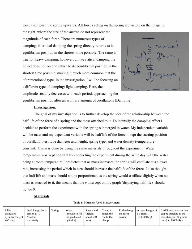
force) will push the spring upwards. All forces acting on the spring are visible on the image to

the right, where the size of the arrows do not represent the

magnitude of each force. There are numerous types of

damping, in critical damping the spring directly returns to its

equilibrium position in the shortest time possible. The same is

true for heavy damping, however, unlike critical damping the

object does not need to return to its equilibrium position in the

shortest time possible, making it much more common that the

aforementioned type. In the investigation, I will be focusing on

a different type of damping: light damping. Here, the

amplitude steadily decreases with each period, approaching the

equilibrium position after an arbitrary amount of oscillations (Damping).

Investigation:

The goal of my investigation is to further develop the idea of the relationship between the

half life of the force of a spring and the mass attached to it. To intensify the damping effect I

decided to perform the experiment with the spring submerged in water. My independent variable

will be mass and my dependant variable will be half life of the force. I kept the starting position

of oscillation,test tube diameter and height, spring type, and water density (temperature)

constant. This was done by using the same materials throughout the experiment. Water

temperature was kept constant by conducting the experiment during the same day with the water

being at room temperature.I predicted that as mass increases the spring will oscillate at a slower

rate, increasing the period which in turn should increase the half life of the force. I also thought

that half life and mass should not be proportional, as the spring would oscillate slightly when no

mass is attached to it, this means that the y intercept on my graph (displaying half life) should

not be 0.

Materials Table 1: Materials Used in experiment

1 liter graduated cylinder (height 465 mm)

Dual Range Force sensor at 10 Newton sensitivity

Spring Water (enough to fill the graduated cylinder)

Ring stand (height: about 500 mm)

Clamp to attach the rod to the clamp

Rod to hang the force sensor

A mass hanger of 50 grams ± .0001kg)( 0

6 additional masses that can be attached to the mass hanger (20 grams each) ± .0001kg)( 0

± .001N)( 0

Procedure

1. Fill a one liter graduated cylinder with water

2. Take the ring stand and attach the clamp to it at a height at which it will be a few

centimeters above the graduated cylinder

3. Attach the metal rod on the clamp (see figure 2)

4. Place vernier force meter (at 10 Newton sensitivity) on metal rod

5. Attach the spring on the force meter (see figure 2)

6. Attach the mass of 50 grams at the bottom of the spring

7. Place the graduated cylinder under the force meter in a manner that the spring

will be hanging at the center of the graduated cylinder

8. Adjust the height of the clamp so that the spring is submerged in the water

9. Compress the spring to its maximum

10. Measure force and time using logger­pro until ten oscillations are completed

11. Repeat 5 times

12. Place an additional mass of 20 grams on the mass hanger to change the

independent variable (see figure 1)

13. Repeat the process 5 times for each of the six remaining masses

Safety considerations

Even though this experiment is safe, one should make sure that the cylinder used tor the

experiment is deep enough. As the mass on the spring increases so will the amplitude of the

oscillations, hence if the amplitude is greater than the container depth the weights on the spring

will hit the bottom of the container, which could damage it. Additionally, the experiment should

not be performed close to electrical outlets. I performed the experiment on the floor instead of on

a desk to ensure that if the water spilled the computers would not get damaged.

Calculating half life:

My raw data only gives me force and time, meaning that I will have to calculate half life

using the below information.

From the physics curriculum we know that:

e F 10 = F o −λt

Where in my calculations will be the maximum force at the tenth oscillation. is theF 10 F o

maximum force of the first oscillation, t is the time it took for the spring to undergo ten

oscillation and is the decay constant which equals:λ

= λ t1/2ln(2)

Here is the half life. As a result through substitution we can solve for half life andt1/2

obtain:

Equation (2) t1/2 =tln(2)ln( )Fo

F 10

Raw data:

The force meter allowed me to measure

the change of force with time. A sample of

the first trail at 0.05 kilograms is visible at

the right. The data labeled in this picture

(maximum forces at the first and tenth

oscillation, and the time difference) can

be found in the three data tables below

with the averages of the five trials and

their

uncertainties.

Table 2: Maximum Force of Spring (as measured by force meter)at First Oscillation due to Mass

Mass (kg) Mass uncertainty (g) ± k

Average force at first oscillation (F)

Uncertainty of average force at first oscillation (1

) ±N

Average force at tenth oscillation (F)

Uncertainty of average force at tenth oscillation ( ) ±N

Average change in time between first and tenth oscillation (s) 2

Uncertainty Average change in time ( ) ± s

0.0500 0.0001 1.00 0.03 0.62 0.02 4.00 0.04

1 I used a dual range force sensor for Vernier to measure force and was in the range resolution of 0.01 however no uncertainties were given by the producer for this range, meaning that the uncertainty given is my estimation (I used the smallest significant figure the device could measure) 2 I used logger pro to measure time, no uncertainties for time were given by the program, hence I used the smallest significant figure the program displayed

0.0700 0.0002 1.27 0.02 0.802 0.007 4.59 0.01

0.0900 0.0003 1.59 0.04 0.97 0.04 5.02 0.02

0.1100 0.0004 1.87 0.03 1.16 0.004 5.52 0.02

0.1300 0.0005 2.12 0.04 1.33 0.01 5.97 0.05

0.1500 0.0006 2.33 0.04 1.506 0.005 6.38 0.08

0.1700 0.0007 2.65 0.08 1.64 0.01 6.76 0.02

Processed data:

After recording the raw data, I found half life using Equation (2), the different steps taken in

manipulating my raw data before being able to calculate half life are displayed below. The table

shows the result of dividing the maximum force measured by the spring at the first oscillation by

that at the tenth with the corresponding uncertainty for each mass. Next I took the natural

logarithm of this value, which can also be seen in the data table with the corresponding

uncertainties. Lastly, I found half life by dividing the time taken for the tenth oscillation to be

reached by the natural logarithm and multiplying this by the natural logarithm of two.

Table 3:Processed Data: Calculating Half Life

Mass (kg) Mass uncertainty (g) ± k

FoF 10

3 Uncertainty () ±

ln( )FoF 10

Uncertainty () ±

Half life (s) Uncertainty () ± s

0.0500 0.0001 1.6 0.1 0.47 0.06 5.9 0.8

0.0700 0.0002 1.59 0.04 0.46 0.02 6.9 0.4

0.0900 0.0003 1.6 0.1 0.50 0.07 7 1

0.1100 0.0004 1.61 0.03 0.48 0.02 8.0 0.4

0.1300 0.0005 1.60 0.04 0.47 0.03 8.8 0.6

0.1500 0.0006 1.55 0.03 0.44 0.02 10.1 0.6

0.1700 0.0007 1.61 0.06 0.48 0.04 9.8 0.8

Sample Calculation of half life:

3 The maximum force measured by the newton meter at the first oscillation divided by that at the tenth oscillation does not have units as these cancel through division

I will now more thoroughly show how I obtained half life and the uncertainty for half life at 0.05

kilograms.

Finding half life:

Equation (2) states that:

t1/2 =tln(2)ln( )Fo

F 10

At 0.05 kilograms the force meter measured an average of 1 Newton ( 0.03), at the tenth ±

oscillation this value dropped to an average of 0.62 Newtons ( 0.02), this change took 4 ( 0.04) ± ±

seconds. If we put all of these values into Equation (2) we obtain:

.9 s t1/2 =tln(2)ln( )Fo

F 10= ln( )1

0.62

4×ln(2) = 5

Uncertainty of half life:

To calculate uncertainty percent uncertainty of the three values must be found:

=ercent uncertainty of time P 00% 00% ± % TimeUncertainty × 1 = 4

±0.04 × 1 = 1

ercent uncertainty of force at first oscillation 00% 00% P = valueUncertainty × 1 = 1

0.03 × 1

± % = 3

ercent uncertainty of force at first oscillation 00% 00% P = valueUncertainty × 1 = 0.62

0.02 × 1

± .226% = 3

Next I found the uncertainty when the two forces are divided, by adding the two uncertainties: ncertainty of division of the forces .226 ± .226% U = 3 + 3 = 6

The value uncertainty of a natural logarithm is equal to the percent uncertainty of what

the logarithm is taken of divided by 100 (Propagation of Logarithms). This means that the

uncertainty of the logarithm of the division of both forces equals or 12.766%..06 ± 0 ±

Finally the uncertainty of half life will equal to the sum of the percent uncertainty of the

natural logarithm of the division of the forces plus the percent uncertainty of the time:

ncertainty half life % 12.766% ± 3.766% U = 1 + = 1 = .8s ± 0

Relationship between half life and mass

Were I to graph half life versus mass the concrete relationship (whether the line of best fit

is linear or not) would be unclear, as a result I had to find the accepted relationship using

formulas. Equation (2) states:

π T = 2 √ km

Additionally half life can be represented in terms of n periods:

T t1/2 = n

Here n does not need to equal an integer as the half life of the spring is a theoretical value. In

other words, there does not need to be a peak at half of the original force, rather half life can be

found in between two peaks. If we multiply equation (2) by n we get:

2π t1/2 = n √ km

t1/2 = √k2π√m × n2

Let m × n2 = u

Equation (3) t1/2 = √k2π√u

As n is not constant independently of mass, I calculated n at each mass.To find how many

periods there are in half life, half life simply needs to be divided by the period. Period will be

constant when mass is constant, hence it can be found by dividing the time for ten oscillations to

be completed by ten.

n = Period half life = t10

10 t1/2

After finding n, the product of m and n squared (u) was found as n changes with mass.

Multiplying the two will reduce my variables to two instead of three.

Table 4: Amount of periods (n) in each half life at each mass and mass times n squared

Mass (kg) Uncertainty ( kg) ±

Period (s) Uncertainty (s) ±

n Uncertainty ( ) ± u (kg) Uncertainty ( )g ± k

0.0500 0.0001 0.400 0.004 14 2 10 3

0.0700 0.0002 0.459 0.001 15.0 0.9 16 2

0.0900 0.0003 0.502 0.002 14 1 18 3

0.1100 0.0004 0.552 0.002 14.5 0.6 23 2

0.1300 0.0005 0.597 0.005 14.7 0.6 28 3

0.1500 0.0006 0.638 0.006 16 2 37 8

0.1700 0.0007 0.676 0.002 14.5 0.9 36 5

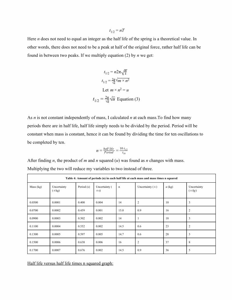
Half life versus half life times n squared graph:

Equation (3) predicts that the

relationship between the half life

and u should be a function to the

power of 0.5. This is approximately

the case in the above equation

which is to the power of 0.435.

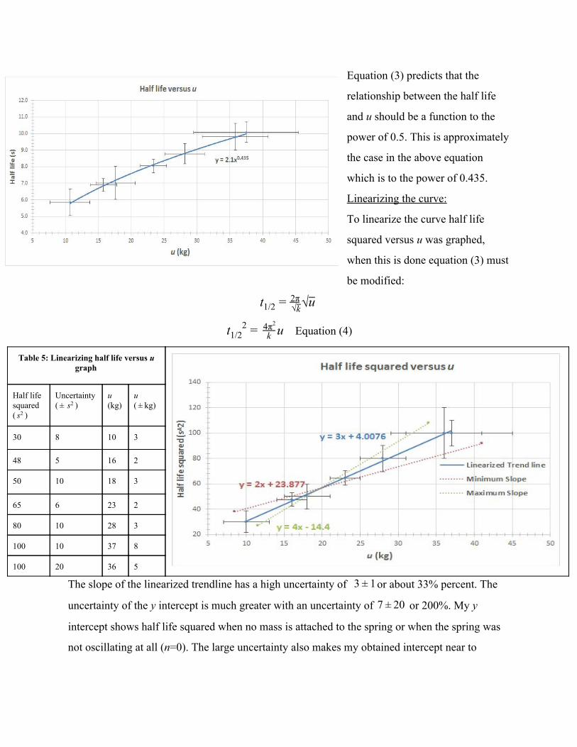
Linearizing the curve:

To linearize the curve half life

squared versus u was graphed,

when this is done equation (3) must

be modified:

t1/2 = √k2π√u

Equation (4)u t1/22 = k

4π2

Table 5: Linearizing half life versus u graph

Half life squared ( ) s2

Uncertainty ( )± s2

u (kg)

u ( kg)±

30 8 10 3

48 5 16 2

50 10 18 3

65 6 23 2

80 10 28 3

100 10 37 8

100 20 36 5

The slope of the linearized trendline has a high uncertainty of or about 33% percent. The 3 ± 1

uncertainty of the y intercept is much greater with an uncertainty of or 200%. My y0 7 ± 2

intercept shows half life squared when no mass is attached to the spring or when the spring was

not oscillating at all (n=0). The large uncertainty also makes my obtained intercept near to

insignificant, for instance a negative half life is impossible in this scenario yet it is supported by

my uncertainty. While this is due to limitations in my data collection, which will be discussed

later, it is also due to the large amount of data processing that was done to obtain this result.

Squaring n for instance doubled the variables percent uncertainty, so did squaring half life. When

half life was squared equation (4) was obtained:

u t1/22 = k

4π2

The equation clearly shows that is the slope of the trendline. As I was curious to see howk4π2

accurate my investigation was in terms of my slope (if there were great systematic errors

influencing my slope), I decided to find the spring constant using this slope and to compare it to

the actual value of the spring constant.

Finding spring constant using the slope

k4π2 = 3

3.159 N/m 3% 3N/m k = 34π2 = 1 ± 3 = 1 ± 4

Finding the actual spring constant

As k of the spring was not specified, I had to conduct a separate investigation to obtain

the constant by attaching separate masses to the spring and measuring the length of the spring.

The spring constant can be found by graphing force in Newton versus length of spring in meters.

The force is the weight of the masses (mass times 9.81). The data obtained from the experiment

is as follows:

Table 6: Alternate method of finding spring constant Weight (N)

Uncertainty Weight (

)±N

Length of Spring (m)

Uncertainty spring length ( )±N

0.491 0.001 0.1250 0.0005

0.687 0.002 0.1380 0.0005

0.883 0.003 0.1524 0.0005

1.079 0.004 0.1659 0.0005

1.275 0.005 0.1799 0.0005

1.472 0.006 0.1923 0.0005

1.668 0.007 0.2065 0.0005

No uncertainties for the slope were calculated as the uncerties were barely visible on the

graph, making them negligible. The slope of the graph,0.069m/N, is the reciprocal of the spring

constant, making the spring constant 14.49 N/m. I will assume this to be the actual value of the

spring constant in my comparisons.

Even though the uncertainty for the spring constant calculated using my slope was very

large, I was amazed to see how close the two values, 14.49 and 13 Newtons per meter,were to

each other, the spring constant found using the damping was about 10 percent too low. This is

well within my uncertainties.

Analysis and Evaluation:

My data shows that as the mass attached to the spring increases so does half life,

additionally the spring constant found, 13 Newtons per meter was ten percent too low. The ± 4

half life should almost be proportional to mass as the spring can still oscillate with no mass is

attached to it. This means that my y intercept in my linearized graph should be close to 0

however, when taking my uncertainty for the y intercept of 7 into account this cannot be0 ± 2

supported.

The largest contributor to my uncertainty and error bars in my graphs was half life. These

large uncertainties originate from my data’s large variation from each other at each mass, which

caused random error. This error could have originated from my procedure as I lifted, compressed

and let the spring into the water to start oscillating. While this occurred the spring did not always

fall perfectly straight into the water. In one trial the spring even grazed the glass of the test tube,

when this occurred the period, and force of the oscillations changed immensely. Even though, I

redid said trail the random error continuously occurred at a smaller magnitude and still exists in

my results. To reduce this random error I could use a wider test tube (if the spring passes close

the glass more turbulence will be created by the water particles reflecting of the glass).

Additionally the spring could be lifted out of and dropped into the water using a pulley. To do so

a string would have to be passed through the spring and tied to the mass, the other end of the

string would be put over a rod (or pulley) so that the string is perpendicular to the the water, if

the string is than pulled downward (over the rod) the spring will move upwards. If the string is

released the spring will move into the water,

perpendicularly and will start oscillating, a model of this

is displayed on the right.

Another source of error is that as masses were

added to the bottom of the spring, the volume of the

masses attached to the spring increased. If the

experiment were to be conducted in air, the buoyancy

force could be considered to be negligible, however in

water this is not the case as this force is much greater and

a doubling in volume will double this upward force. The force meter measured the “positive”

maximum force when the spring reached its maximum length, where the buoyant force opposed

the force of the spring. This means that the buoyant force reduced my results. To fix this error, I

could use masses that are more dense but have the same volume. In other words instead of

stacking the masses on top of each other I would use a single mass.

Conclusion:

The aim of my experiment was to find the relationship between the mass attached to a

damping spring and the half life of the force of the spring measured by the force meter. The

relationship I found was that as the mass attached on the spring increases, half life increases by

its square root. This supports my initial notion that half life would increase with mass. The two

variables should not be proportional to each other, however my results cannot fully support this

due to my large uncertainties. Additionally, as equation (3) had three variables, mass, n, and half

life it would be interesting to conduct an additional experiment to see how n changes with mass.

To do so the same experiment could be repeated but n would be graphed on the y axis and half

life divided by the square root of mass would be on the x axis .

Bibliography:

"Damping." Mini Physics. Mini Physics, n.d. Web. 06 Mar. 2016. <https://www.miniphysics.com/damping.html>.

"Propagation of Logarithms." Appendix A: Errors and Uncertainties. N.p., n.d. Web. 20 Mar.

2016. <http://phys114115lab.capuphysics.ca/App%20A%20­%20uncertainties/appA%20propLogs.htm>

"Simple Harmonic Motion." Wolfram Demonstrations Project (n.d.): n. pag. Web. 7 Mar. 2016.

<http://www.augusta.k12.va.us/cms/lib01/VA01000173/Centricity/Domain/396/Simple_Harmonic_Motion_(SHM).pdf>

Appendix

Raw data: The following are the raw data tables from my data collections with the

maximum force of the spring and the firsts and tenth oscillation and the time between the two

maximums recorded respectively.

Table 7: Maximum Force of Spring (as measured by force meter)at First Oscillation due to Mass

Trials showing the force measured by the force meter at the first oscillation (N) ( ).001± 0

Mass (kg)

Mass uncertainty (g)± k

1 2 3 4 5 Average Force (N)

0.0500 0.0001 1.016 1.028 0.954 1.004 0.991 1.00

0.0700 0.0002 1.249 1.274 1.268 1.286 1.286 1.27

0.0900 0.0003 1.556 1.575 1.605 1.624 1.593 1.59

0.1100 0.0004 1.845 1.876 1.900 1.869 1.845 1.87

0.1300 0.0005 2.115 2.102 2.164 2.096 2.139 2.12

0.1500 0.0006 2.373 2.237 2.348 2.373 2.342 2.33

0.1700 0.0007 2.673 2.643 2.569 2.68 2.68 2.65

Table 8: Maximum Force of Spring (as measured by force meter) at Tenth Oscillation due to Mass

Trials of force measured at maximum of the tenth oscillation by newton meter (N) ( ).001± 0

Mass (kg) Mass uncertainty (g)± k

1 2 3 4 5 Average Force (N)

0.0500 0.0001 0.604 0.629 0.623 0.617 0.636 0.62

0.0700 0.0002 0.807 0.807 0.801 0.801 0.795 0.802

0.0900 0.0003 0.985 0.979 0.979 0.925 0.979 0.97

0.1100 0.0004 1.163 1.157 1.163 1.163 1.157 1.16

0.1300 0.0005 1.311 1.323 1.335 1.329 1.329 1.33

0.1500 0.0006 1.501 1.507 1.507 1.507 1.507 1.506

0.1700 0.0007 1.642 1.642 1.642 1.636 1.654 1.64

Table 4: Change in Time from the First Maximum to the Tenth Maximum being reached for each Mass

Change in time for five trials(s) ( 0.02)±

Mass (kg)

Mass uncertainty (g)± k

1 2 3 4 5 Average Time (s)

0.0500 0.0001 4.00 4.00 4.04 3.98 4.00 4.00

0.0700 0.0002 4.60 4.60 4.58 4.58 4.59 4.59

0.0900 0.0003 5.02 5.00 5.02 5.02 5.02 5.02

0.1100 0.0004 5.52 5.50 5.52 5.52 5.52 5.52

0.1300 0.0005 5.94 5.92 6.00 5.96 6.02 5.97

0.1500 0.0006 6.38 6.40 6.40 6.40 6.32 6.38

0.1700 0.0007 6.78 6.76 6.76 6.74 6.78 6.76