Identifying Exercise of Market Power in CA Harvey-Hogan 12… · IDENTIFYING THE EXERCISE OF MARKET...

IDENTIFYING THE EXERCISE OFMARKET POWER IN CALIFORNIA

Scott M. Harvey* and William W. Hogan**

*LECG, LLC.Cambridge, MA

**Center for Business and GovernmentJohn F. Kennedy School of Government

Harvard UniversityCambridge, MA

December 28, 2001

i

Table of Contents

Page

EXECUTIVE SUMMARY iii

I. Introduction 1

II. Start-Up and Minimum Load Costs 3

A. What Is the Question? ...................................................................................................... 3

B. Is Alamitos 2 on June 17 Unique? ................................................................................... 6

C. Was Operation Profitable at Real-World Prices? .......................................................... 11

D. Would More Operation Have Been Profitable?............................................................. 17

E. Would Operation Have Been Profitable at Simulated Prices?....................................... 23

F. Does Market Design Matter? ......................................................................................... 261. Three-Part Bids ........................................................................................................ 272. Market Separation.................................................................................................... 283. Sequential Ancillary Service Markets ..................................................................... 284. Congestion Management ......................................................................................... 295. Bid Production Cost Guarantee ............................................................................... 306. Materiality of Market Design................................................................................... 30

G. Summary on Alamitos 2 and Similar Examples ............................................................ 33

III. Revised Price Simulation Analyses 33

A. Start-Up and Minimum-Load Costs............................................................................... 33

B. Environmental Restrictions............................................................................................ 35

C. Reserves ......................................................................................................................... 36

D. Outages .......................................................................................................................... 40

E. Other Features of the Model .......................................................................................... 411. Load Shape............................................................................................................... 412. Hydro and Geothermal............................................................................................. 413. Dispatch Instructions ............................................................................................... 424. Transmission Congestion......................................................................................... 435. Imports ..................................................................................................................... 43

F. Simulations .................................................................................................................... 45

IV. Withholding Analysis 47

A. Introduction.................................................................................................................... 47

B. Daylight Savings Time .................................................................................................. 48

C. Output Gaps on High-Priced Days ................................................................................ 54

ii

D. Output Gaps in High-Priced Hours................................................................................ 65

V. Physical Withholding 73

VI. Market Power Analysis 78

VII. Conclusion 80

iii


Scott M. Harvey and William W. Hogan

EXECUTIVE SUMMARY

The unexpected and suddenly high prices in the California electricity market, beginning in June2000, precipitated a variety of responses with far-reaching consequences. One central issuerequires identifying and analyzing the scope and significance of any exercise of market power.A complete analysis of this issue would be important, but has not been done. The nature of theCalifornia market and the highly stressed conditions of that period present significantcomplications in separating the exercise of market power from other activities that would havesubstantially different policy implications.

A full analysis of the exercise of market power would require use of data available to theCalifornia system operator but not available in the public domain. These data have not beendisclosed, nor apparently used in any study of the California market. However, the importance ofthe matter has prompted use of the publicly available data to attempt to assess the relativeimportance of market power in the California crisis. Employing simulation models to estimateprices and other approaches to identify economic and physical withholding, a series of studieshave been offered in support of a conclusion that there was substantial market power exercised inCalifornia.

By contrast, another series of sensitivity analyses have concluded that the simplifyingassumptions of the simulation models and the other analyses with publicly available data wereenough to introduce errors as large as the effect that was to be estimated. In other words, thepublicly available data were not up to the task of detecting a substantial exercise of marketpower.

The present paper stands in this series of analyses with conflicting conclusions. Here we gofurther into the sensitivity analyses in response to previous comments and critiques. Theprincipal purpose is to clarify and bolster the analysis of what is at issue and why the impacts ofthe simplifications are not on their face either negligible or irrelevant.

Our further sensitivity analyses reinforce the conclusion that we cannot demonstrate theexistence or the absence of an exercise of market power. However, there is no ambiguity in theconclusion that there are other features of the California market design that are fundamentallyflawed and need to be corrected as part of the unique situation in California and the largerdiscussion of the implementation of Regional Transmission Organizations. These market reformswould be important no matter what the resolution of the analysis of the exercise of marketpower.

1


Scott M. Harvey and William W. Hogan1

December 28, 2001

I. INTRODUCTION

The tumult of the California electricity market and high prices beginning in June of 2000 raisedthe specter of an exercise of market power. A complete analysis of this issue would be important,but has not been done. Given the importance of the issues, however, even incomplete data havebeen applied and spawned debates about the size and scope of the exercise of market power. Arecent paper of ours discusses further some of the theoretical issues and explains why weconclude that this is an empirical question.2 Ideally, we would wait until all the data wereavailable to address the empirical matters, but the importance of the issue and the pace of eventspreclude this more deliberate approach. Here we continue the discussion of the empiricalmatters, carrying further the sensitivity analyses and using some additional information obtainedfrom the Mirant Corporation, which sponsored this work. The conclusion remains that:

"With the available data in the public domain, and the special complicationsintroduced by the California market design, the margin of error in estimating theextent of the possible exercise of market power through strategic withholding ofelectric generation is of the same order of magnitude as the effect being measured.On balance, to date the publicly available data provides no reason for the FederalEnergy Regulatory Commission to change its conclusion that there is no evidenceof strategic withholding nor any proof that no strategic withholding has occurred.

1 Scott Harvey is a Director with LECG, LLC, an economic and management consulting company. William

Hogan is the Lucius N. Littauer Professor of Public Policy and Administration at the John F. Kennedy Schoolof Government, Harvard University. This paper was supported by Mirant. The authors are or have beenconsultants on electricity market design and transmission pricing, market power or generation valuation issuesfor American National Power; Brazil Power Exchange Administrator (ASMAE); British National GridCompany; Calpine Corporation; Commission Reguladora De Energia (CRE, Mexico); Commonwealth Edison;Conectiv; Constellation Power Source; Detroit Edison; Duquesne Light Company; Dynegy; Edison ElectricIntitute; Electricity Corporation of New Zealand; Electric Power Supply Association; Entergy; General ElectricCapital; GPU, Inc. (and the Supporting Companies of PJM); GPU PowerNet Pty Ltd.; ISO New England;Midwest ISO; National Independent Energy Producers; New England Power; New York Energy Association;New York ISO; New York Power Pool; New York Utilities Collaborative; Niagara Mohawk Corporation;Ontario IMO; PJM Office of the Interconnection; Pepco; Public Service Electric & Gas Company; ReliantEnergy; San Diego Gas & Electric; Sempra Energy; Mirant/Southern Energy; SPP; TransÉnergie; Transpowerof New Zealand Ltd.; Westbrook Power; Williams Energy Group; and Wisconsin Electric Power Company.John Jankowski, Christine Jimenez, Sherida Powell, Joel Sachar, Erik Voigt and Matthew Kunkle providedcomments and research assistance. The views presented here are not necessarily attributable to any of thosementioned, and any errors are solely the responsibility of the authors.

2 Scott M. Harvey and William W. Hogan, “Further Analysis of The Exercise Of Market Power In TheCalifornia Electricity Market,” November 21, 2001, hereafter Harvey-Hogan (November).

2

By contrast, there is general agreement that the California electricity marketdesign is 'seriously flawed.' Furthermore, there is evidence that the policyresponses that have been adopted in California have accelerated an alreadyserious market collapse. Hence, without dismissing the possibility of the exerciseof market power, the principal policy focus should be on fashioning workablesolutions for the other more serious problems in market design that relate to theunderlying causes of the market meltdown."3

The proximate motivation of the present paper is to continue the discussion extended in the July2001 Joskow and Kahn paper4 commenting on our April 2001 paper,5 which raises fourempirical issues affecting the analysis of the exercise of market power in California. First,Joskow-Kahn argues that if minimum load costs are taken into account, the units that actuallyoperated in California during high priced hours in June 2000 were not losing money.6 Asdiscussed further below, this is not the issue we raised. Rather, we asked whether the units thatdid not actually operate in California during high-priced hours in 2000 could have operatedprofitably at the simulated prices and further suggested that one cannot answer this questionwithout taking account of start-up and minimum load costs. Moreover, the data consistentlyshow that these costs are sufficiently large in magnitude to materially impact the answer to thisquestion.

Second, Joskow-Kahn states that after modifying the simulation model to take account of theissues we raised in our April paper, they still find that their simulated price of electricity inCalifornia is materially less than real-world prices during June 2000.7 They interpret this asevidence that could best be explained as an exercise of market power through withholding ofcapacity. The new simulation model, however, largely does not address the problems we pointedout in April and introduces new problems that predictably underestimate competitive prices.Simulation models that leave out important real supply constraints will predictably calculateprices that are lower than real-world prices, but such a difference does not provide a basis forconclusions regarding the existence or exercise of market power.

Third, Joskow-Kahn repeats the withholding analysis for somewhat different combinations ofhours than in their earlier paper and again find an output gap.8 The calculations largely ignorethe observations we made in our April paper and the limitations remain. That is, the output gapincludes the capacity of unavailable units, excludes deratings or environmental outputlimitations, uses capacities that may overstate the sustainable output of the units, and ignoreswhether units were coming on-line or would have been changing their output in response to

3 Harvey-Hogan (April), p. ii.4 Paul Joskow and Edward Kahn, "Identifying the Exercise of Market Power: Refining the Estimates," July 5,

2001 (hereafter referred to as Joskow-Kahn (July)).5 Scott M. Harvey and William W. Hogan, “On the Exercise of Market Power Through Strategic Withholding in

California,” April 24, 2001 (hereafter Harvey-Hogan (April)).6 Joskow-Kahn (July), pp. 5, 14-17.7 Joskow-Kahn (July), p. 13.8 Joskow-Kahn (July), pp. 19-20, 27.

3

sudden price changes. The magnitude by which these calculations overstate the actual outputgap can be seen by analyzing the output gap calculated using the methodology during the hoursof stage 1 and stage 2 emergency in which it is known that there was a shortage of capacity atany price.

Fourth, they state that they find clear evidence of physical withholding,9 but Joskow-Kahnprovides no supporting evidence.

II. START-UP AND MINIMUM LOAD COSTS

A. What Is the Question?

The example of Alamitos 2 on June 17, 2000 was used in Harvey-Hogan (April) to make ananalytical point. In particular, neglect of start-up, minimum load costs and operating limitationscould result in material errors in an estimation of profitability, especially important for marginalunits. The choice of Alamitos 2 was made because of its characteristics and because on June 17we had real data for operations over a wide range of plant output conditions. The data showedthat ignoring these complicating factors would result in material errors in calculating theprofitability of this marginal unit, to the extent of the possibility that it lost money fromoperating.

Joskow-Kahn argues that the particular results for Alamitos 2 were rare or unique. Joskow-Kahn’s discussion of the Alamitos 2 example misses the point of the example and our paper, anddoes not address the discussion of an important limitation of the simulation analysis. Joskow-Kahn suggests that we have argued that our calculations of the profitability of Alamitos 2 onJune 17, 2000 demonstrate that other units actually operating on high priced days during June2000 operated unprofitably.10 This was not what we said and not the point of the example.Indeed, such a claim would be irrelevant to the issues we have raised. We discussed theAlamitos 2 example in the context of the Joskow-Kahn simulation analysis.11 Our point was andis that because the simulation methodology does not take account of start-up costs, minimumload costs, and unit inflexibilities such as minimum down times and up times, the simulationmethodology does not replicate the choices that would determine the competitive level ofelectricity prices.

Tables 7, 8, and 9 in our April paper focused on the material difference between the apparentprofitability of operating Alamitos 2 in an economic evaluation based on incremental heat ratesand units that can turn on and off, hour to hour, and the real-world profitability of Alamitos 2.The difference was large. The point of this example was and is that simulations that dispatchgeneration to meet load and estimate prices based on incremental heat rates, in non-chronologicalmodels that do not consider start-up and minimum load costs or unit inflexibilities, will meet

9 Joskow-Kahn (July), p. 23.10 Joskow-Kahn (July), pp. 14.11 Harvey-Hogan (April), pp. 25-33.

4

load with resources that could not always have operated profitably at those prices in the realsystem. As a result, the simulated prices may not measure the competitive level of energy prices.

Given the complexity of the market, it is not surprising to find an example of a plant actuallyoperating and losing money even though prices were high in some hours. However, the Joskow-Kahn withholding conclusion does not depend only on showing that this event is rare or unique.The Joskow-Kahn conclusion requires showing that at even lower prices, the errors in calculatingprofitability would be negligible and that plants that were not operating would have beenprofitable. Furthermore, given the evidence of Alamitos 2 of the magnitude of the differencebetween profitability evaluated hour by hour based on incremental energy costs and profitability,when evaluated taking account of actual heat rates and the constraints of minimum load andstart-up costs, it would be surprising to find that all of the plants that were not operating in thereal-system but were dispatched based on incremental energy costs in the simulation couldactually have operated profitably at much lower prices if we account for all of the costs.

It is not responsive to this observation and example to state that other units actually operating onJune 17, or even all other units actually operating on every other high priced day, were profitableto operate based on real-world output, real world prices and actual operating patterns. The issueis whether the resources that were not used to meet load in the real world but were used to meetload in the simulation could actually have operated profitably at the simulated prices.

In using Alamitos 2 as an illustration of the importance of actual generator cost functions andinflexibilities, we had in mind a set of 13 generators included in the Joskow-Kahn simulationstudy that have relatively high heat rates for the minimum load block, as portrayed in Table 1. Itcan be seen based on the Klein and CEMS data reported in Table 1 that all of these units haverelatively high minimum-load heat rates and some also have relatively high emissions rates. Sixof these units, Alamitos 1 and 2, El Segundo 1 and 2 and Redondo Beach 5 and 6 (the “SicklySix?”) also have relatively high NOx emissions rates. In aggregate, these 13 units account forroughly 2,929 MW of capacity, so whether they are on line and operating would have a materialimpact on supply and prices.

5

Table 1Characteristics of High Cost Units

Full Load

MinimumLoad

Heat Rate(A)

EmissionsRate(B)

IncrementalHeat Rate

(C)

AverageHeat Rate

(D)

MinimumLoad Block

(E)

KleinCapacity

(F)

Alamitos 1 28,899 0.123 10,056 10,663 10 175

Alamitos 2 28,899 0.189 10,056 10,663 10 175

Alamitos 3 25,283 0.076 9,338 9,898 20 320

Alamitos 4 25,283 0.060 9,338 9,898 20 320

El Segundo 1 27,838 0.125 9,901 10,591 10 175

El Segundo 2 27,838 0.136 9,901 10,591 10 175

El Segundo 3 24,628 0.061 9,201 9,741 20 335

Etiwanda 1 24,848 0.081 10,724 11,072 10 132

Etiwanda 2 24,848 0.089 10,724 11,072 10 132

Etiwanda 3 22,980 0.047 9,292 9,731 20 320

Etiwanda 4 22,980 0.049 9,292 9,731 20 320

Redondo Beach 5 31,617 0.168 9,532 10,530 10 175

Redondo Beach 6 31,617 0.094 9,532 10,530 10 175

Sources:Cols. A, C, D, E, F – Joel Klein, “The Use of Heat Rates in Production Cost Modeling and Market Modeling,”April 17, 1998 (hereafter Klein (April 1998)).Col. B emissions 2Q, 2000 CEMS.

Asking whether there were many units that were actually operating in the real world on highpriced days that would have lost money at actual PX day-ahead prices has little bearing on theissue we raised. One question that would be relevant would be to ask whether any of the unitsthat were not operating in the real world, but were dispatched to operate in particular hours in theJoskow-Kahn simulation, would have been profitable or unprofitable to operate in those hours atreal-world prices taking into account real-world minimum load costs and operating inflexi-bilities. A second question to ask would be whether the units that actually were operating in thereal world, would have been able to operate profitably at the prices simulated by Joskow andKahn. Joskow and Kahn did not address either question in their reply. Instead, they suggest thatthe units that actually operated in the real world, operated profitably in the real world, evaluatedat real-world prices. Whether this claim is correct or not, it is largely irrelevant to the issues wehave raised regarding their simulation methodology.

6

B. Is Alamitos 2 on June 17 Unique?

In discussing our example of Alamitos 2 on June 17, Joskow-Kahn suggests that our statementthat our “calculations for Alamitos 2 are only illustrative and we have not repeated this calcula-tion for every unit for every day of June. The point of these calculations is that the financialimpact of minimum load costs and operating inflexibilities is not necessarily insignificant”12 wasmisleading. They suggest that this statement was misleading because:

“readers may gain the impression that the Alamitos 2 example is typical of otherunits on other days and that “unprofitability” is an important explanation for thewithholding behavior that we identified. However, Harvey & Hogan do notactually display similar calculations for any other units or days. We have nowperformed profitability calculations for every day listed in Table 5: the dayswhich have the high-price hours that we focus on in our analysis of withholdingbehavior. This task was not unduly onerous, and Harvey-Hogan could haveperformed it had they wished. We find that there was only one unit on one day inJune which was unprofitable under the Harvey-Hogan criteria using hourly CEMSdata to account for minimum-load costs.”13

The Joskow-Kahn comments are misdirected on several matters. First, the point of our analysiswas not that the units that actually operated on high priced days in the real world were operatingunprofitably in the real world. Our point was that ignoring minimum load costs and physicalunit characteristics materially changes the apparent profitability of supplying output, andanalyses that ignore these costs are estimating a supply curve that may be materially differentfrom the real supply curve. Not only did our quoted statement explicitly refer to the financialimpact of minimum load costs and operating inflexibilities, but it followed six pages discussinghow the apparent profitability of supplying incremental output changed when minimum loadcosts and inflexibilities were taken into account.14 It is even more surprising to miss the point ofour comment since it appeared directly below Table 9 in the April paper, reproduced as Table 2below with one adjustment.

The Alamitos 2 example shows the potential for mistaken conclusions regarding the profitabilityof increased output that arises when these added costs are ignored. The problem would becompounded if in place of the actual prices observed in the market the profitability analysis weredone at the lower prices in the Joskow-Kahn simulation.

Table 9 in our first paper used the same set of “profitable hours” whether allowance costs wereadded or not. The calculations in Table 2 only include as profitable those hours that wereprofitable with allowance costs included. Tables 3 through 6 follow this convention. Table 9does not merely report that the operation of Alamitos 2 would have been unprofitable undercertain assumptions. Instead, it portrays a series of comparisons illustrating how substantially theapparent profitability of operation could change, when account was taken of minimum load costs

12 Harvey-Hogan (April), p. 32.13 Joskow-Kahn (July), p. 15.14 Harvey-Hogan (April), pp. 25-32.

7

and operating inflexibilities. This difference is important in assessing whether units that were notoperating in the real world could have operated profitably in the real world in the hours theJoskow-Kahn simulation dispatches them based on their incremental costs. Moreover, thisdifference is also important in assessing whether units that did operate in the real world couldhave operated profitably at the prices simulated by Joskow and Kahn, rather than at real-worldprices. Joskow-Kahn addresses neither of these issues in the reply.

Table 2Alamitos 2 Profitability June 17, 2000

With and Without Emissions Allowance CostsAll Hours Profitable Hours

No AllowanceCosts

AllowanceCosts

No AllowanceCosts

AllowanceCosts

Actual Heat Rate (1,724) (36,382) 22,119 7,981

Incremental Heat Rate 45,573 25,027 47,870 30,906

Notes:Actual heat rate calculations use the SP-15 PX price.Incremental heat rate calculations use the unconstrained PX price.Gas Price = $4.99.Allowance Cost = $10/lb.Emissions Rate = 0.189 lb./mmBtu per CEMS.Calculated profitability does not include variable O&M or station costs.CEMS data are not adjusted for Daylight Savings Time.Source:Harvey-Hogan (April), Table 9, p. 32.

Instead, Joskow-Kahn addresses the implications of not calculating the profitability at real pricesof the units that were actually operating on 14 high priced days. Joskow and Kahn indicate thatthey have made a similar calculation for every unit on these 14 days (not every day in June) andhave found that Alamitos 2 is unique.15 In fact, however, they did not repeat our calculations toshow the change in apparent profitability when start-up costs, minimum-load costs and unitinflexibilities are taken into account for even a single unit on a single day, let alone for every uniton many days. The calculations in Table 9 of our April paper, reproduced as Table 2 above,calculated the apparent profitability of Alamitos 2 operation under a variety of assumptionsregarding heat rates, allowances and inflexibilities to show the large differences in apparentprofitability of operating Alamitos 2 in the real world and in the Joskow-Kahn simulation.16

15 Joskow-Kahn (July), p. 15.16 The calculations based on the actual heat rate also used the actual SP-15 day-ahead price, while the calculations

using the incremental heat rate used the hypothetical PX unconstrained price to which Joskow and Kahn(March) compared their simulation results (p. 14).

8

There is no such calculation in the Joskow-Kahn paper.17 To make the point, we do not needrepeat these calculations for every unit on every day. We have repeated them for Alamitos 3 and4 on June 17 and 23, days on which the calculations show that the operation of these units wouldhave been profitable at real-world PX prices (see Tables 3 to 6 below). Our comparisons againshow, however, that the apparent profitability of operating these units is materially affected if thecalculation does not take account of actual heat rates, minimum load costs and operatinginflexibilities. We have now undertaken these calculations for five unit days, which reinforcesthe point that the changes matter.

On June 17, the difference between the apparent profitability of operating Alamitos 3 and 4based on incremental heat rates for the profitable hours of the day was approximately $100,000higher than the profitability evaluated at actual heat rates over the day as a whole. This is an evenlarger error than in the case of Alamitos 2 on June 17.

The impact on prices could be important. For instance, a 200 MW plant operating with 5high-priced hours over the day would need a price increase of $1/MW to make up each $1,000 ofcost difference.18 Hence, a price increase of $100/MW would be required during these high-priced hours to make up a $100,000 difference in profits. How this would play out in thecomplex California market is far from certain, but the error does not appear on its face to benegligible.

17 The comparisons in the April paper would be slightly affected by adjusting the CEMS data for Daylight Savings

Time, discussed in Section IV below. The adjusted comparison is:

Table 2 (Adjusted CEMS Data)Alamitos 2 Profitability June 17, 2000


No AllowanceCosts

AllowanceCosts

No AllowanceCosts

AllowanceCosts

Actual Heat Rate (43) (34,585) 22,902 8,752Incremental Heat Rate 46,710 26,279 48,530 31,324Notes:Actual heat rate calculations use the SP-15 PX price.Incremental heat rate calculations use the unconstrained PX price.Gas Price = $4.99.Allowance Cost = $10/lb.Emissions Rate = 0.189 lb./mmBtu per CEMS.Calculated profitability does not include variable O&M or station costs.

18 The numbers are illustrative for simplicity. The Alamitos 2 plant has a Klein capacity of 175 MW.

9

Table 3Alamitos 3 Profitability June 17,2000


No AllowanceCosts

AllowanceCosts

No AllowanceCosts

AllowanceCosts

Actual Heat Rate 118,186 79,746 145,828 119,543


Notes:Actual heat rate calculations use the SP-15 PX price.Incremental heat rate calculations use the unconstrained PX price.Gas Price = $4.99.Allowance Cost = $10/lb.Emissions Rate = 0.076 lb./mmBtu per CEMS.Calculated profitability does not include variable O&M or station costs.CEMS data, adjusted for Daylight Savings Time.



No AllowanceCosts

AllowanceCosts

No AllowanceCosts

AllowanceCosts

Actual Heat Rate 114,489 83,242 143,262 122,033



On June 23, the difference between the profitability of operating evaluated based on incrementalheat rates in the profitable hours and based on actual heat rates over the day was lower, but stillexceeded $40,000 for both of these units.

10



No AllowanceCosts

AllowanceCosts

No AllowanceCosts

AllowanceCosts

Actual Heat Rate 328,036 286,047 343,258 309,615



Table 6Alamitos 4 Profitability June 23, 2000


No AllowanceCosts

AllowanceCosts

No AllowanceCosts

AllowanceCosts

Actual Heat Rate 320,302 287,111 337,129 310,529



Hence, the example of Alamitos 2 on June 17 was not unique, for the point it was offered toillustrate.

11

C. Was Operation Profitable at Real-World Prices?

Second, Joskow and Kahn’s comment is also mistaken in suggesting that the operation of all ofthese units would have been profitable at PX prices for their real-time output during theserelatively high priced days, taking into account minimum load costs and average heat rates. Inreality, the six high cost units (Alamitos 1, 2; El Segundo 1, 2; Redondo Beach 5 and 6) wereoperating on the days of June 17, 21 and 23 in only nine instances and their operation wouldhave been unprofitable at PX prices and actual output in six of these instances, when emissionallowance costs are taken into account (see Table 7 below, and Table 7 in Joskow-Kahn(July)).19

Table 7High Heat Rate Unit Operating Profitability

Day-Ahead PX Prices and Real-Time SchedulesJune 16, 2000 June 17, 2000 June 21, 2000 June 23, 2000

Alamitos 1 -- -- (13,144) (3,991)Alamitos 2 146,884 (34,585) (20,502) 15,615

Alamitos 3 1,427,307 79,746 65,164 286,047Alamitos 4 1,401,572 83,242 72,084 287,111

El Segundo 1 224,362 -- -- --

El Segundo 2 239,846 -- 19,904 (12,230)

El Segundo 3 113,506 27,937 -- 169,447Etiwanda 1 358,102 -- -- --

Etiwanda 2 301,613 -- -- --Etiwanda 3 1,021,846 66,865 (998) 260,470

Etiwanda 4 902,691 51,400 (315) 270,656Redondo Beach 5 -- -- -- --

Redondo Beach 6 -- -- (18,235) 4,921Notes:CEMS heat rates.Gas Price = $4.99.Allowance Cost = $10/lb.Emissions rates per CEMS.Price = SP-15 PX price.Calculated profitability does not include variable O&M or station costs.CEMS data, adjusted for Daylight Savings Time.

19 See Joskow-Kahn (July) Table 7, p. 17.

12

Joskow and Kahn reach the conclusion that the operation of several of these units would havebeen profitable in the real world by apparently either omitting emissions costs20 or adding toprofits their assessment of ancillary service revenues. Emission costs were included in our earlieranalysis and as seen in Table 7 (as well as Table 7 in the Joskow-Kahn reply), the operation ofseveral additional units was unprofitable applying the criteria used in our April paper.

The Joskow-Kahn conclusion that the operation of all of these units would have been profitableat real-world prices may be based on calculations that include additional revenues that Joskowand Kahn attribute to the supply of ancillary services,21 a revenue source not included in ouroriginal illustration.22 It could be appropriate to include estimated ancillary service costs in anassessment of the profitability of unit operation. Recall, however, that the point of our originalanalysis was to illustrate the impact of alternative assumptions regarding minimum load costsand operating inflexibilities on apparent profitability. If one were interested in the absoluteprofitability of these units, rather than the change in apparent profitability, it would be necessaryto take account of variable O&M costs (not included in the Joskow-Kahn profitabilitycalculations) and to calculate revenues based on the net output available for sale, rather thangross output including electricity consumed at the plant.23 Table 9 in our April paper noted thatwe were omitting both of these costs from our illustrative calculations, which as we haveobserved above, were intended to illustrate the error in profitability estimates if minimum loadcosts are nor taken into account. Moreover, the Joskow-Kahn estimates of ancillary servicerevenues have a number of problematic features.

The first limitation of the Joskow-Kahn assessment of ancillary service revenues is that thecalculations appear to assume that the same ramping capacity could be used to simultaneouslyprovide AGC, spinning reserve and non-spinning reserve.24 In reality, the ten-minute rampingcapability could be used only to provide ten minutes of ramping capability of spinning and non-

20 Joskow-Kahn (July), p. 15-16.21 Joskow-Kahn (July), p. 17.22 This was pointed out in our paper in observing that our calculations did not reflect the actual day-ahead

revenues. Harvey-Hogan (April), footnote 54, p. 28.23 This was noted in Harvey-Hogan (April) (footnote 52, p. 26 and the notes for Tables 6, 7, 8 and 9). The CEMS

data on which we, and Joskow and Kahn, have based these calculations measure the gross output of the units(which includes electricity consumed in operation of the units, i.e., station costs). Other factors not included inthese calculations are the actual level of day-ahead sales (day-ahead sales could have been either greater or lessthan real-time output) and actual incremental emissions (the average emissions data may not reflect actualemissions for these particular dispatch patterns). Moreover, Alamitos 4 and Redondo Beach 5 and 6 were RMRunits and may have opted to operate at contract rather than market rates because day-ahead prices were too lowto recover their costs.

24 We have not been able to locate the “publicly available” RMR contracts between the generators and the ISOs onwhich Joskow and Kahn state they relied in their ancillary service analysis. We have, however, obtained similardata for a number of the units from the divestiture disclosure documents. See “Capacity Sale and TollingAgreement by and among AES Alamitos, L.L.C., AES Huntington Beach, L.L.C., AES Redondo Beach,L.L.C., and Williams Energy Services Company,” Schedule A, FERC Docket No. ER98-2184, -2185 and –2186, July 15, 1999. See also “Application for Authority to Sell Specific Ancillary Services at Market-basedRates and Request for Expedited Consideration,” FERC Docket No. ER98-2977, May 13, 1998. The Etiwandaunits are not included in the discussion below because we have not been able to locate data on their ramp rates.

13

spinning reserves in total.25 This assumption serves to overstate ancillary service capacity andrevenues. Second, they prorate down the amount of ancillary services any individual unit couldhypothetically provide based on total ancillary services supplied. While this adjustment makestheir revenue figures look more reasonable, it has no economic basis. If these units couldeconomically supply the assumed amount of ancillary services, they could have bid all of it intothe market, not merely a prorated share of it. Thus, this procedure tends to understate potentialancillary revenues and offset the first methodological problem. Third, the ancillary service profitcalculations are based on the higher of day-ahead or real-time prices.26 This approachunambiguously overstates the profits that real-world firms could derive from the sale of ancillaryservices. Fourth, much of the assumed ancillary service revenues derive from the supply ofregulation, but no account is taken in these calculations of the increased operating costs in termsof higher heat rates that are associated with the provision of regulation. The provision ofregulation by these steam units would indeed be highly profitable at these prices if it werecostless, but it is not costless, which is why regulation prices are high.27 Fifth, although Joskowand Kahn state that they used RMR data on AGC minimum operating levels,28 the illustrativecalculations they provide assign regulation to several units that appear to have been operatingwell below their AGC minimums.29

To provide a better reflection of plausible ancillary service revenues, we have estimated ancillaryservices revenues for the units and days in Table 7 above assuming that each unit sold capacityequal to its 10 minute ramp rate (up to total unit capacity) at the day-ahead spinning reserveprice, or at the 50-50 weighted average of the day-ahead spinning reserve and non-spinningreserves prices. We have not added any allowance for AGC profits because the calculation ofsuch a profit margin requires knowledge of the cost of providing AGC (in terms of the heat rateperformance penalty) on these units. While the inclusion of estimated ancillary servicesrevenues makes operation profitable for one unit on June 23, the operation of several unitsremains unprofitable on June 17 and 21.

25 See Yenren Liu, Mark Rothleder, Ziad Alaywan, Mehdi Assadian, and Farrokh A. Rahimi, “Implementing

Rational Buyer’s Algorithm at California ISO,” August 17, 2001. Joskow and Kahn “account for how muchcapacity has already been scheduled for the generator,” p. 33, but the capacity limit appears to have been thetotal capacity of the unit, rather than the ten-minute ramping capacity.

26 This is not stated in the Joskow-Kahn Reply and Joskow and Kahn did not identify the prices used in thiscalculation, but it is apparent that revenues reported in Table A2.2 Joskow-Kahn (July), p. 34 were based onhour-ahead ancillary service prices for June 21 as hour-ahead spin and non-spin prices were high while day-ahead prices were quite low. The revenues reported for June 23, however, must have been calculated based onday-ahead prices as non-spin prices were quite low in the hour-ahead market.

27 Although the cost of regulating may at the margin be set by steam units, most of California’s regulation waslikely provided by hydro units which do not incur similar costs in providing regulation. The price of regulationwould therefore likely be set by the costs of the steam units that could most efficiently provide this service, andthe supply of regulation would likely have been uneconomic for run of the mill steam units.

28 Joskow-Kahn (July), p. 32.29 Joskow-Kahn (July), p. 33. For example, Table A2.1 shows that, according to the CEMS data, in the first hour

of June 21, 2000, Alamitos 1 generated 12 MW. Joskow and Kahn ascribe 105 MW of capacity available toprovide regulation up. However, according to the “Capacity Sale and Tolling Agreement,” the unit is not AGCcapable at this level of output, but needs to produce at 40 MW before it becomes AGC capable. Similarly,Huntington Beach 1 is shown with output of 21 MW, with 129 MW available for regulation up. According tothe “Capacity Sale and Tolling Agreement,” this unit is not AGC capable in the 20-65 MW range.

14

Table 8High Heat Rate Unit Operating Profitability with Spinning Reserve Revenues

PX Profits June 16, 2000 June 17, 2000 June 21, 2000 June 23, 2000

Alamitos 1 -- -- (6,066) 18,194Alamitos 2 273,330 (31,351) (13,526) 37,800Alamitos 3 1,456,940 80,771 71,347 290,344Alamitos 4 1,455,769 85,010 76,070 292,958El Segundo 1 350,681 -- -- --El Segundo 2 366,165 -- 25,197 (11,273)El Segundo 3 311,935 34,129 -- 211,916Redondo Beach 5 -- -- -- --Redondo Beach 6 -- -- (13,296) 27,106Notes:Ancillary services revenues are calculated for those hours in which the unit had positive generation.Etiwanda units are not included because we lack ramp rates for those units.CEMS data, adjusted for Daylight Savings Time.Energy revenues from Table 7.Calculations do not include variable O&M or station costs.Day-ahead ancillary service prices were used.

Table 9High Heat Rate Unit Operating Profitability with Ancillary Service Revenues

50% Spinning Reserve, 50% Non-Spinning Reserve


Alamitos 1 -- -- (6,712) 79,657Alamitos 2 247,884 (31,362) (14,141) 99,262Alamitos 3 1,447,841 81,013 70,737 296,573Alamitos 4 1,442,668 85,090 75,683 302,681El Segundo 1 325,264 -- -- --El Segundo 2 340,748 -- 24,806 (11,282)El Segundo 3 281,804 34,107 -- 329,572Redondo Beach 5 -- -- -- --Redondo Beach 6 -- -- (13,343) 88,568Notes:Ancillary services revenues are calculated for those hours in which the unit had positive generation.Etiwanda units are not included because we lack ramp rates for those units.CEMS data, adjusted for Daylight Savings Time.Energy revenues from Table 7.Calculations do not include variable O&M or station costs.Day-ahead ancillary service prices were used.

15

Moreover, it should be recognized that the profitability portrayed in Tables 8 and 9 is theprofitability of generation able to bid into day-ahead markets such as those coordinated by PJM-ISO and the NYISO, in which the generator submits three part bids and its schedule is optimizedover the day. California generators did not have the option of bidding into such a market. If suchan option existed, perhaps market performance would have been different.30

Joskow-Kahn also suggests that real-time revenues could increase the profitability of operationon days with high–real-time prices.31 This is correct on days on which real-time prices werehigher than day-ahead prices, but output that is not sold at day-ahead prices may also be sold atreal-time prices that are lower than day-ahead prices, as was the case on June 16, 17 and 23.

In fact, all but one of the nine high cost units we have discussed lost money by operating in real-time on June 16 and 17 (El Segundo 3 on June 16 under one measure of potential real-timeancillary service revenues). That is, with the benefit of perfect hindsight, they should have shut-down and covered their day-ahead positions (if any) at real-time spot prices.32 This is truewhether ancillary service revenues are calculated as 100 percent spinning prices or 50 percentspinning and 50 percent non-spinning prices and even though no account is taken of variableO&M costs or station costs (see Tables 10 and 11). Moreover, on June 23 the more efficient ofthese plants were profitable to operate at real-time prices, but every one of the high-cost six thatwas operating, was unprofitable to operate at real-time prices. Once again, with the benefit of20-20 hindsight, the plants should have been taken off line.

30 This point is discussed below in Section F.31 Joskow-Kahn (July), p. 17.32 Alamitos 4 and Redondo 6 are RMR units and may have had RMR schedules requiring their operation on some

or all of these days.

16


Actual Real-Time Energy and Spinning Reserve Prices

June 16, 2000 June 17, 2000 June 21, 2000 June 23, 2000

Alamitos 1 -- -- 372,952 (21,163)Alamitos 2 (51,046) (60,799) 442,433 (26,965)Alamitos 3 (64,412) (48,602) 1,145,762 71,013Alamitos 4 (67,557) (42,219) 1,168,820 72,650El Segundo 1 (22,822) -- -- --El Segundo 2 (19,400) -- 543,904 (12,544)El Segundo 3 (5,178) (7,859) -- 51,030Redondo Beach 5 -- -- -- --Redondo Beach 6 -- -- 528,398 (46,255)

Notes:Ancillary service revenues are only calculated for those hours in which the unit had positive generation.Etiwanda units are not included because we lack ramp rates for those units.CEMS data, adjusted for Daylight Savings Time.Calculations do not include variable O&M or station costs.Hour-ahead ancillary service prices were used.


Actual Real-Time Energy and Spinning/Non-Spinning Reserve Prices


Alamitos 1 -- -- 368,233 (21,260)Alamitos 2 (47,169) (60,904) 437,788 (27,062)Alamitos 3 (63,599) (48,668) 1,123,977 70,534Alamitos 4 (66,004) (42,298) 1,167,511 72,187El Segundo 1 (18,934) -- -- --El Segundo 2 (15,512) -- 539,829 (12,819)El Segundo 3 4,774 (8,061) -- 50,844Redondo Beach 5 -- -- -- --Redondo Beach 6 -- -- 518,212 (46,352)

Notes:Ancillary services revenues are only calculated for those hours in which the unit had positive generation.Etiwanda units are not included because we lack ramp rates for those units.CEMS data, adjusted for Daylight Savings Time.Calculations do not include variable O&M or station costs.Hour-ahead ancillary service prices were used.

17

Overall, the data suggest that the magnitude of the difference between revenues calculated basedon incremental heat rates without consideration of operating inflexibilities, and the profitabilityof real-world operation is sufficiently large for some units to turn apparent highly profitableoperation in a simulation into unprofitable operation in the real system.

D. Would More Operation Have Been Profitable?

With this background, let us return to the issue that the Alamitos 2 example was intended toillustrate, that non-chronological simulations based on incremental heat rates have the potentialto understate the competitive level of prices, and underestimate the slope of the competitivesupply curve because they meet load by dispatching resources that did not operate in the realworld and could not operate profitably in the real world.

Going beyond the errors in the calculation of profits, the next question in assessing the impact ofthis consideration on the Joskow-Kahn simulation results would be to ask whether there wereunits that were not operating in the real system that would be dispatched to operate in one ormore hours on those days in the Joskow-Kahn simulation. And if so, would their operation havebeen profitable in the real system. We cannot fully address this issue because we do not haveaccess to the actual Joskow-Kahn simulation analysis nor data on which units were dispatched inwhich hours in the simulation, nor the simulated hourly prices for the Joskow-Kahn results.Based on our understanding of their methodology, however, their analysis dispatched generatorsto meet load based on the assumed incremental heat rates and NOx emissions. To approximatethis dispatch, we have used the Klein incremental heat rates at full load and the second quarter2000 average NOx emissions rate for each unit to calculate incremental dispatch prices (seeTable 12). These data are presumably not the precise figures that Joskow and Kahn utilized intheir simulation analysis but should be sufficiently similar to illustrate the methodological issues.

18

Table 12Incremental Dispatch Price Based on Full Load Incremental Heat Rates

Unit

DispatchPrice

($/MW)

KleinFull LoadCapacity

(MW)

KleinFull Load

IncrementalHeat Rate(Btu/kWh)

GasPrice

($/mmBtu)

GasBurnedmmBtu

Gas Cost($)

Emissions(lb./

mmBtu)

EmissionCost

($/lb.)Allowance

CostTotalCost

A B C D E F G H I J

Alamitos 1 62.55 175 10,056 4.99 1,760 $8,781 0.123 10 $2,165 $10,946Alamitos 2 69.19 175 10,056 4.99 1,760 8,781 0.189 10 3,326 12,107Alamitos 3 53.69 320 9,338 4.99 2,988 14,911 0.076 10 2,271 17,182Alamitos 4 52.20 320 9,338 4.99 2,988 14,911 0.060 10 1,793 16,704El Segundo 1 61.78 175 9,901 4.99 1,733 8,646 0.125 10 2,166 10,812El Segundo 2 62.87 175 9,901 4.99 1,733 8,646 0.136 10 2,356 11,002El Segundo 3 51.53 335 9,201 4.99 3,082 15,381 0.061 10 1,880 17,261Etiwanda 1 62.20 132 10,724 4.99 1,416 7,064 0.081 10 1,147 8,210Etiwanda 2 63.06 132 10,724 4.99 1,416 7,064 0.089 10 1,260 8,324Etiwanda 3 50.73 320 9,292 4.99 2,973 14,837 0.047 10 1,398 16,235Etiwanda 4 50.92 320 9,292 4.99 2,973 14,837 0.049 10 1,457 16,294RedondoBeach 5

63.58 175 9,532 4.99 1,668 8,324 0.168 10 2,802 11,126

RedondoBeach 6

56.52 175 9,532 4.99 1,668 8,324 0.094 10 1,568 9,892

Notes:A = J/B.B = Klein (April 1998).C = Klein (April 1998).D = Joskow-Kahn.E = B * C/1,000.F = (B*C*D)/1,000.G = 2nd Quarter 2000 CEMS data.H = Joskow-Kahn.I = (E*G*H).J = (F)+(I).

We have not analyzed every day in June, but have selected the period June 1-11 as illustrative ofrelatively low priced days in early June and the days of June 16, 17, 21 and 23, as illustrative ofthe higher priced days. We have developed approximations of the profits (based on day-aheadPX prices) of units that were off-line in the real world but would have been dispatched in theJoskow-Kahn simulation by assuming that these units would have been dispatched to operate atfull load in all hours in which the real-world price exceeded their incremental dispatch price butfurther assumed that these units would have operated at minimum load in all other hours of thatday. In practice, the units would have been dispatched up and down during some of the hours ofthe day and from hour to hour, would have been subject to a variety of other ISO instructions,and would have had to incur start-up costs if they were off-line.

It can be seen in Table 13 that under the Joskow-Kahn simulation methodology every one of theeight high cost units that were off-line at times during the June 1 to June 11 period in the realworld would have been dispatched in a simulation based on incremental heat rates for at leastone hour in every day during the period June 1-June 9 and a few would even be dispatched on

19

June 10 and 11. This dispatch of additional resources would depress the simulated prices relativeto real-world prices, consistent with the findings of the Joskow-Kahn simulation study. Theprofitability calculations, however, indicate that the operation of a number of these units wouldhave been unprofitable on many of these days, even ignoring start-up costs.

Leaving Alamitos 1 in operation after June 7 would have lost about $40,000 by June 9. Theoperation of El Segundo 1 would have been profitable on June 3 and 4, but cumulatively thedecision to turn the unit off after June 2 had saved about $17,000 by June 11. El Segundo 2would have made a little money had it turned on June 2 rather than June 5, but it would have lostover $40,000 had it remained on after June 7. El Segundo 3 would have lost almost $80,000 justremaining on for the two days of June 10 and 11. Etiwanda 1 and 2 were not operating andwould have lost money had they operated over the June 1-9.33 Redondo Beach 5 could haveoperated profitably only on a single day, and would have lost well over $100,000 had the unitoperated over the period June 1-9, even ignoring start-up costs.34

33 Etiwanda 1 and 2 could have operated profitably had they been able to costlessly start on June 2 and shut down

on June 4, but this pattern of operating would have required recovery of start-up costs as well as minimum loadcosts.

34 It should be kept in mind that these units may have been unavailable in the real world due to forced outages, ormaintenance outages needed to restore full capacity on derated units rather than economics.

20

Table 13Hypothetical Profits for Off-Line Units Based on Average Heat Rates and SP-15 PX Prices

PX ProfitJune 1,

2000June 2,

2000June 3,

2000June 4,

2000June 5,

2000June 6,

2000June 7,

2000June 8,

2000June 9,

2000June 10,

2000June 11,

2000

Alamitos 1 Running Running Running Running Running Running Running (11,401) (29,293) Off Off

El Segundo 1 Running Running 34,356 7,337 (7,750) (5,017) (9,248) (9,232) (27,901) Off Off

El Segundo 2 (28,727) 1,985 31,369 4,523 Running Running Running (12,224) (29,155) Off Off

El Segundo 3 Running Running Running Running Running Running Running Running Running (38,322) (40,350)

Etiwanda 1 (20,333) 6,351 28,930 8,174 (3,690) (2,771) (6,003) (5,336) (20,679) Off Off

Etiwanda 2 (21,101) 4,710 27,191 5,978 (6,272) (3,927) (7,159) (7,181) (21,447) Off Off

Etiwanda 3 1,729 79,398 129,710 79,582 47,855 46,227 45,652 48,231 (519) (27,753) (32,437)

RedondoBeach 5 (37,457) (8,372) 20,832 (6,047) (20,896) (16,819) (21,058) (21,858) (38,123) Off Off

Notes:

(1) “Running” means unit was on-line for at least part of the day in the real world per the CEMS data, adjusted for Daylight Savings Time.(2) “Off” means the unit was off-line in the real world and would not have been dispatched in any hour based on its incremental dispatch price

and the SP-15 PX price in the simulation.(3) Profit calculations:

If SP-15 PX Price ≥ Dispatch Price, then Full Load Revenues minus Full Load Costs (average heat rate).If SP-15 PX Price < Dispatch Price, then Block 1 Revenue minus Block 1 Costs (average heat rate).

(4) Assumptions:Max Capacity = Klein Block 5 Capacity.Min Capacity = Klein Block 1 Capacity.Average heat rates from Klein.Gas Price = $4.99.Allowance Cost = $10/lb.Emissions rates per CEMS.PX prices are SP-15 zonal PX prices.

(5) Alamitos 2, 3 and 4, Etiwanda 4 and Redondo Beach 6 were running throughout this period.

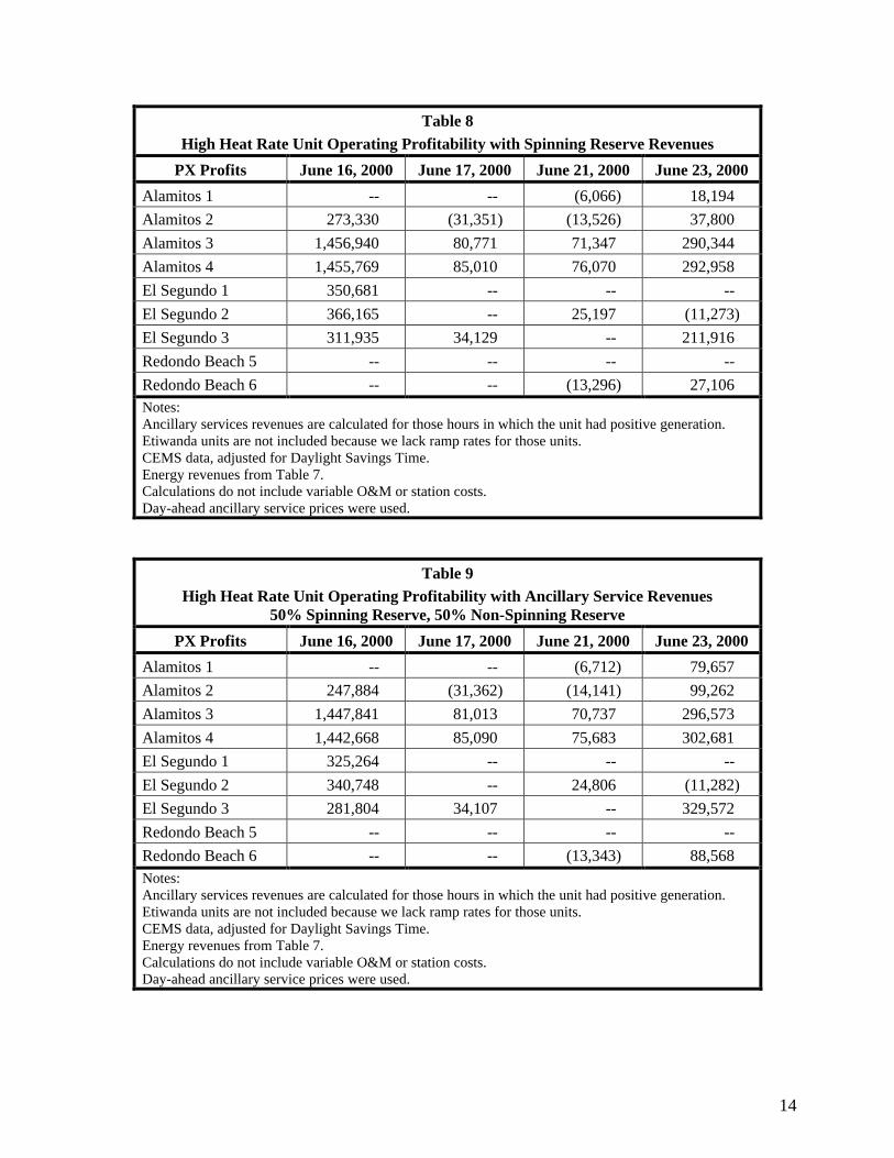
Overall, the dispatch of uneconomic units would have added over 1,000 MW of generation onevery day other than June 3 over the period June 1-11. Furthermore, the dispatch of uneconomicgeneration would have exceeded 4,000 MW on every day between June 4 and June 10, as shownin Table 14.

21

Table 14Simulated Output of Unprofitable Off-Line Units

Klein Capacity and Uncapped Prices

PX ProfitJune 1,

2000June 2,

2000June 3,

2000June 4,

2000June 5,

2000June 6,

2000June 7,

2000June 8,

2000June 9,

2000June 10,

2000June 11,

2000

Alamitos 1 Running Running Running Running Running Running Running 1,400 525 Off Off

El Segundo 1 Running Running -- -- 1,925 1,400 1,400 1,750 525 Off Off

El Segundo 2 525 -- -- -- Running Running Running 1,400 525 Off Off

El Segundo 3 Running Running Running Running Running Running Running Running Running 2,680 670

Etiwanda 1 396 -- -- -- 1,452 924 924 1,188 396 Off Off

Etiwanda 2 396 -- -- -- 1,188 924 924 1,056 396 Off Off

Etiwanda 3 -- -- -- -- -- -- -- -- 4,800 3,520 1,280

RedondoBeach 5 525 2,100 -- 1,925 1,575 1,225 1,225 1,400 350 Off Off

Total 1,842 2,100 0 1,925 6,140 4,473 4,473 8,194 7,517 6,200 1,950

Notes:(1) “Running” means unit was on-line for at least part of the day in the real world per the CEMS data, adjusted for Daylight Savings

Time.(2) “Off” means the unit was off-line in the real world and would not have been dispatched in any hour based on its incremental dispatch

price.(3) “Simulated Output” is the total calculated output for hours in which the SP-15 PX Price >= Dispatch price on days on which operation

would have been unprofitable over the day as a whole evaluated at day-ahead prices (per Table 13).

As before, the analysis of profitability we have undertaken is meant to be illustrative and doesnot provide a complete assessment of the profitability of operating these units in additionalhours. First, the calculations overstate revenues because they are based on Klein capacities,which measure gross output, not the net output that was available for sale. Second, no account istaken of deratings that might have prevented some of these units from operating at capacity (or atall) during this period. Third, the calculations assume all of the output could have been sold atday-ahead prices, which would not have been feasible under the California market design forpotentially marginal firms lacking perfect foresight.35 Fourth, the calculations do not takeaccount of ancillary service revenues.36 Fifth, the calculations take no account of CAISOdispatch instructions, ramp rates, or environmental output limits. Sixth, the calculations do notinclude any allowance for variable O&M. Seventh, the Klein heat rates may differ from theactual heat rates under these operating conditions.

To be clear, the point here is not that we have demonstrated that these units would surely beunprofitable. The point is that there is reason to believe the simulation of electric output basedon full load incremental heat rates without regard to minimum load costs, start-up costs, averageheat rates or physical unit constraints has the potential to dispatch significant amounts ofuneconomic generation and thereby systematically understate the competitive price level. 35 We address this point below.36 We also discuss this point further below.

22

Table 15 includes in this calculation of profits for the days June 1-11 the estimated ancillaryservice revenues of each unit from selling capacity in the spinning reserve market at day-aheadprices. It is again seen that units that would have been dispatched based on their incrementalheat rates would often have been unprofitable to operate taking minimum load costs intoaccount.

Table 15Hypothetical Profits for Off-Line Units Scheduled at SP-15 PX Prices Based on Incremental Heat Rates

Including Spinning Reserve Revenues at Day-Ahead Prices

PX ProfitJune 1,

2000June 2,

2000June 3,

2000June 4,

2000June 5,

2000June 6,

2000June 7,

2000June 8,

2000June 9,

2000June 10,

2000June 11,

2000






Notes:(1) “Running” means unit was on-line for at least part of the day in the real world per the CEMS data, adjusted for Daylight Savings Time.(2) “Off” means the unit was off-line in the real world and would not have been dispatched in any hour based on its incremental dispatch price

and the SP-15 PX price.(3) Profit calculations, by hour, summed over the day:

If SP-15 PX Price ≥ Dispatch Price then Full Load Revenues minus Full Load Costs (average heat rate).If SP-15 PX Price < Dispatch Price then Block 1 Revenue minus Block 1 Costs (average heat rate).

(4) Assumptions:Max Capacity = Klein Block 5 Capacity.Min Capacity = Klein Block 1 Capacity.Average heat rates from Klein.Gas Price = $4.99.Allowance Cost = $10/lb.Emissions rates per CEMS.PX prices are SP-15 zonal PX prices.

Spinning reserve revenues equal ten-minute ramp rate * SP-15 day-ahead spinning reserve price.

We also undertook the same calculation including reserve revenues assuming that 50 percent ofthe unit’s ramping capacity was sold as spinning reserve and 50 percent as non-spinning reserve.Once again, operation was often unprofitable if evaluated based on day-ahead prices and real-time schedules.

23

Table 16Hypothetical Profits for Off-line Units Scheduled at SP-15 PX Prices Based on Incremental Heat Rates

Includes Ancillary Service Revenues for 50% Spinning/50% Non-Spinning at Day-Ahead Prices

PX ProfitJune 1,

2000June 2,

2000June 3,

2000June 4,

2000June 5,

2000June 6,

2000June 7,

2000June 8,

2000June 9,

2000June 10,

2000June 11,

2000






Notes:(1) “Running” means unit was on-line for at least part of the day in the real world per the CEMS data, adjusted for Daylight Savings Time.(2) “Off” means the unit was off-line in the real world and would not have been dispatched in any hour based on its incremental dispatch

price and the SP-15 PX price.(3) Profit calculations, by hour, summed over the day:

If SP-15 PX Price ≥ Dispatch Price then Full Load Revenues minus Full Load Costs (average heat rate).If SP-15 PX Price < Dispatch Price then Block 1 Revenue minus Block 1 Costs (average heat rate).

(4) Assumptions:Max Capacity = Klein Block 5 capacity.Min Capacity = Klein Block 1 capacity.Average heat rates from Klein.Gas Price = $4.99.Allowance Cost = $10/lb.Emissions rates per CEMS.PX prices are SP-15 zonal PX prices.

Spinning reserve revenues equal ten-minute ramp rate (.5 * SP-15 day-ahead spinning reserve price + .5 * SP-15 day-ahead non-spinningreserve price).

Although in a well designed electricity market an on-line generator would always find it mostprofitable to offer all of its ramping capacity as spinning reserve, this would not be rational in theCalifornia electricity market. The combination of sequential clearing of ancillary servicemarkets and the “rational buyer protocol,” makes it unprofitable for a competitive on-linegenerator to offer all of its ramping capacity in the spinning reserve market at cost, but insteadrequires that generators structure their bids to guess the market clearing price.

E. Would Operation Have Been Profitable at Simulated Prices?

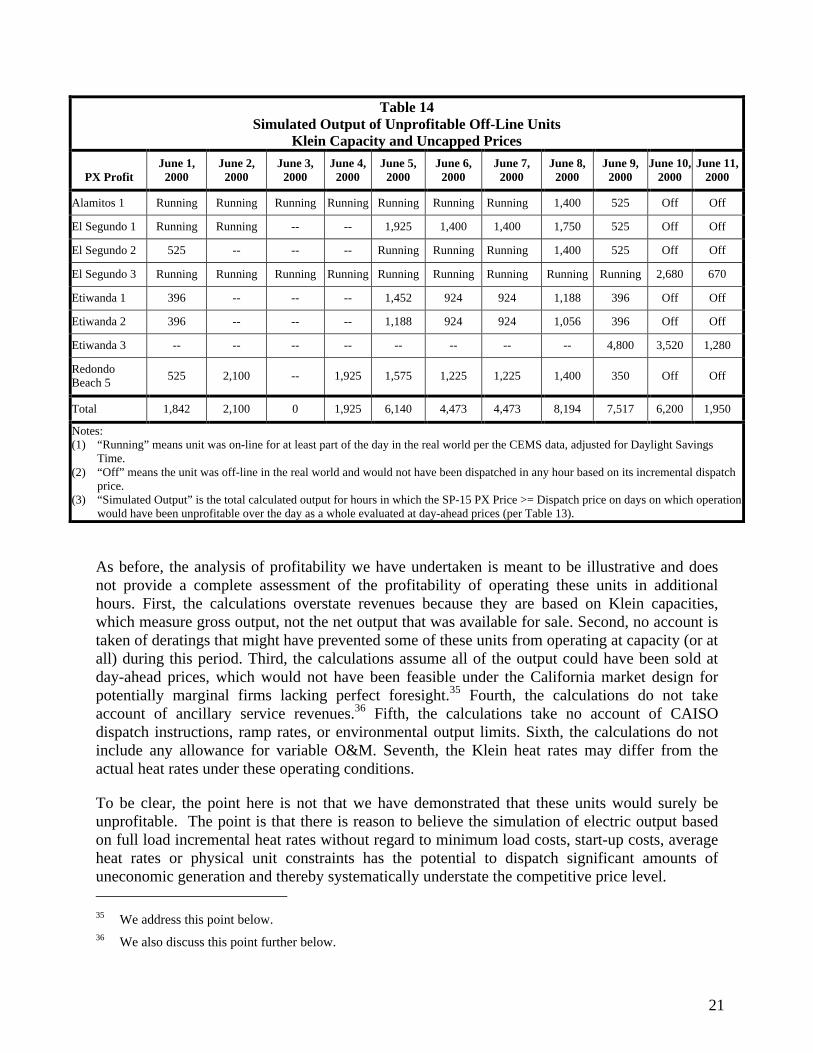
Now we turn to another question, for the units that were operating on high priced days in June,would their operation still have been profitable at the prices simulated by Joskow and Kahn?Joskow-Kahn also does not address this issue in the reply, instead assessing whether it wasprofitable for the plants that were actually operating in the real world to operate at real-worldday-ahead prices. The issue raised by their simulation results, however, is not the profitability ofoperating these plants at real-world prices, but whether these units would have been profitable tooperate at the simulated prices. As above, we cannot provide a full answer to this questionwithout the hourly prices simulated by Joskow and Kahn. We can, however, provide an

24

indication of the answer by capping real-world energy prices at $142.96/MWh37 and askingwhether all of the units that were actually operating on some of the high priced days would stillhave been profitable to operate. Table 7 above portrayed the profitability of operating the 13high cost units on June 16, 17, 21 and 23 excluding ancillary service revenues. There were sixinstances of days on which the six highest cost units operated but would have lost money basedon real-world PX prices. This profitability calculation has then been repeated with PX pricescapped at $142.96, approximating the price level simulated by Joskow and Kahn. It can be seenin Table 17 that there are an additional three instances (Alamitos 2 on June 16 and June 23;Redondo Beach 6 on June 23) of units that operated in the real world but would not have beenprofitable to operate at simulated prices.


Day-Ahead SP-15 Prices Capped at $142.96


Alamitos 1 -- -- (13,144) (10,296)

Alamitos 2 (5,218) (34,585) (20,502) (4,289)

Alamitos 3 348,634 79,746 65,164 193,455

Alamitos 4 348,084 83,242 72,084 194,953

El Segundo 1 33,396 -- -- --

El Segundo 2 38,911 -- 19,904 (12,230)

El Segundo 3 17,505 27,937 -- 117,004

Etiwanda 1 72,245 -- -- --

Etiwanda 2 56,070 -- -- --

Etiwanda 3 248,256 66,865 (998) 177,010

Etiwanda 4 215,765 51,400 (315) 183,192

Redondo Beach 5 -- -- -- --

Redondo Beach 6 -- -- (18,235) (19,370)Notes:CEMS heat rates.Gas Price = $4.99.Allowance Cost = $10/lb.Emissions rates per CEMS.Calculates are based on CEMS data, adjusted for Daylight Savings Time.Calculations do not include variable O&M or station costs, or potential ancillary services revenues.

37 If real-world PX prices were capped at $142.96/MWh, the average June PX price would be $74.03/MWh,

which is equal to the figure reported by Joskow and Kahn for their simulation model. We realize that this isonly a rough approximation of the prices they estimated, as our methodology likely reduces prices above$142.96 by more than they fell in the Joskow-Kahn simulation and reduces prices below $142.96 by less thanthey fell in the Joskow-Kahn simulation. Lacking access to the Joskow-Kahn simulation prices, this appears tobe a reasonable approach to illustrating the underlying conceptual issue.

25

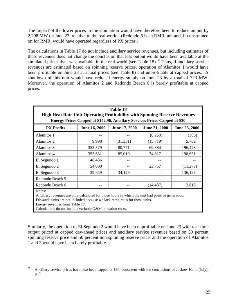
The impact of the lower prices in the simulation would have therefore been to reduce output by2,298 MW on June 23, relative to the real world. (Redondo 6 is an RMR unit and, if constrainedon for RMR, would have operated regardless of PX prices.)

The calculations in Table 17 do not include ancillary service revenues, but including estimates ofthese revenues does not change the conclusion that less output would have been available at thesimulated prices than was available in the real world (see Table 18).38 Thus, if ancillary servicerevenues are estimated based on spinning reserve prices, operation of Alamitos 1 would havebeen profitable on June 23 at actual prices (see Table 8) and unprofitable at capped prices. Ashutdown of this unit would have reduced energy supply on June 23 by a total of 723 MW.Moreover, the operation of Alamitos 2 and Redondo Beach 6 is barely profitable at cappedprices.

Table 18High Heat Rate Unit Operating Profitability with Spinning Reserve Revenues

Energy Prices Capped at $142.96, Ancillary Services Prices Capped at $30


Alamitos 1 -- -- (8,258) (305)Alamitos 2 9,998 (31,351) (15,719) 5,702Alamitos 3 353,579 80,771 69,884 196,428Alamitos 4 355,631 85,010 74,817 198,631El Segundo 1 48,486 -- -- --El Segundo 2 54,000 -- 23,757 (11,273)El Segundo 3 39,859 34,129 -- 136,128Redondo Beach 5 -- -- -- --Redondo Beach 6 -- -- (14,487) 2,815Notes:Ancillary revenues are only calculated for those hours in which the unit had positive generation.Etiwanda units are not included because we lack ramp rates for those units.Energy revenues from Table 17.Calculations do not include variable O&M or station costs.

Similarly, the operation of El Segundo 2 would have been unprofitable on June 23 with real-timeoutput priced at capped day-ahead prices and ancillary service revenues based on 50 percentspinning reserve price and 50 percent non-spinning reserve price, and the operation of Alamitos1 and 2 would have been barely profitable.

38 Ancillary service prices have also been capped at $30, consistent with the conclusions of Joskow-Kahn (July),

p. 9.

26

Table 19High Heat Rate Unit Operating Profitability with Ancillary Service Revenues

50% Spinning Reserve/50% Non-Spinning ReserveDay-Ahead Energy Prices Capped at $142.96, Ancillary Services Prices Capped at $30


Alamitos 1 -- -- (7,983) 63Alamitos 2 7,552 (31,362) (15,412) 6,070Alamitos 3 352,285 81,013 69,950 196,396Alamitos 4 354,043 85,090 75,007 198,722El Segundo 1 46,068 -- -- --El Segundo 2 51,583 -- 23,971 (11,282)El Segundo 3 37,005 34,107 -- 136,834Redondo Beach 5 -- -- -- --Redondo Beach 6 -- -- (14,058) 64,277Notes:Ancillary revenues are only calculated for those hours in which the unit had positive generation.Etiwanda units are not included because we lack ramp rates for those units.Energy revenues from Table 17.Calculations do not include variable O&M or station costs.

We reiterate that these calculations do not reflect the actual profitability of any of these units.These calculations do not reflect variable O&M costs, are based on gross, not net, output, valuereal-time output at day-ahead prices, and assume that unloaded capacity could have been fullyscheduled to provide ancillary services. The point of these calculations is directional, takingaccount of minimum load costs and operating inflexibilities can materially impact the calculatedprofitability of operating units to meet load, and simulations that ignore these costs may notsimulate the competitive equilibrium level of prices.

F. Does Market Design Matter?

A final point regarding these profitability assessments is that they illustrate the reality that theCalifornia market design is indeed an important issue in understanding generator biddingbehavior. In particular, the lack of three-part bids in the PX day-ahead energy market, separationof the energy and ancillary service markets, sequential clearing of the ancillary service marketsand lack of effective congestion management mechanisms either day-ahead or in real time, areall critical limitations of the California market design that have potentially substantial impacts onmarket outcomes. Joskow-Kahn asserts that market design is not part of the problem, statingthat:

“Finally, we may ask if the inefficient dispatch was somehow caused by theinefficiencies in the market design alleged by Harvey & Hogan. With the amountof daily capacity adjustment illustrated in Table 12, it seems difficult to argue thatgenerators were somehow prevented by market rules from turning on their

27

capacity when it was economic. The more plausible hypothesis is that generatorswere withholding at least some of the capacity listed in Table 13.”39

We disagree. The issue is, of course, not whether generators were prevented from turning ontheir capacity, but whether the market design facilitated or hindered efficient unit commitmentdecisions. As discussed more fully below, Table 12 in Joskow-Kahn does not actually provide agood indication of how much capacity was generally being turned on and off on a daily basis.Even if it did, however, this would not support a conclusion that market design is unimportant.The more capacity is potentially turned on and off every day, the more important it will be tohave an efficient market-based unit commitment process. This process must permit marketparticipants to ensure that the right units are turned on and off and that an efficient tradeoff ismade between the commitment of inflexible units with high start-up costs and low incrementalcosts and quick start units with higher incremental costs. Joskow-Kahn argues such problemsare immaterial.

We believe that several elements of the California market design are important in understandingCalifornia market performance. As Joskow has observed for the early operation of the Californiamarket:

"Flaws were identified in the congestion management system, with the contractsdesigned to mitigate local market power problems [footnote in original], theprotocols for planning and investment in transmission and the interconnection ofnew generating plants, the real time balancing markets, the ancillary servicesmarkets, under-scheduling before real time operations, and other areas. Thesemarket design flaws increased the costs of ancillary services far aboveprojections, led to scheduling and dispatch inefficiencies, slowed downinvestment in new power plants, increased the costs of managing congestion,increase spot market price volatility, and increased wholesale market pricesgenerally."40

It is unlikely that the analysis of the exercise of market power is immune from these generaldefects which continued in California through the period of study.

1. Three-Part Bids

First, the lack of three-part bids in the PX day-ahead market means that under the Californiamarket rules there is no bidding strategy (other than having perfect foresight) that would enablegenerators to bid in such a manner as to ensure that they are fully scheduled in the day-aheadenergy market when it is economic for them to operate, without risking being scheduled tooperate when it is not economic for them to operate. In the day-ahead markets coordinated bythe PJM and New York ISOs, a generator could submit cost-based three-part bids that wouldenable its unit to be fully scheduled, based on its bids, without risking uneconomic commitment.

39 Joskow-Kahn (July), p. 25.40 Paul M. Joskow, "California's Electricity Crisis," MIT Working Paper, November 2001, (forthcoming Oxford

Review of Economic Policy), pp. 21-22.

28

It is an explicit design feature of the CAISO market to make it impossible for generators to bid inthis manner.

As a practical matter, therefore, while a generator in PJM or New York lacking perfect foresightcan readily submit cost-based bids that ensure that their units would be fully scheduled at day-ahead prices and would sell additional output at real-time prices if real-time energy pricesexceeded day-ahead energy prices, this is not the case in California. The California marketdesign makes it likely that the marginal generators will not be economically scheduled in theday-ahead PX market and will potentially sell additional output in real time at prices that may belower than day-ahead prices. Thus, in calculating energy revenues in the examples above, weassumed for illustrative purposes that all of the real-time output had been sold at day-aheadprices or that all of the output that would have been profitable to sell at day-ahead prices couldhave been sold at day-ahead prices. While units that know they will be infra-marginal canaccomplish this by bidding their incremental costs into the PX market, there is no biddingstrategy that would permit marginal generators, such as those we have attempted to analyzeabove, to accomplish this, without risking being uneconomically committed at prices that do notrecover their costs.41 Moreover, one cannot assess the importance of this consideration byanalyzing the profitability of units committed on days on which the PX prices turned out to behigh, because part of the uncertainty is whether day-ahead prices will on average be high enoughover the day to recover the costs of operating or high only in a single hour.

2. Market Separation

A second and related problem is that this lack of any bidding strategy that would enable agenerator to offer capacity in a manner that ensures that it is scheduled to operate if it isprofitable but that it is not scheduled to operate unprofitably is further aggravated by theseparation of the energy and ancillary service markets. Like the New York electricity market,the California market has explicit ancillary service markets. Unlike the markets coordinated bythe New York ISO, however, the California energy and ancillary service markets are clearedsequentially. Marginal generators submitting bids into the California day-ahead energy marketsmust therefore also factor into their energy market bids a guess as to their likely ancillary servicerevenues. Failure to guess correctly that ancillary service prices would be high, could cause apotentially marginal generator to submit one part energy bids in the PX that cause it not to clearin the day-ahead market, despite day-ahead prices for energy and ancillary services that inretrospect would have made it profitable to operate.

3. Sequential Ancillary Service Markets

Even worse, the California day-ahead market design has a related third problem, that theancillary service markets themselves are cleared sequentially, and there is no cost-based biddingstrategy, and no bidding strategy at all other than perfect foresight, that would enable an on-linegenerator to bid so as to ensure that it is paid the market price of spinning reserves. The problem 41 Even units whose output has been fully sold in forward markets need to make a daily evaluation of whether it

would be lower cost to cover their forward sales by operating, purchasing power in bilateral markets or buyingpower in the spot market.

29

is illustrated by the spinning and non-spinning reserve prices for June 23 in our discussion above.Despite the fact that all spinning reserves satisfy the requirement for non-spinning reserves,capacity scheduled to provide spinning reserves was paid a substantially lower price day aheadthan capacity scheduled to provide non-spinning reserves on June 23. In order to capture thehigh non-spinning reserve prices that could have made it economic to keep a unit on line, agenerator had to hold capacity out of the energy market, and out of the spinning reserve market.Such a bidding strategy, of course, risks forgoing high prices in these markets in return for lowprices in the ten-minute market if there is no shortage in the ten-minute reserve market.42

In bidding into the day-ahead PX energy market, a generator would need to not only make anassessment of how to bid energy to avoid being uneconomically committed based on its one partbid, but also guess whether it should hold some capacity back to sell in the ancillary servicemarkets at higher prices, and then decide which ancillary service market it should offer itscapacity at what reservation price.

4. Congestion Management

Fourth, the CAISO market is confounded with inefficiencies and inconsistencies because of thelack of an effective congestion management system. Unlike electricity markets in PJM and theNYISO, the CAISO market design is intended to separate congestion management from theenergy dispatch. The effects of this poor market design have plagued the California market sincestart-up, and led the CAISO to increasingly rely on command and control, rather than markets, tomanage the system. These deficiencies had caused the FERC to find the CAISO’s congestionmanagement system to be “fundamentally flawed,” and direct reform, well prior to the summerof 2000.43

The lack of locational marginal pricing (LMP) led to amendment 19, that although ultimatelyrejected by the FERC, likely deterred the construction of the new generating capacity Californianeeded in 2001.44 Moreover, the zonal pricing system precluded development of an effectivereal-time congestion management system and produced a system in which California generatorswere being dispatched by both the Gen desk (zonal markets) and an RMR desk (intra-zonalcongestion management) leading to inconsistencies in both real-time dispatch and real-timepricing.

42 Moreover, such a strategy would require that the generator submit bids that would not be directly related to its

costs, making it at best difficult and possibly impossible to determine whether the generator was seeking toexercise market power or merely to be paid the market price. Scott M. Harvey and William W. Hogan, “Issuesin the Analysis of Market Power in California,” October 27, 2000 (hereafter Harvey-Hogan (October)), pp. 4-14.

43 FERC Docket No. ER00-555-000, January 7, 2000.44 Amendment 19 proposed to impose discriminatory charges and pricing systems on new generation built in

California in order to reduce “intra-zonal” congestion and avoid the need for LMP pricing. Amendment 19 wasdropped in January 2000 in response to FERC opposition, only a few months before the shortages began.

30

5. Bid Production Cost Guarantee

The bid production cost guarantee is a fundamental element of the electricity marketscoordinated by PJM and the NYISO but absent in California. The bid production cost guaranteeensures a generator that if it is dispatched or otherwise instructed by the system operator togenerate electricity, it will recover at least its as-bid costs, even if that generation turns out forsome reason to be uneconomic evaluated at settlement prices. This concept is applied to unitsscheduled to operate in the day-ahead market in the circumstance in which LMP market revenuesare insufficient to recover the units start-up, minimum load and incremental energy costs overthe day (which can be the case for units committed at the margin to provide reserves, to meetforecast load, or occasionally as a result of unit lumpiness). This concept is also applied to unitsinstructed to operate in real-time, in particular quick start units which, once started, must remainin operation for a period of time, even if electricity prices quickly fall below the units offer price.

The reasoning underlying the PJM and NYISO bid production cost guarantee is reliabilitydriven. If the system operator directs a generator to increase output, that generator should not beput in the position of needing to assess the likely profitability of following that dispatchinstruction and then deciding how to respond to the dispatch instruction. The lack of a similarbid production cost guarantee in California, and related elements of the CAISO overall real-timesettlements rules may have market as well as reliability impacts by at times reducing the supplyresponse to CAISO dispatch instructions and making the supply response in general lesspredictable by the CAISO.

6. Materiality of Market Design

Joskow-Kahn suggests that market design concerns are not material because they found that theoperation of the merchant units that actually operated was always profitable based upon day-ahead prices.45 But the argument does not support the conclusion. First, as discussed above, theoperation of these units would not always have been profitable even on the days that turned outto be high priced, if evaluated based on these hypothetical revenues.

Second, as noted above, part of the problem is that there is no bidding strategy that would enablegenerators to realize these hypothetical revenues. Both our calculations and those of Joskow andKahn illustrate what the generators would have realized had they been able to bid so as to selltheir output at day-ahead prices without being uneconomically committed (i.e., with perfectforesight). Their calculations do not show what the generators actually earned. The impact ofthe California market design would be seen precisely in the extent to which actual generator netrevenues are lower than calculated based on day-ahead prices. On days when real-time pricesare lower than day-ahead prices, our calculations could understate the profitability of generatorsthat operated but sold more in the day-ahead market than they generated in real time, but wouldoverstate the profitability of generators that sold less in the day-ahead market than they generatedin real time. Conversely, when real-time prices are higher than day-ahead prices, ourcalculations would understate the profitability of generators that sold less in the day-aheadmarket than they produced in real time, but would overstate the profitability of those that

45 Joskow-Kahn (July), p. 18.

31

operated but generated less in real time than they sold day ahead (as would be the case forgenerators that decided to close out unprofitable positions in the day-ahead market by purchasingpower in the real-time market).

Table 20 portrays the day-ahead energy and ancillary service prices for SP-15 during the on-peakhours of June 13. This is a day in which the day-ahead PX prices were relatively low but thereal-time prices were higher. The high real-time prices might simply reflect unexpected changesin weather conditions and have been unavoidable under any market design. The lack ofcentralized unit commitment and sequential markets for energy and ancillary services might alsohave contributed to the high real time price. It can be seen in Table 20 that while the PX prices,determined early in the day on June 12, averaged 114.24 for the 16 on peak hours, the price ofspinning reserve greatly exceeded the PX energy price in hours ending 11, 19, 20 and 21 andaveraged $109.48 for the on-peak hours. Furthermore, the price of non-spinning reserve greatlyexceeded the price of both energy and spinning reserve in hours ending 11-12 and 15-21,averaging $338.96 for the on-peak hours. This pattern suggests to us that the PX energy pricescleared at too low a price, possibly causing some units not to offer capacity for ancillary servicesor to offer capacity only at very high prices, with the capacity shortage showing up in non-spinning reserves. While it may be that every available unit was in fact committed on June 13,this is one type of situation in which the California market design may lead to inefficientoutcomes and inefficiently high prices.

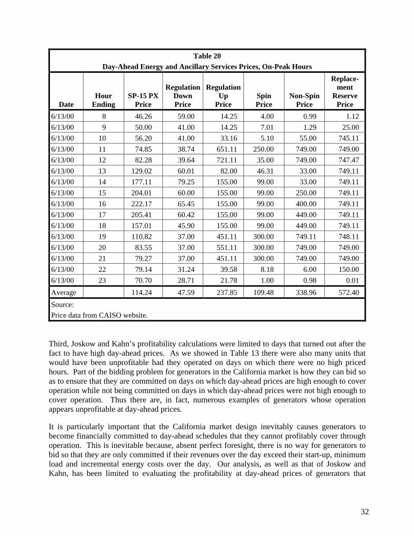
32

Table 20Day-Ahead Energy and Ancillary Services Prices, On-Peak Hours

DateHour

EndingSP-15 PX

Price

RegulationDownPrice

RegulationUp

PriceSpinPrice

Non-SpinPrice

Replace-ment

ReservePrice

6/13/00 8 46.26 59.00 14.25 4.00 0.99 1.126/13/00 9 50.00 41.00 14.25 7.01 1.29 25.006/13/00 10 56.20 41.00 33.16 5.10 55.00 745.116/13/00 11 74.85 38.74 651.11 250.00 749.00 749.006/13/00 12 82.28 39.64 721.11 35.00 749.00 747.476/13/00 13 129.02 60.01 82.00 46.31 33.00 749.116/13/00 14 177.11 79.25 155.00 99.00 33.00 749.116/13/00 15 204.01 60.00 155.00 99.00 250.00 749.116/13/00 16 222.17 65.45 155.00 99.00 400.00 749.116/13/00 17 205.41 60.42 155.00 99.00 449.00 749.116/13/00 18 157.01 45.90 155.00 99.00 449.00 749.116/13/00 19 110.82 37.00 451.11 300.00 749.11 748.116/13/00 20 83.55 37.00 551.11 300.00 749.00 749.006/13/00 21 79.27 37.00 451.11 300.00 749.00 749.006/13/00 22 79.14 31.24 39.58 8.18 6.00 150.006/13/00 23 70.70 28.71 21.78 1.00 0.98 0.01

Average 114.24 47.59 237.85 109.48 338.96 572.40

Source:Price data from CAISO website.

Third, Joskow and Kahn’s profitability calculations were limited to days that turned out after thefact to have high day-ahead prices. As we showed in Table 13 there were also many units thatwould have been unprofitable had they operated on days on which there were no high pricedhours. Part of the bidding problem for generators in the California market is how they can bid soas to ensure that they are committed on days on which day-ahead prices are high enough to coveroperation while not being committed on days in which day-ahead prices were not high enough tocover operation. Thus there are, in fact, numerous examples of generators whose operationappears unprofitable at day-ahead prices.

It is particularly important that the California market design inevitably causes generators tobecome financially committed to day-ahead schedules that they cannot profitably cover throughoperation. This is inevitable because, absent perfect foresight, there is no way for generators tobid so that they are only committed if their revenues over the day exceed their start-up, minimumload and incremental energy costs over the day. Our analysis, as well as that of Joskow andKahn, has been limited to evaluating the profitability at day-ahead prices of generators that

33

actually operated in real time. Generators that inadvertently become uneconomically committedat day-ahead prices in the PX will not necessarily operate in real time but may instead close outtheir position financially by buying power in the real-time market. The magnitude of the lossesthey incur relative to their schedule cannot be determined from publicly available data.

Fourth, apparently uneconomic commitment decisions at day-ahead prices may not always evenreflect generator decisions, as some of these units may have been committed by the CAISOunder RMR contracts. As noted above, Alamitos 4 and Redondo Beach 5 and 6 were all RMRunits and may have been committed on some days based on contract rather than market prices.

In fact, therefore, the Joskow-Kahn analysis provides no further information on whether thedesign of the California market led to inefficient commitment decisions.

G. Summary on Alamitos 2 and Similar Examples

Overall, rather than the Alamitos 2 example being in some sense artificial or misleading, itprovides a reasonable illustration of the principle that simulation studies that fail to account forstart-up costs, minimum load costs, and operating inflexibilities will meet load with generationresources that may not have operated profitably in the real world. As a result, such studies donot provide sufficient information regarding the competitive level of electricity prices. TheJoskow-Kahn simulations fall in this category. The simulations are suggestive of areas that needfurther analysis. But the simple simulation results do not dispose of the difficult empiricalproblems in analyzing the possible exercise of market power.

III. REVISED PRICE SIMULATION ANALYSES

Joskow and Kahn revise their simulation analysis and find that their conclusions are unchanged.While the revised paper addresses a few of the issues we have identified with simulation studiesof this type, the paper bypasses several of the major concerns we have previously identified andexacerbates, rather than addresses, others. In particular, Joskow-Kahn’s revised simulationanalysis does not take any account of start-up and no-load costs (and related unit inflexibilities),environmental output limits (other than emission allowance costs), models outages as uniformcapacity deratings and makes no allowance for the impact of deratings or similar outputlimitations. Moreover, the new simulations have new limitations arising from a materialunderstatement of real-world operating reserve requirements.

A. Start-Up and Minimum-Load Costs

Omitting start-up and minimum-load costs and operating inflexibilities from a simulation of theCalifornia or any other electricity market will tend to overstate the supply available at a givenprice in the high price hours (the simulated supply curve will be too flat) and will cause thesimulated prices to understate the competitive price level. As discussed above, Joskow-Kahnconsiders in the reply the profitability of the units that actually operated in the real world, butnever provide any theoretical or empirical response to the limitation we identify with pricessimulated assuming the absence of start-up and minimum costs and unit inflexibilities. Inparticular, they do not demonstrate or explain why the units dispatched to meet load in their

34

simulation model that were not operating in the real world, i.e., the incremental supply thatserves to reduce the simulated prices, would have been profitable to operate in the real world.The examples discussed above for June 1-11 and June 16, 17, 21 and 23 suggest the reverse.

The difference can be illustrated in terms of a conventional economic construct, the U-shapedfirm average cost curve (AC) portrayed in Figure 21. Having entered, the firm portrayed inFigure 21 might operate anywhere along its marginal cost curve (MC) in a particular period.Now suppose that this firm has not yet entered the industry, or in the metaphor of the electricindustry it has not started up. Is the minimum price at which it will supply output Pa or Pb? TheJoskow-Kahn approach assumes that the equilibrium price would be at Pa or below, as firms likethis would enter whenever the price rose above Pa, their lowest marginal cost. We assume thatthe equilibrium price could be as high as Pb, because firms would not enter (i.e., start–up) unlessthey expect to recover their average costs.

Figure 21

MC

AC

Pa

Price

Pb

Price

Quantity

Although Joskow and Kahn state that “We agree with the spirit of chronological analysis thatHarvey & Hogan introduced with their Alamitos 2 example. We present a more complete versionof our previous findings in this style.”46 But in the event, the simulation analysis is entirely non-chronological and ignores operating inflexibilities. In the Joskow-Kahn simulation, steam units


35

can start up at zero cost to serve load during a single high priced hour, then shut down, units thathave shut down can immediately restart, pumped storage units do not have to pump in the hoursbefore they use their water, hydro units can use their water in the highest load hours of the monthwithout regard to pondage constraints. All of these features reduce the cost of meeting load inthe simulation relative to the real world, but the difference does not reflect the absence of marketpower, only the absence of real-world operating inflexibilities.

The importance of start-up and minimum load costs were magnified during June 2000 bychanges in RMR contracts between 1999 and 2000. During 1999, 12,011 MW (based on Kleincapacities) of the units analyzed by Joskow and Kahn were designated as RMR units. During thesummer of 2000 this fell to 6,103 MW. We have seen indications that during 1999 the CAISOwas not only using the RMR contracts to manage intra-zonal congestion but was also using thesecontracts to put otherwise uneconomic units on at minimum load, thereby making their capacityavailable at incremental cost when needed during the day. The substantial reduction in theamount of RMR capacity available to the CAISO during the summer of 2000 would have limitedthe ability of the CAISO to manage prices by putting uneconomic units on line. Moreover, thedrop in RMR status was proportionately larger among the high cost units in the south discussedabove, with the RMR capacity falling from 2,929 in 1999 to 670 MW in 2000.

In addition, June 2000 was also the date at which the CAISO implemented pre-scheduling ofRMR units. Prior to June 2000, the CAISO determined RMR schedules after the PX cleared andthe CAISO cleared its day-ahead schedules, potentially leading to an inefficient unit commitmentbut permitting the CAISO to schedule additional RMR generation at minimum load to managethe real-time market based on the amount of energy that cleared in the PX or day-ahead bilateralmarkets. Beginning in June 2000, the CAISO determined day-ahead RMR schedules prior to thePX market and generators with RMR schedules were required to scheduled their energy in theday-ahead market, and could choose to be compensated at either contract or market (i.e., PX orbilateral) prices.47

B. Environmental Restrictions

Joskow and Kahn agree with our comment that cumulative environmental restrictions must betaken into account in analyzing CAISO prices and output, but suggest that these restrictions didnot impact the CAISO market until July or August and that environmental limits need not betaken into account in analyzing June prices. We agree that cumulative output limits were likelyless important in June than they became in later months but this is not the same as having noimpact. Units that had exhausted their annual hours of operation by July would very likely havebeen impacted by late June. Similarly, given the extremity of the constraints that AES hit later inthe year when AES was forced to shut down much of its generation because if cumulativeenvironmental limits, it is not obvious that those constraints did not begin to influence behaviorby late June. Reliable conclusions cannot be drawn from simulation models regarding the

47 Day-ahead LMP markets such as those coordinated by PJM and NYISO clear “intra-zonal” congestion neither

before nor after the energy market but simultaneously with the energy market. The CAISO was unwilling to dothis because it would have entailed adopting LMP pricing mechanisms. California loads and generators borethe costs of the resulting inefficiency.

36

exercise of market power as opposed to the impact of environmental limits if the environmentallimits are simply ignored in the simulation models. As we stated in our April paper:

“There is more than one way to model these environmental limits, and reasonablepeople will likely differ on the most appropriate approach. It may in fact bedesirable to simulate prices using a range of approaches to understand thesensitivity of the simulation results to these assumptions. It does seem clear,however, that it is not sufficient to simulate electricity prices for California in2000 under the assumption that none of these environmental limits existed.”48

More importantly, Joskow-Kahn does not address the impact on prices and output of environ-mental limitations other than cumulative output restrictions. In particular we noted that the DeltaDispatch restrictions are in effect on the Mirant steam units other than Potrero 3 and Pittsburgh 7specifically during the late May to early July period. Mirant can exceed the 86 degree limit onoutlet water temperatures only when directed to do so by the ISO, either in response to a state ofemergency or local area security (i.e., to operate at the level directed by the ISO under Mirant’sRMR contract). It is noteworthy that a number of the moderately high priced June days such asJune 12, 15, 16, 17, 21, 22, 23, and 30 did not have any hours of Stage 1 or higher levelemergency. We have obtained the Mirant real-time dispatch logs for several of these days (June15, 21, 22, 23 and 30). Although not all CAISO delta dispatch instructions are recorded in thelogs, it can be seen in the logs that even during some of the high priced hours Mirant receivedpermission to exceed the 86 degree limit only for its day-ahead RMR output and was notpermitted to operate at full output in many high-priced hours. For example, despite real-timeprices that reached $618.27 on June 22, Mirant appears to have been allowed to exceed the 86degree limit only for its day-ahead RMR schedule.

Prices would indeed have been lower in June 2000 if Mirant did not have to obey the 86 degreelimit, but that price impact reflects the environmental costs of operating at higher levels, notstrategic withholding by generators.49 Moreover, although little information appears to bepublicly available on other environmental limits, as we pointed out in the earlier paper, Mirantwas not the only generator subject to outlet water temperature restrictions.50

C. Reserves

A third major limitation of the Joskow-Kahn price simulations is a new one. In their priorsimulations, they described their simulation methodology as dispatching generation resources tomeet load and required reserves. We acknowledged in our April paper that this approach wassuperior to the BB&W/MSC51 simulation approach which does not account for real-world 48 Harvey-Hogan (April), p. 20.49 California PUC Decision No. 99-04-026, dated April 1, 1999. 1999 Cal. PUC Lexis 224.50 Harvey-Hogan (April), p. 22.51 See Severin Borenstein, James Bushnell and Frank Wolak, “Diagnosing Market Power in California’s

Restructured Wholesale Electricity Market,” August 2000 (hereafter BB&W) and Frank Wolak, RobertNordhaus, and Carl Shapiro, “An Analysis of the June 2000 Price Spikes in the California ISO’s Energy andAncillary Service Markets,” September 6, 2000 (hereafter MSC).

37

reserve requirements. We noted, however, that the simplified approach to reserve modelingtaken by Joskow and Kahn (i.e., treating reserves as load) could overstate market prices duringnon-shortage conditions.52

This methodology is radically changed, however, in simulations described in Joskow-Kahn(July). In the reply, Joskow-Kahn states that their new simulation takes account of only the 3percent regulation up requirement and assumes that the CAISO would not need to meet WSCCcriteria for minimum operating reserves.53 The justification of this approach appears to rest onthree grounds. First, that there was sufficient capacity available on unloaded hydro and GTs toprovide the required reserves.54 Second, that it is not necessary for the CAISO to maintainreserves in excess of its upward regulation margin. Third, that there was more than adequatecapacity outside California to cover CAISO reserve requirements. We discuss this reasoning indetail below. The bottom line is that because of this assumption Joskow-Kahn simulated amarket that is substantially different than that in which the CAISO operated. Market priceswould have been lower in such a market, but the lower prices would have nothing to do with theconduct of generators. This is symptomatic of a problem in using the differences betweensimulated and real-world prices to draw conclusions about competition. Unless the simulation isvery carefully calibrated against the real world, the differences between simulated and real-worldprices will simply reflect the differences between the simulation and the real world, notdifferences in competitive conditions.55

Consider the first of the rationales Joskow-Kahn offer for the new approach, that there wassufficient capacity available on unloaded hydro and GTs to provide reserves, without backingdown generation.56 If this proposition could be shown to be factually correct, then it wouldindeed be the case that it would have been unnecessary to carry reserves on steam units andreserve prices would have been determined by the bids of the hydro suppliers and GT units.Joskow-Kahn does not establish the validity of this proposition, but merely assert it. We wouldbe surprised if this were true. We know from the Mirant data that spinning and non-spinning

52 Harvey-Hogan (April), pp. 16-17.53 Joskow-Kahn (July), p. 7. They also state that “In our previous estimate, we followed Hildebrandt (2000) by

adding 10% to the observed demand to satisfy AS requirements. Harvey and Hogan agree with our currentview that this is too high (pp. 16-17).” What we actually said was that the Joskow-Kahn procedure:

“should correct for the considerations discussed above [downward biases in other studies], permitting theanalysis to identify capacity shortage hours and avoid the potential understatement of the market price ofenergy. In fact, this approach would have the potential to cause the simulation to overstate the competitivemarket price of energy because it would implicitly assume that all reserves are provided by infra-marginalgeneration which would also be an inaccurate assumption.” Harvey-Hogan (April), p. 16.

54 “We argue that unloaded hydro and extra-marginal peaking units are sufficient to meet the demand for otherancillary services.” Joskow-Kahn (July), p. 7. “We argue instead that most AS demand can and should beprovided by unloaded hydro capacity,” p. 8

55 It was explained to us long ago that direct comparisons between simulated and real-world prices would not bemeaningful, even using complex simulation tools that take account of start-up costs, no-load costs, unitinflexibilities, and transmission constraints, and even when the world being simulated is one based on regulatedcost-based offers.

56 “There is enough hydro in the California ISO control area to provide most of these services, both in reality andin our modeling of the energy market.” Joskow-Kahn (July), p. 8.

38

reserves were at times scheduled for the Mirant units, so these other resources must not alwaysbe sufficient even in NP-15. Moreover, we understand that the GT capacity was assumed to beavailable to be dispatched to meet load as well as provide reserves in the Joskow-Kahn model.This assumption in effect therefore potentially double-counts capacity, by assuming that it isavailable to generate energy and to provide reserves. To the extent that the simulation dispatchesthese units to meet load in the same hours in which Joskow-Kahn are assuming that these unitswere unloaded to provide reserves, the simulation double-counts capacity.

Joskow and Kahn’s second rational for ignoring reserve requirements is perhaps related andappears to us to reflect a misunderstanding of reliability criteria. Joskow and Kahn state that:

“Our analysis adopts a de-rating approach to forced outages, meaning that thecapacity we assign to all units is reduced by the assumed forced outage rate.When we stack up resources against demand, we are assuming that theseresources meet not only the final demand, but also the ‘outage loads’ associatedwith the expected level of forced outages, to the extent that outages occur on-the-day and are unknown ahead of time. These forced outages are the reason that ASreserves other than Regulation exist in the first place. In our procedure, we arealready including the effect of these ‘dispatched’ AS reserves on energy prices.Therefore, we add only 3% to demand for Regulation Up. This is similar in spiritto the arguments made by Borenstein, Bushnell and Wolak (BBW) for adjustingdemands to reflect Regulation Up but not other ancillary services in this type ofsupply curve analysis.”57

These are not the WSCC rules followed by the CAISO. WSCC rules require maintenance of 5-7percent operating reserves, and if the reserves are used to meet load, they require that reserves berestored within 60 minutes.58 In other words, under the WSCC rules for the idealized case with1000 small 1 MW plants and an average outage rate of 10 percent, the 900 MW of availableplant would be sufficient to meet approximately 810 MW of load, leaving 3 percent needed forup regulation and 7 percent for operating reserves. The Joskow-Kahn assumption implies thatthese same plants could meet 870 MW of load, needing only the 3 percent up regulation. In theless than idealized case with large and heterogeneous plant sizes, the difference between theWSCC rule and the Joskow-Kahn assumption could be even greater.

Joskow and Kahn’s simulations, in effect, assume that the reserves must be maintained as long asit is costless, but not if it becomes expensive. This assumption will also reduce simulatedelectricity prices as 5-7 percent less capacity would be needed to meet load. This reduction inelectricity prices would be appealing but it would have nothing to do with competition or theexercise of market power, and the grid is not operated in this manner for reliability reasons. Wepreviously explained at length why this same methodology as adopted by BB&W and MSC wasat odds with the actual CAISO and WSCC reliability standards.59 The system operator needs to 57 Joskow-Kahn (July), pp. 7-8.58 WSCC Minimum Operating Reliability Criteria, p. 3 “Restoration of operating reserves. After the occurrence

of any event necessitating the use of operating reserve, that reserve shall be restored as promptly as practicable.The time taken to restore reserves shall not exceed 60 minutes.”

59 See Harvey-Hogan (October), pp. 20-25.

39

have enough capacity to meet WSCC/NERC reliability targets after sustaining normal overnightunit losses and will take actions in real time (including expensive energy purchases) to restorereserves used to meet unexpected load or respond to contingencies.

We do not question that WSCC and CAISO prices would be lower if it were necessary only tomaintain sufficient reserves to account for load uncertainty, rather than to maintain reliabilityafter loss of generation units. Indeed, we discussed in prior papers how the WSCC and CAISOreliability standards contributed to high prices, but this impact is not a result of the exercise ofmarket power.60 Joskow and Kahn are at best simulating the operation of the grid under analternative set of reliability criteria. This is an exercise in simulating prices in a more benignenvironment in which units politely suffer proportionate outages on each day and it is notnecessary to maintain reserves to cover the loss of large generating units (because they are notlost all at once but only in proportion to their fixed outage rate). These modeling results mayhave little to say about the existence or exercise of market power, but merely demonstrate thatelectricity prices would be lower in this more benign environment.

Joskow-Kahn’s third reason for ignoring reserve requirements is the view that there are sufficientresources available outside the CAISO control area to meet CAISO reserve requirements. Inparticular, they note that “There are adequate resources in the region to meet these reserve needs.Resources available for reserves outside of the ISO control area include BPA, LADWP’s Castaicpumped storage plant (1,200 MW), and out-of-state gas turbines. Since BPA has adequatecapacity (if not energy) for the winter in the Northwest, then it should have had at least severalthousand MW in the Summer to sell as AS reserves.”61

The actual supply of reserves from outside the CAISO control area has not matched thischaracterization. If Joskow-Kahn were correct regarding the available supply of reserves fromoutside the CAISO control area, the limited supply of external reserves in the real world wouldsuggest that the source of the high prices in California was withholding of reserves by BPA andother external suppliers, rather than the claimed withholding by California generation owners.Alternatively, perhaps the problem is that the Joskow-Kahn assertion that BPA and others shouldhave had several thousand MW of excess reserves in the summer is inaccurate and fails to reflect1) the use of capacity to supply energy to California, 2) the need for BPA and other externalcontrol areas to maintain their own reserves at WSCC levels, 3) the impact of low hydroconditions on available capacity. In addition, the CAISO market design which treats spinningreserves as just another energy source to be dispatched to meet load, rather than as capacityreserved to respond to contingencies, may have driven energy limited resources out of theCalifornia reserve market during the summer of 2000, reducing the supply of reserves.

This is illustrative of the difficulties with such simulations that are at odds with the actualoperation of the electric system and introduce substantial differences between the simulatedworld and the real world that are unrelated to competitive behavior of thermal generators withinthe CAISO control area. Furthermore, it is noteworthy that no sensitivity analyses were under-taken of these important assumptions regarding reserve requirements that in effect increase the

60 Harvey-Hogan (October), pp.25-26.61 Joskow-Kahn (July), p. 8.

40

capacity available to the CAISO in shortage hours by between 5 and 7 percent, or a few thousandMW.

D. Outages

We pointed out in our April paper that the Joskow-Kahn treatment of generation outages asproportional deratings of capacity, rather than probabilistic outages, would tend to reduce thenumber of shortage hours and thus understate the competitive level of prices.62 In addition,because their methodology is based on assumed theoretical outage rates, rather than the actualoutage rates during the summer of 2000, the analysis cannot distinguish between “high pricesdue to the exercise of market power or to higher than assumed outage rates.”63 We alsoquestioned whether their simulation analysis included various thermal units owned by PG&Ethat were not available during all or part of the summer due to outages. Joskow-Kahn states thatthey responded to our comments about the Hunters Point units by deleting the unavailable PG&Eunits from the simulation64 but they do not appear to have addressed the more fundamentalobservations regarding the outage methodology employed in their simulation.

The treatment of outages as proportional deratings of capacity would be particularly likely tounderstate the competitive price level in periods of capacity shortage, when the market is likelyto be clearing on a highly convex portion of the industry inverse supply curve, as was often thecase in June 2000. Moreover, the impact of modeling of generation outages as proportionatederatings is unambiguously to understate prices.65 The impact of the second limitation isambiguous, because it is not know exactly what “historical outage rates” were used in thesimulation or what actual outages were in June. Joskow and Kahn refer to “HESI data on forcedoutage rates,”66 but it is not entirely clear which particular outage data are referenced.67 TheHenwood data also do not account for the minor operational problems that reduce real-worldoutput but may not amount to deratings. For example, the output of Mirant’s Potrero 3 unit hadto be reduced at times because the hydrogen used to cool the generator windings exceeded itstemperature limit, requiring a reduction in output to reduce the load on the cooling system. Thiscould happen as a result of a variety of problems in the cooling system, including warm baywater temperature and low tides. This is neither a forced outage nor a derating, but output isreduced.

62 Harvey-Hogan (April), p. 34.63 Harvey-Hogan (April), p. 33.64 Joskow-Kahn (July), p. 11.65 Paul L. Joskow and Edward Kahn, “A Quantitative Analysis of Pricing Behavior in California’s Electricity

Market During Summer 2000,” March 2001 (hereafter Joskow-Kahn (March)) , p. 13, states this procedure is“common” and “reflects standard industry practice.” Our experience is that the standard industry practice in realproduction simulations is to use some random process to generate a set of outages, which is why thecommercial production simulations, such as GE-MAPS, have such a feature.

66 Joskow-Kahn (March), p. 13.67 Joskow-Kahn (December) refers to the used of GADS equivalent forced outage data, which includes an

adjustment for deratings.

41

Joskow-Kahn suggests that its analysis of withholding somehow addresses whether the outputgap is due to withholdings or outages:

“In the absence of unbiased review of generators’ operating decisions, ourwithholding analysis is designed to answer an indirect question: Is the amount ofunavailable generation in the California market consistent with the amount wewould expect to be unavailable for engineering and other known reasons? Ourmeasures of the output gap show that these amounts are not consistent. As wehave calculated it, the output gap shows the amount of unavailable generationabove and beyond what would be expected if historical outage rates held true.”68

This does not appear to be the case, however. As far as we can detect, and based on our replica-tion of the withholding analysis, Tables 8 and 15 in the recent paper include no allowance for“historical outage rates,” and no allowance for total expected deratings, under generation andforced outages based on historical data for these or similar units at similar utilization rates.

E. Other Features of the Model

1. Load Shape

We pointed out in our April paper that the Joskow-Kahn use of hourly deciles could potentiallymaterially affect the estimated prices. In Joskow-Kahn (July) the new simulation uses 100 hourlyintervals as well as 10.69 It can be seen in Table 3 of Joskow-Kahn (July) that more accuratelyrepresenting demand and capturing the peaks increased the average price in the simulation bynearly $20 in June 2000 at a $10/lb. NOx price. This appears to us to be a material effect andsuggests that factors affecting the relative tightness of the market in the high priced hours canhave material impacts on estimated prices.70 The sensitivity results suggest that taking account ofreserve requirements would materially change the simulated results.

2. Hydro and Geothermal

We pointed out in April that it was uncertain whether the 8,000 MW of hydro power assumed tobe available in Joskow and Kahn’s original simulation analysis were actually available in everyhour of the four high load deciles, i.e., 40 percent of all June hours.71 In the new simulation,Joskow-Kahn raises the amount of hydro assumed to be available in the four high load deciles to8,500 MW based on their conclusion that 8,500 MW of hydro generation appears to have been

68 Joskow-Kahn (July), p. 6.69 This is the only sensitivity analysis presented in the study.70 As discussed below in Section III.E.3 below, some of the results based on the 100 hourly intervals are a bit

“odd,” suggesting that either the methodology is not quite as described or that there is something wrong withthe simulation results.

71 Harvey-Hogan (April), pp. 40-42, and Joskow-Kahn (March), pp.11-12, 34.

42

available on August 16, 2000.72 The figure on which they base their conclusion is calibratedonly to 2,000 MW, and hydro is the difference between two other regions, so it is hard to be surewhat quantities are being reported.73 It is not clear to us whether the actual peak hydro availableon August 16, or in June, was 8,500 MW, 8,000 MW or 7,500 MW. Were all 8,500 MW ofhydro available in all of the high-load decile hours in June (i.e., 40 percent of all hours)? Ninehours during August 16 were in the top load decile for the month and 14 hours were in the topfour deciles. The non-chronological Joskow–Kahn simulation apparently assumed that 8,500MW of hydro and pumped storage was available in all 14 of these high load hours. In practice,prices exceeded $155 during all 14 of the high load hours on August 16, yet the CAISO data towhich Joskow-Kahn refers do not indicate, to us, that 8,500 MW of hydro was available in these14 hours. Our point remains valid. Because the Joskow-Kahn simulation is based on assumedhydro output levels, it cannot provide evidence that market power was exercised, but onlyestablish that the price levels are consistent with either the exercise of market power, or lowerlevels of hydro output than assumed in the simulation. Moreover, since there is no reportedsensitivity analysis regarding the assumed hydro outputs, it is not known how sensitive thesimulated prices are to variations in the level of available hydro power.74

There is a similar ambiguity in the level of geothermal output assumed in the simulation.Joskow-Kahn based geothermal output on derated output capacities in their new simulation, butit is still not known how this output level compares to actual output.75 As above, we cannot tellfrom the analysis whether the simulated price levels are lower than real-world price levelsbecause of market power, or because of incorrect assumptions regarding the availability ofgeothermal energy. There is a similar ambiguity regarding the output of non-wind qualifyingfacility (QF) plants whose output also varies dramatically day to day and hour to hour.76

We observed in both of our prior papers discussing California price simulations that treatingenergy limited hydro and geothermal resources as price taking, rather than price making couldcause the simulation to estimate lower prices than prevailed in the real world, even if no marketpower were exercised and all thermal generation had been bid into the market at competitiveoffer levels and was fully dispatched.77 Joskow-Kahn did not change this feature of the model,nor offer any rationale for the approach taken.

3. Dispatch Instructions

We also pointed out in prior papers that simulations are not impacted by real-world constraintssuch as ramping limits or the chaos of real-time events.78 In the real world, electricity demand 72 Joskow-Kahn (July), p. 9. We have been unable to confirm with CAISO that only California hydro is included

in the shaded region referred to by Joskow and Kahn.73 California ISO CAISO 2001 Summer Assessment, Figure I-A, p. 9.74 It is also not known if the simulation took account of the need for pumped storage to consume energy off-peak.75 Joskow-Kahn (July), p. 10.76 California ISO CAISO 2001 Summer Assessment, p. 13 , and Figure II C, p. 1477 Harvey-Hogan (October), p. 34-35; Hogan-Harvey (April), pp. 22-23.78 Harvey-Hogan (October), p. 28 and Harvey-Hogan (April) pp. 60-64.

43

must be met on a short-term basis and system operators sometimes must meet load with high costquick ramping generation at the same time that generation with lower bids is on-line, and slowlyincreasing its output. In the Joskow-Kahn non-chronological simulation, there are no rampingconstraints and load can always be met with the cheapest available generation. Similarly, even ifstart-up and minimum load costs are taken into account in the determination of equilibriumprices, real-world prices are also impacted by the fact that the actual demand level is oftendifferent from the anticipated level, which can require that load be met with much moreexpensive than anticipated generation. If the inverse supply curve is convex, these errors willnot cancel out and demand uncertainty will raise the equilibrium level of real-time prices.79

Moreover, Joskow and Kahn simulate the least cost dispatch of generation to meet load, ratherthan attempting to simulate the operation of a market with the CAISO rules. Any marketinefficiency arising from California market design would therefore be classified as arising fromthe exercise of market power.80 None of these considerations are addressed in the Joskow andKahn’s reply.

4. Transmission Congestion

We also pointed out in our prior paper that the Joskow-Kahn simulation assumed the absence oftransmission constraints within California.81 The new Joskow-Kahn simulations apparentlycontinue to assume the absence of transmission constraints, and the comparisons between thesimulated and PX prices continue to be based on the “unconstrained” PX price. The “uncon-strained” PX price is a price calculated as if there is no inter-zonal congestion, based upon actualbids, which may have been submitted in a period in which there was inter-zonal congestion. It isnot the actual settlement price. The importance of this assumption is not clear. However, it maybe of less importance given that we are unaware of arguments that transmission constraintsplayed a prominent role in high priced hours in California in 2000.

5. Imports

We previously expressed concern with the ambiguously described methodology for accountingfor imports in the BB&W, MSC and Joskow-Kahn simulation studies.82 This methodology hasnot been clarified. Moreover, we have separately pointed out that the import elasticity assumedby Joskow-Kahn implies a much lower price response for import supply than internal CAISOsupply.83 Our concern regarding the validity of the import modeling is exacerbated by the newJoskow-Kahn results and discussion. It can be seen in Table 3 in Joskow-Kahn (July)(reproduced below as Table 22) that the simulated price for June 2000 declines with increases in 79 Harvey-Hogan (April), p. 38-40.80 Harvey-Hogan (October), pp. 29, 31-34, and Harvey-Hogan (April), pp. 35-36.81 Harvey-Hogan (April), p. 23-25.82 Harvey-Hogan (October), p. 35-36; Harvey-Hogan (April), p. 21, and Harvey-Hogan (November), pp. 18-25.83 See Harvey-Hogan (November) pp. 20-25, particularly Table 7. The assumed import elasticity will not bias the

simulation results as long as simulated imports equal actual imports at the real-world price. The assumedimport elasticity can, however, magnify the impact of other elements of the simulation that overstate supply.

44

NOx allowance costs above $10/lb. We do not find this plausible and it is tempting to assumethat is just a typographical error. The Joskow-Kahn paper, however, notes the anomaly andexplains:

“The June results for the 100 load point estimate are somewhat counter-intuitive,with benchmark prices first rising as RTC prices go from $0/lb to $10/lb and thenfalling as these prices go from $10/lb up to $30/lb. The lower price at high RTCcosts is due to the import elasticity effect, which brings in more resources as in-state fossil costs increase. These increased imports then reduce the effect of the$750/MWh price cap as well.”84

If the anomalous results in Joskow-Kahn Table 3 are attributable to the supply of imports, thisimplies that the import supply curve underlying these simulation results makes more importsupplies available at lower prices ($71.65 for example) than at higher prices ($74.03). Thissuggests to us that there is something else driving this simulation beyond what has beendiscussed above.85

84 Joskow-Kahn (July), p. 12, footnote 26.85 An alternative explanation might be that the prices in Joskow-Kahn Table 3 (p.13) are averages calculated using

a set of weights that depends on the amount of thermal generation dispatched. If this is the case, they are notcomparable to the PX prices to which they have been compared. A paper released just as we were completingthis paper, Paul Joskow and Edward Kahn, "A Quantitative Analysis of Pricing Behavior in California’sWholesale Electricity Market During Summer 2000," December 21, 2001, p. 17 (hereafter Joskow-Kahn(December)), contains simulation estimates that have the expected pattern, i.e. they increase with NOx costsand differ materially from those in Joskow-Kahn (July). There is no explanation for these differences.

45

Table 22Joskow-Kahn Table 3

Summary of Benchmark Costs

Average MC ($/MWh)

Month

AveragePX Price($/MWh) $0/lb $10/lb $20/lb $30/lb $35/lb

100 Load PointsMay 47.23 55.78 59.38 60.54 62.20 62.85June 120.20 70.81 74.03 71.65 62.66 64.16July 105.72 56.23 54.80 56.69 58.26 59.04August 166.24 64.88 69.58 72.75 75.59 78.13September 114.87 68.96 72.47 75.35 78.26 79.67

10 Load PointsMay 47.23 44.01 45.81 48.49 50.37 51.34June 120.20 52.01 53.98 56.70 58.04 59.24July 105.72 48.31 50.30 51.91 53.90 54.38August 166.24 60.86 64.46 68.47 72.79 74.74September 114.87 66.41 70.77 74.06 76.58 77.51

Source:Joskow-Kahn (July), Table 3, p. 13.

This highlights a general problem with the simulation. The simulation shows that high prices inreal system were due to market power, or due to the simulation using lower reserve requirementsthan applied in the real system, and/or ignoring start-up and no-load costs, and/or treating forcedoutages as proportional deratings and ignoring maintenance outages and other operating outputlimitations, and/or ignoring environmental output limitations, and/or overstating hydro, QF,geothermal and/or import supply. This simulation comparison is not easy to make, and thearguments above suggest that with the available data we cannot assume that these differences donot matter enough to change the conclusion about the size and scope of the exercise of marketpower.

F. Simulations

It is not an easy matter to design an efficient market for an electricity system. Furthermore, it isnot a simple matter to simulate a market as complex as the electricity system, especially one withbadly designed market institutions. Some of the problems with the Joskow-Kahn simulations arenormally avoidable, some perhaps avoidable with effort, and some are intractable. However, ourexperience has been that even answering simpler questions than that posed by Joskow-Kahn canbe difficult and resource intensive.

46

The failures to take account of start-up costs, minimum load costs, unit inflexibilities, andtransmission constraints are correctable. Because these considerations have such powerfuleffects on simulation results, standard industry simulation tools used for many years have beendesigned to address these problems. GE MAPS, for example, is a widely used simulation tool inthe electricity industry.86 MAPS is a chronological model; that is, it looks at each hour insequence, and runs a unit commitment evaluation on a weekly basis and then dispatchesgeneration to meet load given this unit commitment. MAPS has a 3-pass option for the unitcommitment step, which takes longer to run but provides a more consistent unit commitment.Because MAPS is chronological, it can and does take account of inflexibilities such as minimumrun times in its unit commitment. MAPS also takes account of transmission constraints indispatching generation to meet load and even calculates LMP prices for each location specified.Most standard industry modeling tools, including GE MAPS, are also designed to take accountof reserve requirements, although it is sometimes not possible to model all of the locationalrequirements applying to each category of reserves. Data on non-dispatchable generation byQFs, wind and other generation sources can readily be built into the model and the othergeneration dispatched based on start-up, minimum load, and incremental energy bids.87

Most simulation studies, however, are intended to simulate future prices and compare alternativemodeling scenarios, rather than to replicate past prices. This focus on the differences in modeledscenarios necessarily controls for the other common features of the model and isolates the causesof the differences. By contrast, it is quite another matter to extend this simulation approach tocompare the model to the real data, especially under highly stressed conditions. One could inprinciple build in hourly load patterns and unit outages (if one had the outage data) reflecting theactual historical outages. Alternatively, as noted, one could build in outage factors reflectingforced outages and deratings and let MAPS apply these factors on a random basis.88

It would be much more difficult to build in environmental limits, even if one had all of therequired data. Monthly and annual energy limits are hard to model, and capacities that changehour to hour during a day and depend on the status of the system (such as the Delta Dispatch)would not be easy to model in MAPS. One could perhaps indirectly model the Delta Dispatchby including the capacity with a very high dispatch price to signify that it would only becomeavailable for dispatch during shortages in which the price was high, but this would not capture allof the complexities of the Delta Dispatch.

Price setting hydro, pumped storage and geothermal generation could also be modeled in MAPS,but if they are modeled as price setting, they cannot be modeled as energy limited, and if they are

86 GE MAPS can be licensed from GE Power Systems Economic Consulting or GE will run MAPS simulations

for the user. GE Power Systems Economic Consulting has existing transmission databases for all U.S. regions,including the WSCC, as well as generation data bases, based on publicly available data. There also a variety ofspecialized MAPS databases for various regions that included various confidential data that are available for useby certain entities. Many MAPS users begin with the GE databases and modify them based on theirinformation.

87 The bid curves in MAPS may have up to seven price points.88 This approach has the property that the results depend on the actual pattern of random outages. We have found

that even average annual prices can be noticeably affected by the pattern of outages. For this reason, oneusually uses the same random number seed in comparative MAPS runs.

47

modeled as energy limited, they cannot be modeled as price setting and the outcome of thesimulation might depend to a considerable degree on the assumed bidding strategy of theseentities.

Further, the existing structure of most simulation tools is not well suited to modeling the chaos ofreal-time. While MAPS and other simulation tools include unit ramp rates, there are no surprisesin the current structure. The load shape on which the unit commitment is based is also the loadshape against which the units are dispatched. Moreover, random outages all occur prior to unitcommitment in MAPS. This is similar to the way Joskow and Kahn have treated outages butwith such an approach there is no analogue to the forced outage occurring in real-time.

While people have talked of modifying this structure, it has not to our knowledge actually beendone, and entities using simulation tools make other ad hoc adjustments to the simulated pricesto reflect these elements of the real world.

Finally, it should be noted that MAPS dispatches generation to meet load at least cost andcalculates LMP prices based on this dispatch. This is not the structure of the CAISO markets. Asimulation model would need to be modified to account for the dispatch of RMR generation bythe CAISO and intra-zonal congestion management. Moreover, a substantial effort might berequired to translate the dispatch of generation to meet load in MAPS and the resulting LMPprices, into a set of zonal prices as they would be calculated by the CAISO. It is not apparentthat there is a straight-forward way in which to reflect the structure and inefficiency of Californiaelectricity markets in a simulation.

IV. WITHHOLDING ANALYSIS

A. Introduction

In our April paper we replicated the Joskow-Kahn withholding analysis and observed that muchof the apparent output gap was attributable to several factors:

1. The hours selected by Joskow-Kahn for the “output gap” analysis included hours with highday-ahead prices but low real-time prices. Competitive firms should be expected to operatebelow capacity when real-time prices are low, regardless of day-ahead prices.89

2. The data on ancillary services utilized by Joskow and Kahn measured ancillary servicesprocurement from internal CAISO generation, not requirements, and did not include all ofthe zones included in the withholding analysis. In addition, ancillary service procurementfrom internal CAISO generation was higher in the high real-time priced hours.90

3. Some of the hours with high day-ahead and real-time prices were immediately before or afterlow priced hours or dispatch intervals or even included low-priced dispatch intervals.Competitive firms that were following the CAISO’s dispatch instructions should be expected

89 See Table 17 Harvey-Hogan (April).90 See Tables 18, 19 and 20 Harvey-Hogan (April).

48

to be ramping up or down during part of such hours, reducing their average output and givingrise to an apparent output gap.91

4. The Joskow-Kahn output gap calculation made no allowance for unit deratings, short ofcomplete outages, or other temporary output limitations.92

5. The Joskow-Kahn output gap calculation made no allowance for environmental output limitssuch as the Delta Dispatch.93

6. The Joskow-Kahn output gap calculation was based on capacity measured by the highestoutput achieved by the unit for a single hour and did not necessarily measure capacity undernormal conditions or for sustained operation.94

The revised Joskow-Kahn paper includes an improved calculation of ancillary serviceprocurement, including procurement of ancillary services from generation from all of therelevant internal zones, but does not address any of the other limitations of their analysis thatwere described in our April paper. As a result, the paper provides limited information as towhether there has been strategic economic withholding of capacity. Indeed, several of the tablesare based on premises regarding what constitutes strategic withholding of capacity that appearwidely inconsistent with conventional views of competitive behavior.

B. Daylight Savings Time

Before turning to a detailed discussion of the new Joskow-Kahn analysis, it is necessary to pointout and correct an error underlying the empirical analysis of the CEMS data in our prior paperand in both of the Joskow-Kahn papers. In our earlier paper we were able to largely replicate theJoskow-Kahn output gap calculations based on the CEMS data and the ISO and PX price data.In comparing the CEMS output data to actual Mirant generation data, however, we identifiedoccasional relatively large discrepancies (in addition to the relatively consistent differencesarising from the fact that the CEMS data reports gross generation and Mirant’s metered outputreports net generation).95 The pattern in the discrepancies enabled us to identify the source of theproblem as that the CEMS data are recorded based on standard time, while the Mirant outputdata and ISO and PX price data for June 2000 are recorded on a daylight savings time basis.96 As

91 See Table 21 and 22 Harvey-Hogan (April).92 Harvey-Hogan (April), pp. 51-52.93 Harvey-Hogan (April), pp. 51-52.94 Harvey-Hogan (April), pp. 64-66.95 That is, the CEMS data include as output electricity that was consumed at the plant and thus not available for

sale.96 We have confirmed with Mirant that it reports its CEMS data on a standard basis with no adjustment for

daylight savings time. The EPA website also indicates that the data are to be reported based on standard time.“Revised EDR Version 2.1 Reporting Instructions,” Clean Air Markets Division, U.S. EPA, January 24, 2001.www.epa.gov/airmarkets/reporting/edr21/index.html. Finally, we verified that all of the generators included inthe Joskow-Kahn analysis reported 720 hours of CEMS data for April 2000, while there are only 719 hours ofISO and PX price data.

49

a result of this difference, both we and they have not appropriately matched price and output datain the prior analyses. While this does not make much difference in practice during long periodsof sustained high prices, it can produce large discrepancies during hours in which prices arerising or falling.

To avoid confusion and correct this error, we have recalculated the tables in our earlier paperbased on an appropriate matching of prices and output. Table 23 below reproduces Table 14 inour earlier paper reporting the output gap for the hours with high prices in the day-ahead PXmarket. It can be seen that the correction does not greatly change the calculation of the averageoutput gap.

50

Table 23Output Gap, Not Adjusted for Outages

June 2000, PX Price > $120/MWhJoskow-Kahn Calculation Replication

OwnerMaximum

Output(A)

MeanOutput

(B)

OutputGap(C)

MeanOutput

(D)

OutputGap(E)

NP-15, SF and Z-26

Duke 2,563 2,422 141 2,426 137

Southern 2,932 2,090 842 2,110 822

Total 5,495 4,512 983 4,536 959

AS Procurement(excluding replacement)

1107

AS Procurement(including replacement)

1510 1610

SF and Humboldt

PG&E N/A N/A N/A 95 184

SP-15

AES 3,681 2,542 1,139 2,561 1,120

Duke 733 643 90 652 81

Dynegy 2,000 1,014 986 1,060 940

Reliant 3,487 2,351 1,136 2,380 1,107

Total 9,901 6,550 3,351 6,653 3,248

AS Procurement(excluding replacement)

1048

AS Procurement(including replacement)

1672 1678

Sources:(A) – (C): Joskow-Kahn, Table 8.(D): CEMS data, adjusted for Daylight Savings Time.(E): Col. (A) – Col. (D). Ancillary Service Procurement, Harvey-Hogan (April), Table 8.

Table 24 below reproduces Table 15 in our earlier paper, reporting the calculated output gap forthe subset of the hours with both high day-ahead prices and real-time prices. Once again, thecalculated output gap is not greatly different than that in our earlier paper.

51

Table 24Output Gap (MW), Not Adjusted for Outages

June 2000Joskow-Kahn

PX Price > $120/MWhPX and Real-TimePrice > $120/MWh

Owner

MaximumOutput

(A)

MeanOutput

(B)

OutputGap(C)

MeanOutput

(D)

OutputGap(E)

NP-15, SF and Z-26

Duke 2,563 2,422 141 2,414 149

Southern 2,932 2,090 842 2,313 619

Total 5,495 4,512 983 4,727 768

AS Procurement(excluding replacement) 1,125

AS Procurement(including replacement) 1,510 1,746

SF and Humboldt

PG&E 279 93 186 102 177

SP-15

AES 3,681 2,542 1,139 2,606 1,075

Duke 733 643 90 672 61

Dynegy 2,000 1,014 986 1,184 816

Reliant 3,487 2,351 1,136 2,451 1,036

Total 9,901 6,550 3,351 6,913 2,988



Sources:(A) - (C): Joskow-Kahn, Table 8.(D): CEMS data, adjusted for Daylight Savings Time.(E): Col. (A) – Col. (D). Ancillary Service Procurement, Harvey-Hogan (April), Table 19.

Table 25 reproduces Table 17 in our earlier paper reporting the output gap calculated for on-lineunits (Joskow-Kahn Test 1) for the hours with high both high day-ahead prices and real-timeprices. Once again, the correctly calculated output gap is slightly smaller than, but not greatlydifferent from the figures reported in the earlier paper.

52

Table 25Output Gap (MW), Adjusted for Outages (Test 1)

June 2000Joskow-Kahn

PX Price > $120/MWhPX and Real-TimePrice > $120/MWh

Owner

MaximumOutput

(A)

MeanOutput

(B)

OutputGap(C)

MaximumOutput

(D)

MeanOutput

(E)

OutputGap(F)

NP-15, SF and Z-26

Duke 2,541 2,422 119 2,528 2,414 114

Southern 2,740 2,090 650 2,788 2,313 475

Total 5,281 4,512 769 5,316 4,727 589

AS Procurement(excluding replacement) 1125

AS Procurement(including replacement) 1510 1746

SF and Humboldt

PG&E NA NA NA 109 102 7

SP-15

AES 2,945 2,542 403 2,942 2,606 336

Duke 723 643 80 722 672 50

Dynegy 1,611 1,014 597 1,592 1,184 408

Reliant 3,225 2,351 874 3,243 2,451 792

Total 8,504 6,550 1,954 8,499 6,913 1,586



Sources:(A) - (C): Joskow-Kahn, Table10, as corrected in Harvey-Hogan (April), Table 16.(D) – (E): CEMS data, adjusted for Daylight Savings Time.(F): (D) – (E) Ancillary Service Procurement, Harvey-Hogan (April), Table 18.

Finally, Table 26 reproduces Table 21 in our earlier paper, reporting the calculated output gapfor on-line units (Joskow-Kahn Test 1) for the non-ramping hours with high real-time prices.The correctly calculated output gap is slightly larger in NP-15 and slightly smaller in SP-15 butbasically unchanged overall.

53

Table 26Output Gap (MW), Adjusted for Outages and Ramping

June 2000

High-Priced RT HoursHigh-Priced Non-Ramping

RT Hours

Owner

MaximumOutput

(A)

MeanOutput

(B)

OutputGap(C)

MaximumOutput

(D)

MeanOutput

(E)

OutputGap(F)

NP-15, SF and Z-26

Duke 2,528 2,414 114 2,537 2,428 109

Southern 2,788 2,313 475 2,812 2,478 334

Total North 5,316 4,727 589 5,349 4,906 443

AS Procurement(excluding replacement) 1,125 1,038


SF and Humboldt

PG&E 109 102 7 109 105 4

SP-15

AES 2,942 2,606 336 2,977 2,660 317

Duke 722 672 50 725 693 32

Dynegy 1,592 1,184 408 1,598 1,273 325

Reliant 3,243 2,451 792 3,295 2,550 745

Total SP-15 8,499 6,913 1,586 8,595 7,176 1,419

AS Procurement(excluding replacement) 1,100 1,178


Sources: (A) – (C) Table 25. (D) – (E) CEMS data, adjusted for Daylight Savings Time; note Williams units. (F) = (D) – (E) Ancillary Service Procurement, Harvey-Hogan (April), Table 22.

Correcting the calculation of the output gap to reflect daylight savings time does not thereforefundamentally change the conclusion in our earlier paper that one cannot infer based on theCEMS data whether economic withholding occurred. The reported procurement of ancillaryservices is of the same magnitude or larger than the estimate of the output gap. Hence, it ispossible that virtually all of the capacity not producing energy was producing required ancillaryservices.

54

C. Output Gaps on High-Priced Days

We now turn to the new analysis of the output gap offered by Joskow-Kahn. We begin with aconsideration of Joskow-Kahn’s Table 15, which reports the output gap during five high priceddays during June 2000. Joskow-Kahn reasonably concludes that on these five high priced days“demand was so high that all available capacity should have been running.”97 For the selectedhours on each of these days they calculate an output gap that greatly exceeds their calculation ofundispatched ancillary services from generation. The output gap calculation, however, has thesame limitations as the output gap calculations in their earlier paper, and if a few of theselimitations are taken into account in the analysis, the output gap is substantially reduced. Inparticular, the output gap in Table 15 is calculated for hours in which real-time prices were lowas well as high, but low output in low-priced hours does not indicate economic withholding.Second, the output gap calculated in Table 15 includes the capacity of off-line units. While wewould expect “all available capacity to be running” in the high priced hours on these days, unitsthat are not available due to forced outages would not be running but are not necessarily engagedin economic withholding. Third, even if the output gap calculation is restricted to hours withhigh real-time prices, the calculation includes ramping hours in which output may be less thancapacity because the unit is ramping from a low output level to a high output level over someperiod of time. Fourth, the analysis does not account for capacity of on-line units that is notavailable due to derating of capacity (i.e., partial outages). Fifth, the analysis does not accountfor capacity that is not eligible for dispatch due to environmental limits. Sixth, the analysis ofGT capacity makes no allowance for the impact of temperature on GT output. Each of theselimitations is discussed in greater detail below.

Before turning to these points, we first note that correcting the Joskow-Kahn calculations tocorrect for Daylight Savings Time has a very minor impact on the overall output gap, as shownin Table 27.


55

Table 27Joskow-Kahn Table 15. Daily Output Gap Calculations

High Priced PX or RT HoursJoskow-Kahn Replication

DateMean

OutputKlein

CapacityOutput

GapMean

OutputKlein

CapacityOutput

Gap(A) (B) (C) (D) (E) (F)

6-14-00 6,102 9,670 3,568 6,252 9,751 3,499

6-15-00 5,994 9,670 3,676 6,099 9,751 3,652

6-26-00 7,107 9,670 2,563 7,225 9,751 2,526

6-27-00 6,518 9,670 3,152 6,597 9,751 3,154

6-28-00 6,330 9,670 3,340 6,358 9,751 3,393

Average 6,410 9,670 3,260 6,506 9,751 3,245

Sources:(A) – (C): Joskow-Kahn (July), Table 15.(D): CEMS data, adjusted for Daylight Savings Time.(E): Klein (April 1998).(F): (E)-(D).

It should be noted, however, that we cannot exactly reproduce the Joskow-Kahn figure forcapacity and our analysis is based on the higher figure we have calculated, which, other thingsequal, would tend to increase the calculated output gap.

It is important to recognize that the output gap calculated in Joskow-Kahn Table 15 is thedifference between capacity and output in any hour in which either the day-ahead price or real-time price exceeded $120.98 This means that Joskow and Kahn consider it to be evidence of theexercise of market power if a generator does not operate at full capacity and the day-ahead priceexceeded $120, even if the real-time price were zero. In our view, this is an oversight.Moreover, this combination of high day-ahead prices and low real-time prices is nothypothetical. Some of the hours included in Joskow and Kahn’s calculation of “economicwithholding” in Table 15 include hour ending 9 on June 15, during which the SP-15 real-timeprice was -$7 (with an “output gap” of 4,836 MW), and hour ending 23 on June 15 during whichthe SP-15 real-time price was $2.20 (with an “output gap” of 5,660 MW). Not surprisingly,these output gaps are thousands of MW larger than the average gaps in Joskow-Kahn Table 15and serve to pull the average up. While high day-ahead prices would affect the willingness of acompetitive firm to commit a unit, and thus the likelihood that a unit would be operating at somelevel in real time, day-ahead prices have no bearing on whether the unit would operate above

98 “Table 15 shows the gap calculations for the high-priced hours (day ahead or real time) for these five days.”

Joskow-Kahn (July), p. 26.

56

minimum load in real-time. The real-time output of a competitive firm should be governed byreal-time prices. Table 15 in Joskow-Kahn is therefore premised on a definition of output gapand economic withholding that is not based on competitive behavior and appears to ignore thebasic profit maximizing choice.

The only rationale we have been able to identify in the Joskow-Kahn paper for this view ofwithholding is the statement that:

“Harvey & Hogan claim that the only relevant hours to consider are those whenboth day ahead and real time prices are above a threshold level.99 Sincegenerators can make both start-up and dispatch decisions up until real time, wethink that there are equally compelling arguments for examining hours in whichonly the real time price exceeds some threshold or – if at least some irreversibleoperational decisions are made day ahead – hours in which either the day ahead orthe real time price is above some threshold. In what follows, we examine hourswhich meet this second criterion.”100

This statement reflects confused reasoning. The irreversible operational decision made dayahead is whether to operate at all. There is no irreversible day-ahead decision to operate at fullcapacity even if prices are low, zero or even negative in real time. A competitive firm will beunable to respond to high prices in real time if day-ahead prices were low and its unit is off-linein real time, but even in the California markets it will be able to reduce output in real time if real-time prices are low. In our view, the only implication of high day-ahead prices for the real-timeoutput of competitive firms is that more capacity would likely be on-line than if day-ahead priceswere low. The real-time output of competitive firms would be governed by the level of real-timeprices. This apparently reflects a very fundamental difference between us and Joskow-Kahnwith respect to our view of competitive behavior, as they appear to argue that the real-timeoutput decisions of competitive firms should be based on day-ahead prices, without regard toreal-time prices.

99 This claim does not cite any statement in our April paper and its not accurate. Instead, we stated

“Importantly, Joskow and Kahn select the hours they analyze based on high day-ahead PX prices,but then test for withholding based on real-time output. This tends to bias the study towardsfinding evidence of withholding, even if none existed because the real-time output of acompetitive firm depends on real-time prices, not just day-ahead prices. Even if output is soldforward at day-ahead prices, this is only a financial commitment. The ultimate opportunity costfor real-time production is the real-time price that would apply to any differences between day-ahead schedules and actual production.

In particular, the selection of high-priced hours restricts attention to the supply region whereJoskow and Kahn presume that competitively offered plants would all be at their maximumoutput. Higher real-time prices should not produce higher output, but lower real-time prices couldresult in lower output. The effects do not average out. Therefore, with any significant volatility inreal-time prices relative to day-ahead prices, this asymmetry would tend to overstate the impliedwithholding of supply.”

Harvey-Hogan (April), p. 44. We took as given the hours that Joskow and Kahn identified for analysis andobserved that it does not make economic sense to include in a economic withholding analysis the output gapduring hours with low real-time prices.


57

We have recalculated in Table 28 the output gap for the steam units (only) in Joskow-KahnTable 15 restricting the analysis to the hours on these days during which the real-time priceexceeded $120. This recalculation excludes from the calculated output gap capacity that waslikely not used to produce electricity for the simple reason that the real-time price was low. Itcan be seen that real-time output averages about 200 MW higher on an hourly basis during thehours in which real-time prices were high, with larger and smaller differences from hour to hourand day-to-day.


High Priced PX or RT Hours High Priced RT Hours

Date

Joskow-Kahn Calc.

MeanOutput

Joskow-Kahn

Capacity

Joskow-KahnCalc.Gap

MeanOutput

KleinCapacity

OutputGap

(A) (B) (C) (D) (E) (F)

6-14-00 6,102 9,670 3,568 6,351 9,751 3,400

6-15-00 5,994 9,670 3,676 6,544 9,751 3,207

6-26-00 7,107 9,670 2,563 7,196 9,751 2,555

6-27-00 6,518 9,670 3,152 6,597 9,751 3,154

6-28-00 6,330 9,670 3,340 6,363 9,751 3,388

Average 6,410 9,670 3,260 6,610 9,751 3,141


As before, we have tested whether the output gap is statistically different in the hours in whichday-ahead prices are high but real-time prices are low from the output gap in the hours in whichreal-time prices are high. The output gap is 766 MW smaller in the hours with high real-timeprices than in the hours with low real-time prices and the difference is statistically significantlydifferent from zero at the 90 percent level.

A second limitation of the calculation of the output gap in Table 15 is that it includes thecapacity of off-line steam units. While we agree that it is unlikely that many units were off-lineon these hot weather and high priced days due to economics (i.e., start-up and no-load costs),units could also have been off-line on these days due to forced outages, or in order to make

58

repairs, rather than economic withholding. As Joskow and Kahn note in their reply, if thecapacity of offline units is excluded, the size of the calculated output gap is further reduced.101

In fact, it can be seen in Table 29 below that if the output gap is calculated for on line units basedon real-time prices, the “output gap” is substantially reduced.

Table 29Joskow-Kahn Table 15. Outage Adjusted Output Gap Calculations

High Priced PX or RT Hours High Priced RT Hours

Joskow-Kahn Outage Adjusted

DateMean

OutputKlein

CapacityOutput

GapMean

OutputKlein

CapacityOutput

Gap

(A) (B) (C) (D) (E) (F)

6-14-00 6,102 9,670 3,568 6,351 8,608 2,257

6-15-00 5,994 9,670 3,676 6,544 7,841 1,297

6-26-00 7,107 9,670 2,563 7,196 8,499 1,304

6-27-00 6,518 9,670 3,152 6,597 8,327 1,730

6-28-00 6,330 9,670 3,340 6,363 8,419 2,056

Average 6,410 9,670 3,260 6,610 8,339 1,729


We also pointed out in our April paper that competitive units would produce at an average hourlyrate that is less than their capacity during hours with high real-time prices if the units wereramping up their output during the hour as a result of low prices at the beginning of the hour orramping down their output as a result of low prices at the end of the hour. Moreover, thestatistical analysis indicated that one could reject at high confidence levels the proposition thatthe output gap for the ramping and non-ramping hours was drawn from the same distribution. Itdoes not appear to us that Joskow-Kahn anywhere addresses this issue in the reply. The point issimply ignored. Moreover, this consideration is relevant even on the five high priced days theyanalyze in Table 15, because the real-time prices were in fact not uniformly high on these daysand there were a number of significant swings in real-time prices, particularly on June 14 and 15.For example, the incremental price was zero in intervals 1-4 of hour ending 9 on June 14, justbefore the price spiked to $120 in hour ending 10. Similarly, the incremental price was zero ineach interval of hour ending 23 on June 14, just before the price spiked to as high as $179 during


59

hour ending 24. Indeed, the incremental price was zero in the first interval of hour ending 20 (aswell as in the last 4 intervals of hour ending 19) on June 15, despite the high average price forthe hour.

When large price swings like this occur, some generators may not be able to increase their outputas rapidly as the price increases, giving rise to an apparent output gap that merely reflects ramplimits. Moreover, when price first falls dramatically, then rises dramatically, the output responsemay be further delayed, because some units may have begun to ramp their output down and,once started, it may take a while to reverse direction and increase output. This would also showup as an output gap. These physical limitations could be exacerbated by CAISO market andsettlement rules. In particular, hourly settlements would tend to cause market participants toadjust their output in response to the average hourly price rather than to respond to dispatchinstructions. Low prices at the beginning of an hour could deter market participants fromresponding to high prices at the end of the hour (because the average hourly price would be low),potentially leaving the CAISO very short at the beginning of the next hour. This again is not theresult of the exercise of market power, but merely a consequence of market and settlement rules.

Overall, if hours in which the preceding or following hour had an overall price less than $120 areexcluded from Table 15, the output gap falls as shown in Table 30. The output gap is 1,493 MWsmaller in the non-ramping hours than in the ramping hours and the difference is statisticallysignificantly different from zero at the 99.9 percent confidence level.

60


High Priced PX or RT Hours High Priced Non-Ramping RT HoursJoskow-Kahn Outage Adjusted

DateUnit

CategoryMean

OutputKlein

CapacityOutput

GapMean

OutputKlein

CapacityOutput

Gap(A) (B) (C) (D) (E) (F)

Big GTs 202 476 274 N/A N/A N/AUnadjusted CEMS 6,102 9,670 3,568 6,932 8,650 1,718Long Beach 291 560 269 N/A N/A N/ASmall GTs 102 271 169 N/A N/A N/A

6-14-00

Total 6,697 10,977 4,280 N/A N/A N/ATotal AS Procurement (excl. replacement) 1,519Undispatched AS Procurement 1460 2,012


6-15-00


Big GTs 174 476 302 N/A N/A N/AUnadjusted CEMS 7,107 9,670 2,563 7,664 8,573 909Long Beach 90 560 470 N/A N/A N/ASmall GTs 131 271 140 N/A N/A N/A

6-26-00



6-27-00

Total 7,235 10,977 3,742 N/A N/A N/ATotal AS Procurement (excl. replacement) 1,229Undispatched AS Procurement 1,321 1,599


6-28-00


Sources:(A) – (C): Joskow-Kahn, Table 15.(D): CEMS data, adjusted for Daylight Savings Time.(E): Klein (April 1998).(F): (E)-(D). Ancillary Service Data from CAISO website.

If the cause of high prices were economic withholding of output, this withholding should showup in periods of sustained high prices. If there is no apparent economic withholding during

61

periods of sustained high prices, then there is little basis for assuming that any output gap duringramping hours reflects economic withholding rather than ramping constraints.

Finally, it appears that Joskow and Kahn’s use of BEEP stack dispatch data to draw inferencesabout the amount of generation procured to provide ancillary services that was dispatchedprovides useful information and we have adopted it in Table 30.102 Nevertheless, a few qualifi-cations ought to be attached to these data. First, the BEEP dispatch was not always operationalin June 2000 and instructions were at times relayed by phone. It is not clear that the postedBEEP data are accurate for all of these hours. Second, we have identified hours in which unitssupposedly providing spinning or non-spinning reserves were generating energy rather thanproviding reserves, the BEEP was operating and the dispatch of these units is not reported in thepublished BEEP dispatch data. One circumstance that can produce this outcome would be anRMR unit that is instructed to increase output in real time and chooses to be paid the marketrather than the contract price. The unit’s real-time output in excess of day-ahead schedules wouldapparently be treated by the CAISO as uninstructed output and no BEEP instruction would berecorded. A RMR unit could apparently be instructed to go to the top in the morning, run atcapacity all day, and never show up as dispatched in the BEEP stack.103 While the Joskow-Kahnapproach is useful, we should all keep in mind that it provides only an approximate measure ofthe undispatched capacity providing reserves.

The output gap on the steam units portrayed in Table 30 is much reduced from that portrayed inJoskow-Kahn Table 15 and is less than estimated undispatched ancillary services capacity on the14th, 15th, 26th and 27th. Joskow-Kahn provides calculations indicating a further output gap onunits not included in the CEMS data, as shown on the left hand side of Table 30. We have notattempted to replicate those calculations. However, the output gap Joskow-Kahn calculates forunits not included in the CEMS data includes the capacity of GTs that were not available toprovide reserves or capacity due to outages; does not account for GT capacity deratings due tohigh ambient temperatures; or other operating problems and is calculated for hours with low real-time prices as well as high real-time prices. Similarly, the output gap calculated for units in theCEMS database does not account for deratings of steam unit capacity due to operationalproblems or environmental restrictions; may not be based on sustainable capacities, and includesramp-constrained capacity of steam units coming on-line.104

We lack the data necessary to directly resolve all of these ambiguities. It is, however, possible togain considerable insight into the significance of economic withholding and the reliability of the

102 Joskow and Kahn take us to task because “Harvey & Hogan appear to accept that Replacement Reserve was

dispatched, but continue the unfortunate practice of focusing mainly on the total AS in each zone and fail toinclude dispatched AS capacity in their withholding analysis.” p. 21. We merely reproduced their ancillaryservice calculations and corrected them to include data for zones omitted from the Joskow-Kahn calculation.

103 In this circumstance, the measure Joskow-Kahn (July) introduce of capacity providing ancillary services wouldbe conservative.

104 For example, El Segundo 1 and 2 came on-line during the day on June 27, and 82 MW of the overall output gapis due to those units. El Segundo 3 and Redondo 5 came on line during the day on June 28 and accounted for147 MW of the overall output gap. Alta 3-1 and 3-2 came on-line during the day on June 26. South Bay 4 alsocame on-line during the day on June 28 but its capacity is so understated by Klein that its negative output gapafter it comes on-line more than compensates for the positive output gap as the unit is coming on-line.

62

Joskow-Kahn simulation methodology by approaching the question from another direction. Anumber of the hours on these days were hours of declared stage 1 or higher emergency. This issignificant in assessing the supply and demand calculations because the declaration of a stage 1emergency implies that the CAISO has inadequate capacity to meet its reserve requirements, atany price. Thus, although Joskow and Kahn have attempted to demonstrate through an indirectanalysis that the available capacity exceeded ancillary service requirements, we know directlyfrom other CAISO data there was inadequate capacity available during many of the high pricedreal-time hours, regardless of the results of Joskow and Kahn’s hypothetical analysis. Table 31portrays the output gap for the high priced non-ramping hours on these days in total, brokendown by emergency and non-emergency hours, as well as ancillary service requirements andundispatched capacity calculated using the Joskow and Kahn methodology.

Table 31 suggests several conclusions. First, the rather large average output gap relative tocalculated ancillary service requirements in Table 31 during emergency hours in which it isknown that there was in fact a capacity shortage in real-time, suggests that the limitations wehave previously noted regarding some of the data used in the Joskow-Kahn output gap analysis(i.e., overstated maximum capacities, no account taken of deratings and operating problems, noaccount taken of environmental output restrictions)105 are material in practice.

105 Harvey-Hogan (April), pp. 51-52, 64-66.

63

Table 31

Capacity and Output During Non-Ramping Emergency and Non-Emergency Hours

AS Procurement

DateCAISOState

On-LineCapacity

(MW)

MeanOutput(MW)

OutputGap

(MW)

Incl.Replace-

ment(MW)

Excl.Replace-

ment(MW)

Un-Dispatched

AS(MW)

SP-15 TimeAverage

Price($/MW) Hours

(A) (B) (C) (D) (E) (F) (G) (H) (I)

6/14 Emergency 8,650 6,884 1,767 2,799 1,513 1,923 $668.64 8Non-Emergency 8,650 7,061 1,589 3,100 1,536 2,250 $585.72 3

6/15 Emergency N/A N/A N/A N/A N/A N/A N/A N/ANon-Emergency 7,871 6,771 1,100 2,328 1,015 1,353 $602.53 4

6/26 Emergency 8,590 8,050 540 2,476 995 1,310 $750.00 3Non-Emergency 8,560 7,375 1,185 1,665 1,191 1,117 $547.34 4

6/27 Emergency 8,413 7,383 1,030 2,172 1,229 1,599 $699.48 11Non-Emergency N/A N/A N/A N/A N/A N/A N/A N/A

6/28 Emergency 8,486 7,031 1,455 2,176 1,176 1,762 $674.40 8Non-Emergency 8,373 6,768 1,605 935 720 889 $499.72 4

Sources:(A): Emergency hour designation from CAISO website.(B): Klein (April 1998).(B)-(D): CEMS data, adjusted for Daylight Savings Time.(E)-(G): Ancillary service data from CAISO website.(H): Price data from CAISO website.

Second, three of the days (June 14, 26 and 28) have high priced non-ramping hours that fall intoboth categories, emergency and non-emergency. The non-emergency hours were not hours ofcapacity shortage,106 thus the high prices during these hours could, in principle, be attributable toeconomic withholding rather than shortage.

Third, the average output gap calculated in this manner for the non-emergency hours is notsubstantially different than the gap during the emergency hours during which it is known thatthere was a shortage. Moreover, the average output gap during emergency hours reflects theimpact of hours of rather extreme shortage. It can be seen in Table 32 that the range of outputgap levels during non-emergency high-priced hours is little different than the level that wouldtrigger an emergency, suggesting that these are also hours of short supply, rather than the highprices being the product of economic withholding during non-shortage hours. Thus, the outputgap calculated using the Joskow-Kahn methodology ranged from 1,397 to 2,434 during theemergency hours on June 14, with gaps exceeding 1,683 in four hours and exceeding 1,625 infive of the eight hours. The calculated gap ranged from 1,459 to 1,683 in the non-emergencyhours with gaps of 1,625 or less in two of the three hours. This does not suggest a majordifference in the degree of supply tightness between the emergency and non-emergency hours.

106 Although, it should be kept in mind they may have been expected to have been hours of shortage, at least by

some market participants, just as some of the actual shortage hours may not have been anticipated, at least by allmarket participants.

64

Table 32Capacity and Output During Non-Ramping Emergency and Non-Emergency Hours

CAISO Emergency Hours

Date

HourEnding

(A)

On-LineCapacity

(B)

MeanOutput

(C)

OutputGap

(B-C)

Incl.Replacement

(D)

Excl.Replacement

(E)

UndispatchedAS(F)

SP-15 Real-TimeAvg. Price

(G)14 June 14 8,650.00 6,814.00 1,836.00 3,353.95 1,713.10 2,040.70 $750.00

15 8,650.00 6,992.00 1,658.00 3,376.59 1,669.71 1,658.53 750.0016 8,650.00 7,041.00 1,609.00 3,341.83 1,531.32 1,549.15 750.0017 8,650.00 7,224.00 1,426.00 3,367.81 1,506.76 3,188.42 750.0018 8,650.00 7,253.00 1,397.00 3,183.72 1,403.32 1,704.91 750.0019 8,650.00 6,958.00 1,692.00 2,940.06 1,766.99 2,580.26 491.0920 8,650.00 6,570.00 2,080.00 1,993.91 1,786.91 1,934.21 637.4721 8,650.00 6,216.00 2,434.00 830.82 723.31 726.51 470.56

15 June N/A N/A N/A N/A N/A N/A N/A N/A26 June 16 8,590.00 7,997.00 593.00 2,488.91 1,000.80 1,020.50 750.00

17 8,590.00 8,223.00 367.00 2,551.52 1,016.80 941.87 750.0018 8,590.00 7,931.00 659.00 2,388.28 967.76 1,966.84 750.00

27 June 11 8,014.00 6,987.00 1,027.00 2,133.61 2,065.01 1,686.69 337.0412 8,255.00 7,320.00 935.00 1,383.68 1,330.08 939.07 679.8313 8,255.00 7,050.00 1,205.00 2,240.93 1,140.76 1,662.20 750.0014 8,435.00 7,303.00 1,132.00 2,309.41 1,320.10 1,663.82 750.0015 8,435.00 7,743.00 692.00 2,223.71 1,147.41 1,403.83 750.0016 8,435.00 7,957.00 478.00 2,286.43 1,191.83 1,447.75 750.0017 8,435.00 7,914.00 521.00 2,632.91 1,378.31 1,779.63 750.0018 8,435.00 7,510.00 925.00 2,694.75 1,095.66 2,090.01 750.0019 8,615.00 7,458.00 1,157.00 2,311.57 1,124.94 1,587.52 750.0020 8,615.00 7,084.00 1,531.00 2,025.28 974.28 1,733.14 750.0021 8,615.00 6,883.00 1,732.00 1,652.54 754.91 1,419.61 677.45

28 June 13 8,105.00 6,426.00 1,679.00 1,569.11 737.11 1,430.34 750.0014 8,440.00 6,769.00 1,671.00 2,083.73 1,208.73 1,977.07 750.0015 8,440.00 7,289.00 1,151.00 2,535.48 1,133.49 1,573.04 750.0016 8,440.00 7,378.00 1,062.00 2,661.19 1,149.20 1,990.02 750.0017 8,615.00 7,581.00 1,034.00 2,612.60 1,177.50 1,772.73 750.0018 8,615.00 7,157.00 1,458.00 2,601.22 1,532.72 2,104.44 750.0019 8,615.00 6,897.00 1,718.00 1,698.89 1,354.89 1,607.19 749.0020 8,615.00 6,750.00 1,865.00 1,648.53 1,112.53 1,638.02 146.18

CAISO Non-Emergency Hours14 June 11 8,650.00 6,967.00 1,683.00 2,748.46 1,579.67 2,224.70 738.47

12 8,650.00 7,191.00 1,459.00 3,187.96 978.94 2,052.02 269.3413 8,650.00 7,025.00 1,625.00 3,364.29 2,049.38 2,471.81 749.35

15 June 15 7,931.00 7,098.00 833.00 3,015.59 1,272.10 1,617.88 716.3016 7,931.00 7,102.00 829.00 2,951.51 1,250.01 1,778.39 750.0017 7,810.50 6,845.00 965.50 2,989.30 1,298.80 1,682.79 706.1921 7,810.50 6,039.00 1,771.50 356.90 239.90 330.98 237.61

26 June 12 8,469.50 7,076.00 1,393.50 1,385.78 980.60 1,145.07 229.8313 8,590.00 7,301.00 1,289.00 1,158.68 1,053.08 901.06 459.5214 8,590.00 7,534.00 1,056.00 1,760.09 1,406.79 1,187.25 750.0015 8,590.00 7,587.00 1,003.00 2,356.37 1,324.37 1,233.14 750.00

27 June N/A N/A NA NA N/A N/A N/A N/A28 June 11 8,130.00 6,434.00 1,696.00 822.01 708.01 798.83 213.44

12 8,130.00 6,549.00 1,581.00 1,193.84 529.53 1,083.96 573.8721 8,615.00 7,077.00 1,538.00 1,155.91 1,074.91 1,105.65 667.2222 8,615.00 7,012.00 1,603.00 567.27 567.27 567.27 544.34

Notes:(B): Klein (April 1998).(C): CEMS data, adjusted for Daylight Savings Time.(D) – (F): Ancillary service data from CAISO website.(G): Price data from CAISO website.Emergency hour designation from CAISO website.

65

Fourth, the output in particular hours can be materially impacted by units coming on-line asnoted above.

This analysis does not demonstrate an absence of economic withholding, as it cannot rule outeconomic withholding during the non-emergency hours, but it does indicate that the true outputgaps is actually not so large that it cannot be accounted for by ancillary service requirements.Moreover, the analysis does not demonstrate an absence of physical withholding during theemergency hours, it merely shows that given the units that were available at any price, there wasa shortage. Thus, if the outages were real, the problem was shortage, not economic withholding.

D. Output Gaps in High-Priced Hours

The output gap calculations in Joskow-Kahn Table 8107 also provide the basis for conclusions byJoskow-Kahn regarding economic withholding but have limitations similar to Joskow-KahnTable 15. Table 8 only includes hours in which the real-time price exceeds $120,108 so unlikeJoskow-Kahn Table 15 it does not include hours in which rational competitive firms lackingmarket power would have reduced output in real time, but unlike Joskow-Kahn Table 15,Joskow-Kahn Table 8 is not limited to days on which it was very likely economic to operate allavailable units. Joskow-Kahn Table 8 includes every real-time price spike, even if the spikeoccurred on a day on which day-ahead prices were relatively low, and the calculated output gapincludes the capacity of offline units.

The output gap in Joskow-Kahn Table 8 includes, for example, the output of units not operatingin hour ending 22 of June 1 when real-time prices spiked to $125.70 before falling to $24.25. OnJune 6 there were two high priced hours (16 and 17) on a day with moderate to low day-aheadprices. Similarly, in hour ending 1 on June 16 the price spiked to $164.07 in the south from$61.88 the hour before ($2.20 the hour before that) before falling to $29.44 in the followinghour. Similarly, prices spiked to $185.09 in hour ending 22 of June 23 after being $59.42,$35.26 and $71.63 in the preceding three hours. Simply assuming that units should be on line torespond to price spikes, even when the day-ahead price was low is not a meaningful test ofstrategic withholding, as units may have been off-line during these hours either as a result ofoutages, economics or simply a lack of perfect foresight. The failure of generators to operatecould therefore reflect a lack of perfect foresight, poor economics or forced outages, as well aspossible withholding. We have shown that the CEMS data suggest that it would likely have beenunprofitable for a number of units to have operated on June 1-11, 16, 17, 21 and 23. Joskow-Kahn Table 8 includes hours with real-time price spikes on days with low prices, days notincluded in the set for which Joskow and Kahn analyzed the profitability of unit operation, suchas hour 22 on June 1; hours 16 and 17 on June 6; hours 15 and 16 on June 20; and hours 17, 18,19 and 20 on Sunday, June 25.

107 Joskow-Kahn (July), p. 19.108 It should be noted that the data for Duke and Mirant in NP-15 in Table 8 in Joskow-Kahn was apparently

calculated based on SP-15 real-time prices rather than NP-15 real-time prices. This is corrected in Table 33below, resulting in a slight increase in the calculated output gap in NP-15

66

It can be seen in Table 33 that if Joskow-Kahn Table 8 is revised to reflect the daylight savingstime reporting of the CEMS data the calculated output gap rises by about 25 MW in NP-15 andfalls by about 125 MW in SP-15. If the output gap calculation is further adjusted to exclude theoutput of off-line units, the calculated output gap falls by roughly 250 MW in NP15 and about1,700 MW in SP-15.

Table 33Output Gap (MW)

Real-Time Prices > $120/MWhJoskow-Kahn Calculation Replication Adjusted for Outages

Owner

MaximumOutput

(A)

MeanOutput

(B)

OutputGap(C)

MaximumOutput

(D)

MeanOutput

(E)

OutputGap(F)

MaximumOutput

(G)

MeanOutput

(H)

OutputGap(I)

NP-15

Duke 1,526 1,414 112 1,526 1,405 121 1,463 1,405 58

Mirant 2,719 1,936 783 2,719 1,921 798 2,527 1,921 605

Total 4,245 3,350 895 4,245 3,326 919 3,990 3,326 664

SF

Mirant 213 155 58 213 157 56 208 157 51

Total 213 155 58 213 157 56 208 157 51

SP-15

AES/Williams 3,681 2,482 1,199 3,681 2,515 1,166 2,960 2,515 445

Duke 733 594 139 733 611 122 690 611 80

Dynegy 2,000 1,002 998 2,000 1,033 967 1,538 1,033 504

Reliant 3,487 2,221 1,266 3,487 2,267 1,220 3,107 2,267 840

Total 9,901 6,299 3,602 9,901 6,426 3,475 8,295 6,426 1,869

Z-26

Duke 1,037 950 87 1,037 960 77 1,037 960 77

Total 1,037 950 87 1,037 960 77 1,037 960 77

CAISOTotal 15,396 10,754 4,642 15,396 10,869 4,527 13,529 10,869 2,660

Note:Joskow-Kahn used SP-15 prices in calculating the output gap for NP-15. The replication uses NP-15 prices for Northernzones and SP-15 prices for Southern zones to identify high-priced hours.

Sources:

(A) – (C): Joskow-Kahn (July), Table 8.(D) – (G): CEMS data, adjusted for Daylight Savings Time.(F): Col. (D) – Col. (E).(I): Col. (G) – Col. (H).(G): Excludes capacity of off-line units.

67

The calculated output gap in Table 33 includes the output gap attributable to the normal rampingof units from lower to higher output levels as prices rise. If the output gap is recalculatedexcluding high real-time price hours following or preceding hours with average prices below$120, then the gap falls by almost an additional 300 MW in NP-15 and more than 400 MW inSP-15 as shown in Table 34. The calculated output gap of 1,926 in Table 34 is basically thesame as the output gap of 1,889 MW we reported in Table 21 of our earlier paper or 1,862 MWcalculated on the same basis after adjustment for daylight savings time (Table 26 above).

68

Table 34Output Gap for Non-Ramping Hours (MW)

Real-Time Prices > $120/MWh(Excluding Capacity of Off-Line Units)

Joskow-Kahn CalculationHigh-Priced Non-Ramping RTHours, Adjusted for Outages

Owner

MaximumOutput

(A)

MeanOutput

(B)

OutputGap(C)

MaximumOutput

(D)

MeanOutput

(E)

OutputGap(F)

NP-15Duke 1,526 1,414 112 1,441 1,378 63Mirant 2,719 1,936 783 2,567 2,255 312Total 4,245 3,350 895 4,009 3,634 375AS Procurement (excl. replacement) 1,137 1,092AS Procurement (incl. replacement) 1,553 1,649Undispatched AS 1,197

SFMirant 213 155 58 210 160 50Total 213 155 58 210 160 50AS Procurement (excl. replacement) 29 33AS Procurement (incl. replacement) 46 61Undispatched AS 28

SP-15AES/Williams 3,681 2,482 1,199 2,974 2,658 316Duke 733 594 139 716 674 42Dynegy 2,000 1,002 998 1,561 1,191 370Reliant 3,487 2,221 1,266 3,178 2,446 733Total 9,901 6,299 3,602 8,429 6,969 1,460AS Procurement (excl. replacement) 986 1,164AS Procurement (incl. replacement) 1,606 2,100Undispatched AS 1,503

Z-26Duke 1,037 950 87 1,037 996 41Total 1,037 950 87 1,037 996 41AS Procurement (excl. replacement) 34 34AS Procurement (incl. replacement) 67 78Undispatched AS 31CAISO Total 15,396 10,754 4,642 13,685 11,759 1,926CAISO AS Procurement(incl. replacement)

2,323

CAISO AS Procurement(excl. replacement)

3,888

Undispatched AS 2,759Note:Joskow-Kahn uses SP-15 prices for their high priced hours for all zones. LECG calculation uses NP-15 prices for Northernzones and SP-15 prices for Southern zones to identify high-priced hours.Sources:(A) – (C): Joskow-Kahn (July), Table 8.(D) – (E): CEMS data, adjusted for Daylight Savings Time.(F): Col. (D) – Col. (E).Ancillary service data from CAISO website.

69

The calculated output gap is 1,614 MW smaller in the high-priced, non-ramping hours than inthe high-priced ramping hours and the difference is statistically significantly different from zeroat the 99.9 percent confidence level.

The data in Table 34 indicate an “output gap,” although the calculated output gap is less thanancillary service procurement from generation in NP-15 and for the CAISO overall, as well asless than the calculated undispatched ancillary service capacity. In other words, the capacity notused to generate energy could have been supplying required ancillary services. Moreover, asnoted above, the output gap calculation makes no allowance for unit deratings, environmentallimits, ISO dispatch decisions, or the output gap on units coming on-line, and may be calculatedbased on a capacity in excess of the units actual capacity under real-time conditions andtherefore undispatched capacity not providing ancillary services may not actually reflecteconomic withholding. Joskow and Kahn, however, conclude based on the data in their Table 8that “generators withheld capacity far in excess of what can be explained by historical outagerates or demand for ancillary services.”109 The data do not support such a conclusion. TheJoskow-Kahn withholding analysis does not appear to contain any statistical analysis of histori-cal outages rates and as seen above, the calculated output gap can in fact be largely accountedfor, within the limitations of the publicly available data, by the demand for ancillary services,and the calculated output gap reflects several factors other than economic withholding (misstatedcapacity, environmental limits, deratings and operating problems, ISO dispatch instructions).

As discussed in connection with Table 30 above, the remaining output gap could be attributableto a variety of factors. First, the actual capacity bid in to the CAISO market may be less than thecapacity assumed by Joskow and Kahn for several reasons. These considerations include Mirantcapacity at Pittsburgh and Contra Costa that is not bid in because it would be above the expected86 degree limit, capacity not bid in because of deratings, and any difference between thecapacities assumed by Klein and actual operating capacity. Second, actual output could alsodiffer from the capacity bid into the CAISO market for a variety of reasons. These considerationscould include supplementary energy offered at high prices, environmental limits such as the 86degree limit that bound at lower than expected output levels in real time, minor operationalproblems that prevented the unit from operating at full capacity, serious operating problems thatrequired substantial output reductions, ISO dispatch instructions, as well as mismetering in theCEMS data.

Once again, we lack the data required to fully adjust the calculated output gap for these factors,but can provide a degree of insight into their magnitude by recalculating the output gap for thehours in which the CAISO was operating under a stage 1 or higher level emergency and for thenon-emergency hours, as before. The significance of this distinction is that a stage 1 emergencydeclaration indicates that there was a shortage of capacity at any price. Table 35 reports thecalculated output gap for the hours of stage 1 or higher emergency. It can be seen that thecalculated output gap averages 218 MW in the North and 1,422 MW in the South during thesehours in which it is known that there was not enough capacity available at any price, and thusthat there was a shortage, not economic withholding.110 The calculated output gap on the steam 109 Joskow-Kahn (July), p. 18.110 The data we present do not exclude the possibility that the shortage conditions could have been a result of

physical withholding. We comment on physical withholding issues in Section V.

70

units is generally lower than the calculated undispatched ancillary services, but not all of theseancillary services were being provided by units covered by the CEMS data, as Joskow and Kahnand we have noted.

Table 35Output Gap (MW) Real-Time Prices > $120/MWh

June 2000

Joskow-Kahn CalculationHigh-Priced Non-Ramping RT Emergency

Hours, Adjusted for Outages

Owner

MaximumOutput

(A)

MeanOutput

(B)

OutputGap(C)

MaximumOutput

(D)

MeanOutput

(E)

OutputGap(F)

NP-15Duke 1,526 1,414 112 1,467 1,427 41Mirant 2,719 1,936 783 2,626 2,449 177Total 4,245 3,350 895 4,093 3,875 218AS Procurement (excl. replacement) 943AS Procurement (incl. replacement) 1,637Undispatched AS 1,104

SFMirant 213 155 58 213 141 72Total 213 155 58 213 141 72AS Procurement (excl. replacement) 26AS Procurement (incl. replacement) 65Undispatched AS 29

SP-15AES/Williams 3,681 2,482 1,199 3,023 2,699 324Duke 733 594 139 733 704 29Dynegy 2,000 1,002 998 1,602 1,268 335Reliant 3,487 2,221 1,266 3,328 2,593 734Total 9,901 6,299 3,602 8,686 7,265 1,422AS Procurement (excl. replacement) 1,252AS Procurement (incl. replacement) 2,359Undispatched AS 1,671

ZP-26Duke 1,037 950 87 1,037 996 41Total 1,037 950 87 1,037 996 41AS Procurement (excl. replacement) 42AS Procurement (incl. replacement) 92Undispatched AS 39CAISO Total Output Gap 15,396 10,754 4,642 14,029 12,277 1,752CAISO AS Procurement(excl. replacement)

2,264

CAISO AS Procurement(incl. replacement)

4,153

CAISO Undispatched AS 2,844Sources:(A) - (C): Joskow-Kahn (July), Table 8. Joskow-Kahn uses SP-15 prices for all zones.(D) – (E): CEMS data, adjusted for Daylight Savings Time. The replication uses NP-15 prices for Northern zones and SP-15 prices

for Southern zones to identify high-priced hours.(F): (D) – (E).Ancillary services data from CAISO website.

71

The hours covered in Table 34 also included a number of hours with high real-time prices thatwere not stage 1 (or higher) emergencies. We have separately calculated the output gap for thesehours, and report it in Table 36. It can be seen that the calculated output gap is somewhat largerin the non-emergency hours than in the emergency hours, particularly for Mirant. It should bekept in mind, however, that Mirant was released from Delta Dispatch restrictions duringemergencies, but could be subject to these restrictions absent an emergency, thus creating anapparent output gap, during high priced non-emergency hours.

72

Table 36Output Gap (MW)

Real-Time Prices > $120/MWhJune 2000

Joskow-Kahn CalculationHigh-Priced Non-Ramping RT Non-Emergency

Hours, Adjusted for Outages

Owner

MaximumOutput

(A)

MeanOutput

(B)

OutputGap(C)

MaximumOutput

(D)

MeanOutput

(E)

OutputGap(F)

NP-15Duke 1,526 1,414 112 1,410 1,321 89Mirant 2,719 1,936 783 2,498 2,026 472Total 4,245 3,350 895 3,909 3,348 561AS Procurement (excl. replacement) 1,268AS Procurement (incl. replacement) 1,663Undispatched AS 1,307

SFMirant 213 155 58 207 184 23Total 213 155 58 207 184 23AS Procurement (excl. replacement) 41AS Procurement (incl. replacement) 56Undispatched AS 27

SP-15AES/Williams 3,681 2,482 1,199 2,910 2,605 305Duke 733 594 139 693 634 59Dynegy 2,000 1,002 998 1,507 1,091 416Reliant 3,487 2,221 1,266 2,984 2,253 731Total 9,901 6,299 3,602 8,095 6,584 1,511AS Procurement (excl. replacement) 1,050AS Procurement (incl. replacement) 1,763Undispatched AS 1,284

ZP-26Duke 1,037 950 87 1,037 997 41Total 1,037 950 87 1,037 997 41AS Procurement (excl. replacement) 22AS Procurement (incl. replacement) 60Undispatched AS 16CAISO Total Output Gap 15,396 10,754 4,642 13,247 11,111 2,136CAISO AS Procurement(excl. replacement)

2,381

CAISO AS Procurement(incl. Replacement)

3,542

CAISO Undispatched AS 2,633Sources:(A) - (C): Joskow-Kahn (July), Table 8. Joskow-Kahn uses SP-15 prices for all zones.(D) – (E): CEMS data, adjusted for day-light savings time. The replication uses NP-15 prices for Northern zones and SP-15 prices for

Southern zones to identify high-priced hours.(F): (D) – (E).Ancillary services data from CAISO website.

Moreover, the average output gap inevitably conceals some of the underlying variation, as thedegree of shortage was of course larger in some hours than in others.

73

V. PHYSICAL WITHHOLDING

Although Joskow and Kahn assert at several points in their paper that they provide evidence ofphysical withholding, the paper does not actually contain any evidence that operable capacity hasbeen physically withheld from any market. They appear to simply assume that units that werenot on-line during high priced hours were physically withheld.111

Joskow and Kahn draw strong conclusions regarding withholding from their Tables 12 (Table 37below) and 13 (Table 38 below) that are inconsistent with the data and economic analysis. Withrespect to Joskow-Kahn Table 12, portraying the output of steam and GTs on June 12-17, 21-23and 26-30, they state that:

“The Steam Part Day capacity shows that many units were started daily but onlyran for part of the day. The Big GT and Small GT entries reflect capacity that isrunning no more than seven or eight hours per day. Given the inefficiency andhigh emissions rates of the Big GT and Small GT units, in a competitive marketwe would expect to see them operating only on days when all generating unitswith lower costs and emissions were already supplying the market to the extentpossible.”112

These conclusions are based on several false premises. First, the statement that steam unitsoperating part of the day indicates units that were started daily is not correct. While some of thiscapacity reflects units that are taken on and off line each day it also reflects units coming on linein response to high demand after several days of low load as well as units coming off line aftersustained periods of high load, for repairs, or simply for a weekend. Thus, the large level ofpartial day operation on June 16 reflects units coming off line for the weekend (and much lowerload) when the weather broke after having operated at high levels for several days. Similarly, thelarge level of partial day operation on June 13 reflects units coming on line on Tuesday inresponse to the hot weather, much higher load, and high real-time prices.

111 Joskow-Kahn (July), pp. 23.112 Joskow-Kahn (July), p. 24.

74


Total SP-15 Capacity Committed On-Peak (MW)

DateSteam

All Day

SteamPartDay

LongBeach

BigGT

SmallGT

TotalCapacity

ISOPeak

TotalCapacity/ISO Peak

June 12 6,271 734 560 0 19 7,584 37,132 0.204June 13 6,855 1,330 560 476 271 9,492 42,288 0.224June 14 7,902 763 560 476 271 9,972 43,447 0.230June 15 7,422 356 560 236 260 8,833 43,146 0.205June 16 6,727 2,273 560 0 0 9,560 39,823 0.240June 17 7,520 480 0 0 0 8,000 33,800 0.237June 21 6,101 603 560 476 223 7,963 41,414 0.192June 22 6,491 906 560 350 260 8,566 40,089 0.214June 23 7,506 283 560 0 0 8,349 37,228 0.224June 26 7,568 952 560 476 271 9,826 42,672 0230June 27 7,889 471 560 476 271 9,666 42,693 0.226June 28 7,729 806 560 476 256 9,826 42,303 0.232June 29 8,064 296 560 476 260 9,655 41,606 0.232June 30 7,714 500 560 0 0 8,774 38,187 0.230

Source:Joskow-Kahn (July), Table 12.

Second, the statement by Joskow and Kahn that GTs should only be operating on days when allother generating units were in operation supplying the market is incorrect. An important reasonfor having quick-start units such as GTs is to respond to unanticipated changes in demand orsupply that cannot be met by slow starting steam units. Thus, GTs are sometimes runningbecause of load forecasting mistakes or real-time outages. Joskow-Kahn Table 5 shows thataverage day-ahead prices were low on June 13 and June 21 ($87 and $63), reflecting expectedsupply and demand conditions, but real-time prices were much higher, reflecting higher thanexpected demand. Another reason for using GTs to meet load is to meet short lived demandpeaks of an hour or so that would not justify starting up a steam unit that must run for several ormany hours and incurs material start-up costs. A third reason for using GTs, rather than a lowercost steam unit, to meet load can be that energy is needed at the location of the GT. Forexample, in NP 15 the Potrero GTs were often started to meet demand inside the San Franciscoconstraint that could not have been met by steam units elsewhere in NP 15 since the PG&EHunters Point units were off line throughout June 2000. Some of the Southern California GTsare also located in load pockets, such as San Diego and may have been started at times tomanage congestion in these load pockets. Fourth, many GTs are not dispatchable but oncestarted must run at capacity. As a result, they usually cannot provide spinning reserves that may

75

therefore need to be provided by the ISO holding back generation on steam units with lowerenergy bids than the GTs.

All of these considerations are reasons why it can be efficient for GTs to be operating on real-world electric systems at the same time that steam units with lower incremental energy costs areoff-line or not fully dispatched.

Joskow and Kahn also draw strong conclusions from their Table 13, replicated and expandedbelow as Table 38. They state that:

“For each of the 14 high-price days, Table 13 lists steam units that did not run atall. Together with Table 12, this table shows that significant amounts of steamcapacity did not operate on days when more costly and polluting capacity did run.Among the units listed in Table 13 are some with low emissions rates, such asRedondo Beach 8, Alamitos 5 & 6, and El Segundo 4. If the operators of theseplants were acting like price-takers, they would have run as much low-cost andlow-emissions capacity as possible before turning to the highest-cost units. Evenif the units had minor operating problems, they would still have run at some levelif the suppliers were behaving competitively.”113


76


Full Outage Pattern for Uncommitted Steam Units

DateAES/

Williams Reliant Dynegy

AveragePX Price

SP-15

AverageRT Price

SP-15

12 June A1, A6, R5, R6 Et3, C1, 31-2 Ec3, Es1-4 67.21 70.77

13 June A1, A6, R5, R6 C31-2 Es3 88.56 255.43

14 June A1, R5, R6 C31 Es3 250.00 364.33

15 June A1, R5, R6 Es3 324.44 163.83

16 June A1, R5, R6 C31-2 243.46 56.10

17 June A1, R5, R6 Et1-2, C1, 31-2 Es1, 2; Ec1-3 59.87 52.48

18 June A1, R5, R6 Et1-2, C1, 31-2 Es1, 2; Ec1-3 46.12 38.42

19 June R5 C1, C31-2 Es2; Ec1-3 60.89 93.06

20 June R5, R8 Et1-2, C1, C31-2 Es2; Ec1-3 50.69 72.72

21 June R5, R8 M1, Et1, 2, 4; C1-2 Es1, 3; Ec1-3 62.84 216.53

22 June R5, R8 Et1-2; C1, 2, 32 Es1, Ec1-3 98.88 118.76

23 June R5, R8 Et1-2, C1, 2, 31-2 Es1, Ec1-3 91.57 61.01

24 June R5, R8 Et1-2, C1, 2, 31-2 Es1, 2, Ec1-3 60.61 66.02

25 June R5, R8 Et1-2, C1, 2, 31-2 Es1, 2, Ec1-2 49.64 82.38

26 June R5, R8 C1-2 Es1-2 122.62 296.18

27 June R5, R8 C1-2 Es4 228.65 391.16

28 June R8 C1-2 Es4 319.31 377.45

29 June A1, R8 C1-2 Es4 364.49 260.12

30 June A1, R5 C1, 2, 31-2 Es4 332.62 69.14

A= Alamitos; R = Redondo Beach; Ec = Encina; Et = Etiwanda; Es = El Segundo.C = Coolwater; M = Mandalay.Sources:Joskow-Kahn (July), Table 13 and CEMS data.Notes:(1) Highlighted days denote days not included in Joskow-Kahn (July) Table 13.(2) Highlighted days data based on CEMS data, adjusted for day-light savings time. Original data are not

so adjusted.

Joskow-Kahn’s Table 12 and 13, however, do not provide any evidence that the operators did notrun as much low-cost and low-emissions capacity as possible, before turning to the highest costunits, nor do they indicate that the operators failed to continue operating units with minoroperating problems. On the contrary, it is apparent from Table 38 that fewer units and lesscapacity were unavailable on the days with high day-ahead prices than on days with low day-

77

ahead prices. This is consistent with competitive behavior. Joskow and Kahn’s conclusionsassume that it should be possible to always have all units available on high load days, but that isnever the case. There always have been and will be forced outages, and units taken down forrepairs when load declines may not yet be available when load rises again. There is no data inJoskow-Kahn Table 12 or Table 38 above that indicates that any of the unit outages reflectedstrategic physical withholding of capacity rather than forced outages or repair outages.114

Conversely, our point is not that Table 27 demonstrates that there was no physical withholding ofcapacity. As we said before, these data do not permit one to determine whether there wasphysical withholding of capacity by all, some or none of the thermal generators.

The closest Joskow-Kahn comes to providing empirical evidence of physical withholding is toobserve that Duke is reputed to have sold 90 percent of its output forward and also had relativelyhigh availability for its units.115 Joskow-Kahn does not provide comparable outage statistics forany other generators but suggest that the outage rates would be higher. We noted above that theoutput gap for the Duke units is understated because Klein uses a very low capacity for SouthBay 4. The output gap Joskow-Kahn calculates for Duke is lower than the gap they calculate forother companies in part because the Duke output gap is understated by understated capacities andthat of other suppliers overstated by overstated capacities. Moreover, we previously observedthat the company with the highest level of forward sales was AES which sold all of its outputforward. AES also described itself as having had unusually high forced outage rates during2000.116 The result of the high forced outage rates was that the company became a net buyer andactually lost money in California during 2000.117 Similarly, we previously pointed out thatanother net buyer, PG&E, also had very poor unit availability during June 2000 as none of itsHunters Point units were available.118

Apparently the outage conditions were not so clear or simple. Furthermore, the FERC outagereport indicates that a number of the units with outage problems during 2000 were not only oldunits, but they were units that were rarely used in prior years but heavily used during 2000 (e.g.,El Segundo 1 and 2, and Etiwanda 1 and 2).119

Finally, the units listed in Joskow-Kahn Table 13 as being off line on these high priced days alsoshare the characteristic that they were all previously owned and maintained by SCE and were 114 The FERC outage report specifically mentions June outages for installation of AGC at Coolwater (Alta) unit 1

and a catastrophic fan failure in June at unit 2 which kept that unit down for four weeks. The FERC OutageReport also discusses outages at Coolwater 3 beginning with a failure on May 26. FERC Outage report pp. 17-18. Joskow and Kahn may not find the FERC Outage Report to provide conclusive proof that there was nophysical withholding but the information in the Outage Report is consistent with the forced outage explanationfor non-availability. Other data might show that the non-availability of the units in Table 38 was not due toforced outages, but Joskow and Kahn do not provide any such evidence.

115 Joskow-Kahn (July), pp. 25-26.116 See Stu Ryan, AES Pacific, February 1, 2001, Analyst Presentation.117 AES January 29, 2001, press release re: Annual Earnings, Aesc.com/investor/press/index.html.118 See Harvey-Hogan (April), p. 46. Joskow-Kahn (July) state that we asserted this, p. 11, but we relied on the

same CEMS data that they used for their analysis. It can readily be determined from the CEMS data that theHunters Points units were not operating during June 2000.

119 See FERC Outage Report El Segundo 1 and 2, p. 40, Etiwanda 1 and 2, p. 20.

78

being maintained during June 2000 by SCE. The Duke units listed in Table 14 have all beenmaintained by PG&E and SDG&E. Perhaps, therefore, the difference in outage rates isattributable to the maintenance practices of SCE.120 Alternatively, the difference in outage ratesmight be attributable to differences in the way the units have historically been utilized, withlower outage rates for units that run as base load units and higher outage rates on the units thatfrequently come on and off-line. These are empirical issues that neither we nor Joskow-Kahnhave addressed. The only empirical analysis of outages and examination of individual unitoutages is that of the FERC staff, which while not conclusive, did not identify any physicalwithholding.121

VI. MARKET POWER ANALYSIS

Joskow-Kahn addresses a difficult public policy question. With data currently available only tothe CAISO and market participants, this question could be answered, although not easily.However, Joskow-Kahn does not have access to these data. Instead Joskow-Kahn uses publiclyavailable data under two distinct approaches. Both of their approaches face the reality that therange of uncertainty in the publicly available data measuring available capacity, capacity used toprovide ancillary services, capacity used to generate energy at the intra-hour peak and capacitydispatched down by the CAISO, could exceed the magnitude of any strategic anticompetitivewithholding that might have occurred. The CAISO dispatch data would reveal the total availablecapacity of the on-line units (net of derations, i.e., the upper limit of the units bid in forsupplemental energy), and the amount of this capacity that was either used to generate energy,provide ancillary services, or was backed down by the CAISO to manage congestion or balancegeneration and load. The CAISO dispatch data, moreover, would reveal whether capacity wasbeing economically withheld (i.e., not used to provide energy or ancillary services) in real timeduring the shortage hours, based on the actual generator schedules and capacity available in eachhour. A fundamental limitation of studies based on the CEMS data is that they must be based onvery imperfect measures of things the CAISO dispatch data would reveal almost exactly.

The CAISO dispatch data, however, would not provide the information required to determinewhether prices have been affected by physical, rather than economic, withholding. This wouldrequire the assessment of the causation of each forced outage or unit derating, assessing theimpact of start-up and minimum-load costs on decisions to operate, assessing the impact ofannual run restrictions on operating decisions. On this point, the FERC staff has examinedoutage data for a sample of units and concluded the outages they examined did not reflectphysical withholding.

The point of the comments above is not that market power never exists, nor that it cannot bedetected. Our point is that the methodologies employed by Joskow-Kahn, BB&W and the MSCare not capable of identifying the exercise of market power in stressed conditions. Absent somekind of large offsetting bias, these methodologies will likely always find that market power hasbeen exercised, as real prices will always be higher than simulated prices and a lot higher in 120 While the comments of the generation owners may be dismissed as self-serving, the FERC Outage Report

describes many complaints regarding SCE maintenance practices. See FERC Outage Report, pp. 18, 27, 37.121 See the FERC Outage Report.

79

shortage conditions. This outcome is virtually guaranteed by analyses based on simulationmodels that are non-chronological, omit start-up and minimum load costs, omit reserverequirements, omit environmental limits, omit energy limits, do not reflect actual outages andderatings, and make no allowance for the impact of real-time surprises. Additional error canarise if unit capacities are incorrectly specified and the import supply curve misstated and if thesimulation does not reflect the actual market rules that determine prices.

Similarly, withholding analyses that do not take account of outages and deratings, rampingconstraints, environmental limits and dispatch rules and procedures will inevitably find economicor physical withholding. Additional error can arise if unit capacities are incorrectly specified.

The first question to ask in assessing whether high prices are materially impacted by economicwithholding would be to ask whether there was a shortage. That is, was there inadequate capacityavailable at any price to meet load and provide required ancillary services. If there was not aphysical shortage, then the next step would be to determine whether economic withholdingmaterially contributed to creating an economic shortage. This can be assessed by examining thecapacity actually offered to the market for dispatch on each unit, accounting for capacity that wasnot-available due to ancillary reserve requirements, ramping limits, environmental restrictions orbecause the unit was not on-line, and examining the dispatch instructions and uninstructed outputof the units.

This process could be combined with appropriate cost data to identify capacity that was beingeconomically withheld from the market, but it would then be necessary to evaluate whether thiseconomic withholding reflected the exercise of market power, or normal competitive processes,such as allocation of the output of an energy limited unit to the highest valued hours, the extra-ordinary costs that might be associated with operation at very high levels, or a result of pay-as-bid market features.

A third question would be to ask whether the physical withholding of capacity for the purpose ofexercising market power materially contributed to the economic shortage. Determining whetheron-line capacity was physically withheld from the market requires determining whether it wasnot available because of an outage, derating or performance problem (low tide, high ambienttemperature, etc.). We see no easy short-cut. Higher than average forced outage rates andderatings will usually produce higher than average prices but it does not follow that all aboveaverage outage occurrences reflect the exercise of market power. Moreover, capacity may bephysically withheld from the market for reasons unrelated to the exercise of market power, suchas credit risk or compliance with laws, regulations and other restrictions.

Evaluation of withholding in day-ahead forward markets, and thus asking whether off-linecapacity should have been on-line, is harder still, particularly in regions lacking day-aheadmarkets, or regions like California with very inefficiently structured day-ahead markets.122 Ifday-ahead markets do not exist or are structured to make efficient day-ahead unit commitmentimpossible, market inefficiency and inefficient unit commitment outcomes should not beattributed solely to the exercise of market power. 122 The lack of multi-part bids, the inability to reflect operating inflexibilities in bids, the lack of simultaneous

optimization of bids and schedules over the day and across energy and ancillary services.

80

Given the design of the California market, however, even the FERC may not be able todetermine from the dispatch data in all instances whether capacity was economically withheld inorder to exercise market power, or whether it was economically withheld because of mistakenbids arising from imperfect foresight, which are an inevitable by product of the California marketdesign.

Ultimately, it is impossible to prove the absence of any withholding or any exercise of marketpower without analyzing the reasons for every outage, derating, and decision not to operate byevery supplier, which has not been undertaken by any study. The available information,however, has several elements that suggest that the exercise of market power by Californiathermal generators was not the primary cause of the high prices in California during 2000-2001.First, electricity prices were consistently high both inside and outside California, which stronglysuggests that the problem was not the exercise of locational market power inside California but awidespread shortage of energy and/or capacity in the WSCC. Indeed, prices have at times beenhigher outside of California than within California due to transmission constraints on exports.Second, if thermal unit owners were engaged in a simple withholding of generation, then theywould not have exceeded the environmental limits on their output. With the benefit of hindsight,it appears indisputable that perfectly competitive thermal generator owners of constrained unitsblessed with perfect foresight would have offered less capacity into the market from a number ofunits in many hours during the spring and summer of 2000 than they actually did, not morecapacity, and prices in such a perfectly competitive market would have been higher, not lower,than the actual prices in many of the hours in early 2000. Third, if the high prices in Californiawere attributable to simple withholding by a few thermal generators in California, could thesegenerators be exercising sufficient market power to raise prices off-peak as well as on-peakthroughout the entire WSCC?

VII. CONCLUSION

While it is important that allegations of the exercise of market power be carefully investigated,the evidence to date that the high prices in California and the WSCC arise mainly from theexercise of market power by California thermal generators is far from compelling. As Joskowand Kahn have highlighted, many factors contributed to higher prices in California during 2000and 2001, and the market power theme is only, at most, part of the story. The import of theiranalysis is not to prove that market power has been exercised but, rather, to suggest that it mightbe important. The import of the sensitivity analyses summarized here is not to prove that marketpower has not been exercised but, rather, to suggest that it is unlikely to be the dominant factorand may not even be significant. By contrast, there appears to be little disagreement that otherproblems of shortage and bad market design are at least large enough to dictate that the solutionrequires more than just market power mitigation devices.

We observed in April that analysis of the possible exercise of market power should not divertattention from the need for California to:

1. Pay its bills;2. Raise retail rates, at least at the margin, to reflect the wholesale market price;3. Assign the financial responsibility for paying electricity bills to someone;

81

4. Make it clear if and, if so, how, environmental regulations will be modified; and5. Adopt LMP and reform the wholesale market design.

Steps 1 through 4 have subsequently been taken either by the state or the FERC. Step 5 remains.

The designed inefficiency of the California market has directly raised prices and also greatlycomplicated diagnosis of the cause of the high prices. The California ISO should shiftimmediately to a bid-based least-cost dispatch in real-time and bid-based least-cost congestionmanagement in day-ahead markets.123 Further, the FERC should recognize that directing theCAISO to maintain minimum WSCC reserve levels at any cost has an important impact on thecost of meeting load in a shortage situation. Rather drive out high-cost supply, it would be betterpublic policy to recognize that every MW of the 3,000 or so MW of regulation and reserves thatthe CAISO seeks to schedule is not worth $1,000, $750, $500 or even $250/MW.124

These market reforms would be important no matter what the resolution of the analysis of theexercise of market power.

123 California Independent System Operator, "Proposed Market Stabilization Plan of the California Independent

System Operator Corporation Provided in Response to Letter Order of March 30, 2001," Submission to FederalEnergy Regulatory Commission, April 6, 2001. This plan includes some of the suggested reforms, but alsointroduces other features such as price discrimination between various sources of supply that would likelycomplicate market operations.

124 This issue is discussed further in Harvey-Hogan, pp. 25-26. See also John D. Chandley, Scott M. Harvey, andWilliam W. Hogan., “Electricity Market Reform in California,” Comments in FERC Docket EL00-95-000,Center for Business and Government, Harvard University, November 22, 2000.

82

Bibliography

Borenstein, Severin, James Bushnell and Frank Wolak, “Diagnosing Market Power inCalifornia’s Restructured Wholesale Electricity Market,” August 2000.

California Independent System Operator, "Proposed Market Stabilization Plan of the CaliforniaIndependent System Operator Corporation Provided in Response to Letter Order of March 30,2001," Submission to Federal Energy Regulatory Commission, April 6, 2001.

California Independent System Operator, “CAISO 2001 Summer Assessment,” March 22, 2001.

Harvey, Scott M. and William W. Hogan, “Further Analysis of the Exercise of Market Power inthe California Electricity Market,” November 21, 2001.

Harvey, Scott M. and William W. Hogan, “On the Exercise of Market Power Through StrategicWithholding in California,” April 24, 2001.

Harvey, Scott M. and William W. Hogan, “Issues in the Analysis of Market Power inCalifornia,” October 27, 2000.

Joskow, Paul M., "California's Electricity Crisis," MIT Working Paper, (forthcoming OxfordReview of Economic Policy), November 2001.

Joskow, Paul L. and Edward Kahn, “A Quantitative Analysis of Pricing Behavior in California’sElectricity Market During Summer 2000,” December 21, 2001.

Joskow, Paul and Edward Kahn, "Identifying the Exercise of Market Power: Refining theEstimates," July 5, 2001.

Joskow, Paul L. and Edward Kahn, “A Quantitative Analysis of Pricing Behavior in California’sElectricity Market During Summer 2000,” March 2001.

Klein, Joel, “The Use of Heat Rates in Production Cost Modeling and Market Modeling,” April17, 1998.

Liu, Yenren, Mark Rothleder, Ziad Alaywan, Mehdi Assadian, and Farrokh A. Rahimi,“Implementing Rational Buyer’s Algorithm at California ISO,” August 17, 2001.

FERC Office of the General Counsel Market Oversight & Enforcement and Office of Markets,Tariffs and Rates, Division of Energy Markets, Report on Plant Outages in the State ofCalifornia, February 1, 2001.

Ryan, Stu, Analyst Presentation AES Pacific, February 1, 2001.

Western States Coordinating Council, Assessment of the 2001 Summer Operating Period, April13, 2001.

Western States Coordinating Council, Minimum Operating Reliability Criteria.

83

Wolak, Frank, Robert Nordhaus, and Carl Shapiro, “An Analysis of the June 2000 Price Spikesin the California ISO’s Energy and Ancillary Service Markets,” September 6, 2000.

Identifying Exercise of Market Power in CA Harvey-Hogan 12… · IDENTIFYING THE EXERCISE OF MARKET...

Documents

Transcript of Identifying Exercise of Market Power in CA Harvey-Hogan 12… · IDENTIFYING THE EXERCISE OF MARKET...