I REMNANT NATIVE VEGETATION ON PROPERTY SALE PRICE

INFLUENCE OF REMNANT NATIVE VEGETATION ONPROPERTY SALE PRICE

Sandra WalpoleMichael Lockwood

Carla A. Miles

JOHNSTONE CENTREReport No. 106

INFLUENCE OF REMNANT NATIVE VEGETATION ONPROPERTY SALE PRICE

Sandra WalpoleMichael Lockwood

Carla A. Miles____________

October 1998ALBURY

FOURTH REPORT OF THE PROJECTEconomics of remnant native vegetation conservation on private property

Acknowledgments

The project Steering Committee, and a pilot group of northeast Victorian landholdersmade valuable comments on drafts of the survey instrument. Jack Sinden and EddieOczkowski provided valuable input on preliminary versions of the hedonic models.

We also wish to acknowledge the landholders who agreed to participate in the surveys,particularly those who took the time to show us their remnant vegetation. EvelynBuckley, Emma Smith and Kylie Scanlon showed a great deal of patience andpersistence in undertaking the majority of the surveys.

Various staff members of the Victorian Municipalities of Alpine, Indigo, Wangaratta,Wodonga, Towong, and the NSW Shires of Albury, Berrigan, Conargo, Corowa,Culcairn, Deniliquin, Holbrook, Hume, Jerilderie, Lockhart, Murray, Tumbarumba,Urana, Wakool and Windouran have been very helpful in providing property andlandholder information.

This report was published with the assistance of Bushcare - a program of theCommonwealth Government’s Natural Heritage Trust.

Previous reports of the project Economics of remnant native vegetation conservation on privateproperty

Report 1Lockwood, M., Buckley, E., Glazebrook, H. (1997) Remnant vegetation on private property innortheast Victoria. Johnstone Centre Report No. 94. Johnstone Centre, Albury.

Report 2Lockwood, M., Buckley, E., Glazebrook, H. (1997) Remnant vegetation on private property in thesouthern Riverina, NSW. Johnstone Centre Report No. 95. Johnstone Centre, Albury.

Report 3Lockwood, M., Carberry, D. (1998) Stated preference surveys of remnant native vegetationconservation. Johnstone Centre Report No. 104. Johnstone Centre, Albury.

Walpole, Sandra Christine 1967-Influence of remnant native vegetation on property sale price / by Sandra Walpole,Michael Lockwood, Carla A. Miles. - Albury, NSW : Charles Sturt University,Johnstone Centre of Parks, Recreation & Heritage, 1998.1 v., - (Report / Johnstone Centre of Parks, Recreation & Heritage, no. 106)ISBN 1-875758-72-0DDC 333.7609941. Farms--Valuation--Australia--Riverina (N.S.W.) 2. Farms--Valuation--Australia --Victoria, Northeastern. 3. Conservation of natural resources--Australia--Riverina(N.S.W.) 4. Conservation of natural resources--Australia--Victoria, Northeastern. 5.Vegetation management--Australia-- Riverina (N.S.W.) 6. Vegetation management--Australia--Victoria, Northeastern. I. Lockwood, Michael. II. Miles, Carla A. III.Charles Sturt University. Johnstone Centre of Parks, Recreation & Heritage. IV TitleV. Series.

Contents

Preface

1. Introduction 1

2. Hedonic pricing and its applications to environmental valuation 2

3. Data 7

4. Results 12

4.1 General observations 124.2 Hedonic models 154.3 Interpretation of the preferred models 22

5. Discussion and conclusions 24

6. References 26

Appendix I. The farm survey instrument 30Appendix II. Selected comments from Q12.9 of the survey 42

Tables

Table 1. Summary of general observations for Victorian and NSW surveys 13Table 2. Hedonic price functions for the three alternative functional forms for

all Victorian surveys 16Table 3. T-ratios for the J-test for functional form (Table 2 models) 17Table 4. Hedonic price functions for the three alternative functional forms for limited Victorian surveys 18Table 5. T-ratios for the J-test for functional form (Table 4 models) 19Table 6. Hedonic price functions for the three alternative functional forms for

combined Victorian and New South Wales surveys 20Table 7. T-ratios for the J-test for functional form (Table 6 models) 21

Figures

Figure 1. Study areas 1

Preface

This document is the fourth in a series of reports arising from a project entitled Theeconomics of remnant native vegetation conservation on private property. The work isfunded by the Land & Water Resources Research & Development Corporation andEnvironment Australia. The New South Wales National Parks and Wildlife Serviceand the Victorian Department of Natural Resources and Environment are partners in theproject. The project commenced in June 1996, and is scheduled to be completed inAugust 1999. The project has four main phases: resource inventory, economicanalysis, policy assessment, and communication.

Resource inventory. The project focuses on the Northeast Catchment ManagementRegion in Victoria and the Murray Catchment Management Region in NSW. Remnantvegetation on private property will be identified using remote sensing in conjunctionwith field surveys. Remnants will be categorised into quality classes.

Economic analysis. The economic values associated with the remnants identified in theresource inventory will be measured. These values include both market and nonmarketeconomic benefits and costs.

Policy assessment. Policies designed to conserve remnant native vegetation on privateproperty should be consistent with the underlying values affected by such conservation.The results of the benefit cost analysis will be used to recommend and test economicpolicy instruments for remnant vegetation conservation. Testing will concentrate on thelikely acceptability of various policy options to landholders.

Communication. Mechanisms such as dissemination of reports and communityworkshops will be used to communicate the results of the project to stakeholders.

Steering committeeTerry De Lacy (University of Queensland), Jack Sinden (University of New England),Noelene Wallace (Northeast Catchment and Land Protection Board), Roger Good (NSWNational Parks & Wildlife Service), Kevin Ritchie, (Department of Natural Resources &Environment), Mark Sheahan (Department of Land & Water Conservation), IanDavidson (Greening Australia), Leanne Wheaton (Murray Catchment ManagementCommittee), Fleur Stelling (Murray Catchment Management Committee), JudyFrankenberg (Hume Landcare Group),

Research teamJohnstone Centre, Charles Sturt University, AlburyMichael Lockwood, Sandra Walpole, Allan Curtis, Evelyn Buckley, Carla Miles, DavidCarberry

1

1. Introduction

Much of Australia’s native vegetation has been cleared or altered as a result ofagricultural development. The vegetation that remains on private land is highlyfragmented and continues to be degraded and modified due to various land use andenvironmental pressures. Remnant native vegetation on private property (RNV) has arange of values that are potentially relevant for an economic analysis of managementoptions. For example, the community might place value on certain attributes of RNVsuch as its scenic amenity and contribution to biodiversity conservation. Remnantnative vegetation can contribute to on-farm productivity through provision ofunimproved grazing, timber products and stock shelter and shade. It can impose anopportunity cost if the forested land could otherwise be cleared and used as improvedpasture, pine plantation, or some other enterprise. It may also contribute to enhancingthe productivity of downstream properties though amelioration of land degradationassociated with salinity, water quality decline and soil erosion. Finally, RNV mayaffect the sale value of properties.

It may be possible to determine the market value of RNV through market transactionsof properties containing RNV. Hedonic pricing provides a means of determining thecontribution of RNV to observed changes in land prices. This report details theresults of the work on the influence of RNV on property sale price for two study areas- northeast Victoria and the Murray Catchment of New South Wales (NSW) (Figure1). Details of the study areas are given in Lockwood et al. (1997a, 1997b). Otherreports in this series address on-farm values (Miles et al. 1998), community values(Lockwood & Carberry 1998) and incentive policies (Miles et al. 1998).

Figure 1. Study areas

2

2. Hedonic pricing and its applications to environmental valuation

This section examines the theory of hedonic pricing, and reviews issues related tofunctional form of the model and assumptions related to the nature of the marketbeing examined. A number of applications of hedonic pricing are reviewed,specifically related to measuring values associated with vegetation, as well as otherrelevant applications. The hedonic model that is applied in this study is thenformulated on the basis of this information.

From an economic perspective, the ability to value goods and services and obtainmeasures of welfare change where price or output levels change is often difficult forenvironmental ‘goods’. In the transaction of land, it is often possible for individualsto choose their level of consumption of environmental goods through their choice oflocation, or selection of market goods. Remnant native vegetation can be regarded asan environmental good, and thus it may be possible to determine the market value ofRNV through transactions of properties containing RNV. This suggests that in adecision to purchase a property, there may be an implicit market for the presence oramount that RNV contributes to the observed prices and consumption of marketgoods.

Hedonic pricing provides a means of determining the contribution of RNV toobserved changes in land prices. The theoretical basis for this approach can be foundin Rosen (1974), Freeman (1979) and Palmquist (1991). Hedonic pricing explores therelationships that may exist between the price of a good and the bundle ofcharacteristics (or attributes) which the good possesses, to explain variations in theprices of the differentiated goods under consideration. The procedure involves theestimation of a hedonic price function of the form:

(1) Pi = f(Zi)

where P is the price of the good, and Zi is a (j x 1) vector of the j characteristics of theith good. Upon estimation of this function, the partial derivative of price with respectto the jth characteristic

(2) MPj = �Pi/�Zj

yields the implicit marginal price (MP) of the jth characteristic, which can be used toconstruct an inverse demand function for the environmental ‘good’. That is, thepartial derivative may be interpreted as the additional amount that the marginal buyerwould be willing to pay to obtain one more unit of the jth characteristic, all otherthings held constant. This calculation is based on the separability assumption that theconsumer values the environmental characteristic independently of all othercommodities consumed. Garrod & Willis (1992a) note that when the focus is onindividual implicit prices rather than the overall price of the good, specification of thehedonic model becomes more critical. Issues relating to functional form and omittedvariable bias will be examined in the following section.

3

Functional form

Economic theory provides little direction as to the choice of correct functional formfor the hedonic price equation. Therefore, specification of the functional form hasbeen the source of much attention in the literature (Linneman 1980; Halvorsen &Pollakowski 1981; Milton et al. 1984; Cropper et al. 1988; Streeting 1990; Coelli etal. 1991; Palmquist 1991; Halstead et al. 1997). Given the potential variability in theestimation of coefficients using different functional forms, the issue requires carefulexamination.

The use of a linear hedonic function for valuing environmental goods appears to beparticularly unrealistic, given it implies that the marginal implicit prices of attributesare constant, and thus independent of the quantity of an attribute the good possesses(Rosen 1974). This implies that the marginal willingness to pay (WTP) for increasesin the quantity of an environmental good are the same regardless of the existing stateof the environment (Streeting 1990). In the case of RNV, a more realistic scenariomight be one where the WTP for RNV may increase (but in decreasing margins) up toa point where the proportion of trees may begin to have an overall negative impactupon agricultural productivity. This sort of relationship is inconsistent with a linearapproximation. The use of a non-linear hedonic price function, which generatesvarying marginal prices, would seem more appropriate.

While it is relatively easy to dismiss the linear specification as being inappropriate, itis more difficult to make a choice between non-linear forms. On the basis of evidenceprovided by Cropper et al. (1988), Williams (1989) and Halstead et al. (1997),consideration of linear, log-linear, and log-log transformations seems appropriate.Once estimated, a modified J-test (MacKinnon 1983) and Ramsey Reset test (Ramsey1969) can be used to guide model selection.

An important factor in the choice of functional form is the possibility of variablemisspecification or omission in the data set. Misspecification may result in theestimated coefficients being biased and inconsistent, or inefficient (Streeting 1990).Butler (1982) suggested that in the case of a model where the main interest lies in anenvironmental explanatory variable (not necessarily considered a key variable in theestimation), a more complete specification of variables may be important. Hedonictheory is able to provide guidance about the types of variables that should be includedin the model. However, there may be limiting factors that do not allow the collectionof a complete data set for model estimation, leading to the omission of importantvariables.

Other estimation issues that must be considered include multicollinearity andheteroskedasticity. High correlation coefficients between explanatory variables maycreate difficulty in separating the different effects of these variables. An arbitrary cut-off value of 0.4 for correlation coefficients has been used by King & Sinden (1988)and Coelli et al. (1991) to test for multicollinearity. One solution if multicollinearityis identified is to omit the offending variable(s) from the model. However, it may beargued that unnecessary misspecification bias may occur as a result. Coelli et al.(1991) argue that if there are strong a priori reasons to include a variable in the model,and providing its t-ratio is reasonable despite multicollinearity, the best approach is to

4

retain the correlated variables. The use of data of a spatial nature may lead toheteroskedasticity in the estimated models. Heteroskedasticity refers to the situationwhere the variances of the error term of an estimated model are not constant, thusresulting in estimated coefficients that are inefficient (Griffiths et al. 1993). Griffithset al. (1993) discuss the forms of heteroskedasticity, which can be tested for using theSHAZAM statistical package (White 1993).

The market

With its derivation from consumer theory, hedonic pricing relies on the assumption ofmarket equilibrium, which is required to interpret the implicit prices of environmentalcharacteristics of a household’s marginal WTP (Harris 1981). However, equilibriumcannot realistically be assumed at a point in time given constraints on information,institutions and immobility of individuals. According to Freeman (1979) theseconstraints may introduce random rather than systematic errors into WTP estimates,which are unlikely to produce erroneous estimates. Harris (1981) notes that hedonicprice estimates will only reflect households’ marginal WTP for a particularenvironmental attribute if the measured level of the attribute corresponds to thatperceived by the consuming household. In the case of RNV, the presence orproportion of this attribute is likely to be immediately apparent to the household whenmaking a purchase decision. If two or more submarkets exist within an area, aseparate demand function must be estimated for each submarket.

Applications of hedonic pricing to vegetation

A hedonic pricing study related to RNV is being undertaken in South Australia(Marano 1998), which is attempting to establish statewide and regional models ofmarket values for rural properties that include remnant vegetation. Part of theresearch is attempting to determine the impact that heritage agreements (protectivecovenants) have had on market values since the inception of the South AustralianNative Vegetation Act in 1984. Preliminary results from this work suggest that RNVdoes not have a significant effect on property prices.

The only other Australian research of this nature was undertaken by Reynolds (1978),who attempted to relate measures of naturalness and scenic quality of vegetation withrural property values in northern NSW. Rather than using actual sale observations, anunimproved capital value estimate was used as a proxy measure. Tree cover (basalarea of tree cover), plant and animal diversity and numbers were estimated, as well asratings for aesthetics and naturalness. Based on 23 sites, it was found that increases invegetation cover were associated with decreases in land value.

There are several overseas studies that have used hedonic pricing to examine theinfluence of vegetation on residential property sale values. These studies generallyfocused on the amenity value of vegetation. For example, Garrod & Willis (1992b,1992c) used hedonic pricing to examine the influence of the amenity value ofwoodlands in Great Britain on housing values. The model relied on the broadassumption that there was a single, continuous market for rural housing in GreatBritain at the time of the study. Following Graves et al. (1988), explanatory variableswere divided into three categories; focus, free and doubtful variables. Focus variables

5

were those of special interest to the study, being the proportion of forested areacovered by three different tree categories. Free variables were those variables knownto affect the property value but were of no special interest, and the remaining doubtfulvariables were those that may or may not affect the dependent variable. Using a linearBox-Cox estimation, it was found that there was a positive relationship betweenhousing prices and the proportion of broadleaved woodlands, but a negativerelationship associated with the proportion of mature conifer woodlands.

Using the same approach, but applying the model at a regional level, Garrod & Willis(1992c) estimated a log-linear model that included woodland and other countrysidecharacteristics as focus variables, as well as partitioning the woodland variableaccording to the amount of cover. This was done to investigate whether house valueswere affected by adjacent woodland only when it exceeded a critical density level. Itwas found that in the proximity of at least 20% woodland cover average house valueswere raised by 7.1%. In conclusion, Garrod & Willis (1992c) noted that the study wasconstrained by the fact that the environmental data was neighbourhood-specific ratherthan house-specific, and would be enhanced by more detailed locality information.

More recently, Powe et al. (1997) were able to address this constraint by using a GISto obtain measurements of residential access to woodlands specific to each householdin the study. House sales in the vicinity of a forested area in the Southhampton andNew Forest region of Great Britain were regressed in a linear Box-Cox model againstdistance and locational woodland variables, as well as various amenity/disamenity,structural and socio-economic attributes. There appeared to be a large amenity benefitassociated with proximity to woodland.

Geoghegan et al. (1997) incorporated spatial landscape indices in a hedonic model toexplain residential values in a region around Washington DC, USA. Spatial indices ofdiversity and fragmentation were measured from a GIS to represent patterns of landuse (including forests) in the landscape surrounding the parcel sold. Using thesemeasurements, as well as ‘normal’ explanatory variables of structural, neighbourhoodand location characteristics in a log-log estimation, it was found that the nature andpattern of land use surrounding a parcel had an influence on price. Another result ofinterest was that the effect on price varied if the parcel was in a highly developed,suburban or rural area.

In contrast to the studies described above, which assessed the amenity value of largeforests and woodlands in the vicinity of residential properties, Anderson & Cordell(1988) and Morales (1980) examined the influence of trees occurring within theboundaries of urban residential properties. Both of these US studies recordedincreases in property values due to the presence of trees. In Finland, Tyrväinen (1997)examined the amenity value of urban forests (areas of forest vegetation preservedduring urban development as opposed to created parks). The results indicated that thepresence of these forests had a positive influence on apartment prices.

An application by Clifton & Spurlock (1983) examined the influence of variousfactors on rural land prices in southeastern United States, including a vegetationmeasurement (percent of tract in forest). It was hypothesised that properties withrelatively more forest than cropland would have lower prices. Linear hedonic models

6

were estimated for 8 different land markets, and the percentage of forest was asignificant negative variable in each model.

Other hedonic pricing applications

Most hedonic price applications measuring the influence of environmental goods onproperty values have concentrated on urban properties. However, there are a numberof studies that have focused on rural land values.

King & Sinden (1988) investigated the relationships between land condition and farmvalues for the Manilla Shire in NSW to explore whether the benefits of landimprovement exceeded the costs. They concluded that land condition was clearlyrecognised by the market, with better-conserved land selling for higher prices. Thisresult indicated that land condition influences price in ways additional to expectationsof immediate yields or output. These influences reflect expectations of longer-termyields, a desire to obtain and maintain a fully productive soil resource by purchasingbetter land, and a desire to avoid the unpriced costs of improving land in poorcondition (King & Sinden 1988).

Other applications of the hedonic-price approach to studying the effects of soil qualityand erosion on land values have met with mixed results. Miranowski & Hammes(1984) analysed land values in Iowa based on the hedonic-price approach. They foundthat prices for land reflected differences in soil characteristics, but were less confidentin determining whether the market was discounting the value of farm land enough toaccount for loss of productive capacity due to land degradation (Miranowski &Hammes 1984). Gardner & Barrows (1985) and Barrows & Gardner (1987)investigated the relationship between investment in soil-conservation practices andland price in southwestern Wisconsin. They argued that soil productivity is animportant determinant of farm-land prices; however, their study concluded thatinvestment in soil conservation was only capitalised into land values in the presenceof severe, readily visible erosion problems. Ervin & Mill (1985) cite the lack ofavailability and high cost of information relating erosion to yield impacts andassociated production costs to explain why land prices may not fully incorporateerosion effects. Palmquist & Danielson (1989) used the hedonic technique to valuedrainage and reductions in the erosion potential of the land, and found that land valueswere significantly affected by both potential erosivity and drainage requirements.

Hedonic price model

The study areas chosen for this project are very large. The Murray Catchment is40,000 square kilometres, while the North East Catchment is 19,750 squarekilometres. In developing a hedonic model that attempts to capture the influence thatRNV may be having on rural land values, it is important to consider a range ofpolitical, climatic, geographical, biophysical and land use factors. The maincategories that may be involved in the determination of rural land prices for thenortheast Victorian and NSW Murray Catchment study areas are:� external forces - government influences that are likely to affect the use and

profitability of the farm;

7

� land characteristics - those factors that influence productivity, consumption andlocation; and

� vegetation characteristics - the nature of the RNV that exists on the property andthe surrounding area.

Symbolically, the structural form of the model can be stated as:

(3) Pi = f(LEGi, LANDi, VEGi),

where for property i, P is sale price, LEG indicates whether the land purchase wasmade before or after clearing legislation was introduced, LAND is a vector ofproduction, consumption and location characteristics, and VEG is a vector of RNVcharacteristics.

3. Data

This study focuses on the same areas as the wider project; the Northeast CatchmentManagement Region in Victoria and the Murray Catchment Management Region inNSW. Detailed descriptions of these regions are given in Lockwood et al. (1997a,1997b). In summary, the Northeast Catchment Management Region covers an area of1,880,000 hectares, 40% of which is privately owned. There are 115,945 hectares ofRNV on private land in the catchment. The main broadacre agricultural land uses arebeef, dairy, sheep for wool and meat, and cereal and hay cropping. A number of moreintensive industries such as hardwood and softwood forestry, hops, tobacco, grapes,and orchards are also present in the catchment. The Murray Catchment ManagementRegion covers an area of 3,643,700 hectares, 90% of which is privately owned. Thereare 203,856 hectares of RNV on private land in the catchment. Agricultural land useacross the catchment varies greatly, with a gradation from east to west of beef andforestry, dryland sheep and cereal cropping, irrigated cropping, through to semi-aridrangelands grazing of beef and sheep.

Data for the hedonic study comes from three main sources; land sales records, directresponses from surveyed landholders, and biophysical information from the GISdatabase for the study areas.

Land Sales Records

All real estate transactions are registered with the Valuer General’s Offices in NSWand Victoria. A value of 2 hectares was chosen for the minimum size of a holding tobe included in the analysis. It was assumed that properties included are not part of anurban residential development.

Sales information for 2480 properties in the north-east Victoria study area wereobtained. This covered all private transactions of land greater than 2 hectares from1987 - 1997. The variables provided with these sales records were; seller name,owner name, owner address, property location, total area, parish, municipality, lodgedplan number, title number, sale date, municipality name, sale price, sale terms,improvements, construction classifications, and land use classifications.

8

The equivalent information for the Murray catchment in NSW proved to be moredifficult and costly to obtain. This finally led to a decision to approach each localgovernment authority within the catchment for land sales data once it was establishedwhich survey participants had made a land purchase within the last 10 years.

With the provision of sale contract dates, it was possible to determine whether theland purchases had been made before or after land clearance regulations wereintroduced. In Victoria, the Planning and Environment Act 1987 was amended inNovember 1989, introducing statewide controls over the clearing of native vegetation,and requiring landholders to obtain a permit before clearing. In August 1995, theNSW State Environment Planning Policy No. 46 - Protection and Management ofNative Vegetation was introduced to prevent inappropriate native vegetation clearancein NSW. With this information, it will be possible to determine whether there wereany significant differences in land purchase values before and after these respectiveclearance controls were introduced.

Survey data

It was necessary to conduct surveys with landholders who had purchased landcontaining RNV in order to obtain detailed information regarding the property, thenature of the purchase, and factors that influenced their decision. Selection of anappropriate survey technique, development of the survey instrument, selection ofinterviewees, and conduct of the interviews is described in detail by Miles (1998), sowill not be repeated here. The survey (Appendix I) was divided into three sections,Parts A, B and C. Questions in Part A related to general background informationabout the respondent’s property and remnants. Questions in Part B related to the on-farm costs and benefits of RNV management, incentives for RNV management, andinformation about the respondents and their household. Detailed descriptions of thesequestions are given in Miles (1998). These sections gained information for the widerproject, though some responses were also potentially useful for the hedonic study.

Part C of the survey contained questions relating to the purchase of propertycontaining RNV. Questions 30 - 48 gained information about the sale, the seller,perceived condition and productivity of the land at the time of purchase, the presenceof a house and/or other buildings on the property, as well as its proximity to othercurrently owned properties, and the gross income from the purchased property.Question 49 listed 27 different factors that may have added, detracted, or had noinfluence on the purchase price. Respondents were asked to rate on a scale fromminus 5 (detracted most from the value), 0 (didn’t affect the value) to plus 5 (addedmost to the value) the influence of each factor.

9

GIS data

Resource inventory data collected as part of the broader study and stored in GIS form(Lockwood et al. 1997a, 1997b), provided information on broad vegetation typeclassifications, landform and climate for the two study areas. GIS coverage of all landparcels within the Victorian study area made it possible to link the property salesrecords with land parcels that contained RNV. Unfortunately, land parcel data in GISform for the NSW study area proved to be too difficult and costly to obtain, so thisinformation was obtained from each individual shire in the study area in hard copyform.

Additional information

As part of the broader study, Miles et al. (1998) determined the cost of alternativemanagement regimes for RNV. Current costs associated with the management ofRNV included fencing, weed and pest control, as well as various other activitiesspecific to individual properties. An informed purchaser is likely to be aware of thesecosts at the time of purchase, and thus may use this information as a guide to theirpurchase decision. The costs of implementing alternative management scenarios thatincluded fencing out all remnants, excluding or limiting grazing, and firewood andtimber extraction were also calculated for each property.

From the sources of information outlined above, and on the basis of the categoriesoutlined in Equation (3), the following variables were defined.

ExternalLEG = whether the land purchase was made before or after clearing legislation

was introduced (1=yes, 0=no)

As explained above, a significant negative coefficient for LEG would indicate that theimposition of clearance regulations has had a negative impact upon the value of landcontaining RNV.

Land(i) Production characteristicsAREA = Area of land purchased (ha)CLEAR = Area of cleared land (ha)PROD = Productivity rating (1=unproductive, 2=productive, 3=highly

productive)BUILD = Additional buildings and sheds (1=yes, 0=no)ADD = Purchase of land in addition to land already owned (1=yes, 0=no)EROS = Erosion rating rating (1=low, 2=moderate, 3=high)SAL = Salinity rating (1=low, 2=moderate, 3=high)ACID = Acidity rating (1=low, 2=moderate, 3=high)INC = Gross income from purchased property ($ 1996/97)COST1 = Cost of current RNV management ($/year)LAND1 = Present floodplain (1=yes, 0=no)LAND2 = Plain above flood level (1=yes, 0=no)LAND3 = Gentle to moderate hill (1=yes, 0=no)

10

LAND4 = Steep mountain and hill (1=yes, 0=no)CLIM1 = 500-600mm rainfall (1=yes, 0=no)CLIM2 = 600-700mm rainfall(1=yes, 0=no)CLIM3 = >700mm rainfall, temperate (1=yes, 0=no)CLIM4 = >700mm rainfall, montane (1=yes, 0=no)GEO1 = Coarsely or finely textured unconsolidated deposits (1=yes, 0=no)GEO2 = Finely textured unconsolidated deposits (1=yes, 0=no)GEO3 = Granites and gneisses (1=yes, 0=no)GEO4 = Sedimentary rocks (1=yes, 0=no)GEO5 = Volcanic rocks (1=yes, 0=no)GEO6 = Granites and gneisses, sedimentary rock (1=yes, 0=no)RANK1 = Potential agricultural income (-5=detracted most, 0=didn’t affect,

5=added most)RANK2 = Condition and placement of fences (-5=detracted most, 0=didn’t affect,

5=added most)RANK3 = Condition of dams etc (-5=detracted most, 0=didn’t affect, 5=added

most)RANK4 = River frontage (-5=detracted most, 0=didn’t affect, 5=added most)RANK5 = Water availability (-5=detracted most, 0=didn’t affect, 5=added most)RANK6 = Appearance of paddocks (-5=detracted most, 0=didn’t affect, 5=added

most)RANK7 = Appearance of landscape (-5=detracted most, 0=didn’t affect, 5=added

most)RANK8 = Presence of adjoining public land (-5=detracted most, 0=didn’t affect,

5=added most)RANK9 = Existence of weeds and pests (-5=detracted most, 0=didn’t affect,

5=added most)RANK10 = Fire risk (-5=detracted most, 0=didn’t affect, 5=added most)RANK11 = Presence of conservation covenant (-5=detracted most, 0=didn’t affect,

5=added most)RANK12 = Potential to clear more land (-5=detracted most, 0=didn’t affect,

5=added most)RANK13 = Potential capital gain (-5=detracted most, 0=didn’t affect, 5=added

most)RANK14 = Shire rates (-5=detracted most, 0=didn’t affect, 5=added most)

These variables represent indicators of current levels of productivity of the property,as well as the range of factors that may affect productivity in the future. It would beexpected that the price per unit area would increase as the property size decreased,reflecting the demand for smaller properties by ‘hobby’ farmers, as well as the use ofsmaller areas of land for more intensive and productive land uses. Production isrepresented as a total output value, as well as a productivity rating given by thepurchaser. The presence of buildings may affect the productive capacity of theproperty, and an additional purchase will also help to increase output. Ratings for soilerosion, salinity and soil acidity were also subjective ratings provided by thepurchasers based on information available to them at the time of purchase. TheLAND, CLIM and GEO variables were based on the particular strata that a propertyfell within. Details of these strata are given in Miles et al. (1998). The RANK

11

variables represent the respondent’s ranking of various factors that may have affectedtheir purchase decision.

(ii) Consumption characteristicsHOUSE = Presence of a house (1=yes, 0=no)RANK15 = Condition and nature of farm buildings (-5=detracted most, 0=didn’t

affect, 5=added most)RANK16 = Condition and nature of house (-5=detracted most, 0=didn’t affect,

5=added most)RANK17 = Access to power and telephone (-5=detracted most, 0=didn’t affect,

5=added most)RANK18 = A place to bring up a family (-5=detracted most, 0=didn’t affect,

5=added most)RANK19 = Nearness to family/relatives (-5=detracted most, 0=didn’t affect,

5=added most)RANK20 = Good building site (-5=detracted most, 0=didn’t affect, 5=added most)RANK21 = Good view (-5=detracted most, 0=didn’t affect, 5=added most)

Given that the purchased property may not only be a source of income, but also aplace of residence, the consumption characteristics listed above are important factorsto include in a hedonic model. The RANK17 variable was viewed in terms of futurecapacity to build a house, rather than enhancing the productive capacity of theproperty in terms of power for water pumps or sheds.

(iii) Location characteristicsDIST = Distance of land from sealed road (km)RANK22 = Distance to nearest town (-5=detracted most, 0=didn’t affect, 5=added

most)RANK23 = Access to property already owned (-5=detracted most, 0=didn’t affect,

5=added most)

There are a number of major cities and towns that service the northeast Victoriancatchment and Murray Catchment of NSW. Wodonga and Wangaratta in Victoria,and Albury, Corowa and Deniliquin in NSW are major regional trade centers, whilethe smaller towns of Myrtleford, Bright, Mount Beauty, Beechworth, Yackandandah,Tallangatta, and Corryong in Victoria, and Barham, Mathoura, Tocumwal, Finley,Conargo, Jerilderie, Berrigan, Urana, Mulwala, Howlong, Lockhart, Culcairn,Holbrook, and Tumbarumba in NSW provide important facilities such as schools,churches, hospitals, social and sporting clubs.

VegetationRNVHA = Total area of RNV (ha)PATCH = Number of patches of RNV (no.)QUAL = Quality of RNV (1=degraded, 2=modified, 3=intact)PRRNV = Proportion of RNV on purchased property (%)PROP10 = RNV > 10% of property area (1=yes, 0=no)PROP20 = RNV > 20% of property area (1=yes, 0=no)PROP30 = RNV > 30% of property area (1=yes, 0=no)PROP40 = RNV > 40% of property area (1=yes, 0=no)

12

PROP50 = RNV > 50% of property area (1=yes, 0=no)PROP60 = RNV > 60% of property area (1=yes, 0=no)PROP70 = RNV > 70% of property area (1=yes, 0=no)PROP80 = RNV > 80% of property area (1=yes, 0=no)PROP90 = RNV > 90% of property area (1=yes, 0=no)BVT1 = Inland slopes woodland(1=yes, 0=no)BVT2 = Dry foothill forest (1=yes, 0=no)BVT3 = Moist foothill forest (1=yes, 0=no)BVT5 = Valley grassy woodland (1=yes, 0=no)BVT6 = Riverine grassy woodland (1=yes, 0=no)RANK24 = Presence of remnant native vegetation (-5=detracted most, 0=didn’t

affect, 5=added most)RANK25 = Condition of remnant native vegetation (-5=detracted most, 0=didn’t

affect, 5=added most)RANK26 = Presence of remnant native vegetation on adjoining properties (-

5=detracted most, 0=didn’t affect, 5=added most)RANK27 = Presence of adjoining pine forest (-5=detracted most, 0=didn’t affect,

5=added most)

The vegetation measurements are a reflection of the property owners perception ofvegetation on their property and the surrounding area, as well as measurements takenfrom the land system strata. In addition to the PRRNV variable, the PROP variableswere calculated to determine whether property values were affected by the presence ofRNV when it exceeded a critical proportion of the total property. As noted in Miles(1998) and Miles et al. (1998), the quality ratings estimated by the landholders aresimilar to the assessments made during the resource inventory phase of the project(Lockwood et al. 1997a, 1997b).

4. Results

4.1 General observations

Victoria

Of the 2480 land sales transactions provided by the Victorian Office of the ValuerGeneral, 364 purchased properties were identified that contained RNV. Despite theprovision of purchaser details, many were not listed in the Telstra White Pages,several numbers had been disconnected or were never answered despite attempts tocall at various times during the day and evening, and some people initially contactedindicated that they either had no RNV or only scattered or planted trees. Of the 130landholders contacted who had RNV, twenty-one respondents declined to participatein the survey at the time of the initial phone call, and nine refused for a variety ofreasons once they had been sent the initial information sheets (see Miles 1998), givinga final response rate of 77%. Of the 100 respondents who participated in the survey,80 indicated that they had made a purchase of land containing RNV in the past 10years. This sample therefore represents 22% of all properties purchased in the past 10years containing RNV.

13

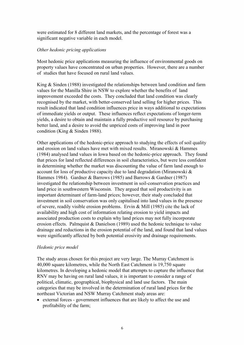
The general observations made from the Victorian and NSW surveys are summarisedin Table 1. The average area purchased was 115 hectares, and the average price paidwas $178 499, or $2732/ha. The average area of RNV on the purchased propertieswas 35 hectares, or 33% of the total property. Forty-six percent of respondents weremaking an additional purchase of land, and 45% of the properties contained a house atthe time of purchase. The average age of the purchasers was 46, and their averagelength of education was 12 years. The average household gross income was $68 417,with 40% of this being derived from on-farm income. Seventeen percent of therespondents had no on-farm income, while 20% derived their total income from on-farm production. Fifty-three percent of the respondents were members of Landcare.

Table 1Summary of general observations for Victorian and NSW surveys

Measurement Victoria New South WalesNumber of respondentsAverage area purchased (ha)Average price paid ($)Average price per hectare ($/ha)Average area of RNV (ha)Proportion of RNV (%)Additional purchase (%)House on purchased property (%)Average age of purchaser (years)Average length of Education (years)Average household gross income ($)On-farm income (%)Landcare member (%)

80115

178,4992,732

353346454612

68,4174053

44656

498,2759801422180584513

112,3597456

Of the factors listed in Q49 of the survey (in order of importance), water availability,appearance of the landscape, good view, potential income, a place to bring up a familyand the presence of RNV added most to the value of the land at the time of purchase,while weeds and pests, fire risk and adjacent pine forest detracted most from the valueof the property. It is interesting to note that aesthetic factors such as the appearance ofthe landscape and a good view were rated more highly than the perceived productivecapacity of the property. The top rating of water availability is supported by a recentsurvey of 58 properties advertised in The Land and the Stock and Land. In thedescriptions provided for these properties, factors such as access to power andtelephone, water availability, the presence or area of trees, a view, school access,topography, soil type and fencing were highlighted. Water availability was the factorreferred to most often (72% of advertisements), followed by the presence of a house(66%). The presence of trees was highlighted in 21 % of advertisements.

The influence of the clearance regulations on property values deserves examination.Thirty-four percent of Victorian properties were purchased prior to November 1989,the remainder after the introduction of the legislation. There was no significantdifference in the sale price per hectare before or after the introduction of thelegislation (Wilcoxon rank sum test z = -1.10, n = 52,28, p = 0.27). The introduction

14

of the clearance legislation had no significant influence on the purchaser’s futureintentions to clear (Pearson’s �2 = 0.05, df = 1, p = 0.82). This suggests that thelegislation may have had no influence on prices because it is perceived to be aregulation that is not strictly upheld, thus future ‘improvements’ to the purchasedproperty may still include the option to clear. Alternatively, the legislation may haveno influence on the purchase price because the purchaser may have no intentions toclear in the future.

New South Wales

Due to the lack of information on sales records within the NSW study area, surveyparticipants could not be selected in a purposive manner as they had been in Victoria.Of the 255 landholders contacted, seventy respondents declined to participate in thesurvey at the time of the initial phone call, and fifty-nine refused once they had beensent the initial information sheets. The reasons given were similar to those of theVictorian respondents, however it was felt that anxiety and suspicion regarding themore recent land clearance legislation in NSW was in large part to blame for thedisappointing response rate (49%). Of the 122 participants surveyed on a randombasis in the Murray Catchment, 44 indicated that they had made a purchase of landcontaining RNV in the last ten years. It is not possible to estimate what proportion oftotal properties sold with RNV this figure represents.

The general observations made from the Victorian and NSW surveys are summarisedin Table 1. The average area purchased was 637 ha, and the average price paid was$521, 560 or $987/ha. The average area of RNV on purchased properties was 145 ha,which is 19% of the total area purchased. Eighty-two percent of respondents weremaking an additional purchase of land, and 57% contained a house at the time ofpurchase. The average age of the purchasers was 44, and their average length ofeducation was 13 years. Average household gross income was $113,318, with 76% ofthis being derived from on-farm income. Five percent of the respondents had no on-farm income, while 30% indicated that their sole source of income was from on-farmproduction. Fifty-seven percent of the respondents were members of a Landcaregroup.

Of the factors listed in Q49 of the survey (in order of importance), potentialagricultural income, water availability, access to property already owned, appearanceof the landscape and potential capital gain were the most important factors affectingthe value of the land, while weeds and pests, fire risk and shire rates detracted mostfrom the value. In comparison to the Victorian results, factors affecting productionappear to have a higher priority than the aesthetic values in influencing propertyvalues.

15

4.2 Hedonic models

Victoria

The rural land market in the northeast Victorian catchment appears to be suitable forthe application of the hedonic technique, as it is characterised by a differentiatedproduct (rural land) being sold in a competitive market. The flow of information inthis market appears to be very good, with many real estate agents advertising withinthe region, as well as more widely. There are no large buyers or sellers in the marketwho could individually influence this market for rural land, and there are no barriersto entry apart from insufficient finance. Therefore, the assumption of purecompetition can be made for this market.

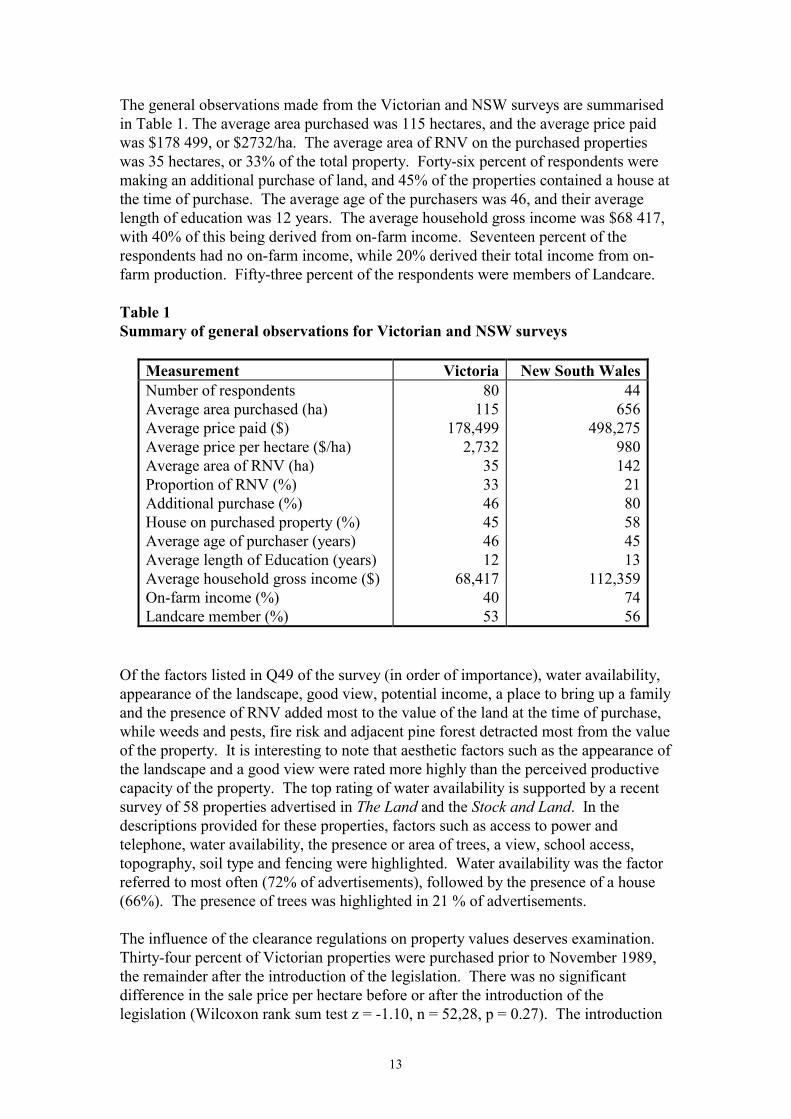
Following the discussion of functional forms in Section 3, ordinary least squaresestimates of the linear, log-linear, and log-log functional forms were undertaken basedon Equation (3), and these are presented in Table 2. Adjusted sale price1 (PRICE) wasthe dependent variable for the linear model while the natural log of (PRICE) was thedependent variable for the log-linear and log-log models. In the log-log model, thenatural log of AREA and RANK2 were taken, while the dichotomous variablesremained untransposed. A large number of the estimated coefficients had t-ratios thatwere not significant at the ten percent level, thus were omitted from the final models.

The correlation coefficients of the independent variables revealed no significantmulticollinearity between any of the variables. Given the spatial nature of the data, theexistence of heteroskedasticity in the models also needed to be tested. The SHAZAMpackage (White 1993) provides a number of tests for various forms ofheteroskedasticity. All tests for the log-log and log-linear models were insignificant,while six of the calculated statistics indicated significant heteroskedasticity in thelinear model. Therefore, a heteroskedastic consistent covariance matrix (White 1980)was employed in further analysis to correct the estimates for an unknown form ofheteroskedasticity.

The choice between the linear, log-linear, or log-log models is guided by the modifiedJ-test and Ramsey Reset test. The F-values of the Ramsey Reset test for the log-linearand log-log functional forms are all insignificant at the 5% level, but are all significantfor the linear model, indicating misspecification in the linear model. Following Coelliet al. (1991), a modified J-test2 was carried out. The t-ratios relevant to this test are

1 The PRICE variable is expressed in 1997 dollars, having been adjusted by an index of rural landvalues supplied by the Victorian Office of the Valuer-General. Total price is used as the dependentvariable as opposed to per hectare property price, as the majority of rural properties advertised for salein publications such as The Land, Stock and Land and The Weekly Times express values as totalamounts. This choice is also supported by testing for heteroskedasticity in the estimated models, whereit was found that no significant heteroskedasticity exists in the preferred model.2 The J-test is a test of non-nested hypotheses. Its calculation for the case of two models involves twosteps. Firstly each model is estimated and its predictions stored. Then each prediction is included as aregressor in the competing model . The J-test needs to be modified when the dependent variables arenot the same by suitably transforming the predictions of one model before including them as a regressorin the other. Three conclusions can be drawn from a J-test: (i) if the t-ratios of the included predictionsare either both significant or both insignificant neither model is preferred to the other; (ii) if predicitionsof model 1 in model 2 is significant and the converse insignificant, then model 1 is preferred; and (iii) if

16

predictions of model 2 in model 1 are significant and the converse insignificant, then model 2 ispreferred.

17

Table 2Hedonic price functions for the three alternative functional forms for allVictorian surveysa

Independentvariables

Lineardepvar = PRICE

Log-lineardepvar = log (PRICE)

Log-Logdepvar=log (PRICE)

AREA

HOUSE

RANK2

GEO4

BVT2

PROP50

intercept

484.43(6.43)

130390.00(6.88)

12262.00(2.97)

70014.00(3.16)

36343.00(1.86)

-48543.00(2.19)

-29321.00

0.20E-02(4.36)

0.77(6.65)

0.07(2.81)

0.23(1.73)

0.29(2.42)

-0.41(3.00)

10.72

0.22(3.65)

0.79(6.47)

0.27(2.60)

0.26(1.81)

0.29(2.31)

-0.41(2.91)

9.93

R square

R square-adj

RESET(2)

RESET(3)

RESET(4)

N

0.66

0.63

7.07

6.81

5.44

80

0.61

0.58

0.01

0.34

0.56

80

0.58

0.55

3.28

1.73

1.52

80aT-ratios are in parentheses.

18

presented in Table 3, and it can be concluded that the log-linear model is preferredover the linear and log-log model, while no difference could be discerned between thelinear model and the log-log model. On the basis of this test and the Ramsey Resettest, it is concluded that the log-linear model is superior overall.

Table 3T-ratios for the J-Test for functional form (Table 2 models)

_________________________________________________

Model into which predictions are included

Model fromwhichpredictionswere derived

linear log-linear log-log

linear

log-linear

log-log

****

2.05

2.52

-0.71

****

0.54

3.13

3.07

****

Limited Victorian Data

Using adjusted sale price (PRICE) as the dependent variable, preliminary modellingattempts using the full data set (n = 80), with proportion of RNV (PRRNV) as the keyindependent variable, did not show a significant relationship. Breaking down the dataset according to the PRRNV variable revealed that for sales of properties withPRRNV of <35% (n = 48), there was a positive relationship between price andPRRNV, while for properties with PRRNV>=35% (n = 32), there was a negativerelationship between price and PRRNV. This indicated that a non-linear relationshipexists between PRICE and PRRNV. Therefore it was decided to include bothPRRNV and PRRNV2 in the model to represent this relationship. A higher proportionof RNV on a property is more likely to have a negative influence on landholders thatdepend upon the area of land available to them for agricultural production. Furtherexamination of the data revealed that properties with >60% RNV were predominantly‘hobby’ farms with a high proportion of off-farm income. In order to have a samplethat reflected landholders with a significant level of on-farm income, these surveyresponses were excluded from further model estimations.

Linear, log-linear and log-log models were estimated based on Equation (3), and arepresented in Table 4. A large number of the estimated coefficients had t-ratios thatwere not significant at the ten percent level, thus were omitted from the final models,with the exception of PRRNV and PRRNV2, which were retained despite their lackof significance. The correlation coefficients of the independent variables revealed nosignificant multicollinearity between any of the variables. All heteroskedasticity tests

19

Table 4Hedonic price functions for the three alternative functional forms for limitedVictorian surveysa





AREA

HOUSE

GEO4

EROS

RANK2

BVT2

PRRNV

PRRNV2

intercept

521.42(6.69)

0.14E-06(6.76)

88661.00(3.51)

-61458.00(2.89)

11110.00(2.66)

56208.00(2.59)

60084.00(0.27)

-0.34E-06(0.87)

31411.00

0.22E-02(4.66)

0.76(5.91)

0.30(1.97)

-0.28(2.14)

0.05(1.98)

0.37(2.83)

0.98(0.73)

-3.57(1.52)

11.09

0.28(4.06)

0.79(5.72)

0.41(2.38)

-0.42(1.89)

0.27(2.46)

0.42(2.52)

-0.10(1.67)

0.16(0.85)

9.34

R square

R square-adj

RESET(2)

RESET(3)

RESET(4)

N

0.71

0.66

8.67

8.24

5.53

66

0.62

0.57

0.29

1.57

1.03

66

0.57

0.51

5.87

3.68

2.67


20

for the linear and log-linear models were insignificant, while three of the calculatedstatistics indicated significant heteroskedasticity in the log-log model. Therefore, aheteroskedastic consistent covariance matrix (White 1980) was employed in furtheranalysis to correct the estimates for an unknown form of heteroskedasticity. Thechoice of model is guided by the modified J-test and the Ramsey Reset test. The log-linear functional form is the only one for which all of the F-values of the RamseyReset test are insignificant at the 5% level, indicating misspecification of the linearand log-log models. The t-ratios of the modified J-test are presented in Table 5, and itcan be concluded that the log-linear model is preferred over the log-log model, whileno difference could be discerned between the linear model and the log-linear or log-log model. On the basis of this test and the Ramsey Reset test, it is concluded that thelog-linear model is superior overall.


_________________________________________________




linear

log-linear

log-log

****

2.28

2.72

-2.67

****

1.06

3.59

3.57

****

New South Wales

The Murray catchment rural land market appears to be suitable for the application ofthe hedonic technique for the same reasons given in the Victorian results section (p.14). However, it is important to note that the Murray catchment is much larger thanthe northeast Victorian catchment, with considerably more environmental variation interms of climate and landform, and would probably not be viewed as a homogenousunit by potential land purchasers. In addition, only 44 NSW survey respondentsindicated that they had made a land purchase in the past 10 years, which may not be alarge enough sample size to adequately explain variation in market values.

Ordinary least squares estimates failed to reveal any statistically significantrelationships that included RNV, with low t-values and R2 values recorded. Therefore,no models will be presented in this section.

21

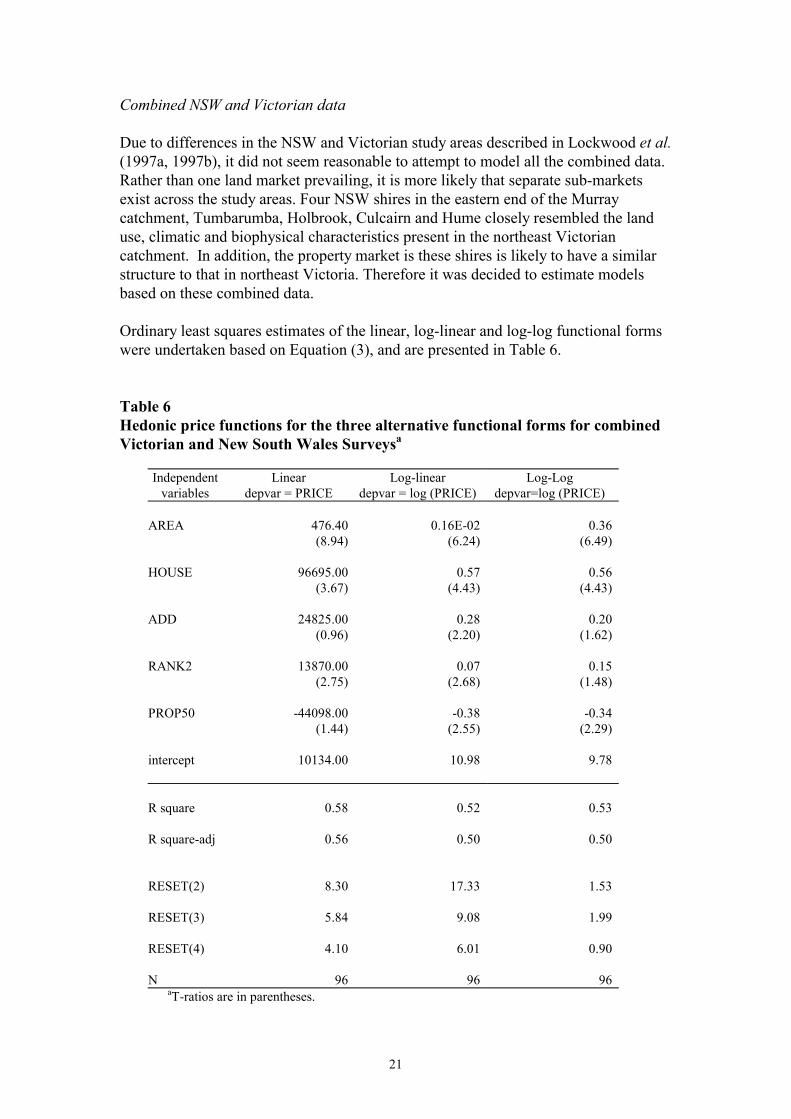
Combined NSW and Victorian data

Due to differences in the NSW and Victorian study areas described in Lockwood et al.(1997a, 1997b), it did not seem reasonable to attempt to model all the combined data.Rather than one land market prevailing, it is more likely that separate sub-marketsexist across the study areas. Four NSW shires in the eastern end of the Murraycatchment, Tumbarumba, Holbrook, Culcairn and Hume closely resembled the landuse, climatic and biophysical characteristics present in the northeast Victoriancatchment. In addition, the property market is these shires is likely to have a similarstructure to that in northeast Victoria. Therefore it was decided to estimate modelsbased on these combined data.

Ordinary least squares estimates of the linear, log-linear and log-log functional formswere undertaken based on Equation (3), and are presented in Table 6.

Table 6Hedonic price functions for the three alternative functional forms for combinedVictorian and New South Wales Surveysa





AREA

HOUSE

ADD

RANK2

PROP50

intercept

476.40(8.94)

96695.00(3.67)

24825.00(0.96)

13870.00(2.75)

-44098.00(1.44)

10134.00

0.16E-02(6.24)

0.57(4.43)

0.28(2.20)

0.07(2.68)

-0.38(2.55)

10.98

0.36(6.49)

0.56(4.43)

0.20(1.62)

0.15(1.48)

-0.34(2.29)

9.78

R square

R square-adj

RESET(2)

RESET(3)

RESET(4)

N

0.58

0.56

8.30

5.84

4.10

96

0.52

0.50

17.33

9.08

6.01

96

0.53

0.50

1.53

1.99

0.90


22

Adjusted sale price (PRICE) was the dependent variable for the log-linear and log-logmodels. In the log-log model, the natural log of AREA and RANK2 were taken,while the dichotomous variables remained untransposed. A large number of theestimated coefficients had t-ratios that were not significant at the ten percent level,thus were omitted from the final models. The correlation coefficients of theindependent variables revealed no significant multicollinearity between any of thevariables. Tests indicated that no significant heteroskedasticity existed in the log-linear and log-log models, while all of the calculated statistics indicated significantheteroskedasticity in the linear model. Once again, a heteroskedastic consistentcovariance matrix was employed in further analysis to correct the estimates for anunknown form of heteroskedasticity. The F values of the Ramsey Reset test for thelog-log functional form are all insignificant at the 5% level, and are all significant forthe log-linear and linear model, indicating misspecification in the log-linear and linearmodels. The t-ratios of the modified J-test are presented in Table 7, and it can beconcluded that the linear model is preferred over the log-log model, while the log-linear model is preferred over the log-log model. No difference could be discernedbetween the linear and log-linear models. On the basis the Ramsey Reset test and theheteroskedasticity tests, the log-log model is preferred, while on the basis of themodified J-test either the linear or log-linear model is preferred. It was concludedearlier in this report that the use of a non-linear functional form was more appropriatefor this type of analysis, while the presence of heteroskedasticity will lead to estimatedcoefficients that are inefficient. Therefore, the log-log model will be used for furtherinterpretation.


_________________________________________________




linear

log-linear

log-log

****

-2.83

1.43

4.47

****

1.32

2.88

2.72

****

23

4.3 Interpretation of the preferred models

In the preferred log-linear model in Table 2, all coefficients have the expected sign.The regression estimate fits the data reasonably well, with 61% of variation in thedependent variable being explained. The remaining variation can most likely beexplained by the omission of important variables, as well as the use of proxy variablesand random errors. The size of the property (AREA) and the presence of a house(HOUSE) have a strong positive influence on property value. The presence ofsedimentary parent material on the property (GEO4), and fences with good conditionand placement (RANK2), also have a positive influence on property value. Thepresence of dry foothill forest (BVT2) has a positive influence on property value,while the existence of RNV at a proportion greater than 50% (PROP50) has a negativeinfluence.

The coefficients of a log-linear equation represent the average percentage change invalue for a unit change in a characteristic (marginal price), therefore a literalinterpretation of this coefficient suggests that the presence of dry foothill forest wouldraise the value of the average property by 29%, or $51,764. However, this resultcannot be interpreted in terms of the amount of RNV on the property, only itspresence or absence. The BVT2 (Dry Foothills forest) variable was examined furtherto see if it was acting as a proxy for any other measurements not included in themodel. Correlation coefficients between BVT2 and all other variables used inpreliminary modelling attempts revealed significant relationships between BVT2 andLAND4 (r = 0.38, p < 0.001), BVT2 and BVT3 (r = -0.40, p < 0.001), and BVT2 andBVT6 (r = -0.59, p < 0.001). The relationship between BVT2 and LAND4 is areflection of the occurrence of this vegetation type in steeper areas. A negativerelationship exists between BVT2 and BVT3 and 4, indicating that these vegetationtypes occur in areas where BVT2 is not present. Therefore, it can be concluded thatBVT2 is not acting as a proxy for other variables and appears to be a truerepresentation of the presence of this particular vegetation type.

The continuous RNV variables RNVHA and PRRNV did not enter the model assignificant variables. The introduction of PROP measurements enabled thecategorisation of properties according to whether they exceeded a particularproportion of RNV, represented as a dichotomous (0/1) variable. Only PROP50entered the model as a significant coefficient, suggesting that for properties purchasedwith a proportion of RNV exceeding 50%, the average property value would bedecreased by 41% or $73,184. This result suggests that any benefits associated withthe presence of BVT2 will be outweighed by the costs by the greatest amount whenthe proportion of RNV exceeds half of the total property area. Twenty-five percent ofthe survey respondents had more than 50% RNV.

In the preferred log-linear model in Table 4, all coefficients are of the expected sign.The regression estimate fits the data reasonably well, with 62% of variation in thedependent variable being explained. The size of the property (AREA) and thepresence of a house (HOUSE) have a strong positive influence on property value. Thepresence of sedimentary parent material on the property (GEO4), and fences withgood condition and placement (RANK2), also have a positive influence on propertyvalue. The presence of soil erosion on the property (EROS) has a significant negative

24

impact upon property value. The presence of dry foothill forest (BVT2) has a positiveinfluence on property value, while the proportion of RNV (PRRNV and PRRNV2)had the expected signs, but were not significant at the ten percent level.

The signs on the PRRNV and PRRNV2 coefficients in Table 4 are expected, in thatthey reflect the curvilinear relationship that appeared evident upon initial modellingattempts described earlier in this section. However, the t-ratios on the estimatedcoefficients are less than 1.65. Therefore, the implicit marginal value of PRRNV isnot significantly different from zero at the ten percent level

It is useful to compare the results from the preferred models in Table 2 and 4, giventhat the results from Table 4 exclude the survey responses from Victorian landholdersidentified as hobby farmers. The independent variable EROS appears in the estimatedmodels in Table 4, indicating that these landholders may be more aware of thepotential of erosion to diminish agricultural productivity. The BVT2 variable appearsin both models, although it is interesting to note that the coefficient is larger for thelimited survey model, indicating a larger benefit from the presence of this particularbroad vegetation type for this group of landholders. An explanation for this result isthat the larger sample containing hobby farmers may be reflecting a preference forland that contains vegetation of higher conservation value.

The possibility that confounding effects may exist between the amount of RNV, thearea of land purchased and the area of cleared land needs to be tested. Correlationcoefficients estimated between AREA and PROP50, and AREA and PRRNVindicated that such confounding effects were not present in the model. The preferredmodel from Table 2 was re-estimated using CLEAR instead of AREA. The R2 valueswere lower (0.58, 0.55), and the variable GEO4 was no longer significant. Thepreferred model from Table 4 was re-estimated using CLEAR instead of AREA, andRNVHA instead of PRRNV. The R2 values were lower (0.56, 0.53), and the GEO4and EROS variables were no longer significant. In addition, there was significantcorrelation between CLEAR and RNVHA (r = 0.43, p < 0.001). On this basis, it wasdecided to retain the models reported in Table 2 and Table 4.

The preferred log-linear model estimated from the combined Victorian and NSW data(Table 6) contains five significant independent variables of the expected sign. Fifty-three percent of variation in the dependent variable is explained by the regression. Thesize of the property (AREA) and the presence of a house (HOUSE) have a strongpositive influence on property value. The purchase of property in addition to landalready owned (ADD), and fences with good condition and placement (RANK2), alsohave a positive influence on property value. The existence of RNV at a proportiongreater than 50% (PROP50) has a negative influence. In comparison to the preferredVictorian model in Table 2, this model explains less of the variation in the dependentvariable, the geology variable (GEO4) has dropped out, replaced by the explanatoryvariable (ADD), which reflects the higher proportion of NSW landholders who weremaking an additional purchase of land. The remnant vegetation variable PROP50 hasa slightly lower estimated coefficient, but is still highly significant, suggesting that forproperties purchased with a proportion of RNV exceeding 50%, the average propertyvalue would be decreased by 38% or $79,743 (average PRICE for the combinedsurveys was $209,851).

25

5. Discussion and conclusions

The decision to purchase land is a very complex one, with a range of factors needingto be taken into consideration. Attempts were made to measure and include as manyof these factors as possible in preliminary hedonic models. However, it becameevident that only a small proportion of these factors were having a significantinfluence on the sale value of the property. These factors included consumption,production and vegetation characteristics of the property. It also became evident thatthe small sample size in NSW was not going to be sufficient to develop a reasonablemodel to reflect the market in the Murray catchment.

The non-agricultural benefits of RNV

As part of the wider on-farm survey (see Miles et al. 1998), respondents were asked toindicate the benefits they believed their RNV provided in terms of a number ofenvironmental services. Of the predetermined benefits listed in the survey, aestheticswas regarded by 89% of Victorian respondents and 93% of NSW respondents asproviding a benefit, but a quantitative measurement of this type of on-farm benefitwas not attempted. The attitude of respondents was that the presence of treesimproved the attractiveness of the landscape, that the look of bare treeless paddocksand hills was highly undesirable, and in some cases that the trees had a spiritual,therapeutic effect. Most of the aesthetic benefits were expressed in terms of visualamenity. A selection of the comments are listed in Appendix II. It could be that thebenefit value of $51,764 calculated from the BVT2 coefficient may be encompassingsome of the on-farm aesthetic values associated with the presence of RNV on aproperty, or acting as a ‘proxy’ for aesthetics.

The dry foothill forest measurement (BVT2) represented in the preferred models is themost predominant RNV type on private land in the northeast catchment, making up76,480 out of a total of 115,945 hectares of RNV. This BVT is generally restricted tosteeper foothills on low fertility soil types. The presence of this variable in the modelas a positive and significant coefficient suggests that landholders may be happy toaccept the presence of this type of RNV on parts of their property not seen as highlyproductive and readily accessible, and therefore is not perceived as directly competingfor land that supports their major agricultural enterprises. Respondents to the survey(Q49.11) indicated that the presence of RNV on the property was an important factorin their decision to purchase. These sentiments seem to be reflected in the hedonicmodel by BVT2, but are countered once the RNV exceeds a certain proportion.

The provision of aesthetic values associated with RNV are generally perceived as apublic good that benefits the wider community. Fry & Sarlöv-Herlin (1997) suggestthat farmers and non-farmers see the same landscape image, but will perceive itdifferently and with different objectives in mind. What is rarely considered is thatindividual landholders may also value RNV in terms of the visual amenity benefits itprovides. The exchange of property in the market allows a formal expression bylandholders of this benefit. The results of this hedonic analysis seem to suggest thatthere may be an on-farm willingness to pay for the amenity benefits provided by

26

RNV, however it is difficult to know how much of the benefit value apparentlyassociated with BVT2 can be attributed to this factor.

The hedonic pricing model has proved to be a useful method for highlighting thepositive and negative aspects of RNV that have influenced sale prices for propertiespurchased in the last ten years in northeast Victoria. The model appears to bemeasuring some non-agricultural benefits that landholders attribute to the presence ofRNV on their property, while also reflecting that there are also measurable negativeimpacts on sale values associated with having ‘too much’ RNV. Below this thresholdhowever, the area of RNV appears to have little influence on property price.

Use of the results in the wider benefit cost analysis

In a perfect market with full information, property prices should reflect, amongst otherthings, all costs and benefits associated with RNV. Economic benefits of RNVinclude increased stock production, increased agricultural production arising frommitigation of land degradation, increased crop production from shelter and shadeeffects, and timber for firewood and fencing. Any economic value arising fromscenery and nature conservation benefits of RNV would also be reflected in propertyprice. Costs of RNV include pest plant and animal control, fire management andfencing. In the landholder surveys, 53% of participants in northeast Victoria and 82%in the Murray catchment currently enjoy a net benefit from their RNV (Miles et al.1998). A perfect property market would reflect this net benefit. It would therefore bedouble counting to include in a benefit cost analysis both a property price componentand a direct assessment of RNV costs and benefits. With perfect information, aproperty market and direct surveys should produce the same estimate of net economicvalue. However, based on the results of this hedonic analysis, the property market isnot at present a good measure of the economic value of RNV. Presumably this isprimarily due to the lack of information and awareness on the part of both buyers andsellers. The more accurate direct survey data will therefore be used in benefit costsanalyses to be conducted as part of the wider project.

27

6. References

Anderson, L.M., Cordell, H.K. (1988) Influence of trees on residential propertyvalues in Athens, Georgia (USA): a survey based on actual sales prices. Landscapeand Urban Planning 15:153-164.

Barrows, R., Gardner, K. (1987) Do land markets account for soil conservationinvestment? Journal of Soil and Water Conservation 42(4): 232-236.

Butler, R.V. (1982) The specification of housing indexes for urban housing. LandEconomics 58: 96-108.

Clifton, I.D., Spurlock, S.B. (1983) Analysis of variations in farm real estate pricesover homogenous market areas in the southeast. Southern Journal of AgriculturalEconomics 15:89-96.

Coelli, T., Lloyd-Smith, J., Morrison, D., Thomas, J. (1991) Hedonic pricing for acost benefit analysis of a public water supply scheme. Australian Journal ofAgricultural Economics 35(1): 1-20.

Cropper, M.L., Deck, L.B., McConnell, K.E. (1988) On the choice of functional formfor hedonic price functions. The Review of Economics and Statistics 70: 668-675.

Ervin, D.E., Mill, J.W. (1985) Agricultural land markets and soil erosion: policyrelevance and conceptual issues. American Journal of Agricultural Economics 67(3):938-932.

Freeeman, A.M. (1979) Hedonic prices, property values and measuringenvironmental benefits: a survey of the issues. Scandinavian Journal of Economics81: 154-173.

Fry, G., Sarlöv-Herlin, I. (1997) The ecological and amenity functions of woodlandedges in the agricultural landscape; a basis for design and management. Landscapeand Urban Planning 37: 45-55.

Gardner, K., Barrows, R. (1985) The impact of soil conservation investments on landprices. American Journal of Agricultural Economics 67(3): 943-947.

Garrod, G., Willis, K. (1992a) Valuing goods’ characteristics: an application of thehedonic price method to environmental attributes. Journal of EnvironmentalManagement 34: 59-76.

Garrod, G., Willis, K. (1992b) The amenity value of woodland in Great Britain: acomparison of economic estimates. Environmental and Resource Economics 2: 415-434.

Garrod, G., Willis, K. (1992c) The environmental economic impact of woodland: atwo-stage hedonic price model of the amenity value of forestry in Britain. AppliedEconomics 24: 715-728.

28

Geoghegan, J., Wainger, L.A., Bockstael, N.E. (1997) Spatial landscape indices in ahedonic framework: an ecological economics analysis using GIS. EcologicalEconomics 23(3):251-264.

Graves, P., Murdoch, D.C., Thayer, M.A., Waldman, D. (1988) The robustness ofhedonic price estimation: urban air quality. Land Economics 64: 220-233.

Griffiths, W.E., Hill, R.C., Judge, G.G. (1993) Learning and practicingeconometrics. John Wiley and Sons, New York.

Halstead, J.M., Bouvier, R.A., Hansen, B.E. (1997) On the issue of functional formchoice in hedonic price functions: further evidence. Environmental Management21(5): 759-765.

Harris, A.H. (1981) Hedonic technique and valuation of environmental quality, inSmith, V. Kerry (ed.) Advances in Applied Microeconomics. JAI Press, Greenwich,pp 31-49.

King, D.A., Sinden, J.A. (1988) Influence of soil conservation on farm land values.Land Economics 64(3): 242-255.

Linneman, P. (1980) Some empirical results on the nature of the hedonic pricefunction for the urban housing market. Journal of Urban Economics 8: 47-68.

Lockwood, M., Buckley, E., Glazebrook, H. (1997) Remnant vegetation on privateproperty in northeast Victoria. Johnstone Centre Report No. 94. Johnstone Centre,Albury.

Lockwood, M., Buckley, E., Glazebrook, H. (1997) Remnant Vegetation on PrivateProperty in the Southern Riverina, NSW. Johnstone Centre Report No. 95.Johnstone Centre, Albury.

Lockwood, M., Carberry, D. (1998) Stated preference surveys of remnant nativevegetation conservation. Johnstone Centre Report No. 104. Johnstone Centre,Albury.

MacKinnon, J.G. (1983) Model specification tests among non-nested alternatives.Econometric Reviews 2:85-110.

Marano, W.A.J. (1998) Factors influencing the market value of remnant nativevegetation in South Australia, 1982-1994. Final report to EnvironmentAustralia/Land and Water Resources Research and Development Corporation.University of South Australia, Adelaide (in prep.).

Miles, C.A. (1998) An assessment of the on-farm economic values associated withremnant vegetation in northeast Victoria. BAppSci (Hons) thesis, Charles SturtUniversity, Albury.

29

Miles, C.A., Lockwood, M., Walpole, S.C. (1998) Assessment of the on-farmeconomic values of remnant native vegetation. Johnstone Centre Report No. 107.Johnstone Centre, Albury.

Miles, C.A., Lockwood, M., Walpole, S.C. (1998) Incentive policies for remnantnative vegetation. Johnstone Centre Report No. 108. Johnstone Centre, Albury.

Milton, J.W., Gressel, J., Mulkey, D. (1984) Hedonic amenity valuation andfunctional form specification. Land Economics 60(4): 378-387.

Miranowski, J.A., Hammes, B.D. (1984) Implicit prices of soil characteristics forfarmland in Iowa. American Journal of Agricultural Economics 66(5): 745-749.

Morales, D.J. (1980) The contribution of trees to residential property value. Journalof Arboriculture 6(11): 305-308.

Palmquist, R.B. (1991) Hedonic Methods, in Braden, J.B., Kolstad, C.D. (eds)Measuring the demand for environmental quality. Elsevier Science, Holland, pp. 77-120.

Palmquist, R.B., Danielson, L.E. (1989) A hedonic study of the effects of erosioncontrol and drainage on farmland values. American Journal of AgriculturalEconomics 71(1): 55-62.

Powe, N.A., Garrod, G.D., Brunsdon, C.F., Willis, K.G. (1997) Using a geographicinformation system to estimate an hedonic price model of the benefits of woodlandaccess. Forestry 70(2): 139-149.

Ramsey, J.B. (1969) Tests for specification error in classical least squares regressionanalysis. Journal of the Royal Statistical Society 31: 250-271.

Reynolds, I.K. (1978) The relationship of land values to site characteristics—someimplications for scenic quality management. Journal of Environmental Management6: 99-106.

Rosen, S. (1974) Hedonic prices and implicit markets: product differentiation in purecompetition. Journal of Political Economy 2: 34-55.

Streeting, M. (1990) A survey of the hedonic pricing technique. ResourceAssessment Commission Research Paper No. 1, Resource Assessment Commission.AGPS, Canberra.

Tyrväinen, L. (1997) The amenity value of the urban forest: an application of thehedonic pricing method. Landscape and Urban Planning 37:211-222.

Valuer General’s Office (1996) Real Estate Values 1996. Valuer General’s Office,Sydney.

30

White, H. (1980) A heteroskedasticity-consistent covariance matrix and a direct testfor heteroskedasticity. Econometrica 48: 817-838.

White, K.J. (1993) SHAZAM user’s reference manual Version 7.0. McGraw-Hill,New York.

Williams, C.H., Rolfe, J., Longworth, J.W. (1993) Does muscle matter? An economicevaluation of live cattle characteristics. Review of Marketing and AgriculturalEconomics 61: 169-189.

31

Appendix I The farm survey instrument

32

NSW DATA ENTRY FORM (face to face and phone interviews)

As discussed on the phone, this survey involves determining what the benefits and costs are toyou for conserving remnant native vegetation. The information that we sent out to you will beuseful to have on hand while we go through these questions. Your participation in the survey iscompletely voluntary and the answers will be kept confidential, please read and sign the consentform if you haven’t already done so. This survey will take about one hour to complete.

PART A General background information

1. What is the size of your property? ___________ (ha/acres)

2. What are the main farming enterprise/s undertaken on this property? (respondent to describe) 1 � Grazing of sheep for mutton 2 � Grazing of sheep for wool 3 � Grazing of cattle (beef) 4 � Farm forestry 5 � Dairying 6 � Cropping 7 � Horticulture (please specify) ________________ 8 � Irrigation 9 � Hobby farm10 � Other (please specify) ________________

3. How much remnant vegetation in total is present on your property? ____________(ha/acres)

Definition of RNV: Remaining patches or clumps of native trees and shrubs greater than 1hectare (2.5 acres) in size.

4. How many different patches of remnant vegetation (greater than 1 ha) are present on your property?

_______________ patches

5. How big is the largest patch of remnant vegetation on your property? __________(ha/acres)

6. How would you rate the quality/condition of your remnant(s)?

The three quality ratings are degraded, modified and intact:

Degraded: Regular grazing, no tree hollows, no fallen timber, no overstorey regeneration, muchtree dieback present, no understorey shrubs.

Modified: Lightly grazed, a few tree hollows present, a little fallen timber present, a littleoverstorey regeneration present, some tree dieback present, some understorey shrubs.

Intact: Not grazed/rarely grazed, some/many tree hollows present, some/a lot of fallen timberpresent, some/a lot of overstorey regeneration present, none/little tree dieback present,some/much understorey shrubs.

Which of these best describes your remnant(s)?

1 � Degraded 2 � Modified 3 � Intact

7. Are you aware of any interesting or unusual plants and animals on your property?0 � No 1 � Yes 99 � Don’t know

33

If yes, please describe___________________________________________________

* * * *

PART B

This next section asks information about the on-farm costs and benefits of conserving remnantnative vegetation

8. Are any of your areas of remnant vegetation fenced off? 0 � No 1 � Yes

a. If yes, 1 � metres of fencing erected______________(m)2 � area fenced off______________________(ha/acres)

If erected 3 � cost of materials_____________________($)by yourself, 4 � personal labour______________________(hours)

5 � contract labour______________________($)

9. Are your remnant(s) used for grazing? 0 � No 1 � Yes

a. If yes, 1 � number and type of sheep__________________(number/year/wool or meat)2 � time spent in remnant(s) _____________(weeks/year)

b. If yes, 1 � number and type of cattle_____________(number/year/vealers/steers or dairy)2 � time spent in remnant(s) _____________(weeks/year)

10. Please describe how your remnant(s) are used (apart from grazing) as part of your current farmingpractices

1 � Stock shelter and shade2 � Timber extraction3 � Household firewood extraction4 � Commercial firewood extraction5 � Fence posts6 � Honey production7 � Seed collection8 � Other____________________(please specify)

11. If your remnant(s) are not used as part of your farming practices, are they used in any other ways?(eg. recreation, farm stay or any others that you can think of) (read options)

__________________________________________________________________________________12. Imagine the hypothetical situation where your remnant/s were cleared and sold. Which of thefollowing benefits would be lost as a result of not having the remnant/s on your farm? For those whichyou consider to be beneficial, please comment (eg. quantify these in terms of benefits per year, ifpossible, although we realise that this may be difficult). Please refer to Table 1 from theinformation we sent you. Tick for Yes X for No N/A for not applicable

34

Table 1 Possible benefits of RNV1 � Increased stock production due to shelter and shade (note: benefits include the ongoing and

the one-off benefits, eg. protection from storm)Benefit per year (eg. increased stocking rates, reduced lambing losses etc.)______________________________________________________________________________________________________________________________________________________

2 � Increased crop production due to shelterBenefit per year (eg. tonnes of grain)______________________________________________________________________________________________________________________________________________________

3 � Increased agricultural production due to land degradation controlBenefit per year (eg. drop in water table, decreased erosion, salinity)______________________________________________________________________________________________________________________________________________________

4 � Timber for firewood and fencingBenefit per year (eg. tonnes of wood extracted, number of posts extracted)______________________________________________________________________________________________________________________________________________________

5 � Cleaner waterBenefit (eg. decreased maintenance costs on pumps etc.)______________________________________________________________________________________________________________________________________________________

6 � Habitat for animals which help control pestsBenefit (eg. presence of ibis or other birds which eat pest insects?)______________________________________________________________________________________________________________________________________________________

7 � Nutrient cycling / soil formation___________________________________________________________________________

8 � RecreationBenefit (eg. number of visits per year made by yourself, number of visits per year made by family/friends, where they travelled from)______________________________________________________________________________________________________________________________________________________

9 � AestheticsBenefit (please describe)__________________________________________________________________________________________________________________________________

10 � OtherBenefit (please describe)__________________________________________________________________________________________________________________________________

11 � No benefits

35

13 a. Is there any chance that you would clear your RNV in the next 10 years? 0 � No 1 � Yes

13b. If yes, how much? ______________ha/acres

13c. If yes, how likely (scale from 1-5) is it that you would want to clear the RNV for the followinguses in the next ten years? Please refer to Table 2 from the information we sent you.

Table 2: Are you likely to clear remnant vegetation for the following uses?

LAND USE AFTER CLEARING very unlikely very likely13c1 Pine plantation 1 2 3 4 513c2 Native hardwood plantation 1 2 3 4 513c3 Pasture 1 2 3 4 513c4 Grape vines 1 2 3 4 513c5 Cropping (please specify type) 1 2 3 4 513c6 Rice 1 2 3 4 513c7 Other (please specify) 1 2 3 4 5

14. a. Have any areas of RNV been cleared on your property during the past ten years? 0 � No 1 � Yes

b. If yes what area was cleared____________(ha/acres)

15. If you have cleared, how is this land being used? (respondent to describe)1 � Pine plantation2 � Native hardwood plantation3 � Pasture4 � Grape vines5 � Cropping (please specify type)__________________________6 � Rice7 � Other (please specify)_________________________________

16. What direct costs are involved with the ongoing management of the remnant/s? (read options)For the following options, could you estimate how much you spend per year.� no costs

Management Expenditure($/year)

Personal labour(hours/year)

Contract labour($/year)

1 Fencinga b c

2 Weed controla b c

3 Pest controla b c

4 Other (eg. fuel reduction burning,removal of sticks from forest floor,erosion control in remnants) a b c

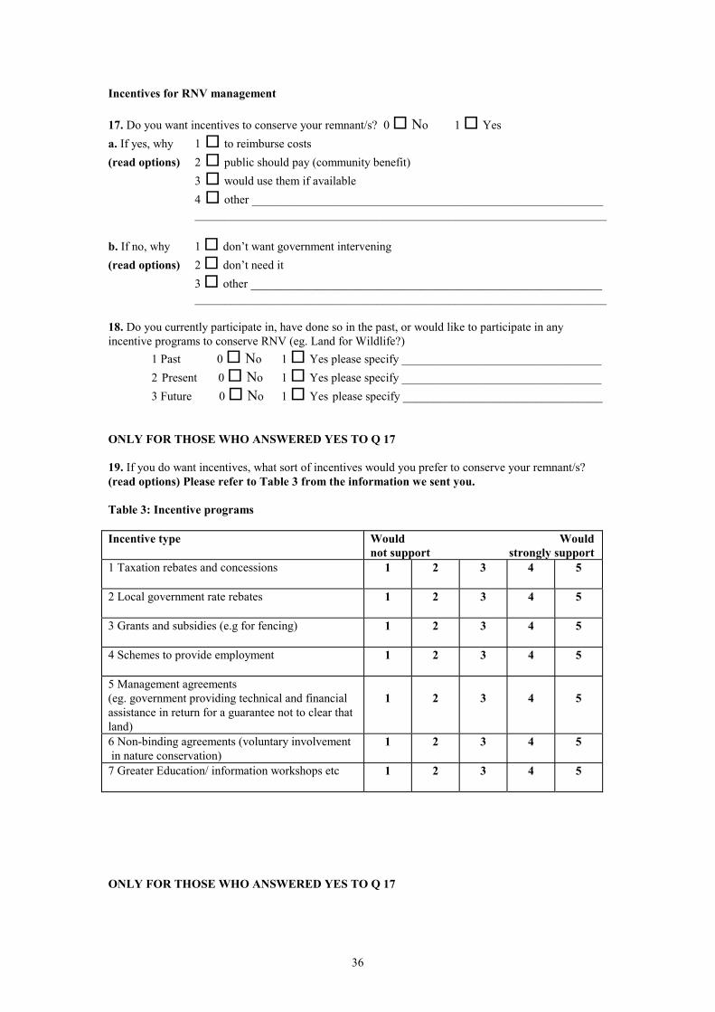
36

Incentives for RNV management

17. Do you want incentives to conserve your remnant/s? 0 � No 1 � Yesa. If yes, why 1 � to reimburse costs(read options) 2 � public should pay (community benefit)

3 � would use them if available4 � other ______________________________________________________________________________________________________________________________

b. If no, why 1 � don’t want government intervening(read options) 2 � don’t need it

3 � other ______________________________________________________________________________________________________________________________

18. Do you currently participate in, have done so in the past, or would like to participate in anyincentive programs to conserve RNV (eg. Land for Wildlife?)

1 Past 0 � No 1 � Yes please specify _________________________________2 Present 0 � No 1 � Yes please specify _________________________________3 Future 0 � No 1 � Yes please specify _________________________________

ONLY FOR THOSE WHO ANSWERED YES TO Q 17

19. If you do want incentives, what sort of incentives would you prefer to conserve your remnant/s?(read options) Please refer to Table 3 from the information we sent you.

Table 3: Incentive programs

Incentive type Would Wouldnot support strongly support

1 Taxation rebates and concessions 1 2 3 4 5

2 Local government rate rebates 1 2 3 4 5

3 Grants and subsidies (e.g for fencing) 1 2 3 4 5

4 Schemes to provide employment 1 2 3 4 5

5 Management agreements(eg. government providing technical and financialassistance in return for a guarantee not to clear thatland)

1 2 3 4 5

6 Non-binding agreements (voluntary involvement in nature conservation)

1 2 3 4 5

7 Greater Education/ information workshops etc 1 2 3 4 5


37

20. Can you suggest any other incentives which would be desirable for the management of yourremnant/s?___________________________________________________________________________________________________________________________________________________________


21. If your preferred choice of incentives and support for management were provided, would you beprepared to (read options one at a time):

1 Fence off remnants ( for conservation purposes only) 0 � No 1 � Yes 99 � Don’t know

2 Fence off remnants ( grazing permitted ) 0 � No 1 � Yes 99 � Don’t know

3 Cease clearing remnants 0 � No 1 � Yes 99 � Don’t know

4 Establish and implement a vegetation management

plan 0 � No 1 � Yes 99 � Don’t know

5 Attend information workshops regarding the management of remnant native vegetation 0 � No 1 � Yes 99 � Don’t know

38

INFORMATION ABOUT YOU AND YOUR HOUSEHOLD (O P T I O N A L)

This next section will focus on information about you and your household, keeping in mind that allquestions are optional and confidential. This information is important for us to determine whether wehave obtained a representative sample from a range of people in our study area.

22. What is your age? ___________(years)

23. What is the highest level of education you have obtained or are obtaining? (respondent todescribe)

0 � Never went to school6 � Completed primary only6+ no. � Secondary (specify year/form reached)__________13 � Completed short course(s) after secondary14 � Diploma or certificate16 � Tertiary degree? � Other (please specify)

24. To the best of your knowledge what is the household gross income (before taxes) you earned lastfinancial year? This is both on-farm and off-farm income. *exact amount better than range, if possible

Under $5 000 � 2500 $37 501 - $45 000 � 41250.5

$5 001- $12 000 � 5800.5 $45 001 - $60 000 � 52500.5

$12 001 - $18 000� 15000.5 $60 001 - $ 100 000 � 80000

$18 001 - $24 000� 21000.5 more than $100 000 � 125000

$24 001 - $30 000� 27000.5 Don’t know �

$30 001 - $37 500� 33750.5 Exact amount __________

25. What proportion of the above income (not profit) is derived from on-farmproduction?_______________(%)

26. How long have you been farming? a. on this property _________ yearsb. lifetime _________ years

27. Are you a member of any of the following organisations/voluntary groups? (read options)1 � Landcare2 � NSW Farmers Federation3 � Rural Bush Fire Brigade4 � Other (please specify)__________________________

39

28. What are your intentions for the future management of your property? (prompt if needed)1 � Maintain current management2 � Diversify farming enterprise/s3 � Sell property4 � Subdivide5 � Hand down to next generation6 � Improve management (please specify) ______________________________________7 � Other (please specify)__________________________

Further feedback

29a. Your input to our research has been very valuable. Would you be interested in continuing yourinvolvement in the project, through participation in a local workshop or discussion group regardingincentives for remnant native vegetation conservation? 0 � No 1 � Yes

29b. Would you be interested in obtaining a summary of the survey results? 0 � No 1 � Yes

40

PART C Land values and RNV

This section relates to any land purchases with remnants you have made in the past ten years.This section asks general information about the purchase and the property. This will help us todevelop a profile of the buyer and seller, and the reasons behind the purchase decision.Questions about remnants refer only to those on this purchased land.

30. Have you purchased a block of land greater than 2 ha in the past 10 years? 0 � No 1 � Yes

31. What was the area of the land purchased?_______________(ha/acres)

32. At the time of purchase, what area of the land had remnant nativevegetation?____________(ha/acres)

33. What would you consider the natural condition of the remnant/s to have been in when youpurchased the land? Describe if this is different to Q7, refer to definitions.

1 � Degraded 2 � Modified 3 � Intact 99 � Don’t know

34. Were there other potential purchasers for the land that you bought?

0 � No 1 � Yes How many others (if known)?___________ 99 � Don’t know

35. Was the seller a willing seller, or was he/she forced to sell?

1 � Willing seller? 2 � Forced to sell? 99 � Don’t know

36. Was the seller over or under 50?

1 � Under 50 2 � Over 50 99 � Don’t know

37. Was there an immediate family member of the seller who could have taken over the property?

0 � No 1 � Yes 99 � Don’t know

38. At the time of purchase, did you think the land was (read options):

1 � Unproductive 2 � Productive 3 � Highly productive 99 � Don’t know

39. At the time of purchase, did you think soil erosion levels were (read options):

1 � Low (not present) 2 � Moderate (some areas affected) 3 � High (large areas affected)99 � Don’t know

40. At the time of purchase, did you think salinity levels were (read options):

41


41. At the time of purchase, did you think soil acidity levels were (read options):


42. Was there a house on the land when you purchased it? 0 � No 1 � Yes

43. If yes, 1 Age___________(years)2 Size___________(squares)3 Number of bedrooms____________4 Number of bathrooms___________5 Gararge____________

44. Is this house now your permanent place of residence? 0 � No 1 � Yes

45. Were there any other buildings on the land when you purchased it? 0 � No 1 � YesIf yes, please specify____________________________________________________________

46. Was the land an addition to another of your properties? 0 � No 1 � YesIf so, what was the distance of the land from the home property?______________(km)

47. What was the distance of the land purchased from a bitumen road?____________(km)

48. If the area of land purchased makes up only part of the whole farm area, what was the gross incomespecifically from the purchased land during 1996/97 (ie. if different from Part B)?

_________________________________________________________________________________

42

49. Many things affect the value of land. Which of the following factors added or detracted to thevalue of the land, at the time of purchase? Please refer to Table 4 from the information we sent you.

Table 4: Factors adding or detracting Detracted most Didn’t affect Added mostto land value from the value the value to the value

1 Distance to nearest town...................................-5 -4 -3 -2 -1 0 1 2 3 4 5

2 Condition and nature of farm buildings........... -5 -4 -3 -2 -1 0 1 2 3 4 5

3 Potential agricultural income........................... -5 -4 -3 -2 -1 0 1 2 3 4 5

4 Condition and placement of fences.................. -5 -4 -3 -2 -1 0 1 2 3 4 5

5 Condition of dams etc...................................... -5 -4 -3 -2 -1 0 1 2 3 4 5

6 Condition or nature of house (if any)............... -5 -4 -3 -2 -1 0 1 2 3 4 5

7 River frontage.................................................. -5 -4 -3 -2 -1 0 1 2 3 4 5

8 Water availability............................................. -5 -4 -3 -2 -1 0 1 2 3 4 5

9 Appearance of paddocks.................................. -5 -4 -3 -2 -1 0 1 2 3 4 5

10 Appearance of landscape................................ -5 -4 -3 -2 -1 0 1 2 3 4 5

11 Presence of remnant native vegetation........... -5 -4 -3 -2 -1 0 1 2 3 4 5

12 Condition of remnant native vegetation......... -5 -4 -3 -2 -1 0 1 2 3 4 5

13 Presence of remnant native vegetation on adjoining properties.........................................-5 -4 -3 -2 -1 0 1 2 3 4 5

14 Presence of adjoining pine forest .................. -5 -4 -3 -2 -1 0 1 2 3 4 5

15 Presence of adjoining public land................... -5 -4 -3 -2 -1 0 1 2 3 4 5

16 Existence of weeds and pests.......................... -5 -4 -3 -2 -1 0 1 2 3 4 5

17 Fire risk........................................................... -5 -4 -3 -2 -1 0 1 2 3 4 5

18 Presence of conservation covenant.................-5 -4 -3 -2 -1 0 1 2 3 4 5

19 Potential to clear more land ............................-5 -4 -3 -2 -1 0 1 2 3 4 5

20 Potential capital gain....................................... -5 -4 -3 -2 -1 0 1 2 3 4 5

21 Shire rates........................................................ -5 -4 -3 -2 -1 0 1 2 3 4 5

22 Access to power and telephone....................... -5 -4 -3 -2 -1 0 1 2 3 4 5

23 Access to property already owned.................. -5 -4 -3 -2 -1 0 1 2 3 4 5

24 A place to bring up a family............................ -5 -4 -3 -2 -1 0 1 2 3 4 5

25 Nearness to family/relatives............................ -5 -4 -3 -2 -1 0 1 2 3 4 5

26 Good building site........................................... -5 -4 -3 -2 -1 0 1 2 3 4 5

27 Good view....................................................... -5 -4 -3 -2 -1 0 1 2 3 4 5

43

Appendix II Selected comments from Q12.9 of the survey

NSW survey comments

spiritual benefitvery important, wouldn’t own it without the treesghastly, nothing worse than bare paddocksdon't like the hills baredefinitely, the more the bettermakes area look greatbeautifuldoesn't look bare, nice with treestrees add value, much betterbreaks monotonyterrible without vegetationbare, barren and degraded without trees. Great benefit.definitely looks betterbiggest benefit, lovely, can’t buy nature, adds $100/acre to property valuea pleasant place to livemuch nicer to look at timberlike a desert without treesbetter scenerymagnificent looking placebeautifulworse without trees

Victorian survey comments

peace of mindtherapeutic to eyealways wanted bushhalf the reason of having itthis is the major benefitwouldn't like to see it clearedlike the bushwouldn't like to see the hills barepleasing to the eye, trees hills and birdswould look like a desert, shocking, feel naked, would leave the area, peaceful, canhear birds at nightcleared hills have no characterreason for buying property, built home near remnant just to be near ithigh benefits, feels and looks pleasantnot very pleasant if clearedwould detract from the attractivenessasset, picturesque, very good

I REMNANT NATIVE VEGETATION ON PROPERTY SALE PRICE

Documents

Transcript of I REMNANT NATIVE VEGETATION ON PROPERTY SALE PRICE