WP/14/77

Hysteresis in Unemployment and Jobless Recoveries

Dmitry Plotnikov

© 2014 International Monetary Fund WP/14/77

IMF Working Paper

Institute for Capacity Development

Hysteresis in Unemployment and Jobless Recoveries

Prepared by Dmitry Plotnikov1

Authorized for distribution by Ray Brooks

May 2014

Abstract

This paper develops and estimates a general equilibrium rational expectations model with search and multiple equilibria where aggregate shocks have a permanent effect on the unemployment rate. If agents' wealth decreases, the unemployment rate increases for a potentially indefinite period. This makes unemployment rate dynamics path dependent as in Blanchard and Summers (1987). I argue that this feature explains the persistence of the unemployment rate in the U.S. after the Great Recession and over the entire postwar period.

JEL Classification Numbers:E20, E30, E32

Keywords: Unemployment, hysteresis, business cycles, sunspots

Author’s E-Mail Address:dplotnikov@imf.org

1 I wish to thank Ariel Burstein, Francisco Buera, AndrewAtkeson, Pablo Fajgelbaum, Jang-Ting Guo, Lee Ohanian, Aaron Tornell and Pierre-Olivier Weill for their detailed comments as well as participants of the Monetary Economics Proseminar at UCLA, ICD Lunchtime seminar, NBER Summer Institute, Society for Economic Dynamics for their helpful feedback. I am especially thankful to Roger Farmer for his time and invaluable advice.

This Working Paper should not be reported as representing the views of the IMF. The views expressed in this Working Paper are those of the author(s) and do not necessarily represent those of the IMF or IMF policy. Working Papers describe research in progress by the author(s) and are published to elicit comments and to further debate.

3

Contents I. Introduction ............................................................................................................................4 II. Model ....................................................................................................................................8 A. The household .................................................................................................................9 B. Firms..............................................................................................................................10 C. Search in the labor market .............................................................................................12 D. Equilibrium ...................................................................................................................14 III. Closing the model ..............................................................................................................15

A. Steady state vs. dynamic indeterminancy ....................................................................16 IV. Estimation ..........................................................................................................................17

A. Overview ......................................................................................................................17 B. Priors ............................................................................................................................19 C. Posterior estimates .......................................................................................................20

V. Taking the model to the data ...............................................................................................22 A. Model performance ......................................................................................................23 B. The mechanism of the model .......................................................................................25 C. Case study: the Great Recession ..................................................................................27 D. Impulse response functions ..........................................................................................30

VI. Conclusion .........................................................................................................................33 References ................................................................................................................................35 Tables

Table 1. Wealth losses and joblessness of recoveries ................................................................5 Table 2. Prior distributions of parameters of the model ..........................................................20 Table 3. Posterior distributions of parameters of the model ....................................................21 Table 4. Summary statistics of the simulated and the real data ...............................................24 Figures

Figure 1. Employment dynamics in all post-war recessions in the United States .....................5 Figure 2. Total nonfarm employment dynamics during Big Five financial crises ....................6 Figure 3. Posterior distributions ...............................................................................................22 Figure 4. Simulated series and the actual data in wage units ...................................................26 Figure 5. Simulated series with both shocks and simulated series with belief shocks only ....27 Figure 6. Simulated series with both shocks and simulated series with TFP shocks only ......28 Figure 7. RBC model generated series and the actual data ......................................................29 Figure 8. The benchmark model generated series using TFP shocks only and the actual data ...........................................................................................................................................29 Figure 9. The benchmark model generated series using both TFP shocks and belief shocks against the actual data ..............................................................................................................30 Figure 10. Impulse response functions to 1% negative TFP shock .........................................31

4

I. INTRODUCTION

This paper addresses three questions. First, what caused the Great Recession of 2008? Was it ademand or a supply failure? Second, why has the unemployment rate been so persistent and why hasit remained above 8 percent for more than 18 quarters since the official end of the recession? Third,how was this recession different from the other eleven post-war recessions? Can it be explainedwithin a single framework together with the other postwar recessions?

Figure 1 presents employment dynamics for all postwar recessions including the Great Recession of2008. The X-axis corresponds to the number of months from peak employment in the correspondingrecession. The Y-axis measures the employment drop in percent from the peak. Zero is normalizedto be peak employment in every recession.

Figure 1 shows that employment dynamics in postwar recessions varied significantly. In particular,prior to 1990 recoveries in employment were quick and took less than 8 quarters. After 1990employment recoveries have been much more sluggish. For this reason economists dubbed the lastthree recoveries “jobless.”2

Several reasons behind employment sluggishness in the last three recoveries have been proposed inthe literature. Jaimovich and Siu (2013) connect this phenomenon to the phenomenon of jobpolarization and argue that mechanization and technological advances contributed to disappearanceof middle-income jobs during the last three recessions. Shimer (2012) emphasizes importance ofwage rigidities. Berger (2013) suggests that a decrease in union power in the 1980s made it easier forfirms to lay off less productive workers during the last recessions. Wiczer (2013) highlightsimportance of heterogeneity of unemployment spells across different occupations and sectors.

In this paper I focus on wealth changes as a reason behind the speed of an employment recovery.What I mean by this is that the last three “jobless” recessions and especially the Great Recessionwere associated with large wealth losses. For example, during the Great Recession, the real networth of U.S. households and non-profit organizations declined by 20 percent within one year andthe decline from the peak to the trough of the last recession was larger than 25 percent.

Table 1 suggests that wealth losses and slow employment recoveries are indeed related for allpostwar recessions and not only for the Great Recession.For every postwar recession in the U.S.Table 1 indicates the number of months it took employment to recover to the pre-recession level (thesecond column) and the average quarterly growth rates of real wealth from the peak of employmentto the end of each recession (the third column).3 I measure real wealth as net worth of householdsand nonprofit organizations (quarterly data) divided by CPI. Table 1 shows that the last three“jobless” recessions are associated with negative average wealth losses. In contrast, in all recessionsprior to 1990 average wealth change was positive.

The link between large wealth losses and persistent decrease in employment is even more evident ifone looks only at the recessions associated with large wealth losses such as financial crises and

2Galı, Smets and Wouters (2012) uses term “slow recoveries” to emphasize that there was no structural break in therelationship between U.S. GDP and employment in 1990. My model is entirely consistent with this evidence as it cangenerate both regular and jobless recoveries.

3Wealth data for the 1948 recession is not available.

5

Figure 1. Employment dynamics in all post-war recessions in the United States. The X-axis cor-responds to months from peak employment. The Y-axis measure the employment in percent fromthe peak. Zero is normalized to be peak employment in every recession. Source: Total NonfarmEmployment, BLS.

RecessionEmployment Average wealth

recovery (months) change (%)1953 8 1.201957 8 0.751960 6 1.121969 6 0.651974 6 0.711980 4 0.511981 9 0.751990 11 -0.152001 16 -0.132007 >66 -3.04

Table 1. Wealth losses and joblessness of recoveries. Wealth is calculated as Net Worth of Householdsand Nonprofit Organizations (quarterly data) divided by CPI. Source: FRED.

housing busts. Figure 2 presents employment dynamics during so called “Big Five” financial crisesof the 20th century (Reinhart and Rogoff (2009)). As in Figure 1 the Y-axis measures theemployment in percent from peak employment. Zero is normalized to be peak employment in everyrecession. In contrast to Figure 1, the X-axis corresponds to the number of years from the peak ofemployment.

In all of the recessions in Figure 2 employment sharply decreased in the beginning, was highlypersistent and extremely slow to recover. For example, it took Finland over seventeen years to returnto the pre-recession level of employment after the banking crisis in 1990.

To address the questions and observations raised above quantitatively, I develop and estimate ageneral equilibrium rational expectations model with multiple steady state equilibria.4 One implicit

4Since each steady state is associated with its own unique unempoyment rate, my model does not contain a natural rate

6

Figure 2. Total nonfarm employment dynamics during Big Five financial crises. The X-axis corre-sponds to years from peak employment. The Y-axis measures employment in percent from the peak.Zero is normalized to be peak employment in every recession. Source: IMF.

benefit for multiplicity of equilibria is that wealth in my model can change for both fundamental andnon-fundamental reasons.5 In other words, if, for example, all agents rationally start believing thattheir real assets are worth less than in the previous period, this will negatively affect everyone’s realwealth, decrease aggregate demand and force firms to lay off workers and move the economy to anew equilibrium with a higher unemployment rate. If wealth does not recover for either fundamentalor non-fundamental reasons, the economy can stay in the high unemployment rate equilibrium for along time.

In my model, the unemployment rate exhibits hysteresis and is path-dependent in the sense ofBlanchard and Summers (1986), Blanchard and Summers (1987).6 This result differs from thewidely accepted assumption that demand shocks do not have long-run effects on the unemploymentrate (see Blanchard and Quah (1989), Long and Plosser (1983), Nelson and Plosser (1982) amongothers).

I find in my estimated model, that demand and supply shocks are both important in understandingthe dynamics of macroeconomic time series in the post-war period. I am also able to explain why theimportance of persistent demand shocks has not been recognized in earlier papers: they have apermanent effect on the unemployment rate and the real wage, but not on real output and itscomponents.

The core of my model is a real version of the incomplete factor market model introduced in Farmer(2006). In Farmer’s model unemployed households and potential employers engage in a random jobsearch and matching process. The labor market is incomplete because there are no markets for inputs

of unemployment. Instead many unemployment rate are sustainable as a long-run equilibria.

5Shiller (2000) among others argued that the run-up in housing prices prior to 2005 and the subsequent decline cannot beattributed to any change in fundamentals. Farmer, Nourry and Venditti (2013) argue that most of the stock marketmovements are due to “animal spirits”.

6To my knowledge, very few papers argued in favor of this hypothesis. The major exception since 2000 is the paper byBall (2009). This paper presents new empirical evidence from 20 countries that supports hysteresis in unemployment.

7

to the matching technology. Because factor markets are incomplete, the system that describesgeneral equilibrium has one more unknown than the total number of equations. As a result, themodel has a continuum of steady state equilibria.7

Instead of adding an extra equation for the wage (such as the Nash-bargaining equation), I assumethat both firms and workers take the wage as given, as in a standard RBC model. I pick a particularequilibrium by adding a separate belief function that specifies how forward-looking households formself-fulfilling expectations about their wealth. This equation determines the aggregate demand forgoods which, in turn, pins down output.

My model differs from Farmer (2010), Farmer (2011a), Farmer (2011b), Farmer (2012b) in twoimportant ways. First, Farmer closes a model of this kind by specifying self-fulfilling beliefs aboutthe stock market. In my model, there is no analog of the stock market. Instead, I adapt the work ofFriedman (1957) on adaptive expectations. In my model, households form expectations about theirwealth that I model as permanent income. As in Farmer (2002), adaptive expectations do not violaterationality of agents because of the multiplicity of equilibria.8

Second, in my model capital is reproducible. This assumption makes it possible to analyze thebehavior of consumption and investment separately. Since these two series behave very differently inthe data, this modification to Farmer’s model is an important step towards an empirically relevanttheory.

The equations of my model pin down the dynamic path of the economy given the transversalitycondition plus the initial belief about permanent income. However, the model still has a continuumof steady states because permanent income in every steady state coincides with GDP. The adaptiveexpectations equation uniquely determines the path of the economy, but the steady state that theeconomy eventually converges to, depends on the initial belief about permanent income.

My model features two sources of fluctuations: i.i.d. changes to perceived permanent income(demand) and standard persistent productivity (supply) shocks. I show that, even when driven byi.i.d. self-fulfilling belief shocks, the model can produce a high degree of persistence in theunemployment rate. This contrasts with a standard RBC model where persistence in employmentcomes entirely from persistence in total factor productivity (TFP).

In my model TFP shocks have a qualitatively similar, although more protracted, effect on theeconomy than in a standard RBC model. By protracted I mean that the economy experiencespermanent effects following a productivity shock. By qualitatively similar, I mean that a positiveproductivity shock causes a large increase in real investment, a smaller increase in real output and asmall increase in real consumption. TFP shocks act as a cyclical component in my model. As I showin Section V, they play an important role in explaining postwar dynamics.

7The multiplicity of steady state equilibria is the key difference between the model in this paper and the previousgeneration of endogenous business cycles models such as Farmer and Guo (1994) or Benhabib and Farmer (1994). Thesemodels exhibit dynamic indeterminacy, but all dynamic paths converge to a single steady state. In contrast, the model Idescribe here has a continuum of steady states but a unique dynamic path that converges to each of them. In both types ofmodels an independent expectations equation selects an equilibrium in every time period. For more details oncomparison and evolution of the concept of indeterminacy see Farmer (2012a).

8Other papers that study when adaptive expectations can be rational include Evans and Honkapohja (1993), Evans andHonkapohja (2000).

8

Together, demand and supply shocks can generate jobless recoveries, and a high persistentunemployment rate can coexist with positive real growth.

I use a Bayesian estimation procedure to estimate the parameters of my model.9 After I obtainestimates of all of the model parameters, I quantitatively describe the effect of each shock usingimpulse response functions. I show that together a TFP shock and a belief shock can reproduce theobserved dynamics of the unemployment rate, output, consumption and investment for the entirepost-war period, including the recovery from the Great Recession. By combining these two shocksin the right proportions, I am able to produce the characteristic business cycle dynamics of the firsteight post-war recessions, as well as the jobless recoveries we have observed in the three recessionsafter 1990.

II. MODEL

This section builds a dynamic stochastic general equilibrium model. The distinguishing feature ofthe model is that households are not on their labor supply curve.10

My model deviates from existing models with multiple steady states in two dimensions. First, capitalis reproducible. This lets me analyze the behavior of consumption and investment; two series thatbehave very differently in the data.

Second, because there is no analog of the stock market in my model, I do not close it with anexogenous sequence of asset prices as in Farmer (2012b). Instead, in Section III, I adapt Friedman(1957) - I assume that households form adaptive expectations about their permanent income. As inFarmer (2002) because there is a multiplicity of equilibria, this assumption does not violate therational expectations assumption.

A key advantage of closing the model with adaptive expectations is that it generates a feedbackeffect from the real economy to expectations of future income. Farmer (2012b) estimated acointegrated VAR between the unemployment rate and the S&P 500 and found evidence of asignificant negative short-run effect of increased unemployment on the stock market. This feedbackchannel is absent from previous incomplete factor models where the sequence of asset prices wasassumed to be exogenous.

In my model, when GDP is high and the unemployment rate is low, agents revise up their perceivedmeasure of permanent income. In response, they increase consumption demand, which in turninfluences the real economy.

9For a review of Bayesian methods see An and Schorfheide (2007). For applications see Fernandez-Villaverde andRubio-Ramirez (2005a), Fernandez-Villaverde and Rubio-Ramirez (2005b).

10This assumption has both theoretical and empirical foundations. Theoretically, Farmer (2006) argues that the laborsupply curve is missing because factor markets are incomplete. Kocherlakota (2012) refers to this feature as models of“incomplete labor markets.” Empirically, Kocherlakota (2012) argues that labor supply equation is inconsistent with realwage, consumption and employment dynamics after the 2008 recession. In the companion paper to the current one,Plotnikov (2012) argues that the labor supply assumption is the most problematic of all assumptions made in a standardbusiness cycle model. Justiniano, Primiceri and Tambalotti (2010) reach the same conclusion using a different dataset.

9

A. The household

There is a single representative household with a continuum of members. The household maximizesthe expected discounted life-time utility of its members. All members of the household are perfectlyinsured against risks and thus they receive the same consumption value. Members derive utility fromreal consumption per household member and have no disutility from working.11 I normalize theamount of time available to every member to one.

At every point in time t, a measure lt ∈ [0, 1] of members is employed and the rest ut = 1− lt areunemployed. The assumption that there is no disutility from working implies that members spend allavailable time searching for a job. This, in turn, implies that all household members are in the laborforce. As a result all fluctuations in the equilibrium unemployment rate are due to agents dropping inand out of employment status and variation in the participation rate is absent in the model. Anotherimplication of this assumption is that real consumption per household member corresponds to thereal consumption per member of labor force in the data.

The one-period utility of the household is logarithmic:

u(ct) = log(ct).

Each employed member of the household earns real wage wt per period so that the real labor incomeof the household is wtLt. The household accumulates physical capital kt that it rents out to firms forthe gross real rental rate rt per period. This leads to the standard budget constraint:

ct + It = rtkt + wtlt, (1)

where It is real investment in period t per member of the labor force. As usual, the price of theconsumption good is equal to the price of the investment good and is normalized to unity becauseconsumption and investment are perfect substitutes. Capital depreciates at the rate δ per period andevolves according to the expression:

It = kt+1 − (1− δ)kt. (2)

As in a standard RBC model the capital market is competitive: in equilibrium the gross real rentalrate rt is such that the amount of capital supplied by the household is equal to the quantity of capitaldemanded by a representative firm. In contrast, the labor market does not clear every period.Household members engage in search activities and become employed according to the followingequation:

lt = qtht. (3)

11Evidence from microeconometrics studies (see Blundell and MaCurdy (1999)) supports a labor supply elasticity that isclose to zero.

10

Equation (3) states that if a measure ht ∈ [0, 1] of agents searches for a job, qtht of them will findone, where qt is determined in equilibrium from the labor matching technology (described below)and is taken as given by the household.

The household discounts future utility with discount factor β. It takes wages and rental rates and asgiven and maximizes discounted lifetime utility

∑∞s=t β

s−tu(cs) subject to equations (1), (2), and (3).The solution to the household’s maximization problem can be summarized by two equations. Thefirst one is the standard Euler equation expressed in nominal terms:

1

ct= βEt

[ 1

ct+1

(1− δ + rt+1)]. (4)

Second, no disutility from working trivially implies that all household members will search for a jobin equilibrium:

ht = 1. (5)

B. Firms

Consumption and investment goods are produced by representative firms using a CES technologywith capital and labor as inputs:

yt =(a · kρt + b · sρtx

ρt

) 1ρ, a+ b = 1, (6)

where yt is real output, xt is the amount of labor used in production of goods and st is alabor-augmenting TFP shock. The parameter ρ determines the elasticity of substitution betweencapital and labor:

εk,l =1

1− ρ. (7)

The parameter ρ is less than one. The value ρ = 0 corresponds to the Cobb-Douglas productionfunction, ρ = −∞ corresponds to a Leontief technology and ρ = 1 is a linear technology. There aretwo main reasons why this specification is preferred to the standard Cobb-Douglas case. First, thereis evidence in the literature (see, for example, Klump, McAdam and Willman (2007) ) that theelasticity between capital and labor is significantly below unity and close to 0.5. Second, aCobb-Douglas production function implies a constant labor income share. As I show in thecompanion paper Plotnikov (2012), the labor income share is strongly procyclical in the data. A CESproduction function helps to explain this observation.

A representative firm solves the following problem every period:

maxxt,ltkt

(a · kρt + b · sρtx

ρt

) 1ρ − wtlt − rtkt, (8)

11

s.t.

xt + vt = lt, (9)

qtvt = lt. (10)

Equation (9) states that workers, lt, hired by the firm can be allocated to one of two tasks: they canproduce goods, xt, or work in the human resources department, vt. Both types of workers earn thesame real wage, wt, which the firm takes as given along with the interest rate, rt.

The hiring process works as follows. A firm can hire as many job applicants as it wants at the realwage wt; however, not all applicants are suitable to work at the firm. For this reason the firm needs toscreen potential employees using the human resources department, vt. The variable qt representsscreening efficiency, which the firm takes as given.

Equation (10) states that the resulting number of employees at the firm, lt, is equal to the number ofpeople in the hiring/human resources department, vt, augmented by the screening efficiency, qt.12

The screening efficiency of each worker, qt, is determined in equilibrium by the aggregate matchingtechnology. It depends on how many firms are looking to hire new workers at the same time. If manyfirms are searching, it is harder for each firm to find the necessary number of workers and qt will below. In contrast, if very few firms are searching, qt will be high. In other words, equilibriumscreening efficiency is a function of the aggregate unemployment rate.13

The firm’s problem (8)–(10) can be reduced to the following:

maxltkt

(a · kρt + b · sρt l

ρtΘ

ρt

) 1ρ − wtlt − rtkt,

where I define Θt =(

1− 1qt

)to be the externality that emerges from the labor search friction. Note

that a high screening efficiency, qt, implies a high value of Θt whereas a low value of qt implies alow value of Θt.

The first order conditions for profit maximization of the firm are:

rt = a(ytkt

)1−ρ, (11)

12Equation (10) implicitly makes a strong assumption that all workers are laid off in the end of each period. Iintentionally make this assumption to show that the model can generate high persistence in the unemployment rate evenwithout assuming that employment is a state variable. See beginning of the next subsection for further discussion.

13Equation (10) also implies that hiring costs are expressed in terms of labor units and not in terms of output as instandard labor search models. This assumption is not essential and is made for simplification.

12

wt = bsρtΘρt

(ytlt

)1−ρ. (12)

These first order conditions have the standard intuition: the marginal product of capital (labor) isequal to the real rental rate (the real wage) respectively.14 This implies that firms always make zeroprofit in equilibrium, independent of externality level Θt.15

C. Search in the labor market

The variables qt, qt and Θt are determined in equilibrium and depend on aggregate activity levels. Todistinguish aggregate from individual variables, I put bars over variables to denote the aggregate levelof activity. For example, lt represents the number of people employed by an average representativefirm (the firm’s choice variable) whereas lt represents the aggregate level of employment (theindividual firm does not have control over it). Because all firms and household members are thesame, in equilibrium these two concepts coincide, but it is important to distinguish between them.

I assume that labor is rehired every period. This implies that the number of matches every period, mt,is equal to the aggregate number of people employed, lt.16 I make this assumption for two reasons.First, it makes the dynamic system of equations of my model similar to a standard RBC model (seethe next subsection for details). Second, assuming that all workers are rehired every period allowsme to find a closed-form solution for Θt as a function of the aggregate employment level lt.17

The aggregate number of matches between firms and workers is determined according to thefollowing Cobb-Douglas matching technology:

mt = (Γvt)θh1−θ

t , (13)

14Notice that if ρ = 0 both equations reduce to the standard Cobb-Douglas case: income shares of both inputs areconstant and equal to a for capital and b for labor.

15By definition, the income shares of capital and labor are:

(Capital share)t =RtktYt

(Labor share)t =WtltYt

Notice that these shares are not constant in the general CES case (except for the Cobb-Douglas case, ρ = 0) and dependon the current level of income and both inputs. Additionally, the labor income share is affected by the externality in thelabor market, Θt and the labor productivity st. This feature of the CES technology can partially explain procyclicality inthe labor income share in the data (see previous section). On the other hand, this mechanism is not central to the paperand does not substantially improve the performance of a standard model.

16In contrast, the standard practice in the labor literature is to assume that employment is a state variable (see for exampleRogerson, Shimer and Wright (2005)).

17Even when the employment level is a state variable, the standard model generates a very low persistence of theunemployment rate. In contrast, my model produces a highly persistent unemployment rate even without this assumption.In general, making employment a state variable will not worsen performance of the model. Farmer (2011a) builds asimilar model where employment is a state variable and shows that none of the results depend on this simplification.

13

where Γ is a scale parameter and θ is the elasticity of the matching function with respect to theaggregate number of recruiters, vt. As in a standard labor search model,

qt =mt

vt, qt =

mt

ht. (14)

Equations(3), (5) and (10) along with definitions for qt, qt (Equations (14)) imply the followingexpressions for qt and qt:

qt =Γ

l1−θθ

t

, qt = lt. (15)

One can also derive the following expression for the externality term Θt :

Θt =(

1− 1

qt

)=(

1− lt1−θθ

Γ

). (16)

Notice that the externality term Θt is a decreasing function of the aggregate level of employment.Intuitively, since all firms search for workers in the same pool, it is harder to fill a vacancy if all firmsexert higher search effort simultaneously.

This expression for Θt leads to the following aggregate production function for the economy:

yt =(akρt + bsρt lt

ρ(

1− lt1−θθ

Γ

)ρ) 1ρ. (17)

In contrast to a standard Cobb-Douglas production technology, this production function has aninverted U-shape for a fixed kt and reaches peak at l∗, where

l∗ = (θΓ)θ

1−θ . (18)

The level of employment l∗ corresponds to the socially optimum level of employment. A socialplanner that maximizes the discounted stream of household’s utility functions subject to thematching and production technologies would choose this employment level in every time-period.Intuitively, l∗ does not depend on the capital stock or on time t, because employment is anintratemporal decision variable for the social planner. Later, I use Equation (18) to calibrate the scaleparameter Γ in the estimation procedure.

14

D. Equilibrium

To sum up, the equilibrium of the model is represented by the following set of equations:

1

ct= βEt

[ 1

ct+1

(1− δ + a(yt+1

kt+1

)1−ρ)], (19)

ct + It = yt, (20)

It = kt+1 − (1− δ)kt, (21)

yρt = akρt + bsρt lρt

(1− l

1−θθ

t

Γ

)ρ, (22)

wt = bsρt

(1− l

1−θθ

t

Γ

)ρ(ytlt

)1−ρ, (23)

where I have substituted expressions for the rental rate (11) into the Euler equation (4) and theexpression for the externality term Θt (Equation (16)) into the production function (Equation (6)) andthe first order condition for labor for a firm (Equation (12)). Equations (19)–(21) are the same as in

any standard RBC model. Equations (22)–(23) include the externality term Θt =(

1− l1−θθ

t

Γ

)which

is absent from the standard RBC model. Finally, my model does not have a labor-leisure equation.

Note that if the externality term Θt is absent, the model reduces to the standard RBC model withfixed labor supply. This is intentional: I constructed the model so that deviations from the standardmodel are minimal.

Assuming a standard autoregressive process for TFP in logs gives an additional equation:

st = sλt−1exp(εpt ), εpt ∼ N(0, σ2

ε ), (24)

The parameter λ captures the persistence of labor productivity and εpt represents the innovation to thisprocess. The six equations (19)–(24) jointly determine the seven-dimensional vector of unknowns:

Xt =[st, kt+1, ct, It, yt, lt, wt

].

The model has one more unknown than the total number of equations because the market for searchintensity of workers and vacancies posted by the firms is missing. This makes the model incompleteand, without an additional assumption to pin down the steady state, the system (19)–(24) has acontinuum of steady state equilibria, each associated with a unique steady state employment levellss ∈ (0, 1]. Only one of these equilibria is socially efficient (see Equation (18)).

15

To see which variables are determined by the six equations (19)-(24) I evaluate the system at asteady state. Equation (24) gives the steady state productivity level sss = 1. The Euler equation (19)pins down the ratio of output to investment in wage units in every steady state,

yssIss

=1

δ

( 1β− (1− δ)

a

) 11−ρ,

and as a consequence of the national accounts identity (20) the ratio of consumption to output inwage units is determined by the expression,

cssyss

= 1− δ( a

1β− (1− δ)

) 11−ρ. (25)

The existence of a multiplicity of steady state employment levels is not new in the labor searchliterature and is usually resolved by adding an extra equation to the system. This equation isindependent of the rest of the model and is often represented by a wage equation that determineshow the surplus is split between a matched firm and a matched worker. The best known assumptionsused in the literature are the Nash-bargaining equation (originally proposed in the originalDiamond-Mortensen-Pissarides framework) and the sticky wage assumption (see, for example,Shimer (2012), Blanchard and Gali (2008), Hall (2005)). Recently Farmer (2011b) proposed that themodel should be closed by specifying an exogenous sequence of asset prices.

III. CLOSING THE MODEL

In this paper I extend Farmer (2011b). I add a belief function as a new independent fundamental thatresolves the indeterminacy of dynamic equilibrium paths. The way I do this is new. By usingadaptive expectations, I am able to explain how demand and supply shocks feedback into beliefs andinfluence the future path of unemployment, output, consumption, investment and the real wage.

In my model, consumption depends on permanent income.18 To incorporate this idea I adaptFriedman (1957). There, Friedman argued that consumption is proportional to permanent income:

ct = φyPt , (26)

and he assumed that expectations of permanent income are formed adaptively,

yPtwt

=( yPt−1

wt−1

)χ( ytwt

)1−χexp(ebt) εbt ∼ N(0, σ2

b ). (27)

18Several recent papers pointed out the significance of wealth, in particular stock market and housing wealth, in theconsumption decision. Ludvigson and Lettau (2004) pointed out that there is a low frequency relationship betweenconsumption and asset wealth. Farmer (2012b) documented a similar relationship between consumption and S&P 500index measured in wage units.

16

In Equation (27), yPt is real permanent income (the perceived expected present value of all future andlabor income) and 1− χ measures the speed of adjustment of permanent income to new information.The term ebt represents an independent shock to beliefs. This shock can be interpreted as anon-fundamental demand disturbance (“animal spirits”). I show later that it has a permanent effecton the unemployment rate. I refer to equations (26) and (27) as the permanent income hypothesis(PIH).

There are two differences between Friedman (1957) and Equations (26) and (27). First, the real wagewt in Equation (27) is absent in Friedman’s work. Its presence in Equation (27) ensures existence ofa balanced growth path in my model. Intuitively, the last period permanent income yPt−1 and thecurrent income yt have to be expressed in the same units when they are weighted to obtain thecurrent level of permanent income. The real wage is a natural example of such weight because thereal wage grows with the same productivity time trend as real output. As a result ratio yt

wtis absent of

this time trend.

The second difference with Friedman’s work is that he obtained analogs of Equations (26) and (27)under the assumption that the household’s utility function is quadratic. When utility is not quadraticbut the steady state is unique, Equations (26) and (27) are consistent with the rest of the model onlyif parameters φ and χ are complicated (and not constant) functions of the state variables. When thereis a continuum of equilibria, by assuming that φ and χ are constant, I select a specific equilibriumwhere this is the case.

It is important to note that the belief function specified in Equations (26) and (27) does not violatethe assumption of rational expectations. In the case when there is a continuum of equilibria, theexpectations equation selects an equilibrium in every time period.

A. Steady state vs dynamic indeterminacy

To find when the adaptive expectations of permanent income are consistent with rationalexpectations, I evaluate Equations (26) and (27) at a steady state. Equation (27) implies that in everynon-stochastic steady state, permanent income coincides with the economy’s GDP, yPss = yss.Because equation (26) has to hold in every steady state, it restricts the parameter φ to be the ratio ofsteady state consumption css to the steady state level of income yss (see Equations (19)–(21)).

Thus, as a consequence of the rational expectations assumption, φ has to be the following function ofthe other parameters (see Equation (25)):19

φ ≡ 1− δ( a

1β− (1− δ)

) 11−ρ. (28)

Under condition (28), equations (26) and (27) are consistent with the system of equations (19)–(24).At the same time these two equations add no additional information about a steady state, and, as aconsequence any unemployment rate can be a steady state equilibrium.

19The necessity of this condition was first introduced by Muth (1961). There, the author showed that adaptiveexpectations about output are rational under specific restrictions on the speed of adjustment and on the output process,which, in his model, has to be ARIMA(0,1,1).

17

On the other hand, the belief function, in the form of the permanent income hypothesis, does resolvedynamic indeterminacy. By this I mean that Equations (26) and (27), together with the previouslyderived dynamic system of equations (19)–(21), pin down the model dynamics for a given set ofinitial conditions:

k0 = k0, (29)s0 = s0, (30)

limT→∞

Et

(βTkTcT

)= 0, (31)

yP0 = yP0 (32)

The first three boundary conditions are standard and are implied by the initial value of capital, theinitial level of labor augmenting technology process, and the transversality condition. The lastcondition is required because permanent income yPt is a new state variable.

Intuition behind the model dynamics is the following: the standard RBC model contains a uniquesaddle path and rational expectations govern evolution of the economy towards the steady state giveninitial conditions. My model contains a continuum of steady states with a unique saddle pathassociated with every steady state. As in the standard model, rational expectations govern evolutionof the economy along every saddle path whereas the belief function specifies how the economyswitches from one path to another every period.

In every steady state, permanent income coincides with current income: yPss = yss. At the same time,initial permanent income, yP0 , is required to pin down the model dynamics. This means that themodel exhibits hysteresis as in Blanchard and Summers (1986), Blanchard and Summers (1987), andinitial beliefs about permanent income yP0 determine the steady state to which the model willconverge. It also makes the model dynamics path-dependent.

IV. ESTIMATION

A. Overview

In this section I estimate the parameters of the model using Markov Chain Monte Carlo (MCMC).As an outcome of the procedure I obtain not only point estimates of all parameters of the model butalso standard errors and the posterior distribution for each of the parameters.

I assume that I observe three series - the civilian unemployment rate, output in wage units andinvestment in wage units in quarterly data for the entire postwar period 1948:1 - 2011:4.20 Themodel counterparts for these series are the variables 1− lt, yt

wtand It

wt.

20The data was constructed as in Farmer (2010). In the next section I present summary statistics and plot these series.

18

Bayesian estimation requires either that the number of shocks in the equations to be greater or equalto the number of observed series or that some of the variables are observed with measurement error.Because of this, I introduce a wedge εLDt in Equation (23).

1 = b · exp(εLDt )sρt

(1− l

1−θθ

t

Γ

)ρ(ytlt

)1−ρ(33)

There are two reasons why inserting a wedge in Equation (23) is fitting. First, if ρ = 0, Equation (23)implies constant labor income share and that output in wage units is proportional to the employmentrate. Because output in wage units and the employment rate are not exactly proportional in the data,the absense of this wedge creates a stochastic singularity. Second, in Plotnikov (2012) I found thatthe labor income share is highly countercyclical, although, not very volatile. Since ρ = 0 impliesconstant labor income share, inserting a wedge in Equation (23) is a way to evaluate how much oflabor income share cyclicality can be explained by a CES production technology. In the same paper Iargued that Equation (23), when ρ = 0, is the second most problematic equation based on theoutcome of the accounting procedure of the type described in Chari, Kehoe and McGrattan (2007).

The solution to the model is standard except for one detail. Because there is no unique steady state, Ican choose a steady state around which to log-linearize the model. I picked the obvious candidate –the steady state associated with long-run statistical mean of the civilian unemployment rate in thedata – 5.7%.21 This is the same steady state around which all DSGE models with unemployment arelinearized. Thus the choice of this steady state eliminates potential differences due to the linearapproximation between my model and any other DSGE model with unemployment.22

After the equations of the model have been linearized, I solve them using the methods developed inSims (2001). This brought the system to the form

Xt = F ·Xt−1 +Gεt, (34)

OBSt = H ·Xt, (35)

where Xt =[st, ˜kt+1, ct, It, yt, lt, y

pt , Et ˜ct+1, Et ˜yt+1

]is a vector of state variables (a tilde over a

variable denotes a log deviation from the steady state), OBSt = [(ytwt

)obs,

(Itwt

)obs, uobst ] is a vector

of observables and εt = [εpt , εbt , ε

LD] represents innovations to productivity and beliefs. The index trepresents the time period and ranges from 1948:1 to 2011:4 – the maximum timespan available forthe data series considered. The matrices F , G, and H are nonlinear functions of the underlyingparameters of the model.

21The results of the model are not sensitive to this choice.

22Recall that, in contrast to standard models, this steady state does not correspond to the socially optimum steady state.The expression for the socially optimal steady state is given by Equation (18).

19

Equation (34) contains the estimated linearized policy functions and the functions that describe howexpectations about the future are formed based on the state vector Xt−1. Equation (35) links theobserved series to their model counterparts.

I constructed the likelihood for every set of parameters by treating the first equation as if it were thetrue data generating process. Since OBSt contains fewer variables than Xt , in order to construct thelikelihood of a set of parameters, I used the Kalman filter to construct forecasts of all the underlyingvariables, Xt, given the observed variables {OBSs}ts=0.23 For this, I used the algorithms that are partof the open source MATLAB package DYNARE (See Adjemian, Bastani, Juillard, Mihoubi,Perendia, Ratto and Villemot (2011)).

Then, I combined prior distributions of all parameters with the maximized likelihood function toobtain a posterior likelihood. I computed posterior distributions numerically using the random walkMetropolis-Hastings algorithm (MCMC). I made 100,000 draws and kept 50,000 of them to ensureindependence from the starting point. Further details on the computational procedure can be found inAn and Schorfheide (2007).

B. Priors

To estimate the parameters of the model using Bayesian maximum likelihood, I need to specifypriors for all of the parameters of the model. The priors I used are summarized in Table 2.

I chose the prior mean of the parameter a in the CES production function to be close to thecalibration value in the Cobb-Douglas case.24 Instead of estimating the parameter ρ directly, Iestimate the elasticity between capital and labor εk,l. Because of the one-to-one relationship betweenthe two (Equation (7)), any statistic characterizing a posterior distribution of ρ can be inferred from aposterior distribution of εk,l. Recent evidence in the literature (see for example Klump et al. (2007))indicates that the elasticity between capital and labor can be significantly below unity and is close to0.5. Taking this into account I set the prior for εk,l to be as wide as possible with a mean of 0.5.

The discount factor β is fixed at 0.99. This parameter is not identified in the data. The choice of 0.99corresponds to the long-run annual interest rate of 4 percent. I picked the value for the scaleparameter Γ in the matching function so that the optimal unemployment rate, u∗, is 4.5 percent as inHall (2011). Intuitively, the socially optimal unemployment rate should be lower that the long-termaverage and somewhat close to it.25

23Since the matrix F always has a unit eigenvalue, I use the diffuse Kalman filter. Because the state space model (34) isnon-stationary, the initial value for the filtering procedure matters. First introduced in Jong (1991) and later developed inKoopman (1997), Koopman and Durbin (2000), the diffuse Kalman filter addresses this problem.

24Recall, that if the production technology is CES, the capital share is not constant and depends on the current physicallevel of output and capital.

25Because l∗ depends on both Γ and θ, every time I evaluate the likelihood for a given set of parameters, I choose Γ sothat Equation (18) is satisfied for the given value of θ and the fixed value of u∗. The results of the model do not dependon the value of Γ as long as l < l∗. This inequality is not restrictive and follows from the inverted U shape of theproduction function as a function of labor, lt for a fixed capital stock (see Equation (17)). The peak of this functioncorresponds to the value l∗. The point at which the model is linearized, l, should be on the increasing part of this functionto ensure that increasing the number of workers leads to an increase in production.

20

Parameter Description Distribution Prior mean Std. Dev.a ≈Capital share (= if ρ = 0) beta 0.33 0.15εk,l Elasticity b/w capital and labor beta 0.50 0.25δ Capital depreciation beta 0.03 0.015β Discount factor Fixed 0.99 –u∗ Optimal unemployment rate Fixed 0.045 –λ Labor productivity persistence beta 0.90 0.05χ Expectations persistence beta 0.90 0.05θ Elasticity of the matching function beta 0.5 0.25σp St.dev. of εp Inv. Gamma 0.02 0.01σb St.dev. of εb Inv. Gamma 0.02 0.01

Table 2. Prior distributions of parameters of the model

For the rest of the parameters I chose somewhat wide priors. The prior mean for the persistence inthe labor productivity process (λ) is 0.9. I picked the prior mean for the quarterly capitaldepreciation rate to be 0.03 which corresponds to an annual depreciation rate of 12 percent. Theprior mean of the speed of adjustment of adaptive expectations is 0.8 - the same as the equilibriumpersistence in Evans and Ramey (2006).

Estimates of the elasticity of the matching function (θ) range significantly in the literature - from0.28 in Shimer (2005) to 0.54 in Mortensen and Nagypal (2007). Farmer (2012b) fixes θ at 0.5.Taking this into account I set the prior mean at 0.5 with a standard deviation of 0.25.

I picked the prior mean for the standard deviation of the productivity innovations to be 2 percentfrom the steady state – the standard calibration value for TFP process. I picked the same prior meanfor the standard deviation of belief shocks, σb, and the labor demand shock, σLD. For all of theparameters I chose prior standard deviations that are as large as possible, given the means and thenatural limits of the parameters.26

C. Posterior estimates

The outcome of the MCMC algorithm is presented in Table 3. For every parameter I report the priormean, the posterior mean and the 90 percent posterior confidence interval centered around theposterior mode. All estimates are stable with respect to the choice of priors. Changing a prior meanor a standard deviation for one or several parameters does not change the posterior estimates.

The posterior means of all model parameters have reasonable values. Parameter a of the CESproduction function is estimated to be 0.4585. Recall that in a general CES case, 1− a is not equal tothe labor income share. To see that a = 0.4585 corresponds to a standard value of the labor incomeshare, I calculate the labor share at the steady state that corresponds to the long-run statisticalaverage of the unemployment rate, u = 5.7%. Solving for the steady state level of output Y thatcorresponds to u implies a standard value of the labor income share at this steady state of 0.65.27

26A rule of thumb that ensures bell-shaped prior distributions with no positive probability mass on either end of thesupport requires the distance between the prior mean and the closest natural limit to be less than two standard deviations.

27The labor share in this case can be calculated as 1−uY

, where Y is the level of output in wage units that corresponds to u.

21

The estimated elasticity between capital and labor εk,l is equal to 0.92 and implies that the otherparameter of the CES production function, ρ, equals -0.089 (see Table 3 and Equation (7)). Togetherthe estimates for a and ρ imply that the U. S. economy can be well approximated by a Cobb-Douglasfunction.28 This finding contrasts with the recent evidence by Klump et al. (2007) who found that theelasticity between capital and labor is significantly less than unity in the U.S. aggregate data.

Parameter Description Posterior mean CI90%

a ≈Capital share (= if ρ = 0) 0.4585 [0.3929, 0.5212]εk,l Elasticity b/w capital and labor 0.9209 [0.8804, 0.9611]δ Capital depreciation 0.0082 [0.0079, 0.0086]β Discount factor – –u∗ Optimal unemployment rate – –λ Labor productivity persistence 0.9175 [0.8784, 0.9531]χ Expectations persistence 0.9513 [0.9223, 0.9820]θ Elasticity of the matching function 0.6284 [0.3680, 0.8920]σp St.dev. of εp 0.0156 [0.0141, 0.0172]σb St.dev. of εb 0.0082 [0.0076, 0.0089]σLD St.dev. of εLD 0.0245 [0.0227, 0.0263]

log L = 2101 MCMC accept. rate 32.84% 100000 draws 50000 kept

Table 3. Posterior distributions of parameters of the model.

The capital depreciation rate is estimated to be approximately 3.3 percent per year. Even thoughdepreciation rate values used in the literature are usually higher, my estimate coincides with Bureauof Economic Analysis estimates on the depreciation rate of physical capital (see Nadiri and Prucha(1997) for an overview).

These three parameters – a, ρ, δ – together with the discount factor β imply that households consume84 percent of their permanent income (see Equation (25) for the formula). This number is in linewith the original estimate of 90 percent in Friedman (1957).

The next two parameters in Table 3 are persistence in labor productivity process, λ and the speed ofadjustment of adaptive expectations χ that have posterior means of 0.92 and 0.95. As expected, bothparameters imply sufficient persistence in these two processes. At the same time both posteriormeans are far from unity. In contrast to the standard model where persistence in the simulated seriescomes from persistent shocks, my model does not require highly persistent shocks and belief shocksare, in fact, i.i.d.

Finally, the elasticity of the matching function (θ) is not well identified in the data. This is expectedgiven the wide range of estimates of this parameter in the literature. The reported confidence intervalcontains values from 0.4 to 0.9.

The lower half of Table 3 presents estimates of the standard deviation of the realized shocks. Allposterior standard deviations are relatively small. The standard error of the technology shock isestimated to be 1.6 percent , even lower than its standard calibration value of 2 percent. The standarddeviation of the belief shocks is even smaller – less than 1 percent.

28Recall that Cobb-Douglas case corresponds to εk,l = 1 and ρ = 0.

22

Figure 3. Posterior distributions. Grey line represents prior density. Dark line represents posteriordensity. Dashed line is estimated mode of the posterior density. SE stands for standard error.

The low standard deviation for belief shocks means that non-fundamental disturbances do not needhigh volatility to explain the data. The low standard deviation for labor productivity innovationssuggests that belief shocks explain a share of the observed volatility in the data that is usuallyattributed to TFP shocks.

In Figure 3, I plot posterior densities for all the estimated parameters, together with the priordistributions. This figure shows that all of the parameters are identified. If a parameter were to beweakly or non-identified, the difference between its prior and posterior densities would have beensmall. In contrast, all posterior densities, except for the one for θ, differ significantly from theirrespective priors, indicating that these parameters are identified. The posterior density for θ does notdiffer much from its prior distribution, which suggests that the data does not contain muchinformation about this parameter.

V. TAKING THE MODEL TO THE DATA

In this section I perform three exercises. First, I show that my model matches the stylized facts.Second, I explain the mechanism behind the model’s performance and the contribution of each shockqualitatively. Finally, I present impulse response functions that clarify the effect of each shock on theeconomy.

23

A. Model performance

In this subsection I perform the following exercise. I use my model to simulate R=10000Monte-Carlo samples of the same length as the length of the data sample (T=256 observations) usingrandomly drawn productivity and belief shocks. I report the Monte-Carlo average and 90 percentMonte-Carlo confidence interval centered around the average of each statistic of interest (such as thestandard deviation, persistence of consumption, investment, etc).29

Next, I compare each summary statistic of the data with its Monte-Carlo average.30 TheMonte-Carlo confidence interval represents the dispersion of a statistic across R Monte-Carlosamples. Fixing sample size and taking a sufficiently large R gives me a reasonable way to comparethe similarity of the non-stationary series generated by the model with the non-stationary data.31

Note that even though there is no time trend in any of the data series in wage units and theunemployment rate, some of them still appear non-stationary (for example, the unemployment rate).Usually this degree of non-stationarity is filtered out using the HP-filter under the assumption of aunique steady state. I cannot apply a filter, because I do not assume a unique steady state and insteadwill explain the entire variation in the unemployment rate and the variable in wage units.

Table 4 presents the outcome of this exercise. I present statistics for four series: investment in wageunits, consumption in wage units, output in wage units and the employment rate. All series aremeasured in log-deviations from their statistical means.32

In the first two columns I compare the standard deviation in log-deviations for the simulated seriesand the actual data. The model not only generates standard deviations similar to those in the data, butalso Monte-Carlo means that are very close to the actual standard deviations (for all series except theemployment rate). This result is non-trivial because the standard deviation of a non-stationary seriesis highly history-dependent and the length of each sample is rather long.

As is in the data, simulated investment is the most volatile series among all four and the modelcaptures this. The standard deviation of consumption in the data is lower than the standard deviationof investment and the Monte-Carlo mean matches it almost perfectly.

The model simulated GDP is more volatile – 6.007 – than the actual one – 3.730. Partially this isbecause GDP in the model consists only of consumption and investment whereas in the data GDP

29The Monte-Carlo moments I report do not change once the number of simulated samples exceeds 5000. I take R=10000to eliminate even small changes.

30For example, I compare the standard deviation of investment to the Monte-Carlo average of the standard deviations ofthe simulated investment series.

31Because of nonstationarity I cannot take the limit T →∞, as many summary statistics do not converge. Moreover ifsome data series are non-stationary, statistics for these series will change over time. However as long as the sample sizeis fixed, statistics for the data and simulated series are comparable.

32Since the long run statistical mean of the employment rate is 0.943, a one percent log-deviation for the employment rateis approximately a 1 percent deviation in terms of the labor force.

24

Std(Xt) Corr(Xt, Xt−1) Unit Root?

Xt

Simulations Data Simulations Data Simulations DataMC Avg. MC Avg. MC Share p-valueCI90% CI90% of unit root of unit root

Itwt

14.468 12.363 0.904 0.904 0.0022 0.0001[10.883,18.017] [0.858,0.950]

ctwt

5.589 5.648 0.981 0.988 0.7358 0.3407[2.319,8.849] [0.963,0.999]

ytwt

6.007 3.730 0.968 0.966 0.5167 0.0307[2.831, 9.173] [0.942,0.997]

lt5.972 1.767 0.971 0.970 0.5518 0.0758

[2.784,9.149] [0.942,0.997]

Table 4. Summary statistics of the simulated and the real data. All series are measured in log-deviations from their statistical means. MC=Monte-Carlo.

includes government expenditures. If I exclude government purchases from the measure of GDP inthe actual data, the standard deviation of GDP increases from 3.730 to 5.204.33

Because the estimated CES technology is very close to Cobb-Douglas, the employment rate is highlycorrelated with output. This implies that the standard deviation of the simulated employment rate issimilar to the standard deviation of GDP - 5.972. The actual deviation of the employment rate -1.767 - is outside the reported 90 percent confidence interval, although it still within a 95 percentconfidence interval (not reported in Table 4).

The next two columns of Table 4 compare the persistence of the simulated series and the persistenceof the actual data. As before I report the Monte-Carlo average of persistence along with the 90percent confidence interval. The model matches persistence of all series almost exactly.

The model again correctly replicates the different behavior of the four series: as in the data, theinvestment series is the least persistent of all, whereas the persistence of the other series is as high asin the data and close to unity. This is again non-trivial because only the productivity process in themodel is persistent with a relatively low persistence of 0.9175 (see Table 3) whereas belief shocksare i.i.d. Nevertheless the model can match very different persistence behavior in all four series.

In the last two columns I present the outcome of the unit-root test for the data and the simulatedseries.34 For the actual data I report the p-value where the null is that the process has a unit root. Theshare of processes for which existence of a unit root is not rejected at the 5 percent level is reportedin the simulation column.

In the data, the unit root hypothesis is strongly rejected for investment, strongly not rejected for theconsumption series and both output and unemployment series are borderline cases.35 The model

33In Farmer and Plotnikov (2012) we explore effects of fiscal policy in this environment.

34I used Dickey-Fuller test with no intercept and no trend since by construction means of all series are zero.

35There are two reasons to believe that output in wage units is in fact a random walk. First, consumption and investmenttogether constitute 81 percent of U.S. GDP. Since consumption is a random walk and investment is stationary GDP islikely to be a random walk as well. Second, since labor share in the U.S. data is close to being constant, this implies that

25

reflects this observation - simulated investment is stationary in more than 99 percent of all cases,simulated consumption is a random walk in 73 percent of all simulations and both output and theemployment rate are random walks slightly more than half of the time. These results are consistentwith the p-values for the actual data. The higher the probability that the actual series is a randomwalk, the higher the share of simulated series that are random walks.

Based on the evidence I present in Table 4 I conclude that the model replicates key characteristics ofthe data. In the next subsection I address the mechanism behind this success.

B. The mechanism of the model

In this subsection I discuss the qualitative properties of the model-generated series. As before I pickparameters of the model to be equal to the posterior mean of the Bayesian estimation procedure (seeTable 3).

The left column of Figure 4 presents typical dynamics of the model with randomly drawntechnology and belief shocks. The right column of Figure 4 plots actual consumption and investmentin wage units. On the bottom panel of the figure I plot the analog of output in the data - the sum ofconsumption and investment.36 As in the previous subsection, all series are measured inlog-deviations from their statistical means.

The left column of Figure 4 shows that the model qualitatively captures the data behavior: simulatedconsumption in wage units is smooth, persistent and drives medium term changes in output; whereasthe investment series appears stationary and is much less persistent.

What is the mechanism behind the high serial correlation in the simulated data? Algebraically, theestimated policy rule always has an eigenvalue that is equal to unity.37 This makes all the simulatedseries nonstationary. Economically, the simulated output and consumption series are persistentbecause the economy does not fluctuate around the unique steady state (as in a standard model), butconstantly shifts from one steady state to another. This implies that the model economy exhibitshysteresis – the entire history of shocks determines the steady state to which the economy converges.

If all the simulated series are random walks, why is investment stationary (see Figure 4 center leftand Table 4 last column)? In fact it is non-stationary, but the “degree of nonstationarity” issignificantly lower for investment than for consumption and output in wage units. To see what Imean by this, consider the simulated series generated by the same innovations to beliefs and noproductivity innovations, εpt = 0. These series are plotted in Figure 5 in the right column. The leftcolumn in Figure 5 is the same as the left column on Figure 4.

As expected, all the series in Figure 5, including investment, are highly persistent and satisfy theinequality (see Equations (25) and (28))

the employment rate is roughly proportional to the output in wage units. Since existence of unit root in theunemployment rate is not rejected, it suggests that output in wage units has to have a unit root as well.

36Consumption and investment constitute 81 percent of the U.S. GDP.

37This is because Equations (26) and (27) are proportional to the rest of the equations in every steady state.

26

Figure 4. Simulated series in wage units (left column) and the actual data counterparts (right column).Output in quotation marks is defined as sum of consumption and investment. Scale of axis is the samefor simulated and actual data.

ctyt≈ φ� 1− φ ≈ It

yt. (36)

Equations (25) and (28) imply that all the series in Figure 5 on the right are identical. This meansthat belief shocks are responsible for persistence in the data, but cannot replicate the high volatilityof the investment series.

Because on average the share of consumption is approximately five times the share of investment inU.S. GDP, if one were to construct the investment series generated by the belief shocks in levels, itwould appear almost constant. In other words, belief shocks imply very small changes in theinvestment series, but large changes in consumption and output.

What if beliefs shocks are shut down and only productivity shocks are used to generate data? Theright column of Figure 6 presents the simulated series produced with the same productivityinnovations as in the left column of Figure 6 (which is the same as the left column in Figure 4) andno belief shocks.

It follows from the right column of Figure 6 that TFP shocks have their largest effect on theinvestment series (the standard intuition from the real business cycle models applies) but almost noeffect on consumption. This is because the adaptive expectations assumption (equation (27))smooths the consumption series. As a result, all fluctuations in the investment series are transferredalmost one to one to the output series.

If one were to construct the consumption and investment series implied by the right column ofFigure 6, consumption would be almost flat, whereas investment would be similar to the one impliedby the left column of Figure 6. This follows from the same logic as before: on average the share ofconsumption is approximately five times the share of investment in U.S. GDP. Because the

27

Figure 5. Simulated series with both shocks (left column) and simulated series with belief only (rightcolumn). The left column is the same as the left column of Figure 4. Scale of y-axis is the same forboth columns.

fluctuations in consumption in levels, implied by productivity shocks alone (Figure 6, top right), arevery small relative to the ones produced by both shocks (Figure 6, top left) these fluctuations resultin an almost constant level of consumption.

Now consider how shocks to productivity and beliefs interact to produce the series in the left panelof Figure 4. Because belief shocks change the investment steady state only slightly, fluctuations inthis series are dominated by productivity fluctuations. This results in an investment series that isstatistically stationary. On the other hand, the consumption series is dominated by belief shocks andis very smooth. Combining the behavior of the consumption and investment series results in volatileand persistent output, where high persistence comes from consumption and volatility comes from theinvestment series - exactly as in the data.

C. Case study: the Great Recession

In this subsection I study how my model explains the output and employment dynamics during theGreat Recession. I show how much of the decline in employment and output my model attributes toa decline in TFP and how much it attributes to the change in beliefs.

I compare my model with the standard RBC model and highlight the differences between the twomodels. I make and explain two points. First, my model amplifies and propagates standard TFPshocks. Second, when I add belief shocks implied by the data, my model can explain almost theentire persistent decline in employment after 2007.

To compare my model with a standard model, I use the standard RBC model with a separable lineardisutility from labor (Hansen (1985)). The system of equations that describes the dynamic

28

Figure 6. Simulated series with both shocks (left column) and simulated series with productivityshocks only (right column). The left column is the same as the left column of Figure 4. Scale ofy-axis is the same for both columns.

equilibrium in this model consists of Equations (19)-(24) with Γ = +∞ with an additionallabor-leisure condition:38

ψ · ct = wt (37)

where ψ is the parameter that measures disutility from working.

To make the RBC model comparable to my model, I picked exactly the same parameter values as inmy model (see Table 3). To calibrate parameter ψ I used Equation (37). Then, I linearized and solvedthe model using the methods described in Section IV.

To obtain the actual shock series, I downloaded raw quarterly TFP series from the San FranciscoFederal Reserve website for the period from 2007:4 to 2011:4.39 I adjusted these TFP series for thefact that the productivity process in both models is labor-augumenting. Then, assuming that theseseries come from the autoregressive process estimated in both models(log(st) = λ · log(st−1) + εpt , λ = 0.9175 and s2007:3 = 1), I backed out the implied TFP innovations.

I assumed that the economy was at the steady state prior to 2007:3. Then, I plugged the implied TFPinnovations εpt in the linearized policy functions of both models. I plot the outcome of thisexperiment along with the actual employment rate and real output in Figure 7 (RBC model), Figure 8

38Intuitively, Γ = +∞ corresponds to an infinitely efficient matching function which means all matches are instant or, inother words, the labor market clears instantly.

39http://www.frbsf.org/economic-research/total-factor-productivity-tfp/

29

Figure 7. RBC model generated series and the actual data.

Figure 8. The benchmark model generated series using TFP shocks only against the actual data

(the benchmark model without belief shocks) and Figure 9 (the full model). Both the data series andthe model-generated series are normalized to zero in 2007:4.40

Figure 7 shows that the RBC model fails to explain the persistent decline in employment and realouput since 2007. The RBC model predicts that both series should have recovered when the TFPseries recovered - in the middle of 2010 (see Figure 7). This did not happen in the data. The RBCmodel also overestimates the decline in real output (Figure 7, the right panel).

When I plug in the same TFP series in the benchmark model, the effect is more persistent (seeFigure 8). First, the model predicts a recovery only in the end of the sample. Second, theemployment rate in the benchmark model is more persistent than in a standard model (see Figure 8,left). Finally, my model essentially matches the recovery in real output almost exactly (see Figure 8,right).

To obtain the belief shock innovations εbt implied by the TFP series, I rely on the benchmark model’sresponse to belief shocks (see the next subsection). The result I use is that belief shocks do not affectany real variables except the real wage and the unemployment rate. To be more precise, a 1 percent

40I defined the employment rate in the data to be one minus the civilian unemployment rate. Real output is defined as realU.S. GDP in chained 2005 U.S. dollars.

30

Figure 9. The benchmark model generated series using both TFP and belief shocks against the actualdata.

negative shock to beliefs translates to a 1 percent permanent increase in the real wage and a 1 percentincrease in the unemployment rate.

I then proceed as follows. First, I obtain the logarithm of the real wage series generated by the TFPseries only, as described above. I subtract the logarithm of the real wage series implied by the TFPfluctuations alone from the logarithm of the actual real wage series. As I mentioned above, if thisdifference changes it can happen only because of the belief shock. Thus I can obtain εbt as

εbt =(log(wdatat )− log(wTFPt )

)−(log(wdatat−1 )− log(wTFPt−1 )

).

If I plug these implied shock series in my model along with the TFP shocks, it can explain almost theentire decline in employment since 2007 (see Figure 9, left)41. Notice that real output series is almostunaffected by the belief shocks (compare Figure 9, right, and Figure 8, right).

D. Impulse response functions

In this subsection I explain the results in the previous subsection using impulse response functions(IRFs). First, I discuss why the multiple equilibrium model generates different dynamics in outputfrom a standard model after a TFP shock as indicated on the left panels of Figures 8 and 9. Second, Ishow why TFP shocks generate more persistent unemployment rate after the 2008 crisis (Figure 8,left). I also point out that my model can generate rigid real wages as an equilibrium outcome.Finally, I explain how the full model with belief shocks can match the persistent unemployment rateafter the 2008 crisis (see Figure 9, left).

First, I discuss why the dynamics for output and its components differ in my model and the RBCmodel. Figure 10 presents IRFs to a negative 1 percent TFP shock. This magnitude corresponds toapproximately 60 percent of the standard deviation of productivity innovations. Because the

41To be more precise, in Figure 9 I use output in wage units to identify belief shocks. Since real output is not affected bybelief shocks, this procedure is identical to identifying belief shocks from the actual wages.

31

Figure 10. Impulse response functions to 1 percent negative TFP shock. The left panel presents theeffects of this shock on real output and its components. The right panel presents the effects of theshock on the unemployment rate and the real wage. Effect on the unemployment rate is measured inpercents of the labor force.

productivity process is autocorrelated with persistence λ=0.9175, the effects of the initial shockdisappear completely after approximately 45 quarters (see Figure 10, dotted line on both panels).The left panel of Figure 10 helps explain why the multiple equilibrium model produces a moreprotracted effect on real output, whereas the right panel focuses on the unemployment rate.

Qualitatively the effects of the TFP shock are standard with extra propagation and permanent effects.The left panel of Figure 10 shows that investment in my model is the most volatile component ofGDP, as in the standard RBC model, whereas consumption is the least volatile series.

In contrast to the standard model, consumption changes only by less than 0.25 percent in absolutevalue.42 Consumption in my model drops less than in the standard model because of the adaptivebelief function.

This result leads to a more persistent effect on output. Income decreases initially by the same amountin both models and, because consumption drops less, investment has to decrease more. Becauseagents are essentially pulling out capital from the economy, it takes longer for real output to recover.In the long-run the economy converges to the steady state with the same level of real output as beforethe initial impact, but slightly higher investment and slightly lower consumption.

I now discuss why the unemployment rate is more persistent in my model even in the absence ofbelief shocks (see Figure 8, right). The right panel of Figure 10 explains why TFP shocks have amore persistent effect on the unemployment rate. Even though the TFP level is indistinguishablefrom its steady state value 50 quarters after the initial impact, the unemployment rate is stillsignificantly affected by the shock even after 50 quarters. In particular, only 2/3 of the initial impacton the unemployment rate disappears after 50 quarters. After 75 periods 80 percent of the impact is

42In the same situation consumption in the RBC model as calibrated in the previous section is almost 60 percent moresensitive.

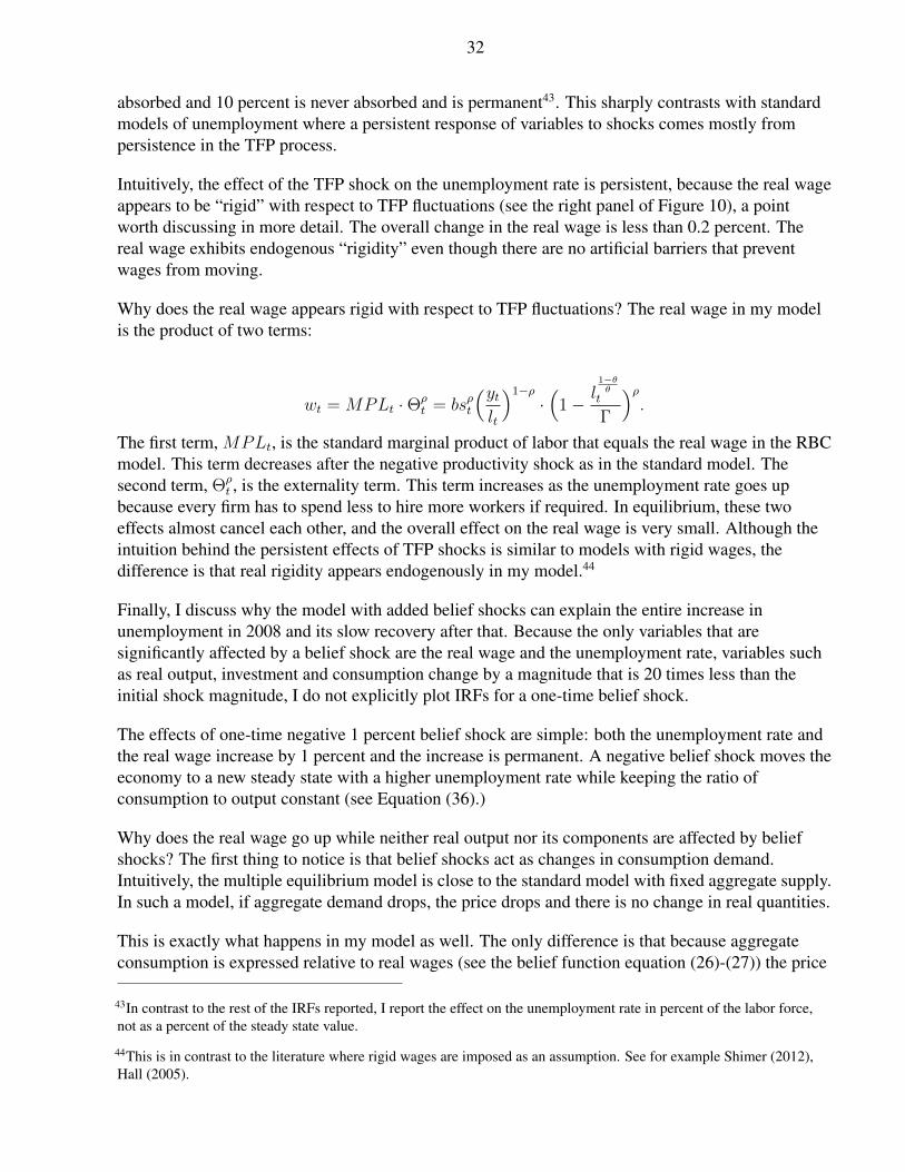
32

absorbed and 10 percent is never absorbed and is permanent43. This sharply contrasts with standardmodels of unemployment where a persistent response of variables to shocks comes mostly frompersistence in the TFP process.

Intuitively, the effect of the TFP shock on the unemployment rate is persistent, because the real wageappears to be “rigid” with respect to TFP fluctuations (see the right panel of Figure 10), a pointworth discussing in more detail. The overall change in the real wage is less than 0.2 percent. Thereal wage exhibits endogenous “rigidity” even though there are no artificial barriers that preventwages from moving.

Why does the real wage appears rigid with respect to TFP fluctuations? The real wage in my modelis the product of two terms:

wt = MPLt ·Θρt = bsρt

(ytlt

)1−ρ·(

1− l1−θθ

t

Γ

)ρ.

The first term, MPLt, is the standard marginal product of labor that equals the real wage in the RBCmodel. This term decreases after the negative productivity shock as in the standard model. Thesecond term, Θρ

t , is the externality term. This term increases as the unemployment rate goes upbecause every firm has to spend less to hire more workers if required. In equilibrium, these twoeffects almost cancel each other, and the overall effect on the real wage is very small. Although theintuition behind the persistent effects of TFP shocks is similar to models with rigid wages, thedifference is that real rigidity appears endogenously in my model.44

Finally, I discuss why the model with added belief shocks can explain the entire increase inunemployment in 2008 and its slow recovery after that. Because the only variables that aresignificantly affected by a belief shock are the real wage and the unemployment rate, variables suchas real output, investment and consumption change by a magnitude that is 20 times less than theinitial shock magnitude, I do not explicitly plot IRFs for a one-time belief shock.

The effects of one-time negative 1 percent belief shock are simple: both the unemployment rate andthe real wage increase by 1 percent and the increase is permanent. A negative belief shock moves theeconomy to a new steady state with a higher unemployment rate while keeping the ratio ofconsumption to output constant (see Equation (36).)

Why does the real wage go up while neither real output nor its components are affected by beliefshocks? The first thing to notice is that belief shocks act as changes in consumption demand.Intuitively, the multiple equilibrium model is close to the standard model with fixed aggregate supply.In such a model, if aggregate demand drops, the price drops and there is no change in real quantities.

This is exactly what happens in my model as well. The only difference is that because aggregateconsumption is expressed relative to real wages (see the belief function equation (26)-(27)) the price

43In contrast to the rest of the IRFs reported, I report the effect on the unemployment rate in percent of the labor force,not as a percent of the steady state value.

44This is in contrast to the literature where rigid wages are imposed as an assumption. See for example Shimer (2012),Hall (2005).

33

corresponds to the inverse of the real wage. Therefore, a price drop implies an increase in the realwage.

In my model the unemployment rate exhibits hysteresis. These dynamics explain the phenomenonthat has been dubbed “jobless recoveries” – a high persistent unemployment rate and real growth atthe same time. To see this, consider a negative belief shock. In response to a shock of this kind,unemployment will rise proportionally and stay high for a potentially infinite period of time. At thesame time there will be no decrease in real output, consumption, or investment. If a positiveproductivity shock follows such a belief shock, the economy will converge back to a new steady statewith the new higher unemployment rate.

In my model a negative belief shock causes an increase in real wages. This is what we observe in thedata. Between 2006 and 2011, real hourly earnings increased by around 3 percent while hoursworked and the employment rate dropped significantly (see Kocherlakota (2012)).

VI. CONCLUSION

In this paper I constructed and estimated a general equilibrium rational expectations model thatdisplays hysteresis in unemployment as in Blanchard and Summers (1987). My model can explainboth “jobless” or post-1990 recoveries as well as postwar U.S recoveries prior to 1990.

My model has the potential to explain the prolonged increase in the unemployment rate that weobserved in the U.S. after the Great Recession as a socially inefficient equilibrium outcome.Additionally, the model can reproduce stylistic business cycle dynamics in output, consumption,investment and real wages over the entire postwar period. In particular, in contrast to nearly all laborsearch models, in my model real wages are slightly countercyclical as in the data.

My model advances on two other branches of the literature. First, it expands second generationendogenous business cycle models to include the behavior of investment, consumption and realwages together with output and unemployment.45 Second, it provides deeper micro-foundations forwhy real wages are rigid with respect to a TFP shock. In contrast to the existing rigid wagesliterature (see Hall (2005), Shimer (2005)), I obtain this property of the real wage without directlyimposing an assumption of nominal or real rigidity.

My model is driven by two shocks: a TFP shock that explains fluctuations at business cyclefrequencies and a belief shock that explains permanent shifts in the unemployment rate. Productivityshocks have similar transitory effects as in a standard model. But they also have long-lasting effectson the unemployment rate, produced by an endogenous propagation mechanism. Together, demandand supply shocks generate jobless recoveries, and a high persistent unemployment rate can coexistwith positive real growth.

The model does not contradict the view that productivity shocks are a major source of economicfluctuations as in Nelson and Plosser (1982) and Long and Plosser (1983). Rather the model enrichesthis view by combining it with the idea that the unemployment rate displays the property ofhysteresis.

45See Farmer (2012a) for a recent review of endogeneous business cycle literature

34

I find that neither demand nor supply shocks alone can explain the observed dynamics ofemployment and GDP in the postwar data. With no demand disturbances one is likely to comeacross an “unemployment volatility puzzle” because the unemployment rate is a lot more volatilethan the data generated by the model. With no TFP shocks the model cannot explain the observedvolatility of investment.

What is a belief shock? Farmer (2012b) argues that the stock market crash of 2008 was similar innature to what Keynes (1936) referred to as “animal spirits”. Stock market wealth and housingwealth both fell sharply in 2008. This drop in wealth, caused by self-fulfilling shock to beliefs aboutpermanent income, can partially explain the Great Recession.

35

REFERENCES

Adjemian, Stephane, Houtan Bastani, Michel Juillard, Ferhat Mihoubi, George Perendia, MarcoRatto, and Sebastien Villemot, 2011, “Dynare: Reference Manual, Version 4,” Dynare WorkingPapers, CEPREMAP, Vol. 1.

An, Sungbae, and Frank Schorfheide, 2007, “Bayesian analysis of DSGE models,” EconometricReviews, Vol. 6, pp. 113-172.

Ball, Laurence, 2009, “Hysteresis in Unemployment: Old and New Evidence,” NBER WorkingPapers 14818.

Benhabib, Jess, and Roger E. A. Farmer, 1994, “Indeterminacy and Increasing Returns,” Journal ofEconomic Theory, Vol. 63, pp. 19-46.

Berger, David, 2013, “Countercyclical Restructuring and Jobless Recoveries,” Northwestern mimeo.

Blanchard, Olivier, and Jordi Gali, 2008, “Labor Markets and Monetary Policy: A New-KeynesianModel with Unemployement,” MIT Department of Economics Working Paper, Vol. No. 06-22.

Blanchard, Olivier J., and Danny Quah, 1989, “The Dynamic Effects of Aggegrate Demand andSupply Disturbances,” The American Economic Review, Vol. 79, pp. 655–673.

, and Lawrence H. Summers, “Hysterisis and the European Unemployment Problem,” 1986,in “NBER Macroeconomics Annual,” Vol. 1 (National Bureau of Economic Research),pp. 15–90.

, and , 1987, “Hysterisis in Unemployment,” European Economic Review, Vol. 31, pp.288-295.

Blundell, Richard, and Thomas H. MaCurdy, 1999, “Labor Supply: A Review of AlternativeApproaches,” Handbook of Labor Economics, Vol. 3, pp. 1559-1695.

Chari, V. V., Patrick Kehoe, and Ellen McGrattan, 2007, “Business Cycle Accounting,”Econometrica, Vol. 75, No. 3, pp. 781-836.

Evans, George W., and Gary Ramey, 2006, “Adaptive Expectations, Underparameterization and theLucas Critique,” Journal of Monetary Economics, Vol. 53, pp. 249-264.

, and Seppo Honkapohja, 1993, “Adaptive forecasts, hysteresis and endogenous fluctuations,”Federal Reserve Bank of San Francisco Economic Review, Vol. 1, pp. 3-13.

, and , 2000, “Expectations and the Stability Problem for Optimal Monetary Policies.”University of Oregon, mimeo.

Farmer, Roger, Carine Nourry, and Alain Venditti, 2013, “The Inefficient Markets Hypothesis: WhyFinancial Markets Do Not Work Well in the Real World,” NBER Working paper 18647.

Farmer, Roger E. A., 2002, “Why Does the Data Reject the Lucas Critique?,” Annales d’Economie etde Statistiques, No. 67-68, pp. 111-129.

, 2006, “Old Keynesian Economics,” UCLA mimeo.

36

, 2010, Expectations, Employment and Prices (Oxford University Press).

, 2011, “Animal Spirits, Rational Bubbles and Unemployment in an Old-Keynesian Model,”NBER WP 17137.

, 2011, “Confidence, Crashes and Animal Spirits,” Economic Journal.

Farmer, Roger E A, 2012, “The Evolution of Endogenous Business Cycles,” CEPR Discussion Paper9080.

, 2012, “The stock market crash of 2008 caused the Great Recession: Theory and evidence,”Journal of Economic Dynamics & Control, Vol. 36, pp. 693-707.

, and Dmitry Plotnikov, 2012, “Fiscal policy in the model with hysteresis,” UCLA mimeo.

Farmer, Roger E. A., and Jang Ting Guo, 1994, “Real Business Cycles and the Animal SpiritsHypothesis,” Journal of Economic Theory, Vol. 63, pp. 42-73.

Fernandez-Villaverde, Jesus, and Juan Rubio-Ramirez, 2005, “Comparing Dynamic EquilibriumModels to Data: A Bayesian Approach,” Journal of Econometrics, Vol. 123, pp. 891–910.

, and , 2005, “Estimating Dynamic Equilibrium Economies: Linear VersusNon-Linear Likelihood,” Journal of Applied Econometrics, Vol. 20, pp. 891-910.

Friedman, Milton, 1957, A Theory of the Consumption Function (Princeton University Press).

Galı, Jordi, Frank Smets, and Rafael Wouters, 2012, “Slow Recoveries: A Structural Interpretation,”Journal of Money, Credit and Banking, Vol. 44 (2), pp. 9-30.

Hall, Robert E., 2005, “Employment Fluctuations with Equilibrium Wage Stickiness,” AmericanEconomic Review, Vol. 95, No. 1 (March), pp. 50-65.

Hall, Robert E, 2011, “The Long Slump,” American Economic Review, Vol. 101(2), pp. 431-69.

Hansen, Gary D., 1985, “Indivisible Labor and the Business Cycle,” Journal of MonetaryEconomics, Vol. 16, pp. 309-327.

Jaimovich, Nir, and Henry Siu, 2013, “The Trend is the Cycle: Job Polarization and JoblessRecoveries,” Duke mimeo.

Jong, Piet De, 1991, “The Diffuse Kalman Filter,” The Annals of Statistics, Vol. Volume 2, No 2, pp.1073-1083.

Justiniano, Alejandro, Giorgio E. Primiceri, and Andrea Tambalotti, 2010, “Investment Shocks andBusiness Cycles,” Journal of Monetary Economics, Vol. 57, pp. 132-145.

Keynes, John Maynard, 1936, The General Theory of Employment, Interest and Money (MacMillanand Co.).

Klump, Rainer, Peter McAdam, and Alpo Willman, 2007, “Factor Substitution andFactor-Augmenting Technical Progress in the United States: a Normalized Supply-Side SystemApproach,” The Review of Economics and Statistics, Vol. 89(1), pp. 183-192.

37

Kocherlakota, Narayana, 2012, “Incomplete Labor Markets,” Research Papers of MinneapolisFederal Reserve.

Koopman, Siem Jan, 1997, “Exact Initial Kalman Filtering and Smoothing for Nonstationary TimeSeries Models,” Journal of the American Statistical Association, Vol. 92, No. 440 (Dec., 1997),pp. 1630-1638.

, and James Durbin, 2000, “Fast Filtering And Smoothing For Multuvariate State SpaceModels,” Journal of Time Series Analysis, Vol. 21, No. 3, pp. 281-296.

Long, John B, and Charles I. Plosser, 1983, “Real Business Cycles,” Journal of Political Economy,Vol. 91, No. 1, pp. 39-69.

Ludvigson, Sidney C., and Martin Lettau, 2004, “Understanding Trend and Cycle in Asset Values:Reevaluating the Wealth Effect on Consumption,” American Economic Review, Vol. 94, No. 1,pp. 277-299.

Mortensen, Dale T., and Eva Nagypal, 2007, “More on Unemployment and Vacancy Fluctuations,”Review of Economic Dynamics, Vol. 10, pp. 327-347.

Muth, John F., 1961, “Rational Expectations and the Theory of Price Movements,” Econometrica,Vol. 29, pp. 315-335.

Nadiri, M. Ishaq, and Ingmar R. Prucha, 1997, “Estimation of the Depreciation Rate of Physical andR&D Capital in the U.S. Total Manufacturing Sector,” NBER Working Paper No. 4591.

Nelson, Charles R., and Charles Plosser, 1982, “Trends and random walks in macroeconomic timeseries: Some evidence and implications,” Journal of Monetary Economics, Vol. 10, pp.139-162.

Plotnikov, Dmitry, 2012, “Can an RBC model match medium-term business cycle fluctuations in theU.S. data?,” UCLA working paper.

Reinhart, Carmen, and Kenneth Rogoff, 2009, This Time is Different (Princeton University Press).

Rogerson, Richard, Robert Shimer, and Randall Wright, 2005, “Search-Theoretic Models of theLabor Market: A Survey,” Journal of Economic Literature, Vol. 43, pp. 959-988.

Shiller, Robert J., 2000, Irrational Exuberance (Princeton University Press).

Shimer, Rober, 2012, “Wage Rigidities and Jobless Recoveries,” Journal of Monetary Economics,Vol. 59(Supplement), pp. S65-S77.

Shimer, Robert, 2005, “The Cyclical Behavior of Equilibrium Unemployment and Vacancies,”American Economic Review, Vol. 95, No. 1, pp. 25-49.

Sims, Christopher A., 2001, “Solving Linear Rational Expectations Models,” Journal ofComputational Economics, Vol. 20, No. 1-2, pp. 1-20.

Wiczer, David, 2013, “Long-Term Unemployment: Attached and Mismatched?,” University ofMinnesota Working Paper.