HYPERSEEING - ISAMA Homepage · For inclusion in Hyperseeing, au-thors are invited to email...

HYPERSEEINGEditors. Ergun Akleman, Nat Friedman.

Associate Editors. Javier Barrallo, Anna Campbell Bliss, Benigna Chilla, Michael Field, Slavik Jablan, Steve Luecking, John Sullivan, Elizabeth Whiteley.

Page Layout. Ergun Akleman

FALL 2011 - WINTER 2012

Cover Image: Gabriele Meyer’s Crotchet Sculpture: Hyperbolic Disk

Article Submission

For inclusion in Hyperseeing, au-thors are invited to email articles for the preceding categories to:

hyperseeing at gmail.comnat.isama77 at gmail.comergun.akleman at gmail.com

Articles should be a maximum of eight pages.

Articles

Crocheting Hyperbolic Surfacesby Gabriele Meyer

Keizo Ushio: 2010 and 2011by Nat Friedman & Ergun Akleman

Statistical Geometry in One Dimensionby John Shier

Serial Polar Transforma-tions Of Simple Geometries IIby Leo S. Bleicher

Eva Hild: Large-scale Sculpturesby Nat Friedman

Recent 3D Printed Sculp-turesby Henry Segerman

Sculptural Forms of Wire Pass, Buckskin Gulch and Zebra Slotby Robert Fathauer

Cartoons

MADmatic by Ergun Akleman

Announcements

ISAMA 2012Chicago June 18-22

ISAMAwww.isama.org

The International Society of the Arts, Mathematics, and Architecture

BECOME A MEMBER

ISAMA Membership Registration

Membership in ISAMA is free. Membership implies you will receive all ISAMA email announcements concerning conferences and other news items of interest.

Name………………………………………………………………………………………………………………….

Address……………………………………………………………………………………………………………………………………………………………………………………………………………………………………………………………………………………………………………………………………………………………………………………………………………………………………………………………………………………………………………………………………………………………………………………………………………………………………………………………………………………………………………………………………………………………

Email address…………………………………………………………………………………………………………………………….

Interests…………………………………………………………………………………………………………………………………………………………………………………………………………………………………………………………………………………………………………………………………………………………………………………………………………………………………………………………………………………………………………………………………………………………………………………………………………………………………………………………………………………………………………………………………………………………………………………………………………………………………………………………………………………………………………………

Please email completed form to Nat Friedman at [email protected]

BECOME A MEMBER

ISAMA 2012 Announcement

Eleventh Interdisciplinary Conference of the International Society of the

Arts, Mathematics and Architecture

June 18-22, 2012

ISAMA 2012 will be held June 18-22, 2012 at DePaul University co-organized with Steve Luecking and the Illinois Institute of Technology (IIT), co-organized with Robert Krawczyk. ISAMA 2012 celebrates the 20th anniversary of the first Art and Mathematics Conference AM92, organized by Nat Friedman at the University at Albany, New York in June, 1992.

CrochetingÊ HyperbolicÊ Surfaces Gabriele Meyer

Department of Mathematics University of Wisconsin, Madison

Madison, WI 53706 Email: [email protected]

Website:Ê http://www.math.wisc.edu/~meyer/ A hyperbolic surface is characterized by the property, that locally, in the vicinity of each point, it looks like a saddle. So it is definitely not a flat surface. You will only get a very crude approximation, if you try to model it out of flat pieces of cardboard. This dilemma was already noticed centuries earlier, when the first map makers tried to faithfully depict the globe (mathematical sphere) on a flat sheet of paper. Trying to do that introduces distortions that will either make the landmasses near the north and south pole appear larger or the regions near the equator appear smaller than they are relative to land masses elsewhere. In essence we have discovered spherical, flat and hyperbolic geometry.

Figures 1-4. evolution of a hyperbolic disk

It is possible to create hyperbolic surfaces out of wood, metal, clay, glass and plastic, but all these methods have so far only created surfaces of limited extent, simply because the curvy nature makes many places on the surface hard to reach. So what is a relatively “natural” way of creating these surfaces? If you crochet a small flat disk by working in a spiral from the inside out, and then, rather than making the right number of stitches around the perimeter, you make a few more than you actually need, this will cause the surface to become wavy around the perimeter. Eventually the waves become significant and you have created a saddle. If you keep increasing the number of stitches, say for every 8th stitch you make an

additional stitch (into the same place where you made the eighth), then this will create a hyperbolic surface. If you make fewer than the necessary number of stitches, in other words you leave a gap, the surface will be spherical, if you make just the right number of stitches, then the surface will become flat.

This idea of creating hyperbolic surfaces was first put in practice by mathematicians/artists: Hinke M. Osinga & Bernd Krauskopf [1], Carlos Sequin [2], and Eva Hild [3] in the early 2000s. I learned it from Daina Taimina [4] at Cornell University through her husband David Henderson, who was my Ph.D. advisor.

Figure 5. A white hyperbolic disk Figure 6: This surface consists of five hyperbolic half planes attached to each other at the top and the bottom. Creating this one involved a lot of counting. This could be used as a lamp shade, because it has empty space in the center.

ISAMA Crocheting HyperbolicÊ SurfacesGabriele Meyer

Department of MathematicsUniversity of Wisconsin, Madison

Madison, WI 53706Email: [email protected]

Website:Ê http://www.math.wisc.edu/~meyer/

BECOME A MEMBER




June 18-22, 2012


Figure 7: Red flame is a red algae. Here I actually tried to crochet a wave pattern into the screw shape, It involves a lot of counting. Figure 8: Several hyperbolic surfaces: an asymmetric green algae, a hyperbolic disk, and a red hyperbolic half plane, with a small spherical shape and a small hyperbolic disk attached. Figure 9: Algaen tower is a large white hyperbolic disk, experiment with stitches of various lengths.

Figure 10. A white hyperbolic disk, that is used as a lamp shade (fire hazard, unless you use energy efficient, low watt bulbs). I experimented with triple stitches here. Figure 11: Three hyperbolic half planes attached at the top and the bottom, used as a lamp shade. Figure 12: Red hyperbolic disk is a tower of hyperbolic disks and a white algae.

Figure 13. Largest white. Figure 14. Red blossom: You start this one from the end of the stem and gradually increase the stitches until you get to the place where it flares. There you increase the stitches more rapidly. This idea was also taken up by Christine and Margaret Wertheim [5], from the Institute For Figuring, who saw a connection to sea creatures and in collaboration with many enthusiastic women crocheted coral reefs, which were widely exhibited in the US and overseas. Hyperbolic surfaces occur frequently in nature: in the shapes of corals, salad leaves, leaves in general, blossoms, jelly fish, etc. My aim was to make hyperbolic crochet surfaces that kept their shape and would not flop, as crochet objects usually do. After some attempts with willow branches (they broke) and clothes line (too thick, but generally the right idea), I crochet in weed whacker line, which works perfectly. The surface becomes firm, but not hard, won’t weigh much, doesn’t hurt when you bump into it and looks pretty! The technique makes this something new, in between crocheting and basket making. You are now ready to embark on your own discovery tour of the world of hyperbolic surfaces. Here are some, which I made over the course of the last five years. Sofar I have made three basic types of surfaces:

the hyperbolic disk, the blossom, which has a long stem, and the algae, which consists of two hyperbolic half planes attached to each other, a simplified version

of that is the screw.

Other, more random shapes are no doubt possible.

References: [1] Hinke M. Osinga & Bernd Krauskopf, Crocheting the Lorenz Manifold, The Mathematical Intelligencer 26(4) (2004) 25-37

[2] Sculpture Designs by Carlo H. Séquin, Scherk Collins Toroids, http://www.cs.berkeley.edu/~sequin/SCULPTS/SEQUIN/scherkcollins.html [3] Eva Hild: Topological Sculpture from Life Experience, http://math.albany.edu/math/pers/artmath/art/eh.html [4] Daina Taimina’s webpage: http://www.math.cornell.edu/~dtaimina/ [5] Webpage of the Institute For Figuring: http://www.theiff.org/

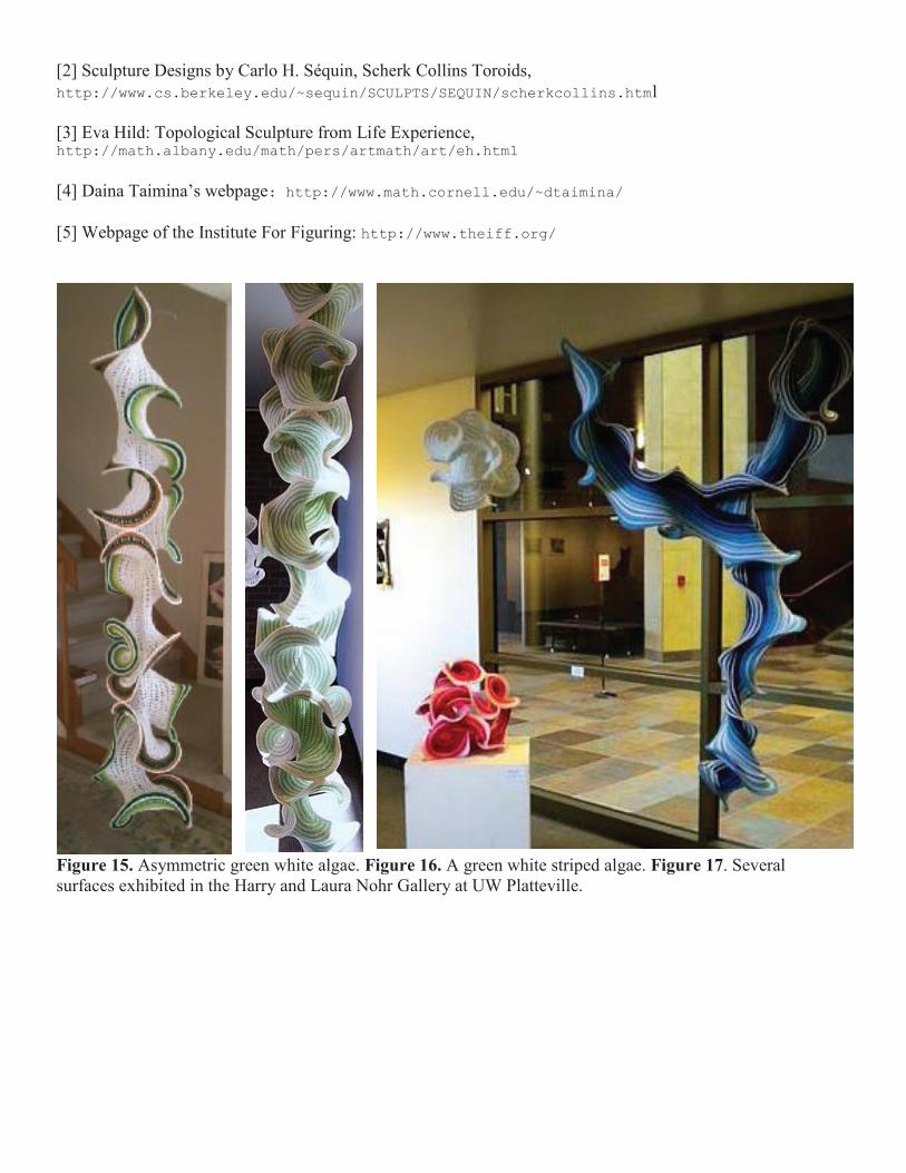
Figure 15. Asymmetric green white algae. Figure 16. A green white striped algae. Figure 17. Several surfaces exhibited in the Harry and Laura Nohr Gallery at UW Platteville.

[2] Sculpture Designs by Carlo H. Séquin, Scherk Collins Toroids, http://www.cs.berkeley.edu/~sequin/SCULPTS/SEQUIN/scherkcollins.html [3] Eva Hild: Topological Sculpture from Life Experience, http://math.albany.edu/math/pers/artmath/art/eh.htmlÊ

[4] Daina Taimina’s webpage:Ê http://www.math.cornell.edu/~dtaimina/ [5] Webpage of the Institute For Figuring: http://www.theiff.org/

Figure 15. Asymmetric green white algae. Figure 16. A green white striped algae. Figure 17. Several surfaces exhibited in the Harry and Laura Nohr Gallery at UW Platteville.

Keizo Ushio: 2010 and 2011

Nat Friedman & Ergun Akleman

Introduction This paper presents the works of Japanese sculptor Keizo Ushio in 2010 and 2011 including several installations of earlier sculptures. Keizo was quite active in these two years. In both years he participated in group sculpture exhibits at Bondi Beach and Cottesloe in Australia, as well as a group exhibit in 2011 in Aarhus, Denmark. He has a one-year outdoor solo show consisting of four sculptures in Stockholm, Sweden until April, 2012. Keizo installed four sculptures in Australia at Bondi Beach, Margaret River, Perth, and Newman. Keizo also installed three sculptures in Japan at Diplomatic establishments of Hyogo in Kobe, Kita-Nagoya City, and Takumina Corporation, Asago City. Hopefully the four sculptures exhibited in Stockholm will be moved to Chicago, USA, to be exhibited at the conference ISAMA 2012, June 18-22, 2012.Keizo will also be carving a sculpture in Chicago that he plans to complete during the conference. For more information about Keizo work you can refer the book [1], whichgives a complete discussion of his works up to 2008. His works are also discussed in [2-4]. Here the works of 2010 and 2011 are discussed

2010 Exhibits and Installations Bondi Beach Exhibit 2010

Figure 1. Oushi Zokei 2010 Circle, Japanese black granite, 2010, 192 x 188 x 150 cm. Figure 2. Linking up in Oushi Zokei Circle 2010. Figure 3. Oushi Zokei Circle 2010, detail.

Keizo had a sculpture in Bondi Beach, Sydney, Australia, called Sculpture by the Sea 2010 (see Figure 1). This sculpture became a center of attention for children who enjoyed the sculpture as seen in Figure 2. A detail shot is shown in Figure 3. Keizo also had four sculptures in the indoor exhibit at Bondi Beach, as shown below. In Figure 4 is a divided Mobius in beautiful polished Norwegian granite. In the same granite, in Figure 5 is a smaller version of the sculpture in Figure 1. For a change, Keizo carved two scuptures in white marble shown in Figure 6. These are variations on the divided Mobius.

Figure 4. Oushi Zokei E-1, Norwegian emerald pearl granite, 2010, 42 x 43 x 13 cm. Figure 5. Oushi Zokei E-3, Norwegian emerald pearl granite, 2010, 47x 48x 18cm, Sydney AU, private collection. Figure 6. (lower left) Oushi Zokei 2009 – stretch up, white marble, 2009, 42x 35x 16 cm, private collection. (upper right) Oushi Zokei 2009 – Laurel, white marble, 2009, 35x 35 x 16 cm, artist’s collection. Kita Nagoya City Sculpture Competition Keizo’s entry in the 2010 Kita Nagoya City Sculpture Competition is the sculpture in African black granite shown in Figure 7. This is a torus with a triple twist Mobius space resulting in a trefoil knotted form. The surface is finished roughly and the drill marks have been refined as seen in the detail shot in Figure 8. The sculpture was purchased by the city and its setting is Kita Nagoya City, Japan. Sculpure by the Sea Cottesloe 2010 Keizo’s sculpture in the 2010 group exhibit at Cottesloe is shown in Figure 9. This was a new form for Keizo. It is a vertical form with mirror symmetry about the center line. It is representative of a Japanese traditional dish. It is now in a private collection in Perth. Another view is shown in Figure 10 with Keizo at the front left with several other Japanese sculptors.

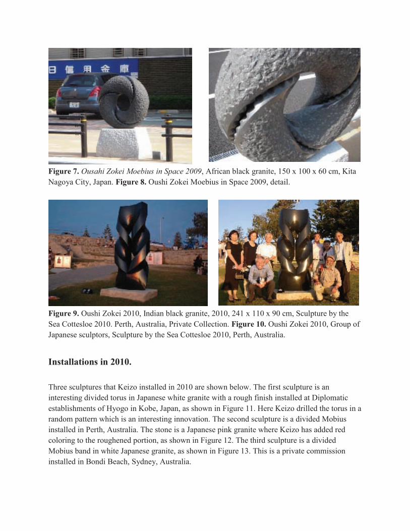
Figure 7. Ousahi Zokei Moebius in Space 2009, African black granite, 150 x 100 x 60 cm, Kita Nagoya City, Japan. Figure 8. Oushi Zokei Moebius in Space 2009, detail.

Figure 9. Oushi Zokei 2010, Indian black granite, 2010, 241 x 110 x 90 cm, Sculpture by the Sea Cottesloe 2010. Perth, Australia, Private Collection. Figure 10. Oushi Zokei 2010, Group of Japanese sculptors, Sculpture by the Sea Cottesloe 2010, Perth, Australia.

Installations in 2010. Three sculptures that Keizo installed in 2010 are shown below. The first sculpture is an interesting divided torus in Japanese white granite with a rough finish installed at Diplomatic establishments of Hyogo in Kobe, Japan, as shown in Figure 11. Here Keizo drilled the torus in a random pattern which is an interesting innovation. The second sculpture is a divided Mobius installed in Perth, Australia. The stone is a Japanese pink granite where Keizo has added red coloring to the roughened portion, as shown in Figure 12. The third sculpture is a divided Mobius band in white Japanese granite, as shown in Figure 13. This is a private commission installed in Bondi Beach, Sydney, Australia.

Figure 11. Oushi Zokei Random, Japanese white granite, 2008, 120x 180x 50 cm, Asago art festival 2008 , Hyogo,Japan, Installed 2010 at Diplomatic establishments of Hyogo in Kobe, Japan. Figure 12. Oushi Zokei 2009 Moebius in space, Japanese pink granite, 183 x 183 x 60 cm (without base) Sculpture by the Sea Cottesloe 2009, Perth, AU, Installed 2010 at the Esplanade station Perth AU. Figure 13. Oushi Zokei 2010 Moebius in space, Japanese white granite, 2010 70 x 70 x 30 cm, Commission for private collection in Bondi Beach, Sydney AU.

Arts Cape Biennial 2010 Keizo is shown in Figure 14 with his sculpture exhibited in the Arts Cape Biennial 2010 Byron Bay NSW, Australia. This is a new version of a divided Mobius embedded in the stone and in a slanted position. A second view is shown with a new friend in Figure 15.

Figure 14. Keizo with Oushi Zokei Mobius In Space Rising, 2009, 115 x 105 x 50 cm. Japanese Black Granite. Figure 15. Oushi Zokei Mobius In Space Rising with new friend.

Figure 11. Oushi Zokei Random, Japanese white granite, 2008, 120x 180x 50 cm, Asago art festival 2008 , Hyogo,Japan, Installed 2010 at Diplomatic establishments of Hyogo in Kobe, Japan. Figure 12. Oushi Zokei 2009 Moebius in space, Japanese pink granite, 183 x 183 x 60 cm (without base) Sculpture by the Sea Cottesloe 2009, Perth, AU, Installed 2010 at the Esplanade station Perth AU. Figure 13. Oushi Zokei 2010 Moebius in space, Japanese white granite, 2010 70 x 70 x 30 cm, Commission for private collection in Bondi Beach, Sydney AU.

Arts Cape Biennial 2010 Keizo is shown in Figure 14 with his sculpture exhibited in the Arts Cape Biennial 2010 Byron Bay NSW, Australia. This is a new version of a divided Mobius embedded in the stone and in a slanted position. A second view is shown with a new friend in Figure 15.

Figure 14. Keizo with Oushi Zokei Mobius In Space Rising, 2009, 115 x 105 x 50 cm. Japanese Black Granite. Figure 15. Oushi Zokei Mobius In Space Rising with new friend.

Sculptures and Installations 2011 Solo Exhibit in Stockholm Keizo had an outdoor solo exhibit in Stockholm, Sweden consisting of four large sculptures shown below. The first is shown in Figure 16.It is a vertical divided double twist band that separates into two intertwined forms.

Figure 16. Oushi Zokei 2006, Blue granite, 150 x 350 x 90 cm (without base). Figure 17. Oushi Zokei 2004, Blue granite, 450 x 165 x 90 cm. Figure 18. Alternate view of Oushi Zokei 2004.

The second sculpture is a horizontal divided double twist band shown in Figure 17. This sculpture also separates into two intertwined forms. An alternate view is shown in Figure 18. Note that the two bands in Figures 16 and 17 both separate into two intertwined forms but they are quite different shapes. In both cases the space is a double twisted space. The third sculpture is a divided

Mobius shown in Figure 19. This is a divided single twist Mobius. The surface treatment has a polished part on top and contrasting rough sections below. It is a colorful granite with red and

Figure 19. Mobius in Space 2005, colored granite, 200 x 220 x 120 cm. Figure 20. Seven cubes, blue granite, 130 x 420 x 90 cm (without base).

white stripes. The fourth sculpture is a cubic construction shown on the left in Figure 20. This sculpture was carved from one piece of stone.

Sculpture by the Sea, Bondi Beach 2011. Keizo’s sculpture in the 2011 Bondi Beach outdoor exhibit is shown in Figure 21. It is a smooth divided single twist Mobius. The new innovation is the set of small stones inserted in the Mobious space. An alternate view is shown in Figure 22.

INNOVATION Keizo placed a commissioned work INNOVATION at the Takumina Corporation in the city of Asago, Japan. The following sequence of images show the development of the sculpture from measuring the block to the unveiling and final placement.

Figure 23. Keizo measuring the block. Figure 24. Beginning stage of carving. Figure 25. Advanced stage of carving. Figure 26. Drilling holes to form dividing space. Figure 27. Placing completed sculpture on its base. Figure 28. Unveiling ceremony of Innovation, Keizo is second from left, November 9, 2011.

Figure 21. Mobius in Space 2011, Blue granite, 183 x 183 x 80 cm. Figure 22. Alternate view of Mobius in Space 2011 with a new friend.

Figure 29. Innovation, Pink granite, 240 x 200 x 120 cm, Takumina Corporation, Asago City, Japan. Innovation is a divided single twist Mobius. The shape is similar to a granite Mobius by Max Bill.In addition to dividing the Mobius, Keizo’s innovation is to emphasize the opposite curvatures of the two lower end parts so that the sculpture is quite three-dimensional.

Figure 30. Oushi Zokei 2009, Blue granite, 186 x 186 x 80 cm. Figure 31. Oushi Zokei 2009 with new friends. Figure 31a. Keizo’s drawing of sculture.

white stripes. The fourth sculpture is a cubic construction shown on the left in Figure 20. This sculpture was carved from one piece of stone.

Sculpture by the Sea, Bondi Beach 2011. Keizo’s sculpture in the 2011 Bondi Beach outdoor exhibit is shown in Figure 21. It is a smooth divided single twist Mobius. The new innovation is the set of small stones inserted in the Mobious space. An alternate view is shown in Figure 22.

INNOVATION Keizo placed a commissioned work INNOVATION at the Takumina Corporation in the city of Asago, Japan. The following sequence of images show the development of the sculpture from measuring the block to the unveiling and final placement.

Figure 23. Keizo measuring the block. Figure 24. Beginning stage of carving. Figure 25. Advanced stage of carving. Figure 26. Drilling holes to form dividing space. Figure 27. Placing completed sculpture on its base. Figure 28. Unveiling ceremony of Innovation, Keizo is second from left, November 9, 2011.

Figure 21. Mobius in Space 2011, Blue granite, 183 x 183 x 80 cm. Figure 22. Alternate view of Mobius in Space 2011 with a new friend.

Sculpture by the Sea, Aarhus 2011 Keizo participated in a group exhibit Sculpture by the Sea, Aarhus 2011 in Denmark. His sculpture is shown in Figure 30. A second image is shown in Figure 31 with new friends. The third image shows Kaizo’s drawing of sculpture. Arhus 2011 Indoor Exhibit

Keizo exhibited three smaller sculptures in the Arhus 2011 indoor exhibit. These are shown in below. An elegant vertical polished divided single twist Mobius is shown in Figure 32. A triple twist divided Mobius is shown in Figure 33. This form is a trefoil knot. The contrasting surface treatment is polished above and roughed out below. Here the sculpture and base are of one piece so it appears that the sculpture is rising out of the base. The sculpture in Figure 34 is a smaller version of the form in Figure 31 and is now in the private collection of the Danish Royal Family.

Figure 32. Oushi Zokei 2011 G-1 Gray granite, 28 x 60 x 16 cm. Figure 33. Oushi Zokei 2011 B-3 Black granite, 75 x 91 x 28 cm. Figure 34. Oushi Zokei 2011 R-3 Red granite, 48 x 47 x 17 cm. Vasse Felix Installation Vasse Felix is a winery in Margaret River, Western Australia that has a sculpture walk in a beautiful natural setting, as shown in Figure 35.

Keizo is shown in Figure 36 with the sculpture he installed at Vasse Felix in 2011. This is a painted divided torus that he carved in 2004. An alternate view is shown in Figure 37.

Figure 35. Vasse Felix Winery, Margaret River, Western Austalia. Figure 36. Oushi Zokei 2004, Acrylic paint on granite, 210 x 250 x 120 cm, The Holmes a’ Court Collection, Vasse Felix Winery, Margaret River, Western Australia. Figure 37. Oushi Zokei 2004, alternate view.

Sculpture by the Sea, Cottesloe 2011. Keizo also participated in the 2011 group exhibit on the beach at Cottesloe, Australia. His sculpture is shown in Figure 38. It is the vertical configuration of the divided torus.

Figure 38. Oushi Zokei 2008, Blue and brown granite, 200 x 280 x 200 cm, Private collection in Mosman Park WA, Australia. Figure 39. Oushi Zokei 2008, White granite, 380 x 280 x 260 cm. Figure 40. Alternate view of Oushi Zokei 2008. Installation in Newman, Australia.

Keizo is shown installing a divided torus sculpture in Figure 39 in Newman, Australia. A view of the installed sculpture is shown in Figure 40. Note the refined drill marks resulting from the splitting process, which are an impressive feature in bright sunlight. Thus the process results in strong visual effects.

References

[1] Oushi Zokei, Keizo Ushio, Text: Masakazu Horiuchi, David Handley, Nathaniel Friedman, Keizo Ushio, Dialogue: Tadayasu Sakai, Translation: Christopher Stephens, Nomart Editions, Osaka, Japan, 2008. [2] Nat Friedman, Keizo Ushio 2006, Part One, Hyperseeing, May, 2007. [3] Nat Friedman, Keizo Ushio 2006, Part Two, Hyperseeing, June, 2007. [4] Nat Friedman, Keizo Ushio: Recent Sculptures, Hyperseeing, Fall 2009. Issues of Hyperseeing can be seen at www.isama.org/hyperseeing/

Statistical Geometry in One Dimension

John Shier 6935 133rd Court

Apple Valley, MN, 55124, USA E-mail: [email protected]

Abstract

An algorithm which produces a family of Cantor-like one-dimensional random fractal-like structures on a line segment is described. Random numbers are a key feature.

1. Introduction; The Algorithm Stated

Fractals have come to be accepted in mathematics, physics, and several fields of practical application since the ground-breaking book by Mandelbrot [1]. A new random fractal-like1 structure in one dimension is described here. The name "statistical geometry" [3] was first used for the algorithm in two dimensions.

Figure 1: An example of the structure with c = 1.6. Several scales of detail are shown so that the reader can better grasp its form. The segments are the black regions, while the gasket is white. It can be seen in the top row that

many gasket gaps are wide enough for future segment placements. An understanding of the material presented requires a grasp of the rules for constructing these objects: 1 It has not yet been established whether this structure satisfies all the requirements of a fractal.

Statistical Geometry in One Dimension

John Shier 6935 133rd Court

Apple Valley, MN, 55124, USA E-mail: johnart@frart@frart@f ontiernontiernontier et.net

1. Create a sequence of line segment lengths λi following a power law, equal to

...,)3(

1,)2(

1,)1(

1,1cccc NNNN +++

where c and N are constant parameters. A line of

length L is to be filled with such segments.

2. Sum the lengths λi to infinity, using the Hurwitz zeta2 function

∑∞

= +=

0 )(1),(

iciN

Ncζ (1)

3. Define new lengths Li by

ci iNNcLL

))(,( +=ζ

(2)

It will be seen that the sum of these redefined lengths is L. 4. Let i = 0. Place a segment having length L0 in the length L at a random position x such that it falls entirely within length L. This is the "initial placement". Increment i. 5. Place a segment having length Li entirely within L at a random position x where it falls entirely within L. If this segment overlaps with any previously-placed segment repeat step 5. This is a "trial". 6. If this segment does not overlap with any previously-placed segment, store x and the segment length in the "placed segments" data base, increment i, and go to step 5. This is a "placement". 7. Stop when i reaches a fixed number, percentage filled reaches a fixed value, or other.

This is a very simple algorithm, easily stated in a few lines of text. Some might think it should be stated in terms of sets, but since what is actually reported are the results of computational experiments the results are described in those terms. All of the computations have been done with double-precision arithmetic. The parameters c and N can have a variety of values. In practice the parameter c is usually in the range 1.2-2.0. N can be 1 or larger, and need not be an integer. By construction the result appears to be a space-filling random fractal -- if the process never halts3. Available evidence (see below) says that it does not halt, at least for c values which are not close to the upper limit of usable c values.

2 The definitions of the Riemann and Hurwitz zeta functions can be found in Wikipedia. The Riemann zeta function is historically older than the Hurwitz function, and is the special case where N = 1. In my studies N is usually taken to be an integer, but according to the definition of ζ(c,N) it can be any real number ≥ 1. The Riemann zeta function has been much studied in connection with number theory, but it is not evident that such studies have any relevance here. 3 There are two ways to consider the halting question. One can ask whether the computational algorithm using floating-point numbers stops. Here the answer is probably yes, since there is a smallest feature size of 1 least-significant bit. Or one can ask whether the algorithm stops for ideal mathematical numbers, which have infinite

1. Create a sequence of line segment lengths λi following a power law, equal to

...,)3(

1,)2(

1,)1(

1,1cccc NNNN +++

where c and N are constant parameters. A line of

length L is to be filled with such segments.

2. Sum the lengths λi to infinity, using the Hurwitz zeta2 function

∑∞

= +=

0 )(1),(

iciN

Ncζ (1)

3. Define new lengths Li by

ci iNNcLL

))(,( +=ζ

(2)

It will be seen that the sum of these redefined lengths is L. 4. Let i = 0. Place a segment having length L0 in the length L at a random position x such that it falls entirely within length L. This is the "initial placement". Increment i. 5. Place a segment having length Li entirely within L at a random position x where it falls entirely within L. If this segment overlaps with any previously-placed segment repeat step 5. This is a "trial". 6. If this segment does not overlap with any previously-placed segment, store x and the segment length in the "placed segments" data base, increment i, and go to step 5. This is a "placement". 7. Stop when i reaches a fixed number, percentage filled reaches a fixed value, or other.

This is a very simple algorithm, easily stated in a few lines of text. Some might think it should be stated in terms of sets, but since what is actually reported are the results of computational experiments the results are described in those terms. All of the computations have been done with double-precision arithmetic. The parameters c and N can have a variety of values. In practice the parameter c is usually in the range 1.2-2.0. N can be 1 or larger, and need not be an integer. By construction the result appears to be a space-filling random fractal -- if the process never halts3. Available evidence (see below) says that it does not halt, at least for c values which are not close to the upper limit of usable c values.

2 The definitions of the Riemann and Hurwitz zeta functions can be found in Wikipedia. The Riemann zeta function is historically older than the Hurwitz function, and is the special case where N = 1. In my studies N is usually taken to be an integer, but according to the definition of ζ(c,N) it can be any real number ≥ 1. The Riemann zeta function has been much studied in connection with number theory, but it is not evident that such studies have any relevance here. 3 There are two ways to consider the halting question. One can ask whether the computational algorithm using floating-point numbers stops. Here the answer is probably yes, since there is a smallest feature size of 1 least-significant bit. Or one can ask whether the algorithm stops for ideal mathematical numbers, which have infinite

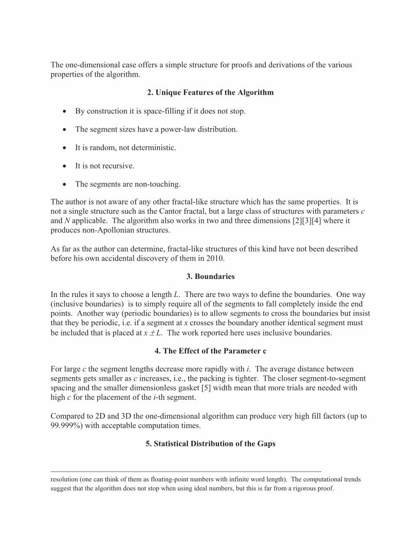
The one-dimensional case offers a simple structure for proofs and derivations of the various properties of the algorithm.

2. Unique Features of the Algorithm

• By construction it is space-filling if it does not stop.

• The segment sizes have a power-law distribution.

• It is random, not deterministic.

• It is not recursive.

• The segments are non-touching.

The author is not aware of any other fractal-like structure which has the same properties. It is not a single structure such as the Cantor fractal, but a large class of structures with parameters c and N applicable. The algorithm also works in two and three dimensions [2][3][4] where it produces non-Apollonian structures. As far as the author can determine, fractal-like structures of this kind have not been described before his own accidental discovery of them in 2010.

3. Boundaries In the rules it says to choose a length L. There are two ways to define the boundaries. One way (inclusive boundaries) is to simply require all of the segments to fall completely inside the end points. Another way (periodic boundaries) is to allow segments to cross the boundaries but insist that they be periodic, i.e. if a segment at x crosses the boundary another identical segment must be included that is placed at x ± L. The work reported here uses inclusive boundaries.

4. The Effect of the Parameter c For large c the segment lengths decrease more rapidly with i. The average distance between segments gets smaller as c increases, i.e., the packing is tighter. The closer segment-to-segment spacing and the smaller dimensionless gasket [5] width mean that more trials are needed with high c for the placement of the i-th segment. Compared to 2D and 3D the one-dimensional algorithm can produce very high fill factors (up to 99.999%) with acceptable computation times.

5. Statistical Distribution of the Gaps

resolution (one can think of them as floating-point numbers with infinite word length). The computational trends suggest that the algorithm does not stop when using ideal numbers, but this is far from a rigorous proof.

By gaps we mean the regions which make up the gasket (white regions in Fig. 1). With inclusive boundaries the parts of the gasket at the ends of L are also viewed as gaps. Before the initial placement there is just one gap of length L. The initial placement replaces this with two gaps. Each subsequent placement eliminates one gap and replaces it by two smaller ones. Thus after n placements the number of gaps will be n + 1.

Figure 2: A histogram of the gap widths. The vertical coordinate is the number of instances. The gray line

underneath shows the extent of the data. The largest gap lies in the farthest-right bin. The vertical gray line shows the width of the last-placed segment on the same x scale.

It can be seen that the data follows a decaying exponential trend. There are many gaps larger than the next-to-be-placed segment (vertical gray line), indicating that the algorithm will have no difficulty placing more segments. This is typical of the histograms for any c and any number of placed segments. There is a sparse population of quite large gaps, which are improbably numerous if this is truly an exponential p.d.f. There is a largest gap at any stage of the algorithm. The histogram of Fig. 2 is an estimate of a "master" probability distribution function p(c,n) of the gap widths, and indicates the form it takes. If one were to find a rigorous expression for p(c,n) as a function of c and n one could calculate most properties of the algorithm ab initio.

6. Run-Time Behavior What happens as the algorithm is executed? In particular, how many trials does it take to place some number of segments? How is this behavior affected by c? To this end one can plot log10(ncum) versus log10(n) where ncum(n) is the total number of trials needed to place n segments. Such a record will be different for each run.

• For large n, the data follows a straight line (see Fig. 3), showing that ncum(n) follows a power law in n, i.e.,

ncum(n) = Knf (3) The parameters K and f can be estimated from the data. They will have an uncertainty associated with the randomness of the process.

Figure 3: Run-time records. N = 1 in all cases. The vertical coordinate is log10(ncum) where ncum is the cumulative number of trials needed to place n segments. The horizontal coordinate is log10(n). From bottom to top, c = 1.2, 1.4, 1.6, 1.8, and 2.0. Three runs are plotted for each c value.

• For any number n of segments to be placed one can calculate an expected number m of

trials that will be needed. This is the basis for saying that the process does not halt. Although m may be huge, it is finite.

• For all of the c values on the graph, f ≅ c within statistical error.

• Lines fitted to the data appear to pass through the origin of (logarithmic) coordinates (0,0).

• The data becomes quite noisy for large c. It is thought that this noise sets the upper limit for usable c values.

7. Placement Probability

One can compute the placement probability for placement (n+1) by computing all of the gaps for n placements. One then determines which gaps are larger than the next-to-be-placed segment length. For these gaps, compute gap length minus next segment length and call it δx. Evidently the random x value must fall within a space of width δx for a placement to occur in this gap. The probability pplace that a placement occurs in any gap will be

L

xpplace

∑= δ (4)

Computations based on this are straightforward. Since this is a statistical estimate, the values found will have statistical scatter4. With c = 2.2 (N = 1) it was found that pplace ≅ .00028 for n = 323 placements, and that pplace ≅ .000080 for n = 922 placements. Taking the log slope between these two points one finds a value of 1.19. This probability is not the cumulative placement probability, which we have observed to have a log slope close to c (see above). The cumulative probability distribution for a given n will be the integral ∫dn of pplace(n), which would increase the log slope by 1, so that the log slope of ncum versus n would be 1.19 + 1 = 2.19. This is very close to the c value of 2.2 used in the algorithm. With these low placement probabilities, the distribution of the number of trials per placement should obey the Poisson distribution for rare events, which in this limit goes over to a decaying exponential function. This is in fact what is observed.

8. Fractal Dimension This section assumes that the structure will eventually be found to be fractal.

4 The statistical scatter in the probability thus computed is fairly small. Presumably is because the gaps are constrained by the overall requirement that they sum to the total gasket width, which is a non-random quantity.

• For any number n of segments to be placed one can calculate an expected number m of

trials that will be needed. This is the basis for saying that the process does not halt. Although m may be huge, it is finite.

• For all of the c values on the graph, f ≅ c within statistical error.

• Lines fitted to the data appear to pass through the origin of (logarithmic) coordinates (0,0).

• The data becomes quite noisy for large c. It is thought that this noise sets the upper limit for usable c values.

7. Placement Probability

One can compute the placement probability for placement (n+1) by computing all of the gaps for n placements. One then determines which gaps are larger than the next-to-be-placed segment length. For these gaps, compute gap length minus next segment length and call it δx. Evidently the random x value must fall within a space of width δx for a placement to occur in this gap. The probability pplace that a placement occurs in any gap will be

L

xpplace

∑= δ (4)

Computations based on this are straightforward. Since this is a statistical estimate, the values found will have statistical scatter4. With c = 2.2 (N = 1) it was found that pplace ≅ .00028 for n = 323 placements, and that pplace ≅ .000080 for n = 922 placements. Taking the log slope between these two points one finds a value of 1.19. This probability is not the cumulative placement probability, which we have observed to have a log slope close to c (see above). The cumulative probability distribution for a given n will be the integral ∫dn of pplace(n), which would increase the log slope by 1, so that the log slope of ncum versus n would be 1.19 + 1 = 2.19. This is very close to the c value of 2.2 used in the algorithm. With these low placement probabilities, the distribution of the number of trials per placement should obey the Poisson distribution for rare events, which in this limit goes over to a decaying exponential function. This is in fact what is observed.

8. Fractal Dimension This section assumes that the structure will eventually be found to be fractal.

4 The statistical scatter in the probability thus computed is fairly small. Presumably is because the gaps are constrained by the overall requirement that they sum to the total gasket width, which is a non-random quantity.

I have received box counting estimates of the fractal dimension D for the one-dimensional case from Paul Bourke [4]. This data fits reasonably well (within statistical uncertainty) to the formula5 D = 1/c (5) The largest usable c values appear to be around 2.7, which translates to a fractal D of .37.

9. The Dimensionless Gap Width Why does the algorithm work? One clue can be found from the dimensionless gap width. Suppose that L = 1 and assume N = 1. The total gasket width wg after n placements will

be ∑=

−=n

icg ic

nw1

1)(

11)(ζ

. The average gap width will be n

icnw

n

ic

gap

∑=

−= 1

1)(

11)( ζ . The

dimensionless one-dimensional gasket width6 b1(c,n) will be found by dividing this quantity by the length of segment n+1.

c

n

ic

ncnicncb

)1)((1

1)(

11),( 1

1 +

−=

∑=

ζζ (6)

When this is computed we find the following results for various n. c n=200 n=400 n=800 n=1600 n=3200 1.2 5.027500 5.013748 5.006873 5.003435 5.0017151.5 2.012503 2.006251 2.003126 2.001563 2.0007821.8 1.258759 1.254385 1.252203 1.251120 1.2505932.1 0.916166 0.912668 0.910967 0.910216 0.9100552.4 0.720289 0.717132 0.715302 0.713723 0.711181 The first noteworthy feature is the dependence on n. It is very weak. This indicates that the available space for placement of a new segment decreases at the nearly same rate as the segment size itself does. There is always room enough for another segment − at any n. The dependence on c is much stronger. As c increases the average gap width relative to the next-to-be-placed segment drops drastically. This helps to explain why the average number of trials per placement rises sharply with increasing c.

10. Summary

5 I suspect that this could be found in the literature if a sufficiently thorough search were made.

6 The two dimensional case is dealt with in an unpublished report [5]. By dimension we mean physical dimension. If meters are the length unit, b1(c,n) has units meters0.

The statistical geometry algorithm produces fractals in 1, 2, and 3 dimensions. The behavior of the algorithm is similar in all of these cases. Because of its simplicity the one-dimensional case has advantages for the development of detailed models and theories. A start has been made here in such a development. Statistical sampling has been used to show the general features of p(c,n) , ncum(c,n), and pplace(c,n). The author would like to thank Paul Bourke for many interesting discussions by electronic mail.

11. Conjectures and Problems Conjectures. Both of these are supported by computational experiments, but lack any proof. 1. The algorithm runs "to infinity" without stopping, with ideal mathematical numbers. 2. A power law is the sole, unique functional rule for segment length versus placed segment number if the result is to be space-filling. Problems. 1. Show that the mean or most probable value of f is c when N = 1.

12. References [1] Benoit Mandelbrot, Fractals: Form, Chance, and Dimension, W. H. Freeman & Co., 1977. [2] John Shier, Filling Space with Random Fractal Non-Overlapping Simple Shapes, Hyperseeing, Summer 2011 issue, pp. 131-140. [3] John Shier, Statistical Geometry, July 2011. A colorful self-published fractal art picture book available at lulu.com. [4] Paul Bourke's web site is paulbourke.net. The statistical geometry fractals are at paulbourke.net/texture_colour/randomtile/. Scroll to the bottom to see the 3D examples. [5] John Shier, The Dimensionless Gasket Width b(c,n) in Statistical Geometry (unpublished). Available at the author's web site john-art.com.

The statistical geometry algorithm produces fractals in 1, 2, and 3 dimensions. The behavior of the algorithm is similar in all of these cases. Because of its simplicity the one-dimensional case has advantages for the development of detailed models and theories. A start has been made here in such a development. Statistical sampling has been used to show the general features of p(c,n) , ncum(c,n), and pplace(c,n). The author would like to thank Paul Bourke for many interesting discussions by electronic mail.

11. Conjectures and Problems

Conjectures. Both of these are supported by computational experiments, but lack any proof.

1. The algorithm runs "to infinity" without stopping, with ideal mathematical numbers.

2. A power law is the sole, unique functional rule for segment length versus placed segment number if the result is to be space-filling.

Problems.

1. Show that the mean or most probable value of f is c when N = 1.

12. References

[1] Benoit Mandelbrot, Fractals: Form, Chance, and Dimension, W. H. Freeman & Co., 1977. [2] John Shier, Filling Space with Random Fractal Non-Overlapping Simple Shapes, Hyperseeing, Summer 2011 issue, pp. 131-140. [3] John Shier, Statistical Geometry, July 2011. A colorful self-published fractal art picture book available at lulu.com. [4] Paul Bourke's web site is paulbourke.net. The statistical geometry fractals are at paulbourke.net/texture_colour/randomtile/. Scroll to the bottom to see the 3D examples. [5] John Shier, The Dimensionless Gasket Width b(c,n) in Statistical Geometry (unpublished). Available at the author's web site john-art.com.

Serial Polar Transformations Of Simple Geometries II

Leo S. Bleicher

San Diego, CA 92037 [email protected]

Abstract

Complex shapes can be generated by repeated application of symmetry breaking geometric transformations to elementary shapes. Previous work has demonstrated the ability of the polar coordinate transformation used in conjunction with standard symmetry operations to create unusual and interesting forms. The appearance of these forms is dependent on the operations performed and the order of those operations; a wide variety of images may be generated from a single starting point. In this paper, additional transformation operations, longer sequences of transformations, various options for visualization, and a genetic algorithm for exploring these possibilities are described.

Introduction A previous communication1 outlined some of the elementary forms attainable by geometric transformation of simple shapes. Use of the standard symmetry operations of rotation, translation, scaling and reflection in the creation of patterns and tilings is one of the most ancient decorative methods. While repeated application of symmetry operations leave a shape unchanged from an aesthetic standpoint, interleaving these operations with symmetry-breaking transformations can rapidly lead to visually complex forms.2 In the previous study the polar coordinate transform was used exclusively as the symmetry breaking operation. In this paper access to additional classes of visual forms and patterns will be demonstrated through the inclusion of scaling operations, the inverse polar coordinate transform and circle inversion in the collection of operations, and through the use of longer transformation sequences. As transformation sequences become longer and more complex two artistic considerations need to be handled: sequence selection and visualization. Due to the combinatorial explosion of possible sequences exhaustive exploration quickly becomes impossible. While random generation of transformation sequences may generate interesting results, a better method is to use a directed search of the sequence space based on the aesthetic or novelty value of related sequences. One of the best methods for directing this type of search is a genetic recombination algorithm.3 Additionally, as sequences become longer, and the results more complex, the possible methods of visualization grow. A general impression of the effect of a transformation sequence can be obtained by operating on a simple shape like a square, however, other methods including repeated addition of semi-transparent color or grey layers following each transformation lead to more interesting results.

The Polar Transformation Family Polar transformations are well known and widely used in mathematics. The family of 2D polar coordinate transformations includes the polar, inverse polar and circle inversion operations. These operations interconvert circles, lines, arches and figure 8s (Figure 1). While rotation, reflection and translation have the property of preserving distance relationships between any two points in the starting object, the polar transformations do not preserve these topological relationships. However, neighboring points remain neighbors after transformation.

Figure 1a-e: Transformed tilings. 1a square tiling of the plane; 1b polar transformation of 1a; 1c inverse polar transformation of 1a {[x, y] → [sqrt(x2+y2), atan(y/x)]}; 1d circle inversion of 1a {[x, y] → [(x∙r2)/(x2 +y2), (y∙r2)/(x2+y2))]} where r is the radius of the inverting circle; 1e two applications of the polar transformation.

Visualization of Serial Transform Sequences

Repeated application of a short sequence of transformations such as [polar coordinates, rotate x degrees] reveals the shape and location of the attractors for the composite function. Figure 2 shows a visualization of such sequences. Figure 3 shows an alternative visualization for short sequences where each intermediate form remains visible, adding up to yield a darkened region around the function's attractor. Rather than adding successive layers of semi-transparent grey, it is possible to add a similar layer of color, resulting in varying saturation as in Figure 7a. Figure 4 shows the result of repeated [inverse polar, rotation] steps where a rainbow striped layer of color with ~10% opacity is added after each pair of operations. In this method, regions where pixels are not moved much tend to accumulate a 'single' color as successive layers are added, while other regions develop a blend based on the motion of points from one color region to another. Lastly, interesting effects can be obtained by adding texture to these successive semi-transparent layers of color as in Figure 7b.

Figure 2a-f: Serial [polar coordinate transform (1), rotation (2)] sequences. Rotations of 10 to 60 degrees with alternating operation sequences (12121212...) and addition of vertical lines before each polar coordinate transform operation illustrate the attractors for these functions.

Figure 1a-e: Transformed tilings. 1a square tiling of the plane; 1b polar transformation of 1a; 1c inverse polar transformation of 1a {[x, y] → [sqrt(x2+y2), atan(y/x)]}; 1d circle inversion of 1a {[x, y] → [(x∙r2)/(x2 +y2), (y∙r2)/(x2+y2))]} where r is the radius of the inverting circle; 1e two applications of the polar transformation.

Visualization of Serial Transform Sequences

Repeated application of a short sequence of transformations such as [polar coordinates, rotate x degrees] reveals the shape and location of the attractors for the composite function. Figure 2 shows a visualization of such sequences. Figure 3 shows an alternative visualization for short sequences where each intermediate form remains visible, adding up to yield a darkened region around the function's attractor. Rather than adding successive layers of semi-transparent grey, it is possible to add a similar layer of color, resulting in varying saturation as in Figure 7a. Figure 4 shows the result of repeated [inverse polar, rotation] steps where a rainbow striped layer of color with ~10% opacity is added after each pair of operations. In this method, regions where pixels are not moved much tend to accumulate a 'single' color as successive layers are added, while other regions develop a blend based on the motion of points from one color region to another. Lastly, interesting effects can be obtained by adding texture to these successive semi-transparent layers of color as in Figure 7b.

Figure 2a-f: Serial [polar coordinate transform (1), rotation (2)] sequences. Rotations of 10 to 60 degrees with alternating operation sequences (12121212...) and addition of vertical lines before each polar coordinate transform operation illustrate the attractors for these functions.

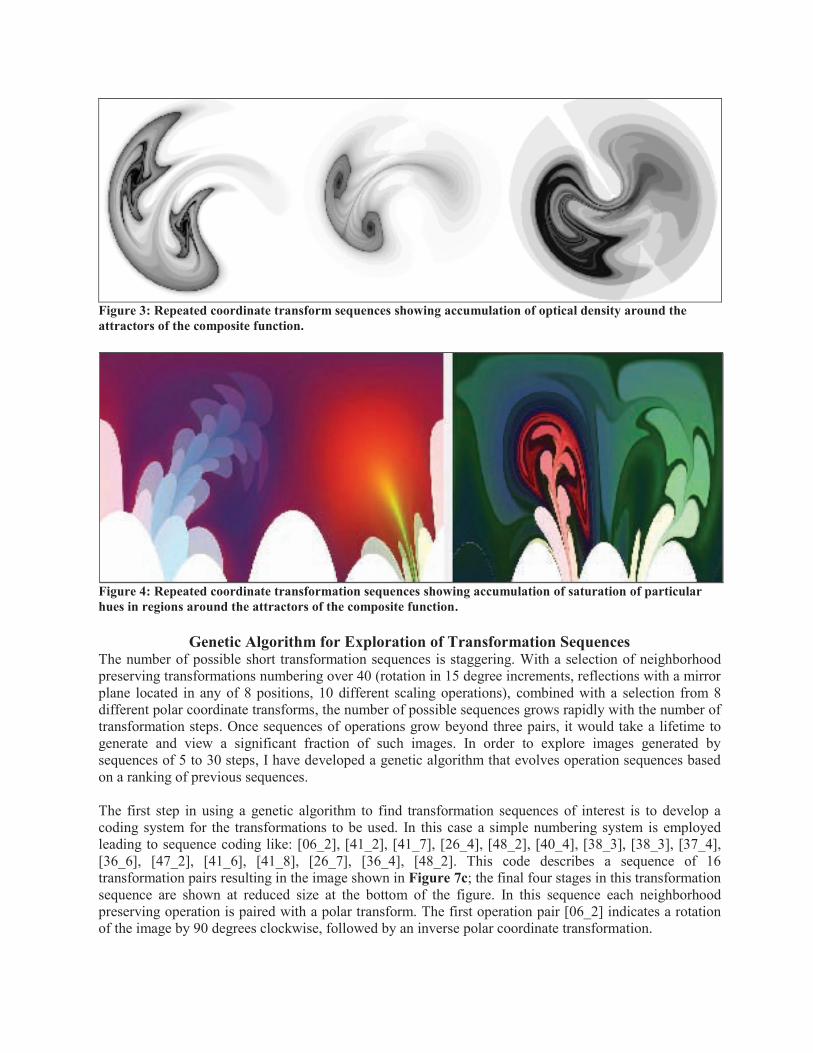
Figure 3: Repeated coordinate transform sequences showing accumulation of optical density around the attractors of the composite function.

Figure 4: Repeated coordinate transformation sequences showing accumulation of saturation of particular hues in regions around the attractors of the composite function.

Genetic Algorithm for Exploration of Transformation Sequences The number of possible short transformation sequences is staggering. With a selection of neighborhood preserving transformations numbering over 40 (rotation in 15 degree increments, reflections with a mirror plane located in any of 8 positions, 10 different scaling operations), combined with a selection from 8 different polar coordinate transforms, the number of possible sequences grows rapidly with the number of transformation steps. Once sequences of operations grow beyond three pairs, it would take a lifetime to generate and view a significant fraction of such images. In order to explore images generated by sequences of 5 to 30 steps, I have developed a genetic algorithm that evolves operation sequences based on a ranking of previous sequences. The first step in using a genetic algorithm to find transformation sequences of interest is to develop a coding system for the transformations to be used. In this case a simple numbering system is employed leading to sequence coding like: [06_2], [41_2], [41_7], [26_4], [48_2], [40_4], [38_3], [38_3], [37_4], [36_6], [47_2], [41_6], [41_8], [26_7], [36_4], [48_2]. This code describes a sequence of 16 transformation pairs resulting in the image shown in Figure 7c; the final four stages in this transformation sequence are shown at reduced size at the bottom of the figure. In this sequence each neighborhood preserving operation is paired with a polar transform. The first operation pair [06_2] indicates a rotation of the image by 90 degrees clockwise, followed by an inverse polar coordinate transformation.

The second requirement for using a genetic algorithm is to develop a fitness function that can influence the level of participation of each code in the population of the next generation of sequences. To assign the reproductive fitness to each individual sequence I have simply looked at each image from a generation of sequences and assigned a score based on my evaluation of its aesthetic quality or novelty. These scores are used in the recombination process to bias the population of parent sequences.

Figure 5: The largest image is the product of recombination of the sequences that generate the two images in the column to its left. Each of these in turn is the product of the parent images to its left and so on. 5a {[06_1], [18_3], [30_1], [18_1], [19_2]}; 5b {[27_2], [03_2], [33_4], [34_1], [18_1], [19_2]}.

Finally, the genetic algorithm selects pairs of sequences from the parent generation to create offspring. It uses the first part of the sequence of the first parent in combination with the second part of the sequence of the second parent to generate a new child sequence. Most commonly the crossover point, where the child sequence switches from using operations from the first parent to operations from the second, occurs after half the child sequence's operations have been determined, but this can also be adjusted based on the fitness of each parent. An additional important factor in the genetic algorithm used to generate these sequences is the incorporation of the ideas of mutation and drift. Mutation results in the arbitrary and random replacement of one operation in a child sequence with a randomly chosen alternative operation. Typically, I have used a mutation rate of around 0.1% (i.e. one time in 1000 rather than using the operation indicated by the appropriate parent sequence, the child uses a randomly chosen operation). Drift

results in the exchange of one operation for one with closely related properties. A certain percentage of the time, when an operation with a continuous range of values (e.g. rotation by x) is called for by the parent sequence, the child sequence will instead employ a close variant (e.g. rotation by x+15 degrees). Figure 5 shows two images illustrating the evolution of sequences using this genetic algorithm.

Observations Having created, reviewed, triaged and prioritized many images created using the methods described above over a period of several years, there are a number of features that I still find particularly compelling about them. The black region in all these images (for example, Figures 7 and 8 below) is the result of numerous relatively simple transformations of the initial square, and all colored regions were originally from the border around its outside edge. Many of the most interesting and organic looking images have an inverse polar coordinate

Figure 6: Eleven pairs of transformations with rainbow overlays produce this image.

transform as the final step, unrolling complex geometry into a shape easily perceived as a landscape or portrait. Close examination of many of these images reveals bent and distorted lines of symmetry. In Figure 6 the large, arch shaped, red bounded region can be seen to contain roughly the same elements present in the region outside the red lines. This region can in turn be seen to be composed of two nearly equivalent portions (divided along the inner red line). This repeated occurrence of near symmetry is inherent in the operations used to construct these images, and lends a pleasing internal consistency to many of the images.

Figure 7 (a-d): A selection of the forms that can be generated using serial coordinate transformations. Along the bottom of 7c and 7d are shown the four final precursor images in the transformation sequence leading to the large image.

Figures 7 and 8 show a sampling of the variety of forms that can be created using the method described here. Many form families have been found, each exhibiting nearly endless variation as early operations in long sequences are changed, or as continuous parameters are varied. To date some of the most prevalent forms (either because I have selected for them in the evolutionary process, or because they are common solutions to the

convoluted functions being generated) have been the bird (as in Figure 7c), the dancers (Figure 8a), the lander (Figure 7d) and the flower (Figure 7b). Doubtless, many more forms exist, as I have only viewed ~250,000 images created using this method, which represent only a tiny sliver of the universe of serial coordinate transform images.

Figure 8: Serial transform sequences with (a) special effects or (b) cropped regions of interest.

References

[1] Bleicher, L. S., Serial Polar Transformations Of Simple Geometries. Presentation to the 2004 ISAMA meeting, Chicago, Il. http://www.mi.sanu.ac.rs/vismath/bleeicher/index.html [2] Krawczyk, R. J., Curving Spirolaterals. Mathematics & Design 2001 Conference, Geelong, Australia, July, 2001 http://mypages.iit.edu/~krawczyk/md01.pdf [3] Dehlinger, H. E., The Artist´s Intentions and Genetic Coding in Algorithmically Generated Drawings. Generative Art 1998. http://www.generativeart.com/on/cic/ga98/book/4.pdf For more related images see http://Porterbleicher.g2gm.net/computed-paintings For animations in 2D and 3D see http://www.youtube.com/user/solporter?feature=mhum

EvaÊ Hild:Ê Large-scaleÊ SculpturesÊ

NatÊ FriedmanÊ[email protected]Ê

ÊIntroductionÊÊThis paper presents Swedish Sculptor Eva Hild’s recent large-scale sculptures. In previous articles we have discussed Eva Hild’s ceramic sculptures [1] as well as her recent snow sculpture [2], which was also a large-scale sculpture. Here we will consider her three commissioned large-scale outdoor sculptures Hollow, 2006, Patined bronze, Campus Varberg, Sweden; Whole,2007, White-painted bronze, Cheong-ju, South Korea; and Wholly, 2010, Aluminum, Boras, Sweden. In these works, Hild shows that her unique form style and technique is equally impressive in the large- scale. Eva Hild’s sculptures are beautifully shaped surfaces that enclose rounded spaces. Light can then caress the surfaces and fill the spaces. I consider Hollow,Ê Whole,Ê andÊ Wholly to be among the best of large-scale contemporary sculpture.

HollowÊThe first monumental sculpture Hollow is shown in Figure 1. This figure shows view Hollow with Eva Hild reclining in her first large-scale finished sculpture before installation in the final site. Space was introduced into form in the 20th century by such sculptors as Barbara Hepworth and Henry Moore. Here Hild

takes form and space to a new level. As in all of Hild’s sculptures, it is interesting from all directions, as also evidenced by the alternate views in Figures 1 and 2. Being a small child allows one to really experience Eva Hild’s large-scale sculptures. As in her ceramic sculpture, the range of light effects is also impressive.

FigureÊ 1.Ê Hollow, with Eva Hild reclining. Ê

convoluted functions being generated) have been the bird (as in Figure 7c), the dancers (Figure 8a), the lander (Figure 7d) and the flower (Figure 7b). Doubtless, many more forms exist, as I have only viewed ~250,000 images created using this method, which represent only a tiny sliver of the universe of serial coordinate transform images.

Figure 8: Serial transform sequences with (a) special effects or (b) cropped regions of interest.

References

[1] Bleicher, L. S., Serial Polar Transformations Of Simple Geometries. Presentation to the 2004 ISAMA meeting, Chicago, Il. http://www.mi.sanu.ac.rs/vismath/bleeicher/index.html [2] Krawczyk, R. J., Curving Spirolaterals. Mathematics & Design 2001 Conference, Geelong, Australia, July, 2001 http://mypages.iit.edu/~krawczyk/md01.pdf [3] Dehlinger, H. E., The Artist´s Intentions and Genetic Coding in Algorithmically Generated Drawings. Generative Art 1998. http://www.generativeart.com/on/cic/ga98/book/4.pdf For more related images see http://Porterbleicher.g2gm.net/computed-paintings For animations in 2D and 3D see http://www.youtube.com/user/solporter?feature=mhum

EvaÊ Hild:Ê Large-scale Sculptures

NatÊ [email protected]

Figure 1. Hollow, 2006, Patined bronze, 250 mx 175 cm, Campus Varberg, Sweden. Figure 2. Hollow, alternate view.

Whole The second monumental sculpture Whole is shown in Figure 4 in the initial carving stage as a styrofoam sculpture (Eva Hild on the right), from which a mold was made for the bronze casting in Figure 5. The final sculpture is shown in Figure 6. An alternate view is shown in Figure 7, where the outdoor setting allows for wonderful night lighting.

Figure 5. Bronze cast of Whole. Figure 6. Whole, 2007, White-painted bronze, 280 x 250 cm, Cheong-ju, South Korea. Figure 7. Whole, view with night lighting.

Figure 4. Whole, styrofoam stage.

Figure 1. Hollow, 2006, Patined bronze, 250 mx 175 cm, Campus Varberg, Sweden. Figure 2. Hollow, alternate view.

Whole The second monumental sculpture Whole is shown in Figure 4 in the initial carving stage as a styrofoam sculpture (Eva Hild on the right), from which a mold was made for the bronze casting in Figure 5. The final sculpture is shown in Figure 6. An alternate view is shown in Figure 7, where the outdoor setting allows for wonderful night lighting.

Figure 5. Bronze cast of Whole. Figure 6. Whole, 2007, White-painted bronze, 280 x 250 cm, Cheong-ju, South Korea. Figure 7. Whole, view with night lighting.

Figure 4. Whole, styrofoam stage.

Wholly The third large-scale sculpture is Wholly, shown in Figure 8, with Eva Hild. This is the largest of the three sculptures. It is a monumental abstract reclining form. Here in sunlight, the interaction with form and space is enhanced. Alternate views are shown in Figures 9-11.The change in direction of outdoor sunlight during the day results in constantly changing light effects so that images of the sculpture are constantly changing. In particular, note the light and shadow contrast and shapes in Figures 10 and 11.

Figure 8. Wholly with Eva Hild, 2010, Aluminum, 200 x 400 cm, Boras, Sweden. Conclusion Eva Hild’s works Hollow, Whole, and Wholly are truly great examples of sculpture as a combination of form, space, and light. We can only look forward to her future such works. For additional discussion of her works, see [3] as well as her website evahild.com. We thank Eva Hill for permission to use the images from her website.

Figure 9. Wholly, alternate view. Figure 10. Wholly, another alternated view.

Figure 11. Wholly, alternate view. Figure 12. Wholly, view with night lighting.

References

[1] Nat Friedman, Eva Hild: Sculpture and Light, Hyperseeing, August, 2007, www.isama.org/hyperseeing/. [2] Eva Hild, Dan Schwalbe, Richard Seeley, Beth-Hassinger Seeley, and Stan Wagon, Eva Hild’s Perpetual Motion In Snow, Hyperseeing, Spring, 2011, www.isama.org/hyperseeing/. [3] Eva Hild, 2009, text: Love Jonsson and Peter Eklund, Carlsson Bokforlag, Stockholm.

Recent 3D Printed Sculptures

Henry Segerman

1 Introduction

I am a mathematician and a mathematical artist, currently a research fellow in the Department of Mathemat-ics and Statistics at the University of Melbourne, Australia. My mathematical research is in 3-dimensionalgeometry and topology, and concepts from those areas often appear in my work. Other artistic interestsinvolve procedural generation, self reference, ambigrams and puzzles.

All of the sculptures in this article were fabricated by the 3D printing service Shapeways. The materialused is nylon plastic (PA 2200, Selective-Laser-Sintered) for all of the sculptures apart from “Knotted Cog”,which is made from stainless steel infused with bronze. I design my sculptures in Rhinoceros, which isa NURBS based modelling tool, often using the python scripting interface. In designing sculptures usingscripting and then producing them using 3D printing, it is possible to get very close to mathematically pre-cise geometry, which is often difficult to achieve by other means.

Sections 2, 3 and 4 of this article are on the themes of fractal graphs, surfaces native to the 3-dimensionalsphere, and 4-dimensional polytopes. Finally, section 5 is a miscellany of other designs.

2 Fractal graphs

These are part of a series of sculptures exploring graphs embedded in R3 with a fractal structure analogous tothat found in constructions of space filling curves. Starting from a simple initial graph, we repeatedly apply asubstitution move. The substitution move replaces each vertex of the graph from step i with a small graph instep i+1, and it replaces each edge of the graph from step i with some number of parallel edges connectingthe small graphs in step i+ 1 corresponding to the endpoints of the vertices in step i. This construction isexplored in detail in [1].

Octahedron Fractal Graph This is a graph embedded in R3 as a subset of an “octahedral lattice”,which is related to the tessellation of space using octahedra and tetrahedra. See Figure 1b for the constructionrule: Each vertex at each step of the construction is degree 4, and is replaced at the next step by a smalloctahedron. For each edge at the previous step (shown in blue) we remove the two red edges that intersect it,and add in the two green edges parallel to it. We begin the construction with the first step being the edges ofan octahedron. After the first substitution, we get an outer shell around a small octahedron. We discard thissmall octahedron (otherwise the object would not be connected) and continue. This is the result at the fourthstep.

Fractal Graph 3 This is a graph embedded in 3-dimensional space as a subset of the cubic lattice (seeFigure 1c). Each vertex at each step of the construction is degree 3, and has the incident edges arrangedeither in a ‘T’ formation, or like a corner of a cube. The vertex is replaced at the next step by a subgraph ofa 3 × 3 × 3 cubical grid, the choice determined by whether the edges meeting at the vertex are in the ‘T’ or‘corner’ shape. Each edge is replaced at the next step by four parallel edges, joining to the midpoints of thesides of each 3 × 3 face of the 3 × 3 × 3 cubical grid. We begin the construction with the first step beingthree edges meeting in a corner formation, and this is the result at the fourth step.

1

(a) Octahedron FractalGraph sculpture.

(b) The substitution move. (c) Fractal Graph: A viewfrom ‘outside the corner’.

(d) Reverse view.

Figure 1: Octahedron Fractal Graph, 2010, 10.3×10.3×10.3 cm. and Fractal Graph 3, 2011, 10.6×10.6×10.6 cm.

3 Surfaces in S3

These designs are based on various parametric surfaces, given by trigonometric functions in the 3-sphere, S3,viewed as the set of points at distance 1 from the origin in R4. We use stereographic projection from S3 toR3 to get an object that can be printed in our universe. When the surface goes through the point from whichwe stereographically project, the image would go off to infinity in R3. To save on costs, I have removed theparts that would require an infinite amount of plastic to print.

Hopf fibration The surface here is a torus (in fact, the image of a Clifford torus in S3), with a diskremoved around infinity. Although it is possible to choose a projection that does not go through infinity, theresult wouldn’t have the same symmetries in R3. In particular, the torus cuts R3 into two pieces, and thesecan only be congruent if the torus goes through infinity. I came to this design through trying to representthe Hopf fibration. The Hopf fibration describes S3 as being a union of fibres, each fibre being a circle, andwith one fibre for each point of the 2-sphere. Each of the corner curves of the square cross-section tubes isa circular fibre of the fibration. The pair of tubes going in the transverse direction to all of the others comefrom the mirror image fibration, and are necessary to keep the sculpture connected.

(a) Hopf Fibration: A 2-fold symmetry axis.

(b) A generic viewpoint. (c) Round Möbius Strip: Ageneric viewpoint.

(d) A 2-fold symmetry axis.

Figure 2: Hopf Fibration, 2010, 10.8×10.8×3.4 cm and Round Möbius Strip, 2011, 15.2×10.9×6.2 cm.

Round Möbius Strip The usual version of a Möbius strip has as its single boundary curve an unknottedloop. This unknotted loop can be deformed into a round circle, with the strip deformed along with it. Thisshows one possible way to do this (sometimes called the “Sudanese Möbius strip”). The boundary of the stripis the circle in the middle. The other boundary of the design is the cut out around infinity, so strictly speakingthis is a punctured Sudanese Möbius strip. Again, the choice of a projection that goes through infinity makes

(a) Octahedron FractalGraph sculpture.

(b) The substitution move. (c) Fractal Graph: A viewfrom ‘outside the corner’.

(d) Reverse view.

Figure 1: Octahedron Fractal Graph, 2010, 10.3×10.3×10.3 cm. and Fractal Graph 3, 2011, 10.6×10.6×10.6 cm.

3 Surfaces in S3

These designs are based on various parametric surfaces, given by trigonometric functions in the 3-sphere, S3,viewed as the set of points at distance 1 from the origin in R4. We use stereographic projection from S3 toR3 to get an object that can be printed in our universe. When the surface goes through the point from whichwe stereographically project, the image would go off to infinity in R3. To save on costs, I have removed theparts that would require an infinite amount of plastic to print.

Hopf fibration The surface here is a torus (in fact, the image of a Clifford torus in S3), with a diskremoved around infinity. Although it is possible to choose a projection that does not go through infinity, theresult wouldn’t have the same symmetries in R3. In particular, the torus cuts R3 into two pieces, and thesecan only be congruent if the torus goes through infinity. I came to this design through trying to representthe Hopf fibration. The Hopf fibration describes S3 as being a union of fibres, each fibre being a circle, andwith one fibre for each point of the 2-sphere. Each of the corner curves of the square cross-section tubes isa circular fibre of the fibration. The pair of tubes going in the transverse direction to all of the others comefrom the mirror image fibration, and are necessary to keep the sculpture connected.

(a) Hopf Fibration: A 2-fold symmetry axis.

(b) A generic viewpoint. (c) Round Möbius Strip: Ageneric viewpoint.

(d) A 2-fold symmetry axis.

Figure 2: Hopf Fibration, 2010, 10.8×10.8×3.4 cm and Round Möbius Strip, 2011, 15.2×10.9×6.2 cm.

Round Möbius Strip The usual version of a Möbius strip has as its single boundary curve an unknottedloop. This unknotted loop can be deformed into a round circle, with the strip deformed along with it. Thisshows one possible way to do this (sometimes called the “Sudanese Möbius strip”). The boundary of the stripis the circle in the middle. The other boundary of the design is the cut out around infinity, so strictly speakingthis is a punctured Sudanese Möbius strip. Again, the choice of a projection that goes through infinity makes

the sculpture particularly symmetric. This was designed with the assistance of Saul Schleimer, who is amathematician at the University of Warwick.

Round Klein Bottle This is made by gluing two copies of the Round Möbius Strip along their bound-aries, and so this is actually a doubly punctured Klein bottle. A Klein bottle in 3-dimensional space mustintersect itself, and in this case it intersects along a straight line.

(a) A generic view-point.

(b) The 4-fold sym-metry axis.

(c) One of the 2-fold sym-metry axes.

(d) The other 2-fold symme-try axis.

Figure 3: Round Klein Bottle, 2011, 15.2×15.2×10.9 cm.

Knotted cog The parametrization used here would make a Möbius strip with 3 half-twists, if the cog teethon the inside linked up across the gap. Instead, the design is a trefoil knot, with near-meshing cogs. In orderfor the teeth to mesh rather than collide, there has to be an odd number of teeth around the strip, and in orderto preserve the 3-fold symmetry, the number must also be a multiple of three. This restricted the possibilitiesto the extent that it was easy to choose 33 on aesthetic grounds (See Figure 6a).

4 4-dimensional polytopes

These are representations of the edges of regular 4-dimensional polytopes, also known as polychora. Justas 3-dimensional polyhedra are named for the number of 2-dimensional faces they have, the 4-dimensionalpolychora are named for the number of 3-dimensional cells they have. The polytopes are native to R4, butcan be radially projected onto the unit S3 in R4, where we fatten the edges into tubes of constant radius.From here, we stereographically project to R3 to produce our sculptures, as with the surfaces in S3.

24-Cell This is the 24-cell, which has 24 octahedral cells. The point from which we stereographicallyproject is at the centre of one of the octahedra, so the edges do not pass through infinity, and we need not cutout a region to get a finite sculpture.

(a) A generic viewpoint. (b) A 2-fold symmetry axis. (c) A 3-fold symmetry axis. (d) A 4-fold symmetry axis.

Figure 4: 24-Cell, 2011, 9.0×9.0×9.0 cm.

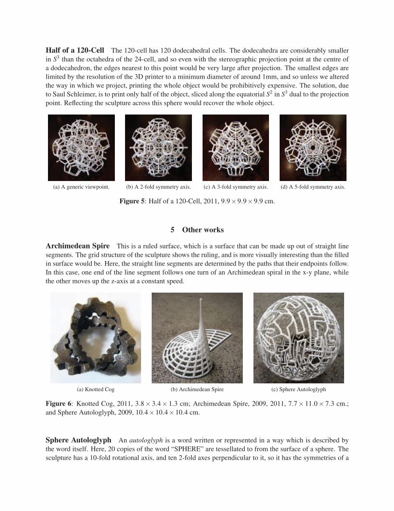
Half of a 120-Cell The 120-cell has 120 dodecahedral cells. The dodecahedra are considerably smallerin S3 than the octahedra of the 24-cell, and so even with the stereographic projection point at the centre ofa dodecahedron, the edges nearest to this point would be very large after projection. The smallest edges arelimited by the resolution of the 3D printer to a minimum diameter of around 1mm, and so unless we alteredthe way in which we project, printing the whole object would be prohibitively expensive. The solution, dueto Saul Schleimer, is to print only half of the object, sliced along the equatorial S2 in S3 dual to the projectionpoint. Reflecting the sculpture across this sphere would recover the whole object.

(a) A generic viewpoint. (b) A 2-fold symmetry axis. (c) A 3-fold symmetry axis. (d) A 5-fold symmetry axis.

Figure 5: Half of a 120-Cell, 2011, 9.9×9.9×9.9 cm.

5 Other works

Archimedean Spire This is a ruled surface, which is a surface that can be made up out of straight linesegments. The grid structure of the sculpture shows the ruling, and is more visually interesting than the filledin surface would be. Here, the straight line segments are determined by the paths that their endpoints follow.In this case, one end of the line segment follows one turn of an Archimedean spiral in the x-y plane, whilethe other moves up the z-axis at a constant speed.

(a) Knotted Cog (b) Archimedean Spire (c) Sphere Autologlyph

Figure 6: Knotted Cog, 2011, 3.8× 3.4× 1.3 cm; Archimedean Spire, 2009, 2011, 7.7× 11.0× 7.3 cm.;and Sphere Autologlyph, 2009, 10.4×10.4×10.4 cm.

Sphere Autologlyph An autologlyph is a word written or represented in a way which is described bythe word itself. Here, 20 copies of the word “SPHERE” are tessellated to from the surface of a sphere. Thesculpture has a 10-fold rotational axis, and ten 2-fold axes perpendicular to it, so it has the symmetries of a

regular 10-gon. The form of the sculpture is in some ways forced by the limits of technology: If it had beeneasy to (2-dimensionally) print onto the surface of a sphere, then I would have done so, and presumably adesign like that could be realised using the machinery that makes geographic globes. Within the mediumof 3D printing, one could print a solid sphere, with grooves or ridges used to form the letters. This wouldbe very expensive however. Drawing the letters as a network of tubes solves this problem, although it doesmean that the holes in the “P” and “R” have to be inferred.

Juggling Club Motion This shows (a somewhat idealized version of) the path of a juggling club as itis thrown from the right hand to the left, making a single spin. The club is shown in a “multiple exposure”style as it follows a parabolic path while rotating at constant speed.

(a) A view from behind the juggler. (b) A view from the side. (c) A view from in front of the juggler.

Figure 7: Juggling Club Motion, 2011, 4.5×4.1×6.1 cm.

References

[1] Henry Segerman, Fractal graphs by iterated substitution, Journal of Mathematics and the Arts,c©Taylor and Francis, Volume 5, Issue 2, 2011, pp. 51–70.

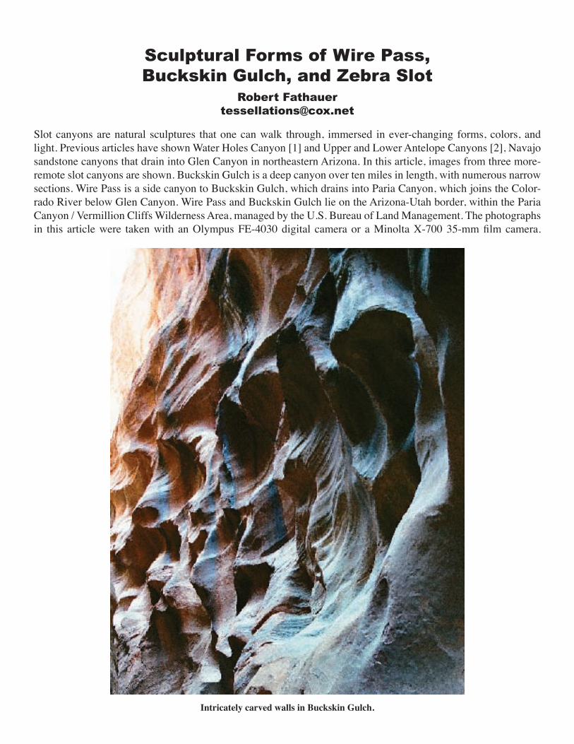
Slot canyons are natural sculptures that one can walk through, immersed in ever-changing forms, colors, and light. Previous articles have shown Water Holes Canyon [1] and Upper and Lower Antelope Canyons [2], Navajo sandstone canyons that drain into Glen Canyon in northeastern Arizona. In this article, images from three more-remote slot canyons are shown. Buckskin Gulch is a deep canyon over ten miles in length, with numerous narrow sections. Wire Pass is a side canyon to Buckskin Gulch, which drains into Paria Canyon, which joins the Color-rado River below Glen Canyon. Wire Pass and Buckskin Gulch lie on the Arizona-Utah border, within the Paria Canyon / Vermillion Cliffs Wilderness Area, managed by the U.S. Bureau of Land Management. The photographs in this article were taken with an Olympus FE-4030 digital camera or a Minolta X-700 35-mm film camera.

Intricately carved walls in Buckskin Gulch.

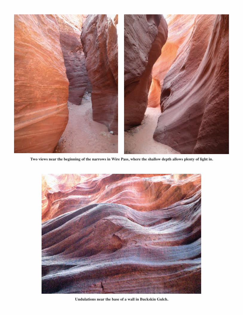
Two views near the beginning of the narrows in Wire Pass, where the shallow depth allows plenty of light in.

Undulations near the base of a wall in Buckskin Gulch.

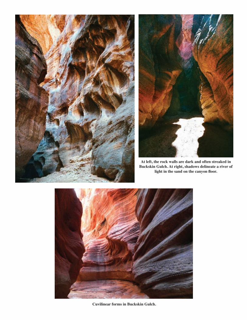
Cuvilinear forms in Buckskin Gulch.

At left, the rock walls are dark and often streaked in Buckskin Gulch. At right, shadows delineate a river of

light in the sand on the canyon floor.

Cuvilinear forms in Buckskin Gulch.

At left, the rock walls are dark and often streaked in Buckskin Gulch. At right, shadows delineate a river of

light in the sand on the canyon floor.

Two more views of Buckskin Gulch.

One of many pools that must be waded through when hiking Buckskin Gulch. This one is around 3’ deep.

Zebra Slot is a short side canyon to Harris Wash, a tributary of the Escalante River, which in turn joins the Colorado above Lake Powell. It is located at the eastern edge of Grand Staircase - Escalan-te National Monument. Zebra Slot gets its name from the dark-and-light banded sandstone in its up-per reaches. This is a very narrow slot, in sections necking down at the bottom to less than a shoe’s width.

Zebra Slot is named for its unique banded sandstone.

Zebra Slot is a short side canyon to Harris Wash, a tributary of the Escalante River, which in turn joins the Colorado above Lake Powell. It is located at the eastern edge of Grand Staircase - Escalan-te National Monument. Zebra Slot gets its name from the dark-and-light banded sandstone in its up-per reaches. This is a very narrow slot, in sections necking down at the bottom to less than a shoe’s width.

Zebra Slot is named for its unique banded sandstone.

Soft undulations in the lower portion of the canyon, where the striping in the sandstone coloration is not present.

Complex surfaces and striping create visual interest in this image. The different colors in different areas of these photo-graphs is primarily due to effects of the lighting rather than

the inherent differences in the stone.

The features in the walls that look like pock marks are iron oxide concretions known as “moqui marbles” .

References

[1] Robert Fathauer and Nat Friedman, Water Holes Canyon: Form, Space, Light, and Color,Hyperseeing, March/April 2008, www.isama.org/hyperseeing/. [2] Robert Fathauer and Nat Friedman, Slot Canyons: Form, Space, Light, Color, Hyperseeing, April/June 2009, www.isama.org/hyperseeing/.

Two views of the same narrow passage, looking upstream (left) and downstream (right). Note the marked assymetry in the curves of the sandstone fins.

Schematic of the approximate shape of the walls roughly midway up the photographs above, where the arrow indicates the direction of water flow. The structure is roughly periodic, and the two sides are approximately 180° out of phase.




June 18-22, 2012

General Information Organizers ISAMA 2012 will be held June 18-22, 2012 at DePaul University co-organized with Steve Luecking and the Illinois Institute of Technology (IIT), co-organized with Robert Krawczyk. ISAMA 2012 celebrates the 20th anniversary of the first Art and Mathematics Conference AM92, organized by Nat Friedman at the University at Albany, New York in June, 1992.

Conference Plans

Talks will be scheduled for June 18-20, excursions June 21 and teacher workshops June 22.

Call for papers

Papers are due March 15, 2012. Papers should be sent to Nat Friedman at [email protected] .

The format for papers is the same as for ISAMA 2011 and can be seen at www.hyperseeing.org/hyperseeing/ in the Summer, 2011 issue, which is the Proceedings of ISAMA 2011. This is the same as the Bridges format.

Registration Fees

The registration fee will be $200 and will include a copy of the Proceedings and excursion costs. Refreshments will also be provided during the talks and workshops. Details for payment are in the registration form at www.isama.org

Invited Speakers

Invited speakers will include Robert Bosch, Gabrielle Meyer, Jeanne Gang and Mark Schendel from Studio Gang Architects. Jeanne Gang won a 2011 Mac Arthur Fellowship. Jeanne and Mark are married and the two principal partners of Studio Gang Architects. Mark also spoke at ISAMA 2011.




June 18-22, 2012


Conference Plans


Call for papers



Registration Fees


Invited Speakers





June 18-22, 2012


Conference Plans


Call for papers



Registration Fees


Invited Speakers


Keizo Ushio: Sculpture

The Japanese stone carver Keizo Ushio will be carving a granite sculpture outdoors at DePaul University during June, 2012 and plans to finish the sculpture during the conference. Keizo also carved a sculpture during June, 1999 at the first ISAMA conference held at the University of the Basque Country in San Sebastian, Spain, co-organized with Javier Barrallo. We are also hoping to exhibit four of Keizo’s large sculptures, currently on view in Stockholm, Sweden, on the IIT campus.

Hotels to follow.

Inquiries: [email protected]

Keizo Ushio, Oushi Zokei 2007, Blue granite, 160 x 240 x 160 cm, Joyama Park, Nagano City, Japan, Winner of 2007 Nagano City Open Air

Sculpture Prize

ISAMAwww.isama.org

BECOME A MEMBER

The International Society of the Arts, Mathematics, and Architecture

ISAMA Membership Registration

Membership in ISAMA is free. Membership implies you will receive all ISAMA email announcements concerning conferences and other news items of interest.

Name………………………………………………………………………………………………………………….

Address……………………………………………………………………………………………………………………………………………………………………………………………………………………………………………………………………………………………………………………………………………………………………………………………………………………………………………………………………………………………………………………………………………………………………………………………………………………………………………………………………………………………………………………………………………………………

Email address…………………………………………………………………………………………………………………………….

Interests…………………………………………………………………………………………………………………………………………………………………………………………………………………………………………………………………………………………………………………………………………………………………………………………………………………………………………………………………………………………………………………………………………………………………………………………………………………………………………………………………………………………………………………………………………………………………………………………………………………………………………………………………………………………………………………

Please email completed form to Nat Friedman at [email protected]

BECOME A MEMBER




June 18-22, 2012


HYPERSEEING - ISAMA Homepage · For inclusion in Hyperseeing, au-thors are invited to email...

Documents

Transcript of HYPERSEEING - ISAMA Homepage · For inclusion in Hyperseeing, au-thors are invited to email...