Hydrological assessment and analysis of Neales-Peake Catchment · Hydrological assessment and...

Hydrological assessment and analysis of the Neales-Peake Catchment

DEWNR Technical note 2014/16

Hydrological assessment and analysis of the

Neales-Peake Catchment

Mahdi Montazeri and Alex Osti

Department of Environment, Water and Natural Resources

September, 2014

DEWNR Technical note 2014/16

DEWNR Technical note 2014/16 i

Department of Environment, Water and Natural Resources

GPO Box 1047, Adelaide SA 5001

Telephone National (08) 8463 6946

International +61 8 8463 6946

Fax National (08) 8463 6999

International +61 8 8463 6999

Website www.environment.sa.gov.au

Disclaimer

The Department of Environment, Water and Natural Resources and its employees do not warrant or make any representation

regarding the use, or results of the use, of the information contained herein as regards to its correctness, accuracy, reliability,

currency or otherwise. The Department of Environment, Water and Natural Resources and its employees expressly disclaims all

liability or responsibility to any person using the information or advice. Information contained in this document is correct at the

time of writing.

This work is licensed under the Creative Commons Attribution 4.0 International License.

To view a copy of this license, visit http://creativecommons.org/licenses/by/4.0/.

© Crown in right of the State of South Australia, through the Department of Environment, Water and Natural Resources 2014

ISBN 978-1-922255-12-9

Preferred way to cite this publication

Montazeri, M. and Osti, A., 2014, Hydrological assessment and analysis of Neales-Peake Catchment, DEWNR Technical note

2014/16, Government of South Australia, through Department of Environment, Water and Natural Resources, Adelaide

http://creativecommons.org/licenses/by/4.0/

DEWNR Technical note 2014/16 ii

Acknowledgements

The authors would like to acknowledge all who have helped with this project.

We thank Justin Costelloe from the University of Melbourne for his guidance and assistance through all stages of this work. His

depth of knowledge of the hydrology of the Lake Eyre Basin, shared with us through time spent in the field, as a sounding board

for ideas during model development and provided through review of this report have made this work possible. We also thank

Pete Richards for his unique insights provided to us around some truly spectacular locations.

We also thank Mark Alcorn and Matt Gibbs (both of DEWNR) for their guidance and advice in model development and Kumar

Savadamuthu (DEWNR) for his ongoing assistance and review of this report.

Funding for these projects has been provided by the Australian Government through the Department of the Environment,

Office of Water Science. See www.bioregionalassessments.gov.au for further information.

DEWNR Technical note 2014/16 iii

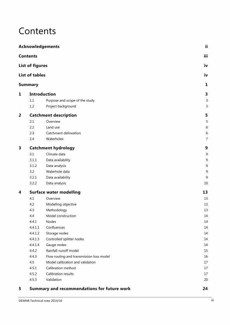
Contents

Acknowledgements ii

Contents iii

List of figures iv

List of tables iv

Summary 1

1 Introduction 3

1.1 Purpose and scope of the study 3

1.2 Project background 3

2 Catchment description 5

2.1 Overview 5

2.2 Land use 6

2.3 Catchment delineation 6

2.4 Waterholes 7

3 Catchment hydrology 9

3.1 Climate data 9

3.1.1 Data availability 9

3.1.2 Data analysis 9

3.2 Waterhole data 9

3.2.1 Data availability 9

3.2.2 Data analysis 10

4 Surface water modelling 13

4.1 Overview 13

4.2 Modelling objective 13

4.3 Methodology 13

4.4 Model construction 14

4.4.1 Nodes 14

4.4.1.1 Confluences 14

4.4.1.2 Storage nodes 14

4.4.1.3 Controlled splitter nodes 14

4.4.1.4 Gauge nodes 14

4.4.2 Rainfall-runoff model 15

4.4.3 Flow routing and transmission loss model 16

4.5 Model calibration and validation 17

4.5.1 Calibration method 17

4.5.2 Calibration results 17

4.5.3 Validation 20

5 Summary and recommendations for future work 24

DEWNR Technical note 2014/16 iv

6 References 25

Appendix A: Waterholes bathymetry relationships 26

Appendix B: Calibrated parameters 36

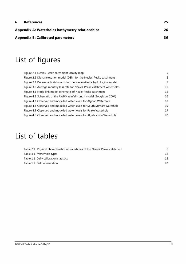
List of figures

Figure 2.1 Neales-Peake catchment locality map 5

Figure 2.2 Digital elevation model (DEM) for the Neales-Peake catchment 6

Figure 2.3 Delineated catchments for the Neales-Peake hydrological model 7

Figure 3.2 Average monthly loss rate for Neales-Peake catchment waterholes 11

Figure 4.1 Node-link model schematic of Neale-Peake catchment 15

Figure 4.2 Schematic of the AWBM rainfall-runoff model (Boughton, 2004) 16

Figure 4.3 Observed and modelled water levels for Afghan Waterhole 18

Figure 4.4 Observed and modelled water levels for South Stewart Waterhole 19

Figure 4.5 Observed and modelled water levels for Peake Waterhole 19

Figure 4.6 Observed and modelled water levels for Algebuckina Waterhole 20

List of tables

Table 2.1 Physical characteristics of waterholes of the Neales-Peake catchment 8

Table 3.1 Waterhole types 12

Table 1.1 Daily calibration statistics 18

Table 1.2 Field observation 20

DEWNR Technical note 2014/16 1

Summary

This technical report describes the methodology and outcomes of a hydrological study undertaken for the Neales-Peake

catchment. The main purpose of this study was to establish a hydrological model for the system to (i) aid in assessing the impacts

on the flow regime if mining operations were to occur within the catchment and (ii) provide a tool that will aid in ecohydrological

assessment of the region.

This study was undertaken by South Australian Department of Environment, Water and Natural Resources’ (DEWNR) Science

Monitoring and Knowledge (SMK) branch as part of the broader Lake Eyre Basin River Monitoring (LEBRM) project, which was

formed to address knowledge gaps pertaining to the potential impacts of coal seam gas and large coal mining projects on the

surface water resources of the Lake Eyre Basin (LEB). The Lake Eyre Basin has been identified as one of the six priority bioregions

where coal seam gas and/or large mining developments are either planned or underway. Along with other partners, DEWNR has

been contracted to address relevant hydro-ecological knowledge gaps within the LEB. The hydrological assessment and analysis

of the Neales-Peake catchment forms part of this work.

The Neales-Peake catchment is an ephemeral, unregulated river system in the far north of South Australia, consisting of the

Neales and Peake Rivers and associated tributaries, with a total catchment area of 34 415 km2. Characterised by complex, multiple

anastomosing channels, shallow channel definition, wide floodplains and waterholes, the ephemeral watercourses of the Neales-

Peake system most commonly flow in response to the more localized thunderstorm-derived rainfall. Such in-channel flow events

occur 1–2 times per year and are important in maintaining aquatic refugia but have limited influence on the connectivity between

waterholes. The volume of the waterholes is often quite small compared with flow in the system and so small runoff events in

the main channel system are capable of filling waterholes to their maximum cease-to-flow level. The larger rainfall events result

in runoff through much of the channel system, recharging the alluvial/floodplain groundwater stores and allowing widespread

migration of aquatic fauna.

The hydrological model used is a catchment model set up in the eWater Source IMS (integrated modelling system) that uses the

Australian Water Balance rainfall/runoff Model (AWBM) to generate runoff for 177 sub-catchments and routes this flow through

the system to discharge at Lake Eyre North, accounting for 20 waterhole storages. Detailed bathymetry of the waterholes in the

system, in addition to observations regarding surface-water/groundwater interactions at the waterholes, was incorporated into

the model, ensuring that waterhole dynamics were accurately represented by the model.

The model was calibrated by comparing modelled stage heights with those heights observed at four key waterholes. The limited

and patchy nature of the data coverage over the study region means that traditional calibration statistics may be misleading.

This being said, the model was able to reproduce observed stage, with an average difference of 6.5% between modelled and

observed median stage height across the waterholes. This translated to an average difference of approximately 9% in average

storage volume. Additionally, it was shown visually that the model tended to replicate the timing of events very well. At each

waterhole the model struggled to identify some smaller flow events, in particular multiple flow events, however it did not register

any false positives and as such was considered fit for purpose.

Although the model is able to reproduce the timing of observed events in the system very well, the model should be considered

limited in its ability to estimate the magnitude of the events. The lack of volumetric information to calibrate the model means

that it is not possible to estimate confidence surrounding simulated discharge volumes.

Recommendations for future work fall into two complementary categories, data collection and model refinement. By conducting

flow gaugings at strategic locations throughout the system a measure of confidence in simulated flow volumes could be gained.

Additionally, more detailed information regarding the surface-water/groundwater interactions at waterholes and throughout the

system would enable a more complete representation of the hydrological dynamics of the catchment. Data that have been

collected are often inconsistent owing to malfunctioning loggers, disturbance from local fauna, theft and varying installation and

removal dates. Establishment of a more permanent monitoring network and the collection of data from such a network would

enable continuous refinement of model parameters and deliver a better understanding of the hydrology of the system.

The Neales-Peake catchment has a varied geography, containing a diverse range of country – from the red sands of the Pedirka

Desert to the hard packed clays of the Gibber Pans. Furthermore, the watercourses of the Neales-Peake are equally varied,

ranging from well-defined incised channels to poorly channelized floodplains. As such, it is unlikely that the rainfall-runoff


response and transmission losses will be consistent throughout the catchment as considered in the model. More comprehensive

data on land type, supplemented by hydrological observations, would allow the calibration of discrete rainfall-runoff and

transmission loss models within subregions of the catchment that share similar geography and hydrology.


1 Introduction

1.1 Purpose and scope of the study

This technical report describes the methodology and outcomes of a hydrological study undertaken for the Neales-Peake

catchment with the main purpose of this study being to:

Establish a hydrological model for the Neales-Peake catchment to (i) aid in assessing the impacts on the flow regime if

mining operations were to occur within the catchment and (ii) provide a tool that will aid in ecohydrological assessment

of the region.

This study was undertaken by DEWNR’s SMK branch as part of the broader Lake Eyre Basin Rivers Monitoring (LEBRM) project,

which was formed to address knowledge gaps pertaining to the potential impacts of coal seam gas and large coal mining projects

on the surface water resources of the Lake Eyre Basin (LEB), informing the Bioregional Assessment Programme. The broad scope

of the study is encompassed by five key objectives:

1. Identify critical surface water sites and their characteristics (e.g. bathymetric relationship) within the study area

2. Disaggregate the study area into physically representative sub-catchments

3. Select appropriate rainfall data; select and calibrate appropriate rainfall-runoff model

4. Select and calibrate appropriate transmission loss function(s)

5. Validate model against observed understanding of system.

1.2 Project background

In responding to perceived uncertainties surrounding the potential water-related impacts associated with the increasing

development in the unconventional petroleum sector in Australia, the Australian Government established the Independent

Expert Scientific Committee (IESC) on Coal Seam Gas and Coal Mining Development. The Independent Expert Scientific

Committee on Coal Seam Gas and Large Coal Mining Development (the IESC) is a statutory body under the Environment

Protection and Biodiversity Conservation Act 1999 (EPBC Act) which provides scientific advice to Australian governments on the

water-related impacts of coal seam gas and large coal mining development proposals.

Under the EPBC Act, the IESC has several legislative functions to:

Provide scientific advice to the Commonwealth Environment Minister and relevant state ministers on the water-

related impacts of proposed coal seam gas or large coal mining developments.

Provide scientific advice to the Commonwealth Environment Minister on:

1. bioregional assessments being undertaken by the Australian Government, and

2. research priorities and projects commissioned by the Commonwealth Environment Minister.

Publish and disseminate scientific information about the impacts of coal seam gas and large coal mining activities on

water resources.

The Lake Eyre Basin has been identified by the IESC as one of the six priority bioregions where coal seam gas and/or large mining

developments are either planned or underway. The Bioregional Assessment Programme is a transparent and accessible

programme of baseline assessments that increase the available science for decision making associated with potential water-

related impacts of coal seam gas and large coal mining developments. A bioregional assessment is a scientific analysis of the

ecology, hydrology, geology and hydrogeology of a bioregion with explicit assessment of the potential direct, indirect and


cumulative impacts of coal seam gas and large coal mining development on water resources. This programme draws on the best

available scientific information and knowledge from many sources, including government, industry and regional communities,

to produce bioregional assessments that are independent, scientifically robust, and relevant and meaningful at a regional scale.

This report is part of a series of studies forming part of the Lake Eyre Basin Rivers Monitoring (LEBRM) Project. LEBRM is one of

three water knowledge projects undertaken by the South Australian Department of Water, Environment and Natural Resources

(DEWNR) to inform the Bioregional Assessment Programme in the Lake Eyre Basin. The three projects are:

Lake Eyre Basin Rivers Monitoring,

Arckaringa and Pedirka Groundwater Assessment and

Lake Eyre Basin Springs Assessment.

The hydrological assessment and analysis of the Neales-Peake catchment forms part of DEWNR’s Lake Eyre Basin River

Monitoring (LEBRM) project. Formed to address knowledge gaps pertaining to the potential impacts of coal seam gas and large

coal mining projects on the surface water resources of the LEB, LEBRM is driven by five key aims, namely to:

Collate and interrogate baseline knowledge regarding the surface waters and water dependent ecosystems of the Lake

Eyre Basin

Identify the locations and attributes of surface water assets, including ecological and cultural values and the attributes

critical for maintaining those values

Collect new hydrological, geomorphic, ecological and cultural knowledge to better inform our understanding of LEB

surface water systems, and to fill gaps in current knowledge

Identify and collate processes and mechanisms through which mining developments may impact upon surface water

resources, assets, attributes and values

Identify surface water assets, attributes and values that are especially vulnerable to the potential impacts of mining

developments.


2 Catchment description

2.1 Overview

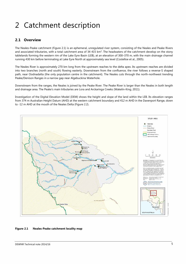
The Neales-Peake catchment (Figure 2.1) is an ephemeral, unregulated river system, consisting of the Neales and Peake Rivers

and associated tributaries, with a total catchment area of 34 415 km2. The headwaters of the catchment develop on the stony

tablelands forming the western rim of the Lake Eyre Basin (LEB), at an elevation of 300–370 m, with the main drainage channel

running 430 km before terminating at Lake Eyre North at approximately sea level (Costelloe et al., 2005).

The Neales River is approximately 270 km long from the upstream reaches to the delta apex. Its upstream reaches are divided

into two branches (north and south) flowing easterly. Downstream from the confluence, the river follows a reverse-S shaped

path, near Oodnadatta (the only population centre in the catchment). The Neales cuts through the north-northwest trending

Peake/Denison Ranges in a narrow gap near Algebuckina Waterhole.

Downstream from the ranges, the Neales is joined by the Peake River. The Peake River is larger than the Neales in both length

and drainage area. The Peake's main tributaries are Lora and Arckaringa Creeks (Wakelin-King, 2011).

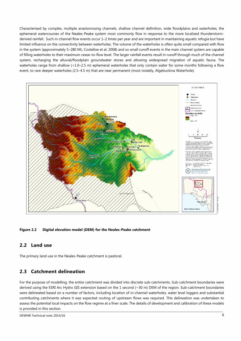
Investigation of the Digital Elevation Model (DEM) shows the height and slope of the land within the LEB. Its elevation ranges

from 374 m Australian Height Datum (AHD) at the western catchment boundary and 412 m AHD in the Davenport Range, down

to -12 m AHD at the mouth of the Neales Delta (Figure 2.2).

Figure 2.1 Neales-Peake catchment locality map


Characterised by complex, multiple anastomosing channels, shallow channel definition, wide floodplains and waterholes, the

ephemeral watercourses of the Neales-Peake system most commonly flow in response to the more localized thunderstorm-

derived rainfall. Such in-channel flow events occur 1–2 times per year and are important in maintaining aquatic refugia but have

limited influence on the connectivity between waterholes. The volume of the waterholes is often quite small compared with flow

in the system (approximately 5–280 ML; Costelloe et al, 2008) and so small runoff events in the main channel system are capable

of filling waterholes to their maximum cease-to-flow level. The larger rainfall events result in runoff through much of the channel

system, recharging the alluvial/floodplain groundwater stores and allowing widespread migration of aquatic fauna. The

waterholes range from shallow (<1.0–2.5 m) ephemeral waterholes that only contain water for some months following a flow

event, to rare deeper waterholes (2.5–4.5 m) that are near permanent (most notably, Algebuckina Waterhole).

Figure 2.2 Digital elevation model (DEM) for the Neales-Peake catchment

2.2 Land use

The primary land use in the Neales-Peake catchment is pastoral.

2.3 Catchment delineation

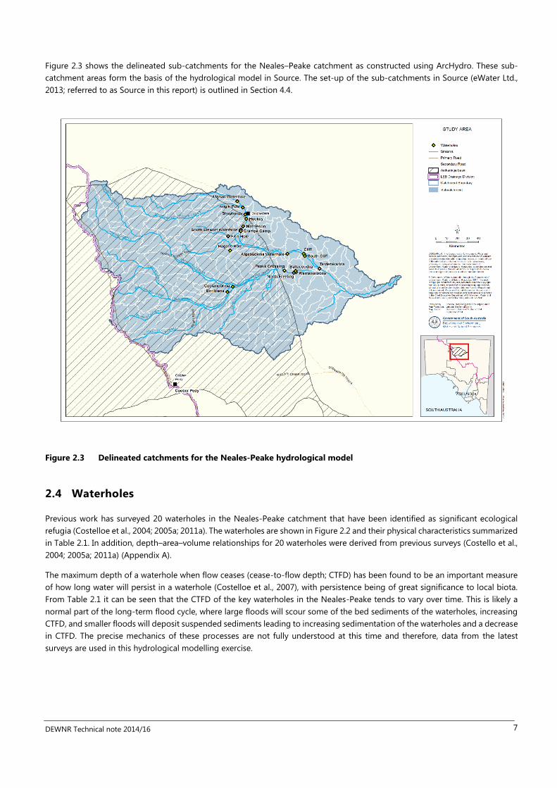
For the purpose of modelling, the entire catchment was divided into discrete sub-catchments. Sub-catchment boundaries were

derived using the ESRI Arc Hydro GIS extension based on the 1 second (~30 m) DEM of the region. Sub-catchment boundaries

were delineated based on a number of factors, including location of in-channel waterholes, water level loggers and substantial

contributing catchments where it was expected routing of upstream flows was required. This delineation was undertaken to

assess the potential local impacts on the flow regime at a finer scale. The details of development and calibration of these models

is provided in this section.


Figure 2.3 shows the delineated sub-catchments for the Neales–Peake catchment as constructed using ArcHydro. These sub-

catchment areas form the basis of the hydrological model in Source. The set-up of the sub-catchments in Source (eWater Ltd.,

2013; referred to as Source in this report) is outlined in Section 4.4.

Figure 2.3 Delineated catchments for the Neales-Peake hydrological model

2.4 Waterholes

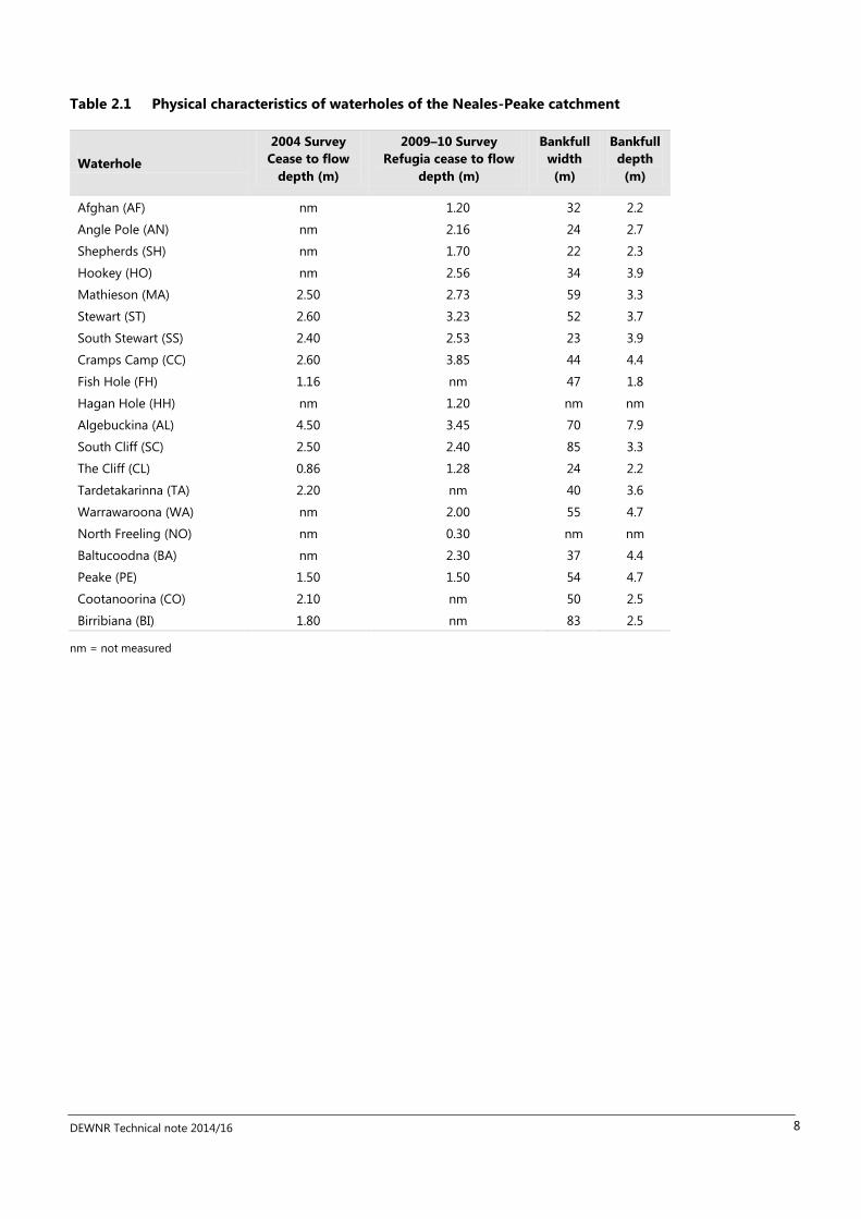
Previous work has surveyed 20 waterholes in the Neales-Peake catchment that have been identified as significant ecological

refugia (Costelloe et al., 2004; 2005a; 2011a). The waterholes are shown in Figure 2.2 and their physical characteristics summarized

in Table 2.1. In addition, depth–area–volume relationships for 20 waterholes were derived from previous surveys (Costello et al.,

2004; 2005a; 2011a) (Appendix A).

The maximum depth of a waterhole when flow ceases (cease-to-flow depth; CTFD) has been found to be an important measure

of how long water will persist in a waterhole (Costelloe et al., 2007), with persistence being of great significance to local biota.

From Table 2.1 it can be seen that the CTFD of the key waterholes in the Neales-Peake tends to vary over time. This is likely a

normal part of the long-term flood cycle, where large floods will scour some of the bed sediments of the waterholes, increasing

CTFD, and smaller floods will deposit suspended sediments leading to increasing sedimentation of the waterholes and a decrease

in CTFD. The precise mechanics of these processes are not fully understood at this time and therefore, data from the latest

surveys are used in this hydrological modelling exercise.


Table 2.1 Physical characteristics of waterholes of the Neales-Peake catchment

Waterhole

2004 Survey

Cease to flow

depth (m)

2009–10 Survey

Refugia cease to flow

depth (m)

Bankfull

width

(m)

Bankfull

depth

(m)

Afghan (AF) nm 1.20 32 2.2

Angle Pole (AN) nm 2.16 24 2.7

Shepherds (SH) nm 1.70 22 2.3

Hookey (HO) nm 2.56 34 3.9

Mathieson (MA) 2.50 2.73 59 3.3

Stewart (ST) 2.60 3.23 52 3.7

South Stewart (SS) 2.40 2.53 23 3.9

Cramps Camp (CC) 2.60 3.85 44 4.4

Fish Hole (FH) 1.16 nm 47 1.8

Hagan Hole (HH) nm 1.20 nm nm

Algebuckina (AL) 4.50 3.45 70 7.9

South Cliff (SC) 2.50 2.40 85 3.3

The Cliff (CL) 0.86 1.28 24 2.2

Tardetakarinna (TA) 2.20 nm 40 3.6

Warrawaroona (WA) nm 2.00 55 4.7

North Freeling (NO) nm 0.30 nm nm

Baltucoodna (BA) nm 2.30 37 4.4

Peake (PE) 1.50 1.50 54 4.7

Cootanoorina (CO) 2.10 nm 50 2.5

Birribiana (BI) 1.80 nm 83 2.5

nm = not measured


3 Catchment hydrology

3.1 Climate data

3.1.1 Data availability

Rainfall data relevant to the study area take the form of either point data (e.g. at gauge locations) or spatially interpolated

products. The sparse rain gauge network across central Australia means that for catchment modelling purposes it is necessary

to use a spatially interpolated rainfall product. In a report produced for DEWNR, Ryu et al. (2014) evaluate four spatially

distributed rainfall products for use in the Neales-Peake catchment. Along with three widely used remotely sensed products

(TRMM, CMORPH and PERSIANN), the authors evaluate data produced through the Australian Water Availability Project (AWAP)

that is interpolated via splines fitted to gauged data. Ryu et al. (2014) determined that TRMM data were the best performing

remotely sensed data both in ability to replicate gauged events and in terms of a rank analysis of rainfall and streamflow stage.

However, AWAP data were found to better replicate observed rainfall totals than all remotely sensed data and were used as the

rainfall data source in this report.

The hydrological modelling of the Neales-Peake also requires potential evapotranspiration (PET) data in order to account for

evaporation and water use from channels and waterholes throughout the catchment. PET data used in this report are Morton’s

Lake PET for the SILO station at Oodnadatta. SILO is an enhanced meteorological data bank providing data for over 4500 Bureau

of Meteorology, BOM, stations around Australia from 1889 to present (Jeffrey et al., 2001). It is hosted by the Queensland

Department of Science, Information Technology, Innovation and the Arts (DSITIA). SILO patched point data are original historical

climate data for a particular BOM station where missing data or aggregated data have been in-filled (or “patched”) using

interpolated values. SILO data are available for Oodnadatta and this is the preferred source of PET data for this project because

it is a consistent and continuous long term PET record which is independently verifiable and defensible.

3.1.2 Data analysis

In order to construct the Neales-Peake catchment model it was necessary for each sub-catchment to have a time series of rainfall

data. These were calculated by considering the overlay of the AWAP grids on the sub-catchments layer and performing an area-

weighted average of the rainfall files for the relevant overlying rainfall cells for each sub-catchment. PET for Oodnadatta was

used for all sub-catchments.

3.2 Waterhole data

3.2.1 Data availability

There are no consistent discharge data available for the Neales-Peake catchment. Opportunistic flow measurements at

Algebuckina Waterhole, have been collected during field trips in periods of flow recession and, in November 2000, a moderate

flow event was observed (Costelloe et al., 2011a). This flood was sub-bankfull but utilised several channels in the anastomosing

channel reach upstream of the waterhole. This enabled the development of a partial rating curve that was used in converting

daily water level data into daily discharge estimates for the period April 2000 – February 2002 (Costelloe et al, 2005a). However,

in that case the rating curve was deemed unreliable above the maximum gauged level (9000ML/d) as larger flows also enter

another channel that bypasses Algebuckina Waterhole. As water level data are a function of channel morphology, this rating

curve cannot be applied to other waterholes for the same time period, or indeed to stage data for Algebuckina Waterhole itself

at a different time owing to the inherent variability of cease-to-flow depths (CTFDs) in the catchment.

Although there are limited flow data, stage data of varying quality and length have been collected for four waterholes over the

period 2000-2013 for the Neales-Peake catchment. Owing to malfunctioning loggers, disturbance from local fauna, theft and

varying installation and removal dates, there is little consistency in data collected across waterholes and no single waterhole has

continuous data for that period (JF Costelloe (University of Melbourne) 2010 pers. comm.), however the data collected are

invaluable and were utilized in this hydrological analysis.


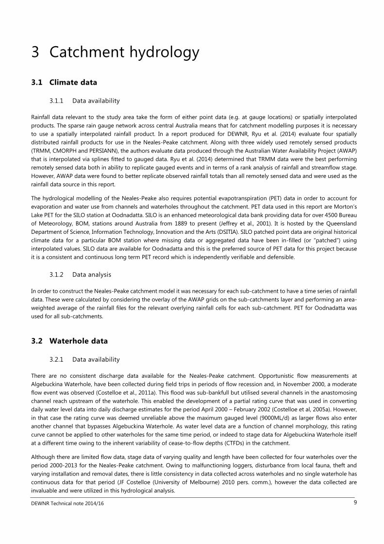
Stage data for Algebuckina Waterhole represent the most complete set of water level data in or nearby the region and are shown

in Figure 3.1. Data shown represent a merging of data collected through multiple loggers installed through the ARIDFLOW project

(Costelloe et al., 2004), Critical Refugia Project (Costelloe, 2011a) and a telemetered gauge installed by DEWNR in 2011, with

post-processing necessary to ensure consistency throughout the period of record (JF Costelloe (University of Melbourne) 2010

pers. comm.).

Figure 3.1 Algebuckina Waterhole stage data

3.2.2 Data analysis

Given the lack of data for the calibration process, flows generated from the model were converted into water levels in waterholes

and compared with observed stage data. To undertake this, a water balance model is required to take the modelled inflows from

a rainfall-runoff model as input and represent the water level in each water hole.

Each storage in the model requires a depth–area–volume relationship to allow the volume in storage to be converted into a

depth (the key variable in the calibration process), as well as an area to allow the net effect of rainfall and evaporation from the

water surface to be taken into account.

Apart from morphological data, loss rates (loss rates are driven by potential evapotranspiration plus loss to the unconfined

aquifer) are required for each waterhole to characterize the waterhole behavior. Reliable measurements of CTFD in conjunction

with vegetation surveys have enabled robust estimation of potential evapotranspiration (ET). Work by Russel (2009) has

demonstrated that some waterholes in the catchment (South Stewart, Cramps Camp Waterholes) experience losses in excess of

calculated evapotranspiration (ET). This suggests that some water is lost to the unconfined aquifer reducing the persistence of

the waterhole between flow events. The same research showed that Algebuckina Waterhole largely loses water at the ET rate

further enhancing its importance as the ark refugia in the region (McNeill et al., 2011).

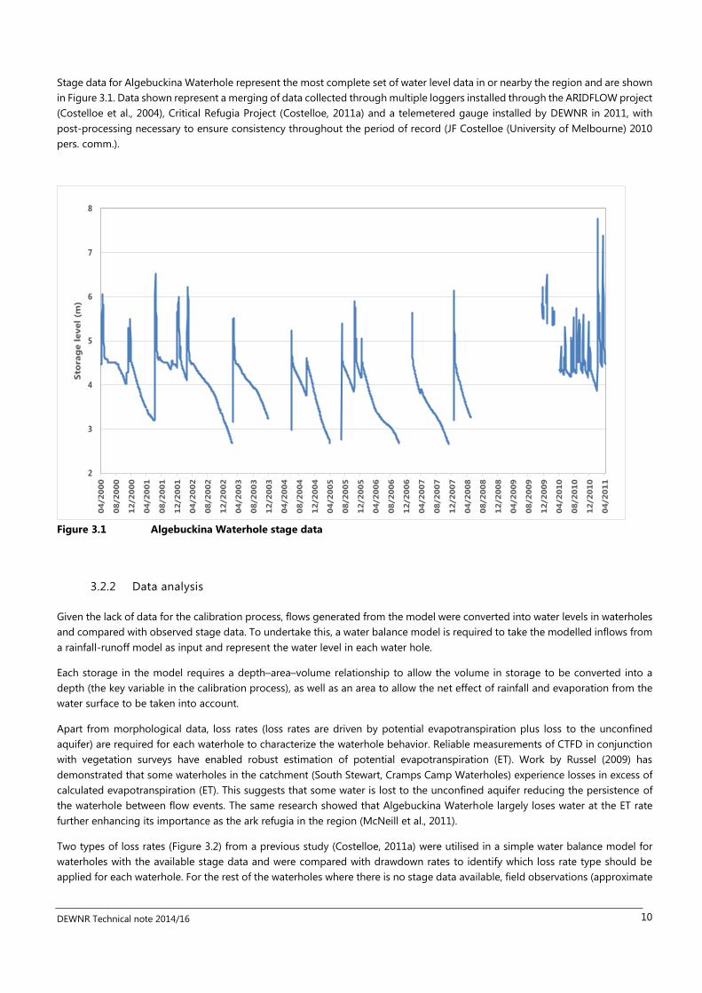
Two types of loss rates (Figure 3.2) from a previous study (Costelloe, 2011a) were utilised in a simple water balance model for

waterholes with the available stage data and were compared with drawdown rates to identify which loss rate type should be

applied for each waterhole. For the rest of the waterholes where there is no stage data available, field observations (approximate

2

3

4

5

6

7

8

04

/2

00

0

08

/2

00

0

12

/2

00

0

04

/2

00

1

08

/2

00

1

12

/2

00

1

04

/2

00

2

08

/2

00

2

12

/2

00

2

04

/2

00

3

08

/2

00

3

12

/2

00

3

04

/2

00

4

08

/2

00

4

12

/2

00

4

04

/2

00

5

08

/2

00

5

12

/2

00

5

04

/2

00

6

08

/2

00

6

12

/2

00

6

04

/2

00

7

08

/2

00

7

12

/2

00

7

04

/2

00

8

08

/2

00

8

12

/2

00

8

04

/2

00

9

08

/2

00

9

12

/2

00

9

04

/2

01

0

08

/2

01

0

12

/2

01

0

04

/2

01

1

Sto

rag

e l

evel

(m)


timing from filling to drying states) were used to adopt one of those two loss rates. From these comparisons the uncertainty of

the duration of drying period is likely to be less than two months.

Figure 3.2 Average monthly loss rate for Neales-Peake catchment waterholes

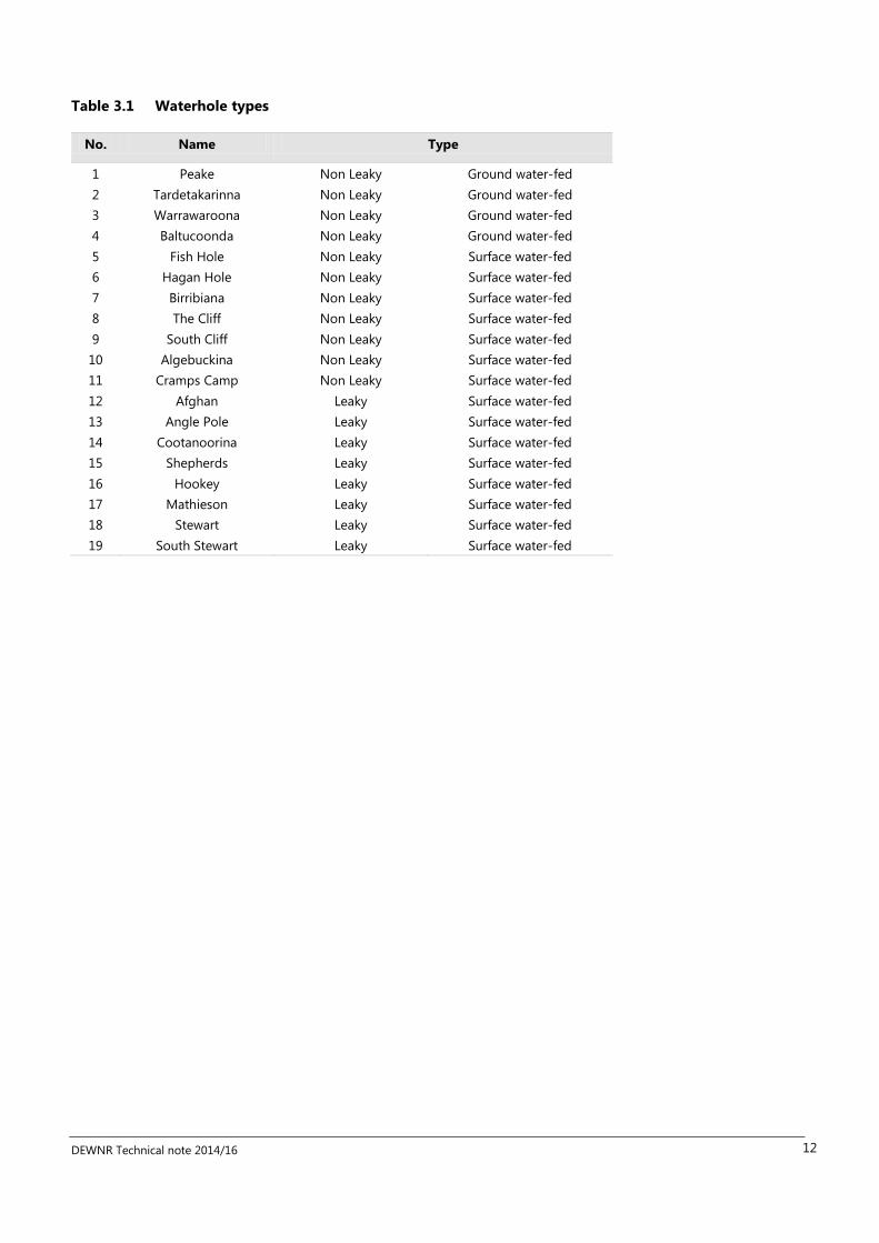
Waterholes are categorised based on their loss rates in Table 3.1. The variability in loss rates across the region suggests that the

waterholes located at the upper part of the catchment have higher loss rates than the waterholes in the downstream part which

is consistent with the fact that the groundwater table is deeper in the upper part of the catchment than in the lower part. Storage

dimensions and daily time series of total loss (Evaporation + Seepage) were imported into each storage node in the model using

the storage editor’s window, further details of which are presented in the next section.

0

0.05

0.1

0.15

0.2

0.25

0.3

0.35

0.4

JAN FEB MAR APR MAY JUN JUL AUG SEP OCT NOV DEC

Avera

ge M

on

thly

Lo

ss R

ate

, m

Non Leaky Waterhole Leaky Waterhole


Table 3.1 Waterhole types

No. Name Type

1 Peake Non Leaky Ground water-fed

2 Tardetakarinna Non Leaky Ground water-fed

3 Warrawaroona Non Leaky Ground water-fed

4 Baltucoonda Non Leaky Ground water-fed

5 Fish Hole Non Leaky Surface water-fed

6 Hagan Hole Non Leaky Surface water-fed

7 Birribiana Non Leaky Surface water-fed

8 The Cliff Non Leaky Surface water-fed

9 South Cliff Non Leaky Surface water-fed

10 Algebuckina Non Leaky Surface water-fed

11 Cramps Camp Non Leaky Surface water-fed

12 Afghan Leaky Surface water-fed

13 Angle Pole Leaky Surface water-fed

14 Cootanoorina Leaky Surface water-fed

15 Shepherds Leaky Surface water-fed

16 Hookey Leaky Surface water-fed

17 Mathieson Leaky Surface water-fed

18 Stewart Leaky Surface water-fed

19 South Stewart Leaky Surface water-fed


4 Surface water modelling

4.1 Overview

Reliable estimates of arid zone streamflow are required to inform and support policy and decision makers in water planning and

management. A variety of methods are available to determine or estimate routed streamflow through catchments. Observed

data are best wherever possible, but alternatively, estimates can be provided by using empirical and statistical techniques, and

more commonly using hydrological models (Vaze, et al., 2012, p. 5).

Hydrological modelling can be undertaken using a range of approaches, such as, simple empirical methods, large scale energy-

water balance equations, conceptual hydrological models, landscape hydrological models and fully distributed physically based

hydrological models. The choice of modelling approach is driven by various factors, with problem definition (purpose of the

modelling exercise) and data availability being two key factors. Conceptual hydrological modelling is the commonly used

category for investigations of this type. Description of other hydrological modelling categories and their applications are

provided in ‘Guidelines for rainfall-runoff modelling: Towards best practice model application’ (Vaze, et al., 2012).

Conceptual hydrological models are simplified conceptual representations of different components of the hydrological cycle and

the interactions between them (e.g. rainfall, evaporation, interception, storage, infiltration, surface runoff, groundwater recharge

and base flow). These components and their interactions are described mathematically by equations that form the basis of the

model.

4.2 Modelling objective

The objective of this modelling was to deliver a tool that will (i) aid in assessing the impacts on the flow regime if mining

operations were to within the Neales-Peake catchment and (ii) aid in ecohydrological assessment of the region. To address this

objective a hydrological model was built and calibrated to observed stage data in the region.

4.3 Methodology

The hydrological modelling platform used for this study was Source (Carr, R, Podger, G., 2012). Source is a nationally recognised

hydrological modelling platform that has been developed as part of an Australia-wide collaboration and which has been

endorsed by the Australian Government. Source is a PC-based rainfall-runoff and flow routing water balance modelling platform.

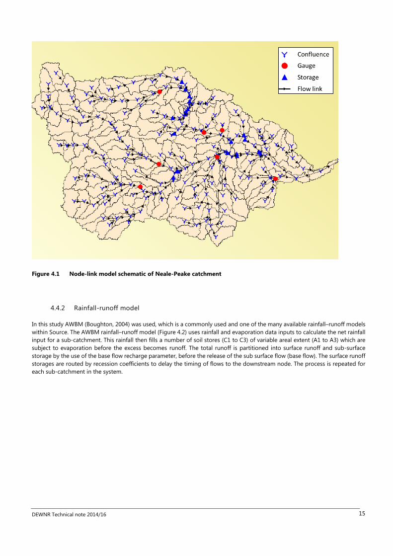
Within Source, a model is constructed as a series of nodes and links which are connected based on the drainage direction of the

catchment being modelled. Each node/link can represent different components of the water balance, such as:

confluences (the meeting of two or more streamlines)

splitters (locations where the channel branches into two or more drainage lines)

storages (lakes, waterholes, etc.)

inflow nodes (locations where flow is added to the system).

A hydrological model has been constructed and calibrated in Source for the Neales-Peake Catchment using delineated sub-

catchments, observed daily rainfall data, evaporation data, stage data, waterhole properties (e.g. volume and surface area), and

estimated catchment parameters.


4.4 Model construction

Model construction is the process of:

delineating the catchment into sub-catchments (described in Section 2.3)

creating and parameterising nodes and links to represent the hydrological components, behaviour and characteristics

of the catchment

defining the interactions between the various processes of the hydrological cycle included in the model.

4.4.1 Nodes

4.4.1.1 Confluences

Confluences or catchment nodes incorporate information about the inflows from the sub-catchment area they are assigned to,

such as:

sub-catchment area

rainfall and evaporation data for the station associated with the sub-catchment

model catchment parameters for the functional units within the sub-catchment

spatial location.

4.4.1.2 Storage nodes

Storage nodes are used to simulate the water balance model for each individual waterhole. Input data required for a waterhole

water balance model include:

depth-area-volume relationship

initial volume (assumed to be empty)

rainfall data for the waterhole location

loss rate from the waterhole (evaporation + leakage to groundwater)

spillway information.

Assumptions and information regarding waterholes are given in Section 3.2.

4.4.1.3 Controlled splitter nodes

Controlled splitter nodes are used to split the sub-catchment flow according to the ‘free-to-flow’ area (as a proportion of the

total sub-catchment area), allowing floods to flow to two parallel waterholes. These nodes distribute flow down a main and an

effluent branch according to a fixed percentage that can be a function of flow. There are two splitter nodes in the source model

for Neales-Peake catchment and it is assumed that flow is equally distributed between main and effluent branches since no

evidence suggested that one branch was preferred over another.

4.4.1.4 Gauge nodes

Streamflow gauges nodes represent the location of a site with streamflow records. This is only used in model validation, since

there is no cross sectional information at the location of the stage loggers to convert stage data to flow. However, data at these

points can be used to validate the timing of floods across the whole catchment.

Figure 4.1 is a schematic of the hydrological model built in Source for the Neales-Peake catchment.


Figure 4.1 Node-link model schematic of Neale-Peake catchment

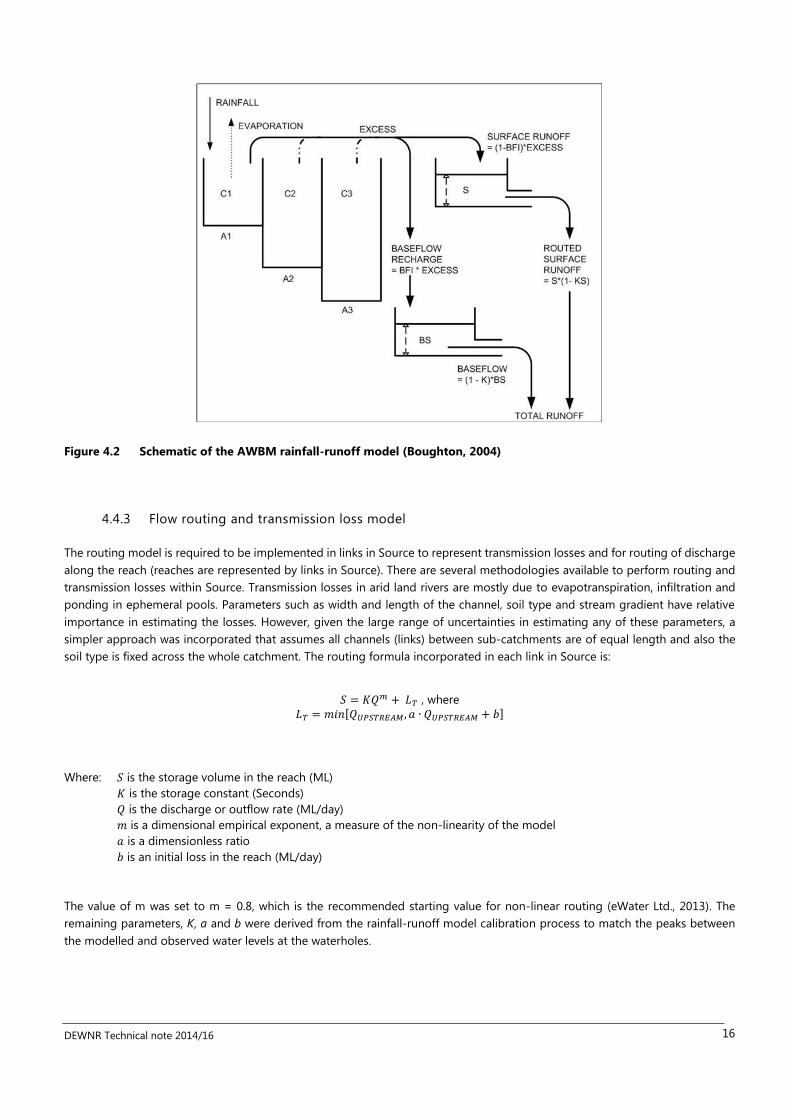
4.4.2 Rainfall-runoff model

In this study AWBM (Boughton, 2004) was used, which is a commonly used and one of the many available rainfall–runoff models

within Source. The AWBM rainfall–runoff model (Figure 4.2) uses rainfall and evaporation data inputs to calculate the net rainfall

input for a sub-catchment. This rainfall then fills a number of soil stores (C1 to C3) of variable areal extent (A1 to A3) which are

subject to evaporation before the excess becomes runoff. The total runoff is partitioned into surface runoff and sub-surface

storage by the use of the base flow recharge parameter, before the release of the sub surface flow (base flow). The surface runoff

storages are routed by recession coefficients to delay the timing of flows to the downstream node. The process is repeated for

each sub-catchment in the system.


Figure 4.2 Schematic of the AWBM rainfall-runoff model (Boughton, 2004)

4.4.3 Flow routing and transmission loss model

The routing model is required to be implemented in links in Source to represent transmission losses and for routing of discharge

along the reach (reaches are represented by links in Source). There are several methodologies available to perform routing and

transmission losses within Source. Transmission losses in arid land rivers are mostly due to evapotranspiration, infiltration and

ponding in ephemeral pools. Parameters such as width and length of the channel, soil type and stream gradient have relative

importance in estimating the losses. However, given the large range of uncertainties in estimating any of these parameters, a

simpler approach was incorporated that assumes all channels (links) between sub-catchments are of equal length and also the

soil type is fixed across the whole catchment. The routing formula incorporated in each link in Source is:

𝑆 = 𝐾𝑄𝑚 + 𝐿𝑇 , where

𝐿𝑇 = 𝑚𝑖𝑛[𝑄𝑈𝑃𝑆𝑇𝑅𝐸𝐴𝑀 , 𝑎 ∙ 𝑄𝑈𝑃𝑆𝑇𝑅𝐸𝐴𝑀 + 𝑏]

Where: 𝑆 is the storage volume in the reach (ML)

𝐾 is the storage constant (Seconds)

𝑄 is the discharge or outflow rate (ML/day)

𝑚 is a dimensional empirical exponent, a measure of the non-linearity of the model

𝑎 is a dimensionless ratio

𝑏 is an initial loss in the reach (ML/day)

The value of m was set to m = 0.8, which is the recommended starting value for non-linear routing (eWater Ltd., 2013). The

remaining parameters, K, a and b were derived from the rainfall-runoff model calibration process to match the peaks between

the modelled and observed water levels at the waterholes.


4.5 Model calibration and validation

Model calibration is a process of optimising model parameter values to get a set of parameters which provides the best estimate

of the observed streamflow (Vaze, 2012). By comparing modelled data against observed records, the degree of correlation

between the two datasets can be assessed. The iterative process of varying catchment input parameters is undertaken until a

‘good correlation’ is achieved between the simulated and observed datasets. The purpose of calibration is to ensure the model

is able to adequately represent the hydrological behaviour of the catchment.

Model validation is usually a process of using the calibrated model parameters to simulate runoff over an independent period

outside the calibration period (Vaze, 2012). This is undertaken to evaluate the suitability of the calibrated model for predicting

runoff over a period outside the calibration period. Validation is considered an important step in the modelling process as it

increases the confidence in the ability of the model to undertake prediction. However, in this study different characteristics of

the catchment were studied as validation process. For example, there are some waterholes with no stage data available to be

used for calibration, but there are some field observations that indicate when those waterholes dried. These observations were

then used to validate the calibrated parameters.

AWBM, which is one of the catchment rainfall-runoff models in the Source platform, was used in this study. A description of the

model is provided in Section 4.4.2. The input parameters that were varied during calibration were the parameters of the AWBM

rainfall-runoff model and the input parameters of the routing and transmission loss model across the catchment. These

parameters are listed in Appendix B.

For the purposes of this study, ‘good correlation’ involved visual and statistical comparison of observed and simulated storage

level data at daily timescale. This is further discussed in Section 4.5.2.

4.5.1 Calibration method

The inbuilt Source ‘Calibration Wizard’ was considered not appropriate for use in this study, as it requires adequate flow data to

perform a calibration analysis. As discussed in Section 3.2.1, since adequate flow data are not available for this region, water level

records were instead used for calibration. The water level records for the following waterholes were used for calibration:

Algebuckina

Afghan

South Stewart

Peake

Manual calibration was performed to produce one optimum set of inputs (Appendix B) and assist the process of predicting flow

data that accord with daily stage data. To undertake this, input parameter sets for the AWBM rainfall-runoff model were

populated with pre-calibrated model parameters provided through Ryu et al., 2014 with the model then run iteratively and

selected statistical measures checked to achieve the best calibration possible. Visual comparison of the two datasets at daily

timescales was also used.

4.5.2 Calibration results

The following statistical measures were used to verify the effectiveness of calibration:

Percentage difference from mean

Coefficient of determination (R2)

Nash-Sutcliffe coefficient of efficiency (NSE).

Using the statistical measures listed above, observed and modelled storage levels in waterholes were compared at a daily

timescale. The two datasets at a daily timescale for each studied waterhole are shown in Figure 4.3 to Figure 4.6.

A summary of daily calibration statistics is provided in Table 4.1.


Table 4.1 Daily calibration statistics

R2 describes the proportion of the variance in these data that can be explained by the model. R2 can range between 0 and 1.0,

with higher values (i.e. closer to one) describing a better fit.

NSE defined by Nash and Sutcliffe (1970) is the ratio of the mean square error to the variance subtracted from one. It can range

between -∞ (negative infinity) and 1.0. A value of one describes a perfect fit, a value of zero indicates that the mean value for

the time step is an equally good predictor than the model, and a value of less than one indicates that the mean would be a better

predictor than the model.

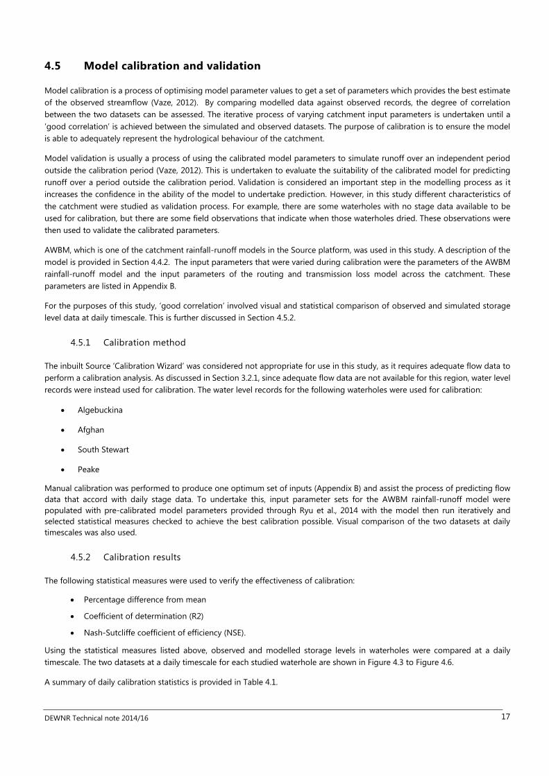
The R2 and NSE values (Table 4.1) for the each of the waterholes used for calibration indicate a good correlation between

observed and modelled data. Investigation of the daily hydrographs indicate, that in general, the model is able to simulate most

of the flow events and their duration quite close to the observed events. However, the difficulty appears to be in the simulation

of the magnitude of those events as shown in Figure 4.3 to Figure 4.6.

Figure 4.3 Observed and modelled water levels for Afghan Waterhole

0

1

2

3

4

5

08

/20

10

09

/20

10

11

/20

10

01

/20

11

02

/20

11

04

/20

11

06

/20

11

07

/20

11

09

/20

11

10

/20

11

12

/20

11

02

/20

12

03

/20

12

05

/20

12

07

/20

12

Sto

rag

e l

evel (m

)

Observed Modelled

Measures Afghan WH Sth Stewart WH Algebuckina WH Peake WH

Observed Modelled Observed Modelled Observed Modelled Observed Modelled

Mean (m) 1.12 1.23 2.31 1.95 4.04 4.09 1.74 1.61

Median (m) 1.06 1.17 2.35 2.1 4.13 4.32 1.69 1.72

R2 0.64 0.57 0.65 0.31

NSE 0.21 0.09 0.19 -1.29

% Difference from mean

9.48% 18.41% 1.23% -7.27%


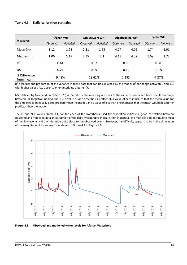
Figure 4.4 Observed and modelled water levels for South Stewart Waterhole

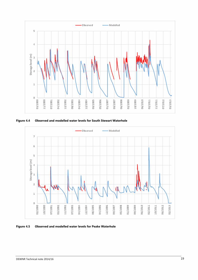
Figure 4.5 Observed and modelled water levels for Peake Waterhole


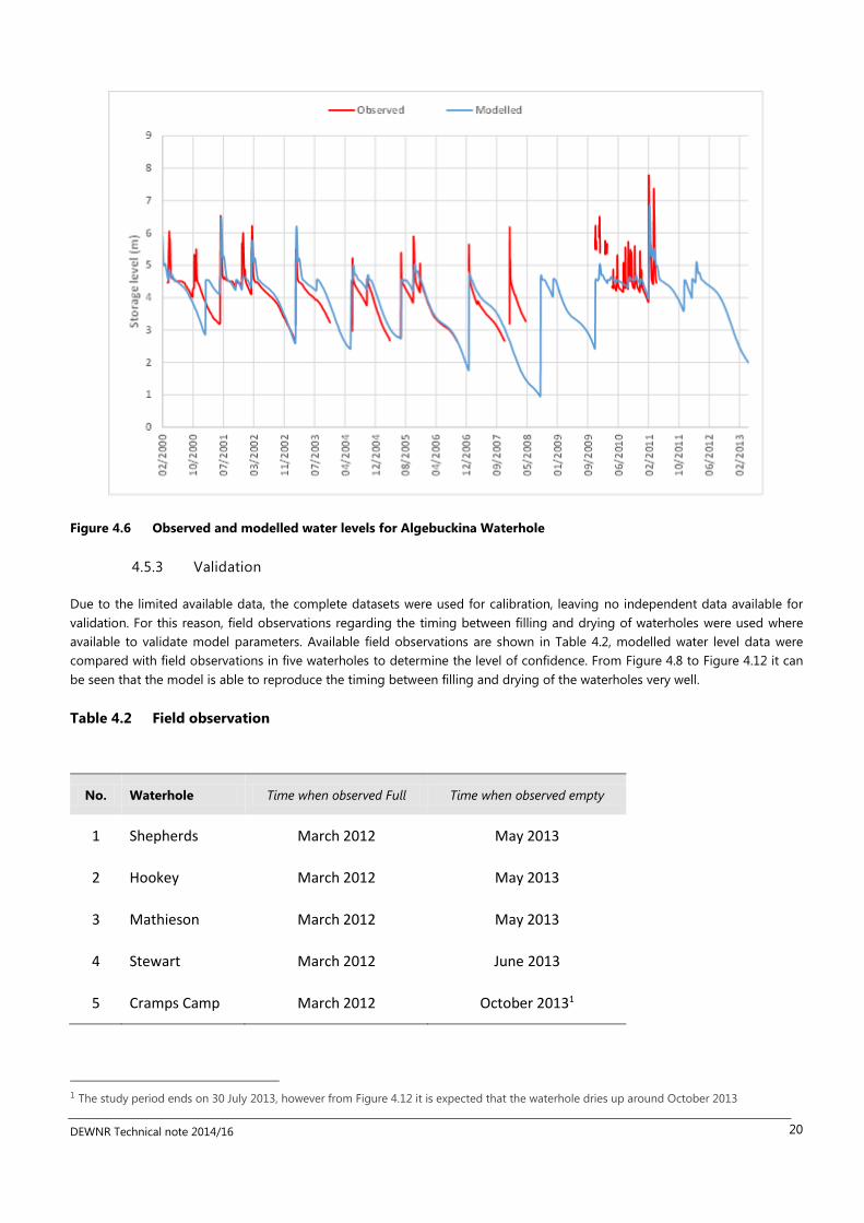
Figure 4.6 Observed and modelled water levels for Algebuckina Waterhole

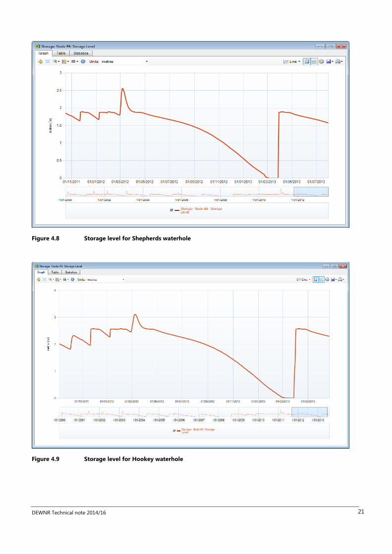
4.5.3 Validation

Due to the limited available data, the complete datasets were used for calibration, leaving no independent data available for

validation. For this reason, field observations regarding the timing between filling and drying of waterholes were used where

available to validate model parameters. Available field observations are shown in Table 4.2, modelled water level data were

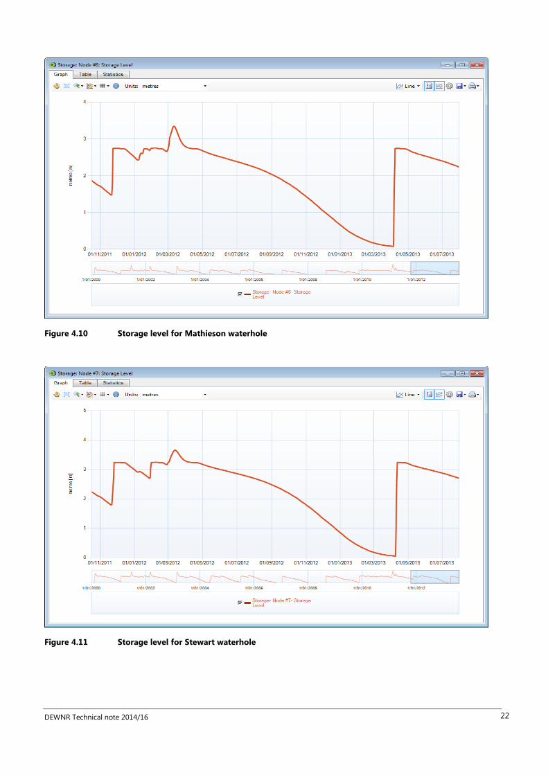
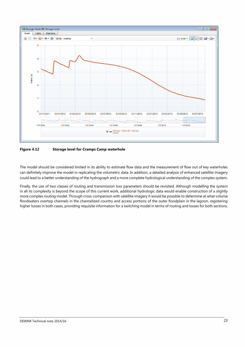
compared with field observations in five waterholes to determine the level of confidence. From Figure 4.8 to Figure 4.12 it can

be seen that the model is able to reproduce the timing between filling and drying of the waterholes very well.

Table 4.2 Field observation

1 The study period ends on 30 July 2013, however from Figure 4.12 it is expected that the waterhole dries up around October 2013

No. Waterhole Time when observed Full Time when observed empty

1 Shepherds March 2012 May 2013

2 Hookey March 2012 May 2013

3 Mathieson March 2012 May 2013

4 Stewart March 2012 June 2013

5 Cramps Camp March 2012 October 20131


Figure 4.8 Storage level for Shepherds waterhole

Figure 4.9 Storage level for Hookey waterhole


Figure 4.10 Storage level for Mathieson waterhole

Figure 4.11 Storage level for Stewart waterhole


Figure 4.12 Storage level for Cramps Camp waterhole

The model should be considered limited in its ability to estimate flow data and the measurement of flow out of key waterholes

can definitely improve the model in replicating the volumetric data. In addition, a detailed analysis of enhanced satellite imagery

could lead to a better understanding of the hydrograph and a more complete hydrological understanding of the complex system.

Finally, the use of two classes of routing and transmission loss parameters should be revisited. Although modelling the system

in all its complexity is beyond the scope of this current work, additional hydrologic data would enable construction of a slightly

more complex routing model. Through cross-comparison with satellite imagery it would be possible to determine at what volume

floodwaters overtop channels in the channelized country and access portions of the outer floodplain in the lagoon, registering

higher losses in both cases, providing requisite information for a switching model in terms of routing and losses for both sections.


5 Summary and recommendations for future

work

This report details the construction of a rainfall-runoff and flow routing model for the Neales-Peake catchment in the Source

modelling platform. The model uses the Australian Water Balance rainfall/runoff Model (AWBM) to generate runoff for 177 sub-

catchments and routes this flow through the system to discharge at Lake Eyre North, accounting for 20 waterhole storages.

Detailed bathymetry of the waterholes in the system, in addition to observations regarding surface-water/groundwater

interactions at the waterholes, was incorporated into the model, ensuring that waterhole dynamics were accurately represented

by the model.

The model was calibrated by comparing modelled stage heights with those heights observed at four key waterholes. The limited

and patchy nature of the data coverage over the study region means that traditional calibration statistics may be misleading.

This being said, the model was able to reproduce observed stage, with an average difference of 6.5% between modelled and

observed median stage height across the waterholes. This translated to an average difference of approximately 9% in average

storage volume. Additionally, it was shown visually that the model tended to replicate the timing of events very well. At each

waterhole the model struggled to identify some smaller flow events, in particular multiple flow events, however it did not register

any false positives and as such was considered fit for purpose.

To assist in validating the model, the wetting and drying cycles at waterholes were compared with field observations. The model

was also able to reproduce these observations, within one month of what was observed. Given the vagaries surrounding the

timing of field observations, this can be regarded as a reasonable result which indicates that the flow routing models are

consistent with observations.

Although the model is able to reproduce the timing of observed events in the system very well, the model should be considered

limited in its ability to estimate the magnitude of the events. The lack of volumetric information to calibrate the model means

that it is not possible to estimate confidence surrounding simulated discharge volumes.

Recommendations for future work fall into two complementary categories, data collection and model refinement. By conducting

flow gaugings at strategic locations throughout the system a measure of confidence in simulated flow volumes could be gained.

Additionally, more detailed information regarding the surface-water/groundwater interactions at waterholes and throughout the

system would enable a more complete representation of the hydrological dynamics of the catchment. Data that have been

collected are often inconsistent owing to malfunctioning loggers, disturbance from local fauna, theft and varying installation and

removal dates. Establishment of a more permanent monitoring network and the collection of data that come from such a network

would enable continuous refinement of model parameters and deliver a better understanding of the hydrology of the system.

The Neales-Peake Catchment has a varied geography, containing a diverse range of country – from the red sands of the Pedirka

Desert to the hard packed clays of the gibber pans. Furthermore, the watercourses of the Neales-Peake are equally varied, ranging

from well-defined incised channels to poorly channelized floodplains. As such, it is unlikely that the rainfall-runoff response and

transmission losses will be consistent throughout the catchment as considered in the model. More comprehensive data on land

type, supplemented by hydrological observations, would allow the calibration of discrete rainfall-runoff and transmission loss

models within sub-regions of the catchment that share similar geography and hydrology.


6 References

1 Boughton, W. C. (2004) The Australian water balance model, Environmental Modelling and Software, 19,943-956.

2 Costelloe J. F., Hudson P. J., Pritchard J. C., Puckridge J. T. and Reid J. R. W. (2004) ARIDFLO Scientific Report:

Environmental Flow Requirements of Arid Zone Rivers with Particular Reference to the Lake Eyre Drainage

Basin.Final Report to South Australian Department of Water, Land and Biodiversity Conservation and

Commonwealth Department of Environment and Heritage. School of Earth and Environmental Sciences, University

of Adelaide, Adelaide.

3 Carr, R., Podger, G., 2012. eWater Source - Australia's next generation IWRM modelling platform, 34th Hydrology

and Water Resources Symposium December 2012.

4 Costelloe J. F., Grayson R. B. and McMahon T. A. (2005a) Modelling streamflow in a large ungauged arid zone river,

central Australia, for use in ecological studies. Hydrological Processes 19: 1165-1183.

5 Costelloe J. F., Shields A., Grayson R. B., and McMahon T. A. (2007a) Determining loss characteristics of arid zone

river waterbodies. River Res. Appl. 23: 715-731, doi: 10.1002/rra.991

6 Costelloe J. F. (2011a) Hydrological assessment and analysis of the Neales Catchment, Report to the South

Australian Arid Lands Natural Resources Management Board, Port Augusta.

7 eWater Ltd (2013). Source User Guide (v3.5.0).

[https://ewater.atlassian.net/wiki/display/SD35/Source+User+Guide]

8 Jeffrey, S.J., Carter, J.O., Moodie, K.B. and Beswick, A.R. (2001). Using spatial interpolation to construct a comprehensive

archive of Australian climate data External link icon, Environmental Modelling and Software, Vol 16/4, pp 309-330.

8 McNeil D., Schmarr D. and Rosenberger A. (2011) Climatic variability, fish and the role of refuge waterholes in the

Neales River catchment: Lake Eyre Basin, South Australia, Report to the South Australian Arid Lands Natural

Resources Management Board.

9 Russell K. (2009) Determining loss characteristics of arid zone river waterbodies – final report. 4th year

undergraduate research report, University of Melbourne.

10 Ryu, D., J. Costelloe, R. Pipunic, and C.-H. Su, (2014) Rainfall-runoff modelling of the Neales River catchment. Report

to the South Australian Department of Environment, Water and Natural Resources.

11 The State of Queensland, (2013) SILO Climate Data, Department of Science, Information Technology, Innovation

and the Arts, viewed 27 May 2013, <http://www.longpaddock.qld.gov.au/silo/about.html>

12 Vaze, J., Jordan, P., Beecham, R., Frost, A., Summerell, G. (2012) Guidelines for rainfall -runoff modelling: Towards

best practise model application’. eWater Ltd.

13 Wakelin-King, G.A., (2011) Geomorphological assessment and analysis of the Neales Catchment: A report to the

South Australian Arid Lands Natural Resources Management Board. Wakelin Associates, Melbourne.

http://www.longpaddock.qld.gov.au/silo/about.html


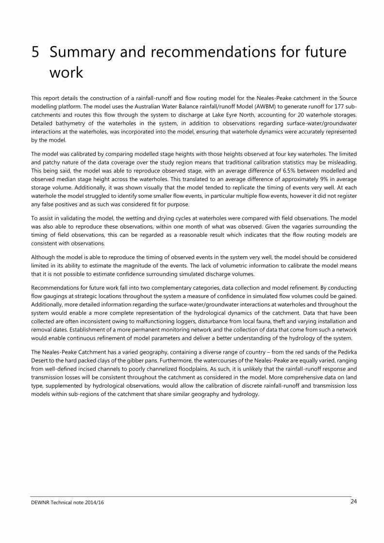
Appendix A: Waterholes bathymetry

relationships

Figure 1 Bathymetry relationship for Afghan Waterhole

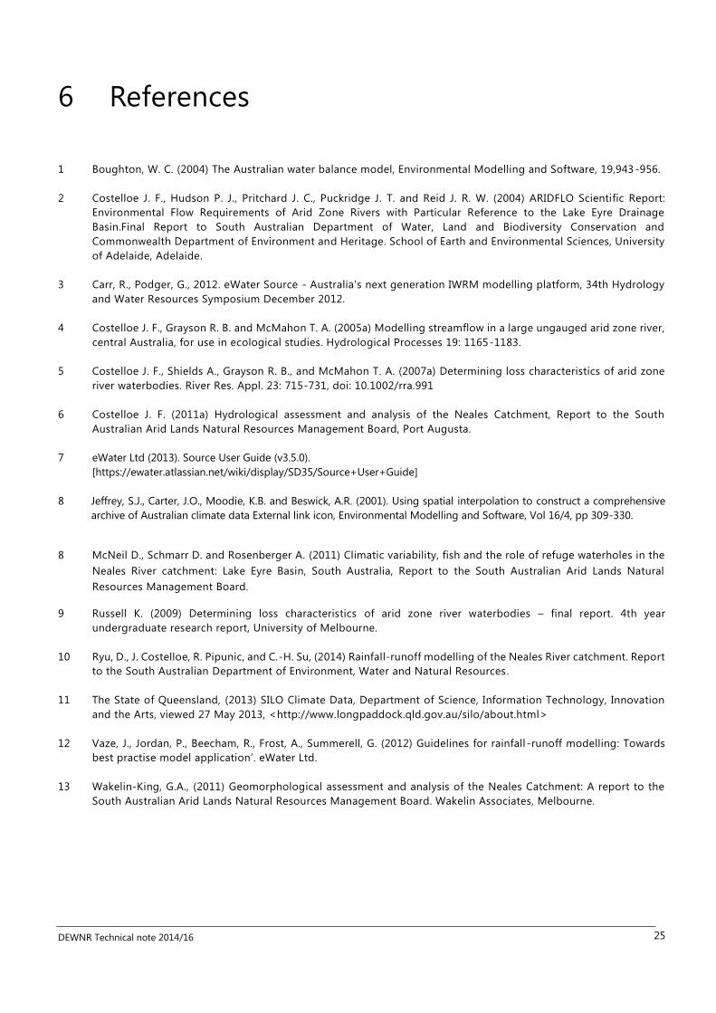
Figure 2 Bathymetry relationship for Angle Pole Waterhole

0

0.1

0.2

0.3

0.4

0.5

0.6

0.7

0.8

0.9

0

1

2

3

4

5

6

7

0 0.2 0.4 0.6 0.8 1 1.2 1.4

Are

a, H

a

Vo

lum

e, M

L

Elevation, m

Volume, ML Area, Ha

0.00

0.20

0.40

0.60

0.80

1.00

1.20

1.40

1.60

0.0

2.0

4.0

6.0

8.0

10.0

12.0

14.0

16.0

0 0.5 1 1.5 2 2.5

Are

a, H

a

Vo

lum

e, M

L

Elevation, m

Volume, ML Area, Ha


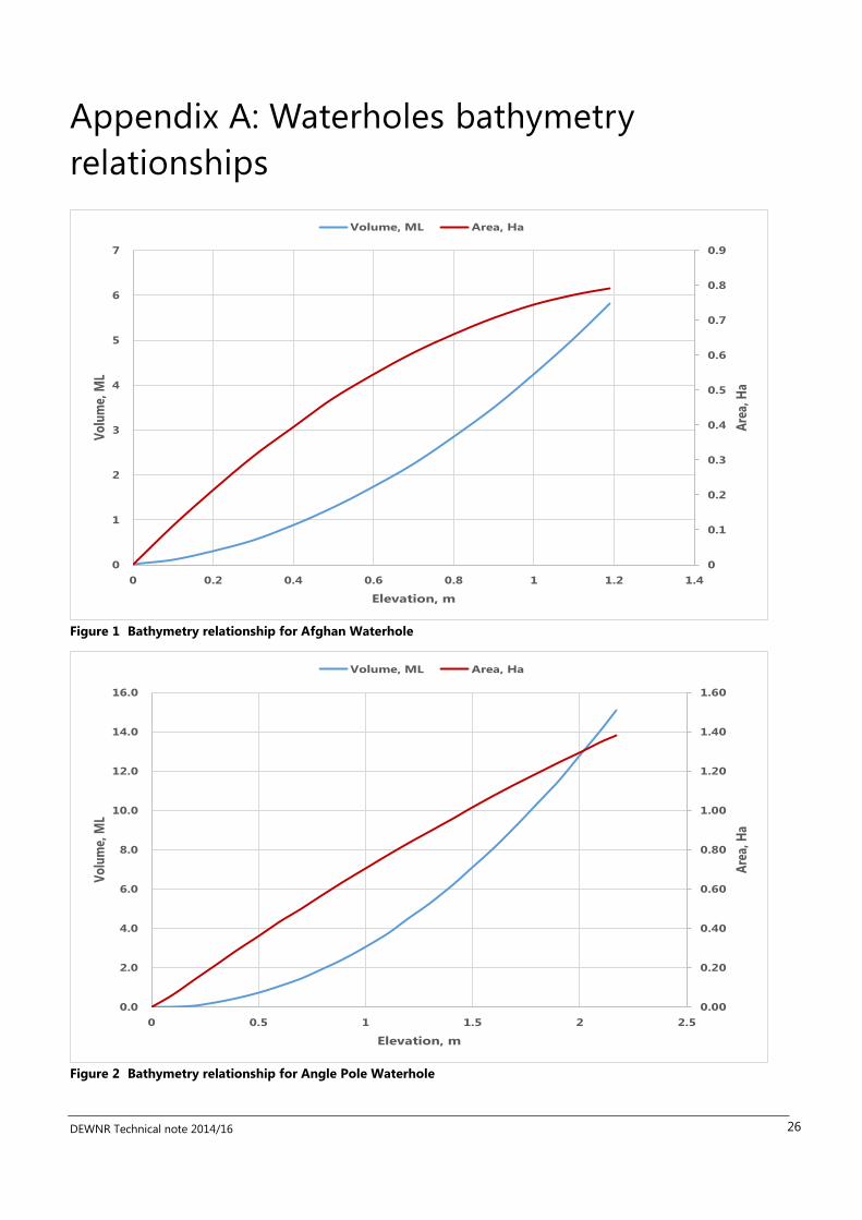
Figure 3 Bathymetry relationship for Shepherds Waterhole

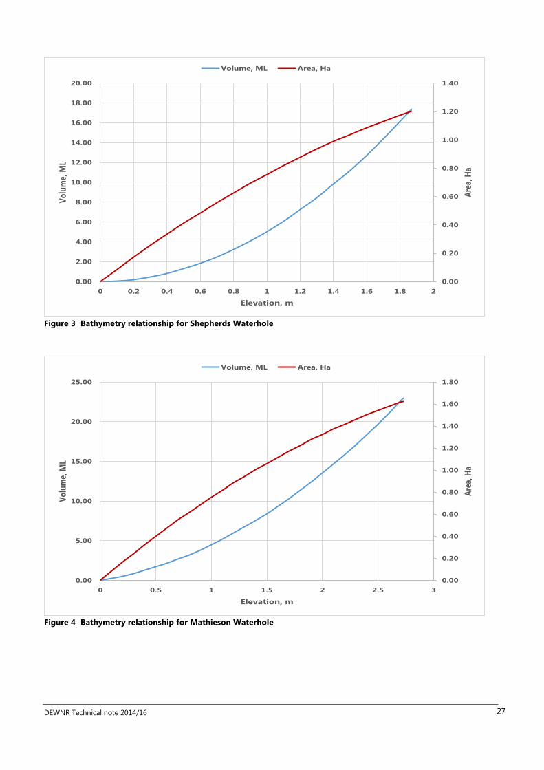
Figure 4 Bathymetry relationship for Mathieson Waterhole

0.00

0.20

0.40

0.60

0.80

1.00

1.20

1.40

0.00

2.00

4.00

6.00

8.00

10.00

12.00

14.00

16.00

18.00

20.00

0 0.2 0.4 0.6 0.8 1 1.2 1.4 1.6 1.8 2

Are

a, H

a

Vo

lum

e, M

L

Elevation, m

Volume, ML Area, Ha

0.00

0.20

0.40

0.60

0.80

1.00

1.20

1.40

1.60

1.80

0.00

5.00

10.00

15.00

20.00

25.00

0 0.5 1 1.5 2 2.5 3

Are

a, H

a

Vo

lum

e, M

L

Elevation, m

Volume, ML Area, Ha


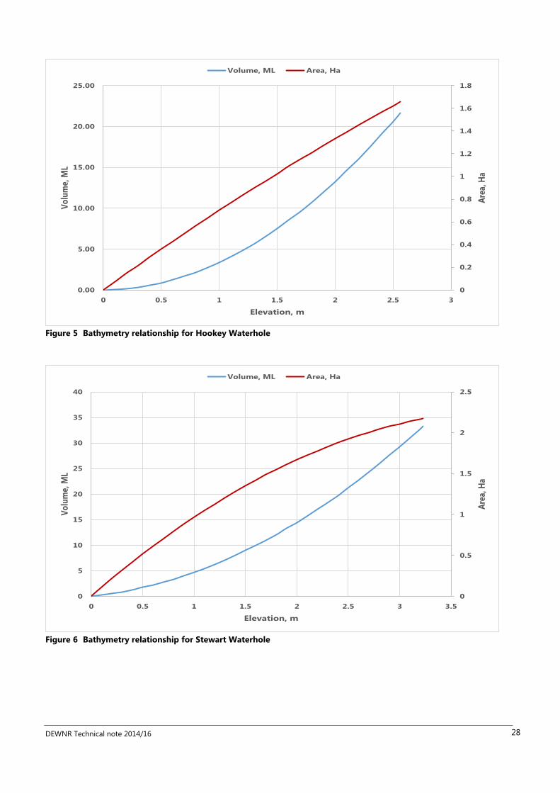
Figure 5 Bathymetry relationship for Hookey Waterhole

Figure 6 Bathymetry relationship for Stewart Waterhole

0

0.2

0.4

0.6

0.8

1

1.2

1.4

1.6

1.8

0.00

5.00

10.00

15.00

20.00

25.00

0 0.5 1 1.5 2 2.5 3

Are

a, H

a

Vo

lum

e, M

L

Elevation, m

Volume, ML Area, Ha

0

0.5

1

1.5

2

2.5

0

5

10

15

20

25

30

35

40

0 0.5 1 1.5 2 2.5 3 3.5

Are

a, H

a

Vo

lum

e, M

L

Elevation, m

Volume, ML Area, Ha


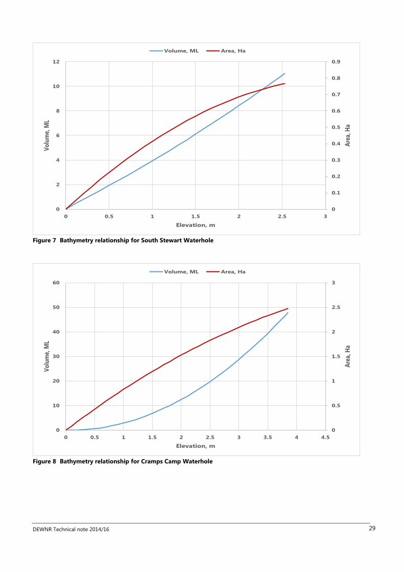
Figure 7 Bathymetry relationship for South Stewart Waterhole

Figure 8 Bathymetry relationship for Cramps Camp Waterhole

0

0.1

0.2

0.3

0.4

0.5

0.6

0.7

0.8

0.9

0

2

4

6

8

10

12

0 0.5 1 1.5 2 2.5 3

Are

a, H

a

Vo

lum

e, M

L

Elevation, m

Volume, ML Area, Ha

0

0.5

1

1.5

2

2.5

3

0

10

20

30

40

50

60

0 0.5 1 1.5 2 2.5 3 3.5 4 4.5

Are

a, H

a

Vo

lum

e, M

L

Elevation, m

Volume, ML Area, Ha


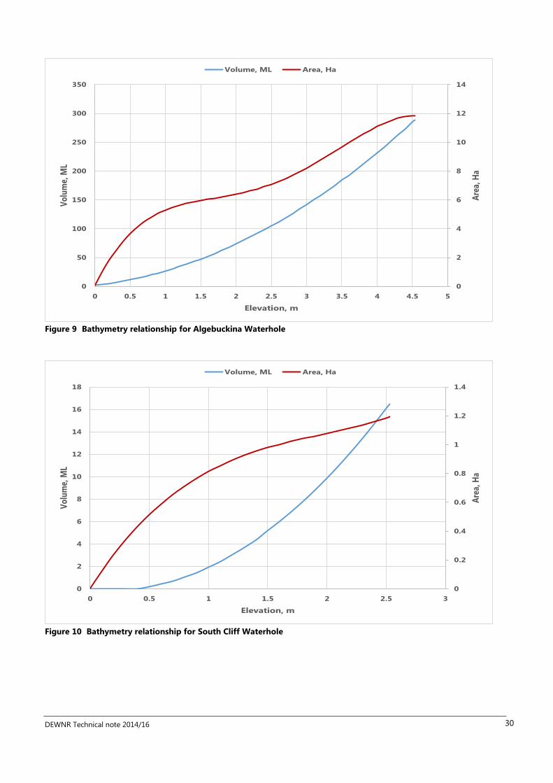
Figure 9 Bathymetry relationship for Algebuckina Waterhole

Figure 10 Bathymetry relationship for South Cliff Waterhole

0

2

4

6

8

10

12

14

0

50

100

150

200

250

300

350

0 0.5 1 1.5 2 2.5 3 3.5 4 4.5 5

Are

a, H

a

Vo

lum

e, M

L

Elevation, m

Volume, ML Area, Ha

0

0.2

0.4

0.6

0.8

1

1.2

1.4

0

2

4

6

8

10

12

14

16

18

0 0.5 1 1.5 2 2.5 3

Are

a, H

a

Vo

lum

e, M

L

Elevation, m

Volume, ML Area, Ha


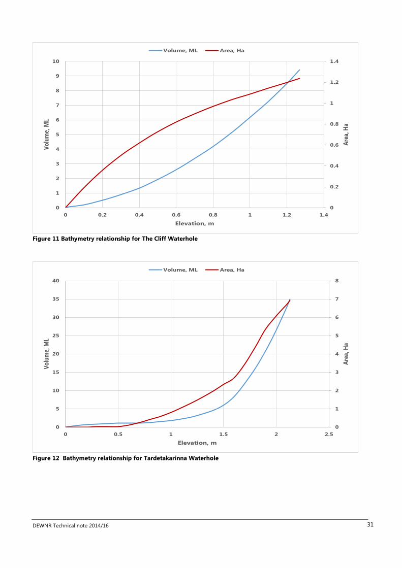
Figure 11 Bathymetry relationship for The Cliff Waterhole

Figure 12 Bathymetry relationship for Tardetakarinna Waterhole

0

0.2

0.4

0.6

0.8

1

1.2

1.4

0

1

2

3

4

5

6

7

8

9

10

0 0.2 0.4 0.6 0.8 1 1.2 1.4

Are

a, H

a

Vo

lum

e, M

L

Elevation, m

Volume, ML Area, Ha

0

1

2

3

4

5

6

7

8

0

5

10

15

20

25

30

35

40

0 0.5 1 1.5 2 2.5

Are

a, H

a

Vo

lum

e, M

L

Elevation, m

Volume, ML Area, Ha


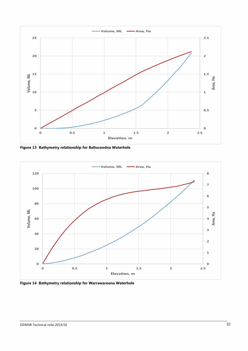
Figure 13 Bathymetry relationship for Baltucoodna Waterhole

Figure 14 Bathymetry relationship for Warrawaroona Waterhole

0

0.5

1

1.5

2

2.5

0

5

10

15

20

25

0 0.5 1 1.5 2 2.5

Are

a, H

a

Vo

lum

e, M

L

Elevation, m

Volume, ML Area, Ha

0

1

2

3

4

5

6

7

8

0

20

40

60

80

100

120

0 0.5 1 1.5 2 2.5

Are

a, H

a

Vo

lum

e, M

L

Elevation, m

Volume, ML Area, Ha


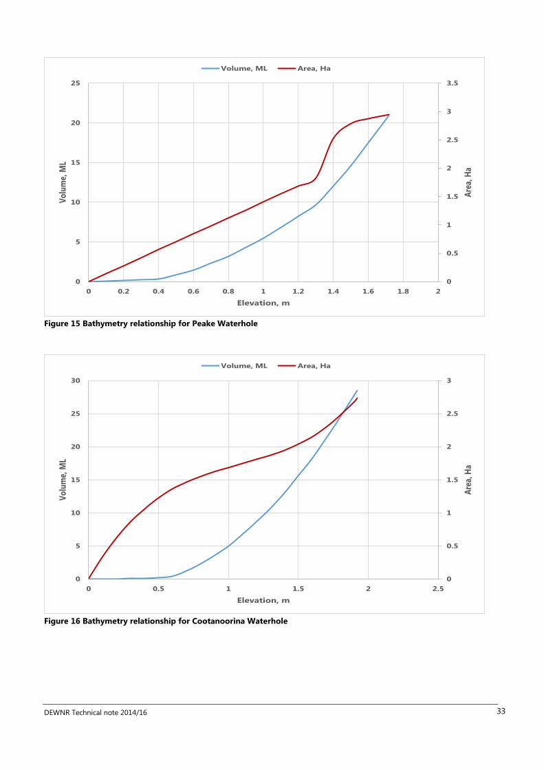
Figure 15 Bathymetry relationship for Peake Waterhole

Figure 16 Bathymetry relationship for Cootanoorina Waterhole

0

0.5

1

1.5

2

2.5

3

3.5

0

5

10

15

20

25

0 0.2 0.4 0.6 0.8 1 1.2 1.4 1.6 1.8 2

Are

a, H

a

Vo

lum

e, M

L

Elevation, m

Volume, ML Area, Ha

0

0.5

1

1.5

2

2.5

3

0

5

10

15

20

25

30

0 0.5 1 1.5 2 2.5

Are

a, H

a

Vo

lum

e, M

L

Elevation, m

Volume, ML Area, Ha


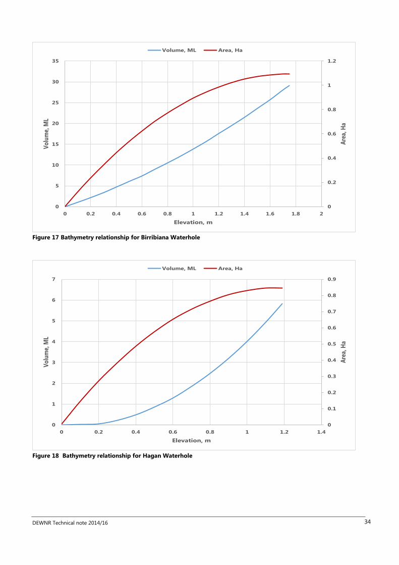
Figure 17 Bathymetry relationship for Birribiana Waterhole

Figure 18 Bathymetry relationship for Hagan Waterhole

0

0.2

0.4

0.6

0.8

1

1.2

0

5

10

15

20

25

30

35

0 0.2 0.4 0.6 0.8 1 1.2 1.4 1.6 1.8 2

Are

a, H

a

Vo

lum

e, M

L

Elevation, m

Volume, ML Area, Ha

0

0.1

0.2

0.3

0.4

0.5

0.6

0.7

0.8

0.9

0

1

2

3

4

5

6

7

0 0.2 0.4 0.6 0.8 1 1.2 1.4

Are

a, H

a

Vo

lum

e, M

L

Elevation, m

Volume, ML Area, Ha


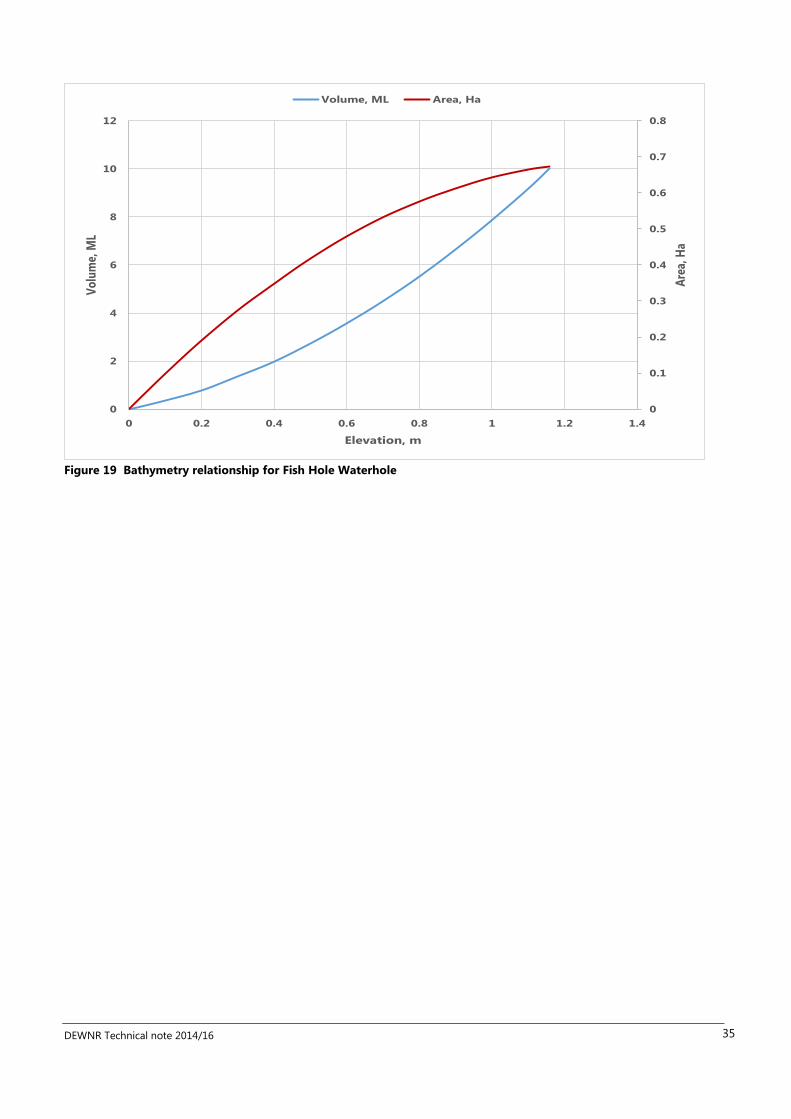
Figure 19 Bathymetry relationship for Fish Hole Waterhole

0

0.1

0.2

0.3

0.4

0.5

0.6

0.7

0.8

0

2

4

6

8

10

12

0 0.2 0.4 0.6 0.8 1 1.2 1.4

Are

a, H

a

Vo

lum

e, M

L

Elevation, m

Volume, ML Area, Ha


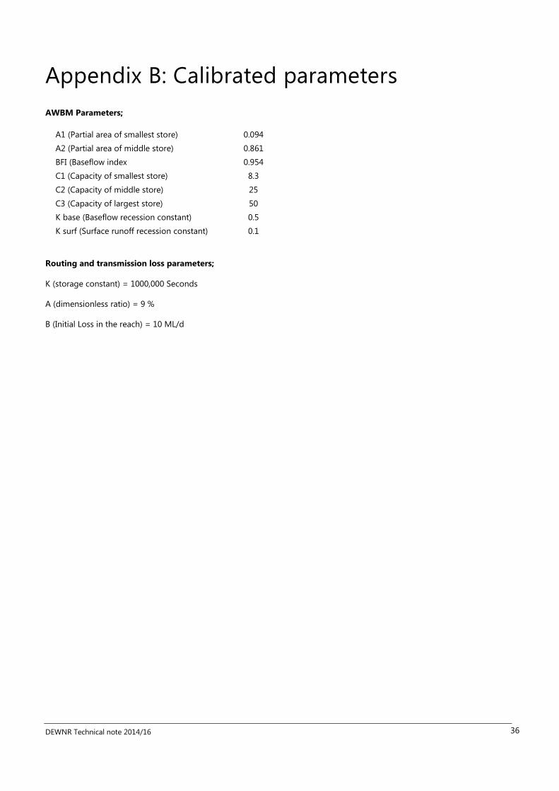
Appendix B: Calibrated parameters

AWBM Parameters;

A1 (Partial area of smallest store) 0.094

A2 (Partial area of middle store) 0.861

BFI (Baseflow index 0.954

C1 (Capacity of smallest store) 8.3

C2 (Capacity of middle store) 25

C3 (Capacity of largest store) 50

K base (Baseflow recession constant) 0.5

K surf (Surface runoff recession constant) 0.1

Routing and transmission loss parameters;

K (storage constant) = 1000,000 Seconds

A (dimensionless ratio) = 9 %

B (Initial Loss in the reach) = 10 ML/d

Hydrological assessment and analysis of Neales-Peake Catchment · Hydrological assessment and...

Documents

Transcript of Hydrological assessment and analysis of Neales-Peake Catchment · Hydrological assessment and...