UNIVERSITY OF NAIROBIcivil.uonbi.ac.ke/sites/default/files/cae/engineering/civil/Muna... ·...

UNIVERSITY OF NAIROBI

Hydrological Analysis of Sagana River (4A) Catchment

By Muna Benedict Waithaka, F16/2346/2009

A project submitted as a partial fulfillment

for the award of the degree of

BACHELOR OF SCIENCE IN CIVIL ENGINEERING

2014

You created this PDF from an application that is not licensed to print to novaPDF printer (http://www.novapdf.com)

http://www.novapdf.com

ABSTRACT

Sagana (4A) catchment is one of the most vital water tower basins in the country. Being part of

the vast Upper Tana River basin it has the seven forks dams, the Mwea Tabere irrigation scheme

among other significant installations. The catchment is a high rainfall zone, with rainfall depths

of approximately 2000mm per year. This is mainly due to the influence of the Aberdares and

Mt.Kenya as is evident from available rainfall data.

Using the maps available, the area of the catchment was found to be about 1600km2. These

maps, coupled with rainfall data from met dept was used to find the mean annual rainfall of the

Sagana catchment by methods like Isohyetal method and Thiessen polygon method. They both

gave close averages at 87.84mm and 86.75mm respectively. This is a big deviation from the

known average of about 150mm of rainfall.

The rainfall statistics are somewhat reflected in the streamflow data, in the seasonal variation of

river flow annually. Several analytics are done on the data to establish the catchments flow

characteristics. Flow duration curves (FDC), flow hydrographs, mass curves and low flow curves

are done to establish the margins of error and means for various aspects of river flow which

inform measures that can be taken to enhance reservoir management.

Sedimentation is a big concern for the catchment as increasing dead storage for the reservoirs

downstream is detrimental to their future. With some stations e.g. RGS 4AC05 and 4AC03

recording as much as 198tons/day and 156tons/day respectively, there is real cause for alarm.

Mitigation measures include better farming practices and tougher government regulations on

river and river bank usage.

Overall it’s established that the catchment has two rainfall seasons separated by a dry season.

Rainfall depth at stations near the two water towers is significantly higher. Stream flow

characteristics seem to be in tandem with rainfall characteristics too.



DEDICATION

This project is dedicated to Mum and Dad for their consistent encouragement, moral and financial support throughout the span of this study. Without them, this whole effort would lack the glow and brilliance that so characterizes it.

Also to a great extent, I would like to dedicate this project to God Almighty for his guidance, comfort, strength and breakthroughs that I witnessed through the entire process. Glory be to God.



Acknowledgements

I wish to acknowledge the selfless contribution of my supervisor, Mr. Charania, who not only gave direction on the project, but also took it upon him to avail materials that have inspired not only me, but his entire group of students to go the extra mile to deliver a project worth mention.

I would also not forget the great contribution of discussions I held amongst my fellow students to gain a better perspective of the various items the project demanded. In particular, I wish to commend Francis Kanyi, who has been coordinating these discussions.



Table of Contents List of acronyms………………………………………………………………………………….iv

List of tables………………………….……………………………………………………………v

List of figures………………………………………………………………………………..……vi

List of maps…………………………………………………………………………………...…vii

List of plates………………………………………………………………………………….…viii

Chapter One……………………………………………………………………………………...1

Introduction…………………………………………………………………………...….…1

1.1 General…………………………………………………………………….......…..1

1.2 Research Objectives……………………………………………………..…….…..1

1.3 Problem Statement……………………………………………………..................2

1.4 Project Scope………………………………………………………………....…...2

Chapter Two…………………………………………………………………………...…………3

Literature Review………………………………………………………………...……….3

2.1 Sagana Catchment Description……………………………………………...…….3

2.1.1 Economic Activities of Inhabitants………………………………………..6

2.1.2 Developments around the Catchment……………………………...……...7

2.2 Catchment Climatology and Hydrology……………………………………..……7

2.2.1 Streamflow………………………………………………………..……….7

2.2.1.1 Streamflow Measurement…............................................................7

2.2.1.2 Flow Variation across A River Cross-Section……………….........8

2.2.1.3 Flow Variation along A River Length………………………...…10

2.2.1.4 Flood Frequency…………………………………………………11

2.2.1.5 Low Flow Analysis………………………………………………12

2.2.1.6 Flow Hydrograph Characteristics of Sagana…………………….12

2.2.2 Rainfall...…………………………………………………………………14

2.2.2.1 Measurement of Rainfall………………………………………....15



2.2.2.2 Rain-Gauge Density…………………………………………..….16

2.2.2.3 Duration of Recording……………………………………..…….16

2.2.2.4 Mean Rainfall………………………………………………..…...17

2.2.2.5 Analysis for Anomalous Rainfall Records…………………………..…..17

2.2.3 Sedimentation………………………………………………………..…..18

2.2.3.1 Sediment Measurement…………………………………..………19

2.2.3.2 Errors in Sediment Measurement…………………………..……20

2.3 Catchment Degradation……………………………………………………..…...21

Chapter Three………………………………………………………………………………..…23

Methodology and Results………………………………………………………….…23

3.1 Rainfall Data………………………………………………………………..……23

3.1.1 Filling Missing Data…………………………………………………..…24

3.1.2 Bargraphs……………………………………………………………..…24

3.1.3 Catchments Mean Rainfall Calculations……………………………..….25

3.1.3.1 Thiessen Polygon………………………………………….....…..25

3.1.3.2 Isohyetal Method…………………………………………...…....25

3.1.3.3 Arithmetic Mean Method……………………………………..….26

3.2 Stream Flow Data………………………………………………………….…….26

3.2.1 Filling Missing Data…………………………………………………......26

3.2.2 Calculating Monthly Mean, Maximum, Minimum………………….…..26

3.2.3 Flow Hydrograph………………………………………………………...27

3.2.4 Flow Duration Curve…………………………………………………….27

3.2.4.1 Ranking Data…………………………………………………….28

3.2.4.2 Percentiles Necessary for Analysis………………………………28

3.2.5 Low-Flow Analysis……………………………………………………....28

3.2.6 Mass Curves……………………………………………………...………29

3.3 Sedimentation……………………………………………………………………31



3.3.1 Amount of Sedimentation………………………………………………31

3.4 Challenges in Data Collection………………………………………………..…32

3.5 Results and Analysis……………………………………………………………44

Chapter four…………………………………………………………………………………….51

Discussion and analysis……………………………………………………………………...…51

4.1 Rainfall Analysis and Discussion………………………………………………..51

4.1.1 Rainfall Patterns Across Catchment……………………………………..57

4.1.2 Area of Catchment……………………………………………………….58

4.1.3 Mean Rainfall of the Catchment…………………………………………58

4.2 Streamflow Analysis……………………………………………………………..68

4.2.1 Flow Hydrograph………………………………………………………...68

4.2.2 Flow Duration Curve…………………………………………………….68

4.2.3 Mass Curve……………………………………………………………....73

4.2.4 Low Flow Curve…………………………………………………………77

4.3 Sedimentation Analysis………………………………………………………….77

Chapter five…………………………………………………………………………………..…82

Conclusion and recommendations……………………………………………......82

5.1 Conclusions……………………………………………………………………....82

5.2 Recommendations………………………………………………………………..83

References……………………………………………………………………………………….84



List of Acronyms

MoW Ministry of Water

RGS River Gauging Station(s)

FDC Flow Duration Curve



List of Illustrations

List of Tables

2.0 Streamflow Stations…………………………………………………………………8

2.1 Rainfall Stations…………………………………………………………………….17

3.0 Filled Data Rainfall Station Tables………………………………………………….33

3.1 Arithmetic Methods ………………………………………………………………..44

3.2 Thiessen Polygon Method…………..………………………………………………45

3.3 Isohyetal method………………………..…………………………………………..46

3.4 Streamflow Data of RGS 4AC03……………………………………………………47

3.5 Streamflow Data of RGS 4AA05……………………………………………………49

4.0 Mean Rainfall for both Kiambuthia Sec Sch and Nyeri Met Station……………….52

4.1 Rainfall Probability Table……………………………………………………………55

4.2 Flow Hydrograph of Both RGS 4AC03 and RGS 4AA05………………………….60

4.3 Flow Duration Curve Analysis………………….……………………………………64

4.4 Mass Curve Computations of RGS 4AC03………………………………………….69

4.5 Mass Curve Computations of RGS 4AA05………………………………………….70

4.6 Low Flow Curve Computations……………………………………………………...74

4.7 Sedimentation Data Analysis ……………………………………………………….79



List of figures

2.0 River Network Diagram……………………………………………………………...……4

2.1 Horizontal Axis Current Meter……………………………………………………………8

2.2 Velocity Profile of a River Cross-Section……………………………………………….10

4.0 Bargraphs of Nyeri Meteorological Station……………………………………………...53

4.1 Bargraph of Kiambuthia Sec Sch……………………………………………………...…54

4.2 Rainfall Probability………………………………………………………………………56

4.3 Flow Hydrograph of RGS 4AC03……………………………………………………….62

4.4 Flow Hydrograph OF RGS 4AA05…………………………………………………...…63

4.5 Flow Duration Curve of RGS 4AC03……………………………………………………66

4.6 Flow Duration Curve of RGS 4AA05…………………………………………………...67

4.7 Mass Curve of RGS 4AA05………………………………………………………..……71

4.8 Mass Curve of RGS 4AC03…………………………………………………..…………72

4.9 Low Flow Curve of RGS 4AC03……………………………………………..…………75

4.10 Low Flow Curve of RGS 4AA05……………………………………………..…………76



List of Maps

2.0 Catchment map showing its boundaries, rivers, river gauging stations and contours…….3

2.1 Catchment map featuring rainfall stations, contours and rivers…………………………..5

3.0 Sketched map of Isohyetal method of finding mean rainfall…………………………….42

3.1 Sketched map showing use of Thiessen polygon method of finding mean rainfall……..43



List of Plates

2.0 Photo showing agricultural activity within the catchment……………………………...…6

2.1 Photo of a typical stream flow station……………………………………………..……..11

2.2 Caption of a sediment sampling exercise………………………………………….……..20

2.3 Photo depicting the amount of deforestation and land clearing in sagana………….……22

3.0 An illustration of a low flow station……………………………………………………..29



Chapter One

Introduction

1.1 General

Sagana (4A) basin is a sub catchment of the extensive upper Tana catchment, which basically

involves rivers emanating from the Mt.Kenya region and the eastside of Aberdare ranges. The

Sagana River Basin has an area of approximately 2738 km2 which is about 10% of the total

upper Tana catchment area.

Despite the high rainfall in elevations greater than 1800m, the Sagana River has a

seasonal variation in river flow. The catchment has two distinct periods of high flow of three

months total duration separated by dry seasons when the flow frequently drops to one-fifth of the

long-term average.

However the focus of this project is the Sagana River whose tributaries form the 4A

catchment basin. The main rivers that fall under this sub catchment are Thego, Amboni, Rongai,

Maringato, Chania, and Gura among others.

The basin is located northeast of Nairobi, and encompasses the townships of Nyeri. The

Tana River begins in this region with major tributaries arising on the slopes of Mt. Kenya and the

Aberdare Range. The river is a vital resource for both water and hydroelectric power for the

region and Kenya.

1.2 Research Objectives

The main objective of the study is to analyse the rainfall and streamflow characteristics of

the Sagana river (4A) basin.

To investigate the capacity of the catchment, to at any one point store water by use of

appropriate mass curves and subsequent analysis.

To find the mean monthly and annual rainfall of the catchment using existing methods.



Analysis of rainfall data through hydrographs and other various methods.

A description of the catchment area and condition of the Sagana river basin.

To determine the river and stream flows.

Conduct a probability analysis of the streamflow data given.

To estimate the amount of sediment carried by the rivers, down the catchment.

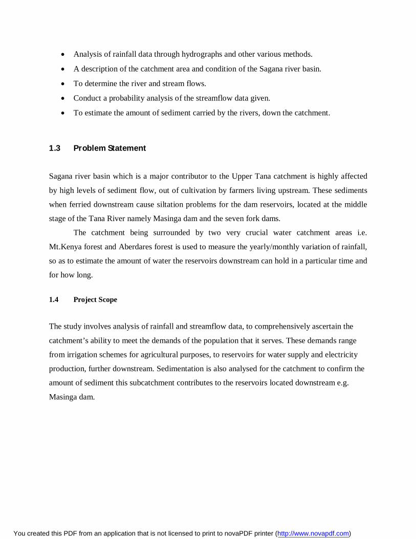
1.3 Problem Statement

Sagana river basin which is a major contributor to the Upper Tana catchment is highly affected

by high levels of sediment flow, out of cultivation by farmers living upstream. These sediments

when ferried downstream cause siltation problems for the dam reservoirs, located at the middle

stage of the Tana River namely Masinga dam and the seven fork dams.

The catchment being surrounded by two very crucial water catchment areas i.e.

Mt.Kenya forest and Aberdares forest is used to measure the yearly/monthly variation of rainfall,

so as to estimate the amount of water the reservoirs downstream can hold in a particular time and

for how long.

1.4 Project Scope The study involves analysis of rainfall and streamflow data, to comprehensively ascertain the

catchment’s ability to meet the demands of the population that it serves. These demands range

from irrigation schemes for agricultural purposes, to reservoirs for water supply and electricity

production, further downstream. Sedimentation is also analysed for the catchment to confirm the

amount of sediment this subcatchment contributes to the reservoirs located downstream e.g.

Masinga dam.



Chapter Two

Literature Review

2.1 Sagana Catchment Descriptions

Sagana (4A) catchment is bounded by latitudes 0o1’7.5’’ to 0o37’30’’ South and Longitudes

36o37’30’’ to 37o15’ East. It runs from the Aberdares in the west, extending eastwards to

Mt.Kenya. The catchment area covers an area of 2738 km2, with an estimated population of

around a million people.

The elevation of the catchment ranges from 1600m above sea level (asl) at the mouth of

river sagana at the catchment, to 3400m asl at the foot of the Aberdares, and 4000m at the foot of

Mt.Kenya.

Map 2.0 Showing the 4A catchment boundaries, rivers, River Gauging stations and contours.



2.1.1 Economic Activities of Inhabitants

The main occupation of the people living within the catchment is farming, mainly of cash crops

like coffee, tea and many more.

The other economic activities of the region being very near to tourism sites like

Mt.Kenya and Aberdares is hospitality industry, with installments such as the sagana state lodge,

treetops hotel and the sagana river camping , water rafting and bungee jumping.

Nyeri town also located within the catchment is a relatively big urban centre, where the

former central province headquarters were located, and is thus its urban lifestyle setting is much

like you would find in any town, its size in Kenya.

Agriculture is the main economic activity of the people living within the catchment area,

mainly due to the rich red soils and high amount of rainfall. Even the urban centres located in the

catchment thrive on agricultural productivity.

More intensive agriculture is done at mid-elevations and a huge array of crops are grown

including tea, coffee, maize, bananas, and beans.

Plate 2.0 Showing the main economic activity of inhabitants of 4A catchment: Agriculture



2.1.2 Developments around the Catchment

Out of the agricultural productivity of the catchment’s soils and the flat topography down the

catchment in Kirinyaga, Mwea-tebere irrigation scheme is one of the developments that are

notable. The main crop grown in the irrigation scheme is rice mainly for sale to the local market.

Even with high rainfall at altitudes higher than 1,800 m, there is a noted seasonal

variation in river flow. During these dry periods, high demand for water both for irrigation and

urban needs as well as sustained electric power generation cannot be adequately met. Due to this

seasonal fluctuation in river flows, the Masinga Dam was constructed.

Though the dam is located out of this catchment, the contribution it makes is

considerable. It’s noteworthy that most studies dealing with the dam’s capacity have to include

the whole upper Tana (4) catchment of which the Sagana is part of. The dam regulates the flow

of water to the downstream reservoirs (Kamburu, Gitaru, Kindaruma and Kiambere) and serves

as a water supply for the surrounding areas. (R. Arthurton et al, 2009)

2.2 Catchment Climatology and Hydrology

With the catchment sandwiched between two water towers, the climate is generally cold and wet. This climate is conducive to growth of certain cash crops like tea and coffee which thrive best under such conditions. There are two distinct rainy seasons in the catchment: March-April-May (long rains) and October-November (the short rains).

The daily temperatures range from 10°C to 20oC, with the coldest points being near to the water towers and the warmest being at the mouth of the catchment.

2.2.1 Streamflow

The 4A catchment has fairly well distributed network of river gauging stations which are crucial in getting data which is non-biased in statistical analysis. However, some rivers are overserved with Chania river having two river gauging stations i.e. RGS 4AC05 and RGS 4AC4, while other lack a recording station altogether.



Below is a list of the major stations whose data was availed for this project.

Gauge ID River Name Longitude Latitude Years of Record 4AA01 ------- 37o 03’44’’E 0o 21’16’’S 1947-1992 4AA04 ------- 36o 58’08’’E 0o 20’38’’S 1949-1998 4A B05 Amboni 36o 59’20’’E 0o 21’ 00’’S 1949-1996 4A C03 Sagana 37o 02’35’’E 0o 26’57’’S 1948-1999 4AC04 ------- 36o 57’12’’E 0o 25’56’’S 1952-1988 4A D01 Gura 37o 04’35’’E 0o 31’02’’S 1951-1996 4AC05 Chania 36o 47’28’’E 0o 25’55’’S 1959-1998

Table 2.0 Streamflow stations

2.2.1.1 Streamflow Measurement

Calculation of the discharge passing through a river’s cross-section is done by multiplying the

average velocity of the cross-section with its area (approximated as a trapezium). The velocity is

measured with a current meter which dipped in the flowing water to a distance of 0.6 times the

depth of water at that point, since the velocity at this point is seen to represent the average

velocity well for most streams. There are many different types of current meters, of which the

Price cup-type current meter attached to a round wading. (Calver et al, 2005)

Fig 2.1. Showing a horizontal axis currentmeter

Current meters are velocity measuring devices that that are used to measure the velocity

of a stream at a point. Each point velocity measurement is then assigned to a meaningful part of

the entire cross section passing flow. Several classes of current meters are used in water

measurement.



o Anemometer and propeller velocity meter

o Electromagnetic velocity meters

o Doppler velocity meters

o Optical strobe velocity meters

2.2.1.2 Flow Variation across a River Cross-Section

Stream discharge data used in this study were from the Thego, Amboni, Sagana, Gura, Sagana,

gauging stations located on their respective river tributaries. Though the amount of discharge

flowing through the river is of interest to a water resources engineer, it cannot be measured

directly by any instruments.

Rather, an indirect method is used which requires knowledge of the velocity distribution

in a river or an open channel. It may be observed that velocity is highest at the center of the river

but is zero at the banks. If a velocity profile were plotted on another horizontal plane at certain

depth of the river, the velocity profile would be found to be of a certain shape. (O,Connell et

al,2005)

Similarly the velocity profile of the river flowing in flood would be as shown in Figure

2.2, showing that the velocities over the flood plains is smaller compared to the main stream

flow.

In order to measure the discharge being conveyed in a river, the velocity profile or the

average velocity at a number of equally spaced sections are measured, as in Figure 2.2. The total

discharge is then approximately taken equal to the sum of the discharges passing through each

segment. The water level in a river varies, causing a proportional change in the total discharge

conveyed.

For each point of a river, the relation between stage and discharge is unique but a general

form is found. It may be interpreted from Figure 2.2 that the velocity in a river cross section

actually varies from bank to bank and from riverbed to free water surface and hence, can be

called a two dimensional variation in a vertical plane.



Fig 2.2 Shows the velocity profile across the cross-section of a river. 2.2.1.3 Flow Variation along A River Length For engineering purposes it is, sufficient, generally, to use an equivalent velocity in the direction

of river motion (perpendicular to river cross section) which may be obtained by dividing the total

discharge by the cross sectional area.

In a natural river, therefore, these flow velocities may vary from section to section there

are quite a few examples of non-uniform flow in rivers or open channels that may be

encountered by a water resources engineer. A compound section may be defined as a section in

which various portions of the cross-section have different flow properties, like surface roughness

or channel depth for problems concerning the steady uniform flow in rivers and open channels,

the manning’s equation is commonly used world over.

The depth of water corresponding to a discharge in a channel or river under uniform flow

conditions is called “normal depth” since the cross section, bed slope and flow resistance vary

along a river length, the depth and velocity would vary correspondingly. However, if a short

stretch of a river section is taken, then the variations in riverbed, water surface and the total

energy may be considered as linear. (Baylist et al, 2001)



Plate 2.1 Above is a typical streamflow station located along Sagana River

2.2.1.4 Flood Frequency

It must be appreciated that a minimum flow in the rivers and streams, even during the low

rainfall periods is essential to maintain the ecology of the river and its surrounding as well as the

demands of the inhabitants located on the downstream.

It is a fact that excessive and indiscriminate withdrawal of water has been the cause of

drying up of many hill streams. It is essential that the decision makers on water usage should

ensure that the present usage should not be at the cost of a future sacrifice.

If the river is perennial, and the minimum flow of the river is sufficient to cater to the

flow through the canal, this arrangement is perfectly fine to irrigate a command area using a

barrage and an irrigation canal system.

However, if the river is non-perennial, or the minimum flow of the river is less than the

canal water demand, then a dam may be constructed at a suitable upstream location of the river.

This would be useful in storing larger volumes, especially the flood water, of water which may

be released gradually during the low-flow months of the river. (Lamb et al, 2005)



2.2.1.5 Low Flow Analysis

Typically, water levels are recorded at 15-minute intervals from which a mean flow can be

calculated for each day.

Persistent lack of rainfall or low rainfall in most parts of the country is the main cause of low

flows in rivers. Possible consequences of low flow are shifting of river courses, denying

livelihood humans, livestock and wildlife along the old river course.

Irrigation schemes however small are also affected by the low flows because normal water flow

moves aside from intake points.

Also water sources from the interior areas like pans and boreholes run short of water and not

much yield can be gotten from them.

Low flow conditions in rivers and streams are of fundamental importance to the ecological status

of the watercourse.

Any change in the seasonal pattern of flows, for example due to exploitation of

a groundwater source or abstraction of water from the river, may lead to irreversible changes to

the stream ecology. (Kjeldsen et al,2008)

Low flow analysis is also important when considering the construction of works in rivers and

streams (for example, a weir), and for river restoration schemes for which an understanding of

hydrological variation is important in determining appropriate restoration works.

2.2.1.6 Flow Hydrograph Characteristics of Sagana

Theoretically a dam constructed to reduce a flood peak should require the maximum possible

stream flow hydrograph. Hydrograph and the catchment’s characteristics the shape of the

hydrograph depends on the characteristics of the catchment. The major factors are listed below.

1. Shape of the Catchment

A catchment that is shaped in the form of a pear, with the narrow end towards the upstream and

the broader end nearer the catchment outlet shall have a hydrograph that is fast rising and has a

rather concentrated high peak.



A catchment with the same area but shaped with its narrow end towards the outlet has a

hydrograph that is slow rising and with a somewhat lower peak for the same amount of rainfall.

Though the volume of water that passes through the outlets of both the catchments is same (as

areas and effective rainfall have been assumed same), the peak in case of the latter is attenuated.

2. Size of the Catchment Naturally, the volume of runoff expected for a given rainfall input would be proportional to the

size of the catchment. But this apart, the response characteristics of large catchment (say, a large

river basin) is found to be significantly different from a small catchment (like agricultural plot)

due to the relative importance of the different phases of for these two catchments.

Further, it can be shown from the mathematical calculations of surface runoff on two

impervious catchments (like urban areas, where infiltration becomes negligible), that the non-

linearity between rainfall and runoff becomes perceptible for smaller catchments.

3. Slope

Slope of the main stream cutting across the catchment and that of the valley sides or general land slope affects the shape of the hydrograph. Larger slopes generate more velocity than smaller slopes and hence can dispose of runoff faster. Hence, for smaller slopes, the balance between rainfall input and the runoff rate gets stored temporally over the area and is able to drain out gradually over time. Hence, for the same rainfall input to two catchments of the same area but with different slopes, the one with a steeper slope would generate a hydrograph with steeper rising and falling limits. A similar amount of rainfall over a flatter catchment produces a slow-rising moderated hydrograph than that produced by the steeper catchment.

2.2.1.7 Flow Duration Curves

A flow duration curve (FDC) represents the relationship between the magnitude and duration of

stream flows; duration in this context refers to the overall percentage of time that a particular

flow is exceeded.

The shape of the FDC for any river therefore strongly reflects the type of flow regime and is

influenced by the character of the upstream catchment including geology, urbanization, artificial

influences and groundwater.



The FDC is a very useful tool for assessing the overall historical variation in flow, though one

drawback is that it offers little information about the timing or persistence of low flow events.

The FDC has a wide range of applications including:

setting river flow objectives;

scenario evaluation (in respect of the impact of artificial influences such as water abstraction

or effluent releases);

hydropower assessment;

evaluation of sediment or contaminant loads;

structure design (for example, a structure can be designed to perform well within some range

of flows, such as those exceeded between 20 and 80% of the time or such that it does not

alter the low flow regime).

The accuracy of high flow records has a direct impact on the accuracy of flood estimation. It is

therefore essential to understand how flow is measured at a gauging station and the likely limits

in accuracy of high flows.

2.2.2 Rainfall

The mean monthly rainfall at a place is determined by averaging the monthly total rainfall for

several consecutive years. Rainfall follows a similar elevation gradient as that of soils. Mt.

Kenya and the Aberdare Ranges receive greater than 1,800 mm/yr of rainfall. At the mid

elevations (1,200 to 1,800 m) where intensive agriculture is predominant, annual rainfall ranges

from 1,000 to 1,800 mm/yr.

The mean annual rainfall is primarily dependent upon distance from the ocean (or a large water

body e.g. a lake), direction of the prevailing winds, the mean annual temperature, altitude of the

catchment, and the catchment’s topography. Closeness to the lake gives Lake Victoria basin high

rainfall amounts but it’s the mean annual temperature, altitude and catchment’s topography that

gives the Sagana catchment its characteristic high rainfall amounts.

The catchment is characterized by a third quarter that’s wet and cold during the month of July

with low rainfall amounts and dry spell in the months of august to September. It can also be said



that the months of March to May receive the highest amount of rainfall in a year and are called

the long rains, while the months of October and November are characterized with quite a huge

amount of rainfall but which does not exceed the long rain amounts, thus called the short rains.

Out of the rainfall data, it’s evident that rainfall stations that are closest to the two water towers

receive huge amounts of rainfall.

Also evident from the rainfall station distribution across the catchment is that most stations are

located near and around Nyeri town. This may be explained by the ease of getting around town

due to good roads; however there are fewer stations near the water towers out of the

impassability of the forests surrounding them.

2.2.2.1 Measurement of Rainfall

Rainfall may be measured by a network of rain gauges which may either be of non-recording or recording type.

This recording type rain gauge has an automatic mechanical arrangement consisting of

clockwork, a drum with a graph paper fixed around it and a pencil point, which draws the mass

curve of rainfall. From this mass curve, the depth of rainfall in a given time, the rate or intensity

of rainfall at any instant during a storm, time of onset and cessation of rainfall, can be

determined. The gauge is installed on a concrete or masonry platform 45 cm square in the

observatory enclosure by the side of the ordinary rain gauge at a distance of 2-3 m from it.

The gauge is so installed that the rim of the funnel is horizontal and at a height of exactly

75 cm above ground surface. The self-recording rain gauge is generally used in conjunction with

an ordinary rain gauge exposed close by, for use as standard, by means of which the readings of

the recording rain gauge can be checked and if necessary adjusted.

There are three types of recording rain gauges—tipping bucket gauge, weighing gauge

and float gauge, with the tipping bucket rain gauge being the most common of them all.



2.2.2.2 Rain-Gauge Density

For a scientific study of a catchment to be possible, there are certain thresholds pertaining to the

amount of raingauge presents and their subsequent density in the catchment.

While for a developed country the density is about one station per 100km2, and that for

most developing countries is about one station per 500km2, Kenya’s station density varies mainly

due to the nations varying climatic conditions i.e. catchments that have high rainfall amounts like

the lake Victoria basin and the Mount. Kenya basins have a very high density of rainfall gauge

stations, with an average of a one station per 150km2. But other low yield catchments like the

Athi river catchment and the ewaso nyiro catchment have station density that’s too low.

This is partly because the former have been identified for water and power projects

crucial to the nation’s survival, and thus most resources and research in the relevant ministries

have been channeled to further the cause of national productivity.

2.2.2.3 Duration of Recording

The length of record (i.e., the number of years) required to obtain a stable frequency distribution

of rainfall is recommended as below. For catchments that are an Island shore, plain ones, and

mountainous ones the best length of time is 30, 40 and 50 years respectively.

The Sagana (4A) Catchment, borders two mountains – Aberdare Ranges and Mount.

Kenya is obviously very mountainous and it’s required to have at least 50 years of rainfall

records.

Rainfall measurement is commonly used to estimate the amount of water falling over the

land surface, part of which infiltrates into the soil and part of which flows down to a stream or

river. For a scientific study of the hydrologic cycle, a correlation is sought, between the amount

of water falling within a catchment, the portion of which that adds to the ground water and the

part that appears as streamflow. Some of the water that has fallen would evaporate or be

extracted from the ground by plants. The time of rainfall record can vary and may typically range

from 1 minute to 1 day for non – recording gauges, Recording gauges, on the other hand,

continuously record the rainfall and may do so from 1 day 1 week, depending on the make of

instrument.



The rainfall stations in the catchment and their detail are as below. STATION ID STATION NAME LONGITUDE LATITUDE Years of Record 9036251 Nyeri forest station 0 o 20`S 36o 56È 1992-1995 9036269 Gatarakwa chiefs office 0 o 17`S 36 o 43È 1992-2003 9036271 Kiandongoro gate 0 o 29`S 36 o 45È 1992-1999 9036273 Ruhuruini gate 0 o 23`S 36 o 38È 1992-1999 9036274 Treetops gate 0 o 21`S 36 o 54È 1992-1999 9036275 Mweiga HQ 0 o 20`S 36 o 55È 1992-1999 9036282 Nyeri hill 0 o 25`S 36 o 54È 1992-1996 9036288 Nyeri metereological station 0 o 27`S 36 o 56È 1992-2013 9036316 Nyeri Baptist high school 0 o 25`S 36 o 58È 1992-1993 9037126 Kagumo high school 0 o 24`S 37 o 01È 1992-1997 9037138 Naromoru forest station 0 o 12`S 37 o 07È 1992-1997 9037139 Naromoru settlement scheme 0 o 12`S 37 o 04È 2004-2009 9037158 Sagana state lodge 0 o 22`S 37 o 04È 1992-2005

Table 2.1 Rainfall stations

2.2.2.4 Mean Rainfall

This is the average or representative rainfall at a place. The mean annual rainfall is determined

by averaging the total rainfall of several consecutive years at a place. Since the annual rainfall

varies at the station over the years, a record number of years are required to get a correct

estimate.

2.2.2.5Analysis for Anomalous Rainfall Records

Rainfall recorded at various rain gauges within a catchment should be monitored regularly for

any anomalies. For example of a number of recording rain gauges located nearby, one may have

stopped functioning at a certain point of time, thus breaking the record of the gauge from that

time onwards.

Sometimes, a perfectly working recording rain gauge might have been shifted to a neighborhood

location, causing a different trend in the recorded rainfall compared to the past data. Such

difference in trend of recorded rainfall can also be brought about by a change in its location or a

change in the ecosystem, etc. These two major types of anomalies in rainfall are categorized as

Missing rainfall record

Inconsistency in rainfall record



1. Missing Rainfall Record

The rainfall record at a certain station may become discontinued due to operational reasons. One

way of approximating the missing rainfall record would be using the records of the rain gauge

stations closest to the affected station by the law of averages.

For statistical analysis of rainfall data a sufficiently long record is required. It may so happen that

a particular rain-gauge is not operative for a certain period of time – being broken or otherwise.

This necessitates the need to supplement the missing records by the methods mentioned below.

Station-year method—In this method, the records of two or more stations are combined into one

long record provided station records are independent and the areas in which the stations are

located are climatologically the same. The missing record at a station in a particular year may be

found by the ratio of averages or by graphical comparison.

By simple proportion (normal ratio method)

2. Inconsistency in Rainfall Record

This may arise due to change in location of rain gauge, its degree of exposure to rainfall or

change in instrument, etc. The consistency check for a rainfall record is done by comparing the

accumulated annual (or seasonal) precipitation of the suspected station with that of a standard or

reference station using a double mass curve.

The trend of the rainfall records at a station may slightly change after some years due to a

change in the environment (exposure) of a station either due to coming of a new building, fence,

planting of trees or cutting of forest nearby, which affect the catch of the gauge due to change in

the wind pattern or exposure. The consistency of records at the station in question is tested by a

double mass curve by plotting the cumulative annual rainfall at the station against the concurrent

cumulative values of mean annual rainfall for a group of surrounding stations, for the number of

years of record.

From the plot, the year in which a change environment has occurred is indicated by the

change in slope of the straight line plot. The rainfall records of the station under review are



adjusted by multiplying the recorded values of rainfall by the ratio of slopes of the straight lines

before and after change in environment.

2.2.3 Sedimentation

Sediment concentration in rivers across the catchment varies seasonally and is therefore the

concentration of the sediment is measured in different rivers or even the same river at different

locations depending on the status of river sub catchments and human activities taking place in

the proximity of the rivers and within the rivers.

Sedimentation occurs due to the result of two processes namely erosion of soil and the

transport of the eroded soil (sediment) by water. The erosion of soil is mainly due to rain and

flowing water. The rain dislodges soil particles out of their fixed position, making them easy to

be carried away by elements of nature like wind, animals and more relevantly flowing water.

Factors known to aggravate sediment input in rivers were such as deforestation, removal

of vegetation cover, poor land use practices, domestic sewage and industrial waste discharges,

sand harvesting in rivers and sediment input from cultivated riverside areas and irrigated fields.

Suspended sediment concentration is usually highest during rainy periods and as rains subside

and vanish, most sediment settles, improving the clarity of the rivers.

Sedimentation is particularly prevalent during the rainy seasons when the Sagana

overflows its banks and temporarily floods the plains. (Ministry of water, 2010)

Surface runoff in the ephemeral streams feeding the draft reservoir from the sides also

contributes to sedimentation. The high production rates of sediment can be linked with the fact

that these rivers pass through the intensively cultivated slopes of the Aberdares and Mt. Kenya.

Lack of adequate ground cover and steep slopes (often cultivated without carrying out

effective soil conservation measures) result in increased surface runoff and soil loss. Thus, soil

conservation practices such as channel stabilization, road ditch stabilization terraces and

construction of check-dams should be carried out within the catchment.

Since Masinga reservoir has high trap efficiency (between 75 and 98%), with a mean

annual loss of capacity of 23 mm3, complete siltation of the reservoir would occur within



65years, as opposed to the original 500 year estimate, without some type of intervention and

management. Reforestation is thus explored as a means of addressing siltation issues in the

reservoir. (Brown et al, 1996)

2.2.3.1 Sediment Measurement

Measurement of sediment loads is done in three segments i.e. bed load measurements, suspended

load measurements, and total load measurements.

Bed load samples are taken from bed load flow region which is located 10 – 20 cm above

the channel bed. For small rivers samples are obtained by pumping from this region but for

larger rivers a scoop type of sample is used. The scoop is placed at the channel bed and left there

for sometime interval for the sediment to collect inside after which the scoop is then removed

and the accumulated sediment measured.

The sediment load measured is expressed in parts per million (ppm) or mg/l.

Out of the non-uniformity of flow or movement of dunes along the channel bed, there is usually

a difficulty in obtaining samples from the channel bed.

For suspended load measurements two samplers namely the point integrating samplers

and the depth integrating samplers are used. The sampler is kept at different points of the channel

depth to obtain the sediment concentration at each depth. The depth sampler is lowered into the

water and then lifted up as its design allows it to let sediment inflow at a constant rate. It then

gives an average sediment concentration along the channel bed straight away.



Plate 2.2 A MoW employee collecting water sediment samples. (MoW, 2012)

2.2.3.2 Errors in Sediment Measurement

It’s often difficult for a sampler to take a correct vertical and horizontal alignment vis-à-vis the

direction of motion of river and sediment flow.

Hardly is there any bed load sampler that can collect all sizes of sediments of the bed

load. The portion of the actual bed load caught by a sampler is influenced by the type of sampler

used and the relation between the geometry of the sampler and the size and geometry of the bed

form.

Accuracy of the bed load measurements by using radio-active tracers is affected by the

amount of background concentration of the tracer in the stream and the degree of mixing of the

tracer with the sediments between the point of introduction and point of sampling.

The sampler’s presence itself is sufficient to disturb the flow pattern and as such the intensity of

sediment concentration is not correctly gotten. (Odira, 2013)



Suspended load measurement’s accuracy is also affected by a host of logistic factors

which include verticals having maximum and minimum concentrations in a cross-section change

position with time; also the verticals in a cross-section for maximum concentration of different

size ranges may not coincide; suspended load samplers do not traverse a region of about 10cm

above the channel bed; experimental evidence also suggests that the standard deviation of the

depth integrated suspended load concentration at a vertical may be 10% or more of the mean.

(Odira, 2013)

2.3 Catchment degradation

The biggest threat to the sagana river catchment is deforestation of the forests surrounding the

two main water towers namely Mt.Kenya forest and the Aberdares. This threat is so real that the

ministry of water raised the alarm in 1990’s about the Aberdares, which the government

responded by evicting people who had encroached into the forest and finally fenced it.

These forests are also under extreme threats emanating from charcoal production,

overgrazing, extensive illegal logging of indigenous tree species, abuse of the Shamba-system

and additional encroachment from such practices as large-scale marijuana cultivation. (R.

Arthurton et al, 2009)

High population density in these areas is a cause of over-abstraction, both of ground and

surface water. These people also involve themselves in farming practices that contribute to a lot

of sedimentation that in turn affect the dams and irrigation schemes located downstream.

There’s quite a number of agro-based industries and urbanization which contribute to

substantial pollution to the water resources e.g. Coffee and tea factories which are located along

the rivers for feeding fermentation tanks.

However land use practices such as terracing, strip cropping, contour ploughing all to

reduce erosion, check dams in gullies to retain some sediment and reduce sediment flow into



stream and finally a vegetative cover to reduce the impact force of raindrops and minimize

erosion.

Plate 2.3 Showing the amount of deforestation and land clearing for agriculture along

River Sagana



CHAPTER THREE

METHODOLOGY AND RESULTS

This involves the description of the methods used in collection of data that will be used in the

analysis of the subject matter. The methods used here are described as per the category of data

type e.g. rainfall data, streamflow data and so on.

I also find it necessary to attach a section of the raw data in the methodology, so as to

have a good comparison in the analysis part especially as pertains filling missing data.

3.1 RAINFALL DATA

Due to the nature of this project, the amount of data required for a satisfactory analysis was huge.

Therefore the most resourceful departments, were government departments mainly the

meteorological department at Dagoretti corner, and the ministry of water at NHIF building in

Upperhill, Nairobi.

The station ID’s are first identified for the relevant catchment – in this case 4A

catchment, from which the relevant data on rainfall is classified and given out. There is however

restrictions on the amount of data that can be given out to anyone, thus limiting the range of data

that I had planned on using for analysis.

For example the sagana-4A catchment has well about 30 stations but the meteorological

department could only surrender data for 20 of these.

They include chinga boys high school, Nyeri forest station, kiambuthia secondary school,

gatarakwa chief’s office, kiandongoro gate-aberdare N.park, Ruhuruini gate- Aberdares N.park,

treetops gate – Aberdares N.park, mweiga HQ – Mt.Kenya national park, Nyeri hill, Nyeri

meterological station, ngethu water supply, Nyeri Baptist high school, wanjerere forest station,

kagumo high school – kiganjo, naromoru forest station, naromoru settlement scheme, sagana



state lodge, ngorano chief’s camp – karatina, upper naromoru forest post, kiaraho primary

school.

The met department also surrendered the data for Todenyang police post (Station ID:8535001)

but which later came out as out of the catchment, and its analysis dismissed.

3.1.1 Filling Missing Data

For comparison, a ministry of water, handbook is used to fill and confirm the figures given by

met department. This is to ensure the data used in analysis is consistent as per statistical

requirements. Filling data involves using the law of averages severally to estimate the amount of

rainfall a certain spot is missing. It may have its uncertainties but it’s the closest to the real data

that any method of estimation can get.

Once the missing data is filled, the monthly means and annual means were computed for

each station and each year, respectively the stations were operational. The monthly means were

put horizontally below each station, while the annual means were arranged vertically alongside

the various years of operation of the various stations.

3.1.2 Bar Graphs

Bar graphs showing seasonal variation of the catchment was done for two stations ie Nyeri

metereological station and kiandongoro gate – Aberdares N.Park. One station is near a

moderately populated area in an urban centre, while the other is near the Aberdares forest- a very

important water tower.



3.1.3 Catchment’s Mean Rainfall Calculation

A catchment’s mean monthly/annual rainfall can be calculated using two methods namely

Thiessen polygon method and the Isohyetal method. The latter is deemed more accurate but both

have been used to estimate the mean for comparison purposes too.

3.1.3.1 Thiessen Polygon

This method involves allocating an influence area to a rainfall station. This is accomplished by

joining adjacent stations using a single line, to form convenient triangles, which are replicated till

all stations both in and out of the catchment form a network of adjoining lines.

Perpendicular bisectors of the lines joining each station to the other are then drawn, and

made to join each other to surround a rainfall station with a polygon. The area of this polygon is

what constitutes the influence area of the station. The product of the rainfall depth of each station

with their influence areas is cumulatively added, with that of other stations. The sum of these

products is then divided by the total area of the catchment, to obtain the mean monthly/annual

rainfall of the catchment. (IIT Kharagpur, 2008)

3.1.3.2 Isohyetal Method

Isohyetal method tends to use the difference in rainfall depths throughout the catchment to generate the mean monthly/annual rainfall.

The mean rainfall of a catchment is noted beside the rainfall station’s location, and the areas of equal rainfall depth marked with a line traversing through the entire catchment. All areas of the catchment have to have a rainfall depth (isohyet) allocated to them. The area between the various isohyets is then gotten and multiplied with the average rainfall depth of an isohyet. The area of a catchment tip – not between any two isohyets is assumed to have the rainfall depth of the last isohyet.

To get the mean monthly/annual rainfall, the cumulative product of rainfall depth and area between isohyets is divided with the area of the catchment. (IIT Kharagpur, 2008)



3.1.3.3 Arithmetic Mean Method

The simplest of all is the Arithmetic Mean Method, which is gotten from finding the average of the stations without any complexities involving influence areas.

3.2 STREAMFLOW DATA

Streamflow data was obtained from the ministry of water. The ministry through its various

grassroots officers, records daily data of river flow by use of the various River gauging stations

installed along the rivers. At most sites, flow is assessed by measuring the water level and

converting it to discharge using a rating curve.

Rating curves are prone to uncertainty due to extrapolation and because many gauging

stations are bypassed in flood conditions; this uncertainty is often far greater at flood flows than

at low to medium flows. Thus this daily data per river gauging station (RGS) is tabulated per

station for all the years of the station has been in operation.

3.2.1 Filling Missing Data

Just like all tabulated data over a long period of time, there are gaps that need to be filled to be

able to perform statistical analysis of the data. Like earlier stated doing averages of the station

data surrounding the missing one is the most common way of solving this problem.

3.2.2 Calculating Monthly Mean, Maximum, Minimum

Once the missing data is filled, analysis of the monthly average, total, maximum and minimum is

done. The derivatives are put at the side of the raw data as is the norm. These statistics are very

crucial in making deductions about the suitability of erecting a dam, putting up an irrigation

scheme, or just plain analysis of possibilities of drought or flood in a particular area.



3.2.3 Flow Hydrograph

If data from one station is picked, and its annual mean stream flow data plotted against the

corresponding years [x-axis], then the resulting diagram is a flow hydrograph. It’s very essential

in picking out the flood years and the drought years in the catchment or along a river.

3.2.4 Flow Duration Curve

Once mean monthly data is obtained as described above, the data is ranked. Ranking involves

arranging the data in ascending or descending order, then putting the data in classes. The tally of

each class is made against it, followed by a frequency tabulation of the various classes.

The cumulative frequency (n) is then filled categorically. The midpoints of the various classes

are also calculated. The probability curve is a graph of class mid-points against their probabilities

in a probability paper where the mid-point scale is logarithmic while the probability scale is

probabilistic.

To obtain the probability column is obtained as follows:

Probability= [풏 풎 + ퟏ]

Where n is the cumulative frequency of a particular class

m is the total frequency

A flow duration curve (FDC) represents the relationship between the magnitude and duration of

stream flows; duration in this context refers to the overall percentage of time that a particular

flow is exceeded. The shape of the FDC for any river therefore strongly reflects the type of flow

regime and is influenced by the character of the upstream catchment including geology,

urbanization, artificial influences and groundwater. (IIT Kharagpur, 2008)



3.2.4.1 Ranking Data

Data used in probability curves is put in predetermined classes which are as follows:

1 – 1.5, 1.5 – 2.0, 2.0 – 3.0, 3.0 – 4.0, 4.0 – 6.0, 6.0 – 8.0, 8.0 – 10.0 for the logarithmic cycle of

1 – 10.

For the logarithmic cycle of 10 – 100, it’s as follows:

10 – 15, 15 – 20, 20 – 30, 30 – 40, 40 – 60, 60 – 80, 80 – 100.

For the final logarithmic cycle between 100 – 1000, the divisions are as follows:

100 – 150, 150 – 200, 200 – 300, 300 – 400, 400 – 600, 600 – 800, 800 – 1000.

The above logarithmic classes are what were relevant for the data available; otherwise there exist

other logarithmic cycles both below and above the stated ones above.

3.2.4.2 Percentiles Necessary for Analysis

To obtain the mean streamflow for the particular station using the probability curve, the 50%

percentile is struck off and its corresponding midpoint noted down.

Other notable percentiles that are crucial for analysis include 95%, 98%, 99%, 99.5%.

3.2.5 Low Flow Analysis

Monthly mean flow data are useful to summarize overall water balance and yield for catchment,

or low flow analysis. For each year the minimum monthly mean flow for both stations under

study are used in a probability analysis of the data.

Monthly mean flow data is first arranged in ascending order and the resulting order is put

in classes (or ranked as shown in the notes above).

The tally is made to corresponding classes and the frequency noted alongside the respective

class. From the top, the frequency is added cumulatively down to the last class down the

arrangement and this deduction is followed with that of probability. (Calver et al, 2005)

Probability= [풏 풎 + ퟏ]

Where n is the cumulative frequency of a particular class

m is the total frequency



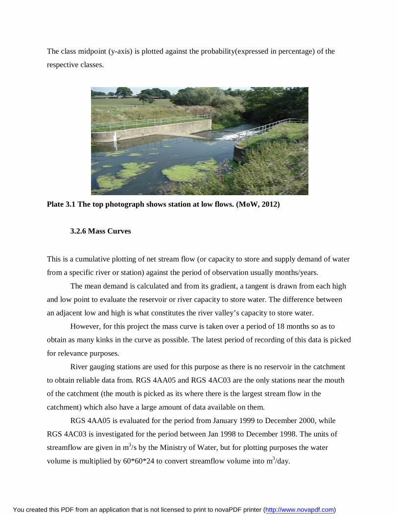
The class midpoint (y-axis) is plotted against the probability(expressed in percentage) of the

respective classes.

Plate 3.1 The top photograph shows station at low flows. (MoW, 2012)

3.2.6 Mass Curves

This is a cumulative plotting of net stream flow (or capacity to store and supply demand of water

from a specific river or station) against the period of observation usually months/years.

The mean demand is calculated and from its gradient, a tangent is drawn from each high

and low point to evaluate the reservoir or river capacity to store water. The difference between

an adjacent low and high is what constitutes the river valley’s capacity to store water.

However, for this project the mass curve is taken over a period of 18 months so as to

obtain as many kinks in the curve as possible. The latest period of recording of this data is picked

for relevance purposes.

River gauging stations are used for this purpose as there is no reservoir in the catchment

to obtain reliable data from. RGS 4AA05 and RGS 4AC03 are the only stations near the mouth

of the catchment (the mouth is picked as its where there is the largest stream flow in the

catchment) which also have a large amount of data available on them.

RGS 4AA05 is evaluated for the period from January 1999 to December 2000, while

RGS 4AC03 is investigated for the period between Jan 1998 to December 1998. The units of

streamflow are given in m3/s by the Ministry of Water, but for plotting purposes the water

volume is multiplied by 60*60*24 to convert streamflow volume into m3/day.



Assuming average water consumption per capita of 500 litres per day (taking care of even all

users and uses i.e. urban and rural, drinking, irrigation and power generation purposes), the total

consumption of the population using the water assumed to be about a million is as follows.

푇표푡푎푙푑푎푖푙푦푤푎푡푒푟푑푒푚푎푛푑 = 푝푒푟푐푎푝푖푡푎푐표푛푠푢푚푝푡푖표푛 × 푝표푝푢푙푎푡푖표푛푠푒푟푣푒푑

= 500푙푖푡푟푒푠/푑푎푦 × 1,000,000

= 150,000,000푙푖푡푟푒푠/푑푎푦

푇표푡푎푙푚표푛푡ℎ푙푦푤푎푡푒푟푑푒푚푎푛푑 = 푡표푡푎푙푑푎푖푙푦푤푎푡푒푟푑푒푚푎푛푑 × 30

= 500,000,000 × 30푑푎푦푠1000푙푖푡푟푒푠

= 1,500,000푚 /푚표푛푡ℎ

The mean monthly demand is 500,000m3 is used to calculate the storage required while using the

mass curves. This is appropriate for RGS 4AC03 out of its small river volume. But station has a

total cumulative streamflow volume of 20.0*106 m3/day while the RGS 4AA05 has a total

cumulative streamflow volume of 90.0*106 m3/day. Thus the demand of the latter is factored by

a multiple of a similar difference.

Thus for the RGS 4AA05 a water demand of 3,000,000 m3/day is possible out of the sheer

volume of waters passing through it. Thus for the mass curve calculations of the later, the

demand is put up commensurate with the capacity to supply some more.



3.3 Sedimentation

Sedimentation data was obtained from the ministry of water at Maji house, Upperhill, Nairobi.

The data is classified according to the particular river gauging station (RGS) the sedimentation

samples were taken from.

In order to eventually obtain the relationship between discharge and sediment load, the

point of measurement was as much as possible selected at Regular River gauging stations where

historically, there is water discharge data. The sediment loads were then computed and mapped

to show areas of highest/lowest sedimentation rates.

3.3.1 Amount of sedimentation

The amount of sedimentation is usually expressed in tons/day. It’s the product of the rate of

streamflow (Q,m3/s) with the suspended solids amount (mg/l), which yields the amount of

sedimentation in grams per second. This is comfortably converted to tons per day as below:

푻풐풏풔풑풆풓풅풂풚 = [푮풓풂풎풔× ퟏퟎ ퟔ/ 퐬퐞퐜] ×ퟔퟎ × ퟔퟎ× ퟐퟒ



3.4 Challenges in Data Collection

Collection of hydro-meteorological hasn’t been very effective due to non-payment of weir

readers and general poor remuneration of Ministry employees.

Re-installation of non-operational stations has been a big hurdle getting over out of low

government funding of the concerned departments, which is also compounded by corruption

within these departments too.



3.5 Results

Below are the results and analysis of the area and mean rainfall of the catchment.

1. USING ARITHMETIC METHOD

STATIONS ANNUAL MEAN (M) mm *10-3 m

NAROMORU FOREST STATION 82.74 NAROMORU SETTLEMENT SCHEME

52.19

SAGANA STATE LODGE 66.12 KAGUMO HIGH SCHOOL 67.24 NYERI FOREST STATION 67.24 MWEIGA HQ 64.56 TREETOPS GATE 75.08 NYERI BAPTIST HIGH SCHOOL 62.47 NYERI METEREOLOGICAL STATION

79.4

NYERI HILL STATION 74.37 KIANDONGORO GATE 160.50 RUHURUINI GATE 121.4 GATARAKWA CHIEF’S OFFICE 72.49 TOTALS 1045.8

TABLE 3.1 Arithmetic method 푀푒푎푛푎푛푛푢푎푙푟푎푖푛푓푎푙푙 = 푇표푡푎푙푎푛푛푢푎푙푚푒푎푛

푁표. 표푓푠푡푎푡푖표푛푠

= 1045.813 = 80.45푚푚



2. THIESSEN POLYGON METHOD OF FINDING MEAN RAINFALL

STATIONS ANNUAL MEAN (M) mm *10-3 m

INFLUENCE AREA (A)Km2

*106 m2

PRODUCT OF(M)*(A) *103 m3

NAROMORU FOREST STATION

82.74 148.476 2,284.904

NAROMORU SETTLEMENT SCHEME

52.19 146.260 7,633.309

SAGANA STATE LODGE 66.12 175.069 11,575.562 KAGUMO HIGH SCHOOL 67.24 121.883 8,056.466 NYERI FOREST STATION 67.24 128.532 8,637.350 MWEIGA HQ 64.56 35.457 2,289.104 TREETOPS GATE 75.08 115.235 8,651.844 NYERI BAPTIST HIGH SCHOOL

62.47 70.914 4,432.125

NYERI METEREOLOGICAL STATION

79.4 239.335 19,003.199

NYERI HILL STATION 74.37 101.939 7,581.203 KIANDONGORO GATE 160.50 281.440 45,171.12 RUHURUINI GATE 121.4 26.593 3,228.026 GATARAKWA CHIEF’S OFFICE

72.49 35.457 2,570.278

TOTALS 1,626.591 141,114.490

TABLE 3.2 Thiessen Polygon Method

푀푒푎푛푎푛푛푢푎푙푟푎푖푛푓푎푙푙 = 푇표푡푎푙[푝푟표푑푢푐푡(푀 ∗ 퐴)]푇표푡푎푙푎푟푒푎

= 141,114.490 ∗ 101,626.591 ∗ 10

= 86.75푚푚



FINDING THE MEAN ANNUAL RAINFALL OF SAGANA (4A) CATCHMENT BY USE OF BOTH ISOHYETAL AND THIESSEN POLYGON METHODS.

3. ISOHYETAL METHOD OF FINDING MEAN RAINFALL

AREA CODE RAINFALL DEPTH (mm)* 10-3 m

ACTUAL AREA(km2)* 10-6 m2

R.DEPTH*AREA (m3)* 103 m3

1 50 24.377 1218.85 2 55 106.371 5850.405 3 80 86.427 6914.16 4 75 126.316 9473.700 5 65 394.460 25639.900 6 75 199.446 14958.450 7 85 135.180 11490.300 8 95 115.235 10,947.325 9 125 294.737 36842.125 10 150 110.803 16620.450 TOTALS 1,593.352 139,955.450

TABLE 3.3 Isohyetal Method

푴풆풂풏풂풏풏풖풂풍풓풂풊풏풇풂풍풍 = 푻풐풕풂풍[푹풂풊풏풇풂풍풍풅풆풑풕풉 ∗ 푨풓풆풂]푻풐풕풂풍[푨풓풆풂]

= ퟏퟑퟗ,ퟗퟓퟓ.ퟔퟔퟓ ∗ ퟏퟎퟑퟏ,ퟓퟗퟑ.ퟑퟓퟐ ∗ ퟏퟎퟑ

= ퟖퟕ.ퟖퟒ풎풎



Chapter Four

Discussion and Analysis

The main objective of the study is to analyse the rainfall and streamflow characteristics of the

Sagana river (4A) basin by use of flow hydrographs, low flow curves, rainfall probability curves,

and rainfall data bargraphs.

Investigating the capacity of the catchment, to at any one point store water by use of

appropriate mass curves and subsequent analysis of data obtained is also a major aim of this

project.

To estimate the amount of sediment carried by the rivers, down the catchment. A

description of the catchment area of the Sagana river basin follows shortly after as the deductions

are made out of the analysis below.

4.1 Rainfall Analysis and Discussion

The mean monthly and annual rainfalls are gotten by conventional methods of calculating

averages. The annual means are used in getting a rainfall probability curves while the mean

monthly means for a chosen station are used for getting bargraphs used in getting seasonal

variation of rainfall in the catchment.



4.1.1 Rainfall Patterns across the Catchment

The main objective of the study is to get rainfall characteristics of the catchment through use of

mean monthly rainfall data and Bargraphs.

From the Bargraphs in Kiambuthia rainfall station, Station ID: 9036254, the peak rainfall

is at April with a value of 431mm of rainfall. But there is another peak, not as high but with

considerable depth of rainfall of 316mm in the month of October.

For Nyeri meteorological station, Station ID: 9036288, peak rainfall occurs in the month

of May at a high of 170mm of rainfall with a second peak coming in, in the month of November

at a depth of 133mm.

Also apparent from the bargraphs is that there are two drought seasons in a year i.e. from

December through January to February. The second one is from June to September, usually a

cold season.

Since the sagana catchment is sandwiched by two important water towers, the choice of

picking Kiambuthia which is near the Aberdare Ranges, and the Nyeri meteorological station

which is near an urban centre is deliberate. Kiambuthia Rainfall station has a high of 431mm of

rainfall while Nyeri Met station has a high of 170mm, and a consequent mean monthly average

rainfall of 211.78mm and 79.4mm respectively. It’s found that the amount of rainfall near a

catchment is significantly higher than that near an urban centre.

The trend is consistent with other stations ie. Stations near the Aberdares like Wanjerere

forest station [9036330], Ruhuruini gate [9036273], Kiandongoro gate [9036271], and Ng’ethu

water supply [9036308] which average a monthly depth of 183.89mm, 121.40mm, 160.50mm,

132.62mm respectively. Stations near Nyeri Township like Nyeri Baptist high school [9036316],

Kagumo high school [9037126], and Sagana State lodge [9037158] which have rainfall depths of

62.47mm, 66.12mm, and 66.12mm respectively.



4.1.2 Area of the Catchment

While calculating the mean rainfall of the catchment using both Isohyetal method and Thiessen

polygon methods, the catchment area was found to be 1593.352 km2 and 1626.591 km2

respectively.

However the ministry’s catchment area is 2738 km2, which is a higher figure than the one

gotten in the calculations above. The difference could be attributed to lack of a map with a

definite scale e.g. 1:250,000 as the maps used for this project were computer generated by

software that used triangulation to give the map a scale.

Also errors in tracing the map from the printed map to the tracing paper could have

transferred errors, but possibly very small errors. To find the area of the map from the tracing

paper (as it’s translucent) a graph paper was placed below it. Using the method of complete and

incomplete squares, the maps count of both was made with both very small and very huge

incomplete squares being counted as half of a square.

This could also have been a source of error as the bigger squares could be significantly in

bigger numbers in the count, with the smaller incomplete squares being small in count leading to

a huge chunk of areas of out 85% of a square being counted as 50% of a square.

Finally the other reason for the discrepancy is the assumption in this calculation that the

catchment topography is plain flat. Could it be so, the area of the catchment gotten here would be

remotely near the actual value. However, the contours out of the catchment’s hilly and

mountainous terrain coupled with earth’s curvature – which was not taken care of in this project,

swung the catchments’ area of the actual value.

4.1.3 Mean Rainfall of the Catchment

Using the simplest method of mean rainfall depth calculation – arithmetic mean method, the

mean is gotten as 80.45mm, which is an annual average of 965.4mm.

The other methods used namely Isohyetal and the Thiessen polygon methods give the

following results: 87.84mm and 86.75mm respectively. This points to an annual average of

1054.08mm and 1041mm of rainfall, respectively.



However the annual average rainfall of the catchment by various government

commissioned studies is around 1800mm of rainfall. There’s a big discrepancy between the

calculated annual average and the correct one.

This can be due to the inconsistencies in data recorded in the various stations, with some

data looking clearly out of normalcy. This could also be due to the missing data having lost key

station data that could have been very crucial in enhancing the consistency of data used in the

study.



4.2 Streamflow Analysis

4.2.1 Flow Hydrograph

From the two stations under study in the flow hydrograph, it’s apparently clear that there were

peak flows in the years of 1951-1953, 1958, and 1998 at station 4AC03, while for station 4AA05

there was a spike in the years of 1951-1954, 1980. All this points to a flood in all of these years

which quite accurate given the el Niño rainfall of 1998 is the most memorable event in recent

history.

Sudden spikes which drop as quick are a pointer to a flood i.e. for RGS 4AC03 there is 1951,

1958 and 1980 for RGS 4AA05. Sustained streamflow spikes suggest a flood that stayed on for

quite a long period i.e. for RGS 4AC03 we have 1967 – 1969, 1978 – 1980. In RGS 4AA05

sustained rainfall levels are obtained in the years of 1980 – 1982 with the year 1983 a drought

year.

4.2.2 Flow Duration Curve

The 50, 95 97.5, 98 and 99 percentiles for the flow duration curves were obtained as follows:

PERCENTILES

CLASS MID POINT VALUE(m3/s)

STREAMFLOW STATIONS (RGS)

4AA05 4AC03

50% 38 4.9

90% 90 16.0

95% 105 22.5

99% 135 47.0

TABLE 4.3 Flow Duration Analysis

Thus the mean stream flow is 38 m3/s for RGS 4AA05 and 4.9 m3/s for RGS 4AC03. Otherwise

while accommodating a 10%, 5% and 1% percent error the above results are obtained. The 5%

error is commonly used for rural areas estimation of streamflow to allow for the high amounts of

infiltration of rainfall into the soil, while the 1% is used in urban areas where the amount of

infiltration is low due to the impermeability of pavements and buildings in towns and cities.



4.2.3 Mass Curve

The mass curves of RGS 4AA05 has 3 troughs that point to possible storage of a good amount of

water were there a reservoir to store the water. The mean monthly streamflow is 3.0 ×

10 푚 /푑푎푦. The first is on September 1999 with storage of 2.5× 10 푚 /푑푎푦, the second is on

March of 2000 with 9.5 × 10 푚 /푑푎푦 and the third has no flood season preceding it thus the

amount of storage needed cannot be estimated.

Thus the highest possible storage at RGS 4AA05could have been 9.5 × 10 푚 /푑푎푦.

For RGS 4AC03 only two troughs are noted. One is on September 1998 with a possible storage

of a massive 7.00 × 10 푚 /푑푎푦 and the other is on March of 1999 with the smallest kink of

8. 0 × 10 푚 /푑푎푦. The stations mean monthly streamflow is9.85 × 10 푚 /푑푎푦.

The extremely high yield in the year 1998 at RGS 4AC03 is attributable to the phenomenon

which occurred that year that caused great flooding called El Niño. Hydrologically, an El Niño is

followed by an el Niña (a period of drought) thus the small yield in the following year (1999) in

a supposedly long rain season. This drought extended to the short rains as there was no storage

water available on October – November rains, which is not the norm in a normal hydrology

calendar.



4.2.4 Low Flow Curve

PERCENTILES

CLASS MID POINT VALUE(m3/s)

STREAMFLOW STATIONS (RGS)

4AA05 4AC03

50% 22.5 2.25

90% 55.0 4.3

95% 74.0 4.7

99% 97.5 5.2

TABLE 4.1 Low Flow Analysis

On comparison with the data of the flow hydrograph above, it’s easy to find that the derivations

above have a lower value than those of the flow hydrograph. This partly confirms it’s a low flow

curve. The mean low flow for both stations are 22.5m3/s and 2.25 m3/s for RGS 4AA05 and

RGS 4AC03 respectively.

4.3 Sedimentation Analysis

It’s found that stations with the highest sediment load are Gura RGS 4AD01at 118.65tons/day,

Chania RGS 4AC05 at 198.74 tons/day and Sagana RGS 4AC03 at 154.24tons/day. It’s also

worthwhile to note that these stations have a big streamflow volume of 43.31m3/s, 40.85m3/s,

and 30.41m3/s respectively. Since these stations have sediment concentration that is average of

about 30 – 60 mg/l, it’s safe to assume that the sheer volume of these waters is the biggest cause

of high sediment loads.

Another important deduction about these stations with high sediment load is that they are

located at the mouth of the catchment. Their locations downstream are perhaps the reason why

they ferry so much volume of water, as other rivers drain into them. This means that the more

the volume of water carried by a river the greater the sediment load however inconsequential the

sediment concentration maybe.

This is true as rivers up the catchment record low sediment loads out of the low water

volume they hold. This includes, Mweiga RGS 4AB2 at 0.02 tons/day, Tunuku RGS 4AD05 at



0.12 tons/day, and Upper Sagana RGS 4AA7 at 0.2 tons/day. Their respective flow rates are

0.0127m3/s, 0.0527m3/s, and 1.1819m3/s.

It’s also wise to analyse the stations with a higher concentration of sediments irregardless

of their total sediment load. Stations with the highest concentration of suspended solids are

Mweiga RGS 4AB3 at 408 mg/l, Muringato RGS 4AC07 at 318 mg/l and Kagumo RGS 4AB08

at 170 mg/l, while the stations with the least concentration of sediments include Gura RGS

4AD04 at 8mg/l, Upper Sagana RGS 4AA07 at 2mg/l and Sagana RGS 4AA01 at 8mg/l.

This trend has one simple deduction: Stations in an area of high settlement experienced

high sediment concentration e.g. Kagumo and Mweiga while stations near the two water towers

e.g. Upper Sagana RGS 4AA07 and Gura RGS 4AD04 have the least sediment concentrations.

This is because the area near water towers is covered in thick forests and a lot of vegetation

which prevents the carrying down of loose particles of soils down a river when rain hits the

ground and water flows to the river valley.

However the converse is true for the other stations like Kagumo and Mweiga whose

settlement upon by populations have made it vulnerable to soil carrying forces of runoff water

down a river. This is due to agricultural practices of the populations living there whose small

scale farming practices allow for little innovation on measures to keep the slopes free of soil

dislodging agents.

According to a study done by a French consortium led by Egis Bceom International for the

Ministry of Regional Development Authorities, that concentrated on the sediment load on three

stations namely RGS 4AA1, RGS 4AA5 and RGS 4AC03 the sediment loads in tons/year were

2231, 18845 and 8405 respectively. But from this project’s computations, the sediment is in

tons/year 627.8, 4949.4 and 56297.6 for RGS 4AA1, RGS 4AA5 and RGS respectively.

Cumulatively the project’s sediment load is much higher than that of the French consortium,

indicating that the amount of sediment carried down by the rivers of this catchment stand to

jeopardize the developments downstream i.e. irrigation schemes and most importantly the

reservoirs.

These glaring anomalies may be attributed to the lack of good record keeping by the ministry of

water coupled with use of techniques that yield less than perfect results. It’s also worth noting

that missing data that isn’t collected, contributes somewhat to the discrepancies of the data as

some events that may contribute to above average sedimentation are left out.



Chapter five

Conclusions and Recommendations

5.1 Conclusions

In a year of an average station, it’s found that there are two rainfall peaks commonly referred to

as wet seasons in a year i.e. from March to May, and from October and November. The former

i.e. March to May is called the long rains, since its rainfall peaks are about 50% more than that of

the short rains later on, while the second wet season is the short rains which as by the Bargraphs

has less rainfall levels than the long rains and also lasts a shorter period.

It’s also evident that rainfall is much higher near the water towers as opposed to the urban

areas since Kiambuthia rainfall station which is near the Aberdares has a peak rainfall of 431 mm

and a monthly mean of 211.18 mm, whilst the Nyeri Meteorological station which is near Nyeri

town has a high of 170mm with a mean monthly rainfall of 79.4mm.

On streamflow it was found that RGS 4AC03 has a lot less water volume than RGS

4AA05 making the latter’s ability to meet demand of the population possible. Other flow

hydrograph percentile analysis also reveals the same trend. Hence the most appropriate place to

locate a reservoir were there such a consideration would be River Gauging Station 4AA05.

Flow hydrographs also point to sustained floods in the catchment, in the years between

1951 – 1953. This is because of a spike in the hydrographs for RGS 4AC03 from 1951 – 1953,

and for RGS 4AA05 from 1951 – 1954.

Sedimentation in RGS 4AA5 and RGS 4AC03 is cumulatively supposed to be 27250

tons/year (French consortium - Egis Bceom, 2011) but the results of this project being 61247.0

tons/year, point to a near tripling of sediment carried down and out of the catchment. This poses

a grave danger to the reservoirs located downstream.



5.2 Recommendations

More rainfall stations should be put up to be at par with developed nations, station density of one

station per 100km2.

Apart from rainfall stations, it’s found that river gauging stations are not installed in some

rivers while others have two stations. For better hydrological studies, it’s necessary to put up

river gauging stations in all rivers, and they be put at the most appropriate location.

It’s also necessary to train enough workers to maintain and record the data at these

stations more frequently. If this is done, the amount of missing data will be greatly reduced

therefore enhancing the accuracy of raw data collected by the ministry.

Facing the amount of sedimentation found above, its incumbent upon the government to

move quickly to encourage better farming practices e.g. Contour farming, whilst discouraging

deforestation, encroachment on forest reserves and farming too near river banks. These measures

are necessary to increase the productive life of capital investments located downstream e.g.

Masinga dam, Mwea-tabere Irrigation scheme and others.



References

Marshall, D C W and Bayliss A C, Flood estimation for small catchments, Hydrological report

J. Institute of Hydrology.

O’Connell, P E, Beven, K J, Carney, J N, Clements, R O, Ewen, J, Fowler, H, Harris, G L,

Hollis, J, Morris, J, O'Donnell, G M, Packman, J C, Parkin, A, Quinn, P F, Rose, S C, Shepherd,

M and Tellier, S (2005). Environment Agency (2005). Flow naturalisation handbook.

Environment Agency National Hydrology Group.

IIT Kharagpur, (2008), Water Resources Engineering, Pg. 92-97, India

ADAS (1982). The design of field drainage pipe systems, pg. 345. The Stationery Office.

Bayliss, A C and Reed, D W (2001). The use of historic data in flood frequency

estimation, Report to MAFF. CEH Wallingford.

Calver, A, Crooks, S, Jones, D, Kay, A, Kjeldsen, T and Reynard, N (2005). National river

catchment flood frequency method using continuous simulation,Defra/Environment Agency

R&D

Kjeldsen, T R, Jones, D A and Bayliss, A C (2008). Improving the FEH statistical procedures for

flood frequency estimation, Science Report SC050050/SR. Environment Agency. Available

from.

Lamb, R (2005). Rainfall- runoff modeling for flood frequency estimation. In The encyclopedia

of hydrological sciences (M G Anderson and J J McDonnell, eds), pp 1923–1954. Wiley.

Ministry of Water handbook (2012), Nairobi, Kenya

Dr. Odira class notes (2013) University of Nairobi, Civil Engineering.



UNIVERSITY OF NAIROBIcivil.uonbi.ac.ke/sites/default/files/cae/engineering/civil/Muna... ·...

Documents

Transcript of UNIVERSITY OF NAIROBIcivil.uonbi.ac.ke/sites/default/files/cae/engineering/civil/Muna... ·...