Hydrologic Controls on Ecosystem Structure and Function in the Great Dismal Swamp

Morgan L. Schulte

Thesis submitted to the faculty of the Virginia Polytechnic Institute and State University in

partial fulfillment of the requirements for the degree of

Master of Science

in

Forestry

Daniel L. McLaughlin, Chair

Wallace M. Aust

J. Morgan Varner

Ryan D. Stewart

April 28th, 2017

Blacksburg, VA

Keywords: Dismal Swamp, peat, smoldering fire, maple, wetland vegetation, hydrologic

restoration, hydrology

Hydrologic Controls on Ecosystem Structure and Function in the Great Dismal Swamp

Morgan L. Schulte

ABSTRACT

Forested peatlands of the Great Dismal Swamp (GDS) have been greatly altered since

colonial times, motivating recent restoration efforts. Community structure and function were

hydrologically altered by 19th and 20th century ditches installed to lower water levels and enable

early timber harvesting. Contemporary forest communities are comprised of maturing remnants

from selective timber harvesting that ended in the early 1970’s. Red maple (Acer rubrum) has

become the dominant species across GDS, encroaching on or replacing the historical mosaic of

cypress (Taxodium spp.)/tupelo (Nyssa spp.), Atlantic white-cedar (Chamaecyparis thyoides),

and pocosin (Pinus spp.). Moreover, peat soil has been exposed to more unsaturated conditions

resulting in carbon loss through decomposition and increased peat fire frequency and severity.

Installation of ditch control structures aim to control drainage and re-establish historical

hydrology, vegetation communities, peat accretion rates, and fire regime. To help inform

restoration and management, we conducted two complimentary studies to test hypotheses

regarding hydrologic influences on vegetation, peat depths, and peat fire vulnerability. First, we

found thicker peat, lower maple importance, and higher species richness at wetter sites (e.g.,

higher mean water levels). In our second study, we evaluated the integrated effects of peat

properties and water level dynamics on peat fire vulnerability. We found decreased burn

vulnerability with increased wetness, suggesting that the driest sites were always at risk to burn,

whereas the wettest sites never approached fire risk conditions. Together our findings

demonstrate strong hydrologic controls on GDS ecosystem structure and function, thereby

informing water level management for restoration goals.

Hydrologic Controls on Ecosystem Structure and Function in the Great Dismal Swamp

Morgan L. Schulte

GENERAL AUDIENCE ABSTRACT

Forested wetlands, like the Great Dismal Swamp (GDS) in eastern Virginia, provide

valuable ecosystem services, including wildlife habitat, biodiversity, water quality and storage,

carbon storage, and many others. Many of these ecosystems have been lost to land conversion, or

hydrologically altered. Ditches installed to lower water levels and enable timber harvesting

altered GDS ecosystem services. Lowered water levels changed the forest from a historical

mosaic of diverse tree species to a more homogeneous forest dominated by one tree species, red

maple. Moreover, GDS’s organic soil (peat) has been exposed to drier conditions resulting in

carbon loss through decomposition and increased peat fire frequency and severity. To restore

GDS ecosystem services, installation of water control structures in the ditches aim to control

drainage and re-establish historical water levels (hydrology), forest cover, peat soil development

rates, and fire regime. To help guide this hydrology management, we conducted two

complimentary studies to test hypotheses regarding hydrology’s influences on vegetation, peat

soil, and peat fire vulnerability. First, we found thicker peat soil, lower red maple prevalence,

and more vegetation species at wetter sites. In our second study, we evaluated the integrated

effects of peat soil properties and water level dynamics on peat fire vulnerability. We found

decreased fire vulnerability with increased wetness, suggesting that the driest site was always at

risk to burn, whereas the wettest site never approached conditions for fire risk. Together our

findings demonstrate hydrology’s strong controls on GDS ecosystem services, thereby informing

water level management for restoration goals.

iv

ACKNOWLEDGEMENTS

I am grateful for all the help and support I have received while working on this project.

First, I would like to thank my advisor, Daniel McLaughlin, for all his time teaching me and

developing my skills as a scientist. I would also like to thank my committee members Ryan

Stewart, Mike Aust, and Morgan Varner, for their support and guidance. Thanks to Fred

Wurster, Karen Balentine, Will Doran, Bridget Giles, and Ray Ludwig for field help, data

collection efforts, and morale boosts in the Swamp. Thanks to Tal Roberts, Dave Mitchem, and

Julie Burger for technical support. I would like to give a special thanks to my fellow lab mates

Nate Jones, Jake Diamond, and Ray Ludwig for making my learning experience a collaborative

one and above all, a great time.

v

TABLE OF CONTENTS ABSTRACT .................................................................................................................................... iiGENERAL AUDIENCE ABSTRACT .......................................................................................... iiiACKNOWLEDGEMENTS ........................................................................................................... ivTABLE OF CONTENTS ................................................................................................................ vLIST OF FIGURES ...................................................................................................................... viiLIST OF TABLES ......................................................................................................................... ix1.0 INTRODUCTION .................................................................................................................... 1

1.1 Justification ........................................................................................................................... 11.2 Background ........................................................................................................................... 21.2.1 Great Dismal Swamp Today .............................................................................................. 21.2.2 A History of Disturbance ................................................................................................... 51.3 Research Objectives .............................................................................................................. 71.3.1. Hydrologic Restoration ..................................................................................................... 7Literature Cited ........................................................................................................................... 9

2.0 HYDROLOGIC CONTROLS ON PEAT DEPTH AND VEGETATION COMPOSITION IN THE GREAT DISMAL SWAMP ................................................................................................ 11

2.1 Abstract ............................................................................................................................... 112.2 Introduction ......................................................................................................................... 122.3 Materials and Methods ........................................................................................................ 15

2.3.1 Site Description ............................................................................................................ 152.3.2 Data Collection ............................................................................................................ 172.3.3 Data Analysis ............................................................................................................... 19

2.4 Results ................................................................................................................................. 202.4.1 Transect- and Plot-level Hydrology ............................................................................. 202.4.2 Transect-level Analysis ................................................................................................ 212.4.3 Plot-level Analysis ....................................................................................................... 28

2.5 Discussion ........................................................................................................................... 35Literature Cited ......................................................................................................................... 41

3.0 HYDROLOGIC EFFECTS ON SMOLDERING PEAT FIRE VULNERABILITY IN THE GREAT DISMAL SWAMP ......................................................................................................... 45

3.1 Abstract ............................................................................................................................... 453.2 Introduction ......................................................................................................................... 46

vi

3.3 Materials and Methods ........................................................................................................ 513.3.1 Site Description ............................................................................................................ 513.3.2 Sample Collection ........................................................................................................ 523.3.3 Lab Methods ................................................................................................................ 523.3.4 Uncertainty Analysis .................................................................................................... 55

3.4 Results ................................................................................................................................. 553.4.1 Peat Soil Properties ...................................................................................................... 553.4.2 Smoldering Thresholds ................................................................................................ 573.4.3 Moisture Holding Capacities ....................................................................................... 593.4.4 Uncertainty and Site Comparisons of Burn Vulnerability ........................................... 60

3.5Discussion ........................................................................................................................... 63Literature Cited ......................................................................................................................... 67

4.0 HYDROLOGIC RESTORATION OF ECOSYSTEM STRUCTURE AND FUNCTION IN THE GREAT DISMAL SWAMP ................................................................................................ 70

vii

LIST OF FIGURES Figure 1. Great Dismal Swamp ditch network (black lines), direction of water flow in the ditches (black arrows), and land surface elevation (courtesy of the U.S. Fish and Wildlife Service). ....... 4Figure 2. Conceptual model of hydrology as a major driver of ecosystem structure and function in the Great Dismal Swamp. ........................................................................................................... 8Figure 3. Transects (right pane, white lines) located in the northeastern corner of the Great Dismal Swamp with paired wells (blue circles) bookending each transect (courtesy of U.S. Fish and Wildlife Service). ................................................................................................................... 17Figure 4. Diagram and description of a single plot along a transect of fifteen plots bookended by monitoring wells. .......................................................................................................................... 18Figure 5. Hydrologic regime by transect characterized by a) mean water level (dashed line denotes ground surface) and b) water level temporal standard deviation. Box plot distributions document transect spatial variation of plot-level a) means and b) standard deviations. ANOVAs for both mean water level and standard deviation were significant (P < 0.0001). Letters denote significant pair-wise differences (P < 0.0001) between transects using Tukey HSD. .................. 21Figure 6. Transect means (± standard deviation) of plot-level a) peat depth and b) microtopography index along a gradient of increasing wetness (via transect mean water level). Microtopography index at each plot is defined as the standard deviation of three plot elevations. ANOVA for both peat depth and microtopography were significant (P < 0.05). Letters denote significant pair-wise differences (P < 0.05) between transects using Tukey HSD. ...................... 22Figure 7. Overstory (dbh > 2.5 cm) size class distributions for each transect across an increasing wetness gradient: a) WRM, b) WPM, c) SBE, d) EED, and e) WED. Quadratic mean diameter (QMD; cm) is also shown for each transect. ................................................................................. 23Figure 8. Overstory analysis by transect mean (± standard deviation) of plot-level a) tree density, b) maple relative tree density, c) tree basal area, d) maple relative tree basal area, e) maple importance value, and f) tree diversity along a gradient of increasing wetness (via transect mean water level). Tukey HSD ordered letters are shown on plots if ANOVA was significant (P < 0.05). ............................................................................................................................................. 24Figure 9. Shrub analysis by transect mean (± standard deviation) of plot-level a) shrub density, b) shrub basal area, and c) shrub diversity along a gradient of increasing wetness (via transect mean water level). Tukey HSD ordered letters are shown on plots if ANOVA was significant (P < 0.05). ............................................................................................................................................. 25Figure 10. Understory analysis by transect mean (± standard deviation) of plot-level a) richness, b) count of plots with presence of obligate wetland (OBL) species, c) seedling density, and d) seedling maple relative density along a gradient of increasing wetness (via transect mean water level). Tukey HSD ordered letters are shown on plots if ANOVA was significant (P < 0.05). ... 26Figure 11. Transect mean (± standard deviation) of plot-level species richness across all strata along a gradient of increasing wetness (via transect mean water level). Letters denote significant differences (P < 0.0001) between transects using Tukey HSD. ................................................... 26

viii

Figure 12. Plot-level analysis of a-b) peat depth and c-d) microtopography vs. hydrologic metrics (mean water level and standard deviation). All relationships were significant via Spearman’s correlation (P < 0.05). ................................................................................................................... 28Figure 13. Plot-level analysis of vegetation parameters: a) tree density vs. mean water level, b) maple importance value vs. mean water level, c) stand richness vs. mean water level, d) stand richness vs. microtopography index. Bold values denote Spearman’s correlation significance (P < 0.05). .......................................................................................................................................... 30Figure 14. Nonmetric multidimensional scaling (NMDS) analysis with two-dimensions to visualize vegetation parameters with a) vegetation vectors present in axes and b) hydrology vectors not in axes. ........................................................................................................................ 33Figure 15. Conceptual model depicting hydrology's short- and long-term influences on peat properties and subsequent fire vulnerability. ................................................................................ 51Figure 16. Complimentary data showing a-b) bulk density and c-d) organic matter content vs. mean water level using 5 plots from each site with three replicates (N=60). SBE is excluded in b) and d) due to its differing soil type. .............................................................................................. 56Figure 17. Logistic regression of burn probability as a function of gravimetric moisture content (%) at a) WRM, b) WPM, c) SBE, d) EED. The solid red line shows GMCburn (i.e., the moisture content at which the 50% burn probability occurs). ..................................................................... 58Figure 18. Moisture release curves developed for each site using the Brooks and Corey model (Brooks and Corey, 1964). ............................................................................................................ 59Figure 19. Comparison of mean burn threshold moisture content (GMCburn) and burn tension (hburn) across sites along with estimated uncertainty using 1000 simulations (shown with error bars for 1 standard deviation). ...................................................................................................... 61Figure 20. Time series of sub-daily water levels at a) WRM, b) WPM, c) SBE, d) EED. Orange shading indicates periods when water levels were below the site-specific burn threshold (hburn ) and vulnerable to burn. Dashed black line denotes ground surface. ............................................. 62

ix

LIST OF TABLES Table 1. List of site names and reference codes. Site soil classification from Web Soil Survey. 16Table 2. Spearman's correlation matrix of water level (WL) metrics. .......................................... 21Table 3. List of observed species. Species are included in the stratum where it appeared most, with 4-letter code used in this study and the Atlantic and Gulf Coastal Plain (AGCP) Regional Wetland Plant List Classification: upland (UPL), facultative upland (FACU), facultative (FAC), facultative wetland (FACW), and obligate wetland (OBL). ......................................................... 27Table 4. Spearman’s correlation matrix of vegetation vs. hydrologic metrics. ............................ 31Table 5. Spearman’s correlation matrix of maple vs. hydrologic metrics. ................................... 31Table 6. Spearman's correlation matrix of vegetation vs. maple importance value (IV). ............ 32Table 7. Factor averages (or vectors) of vegetation variables in the NMDS axes. Columns Axis 1 and Axis 2 show correlation coefficients of vegetation variables with each axis. R2 values quantify the degree to which the ordination space affects the variable distribution. P-values show significance. .................................................................................................................................. 34Table 8. Factor averages (or vectors) for correlation between hydrology and microtopography variables and the vegetation NMDS ordination space. Columns Axis 1 and Axis 2 show correlation coefficients of variables with each axis. R2 values quantify the degree to which the ordination space affects the variable distribution. P-values show significance. ........................... 34Table 9. List of sites, site codes used to refer to sites, and site soil classification from Web Soil Survey. .......................................................................................................................................... 52Table 10. Mean (standard deviation) bulk density, organic fraction, carbon content, and mean water level at the four sampling locations used in smoldering testing and moisture release curve analysis. ......................................................................................................................................... 57Table 11. Modeled parameters in equation 2 for burn probability logistic regressions at each site, along with gravimetric moisture content (%) solved for 50% burn probability (GMCburn). ........ 58Table 12. Model parameters in equation 4 for moisture release curves at each site along with the tensions (hburn) for soil moisture burn thresholds at 50% probability and estimated capillary fringe heights (CF; via eq. 5). ....................................................................................................... 60Table 13. Percent time that water levels (WL) at each site were below the thresholds for capillary fringe heights (CF) and burn tension (hburn). ................................................................................. 61

1

1.0 INTRODUCTION

1.1 Justification

Forested wetlands provide valuable ecosystem services, including wildlife habitat,

biodiversity, water quality and storage, carbon sequestration, and many others (Millennium

Ecosystem Assessment, 2005; Parish et al., 2008). Fifty-three percent, or 20.9 million hectares,

of inland wetlands in the contiguous U.S. are forested (Dahl et al., 1991). However, 1.4 million

hectares of forested wetlands were lost to urban and agricultural land conversion between the

mid-1970s and mid-1980s alone (Dahl et al 1991), both small systems and large areas of

extensive systems, including the Great Dismal Swamp (GDS) in southeastern Virginia and

northeastern North Carolina, USA.

Once extending possibly over 500,000 hectares, GDS has been reduced to just 20 percent

of its original extent. Even though 45,000 hectares of GDS were protected as a National Wildlife

Refuge in the 1970s, preceding human actions, such as ditching and multiple timber harvests,

have caused large-scale changes to the system (Whitehead, 1972). Hydrology, hydrophytic

vegetation, and hydric soil are the key attributes of a wetland; a change in one can cause a

response in the others (Carter, 1996; Mitsch and Gosselink, 2000). Through installation of 240

km of ditches to drain GDS and allow harvesting, hydrologic regimes at GDS have been

substantially altered. Once an expansive mosaic of cypress (Taxodium spp.), Atlantic white-cedar

(Chamaecyparis thyoides), and pocosin (Pinus spp.), drier soils have allowed facultative species

to replace the previous obligate wetland stands (Reed, 1988; Legrand Jr, 2000). Red maple (Acer

rubrum) has been documented as the dominant overstory species in contemporary GDS

ecosystems (Whitehead, 1972; Dabel and Day Jr, 1977; Levy, 1991). Lower water levels have

also exposed the peat soils to more frequent unsaturated conditions, enabling rapid peat

decomposition and resulting soil elevation decreases and carbon losses (DeBerry and Atkinson,

2014). Lowered water levels have also affected peat soil characteristics and moisture regimes,

both of which control peat fire vulnerability (Frandsen, 1997). In response, funds have become

available to repair and install water control structures in the ditches to better manage the water

levels in GDS. However, a better understanding of the hydrologic controls on community

2

composition, carbon storage, and fire vulnerability is critical to inform future management of

GDS hydrologic regimes.

1.2 Background 1.2.1 Great Dismal Swamp Today

Great Dismal Swamp (GDS) is a temperate, forested palustrine wetland located on the

border of southeastern Virginia and northeastern North Carolina, USA (Figure 1). GDS is one of

the largest remaining forested wetlands in the eastern U.S. (DeBerry and Atkinson, 2014). The

U.S. Fish and Wildlife Service manages the 45,000 ha GDS National Wildlife Refuge. The North

Carolina State Park Service manages an additional 5,800 ha in the southern region of the swamp

in North Carolina. GDS is well known for its natural history, deep peat soils, and diverse

vegetative communities.

Peat Soils

Peatlands cover about 3% of the Earth’s land surface (Turetsky et al., 2015). About 80%

of the world’s peatlands are in boreal regions, with 15 to 20% in tropical/subtropical regions and

less than 5% in temperate regions (Rein et al., 2008). Peatlands are generally characterized by a

minimum of 40 cm deep organic soil with greater than 50% organic matter content (Brady and

Weil, 2008). Peat formation requires long durations of saturation to maintain anaerobic

conditions, which reduce decomposition of organic matter inputs (Mitsch and Gosselink, 2000).

As such, peatlands provide large global carbon storage (Page et al., 2002). Temperate peatlands

occur in a diversity of landscapes and as mountain top bogs, fens, pocosins, and mixed-forested

swamps.

GDS is a mosaic of forested wetlands characterized by peat soils, which formed due to

GDS’s hydrogeologic setting. Geologic studies show peat formation began around 9,000 years

ago in topographic lows (Whitehead, 1972), accumulating at a rate of approximately 0.33 mm

per year in pre-colonial times (Whitehead and Oaks, 1979). Requisite hydrologic conditions for

peat formation (i.e., sustained saturation) are only partly supported by the region’s climate,

whereas geology determines lateral and/or vertical drainage. GDS is bounded on the western

edge by the Suffolk Scarp, an ancient shoreline, and on the eastern edge by a subtle linear

3

topographic high composed of marine sediments (Oaks and Coch, 1963). This topographic

setting provides water storage and limits lateral drainage. An underlying clay confining layer

limits vertical drainage, providing the hydrologic conditions over time to enable peat accretion

(Lichtler and Walker, 1974). Today, the majority of GDS soil is classified as Typic Haplosaprist;

however, the northern edge is classified as a mineral soil, Typic Umbraquult (Web Soil Survey).

Although sapric soil is classified as muck rather than peat soil, we considered the soils at GDS

broadly as peat to correspond with previous literature. Peat thickness throughout GDS is

variable, with peat depths ranging from 0.3 to 4 meters (Carter, 1990). Currently, the U.S.

Geologic Survey is working on a large-scale project to quantify controls on such spatial variation

in peat depths and thus carbon stores in GDS (Sleeter et al., 2017).

4

Figure 1. Great Dismal Swamp ditch network (black lines), direction of water flow in the ditches (black arrows), and land surface elevation (courtesy of the U.S. Fish and Wildlife Service).

VA

NC

5

Vegetation Composition

Forest communities in GDS include maple-gum, mixed hardwood, pocosin (e.g., pond

pine), cypress-gum, and cedar stands (Dabel and Day Jr, 1977). The current dominant forest

cover type is maple-gum, which dominated by red maple (Acer rubrum) and comprised of other

species including swamp tupelo (Nyssa biflora), black gum (Nyssa sylvatica), sweetbay

(Magnolia virginiana), sweetgum (Liquidambar styraciflua), and tuliptree (Liriodendron

tulipifera) (Dabel and Day Jr, 1977; Levy, 1991; Legrand Jr, 2000). Common shrubs in the

maple-gum cover type include red bay (Persea borbonia), sweet pepper bush (Clethera

alnifolia), highbush blueberry (Vacciunum corymbosum), American holly (Ilex opaca), and

pawpaw (Asimina triloba). Greenbriar (Smilax spp.) is an extremely common vine throughout

GDS (Legrand Jr, 2000). Other vegetative communities make up less than half of GDS forest

cover. Cypress-gum communities are comprised of cypress (Taxodium distichum), swamp

tupelo, and red maple (Dabel and Day Jr, 1977). The GDS mixed hardwood community

overstory is comprised of laurel oak (Quercus laurifolia), white oak (Quercus alba), sweetgum,

and black gum, with a midstory of American holly and ironwood (Carpinus caroliniana), and a

dense understory of giant cane (Arundinaria 5igantean; Dabel and Day Jr, 1977). Cedar stands

are made up of a dense overstory of Atlantic white-cedar (Chamaecyparis thyoides; hereafter

“cedar”) with some co-dominant red maple (Dabel and Day Jr, 1977). These less extensive

community types have reduced in spatial extent because of disturbances and increasing

dominance of maple-gum communities (DeBerry and Atkinson, 2014).

1.2.2 A History of Disturbance

When European explorers surveyed GDS in the late 1700s, the deep peat soils were

dominated by monotypic stands of cypress and cedar, and mixed stands of tupelo (Nyssa spp.)

(Whitehead, 1972; Levy, 1991). GDS was reported to once have the single largest stand of cedar

(ca. 26,000-45,000 ha; Frost, 1987). GDS formerly stretched approximately 500,000 ha;

however, land conversion and ditching reduced its spatial extent by 80% and altered ecosystem

structure and function, including shifts in community composition and peat characteristics

(Legrand Jr, 2000).

Human disturbance has substantially altered hydrologic regimes and species composition

in GDS. From the late 1700s to the early 1900s, 240 km of ditches were dug to drain the land for

timber harvest (Whitehead 1972). Roads were installed parallel to these ditches for access. The

6

ditches lowered water levels, while roads had a damming effect, altering the overall hydrology.

Lowered water levels dried the upper peat soil and selected for more facultative tree species

(Whitehead and Oaks, 1979; Atkinson et al., 2003). Moreover, timber harvesting also affected

the vegetation composition. Cedar was cut for shingles, and cypress was cut for ship building

(Whitehead, 1972). The last primary forest was harvested in the 1950s; what trees remained

matured into the overstory of GDS today. Stands of cypress and cedar, now rare at GDS, yielded

to red maple. Red maple was historically present in most GDS forest community types but

typically in the midstory species, whereas now it is the most abundant tree species in GDS

(Whitehead, 1972; Dabel and Day Jr, 1977; Carter et al., 1994; Legrand Jr, 2000).

Disturbances to hydrology have also decreased carbon storage by increasing peat

decomposition and fire vulnerability. The lowered water levels in GDS exposed peat soils more

frequently to unsaturated (i.e., aerobic) conditions, causing increased decomposition rates and

peat subsidence (Duttry et al., 2003). Peat subsidence has resulted in an estimated 1 m average

elevation loss and associated loss of carbon storage (Whitehead and Oaks, 1979), and is visible

to some extent from exposed tree roots throughout GDS (personal observation). Unsaturated peat

also has a higher risk for smoldering fires (Wosten et al., 2008). Peat soils, unlike mineral soils,

can be consumed in a fire because of its high organic matter content. Throughout GDS natural

history, smoldering fire has consumed hectares of peat and changed surface topography (Legrand

Jr, 2000). Such a peat-consuming fire is suggested as the process that formed Lake Drummond, a

1,250 ha lake in the center of GDS, about 4,000 years ago (Whitehead, 1972). However, current

drier hydrologic conditions likely increase fire risk, intensity, and frequency. GDS has had two

large catastrophic fires just in the past decade. In 2008 and 2011, catastrophic fires burned deep

into the peat, consuming peat soil and emitting substantial carbon (DeBerry and Atkinson, 2014).

By quantifying elevation loss and uncertainty using multi-temporal LiDAR, Reddy et al. (2015)

estimated that the 2011 fire burned 2,500 ha, released 1.10 Tg of carbon and consumed an

average of 46 cm of peat soil. Moreover, the fire killed the overstory trees, resulting in a

complete conversion from closed-canopy forest to an open herbaceous marsh.

7

1.3 Research Objectives The importance of hydrology to GDS structure and function has motivated recent

restoration efforts. Starting in 2016, installation and repair of water control structures in drainage

ditches commenced due to Hurricane Sandy relief funds. The functioning structures were

installed to raise water levels in targeted areas to an optimal height with the goal of restoring

GDS to more historical conditions. We developed a conceptual model (Figure 2) using three

specific objectives:

1. Evaluate hydrologic controls on peat depth, microtopography, and vegetation

composition.

2. Evaluate hydrologic controls on peat fire vulnerability and associated peat properties.

3. Inform hydrologic restoration of ecosystem structure and function in GDS.

1.3.1 Hydrologic Restoration

Our research aims to inform the water level management to increase carbon storage,

adjust forest composition, and decrease peat fire vulnerability. Hydrology as the main driver

motivated our conceptual model (Figure 2), which posits four testable hypotheses:

H1) Increased wetness (e.g., shallower water table) increases peat depth and microtopographic variation.

H2) Increased wetness decreases maple importance, increasing stand diversity. H3) Long-term hydrologic regime influences peat properties (bulk density, organic matter

content, and moisture holding capacity) that together create spatial variation in fire vulnerability.

H4) Increased wetness will decrease fire vulnerability through integrated effects of site- specific soil moisture burn thresholds, moisture holding capacity, and water level dynamics.

8

Figure 2. Conceptual model of hydrology as a major driver of ecosystem structure and function in the Great Dismal Swamp.

Wetness

(e.g., via water table depth)

Peat Depth

Fire Vulnerability

Maple Dominance

Carbon Storage

Community Diversity

/

(H1)

(H2)

(H3/H4)

9

Literature Cited Atkinson, R. B., J. W. DeBerry, D. T. Loomis, E. R. Crawford, R. T. Belcher, R. B. Atkinson, R.

T. Belcher, D. A. Brown, and J. E. Perry. 2003. Water Tables in Atlantic White Cedar Swamps: Implications for Restoration. In Atlantic White Cedar Restoration Ecology and Management, Proceedings of a Symposium. Christopher Newport University, Newport News, 137–150.

Brady, N. C., and R. R. Weil. 2008. The Nature and Properties of Soils. 14th ed. Prentice-Hall Inc. Upper Saddle River, New Jersey.

Bruland, G. L., and C. J. Richardson. 2005. Hydrologic, Edaphic, and Vegetative Responses to Microtopographic Reestablishment in a Restored Wetland. Restoration Ecology 13, 3: 515–523.

Carter, V. 1990. The Great Dismal Swamp: An Illustrated Case Study. Ecosystems of the World. Carter, V., P. T. Gammon, and M. K. Garrett. 1994. Ecotone Dynamics and Boundary

Determination in the Great Dismal Swamp. Ecological Applications, 189–203. Carter, V. 1996. Wetland Hydrology, Water Quality, and Associated Functions. National Water

Summary on Wetland Resources, 35–48. Dabel, C. V., and F. P. Day Jr. 1977. Structural Comparisons of Four Plant Communities in the

Great Dismal Swamp, Virginia. Bulletin of the Torrey Botanical Club, 352–360. Dahl, T. E., C. E. Johnson, and W. E. Frayer. 1991. Wetlands, Status and Trends in the

Conterminous United States Mid-1970’s to Mid-1980’s. US Fish and Wildlife Service. DeBerry, J. W., and R. B. Atkinson. 2014. Aboveground Forest Biomass and Litter Production

Patterns in Atlantic White Cedar Swamps of Differing Hydroperiods. Southeastern Naturalist 13, 4: 673–690.

Duttry, P., R. Atkinson, G. Whiting, R. T. Belcher, M. G. Kalnins, and G. S. Thompson. 2003. Soil Respiration Response to Water Levels of Soils from Atlantic White Cedar Peatlands in Virginia and North Carolina. In Proceedings Atlantic White Cedar Restoration Ecology and Management Symposium. Newport News: Christopher Newport University, 165–74.

Frandsen, W. H. 1997. Ignition Probability of Organic Soils. 27, 1471–1477.

Frost, C. C. 1987. Historical Overview of Atlantic White Cedar in the Carolinas. Legrand Jr, H. E. 2000. The Natural Features of Dismal Swamp State Natural Area, North

Carolina. The Natural History of the Great Dismal Swamp, Omni, Madison, Wisconsin, 41–50.

Levy, G. F. 1991. The Vegetation of the Great Dismal Swamp: A Review and an Overview. Virginia Journal of Science, 42, 4: 411–418.

Lichtler, W., and P. Walker. 1974. Hydrology of the Dismal Swamp, Virginia-North Carolina. Geological Survey – Water Resources Division, 74–39.

Millennium Ecosystem Assessment. 2005. Ecosystems and Human Well-Being: Wetlands and Water. World Resources Institute, Washington, DC.

10

Mitsch, W. J., and J. G. Gosselink. 2000. Wetlands John Wiley & Sons. Inc., New York, New York.

Oaks, R. Q., and N. K. Coch. 1963. Pleistocene Sea Levels, Southeastern Virginia. Science, 140, 3570: 979–983.

Page, S. E., F. Siegert, J. O. Rieley, H. V. Boehm, A. Jaya, and S. Limin. 2002. The Amount of Carbon Released from Peat and Forest Fires in Indonesia during 1997. Nature 420, 6911: 61–65.

Reddy, A. D., T. J. Hawbaker, F. Wurster, Z. Zhu, S. Ward, D. Newcomb, and R. Murray. 2015. Quantifying Soil Carbon Loss and Uncertainty from a Peatland Wildfire Using Multi-Temporal LiDAR. Remote Sensing of Environment, 170: 306–316.

Reed, P. B. Jr. 1988. National List of Plant Species That Occur in Wetlands: National Summary. U. S. Fish and Wildlife Service Biological Report, 88.

Rein, G., N. Cleaver, C. Ashton, P. Pironi, and J. L. Torero. 2008. The Severity of Smouldering Peat Fires and Damage to the Forest Soil. Catena 74, 3: 304–309.

Sleeter, R., B. M. Sleeter, B. Williams, D. Hogan, T. Hawbaker, and Z. Zhu. 2017. A Carbon Balance Model for the Great Dismal Swamp Ecosystem. Carbon Balance and Management 12, 1: 2.

Turetsky, M. R., B. Benscoter, S. Page, G. Rein, G. R. van der Werf, and A. Watts. 2015. Global Vulnerability of Peatlands to Fire and Carbon Loss. Nature Geoscience 8, 1: 11–14.

Web Soil Survey. 2017. Soil Survey Staff, Natural Resources Conservation Service, United States Department of Agriculture.

Whitehead, D. R. 1972. Developmental and Environmental History of the Dismal Swamp. Ecological Monographs, 301–315.

Whitehead, D. R., and R. Q. Oaks. 1979. Developmental History of the Dismal Swamp. The Great Dismal Swamp (PW Kirk, Jr., Ed.). University of Virginia Press, Charlottesville, 25–43.

Wösten, J. H. M., E. Clymans, S. E. Page, J. O. Rieley, and S. H. Limin. 2008. Peat–water Interrelationships in a Tropical Peatland Ecosystem in Southeast Asia.” Catena 73, 2: 212–224.

11

2.0 HYDROLOGIC CONTROLS ON PEAT DEPTH AND VEGETATION COMPOSITION IN THE GREAT DISMAL SWAMP

2.1 Abstract Forested peatlands of the Great Dismal Swamp have been substantially altered since

colonial times, motivating recent restoration efforts. Current forest communities are comprised

largely of the maturing remnants from timber harvesting that ended in the early 1970’s.

Community structure and function have also been affected by hydrologic alteration resulting

from 19th and 20th century ditches installed to lower water levels and enable timber harvesting.

Due to these disturbances, peat decomposition rates have accelerated, resulting in peat soil

elevation decreases and carbon loss. Moreover, red maple (Acer rubrum) has become a dominant

species across the swamp, encroaching on or replacing the historical mosaic of cypress

(Taxodium spp.), Atlantic white-cedar (Chamaecyparis thyoides), and pocosin (Pinus spp.).

Recent installation and operation of ditch control structures aim to control drainage and re-

establish historical hydrology, vegetation communities, and peat accretion rates. To help inform

restoration and management, we established 5 transects of 15 plots (n=75) along a hydrologic

gradient where we measured water levels and ecosystem attributes. Ecosystem attributes

included peat depths, microtopography, vegetation composition (overstory, midstory, and

understory), density and basal area, species diversity and richness. Data were analyzed at both

the transect and plot level. By transect, we found significant differences among transects, with

wetter sites having thicker peat, lower maple importance, and greater tree diversity and density.

Similarly, at the plot-level, we found mean water level to have positive and significant

correlations with peat depth, microtopography, tree density, and stand richness, and negatively

and significantly correlated with maple importance. Nonmetric multidimensional scaling analysis

of the suite of vegetation parameters highlighted similarities within transects and differences

across transects, and comports with plot-level analysis of hydrologic controls on vegetation. Our

findings underscore the degree to which hydrology affects peat carbon storage, vegetation

structure, and maple importance, ultimately guiding large-scale hydrologic restoration for

improved peatland community composition and ecosystem function.

12

2.2 Introduction Great Dismal Swamp, Then and Now

The Great Dismal Swamp (GDS) is a forested palustrine wetland that has been

substantially altered since colonial times. The GDS once extended approximately 500,000 ha

with up to 5 m of peat soil (Osborn, 1919). The landscape was characterized by a mosaic of

cypress (Taxodium spp.)/tupelo (Nyssa spp.), Atlantic White-cedar (Chamaecyparis thyoides,

hereafter “cedar”), and pond pine (Pinus serotina) dominated stands (Legrand Jr, 2000). From

the late 1700s to the early 1900s, the GDS landscape was ditched and drained to make it

accessible for timber harvesting (Levy, 1991; Legrand Jr, 2000). In the 1970s, GDS became a

45,000 ha National Wildlife Refuge, preserved and managed for habitat function. However,

previous disturbances resulted in an overstory now dominated by red maple (Acer rubrum,

hereafter “maple”), which has encroached on the shrinking range of cedar (DeBerry and

Atkinson, 2014) and homogenized the mosaic of other historical vegetation communities (Phipps

et al., 1979). The lowered water levels left the peat soils exposed to aerobic conditions, which

rapidly increased decomposition leading to reduced peat accretion and in some places peat

subsidence (Whitehead and Oaks, 1979). With the installation of ditch control structures

designed to restore the hydrology, a better understanding of hydrologic controls is needed to

utilize hydrology as a management tool for restoring peat soil depths and historical communities

in GDS.

Hydrologic Effects on Peat Soils

Hydrologic regime (mean and variation in water level) exerts strong controls on peat

forming mechanisms. Peat formation occurs under constant anaerobic conditions when organic

matter inputs exceed organic matter decomposition. Inundation or saturated conditions reduce

oxygen diffusion, creating anaerobic conditions that greatly reduce microbial decomposition

(Reddy and Patrick, 1975). If soil saturation (or flooding) is constant, peat can continue to

accumulate, storing large amounts of carbon and further increasing soil water-holding capacities,

providing a positive feedback on peat formation (Atkinson et al., 2003). Conversely, lowered

water levels and aerobic conditions amplify decomposition rates, resulting in loss of previously

accumulated peat deposits and carbon stores (Reddy and Patrick, 1975).

13

Peatlands occur globally in boreal, tropical/subtropical, and temperate regions, covering

3% of the Earth’s land surface, but storing 30% of global land carbon (Parish et al., 2008).

Peatlands cover up to 50% of boreal Canada (Kuhry et al., 1993), where peat depths can be 1.5 m

to 2.3 m (Hugron et al., 2013). Indonesia contains the largest tropical peatland areas, where peat

soil thickness is on average 0.5 m to 10 m (Anderson, 1983; Page et al., 1999). Tropical peat

deposits of 20 m or more have also been recorded (Bruenig, 1990). Temperate peatlands occur

throughout the northern and eastern U.S., including New Jersey Pinelands (Yu and Ehrenfeld,

2010), Great Lakes regional cedar swamps (Ott and Chimner, 2016), Croatan National Forest

pocosins (Reardon et al., 2007), GDS (Legrand Jr, 2000), and many more. Temperate peat soil

can reach several meters in thickness (Poulter et al., 2006; Ott and Chimner, 2016). However,

peatlands across regions and their vast global carbon stores are at risk due to hydrologic

disturbance and resulting peat subsidence via drainage for land uses and conversion (Usup et al.,

2004; Watts and Kobziar, 2013).

In addition to controls on peat depths, hydrologic regimes influence spatial structure in

local peat elevations, with associated effects on vegetation composition. High water levels in

forested peatlands tend to favor formation of variable microtopography (Ehrenfeld, 1995a).

Hummocks (local highs) and hollows (local lows) are natural microtopographic features in many

peatlands, including in GDS (Day Jr, 1985). Hummocks and hollows can be formed by

differential peat or litter accumulation, erosion, root growth, and often tree blow down or

windthrow due to shallow rooting depths (Golet et al., 1993; Bruland and Richardson, 2005).

This microtopography creates spatial variation in hydrologic regimes, where the spatial suite of

resulting hydroperiods increases habitat complexity and stand-level diversity in vegetation

(Vivian-Smith, 1997). In locations with high microtopographic variability, hollows are flooded

more frequently and may support only obligate wetland plant species, while hummocks support a

suite of facultative trees, shrubs, and vines (Reed, 1988; Bruland and Richardson, 2005).

At GDS, peat soils began forming about 9,000 years ago due to geologic confining layers

and extremely flat topography promoting constant saturation and flooding (Whitehead, 1972).

Based on peat core studies, rates of pre-colonial peat accretion in GDS were approximately 0.33

mm per year (Whitehead and Oaks, 1979). The peat historically ranged from approximately 1 m

to 5 m in thickness, with a maximum of 5.5 m (Osborn, 1919; Lewis and Cocke, 1929).

However, ditching has lowered contemporary water levels, dried surface peat, and increased peat

14

oxidation. Currently peat thickness ranges from only 0.3 m to 4 m throughout GDS (Reddy et al.,

2015), with an observed local microtopographic variation of 0.21 to 0.36 m (Levy and Walker,

1979). Peat accumulation at GDS provides multiple functions, from carbon storage to

microtopographic-induced complexity in hydrologic regime and associated vegetation

composition (Vivian-Smith, 1997). Maintaining (and increasing) peat accumulation rates is thus

a primary management goal at GDS.

Hydrologic Effects on Vegetation Composition

Wetland vegetation composition is largely driven by spatial and temporal dynamics of

water level variation. Specific ranges of duration and depths of flooding or soil saturation select

for specific vegetation communities (Casanova and Brock, 2000). Obligate wetland species are

physiologically and morphologically adapted to prolonged anaerobic conditions, making them

less stressed by consistently saturated or inundated environments (Reed, 1988). Cedar and

cypress are obligate wetland species, whereas red maple is a facultative species (Reed, 1988).

Concordantly, water levels in cedar swamps are typically higher than red maple swamps (Lilly,

1981; Parrott et al., 1981). In peatlands like GDS where hydrology has been altered by ditching,

the resulting lowered water table favors aggressive facultative species over obligate species,

especially during regeneration (Legrand Jr, 2000; Atkinson et al., 2003).

A gradient of hydrologic conditions exists both across and locally within GDS wetlands

(Carter et al., 1994). Across GDS, most wetlands are forested palustrine (i.e., non-riverine

swamp), made up of primarily maple-dominated systems with a midstory composition (i.e.,

maple/pocosin, maple/cane, maple/tupelo) that varies based on local hydrology (Legrand Jr,

2000). Cedar forests occurs on only 6% of GDS area, in locations with saturated (but not

flooded) conditions during the growing season (Legrand Jr, 2000). Most of the area with cedar

forest was planted during restoration efforts but later burned in 2008 and 2011 fires (DeBerry

and Atkinson, 2014). Tupelo-gum is found in conditions of seasonal flooding, cypress can be

found in conditions of near permanent flooding (Dabel and Day Jr, 1977), and pocosins occur in

upland to seasonally saturated conditions (Levy, 1991). Together these three community types

make up less than half of GDS forest cover (Levy, 1991). At local scales, microtopography

causes spatial differences in hydroperiod, encouraging the coexistence of obligate hydrophytes

growing in local lows and facultative species on local highs (Levy, 1991; Carter et al., 1994).

15

Although many studies of GDS vegetation types have been conducted over the past four decades

(e.g., Dabel and Day Jr, 1977; Levy, 1991; Carter et al., 1994; Legrand Jr, 2000), linkages

between hydrologic regime and species composition at both local and broad scales are implied

but not well understood.

Purpose of the Study

To better understand the hydrologic controls on ecosystem structure and function in

GDS, this research sought to empirically test relationships between hydrologic regime and peat

depths, microtopography, and vegetation composition. From our conceptual model (Figure 2),

we expected (H1) peat to be deeper and microtopography to be more variable at sites with higher

mean water levels. We also expected (H2) that maple would be less competitive at higher mean

water levels, thus increasing stand diversity and abundance of other tree species (e.g., cedar,

cypress, tupelo). To test these hypotheses, we monitored peat depths, microtopography,

vegetation composition and structure, and water levels across locations with varying hydrologic

regime.

2.3 Materials and Methods

2.3.1 Site Description

We established sites in the northeastern corner of the Great Dismal Swamp National

Wildlife Refuge (GDS), (36°42’28”N, 76°23’46”W), during summer 2015 (Figure 1). GDS is a

forested palustrine wetland extending 45,000 ha in southeastern Virginia and northeastern North

Carolina, USA. The climate is temperate with long, humid summers and mild winters (Lichtler

and Walker, 1974). Average annual precipitation is 1090 mm at Norfolk, VA (Francis, 1959;

Lichtler and Walker, 1974). The dominant forest cover type is maple-gum (Levy, 1991). Soils

are predominantly hydric and organic soils. NRCS Web Soil Survey soil type classifications are

provided in Table 1. Despite GDS largely considered as a peatland, Haplosaprists are not

technically considered peat, but instead muck due to advanced decomposition. This suggests that

GDS soils can deviate from their often considered peat soil characterization, or either potential

inaccuracies in the Web Soil Survey classification. Also, SBE is classified as an ultisol,

highlighting further variation across the swamp. However, going forward, we broadly refer to

16

GDS as a peatland following other peer-reviewed GDS studies (e.g., Osborn, 1919; Sleeter et al.,

2017).

We selected five sites along an observed wetness gradient (F. Wurster, GDS Hydrologist,

personal observation). Sites are referred to using site codes, which reflect locations relative to

adjacent access ditches (Table 1). At each of the five sites, we established one 300 m transect

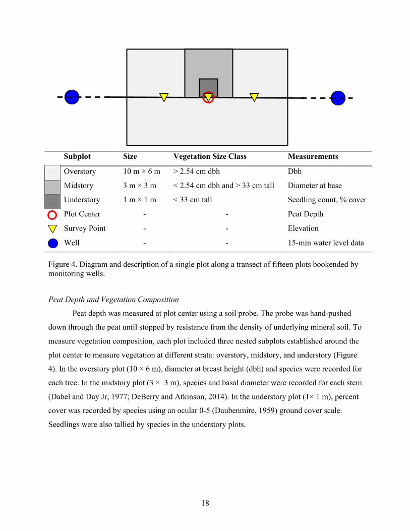
perpendicular to the corresponding ditch/road (Figure 3). We established fifteen plots along each

transect (Figure 4), spaced at 20 m intervals, to measure hydrologic regime, land surface

elevation, peat depths, and vegetation attributes (n = 75). Plots captured a wetness gradient both

within and across transects.

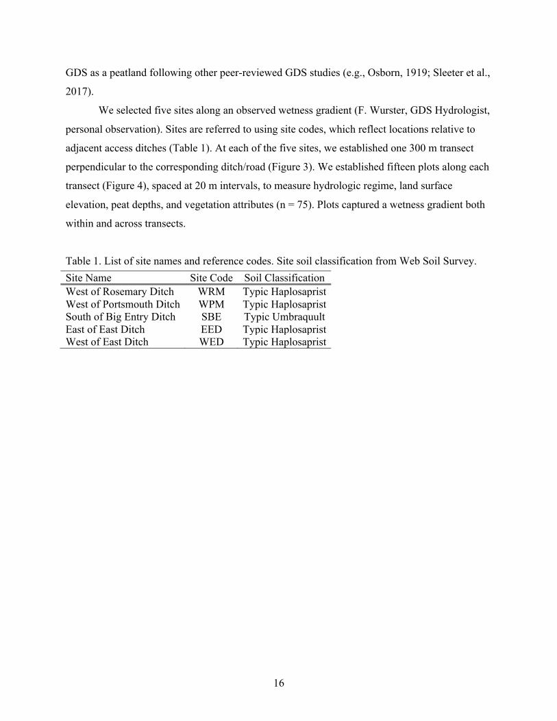
Table 1. List of site names and reference codes. Site soil classification from Web Soil Survey. Site Name Site Code Soil Classification West of Rosemary Ditch WRM Typic Haplosaprist West of Portsmouth Ditch WPM Typic Haplosaprist South of Big Entry Ditch SBE Typic Umbraquult East of East Ditch EED Typic Haplosaprist West of East Ditch WED Typic Haplosaprist

17

Figure 3. Transects (right pane, white lines) located in the northeastern corner of the Great Dismal Swamp with paired wells (blue circles) bookending each transect (courtesy of U.S. Fish and Wildlife Service).

2.3.2 Data Collection

Hydrologic Regime and Microtopography

To estimate hydrologic regime at each plot, we related continuous measures of water

level elevation to plot land surface elevation across each transect. Monitoring wells were

previously installed at each end of transects by GDS staff. Pressure transducers in each well

provided continuous 15-minute water level data for 16 months. Using an optical level and

leveling rod, we surveyed the relative elevation of plot center and plot center ± 3 meters to the

first well at each transect (Figure 4). A microtopography index at each plot was calculated as the

standard deviation of the three elevation points per plot. Using our surveyed elevations, we

interpolated between wells to estimate 15-minute water level height at each of the three surveyed

locations in each plot. This approach yielded spatial (3 locations per plot) and temporal water

level variation at each plot to explore relationships among hydrology, peat depth,

microtopography, and vegetation across all 75 plots.

WEDEED WPM

WRM

SBE

18

Subplot Size Vegetation Size Class Measurements

Overstory 10 m × 6 m > 2.54 cm dbh Dbh

Midstory 3 m × 3 m < 2.54 cm dbh and > 33 cm tall Diameter at base

Understory 1 m × 1 m < 33 cm tall Seedling count, % cover

Plot Center - - Peat Depth

Survey Point - - Elevation

Well - - 15-min water level data

Figure 4. Diagram and description of a single plot along a transect of fifteen plots bookended by monitoring wells.

Peat Depth and Vegetation Composition

Peat depth was measured at plot center using a soil probe. The probe was hand-pushed

down through the peat until stopped by resistance from the density of underlying mineral soil. To

measure vegetation composition, each plot included three nested subplots established around the

plot center to measure vegetation at different strata: overstory, midstory, and understory (Figure

4). In the overstory plot (10 × 6 m), diameter at breast height (dbh) and species were recorded for

each tree. In the midstory plot (3 × 3 m), species and basal diameter were recorded for each stem

(Dabel and Day Jr, 1977; DeBerry and Atkinson, 2014). In the understory plot (1× 1 m), percent

cover was recorded by species using an ocular 0-5 (Daubenmire, 1959) ground cover scale.

Seedlings were also tallied by species in the understory plots.

19

2.3.3 Data Analysis

We characterized hydrologic regime at both transect and plot level. Using three surveyed

locations at each plot, we calculated plot water level mean (i.e., mean over time and space), 10th

and 90th percentiles, and temporal standard deviation. Using plot-level water levels, we

calculated transect-scale water level mean (over time and space), 10th and 90th percentiles, and

temporal standard deviations. Microtopography at each plot was characterized by the index of

standard deviation of the three surveyed elevation points in each plot.

To characterize vegetation attributes in each plot, we calculated several metrics

separately for overstory, midstory, and seedling strata including species density, relative density

(sum of species density/sum of total density), frequency, richness, and diversity (Shannon-

Wiener Index). We also calculated overstory and midstory basal area for all species and relative

basal area (sum of species basal area/sum of total basal area) for maple. To better understand the

presence of maple, we calculated Importance Value (0-100%), which we calculated as the sum of

overstory relative maple basal area and relative maple density. We also calculated overstory

quadratic mean diameter (QMD) per transect, where ba is basal area (m2/ha) and tpha is trees per

hectare:

𝑄𝑀𝐷 =

𝑏𝑎𝑡𝑝ℎ𝑎

0.00007854

Understory cover scale numbers (0-5) by species were considered categorical variables. Mean

values for all metrics across plots characterized vegetation within each transect.

Presence/absence of understory obligate wetland species at each plot was also tallied by transect.

To evaluate relationships among hydrology, vegetation composition, and peat depth, we

performed three different analyses. First, we performed a transect-level categorical analysis in

JMP (SAS Institute Inc., 2012) using Analysis of Variance (α = 0.05) to compare vegetation

community attributes, peat depth, and microtopography across categorical wetness (via mean

water level height). When a significant difference was detected, we used Tukey’s honest

significant difference (HSD) post-hoc test to evaluate pair-wise differences between transects.

Second, we explored plot-level correlations (via Spearman’s correlation analysis) among

hydrologic regime metrics, vegetation attributes, microtopography, and peat depth across all 75

plots, with particular focus on correlations with maple importance. Lastly, we analyzed the suite

20

of vegetation and hydrologic parameters using nonmetric multidimensional scaling (NMDS) in R

(R Core Team, 2016), using ‘mds’ function in the ‘vegan’ package (Oksanen et al., 2017).

Vegetation parameters were input as processed data (e.g., whole strata density, basal area,

diversity, richness). Data were scaled to normalize values using the ‘scale’ function. To ensure

avoidance of local minima and maxima, the analysis was conducted using Euclidean distance

and seven random starts for 10,000 iterations. A stress test was used to determine goodness-of-

fit. A Shepard diagram was used to show the residual variability about the regression line and

determine the adequacy of the dimensional representation. Both vegetation vectors (i.e., data

input to create the NMDS ordination space) and hydrology vectors were fit to the axes using the

‘envfit’ function to show each parameter’s relationship with the spread of data in ordination

space.

2.4 Results We evaluated relationships among hydrologic regime, peat depth, microtopography, and

vegetation composition to better understand the hydrologic effects on GDS ecosystem structure

and function. We examined these relationships at different spatial scales using both transect-

(categorical) and plot- (continuous) level analyses.

2.4.1 Transect- and Plot-level Hydrology

We captured a gradient of hydrologic regime across transects. Transect mean water level

(i.e., average of plot-level temporal means) ranged from -0.58 m (at WRM) to 0.16 m above land

surface (at WED), varying significantly (P < 0.0001) between all transects, except SBE and EED

(Figure 5a). Temporal water level standard deviation at the transect-level (i.e., mean of plot-level

standard deviations) highlighted significant differences in water level variation across all

transects except EED and WED (Figure 5b). Similar trends across transects (driest to wettest

transect; WRM to WED) were also found for 10th (-0.97 to 0.01 m) and 90th percentiles (-0.33 to

0.24 m), revealing significant transect differences for both low and high water level conditions,

respectively (data not shown).

Our sampling design also captured a gradient of hydrologic regime at the plot level. Plot

mean water level ranged from -0.81 m to 0.40 m (see box-plot distributions in Figure 5a), and

standard deviation ranged from 0.35 m to 0.09 m (see Figure 5b). Water level 10th and 90th

21

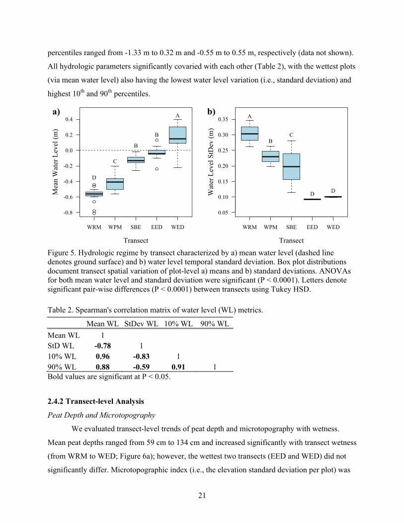
percentiles ranged from -1.33 m to 0.32 m and -0.55 m to 0.55 m, respectively (data not shown).

All hydrologic parameters significantly covaried with each other (Table 2), with the wettest plots

(via mean water level) also having the lowest water level variation (i.e., standard deviation) and

highest 10th and 90th percentiles.

Figure 5. Hydrologic regime by transect characterized by a) mean water level (dashed line denotes ground surface) and b) water level temporal standard deviation. Box plot distributions document transect spatial variation of plot-level a) means and b) standard deviations. ANOVAs for both mean water level and standard deviation were significant (P < 0.0001). Letters denote significant pair-wise differences (P < 0.0001) between transects using Tukey HSD. Table 2. Spearman's correlation matrix of water level (WL) metrics.

Mean WL StDev WL 10% WL 90% WL Mean WL 1

StD WL -0.78 1 10% WL 0.96 -0.83 1

90% WL 0.88 -0.59 0.91 1 Bold values are significant at P < 0.05.

2.4.2 Transect-level Analysis

Peat Depth and Microtopography

We evaluated transect-level trends of peat depth and microtopography with wetness.

Mean peat depths ranged from 59 cm to 134 cm and increased significantly with transect wetness

(from WRM to WED; Figure 6a); however, the wettest two transects (EED and WED) did not

significantly differ. Microtopographic index (i.e., the elevation standard deviation per plot) was

WRM WPM SBE EED WED

-0.8

-0.6

-0.4

-0.2

0.0

0.2

0.4

Transect

Mea

n W

ater

Lev

el (m

)

D

C

B

B

A

WRM WPM SBE EED WED

0.05

0.10

0.15

0.20

0.25

0.30

0.35

Transect

Wat

er L

evel

StD

ev (m

)

A

BC

D D

a) b)

22

generally lower at the drier transects and highest at the wettest two transects (EED and WED),

but not significantly (Figure 6b).

Figure 6. Transect means (± standard deviation) of plot-level a) peat depth and b) microtopography index along a gradient of increasing wetness (via transect mean water level). Microtopography index at each plot is defined as the standard deviation of three plot elevations. ANOVA for both peat depth and microtopography were significant (P < 0.05). Letters denote significant pair-wise differences (P < 0.05) between transects using Tukey HSD.

Vegetation Composition and Maple

For each stratum, we compared vegetation composition and structure across transects and

thus a wetness gradient. In the overstory stratum, tree size class distributions varied across

transects with higher frequencies of small diameter trees at wetter transects (Figure 7). Similarly,

QMD also decreased with wetness from 25 cm (at WRM) to 13 cm (at WED; Figure 7). Tree

density ranged from 750 to 2800 stems ha-1, and was significantly higher at the wettest two

transects (EED and WED; Figure 8a). However, maple relative tree density was highest at the

three driest transects (Figure 8b). Tree basal area showed no significant trend with wetness

(Figure 8c), whereas maple relative tree basal area was highest at the three driest transects

(Figure 8d). As a result, maple importance value (i.e., sum of maple relative tree basal area and

density) was significantly lower at the wettest transects (EED and WED; Figure 8e). Despite this

trend of maple importance, tree diversity (Shannon Index) showed no clear pattern with wetness

(Figure 8f). In the midstory stratum, shrub composition and structure also revealed no clear trend

with wetness. SBE had significantly higher shrub density and basal area than all other transects

(Figure 9a,b), but generally lower diversity (Figure 9c). Maple was not prevalent at the midstory

level. In the understory stratum, richness was generally higher at the wettest three transects, but

0

30

60

90

120

150

180

WRM WPM SBE EED WED

Peat

Dep

th (c

m)

Transect

a)

D

C B

A A

0

5

10

15

20

25

WRM WPM SBE EED WED

Mic

roto

pogr

aphy

In

dex

(cm

)

Transect

b)

C

ABC

BC

A AB

Wetness Wetness

23

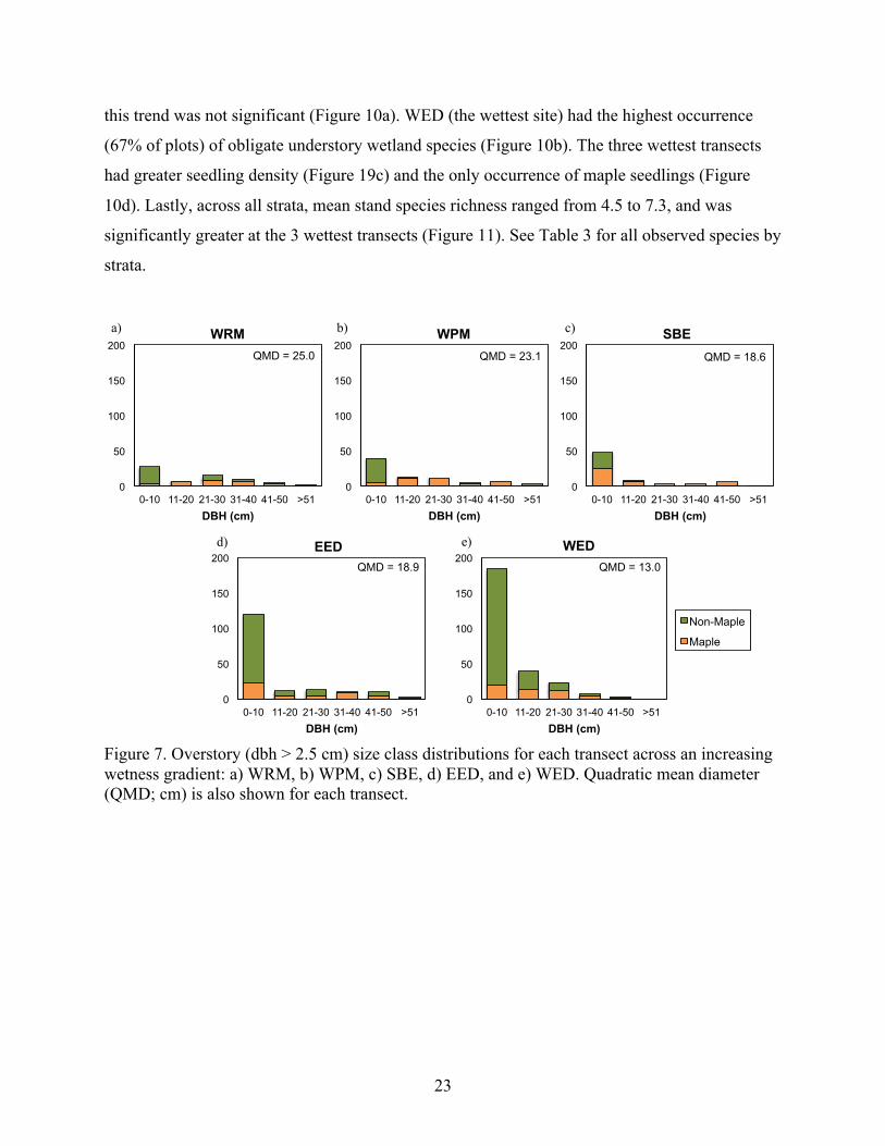
this trend was not significant (Figure 10a). WED (the wettest site) had the highest occurrence

(67% of plots) of obligate understory wetland species (Figure 10b). The three wettest transects

had greater seedling density (Figure 19c) and the only occurrence of maple seedlings (Figure

10d). Lastly, across all strata, mean stand species richness ranged from 4.5 to 7.3, and was

significantly greater at the 3 wettest transects (Figure 11). See Table 3 for all observed species by

strata.

Figure 7. Overstory (dbh > 2.5 cm) size class distributions for each transect across an increasing wetness gradient: a) WRM, b) WPM, c) SBE, d) EED, and e) WED. Quadratic mean diameter (QMD; cm) is also shown for each transect.

0

50

100

150

200

0-10 11-20 21-30 31-40 41-50 >51

DBH (cm)

WRM

0

50

100

150

200

0-10 11-20 21-30 31-40 41-50 >51

DBH (cm)

WPM

0

50

100

150

200

0-10 11-20 21-30 31-40 41-50 >51

DBH (cm)

SBE

0

50

100

150

200

0-10 11-20 21-30 31-40 41-50 >51

DBH (cm)

EED

0

50

100

150

200

0-10 11-20 21-30 31-40 41-50 >51

DBH (cm)

WED

Non-Maple

Maple

QMD = 23.1 QMD = 18.6

QMD = 18.9 QMD = 13.0

QMD = 25.0

a) b) c)

d) e)

24

Figure 8. Overstory analysis by transect mean (± standard deviation) of plot-level a) tree density, b) maple relative tree density, c) tree basal area, d) maple relative tree basal area, e) maple importance value, and f) tree diversity along a gradient of increasing wetness (via transect mean water level). Tukey HSD ordered letters are shown on plots if ANOVA was significant (P < 0.05).

0

1000

2000

3000

4000

Tree

Den

sity

(s

tem

s/ha

)

C C C

B

A a)

0

20

40

60

80

100

Tree

Bas

al A

rea

(m

2 /ha)

c)

0.0

0.3

0.6

0.9

1.2

Map

le R

elat

ive

Den

sity

(-) ABC A AB

BC

C

b)

0.0

0.4

0.8

1.2

1.6

Map

le R

elat

ive

B

asal

Are

a (-

) ABC A AB

BC C

d)

0.0

0.4

0.8

1.2

1.6

WRM WPM SBE EED WED

Tree

Div

ersi

ty (-

)

Transect

BC A ABC AB

C

f)

0

20

40

60

80

100

WRM WPM SBE EED WED

Map

le Im

porta

nce

Va

lue

(%)

Transect

AB A A

B B

e)

Wetness Wetness

25

Figure 9. Shrub analysis by transect mean (± standard deviation) of plot-level a) shrub density, b) shrub basal area, and c) shrub diversity along a gradient of increasing wetness (via transect mean water level). Tukey HSD ordered letters are shown on plots if ANOVA was significant (P < 0.05).

0

100

200

300

400

500

WRM WPM SBE EED WED

Shru

b D

ensi

ty

(thou

sand

stem

s/ha

)

B B B B

A a)

-0.4

0.0

0.4

0.8

1.2

1.6

WRM WPM SBE EED WED

Shru

b D

iver

sity

(-)

Transect

c) A

C

AB

BC

ABC

0

4

8

12

16

20

WRM WPM SBE EED WED

Shr

ub B

asal

Are

a

(m2 /h

a)

b)

AB B

B

A

AB

Wetness

26

Figure 10. Understory analysis by transect mean (± standard deviation) of plot-level a) richness, b) count of plots with presence of obligate wetland (OBL) species, c) seedling density, and d) seedling maple relative density along a gradient of increasing wetness (via transect mean water level). Tukey HSD ordered letters are shown on plots if ANOVA was significant (P < 0.05).

Figure 11. Transect mean (± standard deviation) of plot-level species richness across all strata along a gradient of increasing wetness (via transect mean water level). Letters denote significant differences (P < 0.0001) between transects using Tukey HSD.

0

1

2

3

4

5

6 R

ichn

ess (

-)

a)

0

2

4

6

8

10

12

Und

erst

ory

OB

L Sp

ecie

s Pr

esen

ce (#

of p

lots

)

b)

0

5

10

15

20

25

30

WRM WPM SBE EED WED

See

dlin

g D

ensi

ty

(ste

ms/

m2 )

Transect

c)

0.0

0.4

0.8

1.2

WRM WPM SBE EED WED

See

dlin

g M

aple

R

elat

ive

Den

sity

(-)

Transect

d) A

C C

AB

BC

Wetness Wetness

0

2

4

6

8

10

12

WRM WPM SBE EED WED

Stan

d R

ichn

ess (

-)

Transect

B B

A A A

Wetness

27

Table 3. List of observed species. Species are included in the stratum where it appeared most, with 4-letter code used in this study and the Atlantic and Gulf Coastal Plain (AGCP) Regional Wetland Plant List Classification: upland (UPL), facultative upland (FACU), facultative (FAC), facultative wetland (FACW), and obligate wetland (OBL). Common Name Scientific Name Code AGCP Tree Loblolly pine Pinus taeda L. PITA FAC Pond pine Pinus serotina Michx. PISE FACW Bald cypress Taxodium distichum L. TADI OBL Pond cypress Taxodium ascendens Brongn. TAAS OBL Tulip-poplar Liriodendron tulipifera L. LITU FACU Sweetbay Magnolia virginiana L. MAVI FACW Redbay Persea borbonia L. PEBO FACW Pawpaw Asimina triloba L. ASTR FAC Sweetgum Liquidambar styraciflua L. LIST FAC American holly Ilex opaca Ait. ILOP FAC Red maple Acer rubrum L. ACRU FAC Blackgum Nyssa sylvatica Marsh. NYSY FAC Swamp Tupelo Nyssa biflora Walt. NYBI OBL Black Oak Quercus velutina Lam. QUVE UPL Shrub Sweet pepperbush Clethra alnifolia L. CLAL FACW Giant cane Arundinaria gigantea Walt. ARGI FACW Highbush blueberry Vaccinium corymbosum L. VACO FACW Herb Virginia creeper Parthenocissus quinquefolia L. PAQU FACU Netted chain fern Woodwardia areolata L. WOAR OBL Muscadine grape Vitis rotundifolia Michx. VIRO FAC Bladderwort Utricularia spp UTRI OBL Poison Ivy Toxicodendron radicans L. TORA FAC Greenbriar Smilax spp SMSP FAC Sphagnum moss Sphagnum spp SPHA OBL Wild strawberry Fragaria vesca L. FRVE UPL Virginia chain fern Woodwardia virginica L. WOVI OBL

28

2.4.3 Plot-level Analysis

Peat Depth and Microtopography

We evaluated relationships of peat depth and microtopography with hydrologic metrics at

the plot level. Peat depth had a strong positive relationship with mean water level (Figure 12a)

and a strong negative relationship with water level standard deviation (Figure 12b).

Microtopographic index had a weak but positive relationship with mean water level (Figure 12c)

and a negative (but stronger) relationship with water level standard deviation (Figure 12d). Peat

depth and microtopographic index covaried significantly (Spearman’s ρ = 0.36; data not shown).

Figure 12. Plot-level analysis of a-b) peat depth and c-d) microtopography vs. hydrologic metrics (mean water level and standard deviation). All relationships were significant via Spearman’s correlation (P < 0.05).

Vegetation Composition and Maple

At the plot level, we evaluated correlations among hydrologic and vegetation metrics

across strata, with a focus on maple importance. At the overstory stratum, plot tree density

significantly increased with mean water level (Figure 13a), and had a strong significant

correlation with all other hydrology metrics (Table 4). In contrast, tree basal area and tree

0

5

10

15

20

25

30

35

-1.0 -0.5 0.0 0.5 Mic

roto

pogr

aphy

Inde

x (c

m)

Mean Water Level (m)

ρ = 0.36

0

40

80

120

160

200

Peat

Dep

th (c

m)

ρ = 0.78 a)

c)

ρ = -0.81 b)

0.0 0.1 0.2 0.3 0.4 Water Level Standard Deviation (m)

ρ = -0.46 d)

29

diversity showed no significant relationships with hydrologic metrics (Table 4). Maple relative

tree density, relative basal area, and importance value (Figure 13b) were all negatively correlated

with mean water level and positively correlated with water level standard deviation (Table 5).

However, absolute maple tree density and basal area had no significant correlation with

hydrologic metrics (Table 5). At the midstory stratum, plot shrub density and shrub basal area

showed no significant relationships with hydrologic metrics (Table 4). However, shrub diversity

was positively correlated with mean water level and negatively correlated with water level

standard deviation (Table 4). While understory richness showed no significant relationships with

hydrology (Table 4), seedling diversity and density were significantly correlated with some

hydrologic metrics, including negative correlations with water level standard deviation (Table 4).

Maple seedling density and relative density were positively correlated with mean water level and

negatively correlated with water level standard deviation (Table 5).

Overall stand richness (across all strata) increased significantly with mean water level (P

= 0.0001; Figure 13c, Table 4). Stand richness was also positively correlated with 10th percentile

and 90th percentile water level, negatively correlated with water level standard deviation, and had

no significant correlation with microtopography (Table 4, Figure 13d). Lastly, stand richness had

a significant (ρ = -0.36) negative relationship with maple importance; however, maple

importance did not significantly covary with any other non-maple vegetation parameters (Table

6).

30

Figure 13. Plot-level analysis of vegetation parameters: a) tree density vs. mean water level, b) maple importance value vs. mean water level, c) stand richness vs. mean water level, d) stand richness vs. microtopography index. Bold values denote Spearman’s correlation significance (P < 0.05).

0

1000

2000

3000

4000

5000

-1.0 -0.5 0.0 0.5

Tree

Den

sity

(ste

ms/

ha)

Mean Water Level (m)

ρ= 0.62 a)

0

2

4

6

8

10

12

-1.0 -0.5 0.0 0.5

Stan

d R

ichn

ess (

-)

Mean Water Level (m)

ρ= 0.43 c)

0

2

4

6

8

10

12

0 10 20 30 40

Stan

d R

ichn

ess (

-)

Microtopography Index (cm)

d) ρ= 0.23

0

20

40

60

80

100

-1.0 -0.5 0.0 0.5

Map

le Im

porta

nce

Valu

e (%

)

Mean Water Level (m)

b) ρ= -0.34

31

Table 4. Spearman’s correlation matrix of vegetation vs. hydrologic metrics.

Mean WL StDev WL 10% WL 90% WL Microtopo Stand Richness 0.43 -0.46 0.42 0.30 0.23 Tree Diversity -0.19 0.03 -0.16 -0.05 0.07 Tree Density 0.62 -0.51 0.58 0.50 0.31 Tree Basal Area 0.00 -0.12 0.05 0.00 0.11 Shrub Diversity 0.28 -0.40 0.27 0.21 0.15 Shrub Density 0.12 -0.09 0.07 0.00 0.04 Shrub Basal Area -0.02 0.07 -0.06 -0.10 -0.10 Understory Richness 0.02 -0.14 -0.05 -0.20 0.10 Seedling Diversity 0.21 -0.31 0.20 0.11 0.24 Seedling Density 0.33 -0.41 0.28 0.10 0.16 Bold values are significant at P < 0.05. Table 5. Spearman’s correlation matrix of maple vs. hydrologic metrics.

Mean WL StDev WL 10% WL 90% WL Microtopo Maple Importance Value -0.34 0.30 -0.31 -0.23 -0.14 Tree Maple Density 0.09 -0.06 0.11 0.14 0.04 Tree Maple Relative Density -0.38 0.32 -0.34 -0.26 -0.13 Tree Maple BA -0.19 0.06 -0.12 -0.15 -0.06 Tree Maple Relative BA -0.32 0.30 -0.30 -0.23 -0.16 Seedling Maple Density 0.35 -0.41 0.31 0.17 0.09 Seedling Maple Relative Density 0.33 -0.39 0.31 0.19 0.08 Bold values are significant at P < 0.05.

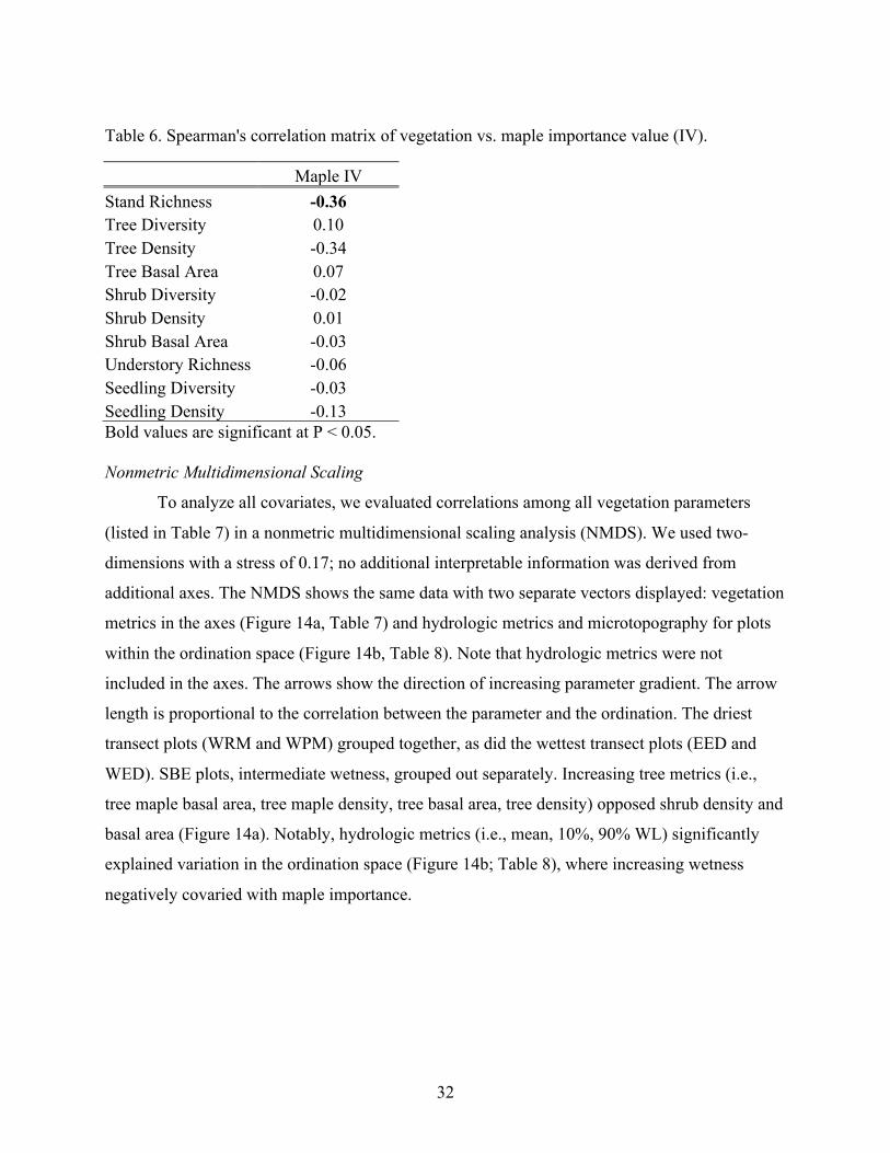
32

Table 6. Spearman's correlation matrix of vegetation vs. maple importance value (IV).

Maple IV Stand Richness -0.36 Tree Diversity 0.10 Tree Density -0.34 Tree Basal Area 0.07 Shrub Diversity -0.02 Shrub Density 0.01 Shrub Basal Area -0.03 Understory Richness -0.06 Seedling Diversity -0.03 Seedling Density -0.13 Bold values are significant at P < 0.05. Nonmetric Multidimensional Scaling

To analyze all covariates, we evaluated correlations among all vegetation parameters

(listed in Table 7) in a nonmetric multidimensional scaling analysis (NMDS). We used two-

dimensions with a stress of 0.17; no additional interpretable information was derived from

additional axes. The NMDS shows the same data with two separate vectors displayed: vegetation

metrics in the axes (Figure 14a, Table 7) and hydrologic metrics and microtopography for plots

within the ordination space (Figure 14b, Table 8). Note that hydrologic metrics were not

included in the axes. The arrows show the direction of increasing parameter gradient. The arrow

length is proportional to the correlation between the parameter and the ordination. The driest

transect plots (WRM and WPM) grouped together, as did the wettest transect plots (EED and

WED). SBE plots, intermediate wetness, grouped out separately. Increasing tree metrics (i.e.,

tree maple basal area, tree maple density, tree basal area, tree density) opposed shrub density and

basal area (Figure 14a). Notably, hydrologic metrics (i.e., mean, 10%, 90% WL) significantly

explained variation in the ordination space (Figure 14b; Table 8), where increasing wetness

negatively covaried with maple importance.

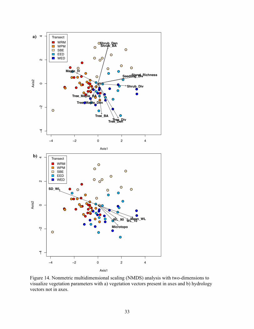
33

Figure 14. Nonmetric multidimensional scaling (NMDS) analysis with two-dimensions to visualize vegetation parameters with a) vegetation vectors present in axes and b) hydrology vectors not in axes.

●

●●

●●

●●

● ●

●

●

●

●

●

●

●

●

●●

●

●

●

●

●

●

●

●

●

●

●

●

●

●

●

●

●

●

●

●

●

●

●

●

●

●

●

●

●

●

●

● ●

●

●

●

●

●

●● ●

●

●

● ●●

●

●

●

●●

●

●

●

−4 −2 0 2 4

−4−2

02

4

Axis1

Axis2

TransectWRMWPMSBEEEDWED

Stand_Richness

Tree_Div

Tree_Maple_BA

Tree_Maple_Den

Tree_BATree_Den

Maple_IV

Shrub_Div

Shrub_BAShrub_Den

Seedling_Div

a)

●

●●

●●

●●

● ●

●

●

●

●

●

●

●

●

●●

●

●

●

●

●

●

●

●

●

●

●

●

●

●

●

●

●

●

●

●

●

●

●

●

●

●

●

●

●

●

●

● ●

●

●

●

●

●

●● ●

●

●

● ●●

●

●

●

●●

●

●

●

−4 −2 0 2 4

−4−2

02

4

Axis1

Axis2

TransectWRMWPMSBEEEDWED

b)

Mean_WL

SD_WL

WL_10WL_90

Microtopo

b)

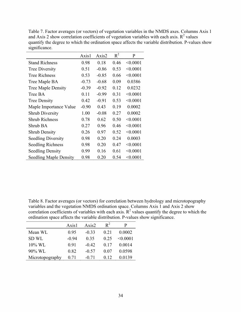
34

Table 7. Factor averages (or vectors) of vegetation variables in the NMDS axes. Columns Axis 1 and Axis 2 show correlation coefficients of vegetation variables with each axis. R2 values quantify the degree to which the ordination space affects the variable distribution. P-values show significance.

Axis1 Axis2 R2 P Stand Richness 0.98 0.18 0.46 <0.0001 Tree Diversity 0.51 -0.86 0.53 <0.0001 Tree Richness 0.53 -0.85 0.66 <0.0001 Tree Maple BA -0.73 -0.68 0.09 0.0386 Tree Maple Density -0.39 -0.92 0.12 0.0232 Tree BA 0.11 -0.99 0.31 <0.0001 Tree Density 0.42 -0.91 0.53 <0.0001 Maple Importance Value -0.90 0.43 0.19 0.0002 Shrub Diversity 1.00 -0.08 0.27 0.0002 Shrub Richness 0.78 0.62 0.50 <0.0001 Shrub BA 0.27 0.96 0.46 <0.0001 Shrub Density 0.26 0.97 0.52 <0.0001 Seedling Diversity 0.98 0.20 0.24 0.0003 Seedling Richness 0.98 0.20 0.47 <0.0001 Seedling Density 0.99 0.16 0.61 <0.0001 Seedling Maple Density 0.98 0.20 0.54 <0.0001 Table 8. Factor averages (or vectors) for correlation between hydrology and microtopography variables and the vegetation NMDS ordination space. Columns Axis 1 and Axis 2 show correlation coefficients of variables with each axis. R2 values quantify the degree to which the ordination space affects the variable distribution. P-values show significance.

Axis1 Axis2 R2 P Mean WL 0.95 -0.33 0.21 0.0002 SD WL -0.94 0.35 0.25 <0.0001 10% WL 0.91 -0.42 0.17 0.0014 90% WL 0.82 -0.57 0.07 0.0598 Microtopography 0.71 -0.71 0.12 0.0139

35

2.5 Discussion In this work, we sought to explore hydrologic controls on peat depth, microtopography,

and vegetation composition, testing two specific hypotheses:

H1) Increased wetness (e.g., shallower water table) increases peat depth and microtopographic variation. H2) Increased wetness decreases maple importance and increases overall diversity.

To do so, we coupled in situ hydrologic monitoring with surveys of peat depths, surface

elevation, and vegetation along a gradient of wetness. Our findings highlight hydrologic

variation at plot and transect scales and how such variation influences peat depth,

microtopography, and vegetation composition. As such, research findings will inform hydrologic

restoration at GDS and, more broadly, advance our understanding of interactions between

hydrology and ecosystem structure and function in temperate peatlands.

Hydrology

Our hydrologic monitoring approach allowed estimates of continuous water level across

75 plots, capturing variation in hydrologic regime among and within transects. Differences in

water level dynamics across transects demonstrate marked spatial variation in our focus area of

GDS (i.e., NE corner; Figure 3), and likely effects of ditches and roads to induce such variation

across landscape sections. Transects ranged from wet with stable water levels (e.g., mean water

level ± standard deviation at WED = 0.16 ± 0.1 m) to relatively dry with more variable water

levels (e.g., WRM = -0.58 ± 0.3 m; Figure 5). Differences in plot water levels highlight variation

within transects, pointing to local controls (e.g., elevation, distance to ditch) and likely increasing

local habitat complexity. Plot mean water level and standard deviation data captured end

members of deep (-0.81 ± 0.35 m) and shallow water table conditions (0.40 ± 0.09 m), where

wetter plots also had more stable water levels (Figure 5b; Table 2). Of the 75 plots monitored, 39

were never flooded, 25 were intermittently flooded, and 11 were perennially flooded; as such,

plots captured a gradient of hydroperiod conditions.

The range of hydrologic regimes we measured spanned typical values of dominant

swamp community types (e.g., cedar to cypress) found at GDS. At the driest end, pocosins (in

New Jersey) typically have mean water levels between -0.35 and -0.55 m, with variable water

level fluctuation (standard deviation of 0.28 m; Zampella et al., 2001; Yu and Ehrenfeld, 2010).

36

Similarly, more shallow and variable water tables (ca. -0.20 to -0.25 m ± 0.22 m) also typify

New Jersey maple swamps (Zampella et al., 2001; Yu and Ehrenfeld, 2010). Cedar swamp water

levels are generally more stable and shallower (-0.10 to 0.03 m above land surface; Little, 1950;

Yu and Ehrenfeld, 2010), and typically do not fall below -0.15 m (Parrott et al., 1981; Atkinson

et al., 2003). At the wettest end, cypress-tupelo swamp mean water level occurs between 0.1 to -

0.5 m, ranging from 0.9 to -1.0 m (Aust and Lea, 1992; Crownover et al., 1995; Keeland et al.,

1997).

Despite capturing a hydrologic gradient between transects, our sampling design did

somewhat limit our ability to infer hydrologic variation and controls on ecosystem properties

across GDS. For example, our transects were solely in the northeastern corner of GDS,

potentially missing other forest communities, as well as wetter, drier, and more hydrologically

variable locations. Moreover, we only had two wells per transect and relied on land surface

elevations and interpolation to estimate water levels at each plot. However, high saturated

conductivity in the upper peat, and thus especially at high water levels (Lichtler and Walker,

1974), likely minimized local deviation from a broader hydraulic gradient over the 300 m

transects. Lastly, hydrologic data were only collected for 16 months. However, relative

differences in hydrologic regime among plots over this monitoring period likely hold across

longer periods and varying climate, provided there are no changes to ditch control. Despite these

limitations, our monitored sites exhibit clear and significant differences in hydrologic regime to

evaluate relative controls on peat depth, microtopography, and vegetation.

Peat and Microtopography

We found clear hydrologic controls on peat depth confirming our hypothesis of increased

peat depth with increased wetness. Constant soil saturation is an important regulator of organic

matter decomposition and thus peat accretion and carbon storage (Reddy and Patrick, 1975). As

expected, peat depth increased significantly with mean water level at both the transect-level

(Figure 6a) and plot-level (Figure 12a). Peat depth also increased with decreasing water level

standard deviation (Figure 12b). However, there was a strong (negative) covariance between

mean water level and standard deviation; that is, we did not capture sites with both high mean

water level and high standard deviation water level, limiting our ability to separate controls of

mean and variation in water levels. Plot peat depth ranged from 40 cm to 160 cm (Figure 12a),

37

with a mean of 1 m across all plots. These depths are similar but somewhat smaller compared to

peat depths in temperate cedar swamps with similar hydrologic regimes (i.e., water levels

ranging from -20 to 30 cm above land surface; Golet and Lowry, 1987). For example, Ott and

Chimner (2016) measured peat depths from 40 cm to 325 cm, with an average of 112 cm in

cedar peatlands in northern Minnesota and Michigan. Yu and Ehrenfeld (2010) found peat depths

up to 200 cm in New Jersey cedar swamps. Note that our peat depth observations were

constrained to one region of GDS, and previous work has documented depths exceeding 3 m in

other GDS locations (Oaks and Coch, 1973). To our knowledge, however, our work is the first in

GDS to link peat depths with hydrologic regime, thereby highlighting hydrologic controls on the

carbon storage function valued in GDS.

We also found differences in microtopography across both transects and plots, with a

moderate but significant relationship with hydrologic regime. We defined our microtopographic

index as the local standard deviation in elevations at three surveyed points per plot. The highest

microtopographic variation was found at the wettest two sites, where plot elevation standard

deviations ranged from 3 cm to 30 cm, possibly due to windthrow. Concordantly,

microtopographic index had a significant positive correlation with mean water level (Figure 12c)

and negative correlation with water level standard deviation (Figure 12d), highlighting the

influence of sustained, wet conditions to support hummock and hollow formation. Formation

mechanisms for peatland microtopography vary but all require saturated soils. Ehrenfeld (1995b)

identified windthrow as the main mechanism for hummock formation (up to 70-100 cm in

height) in cedar swamps, where shallow rooted trees (due to high water level) in peat soils are

vulnerable to wind disturbance. Spatially varying organic matter accumulation through

concentrated litter fall or root turnover on more productive (less anaerobic) hummocks can

further feedback to hummock development (Ehrenfeld, 1995a; Bruland and Richardson, 2005).

Sediment deposition is another mechanism for microtopography (Bruland and Richardson,

2005), but minimal sediment-rich surface flow within GDS (Lichtler and Walker, 1974) makes

those inputs an unlikely formative process. Regardless of formation processes, our findings point

to hydrologic controls on microtopography and its feedback to spatial heterogeneity in

hydrologic regime and associated habitat.

Microtopographic variation, and thus spatial variation in hydrology, is known to

influence species richness in wetlands. Studies have observed increased herbaceous richness with

38

increased microtopographic heterogeneity, with different species showing a preference for either

high or low elevation locations (Vivian-Smith, 1997; Bruland and Richardson, 2005). Although,

Ehrenfeld (1995a) found that wetland woody plant species, especially tree seedlings, prefer only

high elevation sites. In our work, microtopographic index had a positive significant correlation

with tree density and seedling diversity (Table 4), highlighting possible roles of local elevation

variation on vegetation composition. Overall, stand richness was also positively correlated with

microtopographic index, though not significantly. Due to covariance in mean water level,

microtopography, and vegetation composition, more plots in locations with diverse hydrologic

regimes may be necessary to completely isolate and test the relationships between

microtopography and vegetation composition.

Vegetation Composition and Maple Importance

Hydrologic regime can exert strong controls on wetland vegetation by influencing

productivity (e.g., stand basal areas), tree regeneration, and species composition. More

specifically, wetter sites can exclude more facultative species (e.g., mixed hardwoods; Burke et

al., 2003) but also reduce productivity of remaining obligate species through anaerobic stress

(Vann and Megonigal, 2002); both the degree of species selection and influence of anaerobic

stress vary across species and hydrologic conditions (Angelov et al., 1996). At both transect and

plot levels, we observed hydrologic influences on vegetation composition and structure, although

the significance and direction of this influence varied across strata and vegetation metric. While

we did not directly measure stand productivity, our measurements of shrub and tree densities and

basal areas provide some inferences. There was no correlation between hydrologic regime and

basal areas; however, both transect and plot-level analyses demonstrated strong positive

associations between wetness and tree density (Figure 7, 8a, 13a; Table 4). No increase in tree

basal area along with increase in tree density suggests smaller trees at wetter sites, as

demonstrated with transect size class distributions (Figure 7). This is possibly a result of reduced

productivity of individual trees due to water stress (e.g., Vann and Megonigal, 2002) and/or

stand history and age. There were no evident associations between shrub structure and

hydrologic regime, but clearly a site-level effect (e.g., SBE; Figure 9, Table 4). In contrast,

seedling density (and for maple, a facultative species) increased significantly with mean water

level (Figures 10c-d; Table 4, 5), which is in agreement with measured tree density but not with

39

often observed lower regeneration under wetter conditions (Malecki et al., 1983; Ehrenfeld,

1995a). We could not explicitly test hydrologic influences on stand level diversity (H2) due to

varying nested plot sizes, but diversity at each stratum failed to confirm our general prediction.

However, stand-level richness did increase with wetness, at both transect (Figure 11) and plot

levels (although weakly; Figure 13d, Table 4), which both points to hydrologic and additional

(e.g., seed source, selective logging) controls on species selection and composition.

Our hypothesis of increased species diversity with wetness (H2) was founded on

predictions that wetness decreases maple importance, thereby increasing community diversity.

At both transect and plot levels, we found decreases in maple relative basal area, relative tree

density, and importance value with increased wetness, comporting with our prediction. However,

correlation between maple importance and stand richness was only weakly negative (but

significant; Table 6), and no significant associations were found between other stand-level

vegetation characteristics and maple, suggesting other influences on composition, such as

selective logging. Also, we found no significant relationship between absolute maple tree density

or basal area with wetness (Table 5). But, we did find significantly decreased relative maple tree

density and basal area at wetter sites, meaning there were more non-maple trees at wetter sites.

More non-maple trees at wetter sites is consistent with increased tree densities and the inference

of more but smaller trees at wetter sites.

To synthesize our suite of measured variables (e.g., composition and structure across

strata, hydrologic regimes), we conducted NMDS ordination analysis. To do so, we only used

vegetation parameters as axes inputs to explore how plots were grouped by vegetation

characteristics, and then to quantify the degree to which hydrologic parameters explained

vegetation variation among plots. When delineated by transect (colored plots in Figure 14),

grouping of plots within their own transect was clear, highlighting within and in some cases

between (WRM and WPM, EED and WED) transect similarities. Hydrologic parameters

significantly correlated with the ordination space (Figure 14b, Table 8), further demonstrating

the hydrologic control on vegetation composition in GDS. For example, the maple importance

vector falls opposite the mean water level vector, indicating a negative relationship between the

two.

Our work points to possible stress to maple trees (but not seedlings) under wetter

conditions, with associated increases in stand richness. Higher water levels could reduce maple

40

canopies (i.e., leaf area but not tree density), allowing more non-maple trees to compete for light

and increasing tree density and stand richness across strata (Malecki et al., 1983; Vann and

Megonigal, 2002). In contrast to our overstory maple measurements, we found increased relative

density of maple seedlings with wetness (Figure 10d, Table 5), suggesting a potential for

continued maple presence (via regeneration from similar absolute maple tree densities) across

hydrologic regimes (Malecki et al., 1983).

Previous work at GDS has called for hydrologic restoration (via more controlled and reduced

drainage) to restore vegetation composition back to a more historical state and sequester carbon

in the form of peat accretions. For example, Atkinson (2003) concluded that without hydrologic

restoration, it is likely that previous cedar-dominated sites will continue to yield to species other

species, including maple. Our findings add to this work by providing quantified relationships to

target locations and specific hydrologic regimes to meet restoration goals. Future work should

conduct measurements of leaf area index (LAI) to explore possible reduction in canopy cover

(especially maple), and associated effects to tree and seedling densities, with increased wetness.

Moreover, work is needed to understand ongoing stand succession under contemporary

hydrologic regimes, paying attention to shade tolerance (especially maple regeneration) and

possible canopy stress. This could include exploring if maple can sustain as a climax community,

and if so, exploring the possibility that hydrologic regimes can be altered to make maple less

competitive.

Conclusions

In this work, we sought to elucidate hydrologic controls on vegetation composition and

peat depths, and ultimately to inform ongoing restoration efforts at GDS. Findings support our

predictions in that at sites of increased wetness, we found thicker peat, more microtopographic

variation, lower maple importance, and higher stand richness. However, more research is needed,

especially to examine how maple importance affects community composition in other locations

across GDS. Moreover, while the hydrologic control on peat depths is clear, more work is

needed to understand the complex interactions between hydrologic regime and vegetation

organic matter inputs that together determine peat accretion rates. Going forward, new

restoration efforts at GDS should be coupled with continued research and monitoring to

adaptively achieve restoration goals. From our findings, we conclude that the hydrologic

41

influences to maple importance and peat thickness (and resulting carbon storage) at GDS support

the use of hydrology as a major management tool.

Literature Cited Anderson, J. A. R. 1983. The Tropical Peat Swamps of Western Malesia. Mires: Swamp, Bog,

Fen and Moor: Regional Studies. Angelov, M. N., S. S. Sung, W. R. Harms, P. P. Kormanik, and C. C. Black. 1996. Long-and

Short-Term Flooding Effects on Survival and Sink-Source Relationship of Swamps-Adapted Tree Species. Tree Physiology 16, 5: 477–484.

Atkinson, R. B., J. W. DeBerry, D. T. Loomis, E. R. Crawford, R. T. Belcher, R. B. Atkinson, R. T. Belcher, D. A. Brown, and J. E. Perry. 2003. Water Tables in Atlantic White Cedar Swamps: Implications for Restoration. In Atlantic White Cedar Restoration Ecology and Management, Proceedings of a Symposium. Christopher Newport University, Newport News, 137–150.

Aust, W. M., and R. Lea. 1992. Comparative Effects of Aerial and Ground Logging on Soil Properties in a Tupelo-Cypress Wetland. Forest Ecology and Management 50, 1–2: 57–73.

Bruenig, E. F. 1990. Oligotrophic Forested Wetlands in Borneo. Ecosystems of the World 15: 299–334.

Bruland, G. L., and C. J. Richardson. 2005. Hydrologic, Edaphic, and Vegetative Responses to Microtopographic Reestablishment in a Restored Wetland. Restoration Ecology 13, 3: 515–523

Burke, M. K., S. L. King, D. Gartner, and M. H. Eisenbies. 2003. Vegetation, Soil, and Flooding Relationships in a Blackwater Floodplain Forest. Wetlands 23, 4: 988–1002.

Carter, V., P. T. Gammon, and M. K. Garrett. 1994. Ecotone Dynamics and Boundary Determination in the Great Dismal Swamp. Ecological Applications, 189–203.

Casanova, M. T., and M. A. Brock. 2000. How Do Depth, Duration and Frequency of Flooding Influence the Establishment of Wetland Plant Communities? Plant Ecology 147, 2: 237–250.

Crownover, S. H., N. B. Comerford, D. G. Neary, and J. Montgomery. 1995. Horizontal Groundwater Flow Patterns through a Cypress Swamp-Pine Flatwoods Landscape. Soil Science Society of America Journal 59, 4: 1199–1205.

Dabel, C. V., and F. P. Day Jr. 1977. Structural Comparisons of Four Plant Communities in the Great Dismal Swamp, Virginia. Bulletin of the Torrey Botanical Club, 352–360.

Day Jr, F. P. 1985. Tree Growth Rates in the Periodically Flooded Great Dismal Swamp. Castanea, 1985, 89–95.

Daubenmire, R. 1959. A Canopy-Coverage Method of Vegetational Analysis. Northwest Science 33, 1: 43–64.

42

DeBerry, J. W., and R. B. Atkinson. 2014. Aboveground Forest Biomass and Litter Production Patterns in Atlantic White Cedar Swamps of Differing Hydroperiods. Southeastern Naturalist 13, 4: 673–690.

Ehrenfeld, J. G. 1995. Microsite Differences in Surface Substrate Characteristics in Chamaecyparis Swamps of the New Jersey Pinelands. Wetlands 15, 2: 183–189.

Ehrenfeld, J. G. 1995. Microtopography and Vegetation in Atlantic White Cedar Swamps: The Effects of Natural Disturbances. Canadian Journal of Botany 73, 3: 474–484.

Francis, H. E. 1959. Soil Survey for Norfolk County, Virginia, 53.

Golet, F.C., A.J.K. Calhoun, W.R. DeRagon, D.J. Lowry, and A.J. Gold. 1993. Ecology of Red Maple Swamps in the Glaciated Northeast: A Community Profile. Washington, D.C.

Hugron, S., J. Bussières, and L. Rochefort. 2013. Tree Plantations within the Context of Ecological Restoration of Peatlands: Practical Guide. Peatland Ecology Research Group, Université Laval, Québec, Québec, Canada.

Keeland, B. D., W. H. Conner, and R. R. Sharitz. 1997. A Comparison of Wetland Tree Growth Response to Hydrologic Regime in Louisiana and South Carolina. Forest Ecology and Management 90, 2: 237–250.

Kuhry, P., B. J. Nicholson, L. D. Gignac, D. H. Vitt, and S. E. Bayley. 1993. Development of Sphagnum-Dominated Peatlands in Boreal Continental Canada. Canadian Journal of Botany 71, 1: 10–22.

Legrand Jr, H. E. 2000. The Natural Features of Dismal Swamp State Natural Area, North Carolina. The Natural History of the Great Dismal Swamp, Omni, Madison, Wisconsin, 41–50.

Levy, G. F. 1991. The Vegetation of the Great Dismal Swamp: A Review and an Overview. Virginia Journal of Science 42, 4: 411–418.

Levy, G. F., and S. W. Walker. 1979. Forest Dynamics in the Dismal Swamp of Virginia. The Great Dismal Swamp. Old Dominion University Research Foundation, Inc.

Lewis, I. F., and E. C. Cocke. 1929. Pollen Analysis of Dismal Swamp Peat. Elisha Mitchell Scientific Society.

Lichtler, W., F., and P. Walker. 1974. Hydrology of the Dismal Swamp, Virginia-North Carolina. Geological Survey - Water Resources Division, no. 74–39.

Lilly, J. P. 1981. A History of Swamp Land Development in North Carolina. Malecki, R. A., J. R. Lassoie, E. Rieger, and T. Seamans. 1983. Effects of Long-Term Artificial

Flooding on a Northern Bottomland Hardwood Forest Community. Forest Science 29, 3: 535–544.

Oaks, R. Q., and N. K. Coch. 1973. Post-Miocene Stratigraphy and Morphology, Southeastern Virginia. Commonwealth of Virginia, Division of Mineral Resources.

Oksanen, J, F. G. Blanchet, M. Friendly, R. Kindt, P. Legendre, D. McGlinn, P. Minchin, et al. 2017. Vegan: Community Ecology Package (version 2.4-2).

43

Osborn, C. C. 1919. Peat in the Dismal Swamp, Virginia and North Carolina. Contribution to Economic Geology Bull 711, 4.

Ott, C. A., and R. A. Chimner. 2016. Long-Term Peat Accumulation in Temperate Forested Peatlands (Thuja Occidentalis Swamps) in the Great Lakes Region of North America. MIRES AND PEAT 18.

Page, S. E., J. O. Rieley, ØW Shotyk, and D. Weiss. 1999. Interdependence of Peat and Vegetation in a Tropical Peat Swamp Forest. Philosophical Transactions of the Royal Society of London B: Biological Sciences 354, 1391: 1885–1897.

Parish, Faizal, A. Sirin, D. Charman, H. Joosten, T. Minayeva, M. Silvius, and L. Stringer. 2008. Assessment on Peatlands. Biodiversity and Climate Change: Main Report.

Parrott, W. R., P. E. Reynolds, D. C. Hain, and J. R. Maurer. 1981. Computer Mapping of Seasonal Groundwater Fluctuations for Two Differing Southern New Jersey Swamp Forests I. In LARS Symposia, 485.

Phipps, R. L., D. L. Ierley, and C. P. Baker. 1979. Tree Rings as Indicators of Hydrologic Change in the Great Dismal Swamp, Virginia and North Carolina. US Geological Survey, Water Resources Division.

Poulter, B., N. L. Christensen, and P. N. Halpin. 2006. Carbon Emissions from a Temperate Peat Fire and Its Relevance to Interannual Variability of Trace Atmospheric Greenhouse Gases. Journal of Geophysical Research: Atmospheres 111, D6.

R Core Team. 2016. R: A Language and Environment for Statistical Computing. Vienna, Austria: R Foundation for Statistical Computing.

Reardon, J., R. Hungerford, and K. Ryan. 2007. Factors Affecting Sustained Smouldering in Organic Soils from Pocosin and Pond Pine Woodland Wetlands. International Journal of Wildland Fire 16, 1: 107–118.

Reddy, A. D., T. J. Hawbaker, F. Wurster, Z. Zhu, S. Ward, D. Newcomb, and R. Murray.2015. Quantifying Soil Carbon Loss and Uncertainty from a Peatland Wildfire Using Multi-Temporal LiDAR. Remote Sensing of Environment 170: 306–316.

Reddy, K. R., and W. H. Patrick. 1975. Effect of Alternate Aerobic and Anaerobic Conditions on Redox Potential, Organic Matter Decomposition and Nitrogen Loss in a Flooded Soil. Soil Biology and Biochemistry 7, 2: 87–94.

Reed, P. B. Jr. 1988. National List of Plant Species That Occur in Wetlands: National Summary. U. S. Fish and Wildlife Service Biological Report, no. 88.

SAS Institute Inc. 2012. Using JMP 10 (version 10). Cary, NC: SAS Institute Inc. Usup, A. Y. Hashimoto, H. Takahashi, and H. Hayasaka. 2004. Combustion and Thermal

Characteristics of Peat Fire in Tropical Peatland in Central Kalimantan, Indonesia. Tropics 14, 1: 1–19.

Vann, C. D., and J. P. Megonigal. 2002. Productivity Responses of Acer Rubrum and Taxodium Distichum Seedlings to Elevated CO 2 and Flooding. Environmental Pollution 116: S31–S36.

44

Vivian-Smith, G. 1997. Microtopographic Heterogeneity and Floristic Diversity in Experimental Wetland Communities. Journal of Ecology, 71–82.

Watts, A. C., and L. N. Kobziar. 2013. Smoldering Combustion and Ground Fires: Ecological Effects and Multi-Scale Significance. Fire Ecol 9, 1: 124–32.

Whitehead, D. R. 1972. Developmental and Environmental History of the Dismal Swamp. Ecological Monographs, 301–315.

Whitehead, D. R., and R. Q. Oaks. 1979. Developmental History of the Dismal Swamp. The Great Dismal Swamp (PW Kirk, Jr., Ed.). University of Virginia Press, Charlottesville, 25–43.

Yu, S., and J. G. Ehrenfeld. 2010. Relationships among Plants, Soils and Microbial Communities along a Hydrological Gradient in the New Jersey Pinelands, USA. Annals of Botany 105, 1: 185–196.

Zampella, R. A., C. L. Dow, and J. F. Bunnell. 2001. Using Reference Sites and Simple Linear Regression to Estimate Long-term Water Levels in Coastal Plain Forests. JAWRA Journal of the American Water Resources Association 37, 5: 1189–1201.

45

3.0 HYDROLOGIC EFFECTS ON SMOLDERING PEAT FIRE VULNERABILITY IN THE GREAT DISMAL SWAMP

3.1 Abstract Catastrophic wildfires in 2008 and 2011 occurred in the forested peatlands of the Great

Dismal Swamp (GDS), motivating hydrologic restoration efforts. The most recent fire in August

2011 burned 2,500 ha, released 1.10 Tg of carbon, and consumed an average of 0.46 m of peat

soil depth. Historical fire regimes at GDS have been altered by peat desiccation due to 19th and

20th century ditches installed to lower water levels. As a result, water level control structures are

being installed and repaired in ditches, in an effort to re-establish historical hydrology and fire

regime. To help inform water level management and fire prediction at GDS, we established four

sites along a hydrologic gradient where we evaluated short- and long-term hydrologic controls

on peat fire vulnerability. We measured in situ water levels, peat properties (i.e., bulk density,

organic matter content), moisture holding capacity (via moisture release curves), and soil

moisture thresholds for smoldering combustion. Using equations parameterized for each site, we

estimated the soil moisture content at which each site had a 50% probability to burn (i.e., soil

moisture burn threshold) and the water tension necessary to create this soil moisture (i.e., burn

tension). Additionally, we estimated site-specific water level heights that maintain saturated

conditions at the surface (i.e., capillary fringe height). Differences in long-term hydrologic

regime (and related bulk density and organic matter content) between sites were reflected in

these three parameters (soil moisture thresholds, burn tensions, and capillary fringe heights). To

integrate both short- and long-term hydrologic effects on fire vulnerability, we evaluated site-

specific water level time series, identifying how often water levels crossed two different

thresholds of fire vulnerability that corresponded to burn tension and capillary fringe height.

Both thresholds showed that burn temporal probablities decreased with wetness. Our findings

suggest that the driest GDS site was always at risk to burn, while the wettest site maintained

saturated conditions at the surface (via capillary fringe) and thus never reached conditions of

burn vulnerability. This work is among the first to integrate soil moisture thresholds, moisture

holding capacities, and water level dynamics to explore temporal and spatial variation in burn

vulnerability. In doing so, our study emphasizes that such interactions need to be addressed in

future research and fire management programs in peat-dominated systems.

46

3.2 Introduction Smoldering Peat Fire

Smoldering fires are natural disturbances in peatland systems that influence ecosystem

structure and function, with potential positive (e.g., controls on vegetation composition) and

negative (e.g., carbon and smoke emissions) consequences. In contrast to flaming fires that

exclusively burn above-ground fuels, smoldering combustion occurs in and can consume

organic-rich soils (Watts et al., 2015) and lasts for long durations (days to months; Page et al.,

2002). The consumption of peat soils can change wetland bathymetry and thus hydrologic

regime (Watts et al., 2015). Additionally, in some ecosystems such as cypress swamps, low to

moderate severity fires can provide stand maintenance, leaving cypress trees alive while killing

potential competitors (Watts and Kobziar, 2013). Severe fires, however, can cause total tree

mortality and induce species shifts from forested swamp to herbaceous marsh species (Casey and

Ewel, 2006). Moreover, the smoldering nature makes the fire front difficult and costly to locate

and extinguish (Rein et al., 2008), generating thick smoke into the atmosphere that can cause

local health problems and traffic hazards (Poulter et al., 2006). Critically, along with above and

below ground plant biomass, extensive consumption of peat soil can release enormous amounts

of carbon to the atmosphere (Usup et al., 2004). Peat drainage and drought can amplify fire

severity (Page et al., 2002). Across the globe, hydrologically altered peatlands have been

devastated by smoldering fires (Turetsky et al., 2015), calling for hydrologic restoration and new

research to inform such restoration.

Peatlands and Carbon

Peatlands only cover about 3% of the Earth’s land surface, but store almost one third of

the Earth’s land carbon (Turetsky et al., 2015). About 80% of the world’s peatlands are in boreal

regions, 15-20% are in tropical or subtropical regions, and less than 5% are in temperate regions

(Rein et al., 2008). The amount of carbon stored in these peatlands is a function of both peat

depths and carbon content, varying by location due to differing organic matter inputs and

formative processes. Tropical peatland soils in Central Kalimantan, Indonesia have a carbon

content of about 57-61 kg m-3 C and peat depths of 0.5 to 10 m (Sorensen, 1993; Page et al.,

1999; Shimada et al., 2001). Boreal peatland soils in northern latitudes have similar carbon

contents (mean = 58 kg m-3 C; Gorham, 1991), with peat deposits of 2-3 meters (Hugron et al.,

47

2013). Temperate peatland soils in Pocosin Lakes, North Carolina have high carbon contents of

88 kg m-3 C, but depths to only 0.5 to 3 m (Poulter et al., 2006). Peatland drainage across these

different regions is a huge threat to peatland carbon stores, where lowered water table can put

peat soil at risk to rapid loss by both decomposition and fire (Atkinson et al., 2003). For

example, smoldering fires in 1997 burned 0.73 Mha of forested peatland in Central Kalimantan,

Indonesia, releasing an estimated 190-230 Tg of carbon (Page et al., 2002). Even though

temperate peatlands fires tend to be relatively small in area, they typically release substantially

more carbon per unit area than boreal or tropical peat fires due to the high organic content of

temperature peat soils (Reddy et al., 2015). Such substantial carbon stores make understanding

and managing controls on fire vulnerability across regions and environmental settings important

at both local and global scales.

Mechanisms of Peat Fire

The characteristics of smoldering fires that make them difficult to extinguish also make

them difficult to study in situ. Ignition starts on the surface, burns down into the soil, and spreads

laterally, making the active fire front difficult to locate (Watts and Kobziar, 2013). Smoldering

fires burn at lower oxygen contents and lower temperatures than flaming fires and spread at a

much slower rate (Rein et al., 2008). Remote sensing technology has provided new information

to measure scale and magnitude of soil and carbon loss from fire (e.g., Reddy et al., 2015), but

not about fire driving mechanisms in the field. However, laboratory experiments have found that

smoldering peat fire vulnerability is driven by three primary variables: soil moisture content,

mineral content, and bulk density (Frandsen, 1987, 1997; Reardon et al., 2007; Rein et al., 2008).

More specifically, the soil moisture threshold at which smoldering is possible decreases (i.e.,

drier requirements) with increases in bulk density and mineral content (Frandsen, 1997).

Conversely, soils with higher organic contents and lower bulk densities will burn at higher soil

moistures. As such, fire vulnerability varies over space (across and within peatland systems) and

time due to variation in peat properties and hydrologic regime. In peatland systems, particularly

those hydrologically altered, understanding hydrologic controls on fire vulnerability is

paramount both to inform fire danger protocols (e.g., soil moisture monitoring) and hydrologic

restoration to decrease fire risk.

48

Hydrologic Effect on Smoldering Peat Fire

Hydrologic controls on peat fire vulnerability are twofold. First, soil moisture is the

primary driver of peat ignition (Frandsen, 1997; Reardon et al., 2007; Rein et al., 2008). As such,

antecedent rainfall, evapotranspiration, and water level largely control fire ignition vulnerability

over time in a given location. However, the soil moisture threshold below which smoldering is

possible depends on peat properties such as bulk density, organic matter, and mineral content

(Reardon et al., 2007). The secondary effect of hydrology is then through its long-term influence

on these properties. Peat with increased long-term wetness typically has lower mineral content

and bulk density due to higher organic matter accumulation (Verry et al., 2011), which likely

increases the burn threshold moisture content and thus fire vulnerability. For example, both

Frandsen (1997) and Reardon et al. (2007) found significant positive relationships between

organic matter and burn thresholds, though the exact thresholds widely ranged between peatland

systems. However, these studies explored such relationships across southeastern US regional

peatland systems; similar work to examine such controls of peat properties within systems at

more local scales has been limited.

Additionally, moisture holding capacity, which is quantified via relationships between

water tension and resulting soil moisture (i.e., moisture release curves; Verry et al., 2011), is also

influenced by peat properties, particularly bulk density. Specifically, increased bulk density

decreases moisture holding capacity (Boelter, 1968; Verry et al., 2011). Again, such properties

are strongly controlled by long-term hydrologic regime (Chambers et al., 2011). These

differences in moisture holding capacities will then cause surface soil moisture to diverge

between soils, even for similar antecedent short-term hydrology. That is, equivalent water table

depths and evapotranspiration rates (and thus water tensions) can result in different surface soil

moistures. Thus, hydrology will also influence fire vulnerability through long-term influences on

peat properties that control soil moisture burn thresholds and moisture holding capacities.

However, it is not yet understood how spatial variation in hydrologic regime within a peatland

system creates local variation in smoldering soil moisture thresholds, moisture holding

capacities, and resulting fire vulnerability.

49

Great Dismal Swamp Fire History

Understanding hydrologic controls on fire vulnerability is particularly important in

southeastern USA peatlands, like the Great Dismal Swamp (GDS), where pervasive hydrologic

alteration and recent large-scale fires have occurred. The GDS is a palustrine forested peatland

that has been substantially altered since colonial times. GDS once extended across approximately

500,000 ha with up to 5 m deep peat soils (Osborn, 1919). GDS forests were characterized by a

mosaic of cypress (Taxodium spp.), tupelo (Nyssa spp.), pond pine (Pinus serotina), and Atlantic

White-cedar (Chamaecyparis thyoides, hereafter cedar) stands (Legrand Jr, 2000). From the late

1700s to the early 1900s, GDS was ditched and drained to make it accessible for timber

harvesting (Levy, 1991; Legrand Jr, 2000). In the 1970s, GDS became the 45,000 ha Great

Dismal Swamp National Wildlife Refuge, preserved and managed as habitat; however, the

historical hydrological alterations have had a lasting effect on GDS ecosystem functions. GDS

drainage resulted in lowered water levels leaving peat exposed, which rapidly increased

decomposition and fire vulnerability, resulting in carbon loss.

Fire at GDS has historically been an important natural disturbance. In pond pine (Pinus

serotina)- dominated pocosin systems, fire killed competing vegetation and caused the release of

seeds from serotinous pine cones, allowing pocosin vegetation to reestablish and dominate

(Legrand Jr, 2000). In cedar stands, fire historically consumed vegetation and some upper peat,

but saturated peat protected cedar seed banks and allowed them to regenerate into pure cedar

stands (Legrand Jr, 2000; Atkinson et al., 2003). These fire regimes coupled with high water

levels generated substantial landscape diversity. However, it is thought that lowered water levels

combined with logging resulted in a red maple-dominated overstory (Phipps et al., 1979), and

exposed peat soils more susceptible to severe fire (Atkinson et al., 2003).

Two recent catastrophic peat wildfires have occurred at GDS during drought conditions.

In June 2008, the South One Fire started when equipment caught fire and ignited soils, ultimately

burning 1,980 ha over 4 months. The South One Fire resulted in complete overstory tree

mortality, converting closed canopy forest to herbaceous marsh. In August 2011, the Lateral

West Fire was ignited by lightning and spread within the 2008 fire scar, once again igniting the

underlying peat soil. After 4 months, the Lateral West Fire burned 2,500 ha, released 1.10 Tg of

carbon, and consumed an average of 0.46 m of peat soil depth with 1 m deep burns in some

places (Reddy et al., 2015). As a result, hydrologic ditch control structures are currently being

50

installed and repaired to better manage water levels at GDS, with the goal of reducing such

catastrophic fire vulnerability and restoring resilient vegetative communities. A better

understanding of hydrologic controls on peat properties and associated fire vulnerability is

needed to fully utilize hydrology as a management tool to reduce fire vulnerability.

Purpose of the Study

To evaluate short- and long-term hydrologic controls on peat fire vulnerability and

associated peat properties at GDS, we coupled continuous hydrologic data, peat property

characterization, and laboratory smoldering tests. From our conceptual model of feedback

between soil wetness and fire vulnerability (Figures 2, 15), we expected (H3) peat at higher long-

term water levels to have lower bulk density and mineral content and thus higher soil moisture

burn thresholds (i.e., burn under wetter conditions). However, we also expected that peat

moisture holding capacities would be higher with increased long-term wetness, thereby

potentially reducing the likelihood that burn thresholds will be passed (H3). Lastly, we predicted

that wetter sites would have lower fire vulnerabilities through the integrated effects of site-

specific soil moisture thresholds, moisture holding capacities, and short-term water level

dynamics (H4). In our overall approach to this objective, we used a three-step method. First, we

used a complimentary dataset to evaluate relationships between hydrologic regime and peat soil

characteristics (i.e., bulk density, carbon and mineral content). Second, we sampled soil across a

hydrologic gradient and performed laboratory analyses to document site-specific threshold soil

moisture values for smoldering and moisture holding capacities. Lastly, we combined those

identified thresholds with continuous water level data to explore temporal trends in burn

probabilities across our sampled sites.

51

Figure 15. Conceptual model depicting hydrology's short- and long-term influences on peat properties and subsequent fire vulnerability.

3.3 Materials and Methods

3.3.1 Site Description

In summer 2016, we established sites in the northeastern corner of the Great Dismal

Swamp National Wildlife Refuge (GDS). GDS is a freshwater, forested peatland covering

45,000 ha in the coastal plain of southeastern Virginia and northeastern North Carolina, USA

(36°42’28”N, 76°23’46”W). The climate is temperate with long, humid summers and mild

winters (Lichtler and Walker, 1974). Average annual precipitation is 109 cm at Norfolk, VA

(Francis, 1959; Lichtler and Walker, 1974). Maple-gum (Acer-Nyssa) is the dominant forest

cover type (Levy, 1991). Soils are predominantly hydric and organic soils. NRCS Web Soil

Survey soil type classifications are provided in Table 9. Despite GDS largely considered as a

peatland, Haplosaprists are not technically considered peat, but instead muck due to advanced

decomposition. This suggests that GDS soils can deviate from their often considered peat soil

characterization, or either potential inaccuracies in the Web Soil Survey classification. Also,

SBE is classified as an ultisol, highlighting further variation across the swamp. However, going

 

Long-term Wetness 

  

Soil Moisture

Mineral Content

Bulk Density

Short-term Wetness

 

Fire Vulnerability

  

 

Moisture Holding Capacity

52

forward, we broadly refer to GDS as a peatland following other peer-reviewed GDS studies (e.g.,

Osborn, 1919; Sleeter et al., 2017).

We selected four sites along an observed wetness gradient (F. Wurster, GDS

Hydrologist, personal observation). Sites are referred to using site codes, which reflect locations

relative to adjacent access roads/ditches (Table 9). Wells were established at each site at least

one year prior to sampling to provide continuous 15-minute water level data.

Table 9. List of sites, site codes used to refer to sites, and site soil classification from Web Soil Survey. Site Name Site Code Soil Classification West of Rosemary Ditch WRM Typic Haplosaprist West of Portsmouth Ditch WPM Typic Haplosaprist South of Big Entry Ditch SBE Typic Umbraquult East of East Ditch EED Typic Haplosaprist

3.3.2 Sample Collection

Soil samples were collected near the wells at each site. To maintain field bulk density, we

first cut the root mat with hand tools and removed to expose underlying peat. The root mat was

easily distinguishable from peat due to the root mat’s lighter color and higher abundance of

living roots, but varied in depth from ca. 5 to 20 cm. A flat edge, large diameter corer (diameter

D=15 cm) was used to cut a 5 cm deep circle vertically down into the peat, yielding a sample

volume of 930 cm3. A PVC pipe of identical dimensions as the corer was fit into the vertical cut

to house the sample and protect the soil structure. A hand tool was used to cut the bottom of the

sample horizontally and free it from underlying soil. Samples were carefully removed, reinforced

with cardboard, and sealed in plastic bags. All samples were stored in a cooler at 4°C until

analyzed to minimize decomposition.

3.3.3 Lab Methods

Peat Soil Properties

Samples (3 per site) were analyzed for bulk density, organic matter content, and carbon

content. Analysis took place in the Latham Forest Soils and Hydrology Lab at Virginia Tech.

Samples were oven-dried at 105°C until they reach a constant dry weight. Bulk density was

calculated by dividing dry weight by sample volume (via corer dimensions). Oven dry samples

were ground with mortar and pestle, and then subsampled for combustion in an electric muffle

53

furnace at 500°C for 24 hours. Loss on ignition (i.e., mineral fraction; %) was calculated by

dividing weight after combustion by oven dry weight of precombusted sample. Carbon content

(g/g) was measured using a CN Elemental Analyzer (Shimada et al., 2001).

In complimentary work, additional samples were collected at 5 additional locations (not

at wells) per site (yielding 20 sampling locations with replicates of 3) and also analyzed for bulk

density and organic matter content. We explored linear regressions between these peat properties

and mean water levels (interpolated via well and elevation data, see Chapter 2).

Smoldering Threshold Analysis

To identify site-specific threshold soil moisture values at which peat will ignite and burn,

smoldering tests were conducted in the Forest Harvesting Lab at Virginia Tech, using eighteen

samples collected at well locations from each of the four sampled sites. Sample moisture content

was manipulated by air-drying samples (covered with cheese cloth) on an open rack over time.

Smoldering testing, following methods reported by Frandsen (1997), took place in 10 × 10 × 10

cm (inner dimensions) open-topped combustion frames lined with cement board. The circular

sample was cut into a 10 × 10 × 5 cm square and placed in the combustion frame. The remaining

sample was weighed, oven-dried at 65 °C for two days, and weighed again to find gravimetric

moisture content (g H2O/g dry soil).

To estimate ignition thresholds, we used a hot iron (electric coal starter) held to the peat

sample in the combustion frame. After 5 minutes, the iron was removed. After an additional 5

minutes, if any portion of the sample was still independently smoldering, the sample was

categorized as “burned”. A binary response was recorded: burn (1) or no burn (0). Moisture

content was manipulated to identify and focus around observed burn threshold moisture content.

For each site, data were fit with a logistic regression (“glm”) function in R (R Core Team,

2016) to quantify smoldering probability, P(burn), at each moisture content. Using developed

site-specific equations (eq. 1), we solved for gravimetric moisture content (GMC) for 50% burn

probability (hereafter GMCburn) using (eq. 2), where Bo and B1 are unitless fitted parameters:

[1] 𝑃 𝑏𝑢𝑟𝑛 = !

!! !![!!! !! !"# ]

[2] 𝐺𝑀𝐶 = ! !" !

! !"#$ !! !!!

!!

54

Peat Soil Moisture Holding Capacity

To quantify moisture holding capacity across sites, we constructed site-specific moisture

release curves that describe the relationship between water tension and moisture content of a soil.

Moisture release curves for each sampling location were developed using four replicate samples

from each site. Curves were developed using a pressure plate extraction method (Dane and

Hopmans, 2002) in the Smyth Soil Physics Lab at Virginia Tech. A subsample was taken from

each field sample using a soil ring (D=5 cm, H=5 cm). Saturated samples were weighed and

placed on a porous ceramic plate. Inside a pressure chamber, positive pressure was added in

three steps (0.33 bar, 1 bar, and 3 bar). At each pressure step, the samples were weighed after

reaching soil moisture equilibration (i.e., no more water leaving the chamber). After the last

pressure step, samples were oven dried and weighed to determine dry soil mass, which was then

used to calculate gravimetric moisture content (g H2O/g dry soil) at each pressure step. The

points were fit with the Brooks and Corey (1964) model (eq. 3) to calculate moisture release

curves and quantify moisture holding capacity, where θsat is defined as moisture content at

saturation, λ is a unitless variable related to pore size distribution, and hb is the air entry matric

potential (cm):

[3] 𝐺𝑀𝐶 = 𝜃!"#(!!!)!

[4] ℎ = !!

(!"#!!"#)(!!)

We solved for water tension (h) as a function of gravimetric moisture content (GMC; eq. 4),

allowing us to estimate site-specific tension burn thresholds (hburn) using 50% burn probability

(GMCburn). Assuming hydrostatic equilibrium, hburn represents the water table depth at which

surface peat will be at GMCburn. As such, we used continuous water level records at each

sampling site to calculate the proportion of time over a 16-month period that the distance from

water table to surface exceeded hburn.

If hydrostatic equilibrium is not maintained over daily timescales (e.g., due to

evapotranspiration losses), soil moisture values could approach GMCburn even with a relatively

shallow water table (i.e., distance from water table to surface less than hburn). Capillary fringe

height represents the deepest water table depth at which the surface soil will remain saturated.

Once the water level relative to the soil surface is lower than capillary fringe height, the surface

55

soil can become decoupled from the water table and unsaturated (Brady and Weil, 2008). As

such, we calculated the proportion of time a site had water levels deeper than site-specific

capillary fringe heights (via moisture release curve parameters) as a conservative estimate of

temporal burn vulnerability. We estimated site-specific capillary fringe heights, Λ, using the

Brooks and Corey parameters (eq. 5) to solve the equation developed by Raats and Gardner

(1971):

[5] )13()23(

+

+−=

λλbhΛ

3.3.4 Uncertainty Analysis

We compared burn threshold water contents (GMCburn) and tensions (hburn) across sites to

evaluate the integrated effects of peat properties (and thus hydrologic regime) on burn

probability. As part of this comparison, we quantified uncertainty of GMCburn and hburn

calculations using a resampling method in R (R Core Team, 2016). We randomly sampled model

parameters from eq. 2 and 4 (i.e., B0, B1, λ, hb) 1000 times from 90% model confidence intervals

using standard methods, yielding means and standard deviations at each site for both GMCburn

and hburn over 1000 simulations.

3.4 Results We explored hydrologic controls on peat fire vulnerability at GDS by evaluating

hydrologic regime, peat properties, soil moisture burn thresholds, and moisture holding capacity

across four soil transects that captured a gradient of hydrologic regime (Table 10).

3.4.1 Peat Soil Properties

Using our complimentary data set that captured 5 sampling locations per site, we

evaluated trends between soil properties and mean water level. For soil property analysis, SBE

was a clear outlier due to its mineral soil type; thus, we examined relationships with (Figure

16a,c) and without SBE (Figure 16b,d). Excluding SBE, and as expected, bulk density decreased

with increasing mean water level (Figure 16b). Unexpectedly, however, organic matter content

also decreased with increased wetness, albeit weakly (R2 = 0.16; Figure 16d), possibly due to

differences in organic matter inputs and site productivity.

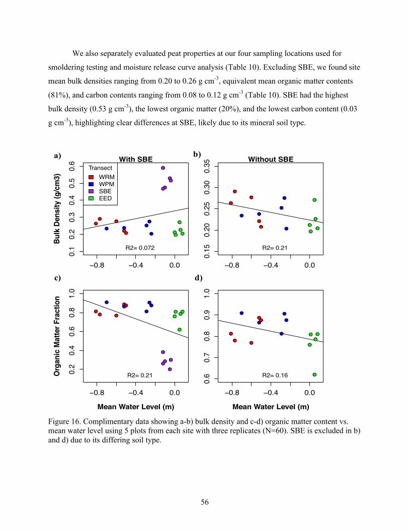
56

We also separately evaluated peat properties at our four sampling locations used for

smoldering testing and moisture release curve analysis (Table 10). Excluding SBE, we found site

mean bulk densities ranging from 0.20 to 0.26 g cm-3, equivalent mean organic matter contents

(81%), and carbon contents ranging from 0.08 to 0.12 g cm-3 (Table 10). SBE had the highest

bulk density (0.53 g cm-3), the lowest organic matter (20%), and the lowest carbon content (0.03

g cm-3), highlighting clear differences at SBE, likely due to its mineral soil type.

Figure 16. Complimentary data showing a-b) bulk density and c-d) organic matter content vs. mean water level using 5 plots from each site with three replicates (N=60). SBE is excluded in b) and d) due to its differing soil type.

a)

c) d)

b)

●●

●

●●

●●

●

●●

●

●●

●

●

●●

●

●

●

−0.8 −0.4 0.0

0.1

0.2

0.3

0.4

0.5

0.6

Bulk

Den

sity

(g/c

m3)

R2= 0.072

With SBETransect

WRMWPMSBEEED

●

●

●

●

●

●

●

●

●●

●

●

●

●

●

−0.8 −0.4 0.0

0.15

0.20

0.25

0.30

0.35

R2= 0.21

Without SBE

●● ●

●●

●

●●●

●

●

●

●

●●

●●

●

●

●

−0.8 −0.4 0.0

0.2

0.4

0.6

0.8

1.0

Mean Water Level (m)

Orga

nic

Mat

ter F

ract

ion

R2= 0.21

●

●●

●●

●

●

●●

●

●●

●

●

●

−0.8 −0.4 0.0

0.6

0.7

0.8

0.9

1.0

Mean Water Level (m)

R2= 0.16

57

Table 10. Mean (standard deviation) bulk density, organic fraction, carbon content, and mean water level at the four sampling locations used in smoldering testing and moisture release curve analysis.

Site Bulk Density

(g/cm3) Organic Fraction

(g/g) Carbon Content

(g/cm3) Mean Water Level

(m)

WRM 0.26 (0.03) 0.81 (0.03) 0.11 (0.01) -0.81 (0.35) WPM 0.25 (0.02) 0.81 (0.06) 0.12 (0.003) -0.29 (0.26) SBE 0.53 (0.01) 0.20 (0.02) 0.03 (0.02) -0.05 (0.28) EED 0.20 (0.02) 0.81 (0.02) 0.08 (0.003) 0.01 (0.09)

3.4.2 Smoldering Thresholds

Using 18 samplings at each site, ignition testing yielded 18 binary responses of burn (1)

or no burn (0) per site. With these data, we developed site-specific logistic relationships to

predict burn probability (%) at a given moisture content (Figure 17, Table 11). Using the

gravimetric moisture content value at 50% burn probability (GMCburn), we compared sites by

wetness and soil properties. As expected, at WRM, WPM, and EED, we found increasing

GMCburn (Table 11) with increased mean water level and decreased bulk density; that is, the

wettest site (EED) was most vulnerable to ignite and burn at the highest gravimetric moisture

content (290%). SBE had the lowest GMCburn (i.e., it requires drier conditions to burn),

concordant with its highest bulk density and lowest organic matter content.

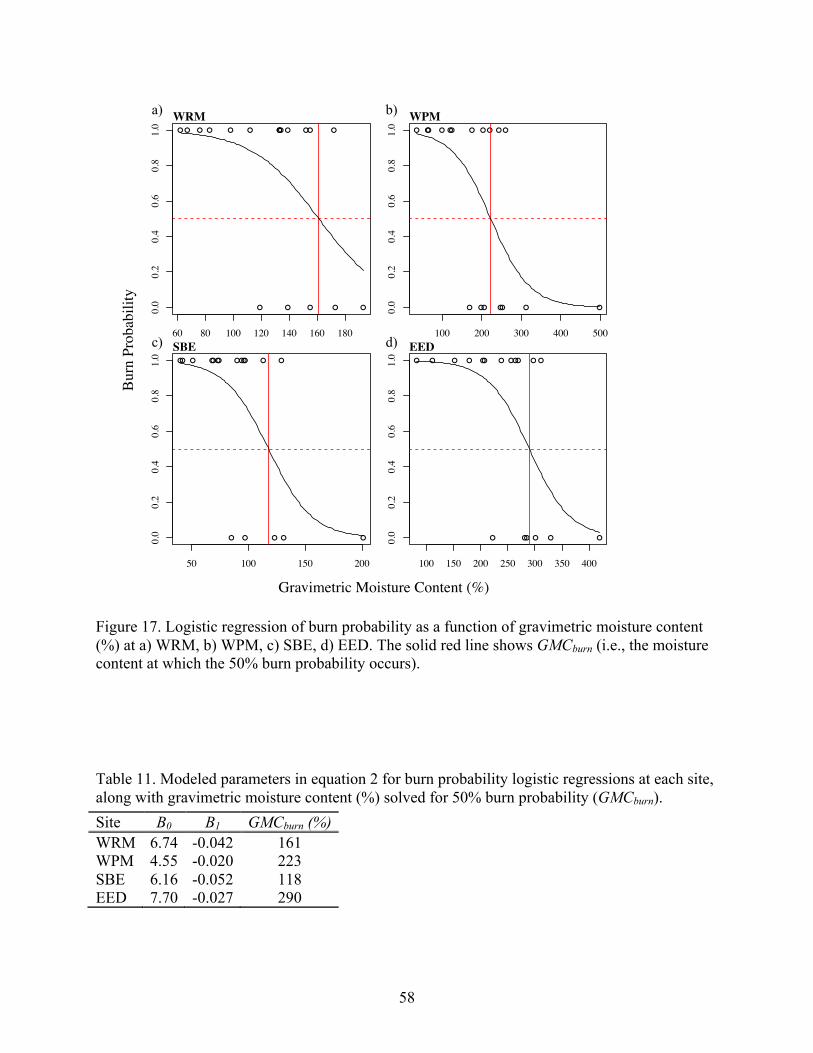
58

Figure 17. Logistic regression of burn probability as a function of gravimetric moisture content (%) at a) WRM, b) WPM, c) SBE, d) EED. The solid red line shows GMCburn (i.e., the moisture content at which the 50% burn probability occurs). Table 11. Modeled parameters in equation 2 for burn probability logistic regressions at each site, along with gravimetric moisture content (%) solved for 50% burn probability (GMCburn). Site B0 B1 GMCburn (%) WRM 6.74 -0.042 161 WPM 4.55 -0.020 223 SBE 6.16 -0.052 118 EED 7.70 -0.027 290

●

●

●

●●● ●●

●●●

● ●● ●● ●●

60 80 100 120 140 160 180

0.0

0.2

0.4

0.6

0.8

1.0

df1$gmc

df1$

burn

WRM●

●●

●●●●● ●

●● ●

●

●●

●●●

100 200 300 400 500

0.0

0.2

0.4

0.6

0.8

1.0

df2$gmcdf

2$bu

rn

WPM

●●●

●●● ●●

●

● ●● ●● ● ● ●

●

50 100 150 200

0.0

0.2

0.4

0.6

0.8

1.0

df3$gmc

df3$

burn

SBE

●●●

●●●●● ●

●

● ●●●

●

● ●

●

100 150 200 250 300 350 400

0.0

0.2

0.4

0.6

0.8

1.0

df4$gmc

df4$

burn

EED

Gravimetric Moisture Content (%)

Bur

n Pr

obab

ility

a) b)

c) d)

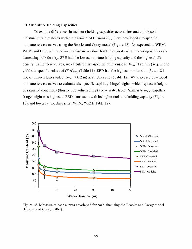
59

3.4.3 Moisture Holding Capacities

To explore differences in moisture holding capacities across sites and to link soil

moisture burn thresholds with their associated tensions (hburn), we developed site-specific

moisture release curves using the Brooks and Corey model (Figure 18). As expected, at WRM,

WPM, and EED, we found an increase in moisture holding capacity with increasing wetness and

decreasing bulk density. SBE had the lowest moisture holding capacity and the highest bulk

density. Using these curves, we calculated site-specific burn tensions (hburn; Table 12) required to

yield site-specific values of GMCburn (Table 11). EED had the highest burn tension (hburn = 8.1

m), with much lower values (hburn < 0.2 m) at all other sites (Table 12). We also used developed

moisture release curves to estimate site-specific capillary fringe heights, which represent height

of saturated conditions (thus no fire vulnerability) above water table. Similar to hburn, capillary

fringe height was highest at EED, consistent with its higher moisture holding capacity (Figure

18), and lowest at the drier sites (WPM, WRM; Table 12).

Figure 18. Moisture release curves developed for each site using the Brooks and Corey model (Brooks and Corey, 1964).

0

50

100

150

200

250

300

350

400

450

500

0 10 20 30 40 50

Moi

stur

e C

onte

nt (%

)

Water Tension (m)

WRM_Observed

WRM_Modeled

WPM_Observed

WPM_Modeled

SBE_Observed

SBE_Modeled

EED_Observed

EED_Modeled

60

Table 12. Model parameters in equation 4 for moisture release curves at each site along with the tensions (hburn) for soil moisture burn thresholds at 50% probability and estimated capillary fringe heights (CF; via eq. 5).

Site Θsat (%) λ hb (m) hburn (m) CF (m)

WRM 226 0.0749 0.0021 0.1941 0.0038 WPM 326 0.0893 0.0012 0.0877 0.0022 SBE 175 0.1402 0.0472 0.8117 0.0805 EED 441 0.1353 0.3545 8.083 0.6066

3.4.4 Uncertainty and Site Comparisons of Burn Vulnerability

Using our developed equations from the smoldering tests (logistic regressions) and

moisture release curves (Brooks and Corey model), we solved for burn threshold values for both

GMCburn and hburn at each site. We resampled equation parameters within 90% confidence

intervals to estimate uncertainty around threshold values (Figure 19). Uncertainty was largely

due to the logistic regressions, which then propagated through the hburn values (i.e., moisture

release curve equations had less parameter uncertainty). Given these uncertainties, EED and

WPM had the highest burn GMCburn values suggesting highest burn vulnerability when

considering soil moisture alone (Figure 19). However, when also considering moisture holding

capacity, EED had the highest hburn value, indicating higher required tension for burn and thus a

lower burn vulnerability. The hburn threshold describes the required water table depth to reach

GMCburn, while assuming hydrostatic equilibrium. As such, we calculated percent time each

site’s water levels were below such water table depth thresholds (via site mean hburn values) over

the 16-month observation period. Because hydrostatic equilibrium does not necessarily occur in

the field, we also calculated the proportion of time that water levels at each site were below

capillary fringe heights, representing an alternative (and more conservative) estimate of temporal

burn probability. WRM water levels were always lower than both thresholds (hburn and capillary

fringe heights; Table 13), suggesting it was always at risk to burn. In contrast, EED water levels

were always higher than both thresholds, suggesting the site was never at risk to burn. WPM and

SBE intermittently experienced water levels crossing both thresholds. Differences in temporal

variation in burn vulnerability (via water level below site-specific hburn) across sites are clearly

demonstrated in Figure 20.

61

Figure 19. Comparison of mean burn threshold moisture content (GMCburn) and burn tension (hburn) across sites along with estimated uncertainty using 1000 simulations (shown with error bars for 1 standard deviation). Table 13. Percent time that water levels (WL) at each site were below the thresholds for capillary fringe heights (CF) and burn tension (hburn).

WRM WPM SBE EED Time WL < CF (%) 100 86 32 0 Time WL < hburn (%) 100 79 4 0

Incr

easi

ng B

urn

Vul

nera

bilit

y

Dec

reas

ing

Bur

n V

ulne

rabi

lity

WRM WPM SBE EED

GM

Cbu

rn (%

)

0

100

200

300

400

0

2.2

4.4

6.6

8.8

11

h bur

n (m

)

62

Figure 20. Time series of sub-daily water levels at a) WRM, b) WPM, c) SBE, d) EED. Orange shading indicates periods when water levels were below the site-specific burn threshold (hburn ) and vulnerable to burn. Dashed black line denotes ground surface.

−1.5

−1.0

−0.5

0.0

df$time

Wat

er L

evel

[m]

−1.5

−1.0

−0.5

0.0

df$time

Wat

er L

evel

[m]

−1.5

−1.0

−0.5

0.0

df$time

Wat

er L

evel

[m]

−1.5

−1.0

−0.5

0.0

df$time

Wat

er L

evel

[m]

Apr May Jun Jul Aug Sep Oct Nov Dec Jan Feb Mar Apr May Jun Jul

a) WRM

b) WPM

c) SBE

d) EED

63

3.5 Discussion In this work, we sought to explore hydrologic controls on peat fire vulnerability, testing

two hypotheses:

H3) Long-term hydrologic regime influences peat properties (bulk density, organic matter, and moisture holding capacity) that together create variation in fire vulnerability across sites.

H4) Increased wetness will decrease fire vulnerability through integrated effects of site- specific soil moisture burn thresholds, moisture holding capacity, and water level dynamics.

To first explore hydrologic controls on peat fire, we used evaluated relationships between

mean water level and peat properties thought to influence fire vulnerability. To do so, we used a

larger complimentary dataset spanning 20 locations varying in hydrologic regime. As expected

(H3), with the exception of SBE, bulk density decreased with increased wetness (Figure 16b),

consistent with previous work (Chambers et al., 2011). In contrast, we found decreasing organic

matter content with increased wetness when removing SBE (Figure 16d). However, this negative

correlation with wetness was weak and highly leveraged by one outlier at EED; removing this

outlier results in a non-significant relationship (data not shown), suggesting other possible

influences (e.g., quantity or lability of vegetation inputs; Chambers et al., 2011). Soil type at

SBE (see Table 9) clearly differed from the other sites, with higher bulk density and lower

organic matter content. At WRM, WPM, and EED, bulk densities ranged between 0.18 to 0.29 g

cm-3, and organic matter ranged from 75% to 85%, similar to global peatland ranges (bulk

density = 0.02 to 0.3 g cm-3; organic matter = 50 to 100%; Verry et al., 2011). At just our

sampling locations for smoldering and moisture holding capacity analysis (only one per site),

WRM, WPM, and EED samples had similar organic matter content (all with mean of 81%) and

(slightly) decreasing bulk density with wetness. Although we did not capture a large gradient in

soil properties across these three sites, the endmember of SBE afforded important insights

regarding peat property controls on fire vulnerability. Specifically, SBE had the highest mineral

content, lowest organic matter content, and highest bulk density.

Burn vulnerability is often quantified via soil moisture burn thresholds, which help to

document variability across sites and how peat properties influence such variability. Across our

sites, soil moisture burn thresholds for 50% burn probability (GMCburn) clearly varied (Table

11). EED had the highest GMCburn (290%), while SBE had the lowest (118%). A high GMCburn

64

suggests EED would burn even when very wet, which comports with its high organic content and

low bulk density. Alternatively, SBE may not ignite until a much lower moisture content is

reached, due to its high mineral content and bulk density. Comparing these two sites alone, the

trend of decreased fire vulnerability (via soil moisture burn thresholds) with increased mineral

content and bulk density is consistent with our prediction (H3) and other studies (Hartford, 1993;

Frandsen, 1997; Reardon et al., 2007; Benscoter et al., 2011). Excluding SBE, the other three

sites had similar organic matter content but decreasing bulk density with wetness (Table 10);

across these sites, the expected negative relationship between bulk density and fire vulnerability

was also observed (Table 11).

Soil moisture burn thresholds widely vary across systems and studies. Similar to our

findings, Reardon et al. (2007) found GMCburn values in southeastern USA peat soils between

140 to 240%. In hardwood swamp soils with similar mineral content as our study (~20%),

Frandsen (1997) found a GMCburn of 76%, lower than our observed ranges and values in Reardon

et al. (2007). Differences in studies are likely due to method variation. Our developed approach

was conservative, in that a burn/no burn response was determined only 5 minutes after the heat

source was removed, neither waiting for the sample to be consumed nor measuring consumption.

Nonetheless, the consistent method applied across our sites documented clear relative differences

in GMCburn within one peatland system. Notably, most studies have focused on differences

across regional peatland systems. Our findings emphasize that local variation should be

addressed both in future work and in fire prediction protocols. For example, fire prediction at

GDS currently relies on soil moisture monitoring using one system-wide soil moisture threshold

that identifies fire risk (F. Wurster, GDS Hydrologist, personal communication). More work at

GDS, and in other peatland systems, should seek site-specific relationships between easily

measured parameters (e.g., bulk density) and soil moisture burn thresholds to better inform such

fire risk monitoring. Our work was limited in sampled locations and in the resulting range of

mineral contents and bulk densities, highlighting future research needs at GDS.

While soil moisture burn thresholds varied across sites, site variation in moisture holding

capacity together with variation in soil moisture burn thresholds determines the required

antecedent wetness for fire vulnerability. To quantify moisture holding capacity, we developed

moisture release curves, allowing comparison of moisture contents between sites at the same

water tension and showing clear site differences in moisture holding capacity (Figure 18). EED

65

had the highest moisture holding capacity, while SBE had the lowest, comporting with bulk

density differences and supporting H3. Comparing GMCburn alone to indicate fire vulnerability

suggests that EED would burn at the highest soil moistures, followed by WPM, WRM, and SBE

(Table 11; Figure 17). However, by taking site-specific GMCburn values and estimating the water

tension (hburn) required to create those moisture contents (via moisture release curves), site

differences in fire vulnerability substantially changed. EED had the highest hburn value,

indicating that EED requires the deepest water tables to reach its GMCburn threshold (Figure 19)

and critically underscoring the need to consider both soil moisture thresholds and moisture

holding capacities. To improve confidence in our estimated thresholds (see error bars in Figure

19), more samples per site should be tested to reduce uncertainty in logistic regression

relationships. Moreover, additional tension measurements should be taken at lower (< 3 m)

tensions to better parameterize moisture release curves within ranges of hburn tensions.

To integrate both short- and long-term hydrologic effects on burn vulnerability, we

evaluated water level time series at each site, identifying times when water tables crossed two

different thresholds of fire vulnerability: hburn and capillary fringe hight (Table 13; Figure 20).

The former assumes hydrostatic equlibrium, which is often not the case due to diurnally varying

inputs/outputs of soil moisture (e.g., precipitation, evapotranspiration; Brady and Weil, 2008).

As such, we included capillary fringe heights as an alternative and more conservative threshold.

Supporting H4, we found that burn temporal probablities using both thresholds decreased with

wetness (Table 13). Our findings suggest that WRM was always at risk to burn, while EED

maintained saturated conditions at surface (via capillary fringe) and thus never reached

conditions of burn vulnerability. Notably, these predictions integrate site-specific soil moisture

burn thresholds, moisture holding capacities, and water level dyanmics.

Our work points to research needs at GDS and temperate peatlands in general. More

specifically, at GDS, additional study sites are needed to better link measured peat parameters to

soil moisture burn thresholds and burn tensions. Such information is important to adjust now

constant soil moisture burn thresholds used across GDS locations for fire risk warning. More

broadly, research is needed to better address the hydrologic controls on peat properties that

influence soil moisture burn thresholds, but especially those that influence tensions required to

reach such thresholds. Critically, this role of moisture holding capacity is not currently

recognized. Ultimately, research should seek predictive models that couple water level

66

monitoring and measured soil parameters to predict surface peat fire vulnerability over both time

and space.

Conclusions

Our findings highlight long-term hydrologic influences on peat properties that in turn

influence peat fire vulnerability as a function of daily water level dynamics. As such, research

findings will help inform both hydrologic restoration and fire monitoring at GDS and, more

broadly, advance our understanding of integrated interactions among hydrologic regime, peat

properties, and fire vulnerability in temperate peatlands.

67

Literature Cited Atkinson, R. B., J. W. DeBerry, D. T. Loomis, E. R. Crawford, R. T. Belcher, R. B. Atkinson, R.

T. Belcher, D. A. Brown, and J. E. Perry. 2003. Water Tables in Atlantic White Cedar Swamps: Implications for Restoration. In Atlantic White Cedar Restoration Ecology and Management, Proceedings of a Symposium. Christopher Newport University, Newport News, 137–150.

Benscoter, B. W., D. K. Thompson, J. M. Waddington, M. D. Flannigan, B. M. Wotton, W. J. De Groot, and M. R. Turetsky. 2011. Interactive Effects of Vegetation, Soil Moisture and Bulk Density on Depth of Burning of Thick Organic Soils. International Journal of Wildland Fire 20, 3: 418–429.

Boelter, D. H. 1968. Important Physical Properties of Peat Materials.

Brady, N. C., and R. R. Weil. 2008. The Nature and Properties of Soils. 14th ed. Prentice-Hall Inc. Upper Saddle River, New Jersey.

Brooks, R. H., and A. T. Corey. 1964. Hydraulic Properties of Porous Media and Their Relation to Drainage Design. Trans. ASAE 7, 1: 26–28.

Casey, W. P., and K. C. Ewel. 2006. Patterns of Succession in Forested Depressional Wetlands in North Florida, USA. Wetlands 26, 1: 147–160.

Chambers, F.M., D.W. Beilman, and Z Yu. 2011. Methods for Determining Peat Humification and for Quantifying Peat Bulk Density, Organic Matter and Carbon Content for Palaeostudies of Climate and Peatland Carbon Dynamics.” Mires and Peat 7, 7: 1–10.

Dane, J. H., and J. W. Hopmans. 2002. 3.3.2.4 Pressure Plate Extractor. Methods of Soil Analysis: Part 4 Physical Methods, 671–973.

Francis, H. E. 1959. Soil Survey for Norfolk County, Virginia, 53.

Frandsen, W. H. 1987. The Influence of Moisture and Mineral Soil on the Combustion Limits of Smoldering Forest Duff. Canadian Journal of Forest Research 17, 12: 1540–1544.

Frandsen, W. H. 1997. Ignition Probability of Organic Soils 27, 1471–1477.

Gorham, E. 1991. Northern Peatlands: Role in the Carbon Cycle and Probable Responses to Climatic Warming. Ecological Applications 1, 2: 182–195.

Hartford, Roberta A. 1993. Smoldering Combustion Limits in Peat as Influenced by Moisture Mineral Content and Organic Bulk Density.

Hugron, S., J. Bussières, and L. Rochefort. 2013. Tree Plantations within the Context of Ecological Restoration of Peatlands: Practical Guide. Peatland Ecology Research Group, Université Laval, Québec, Québec, Canada.

Legrand Jr, H. E. 2000. The Natural Features of Dismal Swamp State Natural Area, North Carolina. The Natural History of the Great Dismal Swamp, Omni, Madison, Wisconsin, 41–50.

Levy, G. F. 1991. The Vegetation of the Great Dismal Swamp: A Review and an Overview. Virginia Journal of Science 42, 4: 411–418.

68

Lichtler, W., F., and P. Walker. 1974. Hydrology of the Dismal Swamp, Virginia-North Carolina. Geological Survey - Water Resources Division, no. 74–39.

Osborn, C. C. 1919. Peat in the Dismal Swamp, Virginia and North Carolina. Contribution to Economic Geology Bull 711, 4.

Page, S. E., J. O. Rieley, ØW Shotyk, and D. Weiss. 1999. Interdependence of Peat and Vegetation in a Tropical Peat Swamp Forest. Philosophical Transactions of the Royal Society of London B: Biological Sciences 354, 1391: 1885–1897.

Page, S. E., F. Siegert, J. O. Rieley, H. V. Boehm, A. Jaya, and S. Limin. 2002. The Amount of Carbon Released from Peat and Forest Fires in Indonesia during 1997. Nature 420, 6911: 61–65.

Phipps, R. L., D. L. Ierley, and C. P. Baker. 1979. Tree Rings as Indicators of Hydrologic Change in the Great Dismal Swamp, Virginia and North Carolina. US Geological Survey, Water Resources Division.

Poulter, B., N. L. Christensen, and P. N. Halpin. 2006. Carbon Emissions from a Temperate Peat Fire and Its Relevance to Interannual Variability of Trace Atmospheric Greenhouse Gases. Journal of Geophysical Research: Atmospheres 111, D6.

R Core Team. 2016. R: A Language and Environment for Statistical Computing. Vienna, Austria: R Foundation for Statistical Computing.

Raats, P. A. C., and W. R. Gardner. 1971. Comparison of Empirical Relationships between Pressure Head and Hydraulic Conductivity and Some Observations on Radially Symmetric Flow. Water Resources Research 7, 4: 921–928.

Reardon, J., R. Hungerford, and K. Ryan. 2007. Factors Affecting Sustained Smouldering in Organic Soils from Pocosin and Pond Pine Woodland Wetlands. International Journal of Wildland Fire 16, 1: 107–118.

Reddy, A. D., T. J. Hawbaker, F. Wurster, Z. Zhu, S. Ward, D. Newcomb, and R. Murray. 2015. Quantifying Soil Carbon Loss and Uncertainty from a Peatland Wildfire Using Multi-Temporal LiDAR. Remote Sensing of Environment 170: 306–316.

Rein, G., N. Cleaver, C. Ashton, P. Pironi, and J. L. Torero. 2008. The Severity of Smouldering Peat Fires and Damage to the Forest Soil. Catena 74, 3: 304–309.

Shimada, S., H. Takahashi, A. Haraguchi, and M. Kaneko. 2001. The Carbon Content Characteristics of Tropical Peats in Central Kalimantan, Indonesia: Estimating Their Spatial Variability in Density. Biogeochemistry 53, 3: 249–267.

Sorensen, K. W. 1993. Indonesian Peat Swamp Forests and Their Role as a Carbon Sink. Chemosphere 27, 6: 1065–1082.

Turetsky, M. R., B. Benscoter, S. Page, G. Rein, G. R. van der Werf, and A. Watts. 2015. Global Vulnerability of Peatlands to Fire and Carbon Loss. Nature Geoscience 8, 1: 11–14.

Usup, A. Y. Hashimoto, H. Takahashi, and H. Hayasaka. 2004. Combustion and Thermal Characteristics of Peat Fire in Tropical Peatland in Central Kalimantan, Indonesia. Tropics 14, 1: 1–19.

69

Verry, E. S., D. H. Boelter, J. Päivänen, D. S. Nichols, T. Malterer, and A. Gafni. 2011. Physical Properties of Organic Soils. Peatland Biogeochemistry and Watershed Hydrology at the Marcell Experimental Forest (Eds Kolka RK, Sebestyen SD, Verry ES, Brooks KN), 135–176.

Watts, A. C., and L. N. Kobziar. 2013. Smoldering Combustion and Ground Fires: Ecological Effects and Multi-Scale Significance. Fire Ecol 9, 1: 124–32.

Watts, A. C., C. A. Schmidt, D. L. McLaughlin, and D. A. Kaplan. 2015. Hydrologic Implications of Smoldering Fires in Wetland Landscapes. Freshwater Science 34, 4: 1394–1405.

70

4.0 HYDROLOGIC RESTORATION OF ECOSYSTEM STRUCTURE AND FUNCTION IN THE GREAT DISMAL SWAMP

Hydrologic restoration is coming to GDS in 2016-2017 with the management objectives

to increase species diversity, increase carbon storage via peat depth, and decrease fire

vulnerability. Our third objective was to inform hydrologic restoration of ecosystem structure

and function in GDS. To do so, we conducted two complimentary studies to test developed

hypotheses regarding hydrologic influences on vegetation, peat depths, and peat fire

vulnerability.

In our first study, we explored hydrologic controls on peat depth, microtopography, and

vegetation composition. At higher water levels, we expected (H1) peat to be deepest and

microtopography to be most variable. We also expected (H2) that red maple would be less

competitive at higher mean water levels, thus increasing tree diversity and desired species (e.g.,

cedar, cypress, tupelo) abundance. We tested these hypotheses by coupling in situ hydrologic

monitoring with peat, elevation, and vegetation surveys along a gradient of wetness both at the

transect and plot level. We found evidence to support H1 and H2. Specifically, at sites of

increased wetness (e.g., higher water levels), we found: 1) thicker peat and more

microtopographic variation; 2) lower maple importance; and 3) higher tree species richness.

In our second study, we examined hydrologic controls on peat fire vulnerability and

associated peat properties. We expected (H3) long-term hydrologic regime to influence peat

properties (bulk density, mineral content, and moisture holding capacity) that collectively

determine site variation in fire vulnerability. We also expected (H4) increased wetness to

decrease fire vulnerability through integrated effects of site-specific soil moisture burn

thresholds, moisture holding capacity, and water level dynamics. We measured in situ water

level data, peat properties, burn probability as a function of soil moisture, and moisture holding

capacity at four sites. Due to differences in soils (more mineral-rich), one site (SBE) served as an

endmember in our analyses and is excluded from the following conclusions. We found that

wetter sites burn at higher soil moistures but also have higher moisture holding capacities,

supporting H3. Burn tension (i.e., hburn; tension necessary to create site-specific soil moisture

burn thresholds) is a better representation of how soil moisture and thus smoldering fire

71

vulnerability is realized in the field. Through integrated analysis of water level time series,

capillary fringe heights, and hburn values, we compared the duration (%) that each site was at risk

to ignition. Burn vulnerability decreased with wetness (supporting H4), suggesting that the driest

site (WRM) was always at risk to burn, and the wettest (EED) never approached conditions for

ignition vulnerability.

Together, findings from these two studies demonstrate strong hydrologic controls on

GDS ecosystem structure and function. As such, results can be used to begin informing water

level management for specific restoration goals. Critically, this research also provides baseline

data for comparison with post-restoration monitoring to empirically evaluate the effects of

hydrologic restoration on peat depth, microtopography, and vegetation composition. Going

forward, continued research across more GDS locations should focus on hydrology-vegetation

interactions and spatial variation in burn vulnerability, ultimately guiding adaptive management

and restoration in the Swamp.