HYDROGEOMORPHIC WETLAND PROFILING: AN APPROACH …Hydrogeomorphic Wetland Profiling (HGM WP), seeks...
106
United States National Health and Environmental EPA/620/R-05/001 Environmental Effects Research Laboratory January 2005 Protection Agency Corvallis, OR 97333 HYDROGEOMORPHIC WETLAND PROFILING: AN APPROACH TO LANDSCAPE AND CUMULATIVE IMPACTS ANALYSIS Environmental Monitoring and Assessment Program
Transcript of HYDROGEOMORPHIC WETLAND PROFILING: AN APPROACH …Hydrogeomorphic Wetland Profiling (HGM WP), seeks...
United States National Health and Environmental EPA/620/R-05/001Environmental Effects Research Laboratory January 2005Protection Agency Corvallis, OR 97333
HYDROGEOMORPHIC WETLAND PROFILING: AN APPROACHTO LANDSCAPE AND CUMULATIVE IMPACTS ANALYSIS
Environmental Monitoring and Assessment Program


EPA/620/R-05/001January 2005
HYDROGEOMORPHIC WETLAND PROFILING:AN APPROACH TO LANDSCAPE AND
CUMULATIVE IMPACTS ANALYSIS
By
J. Bradley JohnsonDepartment of Biology
Colorado State UniversityFort Collins, CO 80523
NATIONAL HEALTH AND ENVIRONMENTAL EFFECTS RESEARCH LABORATORYOFFICE OF RESEARCH AND DEVELOPMENT
U.S. ENVIRONMENTAL PROTECTION AGENCYRESEARCH TRIANGLE PARK, NC 27711
i
NOTICE
This report was funded wholly by the U.S. Environmental Protection Agency (EPA)under Cooperative Agreement number R-82843901 to the Colorado Geological Survey. Theresearch reported herein was conducted in collaboration with the EPA’s EnvironmentalMonitoring and Assessment Program (EMAP) and the Regional Applied Research Effort(RARE) Program.
This report has been subjected to review by the EPA National Health and EnvironmentalEffects Research Laboratory’s Western Ecology Division and approved for publication. Approval does not signify that the contents reflect the views of the Agency, nor does mention oftrade names or commercial products constitute endorsement or recommendation for use.
The correct citation for this document is:
Johnson, J. Bradley. 2005. Hydrogeomorphic Wetland Profiling: An Approach to Landscapeand Cumulative Impacts Analysis. EPA/620/R-05/001. U.S. Environmental Protection Agency,Washington, D.C.

ii
ACKNOWLEDGMENTS
Many people contributed their time and expertise to this project. Foremost, I would like to thank Richard Sumner of US Environmental Protection Agency’s (EPA) Office of Researchand Development (ORD), who truly made this project possible and who generously provideduntold hours of advice, support, and insightful conversation. Mary E. Kentula of EPA ORD alsowas unfaltering in her assistance, offering key insights, excellent suggestions, and editorialexpertise during project development and finalization. The efforts of D. Noe and the ColoradoGeological were essential to this project and much appreciated. My thanks to D. Steingraeberfor his continued collaboration. I would like to thank R. McEldowney of Science ApplicationsInternational Corporation, who supplied invaluable wetlands data and classified the majority ofwetlands into HGM classes. Summit County government, and H. McLaughlin were generouswith both their time and resources, and their contribution is greatly appreciated. Finally, I wouldlike to thank the participants who attended a workshop held at EPA Region 8's Denver office andwho significantly aided in the conceptualization of this project, including (but not limited to) B.Bedford, D. Smith, S. Leibowitz, D. Noe, M. Claffey, D. Patten, G. Reetz, W. Schweiger, and G.Rodriguez.

iii

iv
TABLE OF CONTENTS
NOTICE . . . . . . . . . . . . . . . . . . . . . . . . . . . . . . . . . . . . . . . . . . . . . . . . . . . . . . . . . . . . . . . . . . . . . i
ACKNOWLEDGMENTS . . . . . . . . . . . . . . . . . . . . . . . . . . . . . . . . . . . . . . . . . . . . . . . . . . . . . . ii
EXECUTIVE SUMMARY . . . . . . . . . . . . . . . . . . . . . . . . . . . . . . . . . . . . . . . . . . . . . . . . . . . . . vi
INTRODUCTION . . . . . . . . . . . . . . . . . . . . . . . . . . . . . . . . . . . . . . . . . . . . . . . . . . . . . . . . . . . . . 1Theoretical Basis for Approach . . . . . . . . . . . . . . . . . . . . . . . . . . . . . . . . . . . . . . . . . . . . . 1Background on HGM WP Development . . . . . . . . . . . . . . . . . . . . . . . . . . . . . . . . . . . . . . 3Extension of HGM WP to the Generalized Case of Cumulative Impacts Analysis . . . . . 4
METHODS . . . . . . . . . . . . . . . . . . . . . . . . . . . . . . . . . . . . . . . . . . . . . . . . . . . . . . . . . . . . . . . . . . 6Description of Study Area . . . . . . . . . . . . . . . . . . . . . . . . . . . . . . . . . . . . . . . . . . . . . . . . 6Development of the Geographic Information System . . . . . . . . . . . . . . . . . . . . . . . . . . . . 8Designation of Process Domains . . . . . . . . . . . . . . . . . . . . . . . . . . . . . . . . . . . . . . . . . . . 10Identification of Ecoregions . . . . . . . . . . . . . . . . . . . . . . . . . . . . . . . . . . . . . . . . . . . . . . . 11Classification of Impact Categories . . . . . . . . . . . . . . . . . . . . . . . . . . . . . . . . . . . . . . . . . 12Generation of HGM WPs and Detection of Cumulative Impacts . . . . . . . . . . . . . . . . . . 12Methodological Assumptions . . . . . . . . . . . . . . . . . . . . . . . . . . . . . . . . . . . . . . . . . . . . . 14
RESULTS . . . . . . . . . . . . . . . . . . . . . . . . . . . . . . . . . . . . . . . . . . . . . . . . . . . . . . . . . . . . . . . . . . 16Identification of Ecoregions . . . . . . . . . . . . . . . . . . . . . . . . . . . . . . . . . . . . . . . . . . . . . . . 16
Low Lands Ecoregion . . . . . . . . . . . . . . . . . . . . . . . . . . . . . . . . . . . . . . . . . . . . . 20Middle-elevation Transitional Ecoregion . . . . . . . . . . . . . . . . . . . . . . . . . . . . . . 20High Mountains Ecoregion . . . . . . . . . . . . . . . . . . . . . . . . . . . . . . . . . . . . . . . . . 20
Classification of Impact Categories . . . . . . . . . . . . . . . . . . . . . . . . . . . . . . . . . . . . . . . . . 20Use of HGM WPs to Detect Cumulative Impacts . . . . . . . . . . . . . . . . . . . . . . . . . . . . . . 24
Evaluation of Consistency of HGM WPs Within Ecoregions . . . . . . . . . . . . . . . 24Detection of Cumulative Impacts . . . . . . . . . . . . . . . . . . . . . . . . . . . . . . . . . . . . 28
DISCUSSION . . . . . . . . . . . . . . . . . . . . . . . . . . . . . . . . . . . . . . . . . . . . . . . . . . . . . . . . . . . . . . . 33Reference-based Cumulative Impacts Analysis . . . . . . . . . . . . . . . . . . . . . . . . . . . . . . . 34Landscape Characterization and Indexing of Cumulative Effects . . . . . . . . . . . . . . . . . . 35Utility and Limitations of HGM WP . . . . . . . . . . . . . . . . . . . . . . . . . . . . . . . . . . . . . . . . 37Critical Evaluation of the Method . . . . . . . . . . . . . . . . . . . . . . . . . . . . . . . . . . . . . . . . . . 40
Insensitivity to Within-Wetland Impacts . . . . . . . . . . . . . . . . . . . . . . . . . . . . . . . 40Lack of Appropriate Reference Standard Landscapes . . . . . . . . . . . . . . . . . . . . . 40Categorization of Impact Level . . . . . . . . . . . . . . . . . . . . . . . . . . . . . . . . . . . . . . 41Problematic Wetlands . . . . . . . . . . . . . . . . . . . . . . . . . . . . . . . . . . . . . . . . . . . . . 42

v
Future Applications of HGM Wetland Profiling . . . . . . . . . . . . . . . . . . . . . . . . . . . . . . . 42Conclusions . . . . . . . . . . . . . . . . . . . . . . . . . . . . . . . . . . . . . . . . . . . . . . . . . . . . . . . . . . . 43
REFERENCES CITED . . . . . . . . . . . . . . . . . . . . . . . . . . . . . . . . . . . . . . . . . . . . . . . . . . . . . . . . 45
APPENDIX 1: KEY TO SUMMIT COUNTY, COLORADO, WETLAND TYPES . . . . . . . . 53

vi
EXECUTIVE SUMMARY
Cumulative impacts and their resultant cumulative effects have become an importantfocus of both environmental regulation and scientific investigation because of their potentiallysevere consequences. For example, the National Environmental Policy Act (38 CFR Sect.1500.6) and Section 404(b)(1) of the Clean Water Act (40 CFR 230.11) explicitly require thatprojects proposing impacts to wetlands consider the cumulative effects of the actions and notsolely the direct impacts of the project. Despite the recognized potential for significant, negativeconsequences, cumulative effects are seldom sufficiently addressed in environmentalmanagement because of the lack of effective tools to describe and assess them.
This study developed a synthetic, hierarchical and scalable approach to landscapecharacterization and cumulative impacts analysis that is based on current scientific thought ofhow wetlands develop and function within landscapes. Specifically, this study investigatedwhether a reference-based approach to cumulative impacts analysis could be developed by usinga hydrogeomorphically-based version of landscape profiles (Brinson 1993, Bedford 1996, Gwinet al. 1999) in conjunction with the concepts of landscape formation and processes forwarded byMontgomery (1999), Winter (2001), and Omernik and Bailey (1997). This approach, termed Hydrogeomorphic Wetland Profiling (HGM WP), seeks to refine coarse acreage-based approaches by applying a functionally-based framework to provide a landscape-scalecharacterization of wetland resources that is useful to regulatory, management, mitigation, andconservation programs.
Most basically, HGM WP is a method of summarizing the abundance and diversity ofHGM wetland types within a given ecoregion or portion thereof. Three related applications ofthe HGM WP approach are detailed in this report, landscape characterization, cumulativeimpacts analysis, and first-order approximation of wetland-related cumulative effects.
Landscape characterizationThis research asserts that HGM WP provides a valuable means of characterizing of
landscapes with regard to their wetland component and the functions occurring within. Using afunctionally-based classification, such as HGM, to summarize the abundance and diversitywetlands provides an estimation of the potential types and magnitude of wetland functionsperformed in that landscape. For instance, a landscape with a high proportion of slope wetlandswould be expected to predominately perform the functions ascribed to slope wetlands, such asgroundwater discharge, carbon retention, and maintenance of stream base flow.
Cumulative Impacts AnalysisThe main focus of the HGM WP approach is to provide a practically implementable,
reference-based approach to wetland cumulative impacts analysis. Specifically, HGM WPquantifies impacts to the abundance and diversity of wetlands resulting from outright wetlanddestruction or functional conversion (i.e. from one HGM class to another). This analyticalfocuses stems from the idea that these whole-wetland impacts are the primary driver or “forcingfactor” of wetland functioning at the landscape scale.
vii
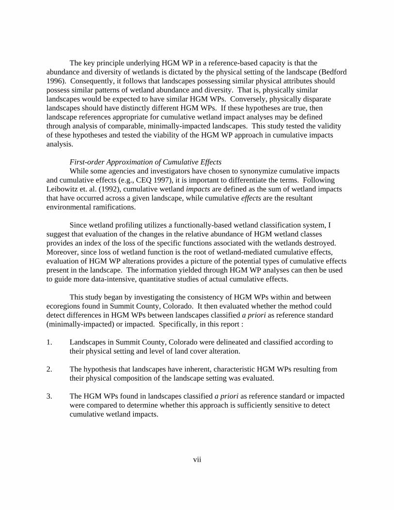
The key principle underlying HGM WP in a reference-based capacity is that theabundance and diversity of wetlands is dictated by the physical setting of the landscape (Bedford1996). Consequently, it follows that landscapes possessing similar physical attributes shouldpossess similar patterns of wetland abundance and diversity. That is, physically similarlandscapes would be expected to have similar HGM WPs. Conversely, physically disparatelandscapes should have distinctly different HGM WPs. If these hypotheses are true, thenlandscape references appropriate for cumulative wetland impact analyses may be definedthrough analysis of comparable, minimally-impacted landscapes. This study tested the validityof these hypotheses and tested the viability of the HGM WP approach in cumulative impactsanalysis.
First-order Approximation of Cumulative EffectsWhile some agencies and investigators have chosen to synonymize cumulative impacts
and cumulative effects (e.g., CEQ 1997), it is important to differentiate the terms. FollowingLeibowitz et. al. (1992), cumulative wetland impacts are defined as the sum of wetland impactsthat have occurred across a given landscape, while cumulative effects are the resultantenvironmental ramifications.
Since wetland profiling utilizes a functionally-based wetland classification system, Isuggest that evaluation of the changes in the relative abundance of HGM wetland classesprovides an index of the loss of the specific functions associated with the wetlands destroyed. Moreover, since loss of wetland function is the root of wetland-mediated cumulative effects,evaluation of HGM WP alterations provides a picture of the potential types of cumulative effectspresent in the landscape. The information yielded through HGM WP analyses can then be usedto guide more data-intensive, quantitative studies of actual cumulative effects.
This study began by investigating the consistency of HGM WPs within and betweenecoregions found in Summit County, Colorado. It then evaluated whether the method coulddetect differences in HGM WPs between landscapes classified a priori as reference standard(minimally-impacted) or impacted. Specifically, in this report :
1. Landscapes in Summit County, Colorado were delineated and classified according totheir physical setting and level of land cover alteration.
2. The hypothesis that landscapes have inherent, characteristic HGM WPs resulting fromtheir physical composition of the landscape setting was evaluated.
3. The HGM WPs found in landscapes classified a priori as reference standard or impactedwere compared to determine whether this approach is sufficiently sensitive to detectcumulative wetland impacts.

viii
4. The use of HGM WP as a means of first-order cumulative effects estimation wasdiscussed along with the method’s limitations and its potential for further refinement.
Summit County is located in the heart of the Rocky Mountains in central Colorado. Thecounty is characterized by rugged terrain and strong physical and biological gradients. Much ofSummit County is undeveloped, and 76% is under the management of the U.S. Forest Service. The county was partitioned into 95 process domain (sensu Montgomery 1999) sample units inwhich physical and ecological processes were internally homogeneous. Based on clusteranalysis, the 95 process domains were aggregated into three ecoregions: 1) low lands, 2) middle-elevation transitional, and 3) high mountains.
Since no data exist on actual wetland impacts that have occurred in Summit County, landuse/land cover (LULC) and road density were used to index the likelihood or severity ofcumulative wetland impacts. Process domains were classified into one of two, a priori impactcategories (reference standard or impacted) based on LULC and road density using clusteranalysis.
Two primary questions were evaluated during this study: 1) considering only minimally-impacted, reference standard landscapes, are HGM WPs relatively consistent within ecoregionsand do they differ between ecoregions?; and 2) within ecoregions, do HGM WPs statisticallydiffer between impacted and reference standard landscapes as a result of cumulative wetlandimpacts?
The results of this investigation support both hypotheses within the study area. First,HGM WPs within the study units were found to be more similar within than between ecoregions. Between ecoregions, profiles differed in overall shape or in the relative abundance of two ormore wetland classes. This result suggests that ecoregions have characteristic and discernableHGM WPs. This is a key finding since there had not been an empirical evaluation of how tightlythe abundance and diversity of wetlands is tied to the physical setting. Because of thedemonstrated linkage between physical setting and HGM WP, this approach provides a plausiblemeans of reference-based cumulative impacts analysis.
Comparison of reference standard and impacted landscape units (process domains) withinecoregions showed that profile alterations could be statistically detected. Profile differenceswere manifested as an overall change in profile shape or in an alteration in the ratio between twoor more wetland classes. Changes to HGM WPs in impacted landscapes could be readily tied tocurrent and historical land use patterns.
These findings show that HGM WP is a promising method with which to characterizecumulative wetland impacts. Further, as a result of its design, HGM WP results can be combinedwith data derived through smaller-scale approaches to yield multi-scale analyses of wetlandresources. The method also seems a useful means of addressing additional facets of landscape

ix
analysis of wetlands, including wetland-based landscape classification, threshold detection, andsynoptic analyses.
The report is presented in four major sections. The first is this executive summary whichoutlines the project’s approach and major findings. The second provides an introduction to theconcepts underlying hydrogeomorphic wetland profiling including background on the regulatoryand scientific context of the method. In the third section, a generalized approach to HGM WP isdescribed, implemented, and tested in Summit County, Colorado. Lastly, a tool for remotelyclassifying wetlands is provided as an appendix.

1
INTRODUCTION
Cumulative impacts and their resultant cumulative effects have become an importantfocus of both environmental regulation and scientific investigation because of their potentiallysevere consequences. For example, the National Environmental Policy Act (38 CFR Sect.1500.6) and Section 404(b)(1) of the Clean Water Act (40 CFR 230.11) explicitly require thatprojects proposing impacts to wetlands consider the cumulative effects of the actions and notsolely the direct project impacts. Despite the recognized potential for significant negativeconsequences, cumulative effects are seldom adequately addressed in environmentalmanagement because of the lack of effective tools to describe and assess them. The purpose ofthe research documented in this report was to explore how recent, innovative concepts inwetland ecology could be integrated to create a practical and powerful approach to wetlandcumulative impacts analysis.
Specifically, this study investigated whether a reference-based approach to cumulativeimpacts analysis could be developed by using a hydrogeomorphically-based version of landscapeprofiles (Brinson 1993, Bedford 1996, Gwin et al. 1999) in conjunction with the concepts oflandscape formation and processes forwarded by Montgomery (1999), Winter (2001), andOmernik and Bailey (1997). This approach, termed Hydrogeomorphic Wetland Profiling (HGMWP), seeks to refine coarse acreage-based approaches by applying a functionally-basedframework that provides the landscape-scale view of wetland resources needed by regulatory,management, mitigation, and conservation programs.
Theoretical Basis for ApproachScientific investigations have shown that wetlands unquestionably perform important
environmental functions (National Research Council [NRC] 1995, Mitsch and Gosselink 2000)and that different types of wetlands perform different functions or the same functions to variousdegrees (e.g., Brinson 1993, NRC 1995). Thus, with loss and degradation of wetlands comes aconcomitant loss of functions generally associated with wetlands and the particularenvironmental functions attributed to specific wetland types. The functional losses result in bothdirect and indirect negative effects on environmental quality such as impairment of waterquality, reduction of flood flow attenuation, and loss of wildlife habitat (Hemond and Benoit1988, Croonquist and Brooks 1991, Council on Environmental Quality [CEQ] 1997, Bedford

2
1999, McAllister et al. 2000, NRC 2001). When taken singly, any particular wetland impactmay have little effect on overall environmental quality. But considering whole watersheds andbasins, the cumulative sum of wetland impacts may have significant additive effects, or wetlandimpacts can act synergistically to produce disproportionately severe cumulative effects (Hemondand Benoit 1988, Nestler and Long 1997).
While some agencies and investigators have chosen to synonymize cumulative impactswith cumulative effects (e.g., CEQ 1997), it is important to differentiate the terms. FollowingLeibowitz et. al. (1992), cumulative wetland impacts are defined as the sum of extant andhistorical wetland impacts that have occurred across a given landscape, while cumulative effectsare the resultant environmental consequences. Cumulative wetland impacts can take the form ofoutright destruction of wetland habitat, of functional conversion (e.g., converting riparianwetlands to depressions), or of a decline in wetland functioning through mechanisms such assedimentation, hydrologic alteration, or logging. Alternatively, the cumulative effects ofwetland loss are manifested as a degradation of environmental quality. One way of contrastingcumulative wetlands impacts with cumulative effects, is that cumulative wetland impacts alwaysoccur within wetlands across a landscape, while cumulative effects are commonly manifestedoutside of wetland ecosystems, in receiving waters.
Analysis of wetland acreage trends is the most basic method of characterizing cumulativewetland impacts. Such analyses provide data on wetland losses (or gains) and thereby providean indication of the general types of ecosystem functions that have been lost within the studyregion. While an important means of tracking broad environmental trends, such an approachsuffers from its inherent generality and insensitivity to differential wetland functioning, and itdoes not provide the level of detail necessary for smaller-scale regional studies. These short-comings are especially significant in light of the non-random distribution of wetland impacts(Bedford 1999), which make accurate predictions about wetland-related functional losses andcumulative effects unlikely.
The information rendered through trend analyses can be greatly increased by stratifying surveyed wetlands into discrete categories. Wetland classifications can be structured around anygroup of parameters, but recent studies suggest that hydrogeomorphic (HGM) classification(Brinson 1993) is particularly powerful because of its physical basis and its direct ties to wetland

1 Although Bedford applied the term “landscape profiling”, I will instead use the term“hydrogeomorphic wetland profiling” throughout this report, since it makes the focus of thetechnique more explicit.
3
Loss or reductionof wetland
functional types(Cumulative
Wetland Impacts)
Loss of thespecific
functions orfunctional suitesassociated withaffected wetland
types
Wetland-related
cumulativeeffects
Figure 1. Flow diagram showing the relationship between cumulative wetland impactsand related cumulative effects. Hydrogeomorphic class (slope, riverine, etc.) is one wayto define functional types of wetlands.
functioning. It stands to reason that evaluation of the changes in the relative abundance of HGMcategories provides an index of the loss of the specific functions associated with the wetlandsdestroyed, and that such functional losses are the causative factors behind wetland-mediated cumulative effects (Fig. 1). Thus, evaluation of wetland trends in terms of HGM categoriesseems a promising way of tracking cumulative impacts and indexing wetland-related cumulativeeffects. Hydrogeomorphic wetland profiling provides a functionally-based method forimproving trend analyses and investigating cumulative impacts and their resultant effects.
Background on HGM WP DevelopmentBedford (1996) argued that surveys of the abundance and diversity of wetland
“developmental templates” is an important means of quantifying the wetland diversity oflandscapes. She suggested that tallies of wetland templates in a landscape could be displayed assimple diagrams which she termed “landscape profiles”1, and that these profiles could be avaluable means of summarizing wetland diversity and tracking cumulative impacts. Bedford didnot provide specifics about how templates should be parameterized and classified, however.
Gwin et al. (1999) empirically applied the concept of wetland profiling to the evaluationof the effects and effectiveness of wetland mitigation resulting from Clean Water Act permitrequirements. In developing their approach, Gwin et al. (1999) took advantage of the conceptual

4
similarities between Bedford’s templates and Brinson’s HGM classification framework, usingHGM classes in place of Bedford’s templates. They then compared a profile of natural wetlandsto that of mitigation wetlands. In this specific case, the natural HGM WP was taken as thereference with which to compare the HGM WP of mitigation wetlands. The departure betweenthese two profiles was used as the measure of cumulative impacts due to mitigation actions. Using this approach Gwin et al. (1999) characterized cumulative wetland impacts within aportion of the Willamette River watershed, but more generally they showed that HGM WP wasuseful and applicable in a management setting.
Extension of HGM WP to the Generalized Case of Cumulative Impacts AnalysisThe key principle supporting the idea of HGM WP in a reference-based capacity is that
the abundance and diversity of wetland types is dictated by the physical setting of the landscape(Bedford and Preston 1988, Winter and Woo 1990, Winter 1992, Bedford 1996, Halsey et al.1997, Winter 2001). According to these studies the physical attributes most relevant to wetlandformation are local and regional climate, and basin hydrology, geomorphology, andhydrogeology. Similar findings have been presented in regard to aquatic systems as well (Frisellet al. 1986, Richards et al. 1996, Johnson and Gage 1997, Kratz et al. 1997, Wiley et al. 1997,Montgomery 1999). Thus, it follows that landscapes possessing similar physical attributesshould consequently possess similar patterns of wetland abundance and diversity, when diversityis summarized in terms of physical makeup. That is, physically similar landscapes would beexpected to have similar HGM WPs. Conversely, physically disparate landscapes should havedistinctly different HGM WPs. If these assertions are true, then landscape references appropriatefor cumulative wetland impact analyses may be defined through characterization of comparable,minimally-impacted landscapes.
The ideas described above form the basis for the work presented in this report. Thisstudy began by investigating the consistency of HGM WPs within and between physically-basedecoregions. It then evaluated whether the method could detect differences in HGM WPsbetween landscapes classified a priori as reference standard or impacted. Specifically, in thisreport :
1. Landscapes in Summit County, Colorado are delineated according to their physicalsetting and impact level;
5
2. The hypothesis that landscapes have inherent, characteristic HGM WPs that result fromthe physical composition of the landscape setting is evaluated;
3. The HGM WPs found in landscapes classified a priori as reference standard or impactedare compared to determine whether this approach is sufficiently sensitive to detectcumulative wetland impacts;
4. And finally, the ways in which the HGM WP can be used as a index of cumulativeeffects, and the limitations and potential further extensions of the approach are discussed.

6
METHODS
Description of Study Area The study area for this investigation was Summit County, Colorado. Summit County
covers approximately 1,600 km2 of the Rocky Mountains in central Colorado (Fig. 2). Following the Continental Divide in the southwest, the county boundary corresponds to that ofthe Blue River watershed, although a small portion continues beyond the northern tip of thecounty. The watershed is dissected by three major alluvial valleys formed by the Blue River,Snake River and Ten-mile Creek. Rimming these valleys and nearly surrounding the county arehigh mountains of the Gore, Ten-mile, and Mosquito Ranges and the William’s Fork Mountains. Peaks in these ranges reach elevations over 4,250 m.
The county is characterized by rugged terrain and strong physical and biologicalgradients. The high mountains are comprised mainly of granites, granodiorite dikes and sills,and Precambrian metamorphic rocks, that have been carved by Pleistocene glaciers. Only a few,small active glaciers exist today. On the shoulders of the mountains, depositional featuresdominate the landscape mainly in the form of moraines and outwash plains. The major valleysare dominated by alluvial landforms, and contain the topographically flattest areas.
Strong patterns in climate, vegetation, and land use follow the physiographical gradientsthat are present. Long-term climate data are not available for the high mountain areas, but at2,920 m average annual precipitation is 48.7 cm (Breckenridge Station), while at 2,359 m it is38.8 cm (Green Mountain Dam Station). Vegetational zones present in the county range frommontane in the lower Blue River Valley, to the high alpine in the surrounding mountains (Marr1961). As is typical in mountain environs, vegetational zonation is pronounced and tightlycontrolled by topography, elevation, and the associated climatic changes. Low in the alluvialvalleys and plateau areas, montane vegetation is dominated by grasslands and sagebrushshrublands. In the upper montane zone, open conifer woodlands and mixed aspen-conifer forestscover most of the landscape. The subalpine zone is typical of that found across most of theColorado, being strongly dominated by spruce-fir (Picea engelmannii-Abies lasiocarpa) forest(Peet 1981). Above tree-line (~3,490 m) in the alpine zone, vegetation consists of a mix ofmeadows, krumholtz and low-shrub woodlands.

Figure 2. Map showing Colorado (inset) and the Summit County study area.

8
Much of Summit County is undeveloped, and 76% is under the management of the U.S.Forest Service. Only twenty-two percent of the land is privately owned, with these propertiesbeing strongly concentrated in the open and relatively flat valley bottoms, at the Climaxmolybdenum mine in the southwest, and in the immediate vicinity of the four major ski resortsscattered across the southern half of the county.
Development of the Geographic Information System A geographic information system (GIS) was constructed using ArcView version 8.2
software (ESRI 2002) and incorporating data from numerous sources (Table 1). All GIS datawere projected into the Universal Transverse Mercator system using the North American Datumof 1927.
Wetland polygons were derived from a compilation of three aerial photograph surveys ofSummit County (Table 1). Identified wetlands were placed the one of the HGM classes: riverine, slope, depressional or lacustrine fringe (henceforth “fringe”). A fifth class of“wetlands” was included in the analyses – “irrigated meadows”. Broad interpretation of theseareas is problematic. Irrigated meadows are commonly associated with natural wetlands whereinirrigation waters greatly expand the extent of naturally occurring hydric conditions. Commonlyinterspersed within the this mix of natural and irrigation-supported wetland are expanses ofupland meadow not practicably discernable on aerial photographs. The ecological role ofirrigated meadows is also difficult to interpret since irrigated meadows are indicative of land usealteration and impact, but such areas commonly perform many beneficial wetland functions. Owing to practical limitations these sites were aggregated into an artificial category.
Wetland polygons mapped by the Whitehorse and Ward aerial photograph surveys (Table1) were placed into HGM classes by the Science Applications International Corporation (SAIC)using aerial photograph interpretation, GIS, and field surveys (SAIC 2000). I classified wetlandsidentified by the U.S. Forest Service aerial photograph survey into HGM classes using adichotomous keying algorithm based on GIS-interpreted physical attributes (Appendix 1). In arandomly chosen set of test wetlands, a 95% concurrence was found between these two methods. Based on this comparison, the results obtained through either approach were deemed practicallyequivalent and the data sets were combined.

9
Table 1. Description and sources of geographic data included in the study’s GIS.
Data layer Description Citation or Source
USGS 7.5' Digital raster graphics(DRGs)
Topographical maps http://www.lighthouse.nrcs.usda.gov/gateway/gatewayhome.html
1:250,000 scale geologic maps Denver and Leadville Quadrangles http://greenwood.cr.usgs.gov/pub/mf-maps/mf-2347 andhttp://greenwood.cr.usgs.gov/pub/open-file-reports/ofr-99-0427,respectively.
Soil survey geographic data(SSURGO)
Partial coverage, large-scale soilsdata
http://www.ftw.nrcs.usda.gov/ssurgo/metadata/co690.html
State soil geographic database(STATSGO) 1:250,000 scale soils data
http://www.ftw.nrcs.usda.gov/stat_data.html.
Hydrography US EPA-BASINS Streams andwaterbodies
http://www.epa.gov/OST/BASINS/
Roads All roads within Summit County assurveyed by the county Summit County Government
Land use and land cover US EPA-BASINS Anderson LevelII land cover classes
http://www.epa.gov/OST/BASINS/
Digital elevation model (DEM) 10 m resolution Summit County Government
Sub-watershed boundaries Draft Hydrologic Unit Code(HUC)12 shapefiles
US Natural Resource ConservationService (not yet generally released)
White River National Forest aerialphotograph survey
Wetland polygons on USFS landclassified by vegetation
USFS White River National ForestField Office, Silverthorne, CO
Summit County private land aerialphotograph survey
Wetland polygons on private landsclassified by vegetation coverage
Whitehorse survey. Data obtainedthrough Summit CountyGovernment
Town of Silverthorne aerialphotograph survey
Wetland polygon in and around theTown of Silverthorne, classified byvegetation coverage.
Ward survey. Data obtainedthrough Summit CountyGovernment

10
Topographic slope, total basin relief, and mean elevation were calculated using a 10 mdigital elevation model. Stream order was determined by Strahler’s (1957) method using1:100,000 digital line graphics (DLGs) and was completed by Summit County Government (H.McLaughlin, personal communication).
Designation of Process Domains Summit County is composed of a complex mosaic of landscape types. To effect a
analytical comparison of HGM WPs, the county had to be divided into ecologically relevant andrelatively homogeneous sample units. Summit County is entirely included within a singlehydrologic unit code (HUC) 8 watershed that is divided into 62 HUC 12 sub-watersheds(henceforth HUC 12s). These HUC 12s were used to produce a preliminary division of thecounty into objectively defined sampling units. The HUC 12 layer was laid over shade relief andgeologic data layers in ArcScene to provide a 3-dimensional geologic/geomorphic view of theregion. Geologic units were grouped into functional groups reflective of their effects onhydrogeology and geomorphology (Table 2).
Table 2. Summary description of geologic functional groups.
Group Name Sandstones andshales
Sandstones,carbonates, andsiltstones
Unconsolidated Volcanic Granite andmetamorphic
Lithologicaltypes Included
C clasticsandstones
C varioussandstones
C shales
C Varioussandstones
C carbonatesC conglomeratesC siltstones
C Glacialdeposits
C Landslidesfeatures
C ColluviumC Alluvium
C Trachyticlava
C Extrudedlava
C GranitesC Precambrian
metamorphicC Grandodiorite
dikes and sills
Total %coverage
20 7 23 0.4 49

11
In spite of their relatively modest areal extent, in Summit County HUC 12 sub-watersheds commonly encompass significant physical heterogeneity which can confoundattempts to link ecological, physical, and land use patterns (Montgomery 1999). To facilitateecologically meaningful analyses, sub-watersheds were used in conjunction with ecologicallydefined boundaries (Omernik and Bailey 1997). Often sub-watersheds were adequatelyhomogenous to consider as a whole, but when HUC 12s included marked physical heterogeneity,they were subdivided into relatively homogeneous process domains (sensu Montgomery 1999). These units could also validly be termed fundamental hydrologic landscape units followingWinter (2001), although process domain terminology is preferred here since it conveys thedynamic nature of wetland formation and maintenance.
When the requirement of homogeneity was not met, HUC 12s were subdivided intopreliminary process domains by partitioning the sub-watersheds at marked breaks in geology andgeomorphology. Not surprisingly, geomorphic breaks followed shifts in geology in almost everycase. Principle Components Analysis was used to evaluate these preliminary process domainboundaries based on maximum stream order, percent coverage of geologic functional units, totalbasin relief, mean elevation, and mean slope in each domain. This analysis was used to identifyoutliers and sub-optimal process domain boundaries. When necessary, process domainboundaries were reevaluated and revised based on this analysis. SPSS (2003) version 12software was used to carry out all statistical analyses.
Identification of EcoregionsThe purpose of delineating process domains was to divide the study region into units
within which the degree of topographic, geologic, hydrologic and climatic heterogeneity wererelatively even. By its nature, such a delineation presupposes that physical and ecologicaldifferences exist among the various process domains. Cursory examination of the diversityamong process domains bore out this supposition. Thus, all of the individual process domainsformed the inclusive study population, which itself could be stratified into categories based onpredominant physical and ecological characteristics.
Process domain categories were defined using agglomerative, hierarchical clusteringutilizing Euclidian distance and group centroids (McKune and Grace 2002). The variablesemployed during the analysis were the same ones used during the delineation of process

12
domains. Because the process domain categories were delineated such that each possessedsimilar climate, landforms, soils, potential natural vegetation, and hydrology, I call thesecategories ecoregions following Bailey (1995), Omernik (1995) and others. Discriminantanalysis (DA) was used to test the robustness of this quantitative, but ultimately subjective,ecoregion categorization. Ecoregions formed the basis of comparison and statistical analysis,with each ecoregion being represented by several replicate process domains.
Classification of Impact CategoriesNo data exist on actual wetland impacts that have occurred in Summit County. In lieu of
such data, land use/land cover (LULC) and road density were used to index the likelihood orseverity of cumulative wetland impacts. Land use/land cover was the preferred index becausecertain types of land cover are known to affect wetlands and water quality (NRC 2001, Johnsonet al. 1997). Land use/land cover was characterized using Anderson Level II resolution data andclasses (Anderson et al. 1976). Areal extents of LULC classes were converted to relativeproportions. Land use/land cover classes were placed into two groups, those LULCs whichcommonly result in wetland loss (“impacting”) and those which are essentially “natural”management regimes (“reference standard”) (Table 3). Road density was calculated from theGIS, as meters of road per hectare.
Process domains were classified into a priori impact categories based on LULC and roaddensity using the cluster analysis procedures described above. Process domains werecategorized as “reference standard” if minimal alterations and development had occurred, and“impacted” when significant land cover conversions were present. This simple, two-categoryclassification was found to provide the clearest, most readily interpretable results duringpreliminary analyses. Discriminant analysis was used to test the robustness of this grouping.
Generation of HGM WPs and Detection of Cumulative ImpactsRecall that an HGM WP summarizes the relative abundance of HGM (functional)
wetland types in a unit of the landscape. The first step in generating the HGM WP was to tallythe areal coverage of HGM classes within each process domain using native ArcViewgeoprocessing routines. Data on areal coverage by HGM class were then compiled in a

13
Microsoft Excel™ spreadsheet and grouped by ecoregion. HGM WPs were generated for eachecoregion and then assigned an impact status as determined by the LULC analyses.
Table 3. Grouping of Anderson Level IIland cover class into reference standard orimpacted land use categories.
ManagementClass
Anderson Level II LULC classes
“Natural” landcover types
Bare exposed rockBare groundDeciduous forest landEvergreen forest landForested wetlandHerb rangelandHerb tundraLakesMixed forest landMixed rangelandMixed tundraMixed urban or built-upNon-forested wetlandShrub rangelandShrub tundra
Altered landcover types
Commercial and servicesIndustrialOther urban or built-upReservoirsResidentialStrip minesTransportation, communications,utilitiesOther agricultural landCropland and pasture
Multivariate general linear modeling (MGLM) was used to compare mean, proportionalcoverage of HGM classes, i.e., to compare HGM WPs. Two types of comparisons were made:

14
1) comparison of reference standard HGM WPs between ecoregions; and 2) comparison of HGMWPs between impact classes within ecoregions. The first comparison was used to test thehypothesis that HGM WPs are relatively consistent within ecoregions. The second comparisontested the hypothesis that within ecoregions HGM WPs differ between reference standardlandscapes and those subjected to environmentally disruptive land uses. Statistical results wereconsidered significant at the p # 0.05 level. When multiple statistical comparisons were made,significance values were Bonferroni corrected.
Methodological AssumptionsHydrogeomorphic wetland profiling is designed to provide a functionally-based, scale-
appropriate characterization of cumulative wetland impacts. Specifically, HGM WP quantifiesimpacts to the abundance and diversity of wetlands resulting from outright wetland destructionor functional conversion (i.e. from one HGM class to another). This analytical focus stems fromthe idea that these whole-wetland impacts are the primary driver or “forcing factor” of wetlandfunctioning at the landscape scale.
In developing the HGM WP approach it was necessary to make a number of assumptionsbased on first principles and logical constructs. These assumptions listed below, have not beenexplicitly tested in this study.
1). Cumulative impacts to wetlands cause degradations of environmental quality andecological integrity which are termed cumulative effects.
2). The particular manifestation and types of cumulative effects incurred depend on thespecific functional wetland types that are impacted.
3). Alteration of land cover and land use stemming from civil development, conversion toagriculture and natural resource utilization results in loss and functional conversion ofwetlands.
4). Cumulative impacts have accumulated over time since settlement by Europeans,however, the rate and spatial distribution of impacts has been uneven and episodic.

15
5). The temporal distribution of wetland impacts does not change affect the manifestation orseverity of cumulative effects. For example, given an equivalent loss of wetland acreage,it is insignificant in terms of cumulative effects whether those impacts accumulated over100 years or 10 years.

16
RESULTS
Identification of EcoregionsBased on cluster analyses, the ninety-five process domains were grouped into three
ecoregions: 1) low lands, 2) middle-elevation transitional, and 3) high mountains (Fig. 3). In thedendrogram presented here, the clusters of the middle-elevational transition and high mountainecoregions are coarsely interspersed. Non-adjacent clusters were included within the sameecoregion based on the results of preliminary cluster analyses that used different distancemeasures and which generally grouped the separated clusters together, and also on subjectiveevaluation of process domain characteristics. The groupings as reported here were found to bethe most statistically parsimonious and provide the clearest, most interpretable results. Forcomparison, Fig. 4 presents a shade-relief map of raw HUC 12 sub-watersheds laid over regionalgeology, contrasted with a map of process domains grouped into the three ecoregions. Table 4provides the mean values of physical variables measured in each ecoregion.
Discriminant analysis (DA) validated the final ecoregion groupings. Using proportionalcoverage of geologic units, total basin relief, mean elevation, and mean slope – the sameparameters used in the cluster analysis – process domains were assigned to the a prioriecoregions with 100% accuracy. Table 5 provides a correlation matrix of the discriminantvariables with the first two standardized discriminant functions. Mean process domain slope andelevation are most strongly, positively correlated with function 1, whereas geologic parameterswere most highly correlated with function 2. Exposure was also highly correlated withdiscriminant functions but it was not included within these analyses owing to its strongintercorrelation with other parameters such as slope and basin relief. Note that vegetationalcomposition was not explicitly included within this classification framework, although there is astrong correspondence between ecoregions and vegetational zones.
Each of the physical parameters included within ecoregion analyses have fundamentaleffects on landscape hydrogeology, geomorphology, and disturbance processes, which in turnconstrain the ecological character of those areas. Each ecoregion is briefly characterized below.

Figure 3. Dendrogram of a hierarchical, aglomerative cluster analysis, grouping
process domains into ecoregions based on mean elevation, mean slope, basin
relief, and geology.
Low Lands
Low Lands
Low Lands
Low Lands
High Mountains
Middle Elevation
Transitional
High Mountains
Middle Elevational
Transitional

Figure 4. Geology and HUC 12 boundaries (A) in comparison to process domains and ecoregions (B) in SummitCounty, CO. See the Methods section for additional explanation of boundary designation.

19
Table 4. Summary description of physical properties of the three ecoregions.
Ecoregion Low lands Middle-elevationtransitional
High mountains
n 41 25 29
Average process domain size (km2) 143 191 184
Sandstones and shales (%) 43 12 2
Sandstones, carbonates, and 2 2 18
Unconsolidated (%) 42 18 6
Volcanic (%) 0 1 0
Granite and metamorphic (%) 12 67 73
Area (ha) 58,687 47,813 53,465
Total basin relief (m) 1,484 1,739 1,632
Mean elevation (m) 2,818 3,247 3,514
Mean Slope (%) 33 42 49
Table 5. Discriminant analysis of process domain physicalcharacteristics showing the pooled within-groups correlations betweendiscriminating variables and standardized canonical discriminantfunctions.
Discriminant Function
GeomorphicParameters
1 2
Mean elevation 0.879 -0.123
Mean slope 0.332 0.158
Basin relief 0.145 -0.133
Stream order -0.076 0.034
Geologic Units
Sandstones and shales -0.207 0.604
Sandstones, carbonates, andsiltstones
0.116 0.581
Unconsolidated 0.307 -0.384
Volcanic -0.161 -0.343
Granite and metamorphic -0.036 -0.163

20
Low Lands EcoregionThe Low Lands Ecoregion typically includes low elevation areas with relatively shallow
topographical gradients. Although mean process domain elevation can reach to over 3000 m inthe northeastern areas, high elevation portions of these domains have more affinity to lowerelevations owing their southwest exposure (Geiger 1965). Process domains grouped in this classare typically sited on sandstone deposits, glacial terrain, or alluvium. Although all regionalvegetational zones are represented to varying degrees in this ecoregion, it is primarily associatedwith the montane zone.
Middle-elevation Transitional EcoregionThe Middle-elevation Transitional Ecoregion is spatially and characteristically
intermediate between the low lands and high mountains, but it is more allied to the highmountain systems. Process domains in this ecoregion are located in heavily glaciated, middle-elevation, mountainous landscapes. Commonly, this ecoregion includes high, intermountainvalley systems. Middle-elevation transitional areas are geologically heterogeneous. Granitesand Precambrian formations dominate the geology, but glacial and sandstone deposits are alsocommon. Portions of process domains classified within this ecoregion may reach the alpinezone, but the ecoregion is most strongly associated with the subalpine zone.
High Mountains EcoregionThe High Mountains Ecoregion is found in the highest, most rugged settings in the upper
subalpine to alpine zones. Its geology is dominated by resistive Precambrian granites andmetamorphic rocks that have been subjected to extensive Pleistocene glaciation. The highmountain areas possess the greatest basin relief and highest mean slope of the three ecoregions.
Classification of Impact CategoriesThe highest level division in the land use cluster analysis was used to assign process
domains into reference standard or impacted categories. Process domains classified as referencestandard have less than 10% cover of intensive land uses, such as urban and residentialdevelopment, and they generally have road densities below 20 m/ha (Fig. 5). Many of thereference standard process domains are entirely undeveloped and essentially roadless, notably
21
those in the Eagle’s Nest Wilderness Area along the western edge of the county. The remainderof process domains were classified as impacted. The validity of this classification was cross-checked using discriminant analysis and only five of 95 samples were misclassified (94.7%accuracy). The five “misclassified” process domains were examined and kept in their originalcategory as assigned by cluster analysis, although these were truly borderline cases. Asexpected, impacted process domains are mainly those in or adjacent to the Blue River Valley,which contains the most readily developable land (Fig. 6).

Figure 5. Map of Summit County, CO showing the distribution ecoregions. Hatchingindicates those ecoregions that were classified as impacted. All others are referencestandard.

0
10
20
30
40
50
60
70
% ACT Road
Density
% ACT Road
Density
% ACT Road
Density
Low lands MET High Mountains
Ref. Std.
Impacted
Figure 6. A comparison of mean percent coverage of altered landcover types (%ACT) and road density in reference standard andimpacted process domains. Refer to Table 3 for Anderson level IIland use classes included within the ACT category. T-bars showone standard deviation.

24
Use of HGM WPs to Detect Cumulative ImpactsThe detection of cumulative impacts was done in two steps that evaluated the hypotheses
posed in the Methods Section. First, reference standard HGM WPs were compared betweenecoregions to determine whether HGM WPs were more consistent within than betweenecoregions. Once this had been confirmed, then I determined whether cumulative impacts couldbe detected by comparing HGM WPs from reference standard and impacted landscapes withinan ecoregion.
Evaluation of Consistency of HGM WPs Within EcoregionsMultivariate general linear modeling (MGLM) shows that reference standard HGM WPs
differ significantly between ecoregions (Table 6). Examination of between-subject effectsindicates that coverage of fringe wetlands was the only parameter that did not differ significantlybetween the three ecoregions (Table 7). This pattern can be seen in Figure 7 which compares thereference standard HGM WPs developed for each of the three ecoregions.
Summit County landscapes are heavily biased towards riverine and/or slope wetlands,with other classes being almost incidental to the profiles. Clear patterns in the occurrence ofHGM types within the ecoregions, particularly in the coverage of these two classes, are evidentin Fig. 7. To evaluate the significance of coverage patterns, Bonferroni corrected, multiple pair-wise comparisons of wetland functional class coverages were made between ecoregions (Table8). Coverage of riverine wetlands varied significantly between the Middle-elevationTransitional and High Mountain Ecoregions. Although there is an apparent decline in meanriverine coverage between low lands and middle-elevation transitional ecoregions, thisdifference is not statistically significant (Table 8). The inverse trend is seen in slope wetlands,with such wetlands becoming increasingly common in the higher elevation ecoregions. Alldifferences in slope wetland coverage between ecoregions were significant.
Examination of between-subject effects indicates that coverage of fringe wetlands wasthe only parameter that did not differ significantly between the three ecoregions (Table 7).

25
Table 6. Results of a MGLM analysis comparing the reference standard HGMWPs between ecoregions. The Wilk’s Lambda F statistic is included here, butother multivariate statistics yielded identical significance values.Effect Value F Hypothesis df Error df Sig.Intercept 0.022 753.404 4.000 67.000 0.000
Ecoregion 0.255 16.391 8.000 134.000 0.000
Table 7. Results of a MGLM analysis of effects between HGM classes. Analysis is based onproportional coverage of HGM classes.
Source Dependent VariableType III Sum
of Squares df Mean Square F Sig.Ecoregion Riverine 18581.941 2 9290.970 26.768 0.000
Slope 45244.010 2 22622.005 72.859 0.000 Depressional 132.187 2 66.094 3.843 0.026 Fringe 10.220 2 5.110 1.038 0.360 Irrigated meadow 6965.248 2 3482.624 17.193 0.000
Intercept Riverine 101391.366 1 101391.366 292.122 0.000 Slope 200935.979 1 200935.979 647.161 0.000 Depressional 171.211 1 171.211 9.955 0.002 Fringe 36.113 1 36.113 7.335 0.008 Irrigated meadow 3213.334 1 3213.334 15.864 0.000
Error Riverine 24296.025 70 347.086 Slope 21734.199 70 310.489 Depressional 1203.916 70 17.199 Fringe 344.640 70 4.923 Irrigated meadow 14179.071 70 202.558

0
20
40
60
80
100
120
River
ine
Slope
Dep
ress
iona
l
Fringe
Irr. M
eado
w
HGM Class
Pe
rce
nt
Co
ve
rag
e
Low lands
Middle Elevation
Transitional
High Mountains
Figure 7. HGM wetland profiles from reference standard process domains grouped byecoregion. HGM classes are arrayed along the x-axis. Within individual HGM classclusters, columns with shared letters are not significantly different. T-bars are one standarddeviation.
a
a
b
a
b
c
a,b a a a ab
aa
b

27
Table 8. Results of multiple pair-wise comparisons of the proportional coverage ofeach wetland class within ecoregions. Middle-elevation Transitional Ecoregion hasbeen abbreviated as MET. All results have been Bonferroni corrected.
DependentVariable(proportionalcoverage) Ecoregion Ecoregion
MeanDifference Std. Error Sig.
Riverine Low lands MET 9.3 5.5 0.290 High mountains 36.1 5.0 0.000
MET Low lands -9.3 5.5 0.290 High mountains 26.8 5.6 0.000
High Mountains Low lands -36.1 5.0 0.000 MET -26.8 5.6 0.000
Slope Low lands MET -26.8 5.2 0.000 High mountains -57.9 4.7 0.000
MET Low lands 26.8 5.2 0.000 High mountains -31.0 5.3 0.000
High Mountains Low lands 57.9 4.7 0.000 MET 31.0 5.3 0.000
Depressional Low lands MET -2.6 1.2 0.121 High mountains 0.8 1.1 1.000
MET Low lands 2.6 1.2 0.121 High mountains 3.4 1.2 0.026
High Mountains Low lands -0.8 1.1 1.000 MET -3.4 1.2 0.026
Fringe Low lands MET 0.1 0.6 1.000 High mountains 0.8 0.6 0.559
MET Low lands -0.1 0.7 1.000 High mountains 0.7 0.7 0.819
High Mountains Low lands -0.8 0.6 0.559 MET -0.7 0.7 0.819
Irrigated meadow Low lands MET 20.0 4.2 0.000 High mountains 20.1 3.9 0.000
MET Low lands -20.0 4.2 0.000 High mountains 0.1 4.3 1.000
High Mountains Low lands -20.1 3.9 0.000 MET -0.1 4.3 1.000

28
These patterns are readily interpretable considering the hydrogeologic setting of eachecoregion. For example, high in the mountains, hydrologic pathways are short, bedrockfractures reside near the surface, and slope breaks which commonly result in the day-lighting ofgroundwater are common. These conditions are highly favorable to the formation of slopewetlands, and these wetlands form the headwaters of a multitude of small stream systems, whichin turn support riverine wetlands. Lower in elevation, the shift to predominantly riverinewetlands continues as large, high-order river systems form through the coalescence of the smallstreams. Sites conducive to the formation of slope wetlands become less common, as the terrainflattens and surficial geology becomes more complex.
Relatively few depressional wetlands exist in the study region (Fig. 7). In referencestandard areas, depressional wetlands are usually associated with small pator noster lakes andkettle ponds. The low lands and middle-elevation transitional areas do not differ in coverage ofthis wetland class, apparently since the low lands include the large outwash plains where mostkettle ponds are located, and middle-elevation transitional areas have both kettle ponds and patornostor lakes. The coverage of depressional wetlands was significantly higher in middle-elevation transitional areas as compared to high mountain areas, and very few depressionalsystems are found high in these mountains. None of the ecoregions differed in their coverage oflacustrine fringe wetlands. In all cases, naturally occurring fringe wetlands are rare in thismountainous landscape.
These results corroborate the hypothesis that landscapes that are similar with respect tohydrogeology, geomorphology, and climatic conditions possess inherent and consistent HGMWPs and that profiles differ between disparate landscapes. These conclusions support the use ofHGM WP in reference-based evaluation of cumulative wetland impacts. They also provideempirical support for theoretical assertions arguing that physical landscape attributes dictate theabundance and diversity of wetlands on the landscape.
Detection of Cumulative ImpactsAs demonstrated above, reference standard portions of ecoregions have characteristic
HGM WPs. It follows that cumulative impacts manifested as wetland loss or functional-typeconversion modify these characteristic HGM WPs, but it was uncertain whether such alterationswould be statistically detectable owing to naturally occurring variation.

29
To determine the ability of this approach to detect cumulative wetland impacts, Ievaluated the hypothesis that HGM WPs differ between reference standard and impacted processdomains within ecoregions. For analysis, process domains were first grouped by ecoregion andthen by impact class (i.e., reference standard or impacted). Figure 8 provides a comparison ofthese data. Using multivariate GLM, HGM WPs from impacted and reference standardecoregions were found to differ statistically in the Low Lands and High Mountains Ecoregions,but not in the Middle-elevation Transitional areas (Table 9).
Examination of patterns of individual HGM class coverages (between-subjects effects)show that in the Low Lands, the coverage of riverine, fringe and irrigated meadows differedbetween impact classes. In the Middle-elevation Transitional ecoregion, riverine and slopewetland coverages were statistically different, while in the High Mountains Ecoregion, riverine,depressional and fringe wetlands differed (Fig. 8).
Examination of these data suggests two main mechanisms working to alter profiles. Thefirst is direct loss of wetlands through conversion to upland. Such losses are not directlytabulated in these analyses, but are evident through changes in proportional distributions ofwetland classes. One way to evaluate changes in relative data is through ratio analysis. In theheavily riverine and slope wetland-biased region of Summit County, those wetland classes arethe obvious choices for ratio comparisons. In all ecoregions, the ratio of riverine to slopewetlands differed between reference standard and impacted areas (p #0.10), showing that ratioalteration is one of the manifestations of cumulative wetland impacts. A caution is necessary inthe interpretation of ratio analyses, however – if two or more classes of wetland are impacted tothe same degree, no difference in ratio will be detected. In the case of Summit County, thissituation seems improbable, though, owing to land use patterns, and elsewhere the selectivenature of wetland impacts have been noted (Bedford 1999). Still this potentiality should beconsidered in the interpretation of results.

High M ountains
0
20
40
60
80
100
120
Rive
rine
Slope
Dep
ress
ional
Fringe
Irr. M
eadow
HGM Class
Perc
entC
overa
ge
Reference
Impacted
M iddle Elevation T ransitional
0
10
20
30
40
50
60
70
80
90
Rive
rine
Slope
Dep
ress
ional
Fringe
Irr. M
eadow
H GM C lass
Perc
entC
overa
ge
Reference
Impacted
Low Lands
0
10
20
30
40
50
60
70
80
90
Rive
rine
Slope
Dep
ress
ional
Fringe
Irr. M
eadow
H GM C lass
Perc
entC
overa
ge
Reference
Impacted
Figure 8. Comparison of HGM wetland profiles in reference standard and impactedprocess domains within each of the three ecoregioins. A * indicates a significantdifference in mean HGM class coverage between reference standard and impactedprocess domains. T-bars are one standard deviation.
*
*
*
**
* * *

31
Table 9. Results from a multivariate general linear modeling analysescomparing HGM WPs in reference standard and impacted process domainsgrouped by ecoregion. The Wilk’s Lambda F statistic is included here, butother multivariate statistics yielded identical significance values.
Effect Value FHypothesis
df Error df Sig.
Low Lands
Intercept 0.139 55.651 4.000 36.000 0.000Impact Level 0.620 5.528 4.000 36.000 0.001
Middle-elevation Transitional
Intercept 0.000 1315050.838 4.000 20.000 0.000Impact Level 0.744 1.723 4.000 20.000 0.184
High MountainsIntercept 0.000 67852.817 3.000 25.000 0.000Impact Level 0.664 4.207 3.000 25.000 0.015
A second type of cumulative wetland impact is conversion of wetlands from onefunctional class to another. The best examples of this are seen in the Low Lands Ecoregion. Inreference standard process domains, fringe wetlands are quite uncommon, but in impactedprocess domains the coverage of fringe wetlands is elevated five-fold (Fig. 8). Irrigatedmeadows show this same general trend. Based on the proportional reduction in riverinewetlands, the data suggest that riverine wetlands have been converted to these two atypical orartificial wetland types. Examination of land use patterns corroborates this assertion. Reservoirconstruction and gravel mining activities have been significant in these areas and irrigatedmeadows are also commonly found associated with streams, which facilitate water transport anddelivery to the cultivated lands.
Similar conclusions are made with regard to wetland functional conversion in the HighMountains Ecoregion. In those areas, coverage of depressional and fringe wetlands have beeninflated, again, apparently at the cost of riverine wetlands. In the Middle-elevation TransitionalEcoregion, impacts seem to have been focused on slope wetlands. In reference standard areas,there is nearly an even ratio between riverine and slope wetlands, whereas in impacted processdomains, the relative coverage of riverine wetlands is inflated relative to that of slope wetlands. Once again, this pattern can be explained in light of land use patterns. All of the impactedprocess domains contain major ski resorts. As opposed to most mountain land developmentwhich occurs in relatively flat river valleys, ski resort development expressly occurs away from
32
such flat lands, on high elevation mountain sides where slope wetlands are most frequentlylocated. Impacts to slope wetlands through ski resort development are a commonly noted anddisturbing side-effect of the industry (US Army Corps of Engineers Omaha and SacramentoDistricts CWA, §404 permit records).
In Fig. 8 (Middle-elevation Transitional), the profile further indicates an increase in thepercentage of riverine wetlands. This should not be interpreted as an actual increase in thenumber or coverage of riverine wetlands but rather an increase in the relative percentage ofriverine wetlands. Namely, since the percentage of all wetland coverage must sum to 100%, adecrease in the relative coverage of one class must be balanced by an increase in another.

33
DISCUSSION
Despite the existence of generic frameworks and host of specific methods (e.g., Prestonand Bedford 1988, Brooks et al. 1989, Leibowitz et al. 1992, Stein and Ambrose 2001, Hauer etal. 2001), the scientific and regulatory communities still wrestle with how to most effectivelyevaluate cumulative wetland impacts and their resultant effects. Hydrogeomorphic wetlandprofiling is forwarded as an means of improving cumulative wetland impacts analyses by linkingthem to current concepts of wetland development and functioning. This approach provides ameans of wetland-based landscape characterization and cumulative impacts analysis that alsoaffords a first approximation of potential wetland-mediated cumulative effects.
By partitioning Summit County Colorado into three physio-ecologically basedecoregions, it was determined that reference standard examples of each ecoregion had acharacteristic and statistically discernable HGM WP. This is a key finding since there had notbeen an empirical evaluation of how tightly the abundance and diversity of wetlands is tied to thephysical setting (Bedford 1996, Winter 2001). Nor had there been an indication of whethertheoretical patterns in wetland occurrence could be quantitatively discerned owing to naturalvariation in landscapes. This finding also underscores the necessity of using ecologically-basedunits such as process domains, fundamental hydrologic landscape units or ecoregions in thedesign of management strategies, assessment tools, and ecological studies alike. Just as in thecase of socio-political boundaries, ad hoc use of watershed boundaries to answer ecologically-based questions, such as those of wetland diversity and function, aquatic life use characteristics,habitat abundance can provide a muddled or even misleading picture of large-scale trends. Thisis not to suggest that watershed-based analyses are inappropriate for addressing many other typesof management and research problems, however.
Because reference standard HGM WPs were found to be consistent within ecoregions, Isuggest that reference standard landscapes can validly be contrasted with physically comparable,impacted landscapes to determine the extent of cumulative impacts in the central RockyMountains. This finding would have little value, however, if HGM WP differences betweenreference standard and impacted landscapes were not detectable owing to natural systemicvariation. In direct comparisons within ecoregions, HGM WPs from reference standardlandscapes were found to be significantly different from profiles derived from impacted

34
landscapes. Thus it is concluded that the approach also is sensitive enough to detect cumulativeimpacts.
Reference-based Cumulative Impacts AnalysisThe concept of reference bears some additional consideration since it is so fundamental
to the HGM WP approach. To account for historical wetland losses and circumvent the lack ofhistorical data, HGM WP follows current thinking in landscape and wetland assessment byadopting a reference-based approach. In particular, it compares ecologically similar landscapesin an manner akin to the time-for-space substitutions common to investigations of vegetationsuccession (White and Walker 1997, Pickett 1989). Comparative approaches such as this havebeen extremely productive in such diverse pursuits as watershed analyses (McCulloch andRobinson 1993), wetland evaluations (Brinson 1993, US EPA 1998, Gernes and Helgen 2002,SAIC 2000), stream assessments (Karr et al. 1986, Karr and Chu 1997, Hughes et al. 1986), andstudies of forest succession (Pickett 1989).
Here, profiles from a target landscapes are contrasted with ecologically similar,minimally-impacted (reference standard) landscapes. The main conceptual difference betweenthe HGM WP reference approach and that of successional studies is that the relationship betweentime and accumulation of impacts cannot be described by a simple deterministic model. Forinstance, severe impacts could have accumulated in an area over a long period of time, or theycould have been brought about quickly during a period of intense urban growth anddevelopment. This technique does not differentiate between these two scenarios, and thereforeexplicitly assumes that the resultant environmental effects are similar whether cumulative impactaccumulation was slow, rapid, historical or recent.
Comparative approaches such as this do possess inherent limitations, however(MacDonald 2000, White and Walker 1997). Considering paired-watershed studies ofcumulative impacts, MacDonald (2000) challenged that “The implicit assumption is that the[contrasted] systems are part of the same population and therefore directly comparable. Thecorollary is that any differences are presumed to result from past disturbance.” In particular, fora referenced-based approach to be useful, the parameter of interest must be relatively invariantwithin categories, while at the same time being detectably different among categories. This isechoed in Rheinhardt et al.’s (1997) discussion of critical assumptions of the HGM functional

35
assessment method in which they stated that “Ecological processes [must be] so similar in formand magnitude within any narrowly defined regional subclass that they shape biotic and abioticcomponents in ways characteristic for the subclass.”
Thus, in order for HGM WP to be used in a referenced-based manner it must bedemonstrated that landscapes are validly comparable and that within comparable landscapesHGM WPs are relatively consistent, being more similar to one another than they are to profilesfrom physically dissimilar landscapes. Theoretical constructs support the idea of HGM WPconstancy within physically similar landscapes, since climate, hydrology, geomorphology andhydrogeology drive the abundance and diversity of wetlands. This study provides corroboratingempirical support for this hypothesis.
In this study, landscape comparability was achieved through division of the study regioninto physically similar ecoregions. Comparability was validated by calculating the HGM WPvariance within reference standard ecoregions. Unacceptably high variance within referencestandard ecoregions would have indicated that either HGM WPs are not related tohydrogeomorphic conditions (unlikely), or that ecoregions were inappropriately designated –that is, they consisted of a mixed landscape types or “populations”. Neither was true in this case,therefore, the uniqueness of the individual ecoregions was established.
An important offshoot of this conclusion is that, as suggested by Bailey and Omernik(1997), predictions with a calculable error rate can be made about the relative abundance anddiversity of wetland functional types in landscapes for which no detailed wetland surveyinformation exists. Significantly such predictions can be derived solely through the analysis ofgeographic data, most of which are readily available as digital files on the World Wide Web andelsewhere.
Landscape Characterization and Indexing of Cumulative EffectsEcological functions have been usefully attributed to individual wetlands, and it would
seem that analogous benefits could be derived from evaluating the wetland functioning of wholelandscapes. An obvious approach to evaluating the wetland functioning of a landscape would beto use a functional assessment methodology such as HGM to evaluate all or a statisticalpopulation of wetlands in a prescribed area, and subsequently model the total landscape capacity

36
for each wetland function. This approach would be a simple extrapolation of the methodsdescribed in Smith et al. (1995). But such large-scale evaluations of wetland functioning wouldnot generally be tractable to owing issues including labor intensiveness and cost, and they wouldonly be feasible when circumstances dictated a highly detailed approach.
Because wetland profiling utilizes HGM categories (here functional classes), the methodcan be used to broadly characterize the wetland functions associated with various landscapetypes. For instance, High Mountain areas in Summit County are dominated by slope wetlandswith relatively fewer riverine wetlands. Therefore, one can infer that such areas primarilyperform those wetland functions associated with slope wetlands such as groundwater discharge,maintenance of stream base flow, and carbon retention (Johnson 2000). Utilization of HGMsubclasses, rather than classes, would increase the analytical resolution of such acharacterization.
Characterization of landscapes in terms of wetland functioning seems a useful endeavorof itself, but this concept can also be extended to the realm of cumulative effects analysis. Perthe definitions used in this report, HGM WP is not a cumulative effects assessment method, but it can provide an index of probable wetland-related cumulative effects and it can help focusmonitoring, restoration and analysis efforts on variables most likely to be impaired owing towetland losses. For example, if a HGM WP analysis were to show that the proportion ofdepressional and fringe wetlands has been increased at the expense of riverine wetlands, onecould thereby infer that at the landscape-scale, the composite functional capacity of riverinewetlands had been reduced. That is, such landscapes would be less able to perform functionsattributed to riverine wetlands including sediment export or provision of critical wildlife travelcorridors (Hauer et al. 2002, Brinson et al. 1995). At the same time, such landscapes wouldhave an increase in the functions provided by depressional and fringe wetlands, most notablysurface water storage (Hauer et al. 2000).
It is important to note that, like functional approaches to wetland evaluation, valuation oflandscape alterations is not considered by HGM WP. For instance, in spite of detectablecumulative impacts and their presumed cumulative effects, such a situation may be deemedacceptable or even desirable in a given socioeconomic setting. In the Summit County, this iswell illustrated in the case of reservoir construction, which creates fringe wetlands at the expenseof slope and riverine wetlands (Fig. 8).

37
Utility and Limitations of HGM WPHydrogeomorphic wetland profiling provides a means of characterizing the population of
wetlands found in landscapes based on their potential functioning. Moreover, HGM WPanalyses provide a coarse-scale view of wetland functioning and cumulative impacts withinlandscapes. In particular, the method can be seen as evaluating cumulative impacts to theabundance and diversity of wetland functional types. This scale of analyses is insensitive tofine-scale patterns, such as the condition of any single wetland. In effect the method filters suchinformation. This is a beneficial characteristic since fine-scale data can clutter large-scaleanalyses and hinder recognition of large-scale patterns (Holling 1992).
An important ramification of this tactic is that HGM WP only provides an index ofpotential landscape-scale wetland functioning; the actual functioning or condition of individualwetlands is left implicit. While at first seeming a limitation, this strategy is intentional. It wasadopted to maintain fidelity to the method’s primary focus and aim while explicitlyacknowledging the multi-scale complexities of landscape analyses.
As it has commonly been noted, the most efficient way to evaluate a complex system isto focus analyses on the primary driver(s) acting at the desired scale (Warren 1979, Frissell et al.1986, Brinson 1993, Bedford 1996, Montgomery 1999). In general, a particular process orcharacteristic is only of preeminent importance at a single scale of observation. For instance,basin geomorphology is a primary driver of wetland functioning (Brinson 1993). When oneconsiders the mechanisms creating wetland functions, however, geomorphology falls to thebackground forming a contextual factor which generally only indirectly affects specificmechanisms such as biotic interactions or nutrient cycling. The existence, diversity, and relativeabundance of wetland functional types is seen here as the primary control of wetland functioningat the landscape scale. That is, if a wetland has been eliminated from a landscape, it can performno beneficial ecological functions; all other forms of impacts are subordinate to this single fact.

38
This is not to say that within-wetland impacts are unimportant. Rather, such impacts are of asecondary importance at the landscape scale.
Thus, HGM WP adheres to analysis of cumulative wetland impacts at a singleorganizational scale, while at the same time recognizing that cumulative impacts or effects canbe evaluated at multiple scales and using a variety of approaches. Such a strategy has importantpractical ramifications. In leaving fine-scale characteristics implicit, the methodology remainsopen-ended and able to incorporate fine-scale data, facilitating multi-scaled analysis. Dataobtained through a variety of means such as regional inventories, or assessment surveys usingany one of the multitude of approaches available such as HGM, indices of biologic integrity, theWetland Evaluation Technique, or the Habitat Evaluation Procedure can be directly incorporatedinto HGM WP diagrams. The only requirement for inclusion of such data is that surveyedwetlands be classified into HGM categories. This is a simple and straightforward task even aftersurveys have been completed (Appendix 1). A hypothetical example of multi-scale profileconstruction is shown in Fig. 9.

Figure 9. A hypothetical example of how fine-scaled data could be incorporated into anHGM WP analysis. In this example, the condition of wetlands is determined through anynumber of site-based approaches such as HGM or indices of biological integrity. Wetlandsmust be classified into HGM categories (here classes) before they can be integrated intothe analysis. Within each HGM class, the relative proportion of wetlands within eachconditional category are color-coded to indicate the aggregate condition of wetlands. Inthis example, the majority of riverine wetlands are in poor condition. Multi-scale profilesfrom target landscapes such as this one could also be compared to reference profiles.
0
10
20
30
40
50
60
70
80
River
ine
Slo
pe
Dep
ress
ional
Fringe
HGM Class
Perc
en
tC
overa
ge
Poor Condition
Moderate Condition
Good Condition
40
Critical Evaluation of the MethodHydrogeomorphic wetland profiling has been shown in this study to be a powerful tool
for the wetland-based characterization of landscapes, assessment of cumulative wetland impacts,and indexing of cumulative effects. There are certain aspects of the method which could beimproved upon with further development or which need to addressed before widespreadutilization of the method is possible.
Insensitivity to Within-Wetland ImpactsAs discussed above, HGM WP only measures changes in the relative abundance and
diversity of wetland types. As a stand-alone method it is wholly insensitive to impacts occurringwithin wetlands. Thus when used to evaluate cumulative wetland impacts it is susceptible toType II errors, when the null hypothesis is “no cumulative impacts in the target landscape”. Toillustrate, given that a HGM WP does not vary statistically from its reference standard, twosituations could exist: 1) the landscape could be intact insofar as wetland functioning isconcerned; or 2) wetlands have not been outright lost or functionally converted, but there havebeen within-wetland impacts that have reduced the capacity of individual wetlands to function attheir potential.
This form of Type II susceptibility is an unavoidable consequence of the method’s singlescale focus, but it can be addressed through the inclusion of small-scale data as explained above. I further speculate that such insensitivity is not a widely significant issue since it would seemlikely that landscapes possessing unaltered profiles also possess functionally intact wetlands. The converse of this situation seems equally likely, as well.
Lack of Appropriate Reference Standard LandscapesSummit County was in many ways an ideal area to develop and test this approach since it
encompasses a wide range of physical settings and it possesses many minimally-impactedlandscapes. Clearly these characteristics are not commonplace in many areas, particularly inurbanized regions such as the east coast of the US. Probably the most significant impediment towidespread application of this approach is the lack of minimally-impacted (reference standard)landscapes. This is not a problem unique to this methodology, but to every reference-basedanalytical technique. There is no easy solution to this problem, although various solutions maybe on the horizon.

41
A promising means of determining reference standard conditions could be modelingexpected HGM WPs based on analysis of hydrogeological and/or hydrogeomorphic conditions. McLaughlin (1999) for instance, developed a model to predict the occurrence of wetlands in theRidge and Valley province of Pennsylvania. If such techniques can successfully be developed,models of expected profiles could be compared to the observed profiles on the landscape.
Of course, another way around this issue is to develop a contemporary HGM WP for agiven landscape and monitor it into the future, thereby avoiding the need for space-for-timereferences. In this case, the reference standard condition is the extant landscape condition. While valuable for monitoring programs this approach would not address the issue of historicalimpacts.
Categorization of Impact LevelMacDonald’s (2000) corollary statement that any differences are presumed to result from
past disturbance remains an explicit assumption in this approach. No long-term data exist as toactual wetland impacts in Summit County. Even information in the form of Clean Water Act§404 permit applications were found to be of little worth in describing recent wetland impactssince they were so often incomplete or contained erroneous information (H. McLaughlin,Summit County, Colorado Government – Mapping Department, personal communication). Thiswas particularly true of project applications approved early in the program’s existence. Toaddress this data gap, LULC data were used as an index of wetland impacts. Although there issignificant precedent for such an approach (e.g., Allan et al. 1997, Bolstad and Swank 1997,Herlihy et al. 1998, Lenat and Crawford 1994), the actual relationship between land coveralteration and wetland impacts was not explicitly formulated. Forming a tighter link betweenland cover alteration and wetland impacts might significantly improve the accuracy of thismethod and utilization of other indicators of wetland impacts, such as normalized differencevegetation indices (NDVIs) may prove advantageous in this regard (Griffith et al. 2002).
Along these same lines, process domains were herein simply classified as “impacted” or“reference standard”. Obviously, impact level is not a simple binary function, but rather itoccurs as a gradient. In this study, binary classification was adequate and produced clear results;however, with additional investigation, more refined categories could be delineated which couldimprove the method’s resolution and accuracy.

42
Problematic WetlandsLastly, in Summit County the prevalence of irrigated meadows created pragmatic
difficulties. Such systems are to varying degrees artificial. But in the Rocky Mountains, thesesites are usually associated with natural wetland systems, and because of the effects of irrigation,large portions of these meadows may be artificial wetlands, performing many of the samefunctions of natural wetlands (Johnson 2000). Given the practical constraints of this project, Idid not find a wholly satisfying way to deal with these areas. Similar classification difficultieswould likely occur should the method be applied in other regions.
Future Applications of HGM Wetland ProfilingHydrogeomorphic wetland profiling seems a promising means of tackling many facets of
landscape-scale wetlands analyses. With further development, the method seems particularlysuited to address three additional management needs — landscape classification, synopticanalyses (sensu Leibowitz et al. 1992), and threshold detection.
Hydrogeomorphic wetland profiling provides a succinct means of characterizing theabundance and diversity of wetland types within landscapes. Because of the utilization of HGMcategories, it also provides an index of landscape-scale wetland functioning. Given thesecharacteristics, the approach provides a natural basis from which to construct wetland-basedlandscape classification frameworks. For instance, in terms of this study, Summit Countylandscapes could be qualitatively classified as slope-dominated, riverine-dominated, or slope-riverine co-dominated. Given the quantitative nature of the approach, categories could also beexplicitly parameterized.
Next, the synoptic approach developed by EPA researchers is intended to prioritizerestoration, protection, and permitting efforts in light of almost universal resource shortages(Leibowitz et al. 1992, Abbruzzese and Leibowitz 1997, McAllister et al. 2000). The approachconsists of a generic methodology that can incorporate data from a number of different sourcesdepending on availability. After being initially proposed and tested, the methodology has beenrefined and implemented (McAllister et al. 2000). Being essentially an approach framework, themethod requires the inclusion of indices of wetland function, value, functional loss andreplacement potential. The exact form of these indices is not specified and can vary fromapplication to application. Hydrogeomorphic wetland profiling results would seem to be

43
particularly appropriate for synoptic analyses, since they can index both wetland functioning andfunctional loss within landscapes.
Even removed from external approaches such as the synoptic, HGM WP analyses wouldseem beneficial to wetland regulatory and management programs. Consider a hypotheticalsituation in which HGM WP analyses indicate that slope wetlands have been significantlyreduced in a landscape relative to appropriate references, and further that fringe wetlandcoverage has been artificially increased. In such a situation, limited agency resources could beallocated such that permit applications proposing impacts to slope wetlands would receivepriority status, whereas applications for fringe wetlands could receive lesser scrutiny. A similarusage could be envisioned for conservation or restoration activities, as well.
Finally, identification of thresholds of wetland impacts at which cumulative effectsbecome significant has been a longstanding goal of scientists and managers (Preston and Bedford1988), yet there has been little success in this endeavor. Utilizing HGM WPs in conjunctionwith detailed approaches that quantitatively evaluate environmental variables such as waterquality, it seems feasible that the thresholds of profile alteration could be identified at whichmeasured variables exhibit a detectable, negative response.
ConclusionsEcoregions within the mountains of central Colorado were found to possess inherent,
characteristic and discernable HGM WPs based on analysis of reference standard landscapes. Because of this consistency, it was suggested that HGM WP may be usable in a reference-basedmanner to evaluate cumulative wetland impacts occurring within developed landscapes. Withinecoregions, profile differences between reference standard and impacted landscapes weresignificant, being manifested as an alteration to the overall shape of the HGM WP, or asdifferences in the relative abundance of particular functional classes.
Hydrogeomorphic wetland profiling is a promising approach to cumulative wetlandsimpact analysis. The method targets a single analytical scale, while acknowledging that impactscan be evaluated at multiple scales. As a result of this strategy and its clear format, HGM WPresults can be combined with data derived through smaller-scale approaches to yield multi-scaleanalyses of wetland resources. The method also seems a useful means to address additional

44
facets of landscape analysis of wetlands, including wetland-based landscape classification,threshold detection, and synoptic analyses.

45
REFERENCES CITED
Abbruzzese, B. and S. Leibowitz. 1997. A synoptic approach for assessing cumulative impactsto wetlands. Environmental Management 21:457-475.
Ainslie, W.B., R. Smith, B. Pruitt, T. Roberts, E. Sparks, L. West, L. Godshalk, and M. Miller.
1999. A Regional Guidebook for Assessing the Functions of Low Gradient, RiverineWetlands in Western Kentucky. Technical Report WRP-DE-17, U.S. Army EngineerWaterways Experiment Station, Vicksburg, MS.
Allan, J., D. Erickson and J. Fay. 1997. The influence of catchment land use on stream integrityacross multiple spatial scales. Freshwater Biology 37:149-162.
Anderson, J. R., E. Ernest, J. Roach and R. Witmer. 1976. A Land Use And Land Cover Classification System For Use With Remote Sensor Data. Geological SurveyProfessional Paper 964. U.S. Government Printing Office, Washington, D.C.
Bailey, R. 1995. Ecosystem Geography. Springer-Verlag, New York.
Bedford, B. 1999. Cumulative effects on wetland landscapes: links to wetland restoration in the United States and Southern Canada. Wetlands 19:775-788.
Bedford, B. 1996. The need to define hydrologic equivalence at the landscape scale forfreshwater wetland mitigation. Ecological Applications 6:57-68.
Bedford, B. L. and E. Preston. 1988. Developing the scientific basis for assessing cumulative effects of wetland loss and degradation on landscape functions: status, perspectives andprospects. Environmental Management 12:751-771.
Bolstad, P. and W. Swank. 1997. Cumulative impacts of land use on water quality in a southern Appalachian watershed. Journal of the American Water Resources Association 33:519-553.

46
Brinson, M. M. 1993. A hydrogeomorphic classification for wetlands. Technical report WRP-DE-4, U.S. Army engineer waterways experiment station, Vicksburg, MS .
Brinson, M. M. and R. Rheinhardt. 1996. The role of reference wetlands in functional assessment and mitigation. Ecological Applications 6:69-76.
Brinson, M. M., F. Hauer, L. Lee, W. Nutter, R. Rheinhardt, D. Smith, and D. Whigham. 1995.A guidebook for application of hydrogeomorphic assessments to riverine wetlands. Technical Report WRP-DE-11, U.S. Army Engineer Waterways Experiment Station,Vicksburg, MS.
Brooks, R., E. Bellis, C. Keener, M. Croonquist, and D. Arnold. 1989. A methodology for biological monitoring of cumulative impacts on wetland, stream and riparian componentsof watersheds. Pp. 387-398 in Proceedings of the international symposium: wetlands andriver corridor management, Charleston, SC. Association of State Wetland Managers,Berne, NY.
Council on Environmental Quality (CEQ). 1997. Considering Cumulative Effects Under the National Environmental Policy Act. Council on Environmental Quality, WashingtonD.C.
Croonquist, M., and R. Brooks. 1991. Use of avian and mammalian guilds as indicators of cumulative impacts in riparian wetland areas. Environmental Management 15:701-714.
ESRI. 2002. ArcView GIS version 8.2. ESRI, Inc. Redlands, CA.
Frissell, C., W. Liss, C. Warren and M. Hurley. 1986. A hierarchical framework for stream habitat classification: viewing streams in a watershed context. EnvironmentalManagement 10:199-214.
Geiger, R. 1965. The climate near the ground. Harvard University Press, Cambridge, MA.

47
Gernes, M and J. Helgen. 2002. Indexes of Biological Integrity (IBI) for Large Depressional Wetlands in Minnesota. Minnesota Pollution Control Agency Biological MonitoringProgram Environmental Outcomes Division. Final Report to US EPA.
Griffith, J., E. Martinko, J. Whistler and K. Price. 2002. Interrelationships among landscapes, NDVI, and stream water quality in the U.S. central plains. EcologicalApplications 12:1702-1718.
Gwin, S., M.E. Kentula and P. Shaffer. 1999. Evaluating the effects of wetland regulationthrough hydrogeomorphic classification and landscape profiles. Wetlands 19:477-489.
Halsey, L., D. Vitt and S. Zoltai. 1997. Climatic and physiographic controls on wetland typeand distribution in Manitoba, Canada. Wetlands 17:243-262.
Hauer, F., B. Cook, M. Gilbert, E. Clarain and R. Smith. 2000. A Regional Guidebook for Assessing the Functions of Intermontane Prairie Pothole Wetlands in the NorthernRocky Mountains. ERDC/EL TR-02-7, U.S. Army Engineer Research and DevelopmentCenter, Vicksburg, MS. .
Hauer, F., B. Cook, M. Miller, C. Noble, and T. Gonser, T. 2001. Upper Yellowstone River Hydrogeomorphic Functional Assessment for Temporal and Synoptic Cumulative Impact Analyses. WRAP Technical Notes Collection (ERDCTN-WRAP-01-03), U.S. ArmyEngineer Research and Development Center, Vicksburg, MS.
Hauer, F., B. Cook, M. Gilbert, E. Clarain, and R. Smith. 2002. A regional guidebook for applying the hydrogeomorphic approach to assessing wetland functions of riverinefloodplains in the Northern Rocky Mountains. ERDC/EL TR-02-21, U.S. ArmyEngineer Research and Development Center, Vicksburg, MS.
Hauer, F. R., B. Cook, M. Miller, C. Noble, and T. Gonser. 2001. Upper Yellowstone River Hydrogeomorphic Functional Assessment for Temporal and Synoptic CumulativeImpact Analyses. ERDC TN-WRAP-01-03, U.S. Army Research and DevelopmentCenter, Vicksburg, MS.

48
Hemond, H. and J. Benoit. 1988. Cumulative impacts on water quality functions of wetlands. Environmental Management 12:639-653.
Herlihy, A., J. Stoddard, and C. Johnson. 1998. The relationship between stream chemistry and watershed land cover. Water, Air, and Soil Pollution 105:377-386.
Hey, D.L. 1995. Flood reduction through wetland restoration – the upper Mississippi Riverbasin as a case history. Restoration Ecology 3:4-17.
Holling, C. S. 1992. Cross-scale morphology, geometry, and dynamics of ecosystems. Ecological Monographs, 62:447-502 .
Hughes, R., D. Larsen, and J. Omernik. 1986. Regional reference sites: a method for assessing stream potentials. Environmental Management 10:629 - 635.
Johnson, J. B. 2000. Documentation of reference conditions in the slope wetlands of thesouthern Rocky Mountains: reference database, site descriptions, and revised functionalmodels. Report Submitted to U.S. EPA , Region 8 and the Colorado Department ofNatural Resources.
Johnson, L., and S. Gage. 1997. Landscape approaches to the analysis of aquatic ecosystems. Freshwater Biology 37:113-132.
Johnson, L., C. Richards, G. Host, and J. Arthur. 1997. Landscape influences on waterchemistry in Midwestern stream ecosystems. Freshwater Biology 37:193-208.
Karr, J., K. Fausch, P. Angermeier, P. Yant, and I. Schlosser. 1986. Assessing biologicalintegrity in running waters: A method and its rationale. Champaign, IL, Illinois NaturalHistory Survey.
Karr, J. and E. Chu. 1997. Biological monitoring and assessment: Using multimetric indexes effectively. EPA 235-R97-001. University of Washington, Seattle, WA.

49
Kratz, T., K. Webster, C. Bowser, J. Magnusun and B. Benson. 1997. The influence of landscape position of lakes in northern Wisconsin. Freshwater Biology 37:209-217.
Leibowitz, S., B. Abbruzzese, P. Adamus, L. Hughes, and J. Irish. 1992. A synoptic approach to cumulative impact assessment: a proposed methodology. EPA/600/R-92/167. U.S. EPA, Environmental Research Laboratory, Corvallis, OR. 129 pp. .
Lenat, D. and J. Crawford. 1994. Effects of land use on water quality and aquatic biota of three North Carolina piedmont streams. Hydrobiologica 294:185-199.
Levin, S. 1992. The problem of pattern and scale in ecology. Ecology 73:1943-1967.
Loftis, J., L. MacDonald, S. Streett, H. Iyer, and K. Bunte. 2001. Detecting cumulativewatershed impacts: the statistical power of pairing. Journal of Hydrology 251:49-64.
Luecke, D.F. 1993. The Mississippi flood. Environment 35:2-3.
Mac Donald, L. H. 2000. Evaluating and managing cumulative effects: process and constraint. Environmental Management 26:299-315.
Marr, J. W. 1961. Ecosystems of the Front Range in Colorado. University of Colorado's Studiesin Biology 8.
Maxwell, J., C. Edwards, M. Jensen, S. Paustain, H. Parrot, and D. Hill. 1995. A hierarchicalframework of aquatic ecological units in North America (Nearctic Zone). GeneralTechnical Report NC-176, USDA Forest Service, North Central Forest ExperimentStation, St. Paul, MN.
McAllister, L., B. Peniston, S. Leibowitz, B. Abbruzzese, and J. Hyman. 2000. A synoptic assessment of prioritizing wetland restoration efforts to optimize flood attenuation. Wetlands 20:70-83.
McCulloch, J. and M. Robinson. 1993. History of forest hydrology. J. Hydrology 150:189-216.

50
McCune, B. and J. Grace. 2002. Analysis of ecological communities. MJM software Design, Gleneden Beach, OR.
McLaughlin K. 1999. Probability of wetland occurrence characterized by geology, slope, andstream link number: Spring Creek, White Deer Creek, and Juniata watersheds,Pennsylvania. Undergraduate Thesis in Geosciences, The Pennsylvania State University,University Park, PA.
Mitsch, W. and J. Gosselink. 2000. Wetlands. Van Nastrand Rienhold Co., New York .
Montgomery, D. R. 1999. Process domains and the river continuum. Journal of the American Water Resources Association 35:397-410.
National Research Council. 1995. Wetlands: characteristics and boundaries. National Academy Press, Washington, D.C.
National Research Council. 2001. Compensating for wetland losses under the Clean Water Act. National Academy Press, Washington D.C.
Nestler, J., and K. Long. 1997. Development of hydrologic indices to aid cumulative impact analysis of riverine wetlands. Regulated Rivers: Research and Management 13:317-334.
O'Neill, R., D. DeAngelis, J. Waide and T. Allen. 1986. A hierarchical concept of ecosystems.Princeton University Press, Princeton, N.J.
Omernik, J. 1991. Usefulness of natural regions for lake management: analysis of variationamong lakes in northwestern Wisconsin, USA. Environmental Management 15:281-293.
Omernik, J. 1995. Ecoregions: a spatial framework for environmental management. In Davis W.
and Simon, T. (eds). Biological assessment and criteria: tools for water resourceplanning and decision making. Lewis Publishers, Boca Raton, FL.

51
Omernik, J. and R. Bailey. 1997. Distinguishing between watersheds and ecoregions. J. Amer.Water Res. Assoc. 33:935 - 949.
Peet, R. K. 1981. Forest vegetation of the Colorado Front Range. Vegetaito 45:3-75 .
Pickett, S. 1989. Space-for-time substitutions as an alternative to long-term studies. Pp. 110 - 135 in G.E. Likens (ed.) Long-term Studies in Ecology: Approaches and Alternatives. Springer-Verlag, New York.
Preston, E. and B. Bedford. 1988. Evaluating cumulative effects on wetlands functions: a conceptual overview and generic framework. Environmental Management 12:565-583.
Rheinhardt, R., M. Brinson, and P. Farley. 1997. Applying reference data to functionalassessment mitigation and restoration. Wetlands 17:195-215.
Richards, C., L. Johnson, and G. Host. 1996. Landscape-scale influences on stream habitats andbiota. Can. J. Fish. Aquat. Sci. 53 (Suppl. 1):295 -311.
Science Applications International Corporation (SAIC). 2000. Summit County wetland functional assessment. Report prepared for the Summit County CommunityDevelopment Division.
Smith, R. D., A. Ammann, C. Bartoldus and M. Brinson. 1995. An approach for assessing wetland functions using hydrogeomorphic classification, reference wetlands andfunctional indices. Technical Report WRP-DE-9, U.S. Army Corps of EngineerWaterways Experiment Station, Vicksburg, MS.
SPSS. 2003. SPSS version 12.0. SPSS, Inc. Chicago, IL.
Stein, E. D. and R. Ambrose. 2001. Landscape-scale analysis and management of cumulative impacts to riparian ecosystems: past, present. and future. Journal of the American WaterResources Association 37:1597-1614.

52
Strahler, A. N. 1957. Quantitative analysis of watershed geomorphology. AmericanGeophysicalUnion Transactions 38:1117-1142.
US Environmental Protection Agency (EPA). 1998. Evaluating performance of wetland restoration activities – Wetland Bioassessment Fact Sheet 8. US EPA Office ofWetlands, Oceans and Watersheds, Report No. EPA843-F-98-001h.
Warren, C. E. 1979. Toward classification and rationale for watershed management and stream protection. EPA-600/3-79-059 .
White, P. and J. Walker. 1997. Approximating nature’s variation: selecting and using reference information in restoration ecology. Restoration Ecology 5:338-349.
Wiley, M., S. Kohler, and P. Seelbach. 1997. Reconciling landscape and local views of aquatic communities: lessons from Michigan trout streams. Freshwater Biology 37:133-148.
Winter, T. and M. Woo. 1990. Hydrology of lakes and wetlands. In Wolman, M. and H. Riggs, (eds). Surface water hydrology. Geological Society of North America, Boulder, CO.
Winter, T. 1992. A physiographic and climatic framework for hydrologic studies of wetlands. In Robarts, R. and M. Bothwell (eds.). Aquatic Ecosystems in Semi-Arid Regions:Implications for Resource Management. N.H.R.I. Symposium Series 7, EnvironmentCanada, Saskatoon.
Winter, T.2001. The concept of hydrologic landscapes. Journal of the American Water Resources Association 37:335-349.

53
APPENDIX 1
KEY TO SUMMIT COUNTY,COLORADO, WETLAND TYPES


HYDROGEOMORPHIC WETLAND CLASSES AND SUBCLASSESIN SUMMIT COUNTY, COLORADO –
DEFINITIONS, TAXONOMIC KEYS, AND USER INFORMATION
OPERATIONAL DRAFT – VERSION 2.1
Prepared by:J. Bradley Johnson
Department of BiologyColorado State University
Fort Collins, CO 80523
Submitted to:
U.S. Environmental Protection AgencyNHEERL / Western Ecology Division
Corvallis, Oregon
and
Colorado Geologic Survey
November 12, 2004

Summit County HGM Categories and KeysOperational Draft – Version 2.1
November 12, 2004
1
TABLE OF CONTENTS
PREFACE . . . . . . . . . . . . . . . . . . . . . . . . . . . . . . . . . . . . . . . . . . . . . . . . . . . . . . . . . . . . . . . . . . . 2
INTRODUCTION . . . . . . . . . . . . . . . . . . . . . . . . . . . . . . . . . . . . . . . . . . . . . . . . . . . . . . . . . . . . . 4Regional Development of HGM . . . . . . . . . . . . . . . . . . . . . . . . . . . . . . . . . . . . . . . . . . . . 5General Applicability and Use of this Key . . . . . . . . . . . . . . . . . . . . . . . . . . . . . . . . . . . . 5
SUMMIT COUNTY WETLAND TYPES . . . . . . . . . . . . . . . . . . . . . . . . . . . . . . . . . . . . . . . . . . 7Slope Wetlands . . . . . . . . . . . . . . . . . . . . . . . . . . . . . . . . . . . . . . . . . . . . . . . . . . . . . . . . . 8Riverine Wetlands . . . . . . . . . . . . . . . . . . . . . . . . . . . . . . . . . . . . . . . . . . . . . . . . . . . . . . 10Depressional Wetlands . . . . . . . . . . . . . . . . . . . . . . . . . . . . . . . . . . . . . . . . . . . . . . . . . . 12Lacustrine Fringe . . . . . . . . . . . . . . . . . . . . . . . . . . . . . . . . . . . . . . . . . . . . . . . . . . . . . . . 14
Application, Development and Testing of the Keys toSummit County Wetlands Types . . . . . . . . . . . . . . . . . . . . . . . . . . . . . . . . . . . . . . . . . . . 14GIS Development . . . . . . . . . . . . . . . . . . . . . . . . . . . . . . . . . . . . . . . . . . . . . . . . . . . . . . . 15General Rules to Decision Making . . . . . . . . . . . . . . . . . . . . . . . . . . . . . . . . . . . . . . . . . 16Testing and Evaluation of the HGM Wetland Key . . . . . . . . . . . . . . . . . . . . . . . . . . . . . 18
General Approach . . . . . . . . . . . . . . . . . . . . . . . . . . . . . . . . . . . . . . . . . . . . . . . . 18Key Testing Results . . . . . . . . . . . . . . . . . . . . . . . . . . . . . . . . . . . . . . . . . . . . . . . 19
KEY TO WETLAND SUBCLASSES PRESENT IN SUMMITCOUNTY, COLORADO . . . . . . . . . . . . . . . . . . . . . . . . . . . . . . . . . . . . . . . . . . . . . . . . . 22Key to Lacustrine Fringe Wetland Subclasses . . . . . . . . . . . . . . . . . . . . . . . . . . . . . . . . 22Key to Depressional Wetland Subclasses . . . . . . . . . . . . . . . . . . . . . . . . . . . . . . . . . . . . 23Key to Riverine Wetland Subclasses . . . . . . . . . . . . . . . . . . . . . . . . . . . . . . . . . . . . . . . . 24Key to Slope Wetland Subclasses . . . . . . . . . . . . . . . . . . . . . . . . . . . . . . . . . . . . . . . . . . 24
Glossary . . . . . . . . . . . . . . . . . . . . . . . . . . . . . . . . . . . . . . . . . . . . . . . . . . . . . . . . . . . . . . . . . . . . 29
REFERENCES CITED . . . . . . . . . . . . . . . . . . . . . . . . . . . . . . . . . . . . . . . . . . . . . . . . . . . . . . . . 32
Appendix 1 – EXAMPLES OF KEYING WETLANDS USING TOPOGRAPHIC AND GIS DATA . . . . . . . . . . . . . . . . . . . . . . . . . . . . . . . . . . . . . . . . 34

Summit County HGM Categories and KeysOperational Draft – Version 2.1
November 12, 2004
2
PREFACE
The following appendix is a provisional description and classification of thehydrogeomorphic wetland classes and subclasses found in Summit County, Colorado. It representsa modification and refinement of the classification devised by SAIC (2000). At the class level,wetland descriptions and diagnostic criteria are forwarded with a high degree of confidence. Thepreceding document detailing the hydrogeomorphic wetland profiling (HGM WP) approach utilizedthis level of HGM classification.
Subclass criteria and definitions are included for general consideration and to serve as aguide for HGM subclass definition in other areas. Subclasses appear generally sound having beendelineated using the best available information, applied in mapping Summit County wetlands, andreviewed by wetlands experts. This classification has not been rigorously evaluated, however, andthere may be valid reasons for revising aspects of it. Owing to its peripheral relevance to thedevelopment of HGM WP, it is beyond the scope of the current project to provide systematic testingand revision of the subclass classification. The classification as it stands is forwarded as a“strawman” framework awaiting future application, testing and refinement.

Summit County HGM Categories and KeysOperational Draft – Version 2.1
November 12, 2004
3
SUMMARY
Classification of wetlands based on hydrogeomorphic (HGM) characteristics is a powerfultechnique that can be used for wetland inventory, cumulative impacts analysis and functionalassessment. Few existing inventories have categorized wetlands based on HGM characteristics,however. To utilize existing wetland inventory data for studies applying HGM, previouslyidentified wetlands must be reclassified into regionally defined HGM categories.
This document first provides an overview of the HGM approach and the general applicabilityof this key. It then details an HGM classification for wetlands in Summit County, Colorado. Thedevised classification includes four wetland classes – slope, riverine, depressional, and lacustrinefringe. Each wetland class contains between 2 and 24 subclasses.
Along with HGM category designation, a major goal of this study was to produce analgorithm to classify previously identified wetlands into HGM categories using geographic data.The algorithm was produced as a dichotomous key. A guide to the application of this key andconstruction of an appropriate GIS model follow the HGM category descriptions. The final sectionof the report contains the dichotomous key algorithm for determining wetland class and subclassbased on hydrogeomorphic characteristics. Illustrative examples of wetland classification areincluded as an appendix following the key. The characteristics used in this classification aregenerally obtainable from topographic maps, geographic information system (GIS) data, or aerialphotographs.
This classification and taxonomic key are for use only in Summit County, Colorado. SummitCounty was chosen as the target area for this study since considerable wetland inventory andclassification work had already been accomplished, making development and testing of this systempossible. With revision this key could be expanded or adapted to other regions of the RockyMountains. The intended use of this document is for the classification of identified wetland areasinto HGM categories. It may be used in conjunction with existing wetland delineation,classification, functional assessment, and inventory tools, but the classification framework alonecannot be used to determine the jurisdictional status or boundary of any wetland.

Summit County HGM Categories and KeysOperational Draft – Version 2.1
November 12, 2004
4
INTRODUCTION
In 1993, Brinson introduced a hydrogeomorphic (HGM) approach to wetland classification.HGM is a hierarchical classification method, wherein wetlands are broadly categorized into sevenclasses: Slope, Riverine, Depressional, Mineral Soil Flats, Organic Soil Flats, Lacustrine Fringe, andEstuarine Fringe. Classes are defined by broad similarities in hydrology, geomorphology andhydrodynamics. Each class may be further divided into a number of subclasses. Subclasses aredefined on an ecoregional level based on intra-regional differences in HGM characteristics. Unlikemany other wetland classifications, HGM does not use vegetation as a major classification criterion.Instead, HGM utilizes the assumption that wetlands possessing similar hydrologic, geomorphic andhydrodynamic settings will perform similar wetland functions, and further, that the vegetationalcomposition will be a reflection of these physical attributes.
HGM provides a powerful framework for wetland classification, allowing users to groupwetlands into functionally similar guilds. Because of its enormous utility and adaptability, the HGMclassification framework has been widely applied by wetland scientists, managers and federalregulatory agencies. Initial applications of the HGM approach have primarily focused on wetlandfunctional assessment. To many, in fact, the HGM method is a functional assessment technique.This is not strictly true, however, since fundamentally the HGM approach is simply a classificationscheme.
Recently, HGM classification has been used in the inventory of wetlands across watershedswith the goal of investigating the cumulative impacts of wetland mitigation (Gwin et al. 1999). Inthat study, HGM was strictly used as a classification and inventory tool to compare thehydrogeomorphic characteristics of natural and mitigation wetlands. Such applications of HGMhave the advantage of applying the scientifically sound HGM classification in its purest form,without the added complications inherent in the HGM wetland functional assessment method.
A major impediment to applying the HGM approach on a regional basis is that most wetlandmapping programs have employed classifications other than HGM; the most notable example of thisbeing the National Wetlands Inventory which applies the Cowardin et al. (1979) classification. Inorder to apply HGM classification across wide areas, either new surveys must be performed usingHGM, or wetlands mapped using other classifications must be re-classified into HGM categories.Due to time and resource limitations, this second approach is the one most commonly applied.
Re-classification of mapped wetlands into HGM classes or subclasses is a somewhatqualitative and, at times, subjective process. To bolster consistency and reduce subjectivity,algorithms, most commonly in the form of dichotomous keys, can be used to re-classify wetlandsinto HGM categories (e.g. Tiner 2000, Adamus 2001) Development of re-classification algorithmsis, of course, predicated on the existence wetland class and subclass definitions within the regionof interest.

Summit County HGM Categories and KeysOperational Draft – Version 2.1
November 12, 2004
5
Regional Development of HGM
At this time, HGM is truly a work in progress rather than a finished product. Wetlandclassification and functional assessment using HGM is being developed throughout the country, butthis development has taken considerably longer than originally envisioned. Since wetlandclassification is inherent in any application of HGM, designation and description of the HGMclasses and subclasses is a necessary first step. As described in the Federal Register (1997, Vol. 62,Number 119), the HGM classes and subclasses present in a region are best defined by an AssessmentTeam (A-Team) comprised of experts in various aspects of wetland science, and who also specializein the study of the wetland systems present within an ecological region. Such a classification bycommittee has not generally proven tenable, however. Rather, regional subclasses are typicallydefined by small team of scientists who base their classification on the input of local wetlandexperts, developed reference wetland data sets, existing literature, and professional judgement.
This document provides an HGM classification of wetlands in Summit County Colorado.It identifies two levels of wetland classification – the class and subclass levels. Although intendedfor use only in Summit County, Colorado this classification could be modified to include otherreference domains within the montane, subalpine and alpine zones of the Southern RockyMountains.
This document has three primary goals: (1) to designate and describe the HGM classes andsubclasses of wetlands existing in Summit County, Colorado; (2) present a dichotomous HGMclassification key to these wetland classes and subclasses; and (3) provide a detailed users guide tothe classification of wetlands using the developed keys.
General Applicability and Use of this Key
This wetland classification and taxonomic key are for use only in Summit County, Colorado.With revision this key could be expanded or adapted to other regions of the Rocky Mountains. Theintended use of this document is for the classification of identified wetland areas into HGMcategories. It may be used in conjunction with existing wetland delineation, classification,functional assessment, and inventory tools, but the classification framework alone cannot be usedto determine the jurisdictional status or boundary of any wetland.
This key explicitly includes habitats that may not meet the US Army Corps of Engineers (USACE 1987) criteria for wetlands; this is most commonly the case in riverine areas. Wetlandssupported wholly through irrigation or other artificial hydrologic inputs are also not consideredjurisdictional wetlands by the Sacramento District of the US ACE, who oversee wetland regulationin Summit County. Other US ACE districts or regions may approach regulation of these wetlandtypes differently. Further, due to recent litigation and policy changes (e.g. The US Supreme Court’sSWANCC decision), many areas that meet the strict US ACE definition of wetland are no longerunder the jurisdiction of the Corps.

Summit County HGM Categories and KeysOperational Draft – Version 2.1
November 12, 2004
6
Successful application of this classification key requires the use of various types ofgeographic and/or remote sensing data. At a minimum, U.S. Geologic Survey 7.5 minutequadrangles with wetland polygons drawn on the map or an affixed to an acetate overlay are needed.Although classification can be accomplished solely using this basic topographic data and bestprofessional judgement, such an approach is limited and may often make proper classificationambiguous.
Optimally, this wetland key should be used in conjunction with Geographic InformationSystem (GIS) software and data. Useful data types are National Wetland Inventory (NWI) maps,Digital Elevation Models (DEMs), soil surveys (digital or hard copy), US EPA Reach File Data,FEMA floodplain maps, geologic maps, and aerial photos. All of these data sources are availableon the web and most are free. Digital data types will be discussed in the section, Application of thisKey.

Summit County HGM Categories and KeysOperational Draft – Version 2.1
November 12, 2004
7
SUMMIT COUNTY WETLAND TYPES
Four classes of wetland exist in Summit County: Slope, Riverine, Depressional, andLacustrine Fringe. Within each of these classes, between 2 and 24 possible wetland subclasses havebeen defined (Table 1). Subclasses definitions are based on existing HGM studies (Noe et al. 1998,Johnson 2000, SAIC 2000, Adamus 2001, Keate 2001), wetland subclass keys (Tiner 2000),consultation with local experts and best professional judgement. Subclass categories may needfuture revision as additional studies are completed. Justification and definition of HGM subclassesare provided in the following section. Subsequent sections include dichotomous keys for identifyingwetland classes and subclasses based on hydrogeomorphic criteria.
Table 1. List of potential HGM wetland classes and subclasses found in Summit County, Co.Wetland types are “potential” since several of the slope subclasses have not yet been identified inthe county and may not exist there.
WetlandClass
Wetland Subclass WetlandClass
Wetland Subclass
Slope
Isolated, shallow gradient, mineral/organicsoil
Riverine
Low-order, unconfined floodplain
Isolated, moderate gradient, mineral/organicsoil
Moderate-order, unconfined floodplain
Isolated, steep gradient mineral/organic soil High-order, unconfined floodplain
Through-flow, shallow gradient,mineral/organic soil
Depression
Kettle Pond Wetlands
Through-flow, moderate gradient,mineral/organic soil
Oxbow and Meander Scar Wetlands
Through-flow, steep gradientmineral/organic soil
Other Natural Depressional Wetlands
Inflow, shallow gradient mineral/organic soil Other Man-made Depressional Wetlands
Inflow, moderate gradient mineral/organicsoil Lacustrine
Fringe
Natural Lacustrine Fringe
Inflow, steep gradient mineral/organic soil Man-made Lacustrine Fringe
Outflow, shallow gradient mineral/organicsoil
Outflow, moderate gradient mineral/organicsoil
Outflow, steep gradient mineral/organic soil
Riverine
Low-order, steep gradient and/or confinedfloodplain
Moderate-order, steep gradient and/orconfined floodplain
High-order, steep gradient and/or confinedfloodplain

Summit County HGM Categories and KeysOperational Draft – Version 2.1
November 12, 2004
8
Slope Wetlands
Slope wetland subclasses are categorized based on their hydrologic connection to thesurrounding landscape, topographical gradient, and soil composition (organic vs. mineral). Slopewetland subclass characteristics are presented in Table 2. The slope wetland subclass categories aretaken directly from Johnson (2000). Several of the designated slope wetland subclasses were notidentified during Summit County surveys. They are retained in this classification, however, sincerepresentatives of these subclasses may be identified with future study. Also, subclasses notidentified in the current Summit County surveys may be found in other parts of the southern RockyMountains. It is hoped that the retention of these categories in this key increases the adaptabilityof this classification framework to areas outside of Summit County.
Subclass criteria were chosen based on the results of Johnson’s (2000) study, whichconsidered original data, as well as the findings of previous investigations. The chosen criteria arethought to most strongly control the hydrogeomorphic functions performed by Rocky Mountainslope wetlands. Other related sub-classifications of slope wetlands have utilized a variety ofhydrogeomorphic, chemical or vegetational characteristics including those used in this classification.For instance, Tiner (2000) subdivided slope wetlands solely based on the hydrologic connection tothe surrounding landscape. Keate (2001) divided the slope wetland class on the basis of soilcomposition, water table depth, and soil pH and salinity. Noe et al. (1998) indirectly categorizedslope wetlands based on their hydrology, soil composition and water chemistry. Finally, the SummitCounty Special Area Management Plan development team developed a slope wetland classificationbased on soil composition, and topographical gradient (SAIC 2000) .
Although each of the above classifications were developed in response to specific projectand management goals, a consistent philosophy exists between the various approaches. Theclassification criteria chosen for use here are intended to maintain continuity with and refine existingregional classifications for use specifically within the Summit County study area.

Summit County HGM Categories and KeysOperational Draft – Version 2.1
November 12, 2004
9
Table 2. Table of Summit County slope wetland subclass characteristics, with the name (italics),followed common examples of each (plain text). Shaded cells indicate potential subclasses whichprobably do not exist in the study area.
HydrologicConnection/ Slope
Inlet Present (no surfaceoutlet)
Outlet Presence(no surface inlet)
Surface Inlet andOutlet Present
No surface Inletor Outlet
Pred
omin
atel
y O
rgan
ic S
oils 0 - 4 % Inflow, shallow-
gradient, organicsoilFen or Carr
Outflow, shallow-gradient, organicsoilFen or Carr
Through-flow,shallow-gradient,organic soilFen or Carr
Isolated, shallow-gradient, organicsoilFen or Carr
>4 - ~10 % Inflow, moderate-gradient, organicsoilFen or Carr
Outflow,moderate-gradient, organicsoilFen or Carr
Through-flow,moderate-gradient, organicsoilFen or Carr
Isolated,moderate-gradient, organicsoilFen or Carr
$10 % Outflow, high-gradient, organicsoilForested Fen(Swamp)
Through-flow,high-gradient,organic soilForested Fen(Swamp)
Pred
omin
atel
y M
iner
al S
oils 0 - 4 % Inflow, shallow-
gradient, mineralsoilWet Meadow orScrub-Shrub
Outflow, shallow-gradient, mineralsoilWet Meadow orScrub-shrub
Through-flow,shallow-gradient,mineral soilWet Meadow orScrub-Shrub
Isolated, shallow-gradient, mineralsoilWet Meadow orScrub-Shrub
>4 - ~10 % Inflow, moderate-gradient, mineralsoilWet Meadow orScrub-Shrub
Outflow,moderate-gradient, mineralsoilWet Meadow orScrub-Shrub
Through-flow,moderate-gradient, mineralsoilWet Meadow orScrub-Shrub
Isolated,moderate-gradient, mineralsoilWet Meadow orScrub-Shrub
$10 % Outflow, high-gradient, mineralsoilAvalanche chuteor Open-canopySwamp Forest
Through-flow,high-gradient,mineral soilAvalanche chuteor Open-canopySwamp Forest

Summit County HGM Categories and KeysOperational Draft – Version 2.1
November 12, 2004
10
Riverine Wetlands
The criteria used to define riverine wetland subclasses are quite consistent between variousexisting HGM classifications. The most commonly used definitional criteria are: stream order,topographical gradient, and character and extent of the floodplain (Hauer and Smith 1998, Noe etal. 1998, Keate 1998, SAIC 2000, Tiner 2000). The classification included herein uses each of thesecharacteristics to differentiate riverine wetland subclasses (Table 3). Here, stream order is used toprovide an index of channel and wetland size. Although, at times potentially misleading, such asin the case of trellis networks in which stream order does not increase despite an increase in drainagebasin area, in this region stream order seems to generally provide an accurate and practicallyattainable picture of wetland character.
Definition of additional subclasses could improve the classification in general or for aspecific application. To potentially valuable revisions are provided here. First, it could be beneficialto consider flow duration in delineation of low stream order wetland subclasses. Stream durationclasses designated by the U.S. Geological Survey, could prove useful in this regard.
Second, subclasses are currently designated solely on criteria pertaining to the physicalwetland setting. The influence of biota on wetland functioning is only implied in this classification.Most importantly, in these mountains, beaver can have a profound effects on wetland characteristicsand functioning. The structure of this classification assumes that virtually all potential riparianhabitat has been historically or is currently utilized by beaver. It could certainly be beneficial todivide subclasses based on the nature or extent of beaver-induced ecosystem changes. Such a goalrequires detailed attention, however, since the classification must take into account a complextemporal and spatial mosaic of functional states. The classification presented here acknowledgesthese complexities, but takes advantage of the sheer ubiquity beaver activity by implying its generalexistence, and by considering the mosaic of conditions as an intrinsic constituent of mountainriparian systems.

Summit County HGM Categories and KeysOperational Draft – Version 2.1
November 12, 2004
11
Table 3. Tabular representation of riverine wetland subclasses. StreamOrder
Steep Gradient and/or Confined ActiveFloodplain
Moderate to Low Gradient with aUnconfined Floodplain
Low (1st -3rd)
Riverine system bounded by the seasonalhigh water mark with little or nofloodplain. Channels may be artificiallyentrenched, thereby constraining the activechannel within a broader valley.
Channel movement is generallyunconstrained but the riparian zone ispoorly developed or narrow due to lowflow volume. These wetlands often foundin association with headwater slopewetland complexes and commonly includebeaver-pond complexes.
Moderate(4th - 5th)
Riverine system bounded by the seasonalhigh water mark with little or nofloodplain. Narrow, temporary bars andsurfaces are common. Channels may beartificially entrenched, therebyconstraining the active channel within abroader valley.
Well developed, active floodplains usuallypresent. Floodplains may have a variety offluvial features such as oxbow ponds andmeander scrolls. These riverine wetlandsmay be created or expanded by beaveractivity and are commonly associated withterrace-base slope wetlands. Associatedterrace-base wetlands are dominated bygroundwater discharge which drains intothe flood plain. Such wetlands should beevaluated as slope wetlands.
High (6th -7th)
Riverine system bounded by the seasonalhigh water mark with little or nofloodplain. Temporary bars and surfacesare common. Channels may be artificiallyentrenched, thereby constraining the activechannel within a broader valley.
Well developed, active floodplains usuallypresent. Floodplains may have a variety offluvial features such as oxbow ponds andmeander scrolls. These riverine wetlandsare commonly associated with terrace-baseslope wetlands. Associated terrace-basewetlands are dominated by groundwaterdischarge which drains into the flood plain. Such wetlands should be evaluated as slopewetlands.

Summit County HGM Categories and KeysOperational Draft – Version 2.1
November 12, 2004
12
Depressional Wetlands
Few types of depressional wetlands exist in Summit County. The Summit County SpecialArea Management Plan (SAMP) technical development group identified three depressional wetlandtypes: kettle ponds including their associated wetlands; oxbow/meander scar ponds includingassociated wetlands; and other types of natural and man-made wetlands (SAIC 2000). The SAMPsubclassification has been generally maintained in this framework, except that the subclass “othertypes of natural and man-made wetlands” has been divided into two subclasses based on whetherthe wetland was natural or man-made (Table 4).
The first two depressional wetland subclasses share similar hydrology (groundwaterdischarge, surface inlet channels and/or surface runoff) and hydrodynamics (vertical waterfluctuations), differing primarily in geomorphic position. The third and forth subclasses areartificial, including a variety of either natural or man-made wetlands. Examples of naturaldepressional wetlands types included within the third subclass are snowmelt-fed depressions abovetree line or naturally dammed, landslide-scar wetlands. Man-made depressional wetlands may takemany forms and may be wholly dependent on artificial hydrologic inputs for wetland maintenance.
The two artificial subclasses were maintained in this classification since: 1) there is relativelylittle information available describing these wetlands, 2) these depressional wetlands comprise onlya small percentage of the total wetland area in the region, 3) they are often removed fromdevelopmental risk, and 4) the types of wetlands included within either of these subclasses probablyfunction similarly on the landscape, with many of the man-made types providing little ecologicalfunction.

Summit County HGM Categories and KeysOperational Draft – Version 2.1
November 12, 2004
13
Table 4. Hydrogeomorphic characteristics of depressional wetland subclasses.Wetland Subclass Hydrologic Characteristics Hydrodynamics Geomorphic Position
Kettle Pond Wetlands May be isolated, or mayhave inflow, outflow, orthrough-flow channels. Hydrologic inputs mayadditionally come throughgroundwater discharge andsurface runoff. Hydrologyin these wetlands frequentlyvaries seasonally.
Vertical Found on level orhummocky surfaces ofglacial deposits – typically moraines oroutwash plain.
Oxbow and MeanderScar Wetlands
Usually lacking perennial,natural surface water inletsand outlets, although high-water inlet or outletchannels may be present. Additional hydrologic inputsmay come throughgroundwater discharge andsurface runoff. Hydrologyin these wetlands may varyseasonally.
Vertical Located on a fluvialsurface above, orphysically isolatedfrom, the activefloodplain.
Other NaturalDepressional Wetlands
May be isolated, or mayhave in-flow, out-flow, orthrough-flow channels. Hydrologic inputs mayadditionally come throughgroundwater discharge andsurface runoff. Hydrologyin these wetlands frequentlyvaries seasonally.
Vertical Various
Other Man-madeDepressional Wetlands
May be isolated, or mayhave inflow, outflow, orthrough-flow channels. Additional hydrologic inputsmay additionally comethrough surface runoff orgroundwater discharge. Hydrology in these wetlandsfrequently varies seasonallyand may entirely artificiallysustained.
Vertical Various
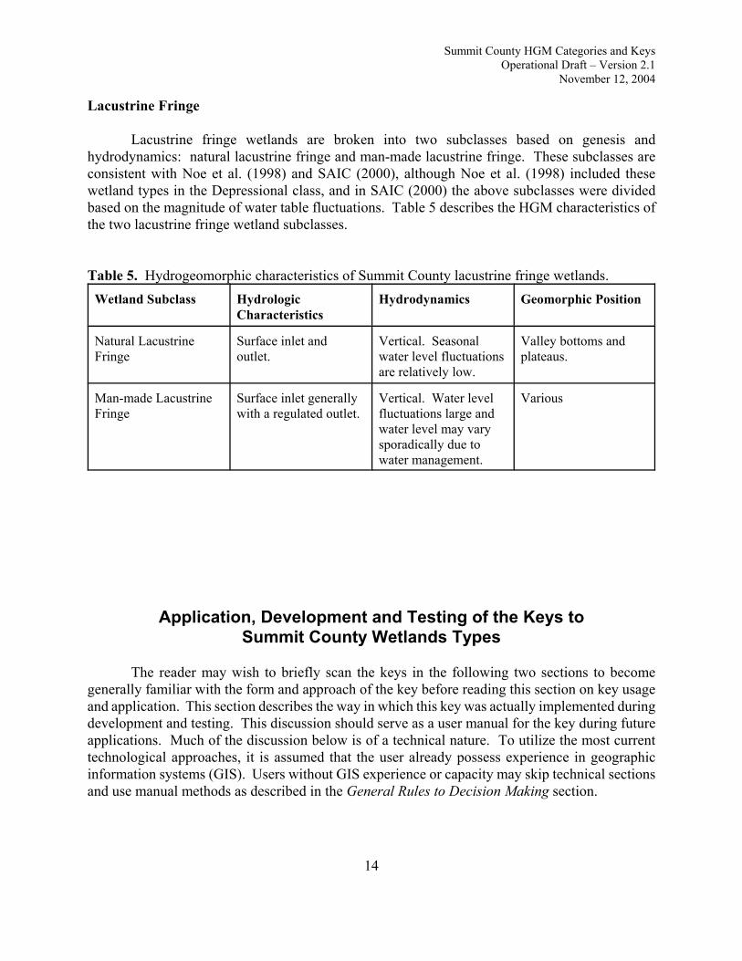
Summit County HGM Categories and KeysOperational Draft – Version 2.1
November 12, 2004
14
Lacustrine Fringe
Lacustrine fringe wetlands are broken into two subclasses based on genesis andhydrodynamics: natural lacustrine fringe and man-made lacustrine fringe. These subclasses areconsistent with Noe et al. (1998) and SAIC (2000), although Noe et al. (1998) included thesewetland types in the Depressional class, and in SAIC (2000) the above subclasses were dividedbased on the magnitude of water table fluctuations. Table 5 describes the HGM characteristics ofthe two lacustrine fringe wetland subclasses.
Table 5. Hydrogeomorphic characteristics of Summit County lacustrine fringe wetlands.Wetland Subclass Hydrologic
CharacteristicsHydrodynamics Geomorphic Position
Natural LacustrineFringe
Surface inlet andoutlet.
Vertical. Seasonalwater level fluctuationsare relatively low.
Valley bottoms andplateaus.
Man-made LacustrineFringe
Surface inlet generallywith a regulated outlet.
Vertical. Water levelfluctuations large andwater level may varysporadically due towater management.
Various
Application, Development and Testing of the Keys toSummit County Wetlands Types
The reader may wish to briefly scan the keys in the following two sections to becomegenerally familiar with the form and approach of the key before reading this section on key usageand application. This section describes the way in which this key was actually implemented duringdevelopment and testing. This discussion should serve as a user manual for the key during futureapplications. Much of the discussion below is of a technical nature. To utilize the most currenttechnological approaches, it is assumed that the user already possess experience in geographicinformation systems (GIS). Users without GIS experience or capacity may skip technical sectionsand use manual methods as described in the General Rules to Decision Making section.

Summit County HGM Categories and KeysOperational Draft – Version 2.1
November 12, 2004
1 Web site addresses (URLs) are current as of time of publishing, but are subject tochange.
15
GIS Development
A GIS was developed using ArcView version 8.1 software (ESRI 2001). Data incorporatedinto the GIS came from a variety of sources. All GIS data was projected into the UniversalTransverse Mercator (UTM) system using the North American Datum of 1927 (NAD 27). DigitalUSGS 7.5 minute quadrangles in GeoTIFF format comprised the base layer. GeoTIFFs are availablefrom the Natural Resources Conservation Service’s (NRCS) Geospatial Data Gateway1
(http://www.lighthouse.nrcs.usda.gov/gateway/gatewayhome.html); although the GeoTIFFs usedin this project were obtained from a commercial source.
Wetland polygons were obtained from three aerial photograph surveys of Summit County.Data were provided by Summit County. Each aerial photograph data source is described in SAIC(2002). The original wetland classifications were converted by SAIC (2000 and 2002) tohydrogeomorphic categories based on reinterpretation of aerial photographs, topographical data, andfield surveys.
A 10 meter DEM was used to derive 6 m (20 ft.) topographical contours. Wetlandtopographic gradient was determined by defining an axis within the widest or longest portion of thewetland perpendicular to its topographical gradient. The length or width of the wetland along thisaxis was then measured using the ArcView “Measure” tool. Finally, the change in elevation acrossthe wetland was determined by counting contour lines and multiplying by the contour interval.When a wetland began or ended between contours, elevation was estimated based on the relativeproportion of the contour interval covered by the wetland.
Stream ordering was carried out by hand using Strahler’s (1952) method. Ordering wasapplied to 1:100,000 digital line graphics (DLGs) and was completed by Summit CountyGovernment. A field containing stream order data was added to the stream digital line graphic(DLG) attribute table.
Geologic data for the county were obtained from the Denver and Leadville 1 X 2°(1:250,000) Geologic Quadrangles. These data files are available through the USGS web page ath t t p : / / g r e e n w o o d . c r . u s g s . g o v / p u b / m f - m a p s / m f - 2 3 4 7 a n dhttp://greenwood.cr.usgs.gov/pub/open-file-reports/ofr-99-0427, respectively.
Soil data were derived from two sources. Soil Survey Geographic Database (SSURGO) datawere used were available. These data are the most detailed digital soil data available in the state,but coverage of Summit County is incomplete. SSURGO data are available at:http://www.ftw.nrcs.usda.gov/ssurgo/metadata/co690.html. Where SSURGO data were unavailable,coarser State Soil Geographic Database (STATSGO) data were used. These data, compiled at ascale of 1:250,000, are available at: http://www.ftw.nrcs.usda.gov/stat_data.html.

Summit County HGM Categories and KeysOperational Draft – Version 2.1
November 12, 2004
16
Figure 1. Separation of wetland types based on the relativecontribution of hydrologic inputs. From Brinson (1993)
General Rules to Decision Making
Determination of many hydrogeomorphic traits, such as gradient or stream order, is straightforward using GIS or even simple paper 7.5' topographical quadrangles. Other characteristics suchas local soil composition or dominant hydrologic inputs may be more difficult to determine due tolack of site specific data or resolution limitations. What follows are some general guidelines towetland characterization in cases where description may not be clear cut or where data limitationsexist.
Most wetlands have somewhat mixed hydrologies. Of course all wetlands receive meteoricinputs, but most also receive varying degrees of surface and/or groundwater inputs. Brinson (1993),for example, provided a triangular ordination of wetland type based on the relative contribution ofprecipitation, groundwater and surface water inputs to the total wetland water budget (Fig. 1).
For this HGM classification, in all cases, wetlands should be grouped into classes based onthe dominant hydrologic source or process. Considering only ground and surface water inputs,riverine wetlands should receive more than 50 % of their hydrologic input from surface water,whereas slope wetlands should derive more than 50% of their hydrologic input from groundwater.As detailed in the description of Summit County wetland subclasses above, water sources ofdepressional and lacustrine fringe wetlands can vary.

Summit County HGM Categories and KeysOperational Draft – Version 2.1
November 12, 2004
17
In practical terms, separating riverine from slope wetlands is commonly quite difficult and,often arbitrary since these two types of systems may be interdependent and spatially intermixed.If fine scale detail is required for a particular application, large contiguous wetlands containing amix of wetland subclasses can be broken in multiple polygons (Partial Wetland Assessment Areassensu Smith et al. 1996). For larger-scale studies this level of subdivision may not be valuable.
If a data source is lacking or its resolution is insufficient, secondary indicators may provideadequate evidence for decision making and classification. If some wetland characteristics can notbe determined, the wetland can be left partially classified. For example a slope wetland could behydrogeomorphically classified as “isolated, low gradient” even if soil composition is unknown.Examples of common hydrologic, geologic and edaphic indicators are provided below to helpresolve common ambiguous situations that could arise while using these keys.
Indicators of Hydrology in Riverine, Slope and Lacustrine Fringe WetlandsSeparating riverine from slope wetlands is the greatest challenge in this method, since the
two types are often adjacent to one another, or form portions of a greater wetland complex. Slopewetlands at the base of stream terraces – both large and small – and flow-through slope wetlands arethe hardest to distinguish and separate from riverine wetlands. In fact, these wetlands may be soclosely associated that their separation is somewhat artificial. Therefore, while a greater number orerrors may in classifying these wetlands the consequences of doing so should generally be low. Aswritten before, in classifying a wetland based on hydrology, the dominant hydrologic input shouldbe used to determine wetland class. If different water sources dominate distinctly different portionsof a wetland, that wetland should be subdivided to reflect the situation. The followingcharacteristics help to distinguish hydrologic types when specific hydrologic data is not available.
C Flow-through slope wetlands can often be identified based on the following characteristics:The stream channel is low order (1st to 3rd) and wetland areas extend up adjacent valleyslopes, well above the channel elevation. This characteristic shows that wetlands receivewater from sources other than the alluvial system. Presence of a flow-through slope wetlandmay also be indicated by asymmetry of the wetland with respect to the channel. That is,within a symmetric channel valley, the wetland will be relatively broad and/or wide on theside of the channel possessing the slope wetland. The wetland on the opposite channel, willbe more narrow due to the absence of non-alluvial, groundwater input (See Appendix 1).
C Presence of a slope wetland is often indicated by the existence of a wetland on a slope or ata slope break with no other apparent source of water. Ponds may or may not be present. Ifa pond is present, the wetland may require division into slope and a depressional portions.
C Slope wetlands often occur at the base of riparian terraces, where an abrupt change in slopecauses groundwater to emerge. Slope wetlands that occur under these circumstances mayoften be distinguished from adjacent riverine wetlands in their spatial separation from thechannel and origination at the base of terraces. They may also extend up the terrace slope

Summit County HGM Categories and KeysOperational Draft – Version 2.1
November 12, 2004
18
well above the alluvial aquifer, they may be physically separated from other riverinewetlands in the floodplain, and they may develop outlet channels which flow into the mainriver or stream channel.
C Slope wetlands are often found on or near the shores of reservoirs or natural lakes. In thecase of reservoirs, historically expansive slope wetland complexes have frequently beenartificially flooded, and remnants of the wetlands exist on the lake fringe. If groundwaterinputs, rather than lake water levels, still dominate a wetland’s hydrology, the wetlandshould be classified as slope. An indication of this condition is when the wetland extendswell above the elevation of the lake’s surface.
Indicators of Soil Composition in Slope Wetlands
C Below 8500' a.m.s.l. it is highly unlikely that a slope wetland would possess organic soils.
C It is uncommon for very steep slope wetlands to possess organic soils.
Indicators of Geologic Composition in Depressional WetlandsC Large-scale hummocky terrain and/or clustering of small, somewhat-circular depressional
wetlands is usually indicative of glacial moraines and outwash. Therefore, depressionalwetlands located in such areas should be classified as kettle ponds unless additionalcontradictory evidence exists.
Testing and Evaluation of the HGM Wetland Key
General ApproachThe HGM categories devised in this classification were based on pre-existing literature,
consultation with local experts and professional judgement, as explained in the Introduction sectionof this document. The hierarchical dichotomous key algorithm was produced based distinguishingbetween the primary attributes defining a wetland category (either class or subclass). Subsequentto testing, this algorithm was revised to increase clarity and usability.
Quality assurance/control (QA/QC) documentation generally considers several proceduralattributes including: 1) accuracy; 2) precision; 3) completeness; and 4) representativeness (US EPA,1995). Other common QA/QC parameters were not applicable to this project since it did not containlaboratory analyses and no comparisons to other data sets were made. Determination ofmethodological accuracy, completeness and representativeness are described below. A measure ofmethod precision such as relative standard deviation or percent difference could not be used here

Summit County HGM Categories and KeysOperational Draft – Version 2.1
November 12, 2004
19
since all analyses were completed by a single individual and repeated classification of polygons(“repeated measure”) would be strongly biased by the classifier’s experience.
The wetland data set, assembled by SAIC for Summit County as described in theIntroduction section, was used to test the accuracy of the classification key. Wetland classes andsubclasses assigned to each wetland polygon in this data set were essentially taken as “true” values.The exception to this was when errors in stream ordering were encountered in the Summit Countydata set. Stream order calculation, which defines riverine wetland subclass, was performed “on-the-fly” during the Summit County wetland data set construction. For keying, an updated GIS layercontaining a Digital Line Graphic showing stream order was used. When inconsistencies arosebetween the data sets, stream order would be manually re-evaluated. In every case, the GIS DLGof stream order was correct.
One hundred randomly chosen wetland polygons were selected from the Summit County dataset. Each randomly selected wetland polygon was first keyed to class and then subclass using thisclassification algorithm and the GIS resources described in the Introduction section. Uponcompletion of keying, the wetland category obtained using this algorithm was compared to thatcontained in the SAIC data set. To assess the accuracy of this key three conditions were defined:1) correct class and subclass designation; 2) correct class and incorrect subclass designation; 3)incorrect class and subclass designation. The distribution of wetlands in each of these threecategories was used to determine the accuracy of the key.
Percent completeness was calculated as: %C = (v/T)*100, where v = the total number ofvalid observations and T = the total number of observations (US EPA 1995). Representativenesswas insured by using a random sampling approach and using a sample size large enough such thatall wetland classes were sampled. Due to the strong disparities in the commonness of the variouswetland types, coupled with the random sampling regime, the sample size of each wetland classdiffered.
Key Testing ResultsThe wetland class distribution of the 100 randomly selected wetland polygons is provided
in the table below. Of the 100 polygons, 13 could not be used for comparative testing since theywere left unclassified in the Summit County data set. Thus sampling completeness was 87%.
HGM Class Number represented insample
Depression 7
Lacustrine Fringe 2
Riverine 52
Slope 26
Unclassified 13
Total 100

Summit County HGM Categories and KeysOperational Draft – Version 2.1
November 12, 2004
20
There was a remarkable correspondence between the wetland types as designated in theSummit County data set and the wetlands classified using this keying algorithm; that is, the key wasshown to be highly accurate. Eighty-three of 87 wetlands (95%) were classified into the correctwetland class, while 79 of 87 wetlands (91%) were correctly classified to subclass. Only about 5%of wetlands were miss-classified at the class level. Classification errors were of three types: 1)Slope classified as riverine; 2) Slope classified as lacustrine fringe; and 3) Riverine classified asslope.
In the first case, flow-through, slope wetlands were classified as riverine due to their similarappearances and landscape settings. In the second case, slope wetlands were classified as lacustrinefringe when former slope wetland complexes were partially flooded by reservoir waters, andmarginal portions of the wetland remained beyond the reservoir shores. Lastly, one riverine wetlandwas classified as slope. In this case the wetland occurred in the floodplain near a terrace base, whichis a common landscape position for slope wetlands. “Decision rules” to help determine wetland typewere generated to mitigate errors in cases such as these. These rules are provided above in theGeneral Rules to Decision Making section.

Summit County HGM Categories and KeysOperational Draft – Version 2.1
November 12, 2004
21
KEYS TO SUMMIT COUNTY WETLANDCLASSES AND SUBCLASSES
Following the keys are illustrative examples of wetland types depicted in a GIS

Summit County HGM Categories and KeysOperational Draft – Version 2.1
November 12, 2004
22
KEY TO WETLAND CLASSES PRESENT IN SUMMITCOUNTY, COLORADO
1a. Wetland is found on the margin of a natural lake or reservoir larger than 0.5 ha with waterdepth exceeding 2 m, or wetland is located on the margin of an island . . . . . . . . . . . . . . .. . . . . . . . . . . . . . . . . . . . . . . . . . . . . . . . . . . . . . . . . . . . LACUSTRINE FRINGE WETLAND
1b. Wetland is not associated with a natural lake or reservoir . . . . . . . . . . . . . . . . . . . . . . . . 2
2a. Wetland surrounds and includes a shallow, open water area. Wetland is not located in anactive alluvial floodplain, nor is it a beaver pond (these wetlands are classified as Riverine).Wetland is located in an area of closed contour topography and may be hydrologicallyisolated, have a surface inlet, have a surface outlet, or be a through-flow system (inlet andoutlet present). Surface water inflow and outflow may be strongly seasonal . . . . . . . . . .. . . . . . . . . . . . . . . . . . . . . . . . . . . . . . . . . . . . . . . . . . . . . . . . . DEPRESSIONAL WETLAND
2b. Wetland possesses open-contour topography, with or without surface water inlets or outlets. . . . . . . . . . . . . . . . . . . . . . . . . . . . . . . . . . . . . . . . . . . . . . . . . . . . . . . . . . . . . . . . . . . . . . 3
3a. Wetland is within the 100-year floodplain of a perennial stream or river and not located atthe base of a fluvial terrace . . . . . . . . . . . . . . . . . . . . . . . . . . . . . . . RIVERINE WETLAND
3b. Wetland is not located within the 100-year floodplain of a perennial stream, or if it is withinthe 100-year floodplain, wetland is located at the base of a fluvial terrace. Groundwaterdischarge dominates hydrologic inputs. Wetland may be on sloping or relatively flat terrain(1 % gradient). Springs or seeps are usually present . . . . . . . . . . . . . . SLOPE WETLAND

Summit County HGM Categories and KeysOperational Draft – Version 2.1
November 12, 2004
23
KEY TO WETLAND SUBCLASSES PRESENT IN SUMMITCOUNTY, COLORADO
KEY TO LACUSTRINE FRINGE WETLAND SUBCLASSES
1a. Wetland is located on the shore of a natural lake. Wetland hydrology is directly controlledby lake water levels. Water level is relatively stable with small, seasonal variations . . . .. . . . . . . . . . . . . . . . . . . . . . . . . . . . . . . . . . . . . . . . . Natural lacustrine fringe wetlands
1b. Wetland is located on the shore of a man-made lake or reservoir. Wetland hydrology isdirectly controlled by lake water levels. Lake water level commonly experiences largefluctuations in water level seasonally, or sporadically through active water management .. . . . . . . . . . . . . . . . . . . . . . . . . . . . . . . . . . . . . . Man-made lacustrine fringe wetlands
KEY TO DEPRESSIONAL WETLAND SUBCLASSES
1a. Wetland includes an open-water kettle pond formed during Quaternary glacial retreat. Kettleponds and associated wetlands are often roughly circular in shape and are associated withglacial till. The kettle pond wetland may include areas of open-water, floating vegetationmats, or solid organic or mineral soils. . . . . . . . . . . . . . . . . . . . . . . Kettle pond wetland
1b. Wetland not as above . . . . . . . . . . . . . . . . . . . . . . . . . . . . . . . . . . . . . . . . . . . . . . . . . . . . . 2
2a. Wetland located in a relic river oxbow or meander scar and is located on a geomorphicsurface above the active floodplain, or wetland has been isolated from the active floodplainthrough the effects of anthropogenic structures such as dams or dikes. Isolated riverinedepressional wetlands may receive hydrologic inputs through precipitation, groundwaterinflow and surface runoff . . . . . . . . . . . . . . . . . . Isolated riverine depressional wetland
2b. Wetland is in a geomorphic position not described above. Wetland may be man-made suchas a cattle pond, or natural such as a snowmelt-fed wetland above tree line . . . . 3
3a. Wetland was formed by natural processes. These wetlands may be located in a variety ofhydrogeomorphic situations, such as in snowmelt-fed depressions above tree line or behinddammed landslide scars . . . . . . . . . . . . . . . . . . . . Other natural depressional wetlands
3b. Wetland is man-made. These wetlands can be found in virtually any hydrogeomorphicposition and may be hydrologically maintained solely through artificial means . . . . . . . . . . . . . . . . . . . . . . . . . . . . . . . . . . . . . . . . . . . . . . . . . . Man-made depressional wetlands

Summit County HGM Categories and KeysOperational Draft – Version 2.1
November 12, 2004
24
KEY TO RIVERINE WETLAND SUBCLASSES
1a. Wetland and associated stream possess a high gradient (greater than approximately 8 %), orwetland and floodplain tightly bounded by geomorphological features such as narrow valleywalls or cliff scarps. Due to the steep gradient and/or floodplain confinement, thesewetlands will typically be narrow and closely associated with the active channel . . . . . . 2
1b. Wetland and associated stream possess a moderate to low gradient (between 0 and ~ 8%),and wetland and floodplain broadly bounded by geomorphological features such as terracesor cliff scarps. Relatively low gradients and broad floodplains allow the development ofmore expansive riverine wetlands . . . . . . . . . . . . . . . . . . . . . . . . . . . . . . . . . . . . . . . . . . . 4
2a. Wetland is located on a stream with an order between 1 and 3 . . . . . . . . . . . . . . . . . . . . . .. . . . . . . . . . . . . . . . . . . . . . . Low-order, high-gradient or bounded, riverine wetland
2b. Wetland is located on a higher order stream . . . . . . . . . . . . . . . . . . . . . . . . . . . . . . . . . . . 3
3a. Wetland is located on a stream with an order between 4 and 5 . . . . . . . . . . . . . . . . . . . . . .. . . . . . . . . . . . . . . . . . . . . . . Mid-order, high-gradient or bounded, riverine wetland
3b. Wetland is located on a stream with an order between 6 and 7 . . . . . . . . . . . . . . . . . . . . . .. . . . . . . . . . . . . . . . . . . . . . . High-order, high-gradient or bounded riverine wetland
4a. Wetland is located on a stream with an order between 1 and 3 . . . . . . . . . . . . . . . . . . . . . .. . . . . . . . . . . . . . . . . . . . . . . . Low-order, low-gradient, unbounded riverine wetland
4b. Wetland is located on a higher order stream . . . . . . . . . . . . . . . . . . . . . . . . . . . . . . . . . . . 3
5a. Wetland is located on a stream with an order between 4 and 5 . . . . . . . . . . . . . . . . . . . . . .. . . . . . . . . . . . . . . . . . . . . . . . Mid-order, low-gradient, unbounded, riverine wetland
5b. Wetland is located on a stream with an order between 6 and 7 . . . . . . . . . . . . . . . . . . . . . .. . . . . . . . . . . . . . . . . . . . . . . . High-order, low-gradient, unbounded riverine wetland

Summit County HGM Categories and KeysOperational Draft – Version 2.1
November 12, 2004
25
KEY TO SLOPE WETLAND SUBCLASSES
1a. No apparent surface inflow from a stream or other water body, and no apparent outflow toa stream or water body . . . . . . . . . . . . . . . . . . . . . . . . . . Isolated slope wetlands sub-key
1b. Wetland possess an inlet channel, an outlet channel, or both . . . . . . . . . . . . . . . . . . . . . . 2
2a. Wetland possess both and inlet and an outlet channel . . . . . . . . . . . . . . . . . . . . . . . . . . . .. . . . . . . . . . . . . . . . . . . . . . . . . . . . . . . . . . . . . . . Through-flow slope wetlands sub-key
2b. Wetland posses only an inlet or and outlet channel . . . . . . . . . . . . . . . . . . . . . . . . . . . . . 3
3a. Wetland only has an inlet channel. Channelized flow become disperse and eventually ceaseswithin the wetland . . . . . . . . . . . . . . . . . . . . . . . . . . . . . . Inflow slope wetlands sub-key
3b. Wetland only has an outlet channel. Wetland forms a stream headwaters . . . . . . . . . . . . .. . . . . . . . . . . . . . . . . . . . . . . . . . . . . . . . . . . . . . . . . . . Outflow slope wetlands sub-key
Slope Wetland Sub-keys
Isolated Slope Wetland Sub-key1a. Wetland topographical gradient between 0 - 4 % . . . . . . . . . . . . . . . . . . . .
. . . . . . . . . . . . . . . . . . . . . . . . . Isolated, shallow gradient, slope wetland
i. Wetland only having mineral soils . . . . . . . . . . . . . . . . . . . . . . . . .. . . . . . . Isolated, shallow-gradient, mineral soil slope wetland
ii. Wetland possesses organic soils . . . . . . . . . . . . . . . . . . . . . . . . . . .. . . . . . . Isolated, shallow-gradient, organic soil slope wetland
1b. Wetland topographical gradient > 4% . . . . . . . . . . . . . . . . . . . . . . . . . . . . 2
2a. Wetland topographical gradient > 4 % to 10 % . . . . . . . . . . . . . . . . . . . . . .. . . . . . . . . . . . . . . . . . . . . . . . Isolated, moderate-gradient slope wetlands
i. Wetland only having mineral soils . . . . . . . . . . . . . . . . . . . . . . . . .. . . . . . Isolated, moderate-gradient, mineral soil slope wetland

Summit County HGM Categories and KeysOperational Draft – Version 2.1
November 12, 2004
26
ii. Wetland possesses organic soils . . . . . . . . . . . . . . . . . . . . . . . . . . .. . . . . . Isolated, moderate-gradient, organic soil slope wetland
2b. Wetland topographical gradient > 10% . . . . . . . . . . . . . . . . . . . . . . . . . . . .. . . . . . . . . . . . . . . . . . . . . . . . . . . . Isolated, high gradient slope wetlands
iii. Wetland only having mineral soils . . . . . . . . . . . . . . . . . . . . . . . . .. . . . . . . . . . Isolated, high-gradient, mineral soil slope wetland
ii. Wetland possesses organic soils . . . . . . . . . . . . . . . . . . . . . . . . . . .. . . . . . . . . . Isolated, high-gradient, organic soil slope wetland
Through-flow Slope Wetland Sub-key1a. Wetland topographical gradient between 0 - 4 % . . . . . . . . . . . . . . . . . . . .
. . . . . . . . . . . . . . . . . . . . . Through-flow, shallow gradient, slope wetland
i. Wetland only having mineral soils . . . . . . . . . . . . . . . . . . . . . . . . .. . Through-flow, shallow-gradient, mineral soil slope wetland
ii. Wetland possesses organic soils . . . . . . . . . . . . . . . . . . . . . . . . . . .. . Through-flow, shallow-gradient, organic soil slope wetland
1b. Wetland topographical gradient > 4% . . . . . . . . . . . . . . . . . . . . . . . . . . . . 2
2a. Wetland topographical gradient > 4 % to 10 % . . . . . . . . . . . . . . . . . . . . . .. . . . . . . . . . . . . . . . . . . Through-flow, moderate-gradient slope wetlands
i. Wetland only having mineral soils . . . . . . . . . . . . . . . . . . . . . . . . .Through-flow, moderate-gradient, mineral soil slope wetland
ii. Wetland possesses organic soils . . . . . . . . . . . . . . . . . . . . . . . . . . .. Through-flow, moderate-gradient, organic soil slope wetland
2b. Wetland topographical gradient > 10% . . . . . . . . . . . . . . . . . . . . . . . . . . . .. . . . . . . . . . . . . . . . . . . . . . . Through-flow, high-gradient slope wetlands
iii. Wetland only having mineral soils . . . . . . . . . . . . . . . . . . . . . . . . .. . . . . Through-flow, high-gradient, mineral soil slope wetland
ii. Wetland possesses organic soils . . . . . . . . . . . . . . . . . . . . . . . . . . .. . . . . Through-flow, high-gradient, organic soil slope wetland
Inflow Slope Wetland Sub-key1a. Wetland topographical gradient between 0 - 4 % . . . . . . . . . . . . . . . . . . . .
. . . . . . . . . . . . . . . . . . . . . . . . . . . Inflow, shallow gradient, slope wetland
i. Wetland only having mineral soils . . . . . . . . . . . . . . . . . . . . . . . . .. . . . . . . . Inflow, shallow-gradient, mineral soil slope wetland
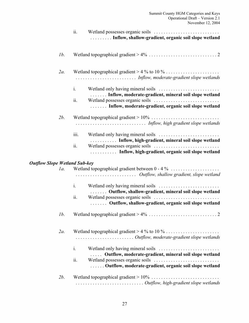
Summit County HGM Categories and KeysOperational Draft – Version 2.1
November 12, 2004
27
ii. Wetland possesses organic soils . . . . . . . . . . . . . . . . . . . . . . . . . . .. . . . . . . . . Inflow, shallow-gradient, organic soil slope wetland
1b. Wetland topographical gradient > 4% . . . . . . . . . . . . . . . . . . . . . . . . . . . . 2
2a. Wetland topographical gradient > 4 % to 10 % . . . . . . . . . . . . . . . . . . . . . .. . . . . . . . . . . . . . . . . . . . . . . . . Inflow, moderate-gradient slope wetlands
i. Wetland only having mineral soils . . . . . . . . . . . . . . . . . . . . . . . . .. . . . . . . Inflow, moderate-gradient, mineral soil slope wetland
ii. Wetland possesses organic soils . . . . . . . . . . . . . . . . . . . . . . . . . . .. . . . . . . Inflow, moderate-gradient, organic soil slope wetland
2b. Wetland topographical gradient > 10% . . . . . . . . . . . . . . . . . . . . . . . . . . . .. . . . . . . . . . . . . . . . . . . . . . . . . . . . . Inflow, high gradient slope wetlands
iii. Wetland only having mineral soils . . . . . . . . . . . . . . . . . . . . . . . . .. . . . . . . . . . . Inflow, high-gradient, mineral soil slope wetland
ii. Wetland possesses organic soils . . . . . . . . . . . . . . . . . . . . . . . . . . .. . . . . . . . . . . Inflow, high-gradient, organic soil slope wetland
Outflow Slope Wetland Sub-key1a. Wetland topographical gradient between 0 - 4 % . . . . . . . . . . . . . . . . . . . .
. . . . . . . . . . . . . . . . . . . . . . . . . Outflow, shallow gradient, slope wetland
i. Wetland only having mineral soils . . . . . . . . . . . . . . . . . . . . . . . . .. . . . . . . Outflow, shallow-gradient, mineral soil slope wetland
ii. Wetland possesses organic soils . . . . . . . . . . . . . . . . . . . . . . . . . . .. . . . . . . Outflow, shallow-gradient, organic soil slope wetland
1b. Wetland topographical gradient > 4% . . . . . . . . . . . . . . . . . . . . . . . . . . . . 2
2a. Wetland topographical gradient > 4 % to 10 % . . . . . . . . . . . . . . . . . . . . . .. . . . . . . . . . . . . . . . . . . . . . . . Outflow, moderate-gradient slope wetlands
i. Wetland only having mineral soils . . . . . . . . . . . . . . . . . . . . . . . . .. . . . . Outflow, moderate-gradient, mineral soil slope wetland
ii. Wetland possesses organic soils . . . . . . . . . . . . . . . . . . . . . . . . . . .. . . . . . Outflow, moderate-gradient, organic soil slope wetland
2b. Wetland topographical gradient > 10% . . . . . . . . . . . . . . . . . . . . . . . . . . . .. . . . . . . . . . . . . . . . . . . . . . . . . . . . Outflow, high-gradient slope wetlands

Summit County HGM Categories and KeysOperational Draft – Version 2.1
November 12, 2004
28
iii. Wetland only having mineral soils . . . . . . . . . . . . . . . . . . . . . . . . .. . . . . . . . . . Outflow, high-gradient, mineral soil slope wetland
ii. Wetland possesses organic soils . . . . . . . . . . . . . . . . . . . . . . . . . . .. . . . . . . . . . Outflow, high-gradient, organic soil slope wetland

Summit County HGM Categories and KeysOperational Draft – Version 2.1
November 12, 2004
3 Modified from Bisson and Montgomery (1996)4 Modified from Smith et al. (1995).
29
Confined Reaches Unconfined Reaches
Glossary
Confined (tightly-bounded) or Unconfined (loosely-bounded) Floodplain3: The confinedfloodplain is one in which the hillslopes narrowly constrain the valley floor with little or nofloodplain development. An unconfined floodplain is one in which valley hillslopes only broadlyconstrain channel movement and floodplain development. Unconfined floodplains are often, butnot always associated with broad riparian zones. A gauge of confinement is as follows:
Valley floor width < 3 channel widths wide S t r o n g l y t o s o m e w h a tconfined
Valley floor width > 3 channel widths wide S o m e w h a t c o n f i n e d t ounconfined
Depressional Wetland:4 Depressional wetlands are found within topographic depressionspossessing closed elevational contours that allow the accumulation of surface water.
Hydrogeomorphic Approach: An approach to wetland classification which categorizes wetlandsbased on commonalities in their geomorphology, hydrology and hydrodynamics.
Lacustrine Fringe Wetland:4 A wetland type found adjacent to lakes where the water elevation ofthe lake maintains the water table in the wetland. Lacustrine fringe wetlands may also be found onislands within lakes.

Summit County HGM Categories and KeysOperational Draft – Version 2.1
November 12, 2004
30
Organic soils: Organic soils are those soils which meet the NRCS (1998) definition of a Histosolwhich is provided below.
Histosols:Do not have andic soil properties in 60 percent or more of the thickness between the soil surface and either a depth of60 cm or a densic, lithic, or paralithic contact or duripanif shallower; and 2. Have organic soil materials that meet one or more of the following:a. Overlie cindery, fragmental, or pumiceous materials and/or fill their interstices1 and directly below these materials,have a densic, lithic, or paralithic contact;orb. When added with the underlying cindery, fragmental, or pumiceous materials, total 40 cm or more between the soilsurface and a depth of 50 cm; orc. Constitute two-thirds or more of the total thickness of the soil to a densic, lithic, or paralithic contact and have nomineral horizons or have mineral horizons with a total thickness of 10 cm or less; ord. Are saturated with water for 30 days or more per year in normal years (or are artificially drained), have an upperboundary within 40 cm of the soil surface, and have a total thickness of either:(1) 60 cm or more if three-fourths or more of theirvolume consists of moss fibers or if their bulk density,moist, is less than 0.1 g/cm3; or(2) 40 cm or more if they consist either of sapric orhemic materials, or of fibric materials with less thanthree-fourths (by volume) moss fibers and a bulkdensity, moist, of 0.1 g/cm3 or more.
Riverine Wetland:4 A wetland that occurs within a floodplain or riparian corridor. The dominantwater source for this type of wetland is overbank flow from the channel or subsurface hydrologicconnection to the alluvial aquifer.
Slope Wetland:4 A wetland whose hydrology is dominated by groundwater discharge. Slopewetlands lack significant depressional water storage due to their lack of closed contours. Slopewetlands may occur on nearly flat landscapes.
Stream order: A means of classifying streams according to their importance within the drainagebasin. The lowest order streams are the most minor tributaries. This study used the Strahler (1952)stream ordering method.
Hydrogeomorphic Wetland Class:4 The highest level in the hydrogeomorphic (HGM) wetlandclassification. This document includes four HGM classes: Slope, Riverine, Depression, andLacustrine Fringe. Class are based on gross difference site hydrology, geomorphology andhydrodynamics.
Hydrogeomorphic Wetland Subclass:4 Wetlands within a region that are similar based onhydrogeomorphic classification factors. There are multiple subclasses within each wetland class.The actual number of wetland subclasses defined is based on the known diversity of wetlands withina class and particular assessment objectives.
Alluvial: Structures and features produced through river-induced deposition.

Summit County HGM Categories and KeysOperational Draft – Version 2.1
November 12, 2004
31
Fluvial: Structures, features and characteristics produced through stream action.
Scarp: A steep slope or cliff connecting the surface of a former floodplain to a lower surface.

Summit County HGM Categories and KeysOperational Draft – Version 2.1
November 12, 2004
32
REFERENCES CITED
Adamus, P. R. 2001. Guidebook for hydrogeomorphic (HGM)-based assessment of Oregon wetlandand riparian sites: Statewide classification and profiles. Oregon Division of State Lands,Salem, Or .
Bisson, P. and D. Montgomery. 1996. Valley segments, stream reaches, and channel units. In:Hauer, F. R. and G. Lamberti (eds.), Methods of Stream Ecology. Academic Press, NewYork.
Brinson, M. M. 1993. A hydrogeomorphic classification for wetlands. Technical Report WRP-DE-4, U.S. Army Engineer Waterways Experiment Station, Vicksburg, MS .
Cowardin, L. M. Carter, V. Golet, F. C. and LaRoe, E. T. 1979. Classification of wetlands anddeepwater habitats of the United States. U.S. Fish and Wildlife Service, Biological ServicesProgram. Report No. FWS/OBS-79/31 .
Gwin, S. Kentula, M. and Shaffer, P. 1999. Evaluating the effects of wetland regulation throughhydrogeomorphic classification and landscape profiles. Wetlands 19: 477-489.
Hauer, F. R. and Smith, R. D. 1998. The hydrogeomorphic approach to functional assessment ofriparian wetlands: evaluating impacts and mitigation on river floodplains in the U.S.A.Freshwater Biology 40: 517-530.
Johnson, J. B. 2000. Documentation of reference conditions in the slope wetlands of the southernRocky Mountains: reference database, site descriptions, and revised functional models.Report Submitted to U.S. EPA , Region 8 and the Colorado Department of NaturalResources .
Keate, N. 1998. Utah Riverine Model: low gradient, low elevation, riverine wetlands of theColorado Plateau and Great Basin of Utah – Draft. Report submitted to U.S. EPA, Region8.
Keate, N. 2001. Utah montane slope (fens and wet meadows) functional assessment model (draft).Report submitted to U.S. EPA, Region 8 .
Noe, D. Cooper, D. Barry, A. Pavlik, M. Kolm, K. Harper-Arabie, R. Emerick, J. Arp, C. andChimner, R. 1998. Characterization and functional assessment of reference wetlands inColorado. Report submitted to Colorado Dept. of Natural Resources and US EPA RegionVIII .
SAIC. 2000. Summit County wetland functional assessment. Science Applications InternationalCorporation, Lakewood, CO. Report prepared for the Summit County CommunityDevelopment Division .

Summit County HGM Categories and KeysOperational Draft – Version 2.1
November 12, 2004
33
Smith, R. D. Ammann, A. Bartoldus, C. and Brinson, M. M. 1995. An approach for assessingwetland functions using hydrogeomorphic classification, reference wetlands and functionalindices. Technical Report WRP-DE-9, U.S. Army Corps of Engineer WaterwaysExperiment Station, Vicksburg, MS .
Strahler, A. N. 1957. Quantitative analysis of watershed geomorphology. AmericanGeophysical Union Transactions 38:1117-1142.
Tiner, R. 2000. Keys to waterbody type and hydrogeomorphic-type wetland descriptors for U.S.waters and wetlands (Operational Draft). U.S. Fish and Wildlife Service National WetlandsInventory Project Report, September 2000.
US EPA. 1995. Generic quality assurance project plan guidance for programs using communitylevel biological assessment in wadable streams and rivers. Office of Water, EPA 841-B-95-004.

Summit County HGM Categories and KeysOperational Draft – Version 2.1
November 12, 2004
34
APPENDIX 1
EXAMPLES OF KEYING WETLANDS USING TOPOGRAPHIC AND GIS DATA

Figure A1. A section of map showing the setting of a large, outflowslope wetland (lower left hand quarter of the map. The wetland,located in a alpine cirque, forms the headwaters of a stream systemflowing to the north. A similar, but smaller, wetland can be seen inthe lower right hand corner.
Figure A2. Map showing a isolated slope wetland occurring onthe slopes of Buffalo Mountain near tree line. In this case,groundwater that discharges in the alpine zone apparentlyrecharges as it flows onto the more shallowly graded subalpineslopes.

Figure A3. Four examples of through-flow slope wetlands. The asymmetrical shape andextension of the wetland well above the channel helps to identify these sites as slope, ratherthan, riverine wetlands.

Figure A4. Four low-order, narrow riverine wetlands (confined valley) oriented north-south
along the top of the figure. These streams are tributary to a mid-order (5 order) river with awell developed (unconfined) floodplain.
th
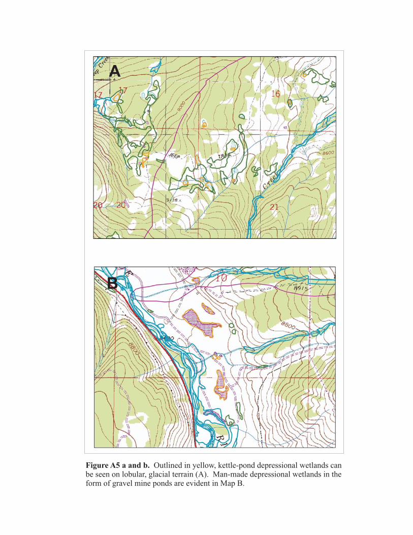
A
B
Figure A5 a and b. Outlined in yellow, kettle-pond depressional wetlands canbe seen on lobular, glacial terrain (A). Man-made depressional wetlands in theform of gravel mine ponds are evident in Map B.

Figure A6. Outlined in pale pink, man-made lacustrine fringe wetlands can be seen on themargins of Dillon Reservoir.