Hydraulics of Bridge Waterways

PDHengineer.com Course № C-8017

Hydraulics of Bridge Waterways

This document is the course text. You may review this material at your leisure before or after you purchase the course. If you have not already purchased the course, you may do so now by returning to the course overview page located at: http://www.pdhengineer.com/pages/C‐8017.htm (Please be sure to capitalize and use dash as shown above.) Once the course has been purchased, you can easily return to the course overview, course document and quiz from PDHengineer’s My Account menu. If you have any questions or concerns, remember you can contact us by using the Live Support Chat link located on any of our web pages, by email at [email protected] or by telephone toll‐free at 1‐877‐PDHengineer. Thank you for choosing PDHengineer.com.

© PDHengineer.com, a service mark of Decatur Professional Development, LLC. C‐8017 C1

Hydraulics of Bridge WaterwaysHDS 1

March 1978

Welcome toHDS1-Hydraulicsof BridgeWaterways.

Table of Contents

Preface

Forward

Author(s): Joseph N. Bradley, FHWA, Bridge Division

DISCLAIMER: During the editing of this manual for conversion to an electronicformat, the intent has been to keep the document text as close to the original aspossible. In the process of scanning and converting, some changes may havebeen made inadvertently.

http://aisweb/pdf2/library/Default.htm

Table of Contents for HDS 1-Hydraulics of Bridge Waterways

List of Figures List of Tables List of Equations

Cover Page : HDS 1-Hydraulics of Bridge Waterways

Chapter 1 : HDS 1 Introduction 1.1 General 1.2 Waterway Studies 1.3 Bridge Backwater 1.4 Nature of Bridge Backwater 1.5 Types of Flow Encountered 1.6 Field Verification 1.7 Definition of Symbols 1.8 Definition of Terms 1.9 Conveyance 1.10 Bridge Opening Ratio 1.11 Kinetic Energy Coefficient

Chapter 2 : HDS 1 Computation of Backwater 2.1 Expression of Backwater 2.2 Backwater Coefficient 2.3 Effect of M and Abutment Shape (Base Curves) 2.4 Effect of Piers (Normal Crossings) 2.5 Effects of Piers (Skewed Crossings) 2.6 Effect of Eccentricity 2.7 Effect of Skew

Chapter 3 : HDS 1 Difference in Water Level across Approach Embankments 3.1 Significance 3.2 Base Curves 3.3 Effects of Piers 3.4 Effect of Eccentricity 3.5 Drop in Water Surface Across Embankment (Normal Crossing) 3.6 Water Surface on Downstream Side of Embankment (Skewed Crossing)

Chapter 4 : HDS 1 Configuration of Backwater 4.1 Distance to Point of Maximum Backwater 4.2 Normal Crossings

4.3 Eccentric Crossings 4.4 Skewed Crossings

Chapter 5 : HDS 1 Dual Bridges 5.1 Arrangement 5.2 Backwater Determination 5.3 Drop in Water Surface Across Embankments

Chapter 6 : HDS 1 Abnormal Stage-Discharge Condition 6.1 Definition 6.2 Backwater Determination 6.3 Backwater Expression 6.4 Drop in Water Surface Across Embankments

Chapter 7 : HDS 1 Effect of Scour on Backwater 7.1 General 7.2 Nature of Scour 7.3 Backwater Determination 7.4 Enlarged Waterways

Chapter 8 : HDS 1 Superstructure Partially Inundated 8.1 The Problem 8.2 Upstream Girder in Flow (Case I) 8.3 All Girders in Contact with Flow (Case II) 8.4 Safety of Bridge 8.5 Flow over Roadway 8.6 Nottoway River Bridge

Chapter 9 : HDS 1 Spur Dikes 9.1 Introduction 9.2 Function and Geometry of Spur Dike 9.3 Length of Spur Dike 9.4 Other Considerations

Chapter 10 : HDS 1 Flow Passes Through Critical Depth (Type II) 10.1 Introduction 10.2 Backwater Coefficients 10.3 Recognition of Flow Type

Chapter 11 : HDS 1 Preliminary Field and Design Procedures 11.1 Evaluation of Flood Hazards 11.2 Site Study Outline 11.3 Hydrological Analysis Outline 11.4 Flood Magnitude and Frequency 11.5 Stage Discharge 11.6 Channel Roughness 11.7 Bridge Backwater Design Procedure

Chapter 12 : HDS 1 Illustrative Examples 12.1 Example 1: Normal Crossing Computation (1a)

Computation (1b)

Computation (1c)

Computation (1d)

Computation (1e)

Computation (1f)

Computation (1g)

12.2 Example 2: Dual Bridges Computation (2a)

Computation (2b)

Computation (2c)

12.3 Example 3: Skewed Crossing Computation (3a)

Computation (3b)

Computation (3c)

12.4 Example 4: Eccentric Crossing Computation (4a)

12.5 Example 5: Abnormal Stage-Discharge Computation (5a)

Computation (5b)

12.6 Example 6: Backwater with Scour Computation (6a)

Computation (6b)

Computation (6c)

Computation (6d)

12.7 Example 7: Upstream Bridge Girder in the Flow Computation (7a)

Computation (7b)

Computation (7c)

12.8 Example 8: Superstructure Partially Inundated Computation (8a)

Computation (8b)

12.9 Example 9: Flow Over Roadway Embankment 12.10 Example 10: Design of Spur Dike Computation (10a)

Computation (10b)

12.11 Example 11: Bridge Backwater with Supercritical Flow

Chapter 13 : HDS 1 Discussion of Procedures and Limitations of Method 13.1 Review of Design Methods 13.2 Further Research Recommended

Appendix A : HDS 1 Development of Expressions for Bridge Backwater A.1 Type I Flow (Subcritical) A.2 Type II Flow (Water Surface Passes Through Critical Depth) A.3 Type III Flow (Supercritical)

Appendix B: HDS 1 Basis of Revisions B.1 Backwater Coefficient Base Curves B.2 Distance to Maximum Backwater Curves B.3 Velocity Head Correction Factor, a2 B.4 Dual Bridges

Appendix C : HDS 1 Development of Chart for Determining Length of Spur Dikes

References

List of Figures for HDS 1-Hydraulics of Bridge Waterways

Back to Table of Contents

Figure 1. Flow lines for typical normal crossing.

Figure 2. Normal crossing: Wingwall abutments.

Figure 3. Normal crossings: Spillthrough abutments.

Figure 4. Types of flow encountered.

Figure 5. Aid for Estimating α2

Figure 6. Backwater coefficient base curves (subcritical flow).

Figure 7. Incremental backwater coefficient for piers.

Figure 8. Incremental backwater coefficient for eccentricity.

Figure 9. Skewed crossings.

Figure 10. Incremental backwater coefficient for skew.

Figure 11. Ratio of projected to normal length of bridge for equivalent backwater (skewed crossings).

Figure 12. Differential water level ratio base curves.

Figure 13. Distance to maximum backwater.

Figure 14. Backwater multiplication factor for dual bridges.

Figure 15. Differential level multiplication factor for dual parallel bridges.

Figure 16. Backwater with abnormal stage discharge condition.

Figure 17. Effect of scour on bridge backwater.

Figure 18. Scour at wingwall abutment and single circular piers (model).

Figure 19. Cross section of scour at upstream side of bridge (model).

Figure 20. Correction factor for backwater with scour.

Figure 21. Discharge coefficients for upstream girder in flow (case I).

Figure 22. Discharge coefficient for All girders in flow (case II).

Figure 23. Buoyant and horizontal forces moved these 80-foot spans downstream.

Figure 24. Discharge coefficients for flow over roadway embankments.

Figure 25. Missouri River Bridge on Route I-70.

Figure 26. Nottoway River Bridge on Virginia Route 40.

Figure 27. Flow concentration along upstream side of embankment at Big Nichols Creek.

Figure 28. Extent of scour measured After the flood at Big Nichols Creek.

Figure 29. Model of a spur dike.

Figure 30. Charts for determining length of spur dikes.

Figure 31. Spur dikes on model of Tarbela Bridge, Indus River, West Pakistan.

Figure 32. Spur dike on 45° skewed bridge Over Susquehanna River at Nanticoke Pa.

Figure 33. Plan and cross section of spur dike.

Figure 34. Tentative backwater coefficient curve for type II flow.

Figure 35. Status of U.S. Geological Survey nationwide flood frequency project.

Figure 36. Example 1: Plan and cross section of normal crossing.

Figure 37. Example 3: Plan for skewed crossing.

Figure 38. Examples 1-3: Conveyance and area at section 1.

Figure 39. Example 4: Cross section of eccentric river crossing.

Figure 40. Example 4: Stage-discharge curve for river at bridge site.

Figure 41. Example 4: Area and velocity-head coefficient.

Figure 42. Example 4: Conveyance at section 1.

Figure 43. Example 4: Composite backwater curves.

Figure 44. Example 4: Water surface at section 1.

Figure 45. Example 6: Backwater with Scour

Figure 46. Example 7, Example 8, and Example 9: Bridge backwater under less common conditions.

Figure 47. Example 11: Bridge backwater with supercritical flow.

Figure A-1. Flow types I, II, and III.

Figure A-2. Backwater coefficient curve for type I flow.

Figure A-3. Backwater coefficient curve for type II flow.

Figure B-1. Distance to Maximum backwater curves showing field data.

Figure B-2. Curve for determining velocity head coefficient, α2, showing field data.

Figure B-3. Differential level multiplication factor for dual parallel bridges.

Figure B-4. Backwater multiplication factor for dual parallel bridges.

Figure C-1. Length of spur dikes.


Chapter 1 : HDS 1Introduction

Go to Chapter 2

1.1 General

There was a time, now past, when backwater caused by the presence of bridges during floodperiods was considered a necessary nuisanceCfirst, because the public clamored for bridges toreplace ferries and fords; and second, because there was no accurate means of determining theamount of backwater a bridge would produce after it was in place. With the spread ofurbanization; with indefinite, unenforceable restrictions on the construction of housing andbusiness establishments on flood plains of rivers and streams throughout the country; with newhighway bridges being constructed at an ever-increasing rate; and with property valuesincreasing at an unprecedented rate in the past two decades, it is now imperative that thebackwater produced by new bridges be kept within very knowledgeable and reasonable limits.This places demands on the hydraulic engineer, who has not been consulted too often in thepast, to promote and develop a more scientific approach to the bridge waterway problem.Progress in structural design has kept pace with the times. Structural engineers are well awareof the economies which can be attained in the proper type, selection and design of a bridge of agiven overall length and height. The role of the hydraulic engineer in establishing what the lengthand vertical clearance should be and where the bridge should be placed is less well understooddue principally to the lack of hydrological and hydraulic information on the waterways.

In fact, until recently, bridge lengths and clearances have been proportioned principally on roughcalculations, individual judgment, and intuition. This may still be true in some cases. Today, traffic volumes have become so great on primary roads that bridge failures or bridges out ofservice for any length of time can cause severe economic loss and inconvenience; even closingone lane of an arterial highway for repairs creates pandemonium.

Confining flood waters unduly by bridges can cause excessive backwater resulting in flooding ofupstream property, backwater damage suits, overtopping of roadways, excessive scour underthe bridge, costly maintenance, or even loss of a bridge. On the other hand, over-design ormaking bridges longer than necessary for the sake of safety, can add materially to the initial cost,especially when dual or multiple lane bridges are involved. Both extremes in design have beenexperienced. Somewhere between the two extremes is the bridge which will prove not only safebut the most economical to the public over a long period of time. Finding that design is of greatconcern to the Federal Highway Administration, which has sponsored and financed research onrelated projects for the past decade and a half.

Recent improvements in methods of dealing with the magnitude and frequency of floods,experimental information on scour, and the determination of expected backwater all areproviding stepping stones to a more scientific approach to the bridge waterway problem. Thispublication is intended to provide, within the limitations discussed in Chapter 13, a means ofdetermining the effect of a given bridge upon the flow in a stream. It does not prescribe criteria

as to the allowable amount of backwater or frequency of the design flood; these are policymatters that must take into account class of highway, density of traffic, seriousness of flooddamage, foundation conditions, and other factors.

1.2 Waterway Studies

In recognition of the need for dependable hydraulic information, the Federal HighwayAdministration initiated a cooperative research project with Colorado State University in 1954which culminated in the investigation of several features of the waterway problem. Theseincluded a study of bridge backwater (18),* scour at abutments and piers, and the effect of scouron backwater. Concurrently with this work, the Iowa State Highway Commission and the FederalHighway Administration sponsored studies of scour at bridge piers (23) and scour at abutments(24) at the Iowa Institute of Hydraulic Research at Iowa City. In 1957, the State HighwayDepartments of Mississippi and Alabama, in cooperation with the Federal HighwayAdministration, sponsored a project at Colorado State University to study means of reducingscour under a bridge by the use of spur dikes (19, 25) (elliptical shaped earth embankmentsplaced at the upstream end of a bridge abutment).

The above laboratory studies, in which hydraulic models served as the principal research tool,have been completed. Since then considerable progress has been made in the collection of fielddata by the U.S. Geological Survey to substantiate the model results and extend the range ofapplication. There is still much to be learned from field observations, and it is recommended thatthis phase of investigation be continued for sometime to come.

*Note: Italic numbers in parentheses refer to publications listed in the selected bibliography.

1.3 Bridge Backwater

An account of the testing procedure, a record of basic data, and an analysis of results on thebridge backwater studies are contained in the comprehensive report (18) issued by ColoradoState University. Results of research described in that report were drawn upon for thispublication, which deals with that part of the waterway problem that pertains to the nature andmagnitude of backwater produced by bridges constricting streams. This publication is preparedspecifically for the designer and contains practical design charts, procedures, examples, and atext limited principally to describing the proper use of the information.

1.4 Nature of Bridge Backwater

It is seldom economically feasible or necessary to bridge the entire width of a stream as it occursat flood flow. Where conditions permit, approach embankments are extended out onto the floodplain to reduce costs, recognizing that, in so doing, the embankments will constrict the flow of thestream during flood stages. This is acceptable practice so long as it is done within reason.

The manner in which flow is contracted in passing through a channel constriction is illustrated in

Figure 1. The flow bounded by each adjacent pair of streamlines is the same (1,000 c.f.s.). Notethat the channel constriction appears to produce practically no alteration in the shape of thestreamlines near the center of the channel. A very marked change is evidenced near theabutments, however, since the momentum of the flow from both sides (or flood plains) mustforce the advancing central portion of the stream over to gain entry to the constriction. Uponleaving the constriction the flow gradually expands (5 to 6 degrees per side) until normalconditions in the stream are again reestablished.

Constriction of the flow causes a loss of energy, the greater portion occurring in the re-expansiondownstream. This loss of energy is reflected in a rise in the water surface and in the energy lineupstream from the bridge. This is best illustrated by a profile along the center of the stream, asshown in Figure 2A and Figure 3A. The normal stage of the stream for a given discharge, beforeconstricting the channel, is represented by the dash line labeled "normal water surface." (Watersurface is abbreviated as "W.S." in the figures.) The nature of the water surface after constrictionof the channel is represented by the solid line, "actual water surface." Note that the water surfacestarts out above normal stage at section 1, passes through normal stage close to section 2,reaches minimum depth in the vicinity of section 3, and then returns to normal stage aconsiderable distance downstream, at section 4. Determination of the rise in water surface atsection 1, denoted by the symbol h1* and referred to as the bridge backwater, is the primaryobjective of this publication. Attention is called to a common misunderstanding that the drop inwater surface across the embankment, ∆h, is the backwater caused by a bridge. This is notcorrect as an inspection of Figure 2A or Figure 3A will show. The backwater is represented bythe symbol h1* on both figures and is always less than ∆h.

The Colorado laboratory model represented the ideal case since the testing was done principallyin a rectangular, fixed bed, adjustable sloping flume, 8 feet wide by 75 feet long. Roughness ofthe bed was changed periodically, but for any particular set of tests, it was uniform throughoutthe flume. Except for roughness of the bed, the flow was in no way restrained from contractingand expanding. The model data would apply to relatively straight reaches of a stream havingapproximately uniform slope and no restraint to lateral movement of the flow. Fieldmeasurements indicate that a stream cross section can vary considerably without causingserious error in the computation of backwater. The very real problem of scour was avoided in theinitial tests by the use of rigid boundaries. Ignoring scour in computations will give generousbackwater values but scour must be considered in assessing the safety of abutments and piers.The increase in water area in the constriction caused by scour will in turn produce a reduction inbackwater over that for a rigid bed. On the other hand, unusually heavy vegetation on the floodplain downstream can interfere with the natural re-expansion process to such an extent as toincrease the bridge backwater over normal conditions.

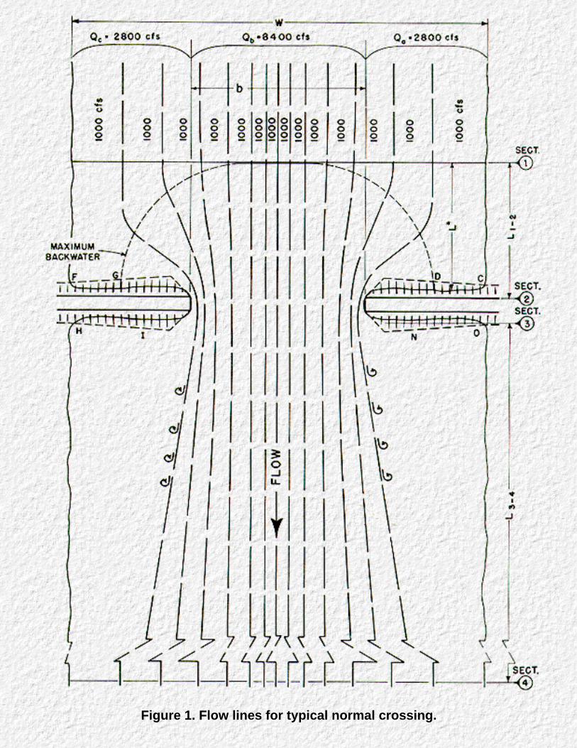
Figure 1. Flow lines for typical normal crossing.

Figure 2. Normal crossing: Wingwall abutments.

1.5 Types of Flow Encountered

There are three types of flow which may be encountered in bridge waterway design. These arelabeled types I through III on Figure 4. The long dash lines shown on each profile representnormal water surface, or the stage the design flow would assume prior to placing a constriction inthe channel. The solid lines represent the configuration of the water surface, on centerline ofchannel in each case, after the bridge is in place. The short dash lines represent critical depth, orcritical stage in the main channel (Y1c and Y4c) and critical depth within the constriction, Y2c, forthe design discharge in each case. Since normal depth is shown essentially the same in the fourprofiles, the discharge, boundary roughness, and slope of channel must all increase in passingfrom type I to type IIA, to type IIB, to type III flow.

Type I Flow

Referring to Figure 4A, it can be observed that normal water surface is everywhere above criticaldepth. This has been labeled type I or subcritical flow, the type usually encountered in practice.With the exception of Chapter 10, and example 11, all design information in this publication islimited to type I (subcritical flow). The backwater expression for type I flow is obtained byapplying the conservation of energy principle between sections 1 and 4. The method of analysisis presented in Section A.1, Appendix A.

Type IIA Flow

There are at least two variations of type II flow which will be described here under types IIA andIIB. For type IIA flow, Figure 4B, normal water surface in the unconstricted channel againremains above critical depth throughout but the water surface passes through critical depth in theconstriction. Once critical depth is penetrated, the water surface upstream from the constriction,and thus the backwater, becomes independent of conditions downstream (even though the watersurface returns to normal stage at section 4). Thus the backwater expression for type I flow is notvalid for type II flow.

Type IIB Flow

The water surface for type IIB flow, Figure 4C, starts out above both normal water surface andcritical depth upstream, passes through critical depth in the constriction, next dips below criticaldepth downstream from the constriction and then returns to normal. The return to normal depthbe rather abrupt as in Figure 4C, taking place in the form of a poor hydraulic jump, since normalwater surface in the stream is above critical depth. A backwater expression applicable to bothtypes IIA and IIB flow has been developed by equating the total energy between section 1 andthe point at which the water surface passes through critical stage in the constriction. (SeeSection A.2, Appendix A.)

Type III Flow

In type III flow, Figure 4D, the normal water surface is everywhere below critical depth and flowthroughout is supercritical. This is an unusual case requiring a steep gradient but such conditionsdo exist, particularly in mountainous regions. Theoretically backwater should not occur for thistype, since the flow throughout is supercritical. It is more than likely that an undulation of thewater surface will occur in the vicinity of the constriction, however, as indicated on Figure 4D.

1.6 Field Verification

The first edition of this bulletin was prepared principally from the results of model studies verifiedby several backwater measurements taken by the U.S. Geological Survey during floods onmedium size bridges. The field structures measured up to 220 feet in length with flood plains aswide as 0.5 mile. A summary of this information is contained in the comprehensive model studyreport (18). It was presumed that design information could be used in the range prescribed withconfidence. The applicability of the information to structures with larger width to depth ratiosremained to be proven.

Since publication of the first edition, the U.S. Geological Survey has made additional fieldmeasurements during floods at an assortment of bridges. These measurements were sponsoredby the Mississippi Highway Department and the Bureau Public Roads and were made at bridgesup to 2,100 feet in length in the State of Mississippi. Flood plains were generally heavilyvegetated and extremely wide which boosted the width to depth ratios, formerly limited to 112, toover 700. A summary of the field data to date is included in Table B-1, Table B-2, and Table C-1.

The recently acquired field data have indicated that the model studies are only partially valid typeI flow. This was principally due to the width to depth limitation. For bridge opening ratios (Section1.10) less than M = 0.55, the flow in the model could change from type I to type II, but regardlessof the value of the contraction ratio M, all field structures investigated in the State of Mississippioperated well within the subcritical range. It was thus necessary to revise the former backwaterbase curve, Figure 6, and some others. Where changes in the former design curves have beenmade, mention is made of this fact in the appropriate chapter and explanations and datasupporting these changes are included in Appendix B. To maintain continuity and brevity in thedesign procedure, extraneous material has been reserved for the appendixes.

The changes incorporated in this edition are in the backwater coefficient curve (Figure 6), thedistance to maximum backwater curve (Figure 13), and dual bridges (Figure 14 and Figure 15).Figure 10 for skewed crossings and Figure 12 for differential level across embankments havebeen changed only in format to facilitate their use. New sections have been added on partiallyinundated bridges and flow over roadway (Chapter 8), spur dikes (Chapter 9), and backwatercoefficients for type II flow (Chapter 10).

1.7 Definition of Symbols

Most of the symbols used in this publication are recorded here for reference. Symbols not foundhere are defined where first mentioned.A1 = Area of flow including backwater at section 1 (Figure 2B and Figure 3B) (sq. ft.).

An1 = Area of flow below normal water surface at section 1 (Figure 2B and Figure 3B)(sq. ft.).

An2 = Gross area of flow in constriction below normal water surface at section 2 (Figure2C and Figure 3C)(sq. ft.).

A4 = Area of flow at section 4 at which normal water surface is reestablished (Figure2A) (sq. ft.).

Ap = Projected area of piers normal to flow (between normal water surface andstreambed) (sq. ft.).

As = Area of scour measured on downstream side of bridge (sq. ft.).

α = Area of flow in a subsection of approach channel (sq. ft.).B = Width of test flume or for field structures.

b = Width of constriction (Figure 2C, Figure 3C, and Section 1.8) (ft.).bs = Width of constriction of a skew crossing measured along centerline of roadway

(Figure 9) (ft.).

C = h18*/h1* = Correction factor for backwater with scour.

Cb = Backwater coefficient for flow type II.

Cf = Freeflow coefficient for flow over roadway embankment.

Cs = Submergence factor for flow over roadway.

Db = = Differential level ratio.

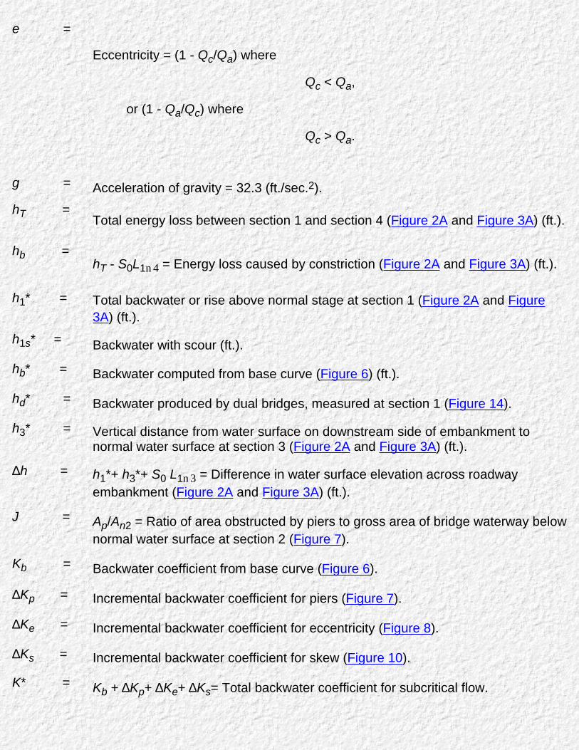
e =

Eccentricity = (1 - Qc/Qa) where

Qc < Qa,

or (1 - Qa/Qc) where

Qc > Qa.

g = Acceleration of gravity = 32.3 (ft./sec.2).hT =

Total energy loss between section 1 and section 4 (Figure 2A and Figure 3A) (ft.).

hb =hT - S0L1n4 = Energy loss caused by constriction (Figure 2A and Figure 3A) (ft.).

h1* = Total backwater or rise above normal stage at section 1 (Figure 2A and Figure3A) (ft.).

h1s* = Backwater with scour (ft.).

hb* = Backwater computed from base curve (Figure 6) (ft.).

hd* = Backwater produced by dual bridges, measured at section 1 (Figure 14).

h3* = Vertical distance from water surface on downstream side of embankment tonormal water surface at section 3 (Figure 2A and Figure 3A) (ft.).

∆h = h1*+ h3*+ S0 L1n3 = Difference in water surface elevation across roadwayembankment (Figure 2A and Figure 3A) (ft.).

J = Ap/An2 = Ratio of area obstructed by piers to gross area of bridge waterway belownormal water surface at section 2 (Figure 7).

Kb = Backwater coefficient from base curve (Figure 6).

∆Kp = Incremental backwater coefficient for piers (Figure 7).

∆Ke = Incremental backwater coefficient for eccentricity (Figure 8).

∆Ks = Incremental backwater coefficient for skew (Figure 10).

K* = Kb + ∆Kp+ ∆Ke+ ∆Ks= Total backwater coefficient for subcritical flow.

k = Conveyance in subsection of approach channel.kb = Conveyance of portion of channel within projected length of bridge at section 1

(Figure 2B and Figure 3B and Section 1.9).

ka, kc = Conveyance of that portion of the natural flood plain obstructed by the roadwayembankments (subscripts refer to left and right side, facing downstream) (Figure2B and Figure 3B and Section 1.9).

K1 = Total conveyance at section 1 (Section 1.9).

L1-4 = Distance from point of maximum back water to reestablishment of normal watersurface downstream, measured along centerline of stream (Figure 2A and Figure3A) (ft.).

L1-3 = Distance from point of maximum backwater to water surface on downstream sideof roadway embankment (Figure 2A and Figure 3A)(ft.).

L1-2 = Distance from point of maximum backwater to upstream face of bridge deck(Figure 2A and Figure 3A) (ft.).

L* =Distance from point of maximum backwater to water surface on upstream side ofroadway embankment, measured parallel to centerline of stream (Figure 13) (ft.).

Ld = Distance between upstream face of first bridge and downstream face of secondbridge (dual bridges) (ft.).

l = Overall width of roadway or bridge (ft.).M = Bridge opening ratio (Section 1.10).n = Manning roughness coefficient (Table 1).

p = Wetted perimeter of a subsection of a channel (ft.).Qb = Flow in portion of channel within projected length of bridge at section 1 (Figure 1)

(c.f.s.).Qa,Qc = Flow over that portion of the natural flood plain obstructed by the roadway

embankments (Figure 1) (c.f.s.).

Q = Qa+ Qb+ Qc = Total discharge (c.f.s.).

r = a/p = Hydraulic radius of a subsection of flood plain or main channel (ft.).S0 = Slope of channel bottom or normal water surface.

V1 = Q/A1 = Average velocity at section 1 (ft./sec.).

V4 = Q/A4 = Average velocity at section 4 (ft./sec.).

Vn2 = Q/An2 = Average velocity in constriction for flow at normal stage (ft./sec.).

V2c = Critical velocity in constriction (ft./sec.).

wp = Width of pier normal to direction of flow (Figure 7) (ft.).

W = Surface width of stream including flood plains (Figure 1) (ft.).y1 = Depth of flow at section 1 (ft.).

y4 = Depth of flow at section 4 (ft.).

yn = Normal depth of flow in model (ft.).

= An2/b= Mean depth of flow under bridge, referenced to normal stage, (Figure 3C)(ft.).

y1c = Critical depth at section 1 (ft.).

y2c = Critical depth in constriction (ft.).

y4c = Critical depth at section 4 (ft.).

α1 = Velocity head coefficient at section 1 (Section 1.11) (Greek letter alpha).

α2 = Velocity head coefficient for constriction (Greek letter alpha).

η =hd*/h1* = Backwater multiplication factor for dual bridges (Greek letter eta).

σ = Multiplication factor for influence of M on incremental backwater coefficient forpiers (Figure 7B) (Greek letter sigma).

ψh = h2*+ h3* = for single bridge (Greek letter psi).

ψh3B = hd*+ h3B* = Term used in computing difference in water surface elevation acrosstwo embankments (dual crossings) (Figure 14).

= ψh3B/ψh = Differential level multiplication factor for dual bridges (Section 5.3).(Greek letter phi).

ω = Correction factor for eccentricity (Figure 13) (Greek letter omega).

φ = Angle of skew-degrees (Figure 9) (Greek letter phi).

SPUR DIKESLs = Length of spur dike (ft.) (Figure 30).

Qf = Lateral or flood plain flow (c.f.s.).

Q100 = Discharge confined to 100 feet of stream width adjacent to bridge abutment(c.f.s.).

100 = Average depth of flow in 100 feet of stream adjacent to bridge abutment.

Qf /Q100 = Spur dike discharge ratio.

Figure 3. Normal crossings: Spillthrough abutments.

Figure 4. Types of flow encountered.

1.8 Definition of Terms

Specific explanation is given below with respect to the concept of several of the terms andexpressions frequently used throughout the discussion:

Normal Stage:

Normal stage is the normal water surface elevation of a stream at a bridge site, for a particulardischarge, prior to constricting the stream (see Figure 2A and Figure 3A). The profile of the watersurface is essentially parallel to the bed of the stream.

Abnormal Stage:

Where a bridge site is located upstream from, but relatively close to, the confluence of twostreams, high water in one stream can produce a backwater effect extending for some distanceup the other stream. This can cause the stage at a bridge site to be abnormal, meaning higherthan would exist for the tributary alone. An abnormal stage may also be caused by a dam,another bridge, or some other constriction downstream. The water surface with abnormal stageis not parallel to the bed (Figure 16).

Normal Crossings:

A normal crossing is one with alignment at approximately 90° to the general direction of flowduring high water (as shown in Figure 1).

Eccentric Crossing:

An eccentric crossing is one where the main channel and the bridge are not in the middle of theflood plain (Figure 8).

Skewed Crossing:

A skewed crossing is one that is other than 90° to the general direction of flow during flood stage(Figure 9).

Dual Crossing:

A dual crossing refers to a pair of parallel bridges, such as for a divided highway (Figure 14).

Multiple Bridges:

Usually consisting of a main channel bridge and one or more relief bridges.

Width of Constriction, b:

No difficulty will be experienced in interpreting this dimension for abutments with vertical facessince b is simply the horizontal distance between abutment faces. In the more usual caseinvolving spillthrough abutments, where the cross section of the constriction is irregular, it issuggested that the irregular cross section be converted to a regular trapezoid of equivalent area,as shown in Figure 3C. Then the length of bridge opening can be interpreted as:

Width to depth ratio:

Defined as width of flood plain to mean depth in constriction

1.9 Conveyance

Conveyance is a measure of the ability of a channel to transport flow. In streams of irregularcross section, it is necessary to divide the water area into smaller but more or less regularsubsections, assigning an appropriate roughness coefficient to each and computing thedischarge for each subsection separately. According to the Manning formula for open channelflow, the discharge in a subsection of a channel is:

By rearranging:

where k is the conveyance of the subsection. Conveyance can, therefore, be expressed either interms of flow factors or strictly geometric factors. In bridge waterway computations, conveyanceis used as a means of approximating the distribution of flow in the natural river channel upstream

from a bridge. The method will be demonstrated in the examples of Chapter 12. Totalconveyance k1 is the summation of the individual conveyances comprising section 1.

1.10 Bridge Opening Ratio

The bridge opening ratio, M, defines the degree of stream constriction involved, expressed asthe ratio of the flow which can pass unimpeded through the bridge constriction to the total flow ofthe river. Referring to Figure 1,

(1)

or,

The irregular cross section common in natural streams and the variation in boundary roughnesswithin any cross section result in a variation in velocity across a river as indicated by the streamtubes in Figure 1. The bridge opening ratio, M, is most easily explained in terms of discharges,but it is usually determined from conveyance relations. Since conveyance is proportional todischarge, assuming all subsections to have the same slope, M can be expressed also as:

(2)

1.11 Kinetic Energy Coefficient

As the velocity distribution in a river varies from a maximum at the deeper portion of the channelto essentially zero along the banks, the average velocity head, computed as (Q/A1)2/2g for thestream at section 1, does not give a true measure of the kinetic energy of the flow. A weightedaverage value of the kinetic energy is obtained by multiplying the average velocity head, above,by a kinetic energy coefficient, α1, defined as:

(3a)

Where:

v = average velocity in a subsection.q = discharge in same subsection.Q = total discharge in river.

V1 = average velocity in river at section 1 or Q/A1.

Figure 5. Aid for Estimating α2

The method of computation will be further illustrated in the examples in Chapter 12.

A second coefficient, α2, is required to correct the velocity head for nonuniform velocitydistribution under the bridge,

(3b)

where v, q, and Q are defined as above but apply here to the constricted cross section and

V2 = average velocity in constriction = Q/A2.

The value of α1 can be computed but α2 is not readily available for a proposed bridge. The bestthat can be done in the case of the latter is to collect, tabulate and compare values of α2 fromexisting bridges. This has been done and values of both α1 and α2 are tabulated in columns 13and 14 of Table B-2. The information for determining α2 was obtained from current metertraverses and soundings taken from the downstream side of bridges by the USGS. Figure 5,relating α2 to α1 and the contraction ratio, M, is supplied for estimating purposes only. The valueof α2 is usually less than α1 for a given crossing, but this is not always the case. Actually, thereshould be no definite relation between the two, but there is a trend. Local factors at the bridgeshould also be considered such as asymmetry of flow, variation in cross section, and extent ofvegetation in the bridge opening. Perhaps the best advice for estimating α2 is to lean toward the

generous side. The construction of the chart shown on Figure 5 is described in Section B.3,Appendix B.

Go to Chapter 2

Chapter 2 : HDS 1Computation of Backwater

Go to Chapter 3

2.1 Expression of Backwater

Bridge backwater analysis is far from simple regardless of the method employed. Many minor as well as majorvariables are involved in any single waterway problem. For the model which was installed in a rectangular flumeand operated with uniform roughness, minor variables such as type and geometry of abutments, width ofabutments, slope of embankments, roadway widths and width to depth ratio could be evaluated in relation tothe Froude Number as was done in the comprehensive model study report (18). In the case of bridges in thefield where roughness of flood plain and main channel differ materially and channel cross sections are irregular,the Froude number as was done in the comprehensive model study report(18). In the case of bridges in thefield where roughness of flood plain and main channel differ materially and channel cross sections are irregular,the Froude Number is no longer a meaningful parameter and minor variables lose their significance. This isespecially true as bridge length is increased. Fortunately, reasonable accuracy is acceptable in most bridgebackwater solutions; thus, a practical method, utilizing the dominant variables, is presented in this chapter forcomputing backwater produced by bridge constrictions.

A practical expression for backwater has been formulated by applying the principle of conservation of energybetween the point of maximum backwater upstream from the bridge, section 1, and a point downstream fromthe bridge at which normal stage has been reestablished, section 4 (Figure 2A). The expression is reasonablyvalid if the channel in the vicinity of the bridge is essentially straight, the cross sectional area of the stream isfairly uniform, the gradient of the bottom is approximately constant between section 1 and section 4, the flow isfree to contract and expand, there is no appreciable scour of the bed in the constriction, and the flow is in thesubcritical range.

The expression for computation of backwater upstream from a bridge constricting the flow, which is developedin the comprehensive report (18), is as follows:

(4)

Where:h1* = total backwater (ft.).K* = total backwater coefficient.α1 &α2

= as defined in expression 3a and 3b (see Section1.11).

An2 = gross water area in constriction measured belownormal stage (sq. ft.).

Vn2 = average velocity in constriction or Q/An2 (f.p.s.). Thevelocity, Vn2, is not an actual measurable velocity, butrepresents a reference velocity readily computed forboth model and field structures.

A4 = water area at section 4 where normal stage isreestablished (sq. ft.).

A1 = total water area at section 1, including that producedby the backwater (sq. ft.).

To compute backwater, it is necessary to obtain the approximate value of h1* by using the first part of theexpression (4):

(4a)

The value of A1 is the second part of expression (4), which depends on h1*, can then be determined and the second term ofthe expression evaluated:

(4b)

This part of the expression represents the difference in kinetic energy between sections 4 and 1, expressed interms of the velocity head, V2n2/2g. Expression (4) may appear cumbersome, but this is not the case.

Since the comprehensive report (18) is generally not available, a concise explanation regarding thedevelopment of the above backwater expression and the losses involved is included in Appendix A of thisbulletin under type I flow.

2.2 Backwater Coefficient

Two symbols are interchangeably used throughout the text, and both are backwater coefficients. The symbol Kbis the backwater coefficient for a bridge in which only the backwater coefficient for a bridge in which only thebridge opening ratio, M, is considered. This is known as a base coefficient and the curves on Figure 6 arecalled base curves. The value of the overall backwater coefficient, K*, is likewise dependent on the value of Mbut also affected by:

Number, size, shape, and orientation of piers in the constriction,1.

Eccentricity or asymmetric position of bridge with respect to the valley cross section, and2.

Skew (bridge crosses stream at other than 90° angle).3.

It will be demonstrated that K* consists of a base curve coefficient, Kb, to which is added incrementalcoefficients to account for the effect of piers, eccentricity and skew. The value of K* is nevertheless primarilydependent on the degree of constriction of flow at a bridge.

Figure 6. Backwater coefficient base curves (subcritical flow).

2.3 Effect of M and Abutment Shape (Base Curves)

Figure 6 shows the base curves for backwater coefficient, Kb, plotted with respect to the opening ratio, M, forwingwall and spillthrough abutments. Note how the coefficient, Kb, increases with channel constriction. Thelower curve applies for 45° and 60° wingwall abutments and all spillthrough types. Curves are also included for30° wingwall abutments and for 90° vertical wall abutments for bridges up to 200 feet in length. These shapescan be identified from the sketches on Figure 6. Seldom are bridges with the latter type abutments more than200 feet long. For bridges exceeding 200 feet in length, regardless of abutment type, the lower curve isrecommended. This is because abutment geometry becomes less important to backwater as a bridge islengthened. The base curve coefficients of Figure 6 apply to crossings normal to flood flow and do not includethe effect produced by piers, eccentricity and skew. Since the backwater coefficient base curve, Figure 6, hasbeen modified in this book, the reasoning and the supporting data for making this change have been placed inSection B.1, Appendix B.

2.4 Effect of Piers (Normal Crossings)

Backwater caused by introduction of piers in a bridge constriction has been treated as an incrementalbackwater coefficient designated ∆Kp, which is added to the base curve coefficient Kb when piers are present inthe waterway. The value of the incremental backwater coefficient, ∆Kp, is dependent on the ratio that the areaof the piers bears to the gross area of the bridge opening, the type of piers (or piling in the case of pile bents),the value of the bridge opening ratio, M, and the angularity of the piers with the direction of flood flow. The ratioof the water area occupied by piers, Ap, to the gross water area of the constriction, An2, both based on thenormal water surface, has been assigned the letter J. In computing the gross water area, An2, the presence ofpiers in the constriction is ignored. The incremental backwater coefficient for the more common types of piersand pile bents can be obtained from Figure 7. By entering chart A with the proper value of J and reading

upward to the proper pier type, ∆K is read from the ordinate. Obtain the correction factor, σ, from chart B foropening ratios other than unity. The incremental backwater coefficient is then:

∆Kp = σ∆K

The incremental backwater coefficients for pile bents can, for all practical purposes, be considered independentof diameter, width, or spacing of piles but should be increased if there are more than 5 piles in a bent. A bentwith 10 piles should be given a value of ∆Kp about 20 percent higher than that shown for bents with 5 piles. Ifthere is a possibility of trash collecting on the piers, or piles, it is advisable to use a larger value of J tocompensate for the added obstruction. For a normal crossing with piers, the total backwater coefficientbecomes:

K* = Kb (Figure 6) + ∆Kp (Figure 7)

Figure 7. Incremental backwater coefficient for piers.

Figure 8. Incremental backwater coefficient for eccentricity.

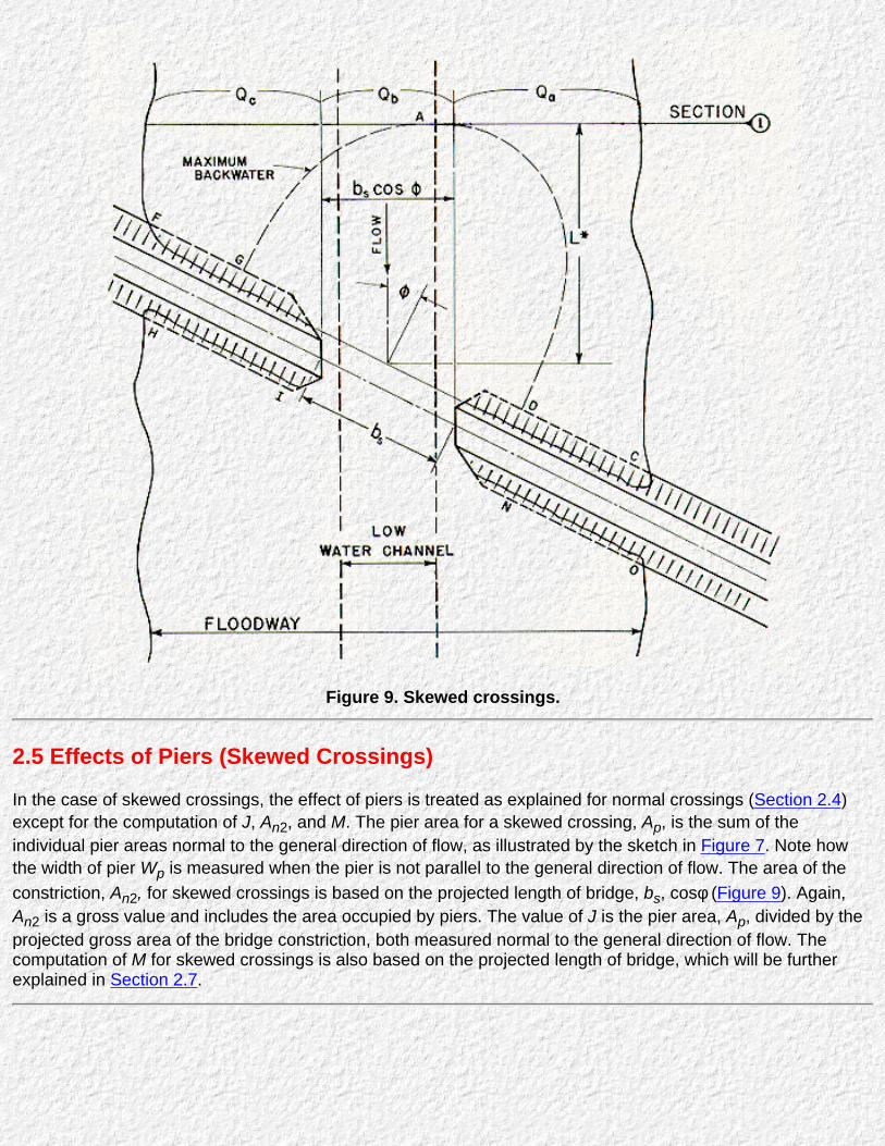
Figure 9. Skewed crossings.

2.5 Effects of Piers (Skewed Crossings)

In the case of skewed crossings, the effect of piers is treated as explained for normal crossings (Section 2.4)except for the computation of J, An2, and M. The pier area for a skewed crossing, Ap, is the sum of theindividual pier areas normal to the general direction of flow, as illustrated by the sketch in Figure 7. Note howthe width of pier Wp is measured when the pier is not parallel to the general direction of flow. The area of theconstriction, An2, for skewed crossings is based on the projected length of bridge, bs, cosφ (Figure 9). Again,An2 is a gross value and includes the area occupied by piers. The value of J is the pier area, Ap, divided by theprojected gross area of the bridge constriction, both measured normal to the general direction of flow. Thecomputation of M for skewed crossings is also based on the projected length of bridge, which will be furtherexplained in Section 2.7.

2.6 Effect of Eccentricity

Referring to the sketch in Figure 8, it can be noted that the symbols Qa and Qc at section 1 were used torepresent the portion of the discharge obstructed by the approach embankments. If the cross section isextremely asymmetrical so that Qa is less than 20 percent of Qc or vice versa, the backwater coefficient will besomewhat larger than for comparable values of M shown on the base curve. The magnitude of the incrementalbackwater coefficient, ∆Ke, accounting for the effect of eccentricity, is shown in Figure 8. Eccentricity, e, isdefined as 1 minus the ratio of the lesser to the greater discharge outside the projected length of the bridge, or:

(5)

or

Reference to the sketch in Figure 8 will aid in clarifying the terminology. For instance, if Qc/Qa = 0.05, theeccentricity e = (1 - 0.05) or 0.95 and the curve for e = 0.95 in Figure 8 would be used for obtaining ∆Ke. Thelargest influence on the backwater coefficient due to eccentricity will occur when a bridge is located adjacent toa bluff where a flood plain exists on only one side and the eccentricity is 1.0. The overall backwater coefficientfor an extremely eccentric crossing with wingwall or spillthrough abutments and piers will be:

K* = Kb (Figure 6) + ∆Kp (Figure 7) + ∆Ke (Figure 8).

Figure 10. Incremental backwater coefficient for skew.

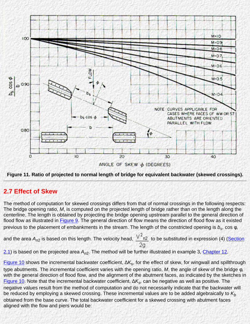
Figure 11. Ratio of projected to normal length of bridge for equivalent backwater (skewed crossings).

2.7 Effect of Skew

The method of computation for skewed crossings differs from that of normal crossings in the following respects:The bridge opening ratio, M, is computed on the projected length of bridge rather than on the length along thecenterline. The length is obtained by projecting the bridge opening upstream parallel to the general direction offlood flow as illustrated in Figure 9. The general direction of flow means the direction of flood flow as it existedprevious to the placement of embankments in the stream. The length of the constricted opening is bs, cos φ,

and the area An2 is based on this length. The velocity head, to be substituted in expression (4) (Section

2.1) is based on the projected area An2. The method will be further illustrated in example 3, Chapter 12.

Figure 10 shows the incremental backwater coefficient, ∆Ks, for the effect of skew, for wingwall and spillthroughtype abutments. The incremental coefficient varies with the opening ratio, M, the angle of skew of the bridge φ,with the general direction of flood flow, and the alignment of the abutment faces, as indicated by the sketches inFigure 10. Note that the incremental backwater coefficient, ∆Ks, can be negative as well as positive. Thenegative values result from the method of computation and do not necessarily indicate that the backwater willbe reduced by employing a skewed crossing. These incremental values are to be added algebraically to Kbobtained from the base curve. The total backwater coefficient for a skewed crossing with abutment facesaligned with the flow and piers would be:

K* = Kb (Figure 6) + ∆Kp (Figure 7) + ∆Ks (Figure 10A).

It was observed during the model testing that skewed crossings with angles up to 20° produced no particularlyobjectionable results for any of the abutment shapes investigated. As the angle increased above 20°, however,the flow picture deteriorated; flow concentrations at abutments produced large eddies, reducing the efficiency ofthe waterway and increasing the possibilities for scour. The above statement does not apply to cases where abridge spans most of the stream with little constriction.

Figure 11 was prepared from the same model information as Figure 10A. By entering Figure 11 with the angleof skew and the projected value of M, the ratio bs cos φ/b can be read from the ordinate. Knowing b and h1* fora comparable normal crossing, one can solve for bs, the length of opening needed for a skewed bridge toproduce the same amount of backwater for the design discharge. The chart is especially helpful for estimatingand checking and its use will be demonstrated in example 3, Chapter 12.

Go to Chapter 3

Chapter 3 : HDS 1Difference in Water Level across Approach Embankments

Go to Chapter 4

3.1 Significance

The difference in water surface elevation between the upstream and downstream side of bridgeapproach embankments, ∆h, has been interpreted erroneously as the backwater produced by abridge. This is not the backwater as the sketch on Figure 12 will attest. The water surface atsection 3, measured along the downstream side of the embankment, is lower than normalstage by the amount h3*. There is an occasional exception to this, however, when flow isobstructed from returning to the flood plain by dense vegetation or high water from adownstream tributary produces ponding and an abnormal stage at the bridge site.

The difference in level across embankments, ∆h, is always larger than the backwater, h1*, bythe sum h3*+ S0 L1n3, where S0 is the natural slope of the stream (Figure 12). The method ofdetermining L1n3, which is the distance from sections 1 to 3, needs specific explanation, butthis will be deferred until Chapter 4. The differential level is significant in the determination ofbackwater at bridges in the field since ∆h is the most reliable head measurement that can bemade. Fortunately, the backwater and ∆h bear a definite relation to each other for any particularstructure. Thus, if one is known, the other can be determined.

3.2 Base Curves

A base curve for determining downstream levels was constructed entirely from model datawhich was found especially consistent when presented by the parameters shown. Nosatisfactory way has been found to experimentally isolate the backwater from ∆h when makingfield measurements, so in this case the model curves must suffice. The differential level ratio,hb*/hb*+h3*, is plotted with respect to the opening ratio, M on Figure 12.

The numerator, hb*, represents the backwater at a bridge, exclusive of pier effect, and h3* isthe difference in level between normal stage and the water surface on the downstream side ofthe embankment at section 3. The ordinate of Figure 12 will be referred to as the differentiallevel ratio to which the symbol Db has been assigned. The water surface depicted at section 3represents the average level along the downstream side of the embankment from H to I and Nto O in Figure 1. For crossings involving wide flood plains and long embankments, thedistances H to I and N to O each have been arbitrarily limited or to not more than two bridgelengths. The solid curve on Figure 12 is to be used for 45° and 60° wingwall abutments and allspillthrough abutments regardless of bridge length. The upper curve, denoted by the broken

line, is for bridges with lengths up to 200 feet having 90° vertical wall and other abutmentshapes which severely constrict the flow.

Assuming the backwater, hb*, has already been computed for a normal crossing, without piers,eccentricity or skew, the water surface on the downstream side of the embankment is obtainedby entering the curve on Figure 12 with the contraction ratio, M, and reading off the differentiallevel ratio

or

(6)

The elevation on the downstream side of the embankment is simply normal stage at section 3,less h3* (Figure 12), except for the special case where the entire water surface profile is shiftedupward by ponding from downstream or restricted flood plains.

Figure 12. Differential water level ratio base curves.

3.3 Effects of Piers

As piers were introduced in the bridge constrictions in the model, it was found that thebackwater increased while the value of h3* showed no measurable change regardless of thevalue of J (Section 2.4). Therefore, the procedure for determining h3* with piers is exactly asexplained in Section 3.2 without piers.

3.4 Effect of Eccentricity

In the case of severely eccentric crossings, the difference in level across the embankmentconsidered here applies only to the side of the river having the greater flood plain discharge. Inplotting the experimental differential level ratios with respect to M for eccentric crossings,without piers, it was found that the points fell directly on the base curve (Figure 12). Theindividual values of hb* and h3* for eccentric conditions are different than for symmetricalcrossings, but the ratio of one to the other, for any given value of M, remains unchanged. Thus,Figure 12 can also be considered applicable to eccentric crossings if used correctly. To obtainh3* for an eccentric crossing, with or without piers, enter the proper curve in Figure 12 with thevalue of M and read Db as before. In this case:

or

(7)

3.5 Drop in Water Surface Across Embankment (Normal Crossing)

Having computed h3* as described in the preceding paragraphs and knowing the totalbackwater h1* (computed according to the procedure in Chapter 2), the difference in watersurface elevation across the embankment (Figure 12) is:

∆h = h3* + h1* + S0L1-3 (8)

where h1* is total backwater, including the effect of piers and eccentricity, and S0 L1n3 is thenormal fall in streambed from sections 1 to 3.

3.6 Water Surface on Downstream Side of Embankment (SkewedCrossing)

The differential level across roadway embankments for skewed crossings is naturally differentfor opposite sides of the river, the amount depending on the configuration of the stream, bendsin the vicinity of the crossing, the degree of skew, etc. These factors can be so variable that ageneralized model study can shed little light on the subject.

Individual values of h1* and h3* for skewed crossings again differ from those for symmetricalcrossings, but the differential level ratio across the embankments at either end of the bridgecan be considered the same as for normal crossings for any given value of M. The value of Mis, of course, based on the projected length of bridge as explained in Section 2.7. Thus, it isagain possible to use Figure 12 for skewed crossings. The differential level ratio, Db, with orwithout piers, is obtained by entering the chart with the proper opening ratio, M. Then:

(9)

The results for the left embankment in the model or side farthest downstream (Figure 9) weremore reliable than those for the right embankment, farthest upstream, due to the limited widthof the test flume. The results were fairly consistent, however, and the experimental points fellslightly to both sides of the base curve (Figure 12) for both wingwall and spillthroughabutments. The water surface elevations along the upstream side of the embankments (Figure9) from D to C were consistently higher than for the opposite upstream side F to G. Likewise,the water surface elevations along the downstream side of the embankments were higher fromN to O than for the right bank H to I. The difference in level across embankments, however,was essentially the same for both sides of the river. Data for the above can be found in thecomprehensive report (18).

Go to Chapter 4

Chapter 4 : HDS 1Configuration of Backwater

Go to Chapter 5

4.1 Distance to Point of Maximum Backwater

In backwater computations, it will be found necessary in some cases to locate the point orpoints of maximum backwater with respect to the bridge. The maximum backwater in line withthe midpoint of the bridge occurs at point A (Figure 13B), this point being a distance, L*, fromthe waterline on the upstream side of the embankment. Where flood plains are inundated andembankments constrict the flow, the elevation of the water surface throughout the areas ABCDand AEFG will be essentially the same as at point A, where the backwater measurement wasmade on the models. This characteristic has been verified from field measurements made bythe U.S. Geological Survey on bridges where the flood plains on each side of the main channelwere no wider than twice the bridge length and hydraulic roughness was relatively low. Thecomprehensive report (18) contains further discussion of this feature.

For crossings with exceptionally wide, rough flood plains, this essentially level ponding may notoccur. Flow gradients may exist along the upstream side of the embankments due to borrowpits, ditches and cleared areas along the right-of-way. These flow gradients alongembankments are likely to be more pronounced on the falling than on the rising stage of aflood. A correlation is needed between the water level along the upstream side ofembankments and point A since it is difficult to obtain water surface elevations at point A in thefield during floods. For the purpose of design and field verification, it has been assumed thatthe average water surface elevation along the upstream side of embankments, for as much astwo bridge lengths adjacent to each abutment (F to G and D to C), is the same as at point A(Figure 13B).

Figure 13. Distance to maximum backwater.

4.2 Normal Crossings

Figure 13 has been prepared for determining distance to point of maximum backwater,measured normal to centerline of bridge. The chart differs from the one presented in the firstedition, which was based entirely on model data applicable to only a very limited portion of theproblem. The curves on Figure 13 of this book were developed from information supplied by theU.S. Geological Survey on a number of field structures during floods. The resulting chart isconsidered superior to the former one although there still remains room for improvement asadditional field data become available. The method of revision is explained in Section B.2,Appendix B.

Referring to Figure 13, the normal depth of flow under a bridge is defined here as = An2/b,where An2 is the cross sectional area under the bridge, referred to normal water surface, and bis the width of waterway. A trial solution is required for determining the differential level across

embankments, ∆h, but from the result of the backwater computation it is possible to make a fairestimate of ∆h. To obtain distance to maximum backwater for a normal channel constriction,enter Figure 13A with appropriate value of ∆h/ and and obtain the corresponding value ofL*/b. Solving for L*, which is the distance from point of maximum backwater (point A) to thewater surface on the upstream side of embankment (Figure 13B), and adding to this theadditional distance to section 3, which is known, gives the distance L1n3, Then the computeddifference in level across embankments is

∆h = h1* + h3* + S0L1-3 (8)

Should the computed value of ∆h differ materially from the one chosen, the above procedure isrepeated until assumed and computed values agree. Generally speaking, the larger thebackwater at a given bridge the further will point A move upstream. Of course, the value of L*also increases with length of bridge.

4.3 Eccentric Crossings

Eccentric crossings with extreme asymmetry perform much like one half of a normalsymmetrical crossing with a marked contraction of the jet on one side and very little contractionon the other. For cases where the value of e (Section 2.6) is greater than 0.70, enter theabscissa on Figure 13A with ∆h/ and and read off the corresponding value of L*/b asusual. Next multiply this value of L*/b by a correction factor, ω, which is obtained from Figure13C. For example, suppose ∆h/ = 0.20, = 10 and e = 0.88, the corrected value would beL*/b = 0.84 X 1.60. Distance to maximum backwater is then L*= 1.34b with eccentricity.

4.4 Skewed Crossings

In the case of skewed crossings, the water surface elevations along opposite banks of a streamare usually different than at point A; one may be higher and the other lower depending on theangle of skew, the configuration of the approach channel, and other factors. To obtain theapproximate distance to maximum backwater L* for skewed crossings (Figure 9), the sameprocedure is recommended as far normal crossings except the ordinate of Figure 13 is read asL*/bs, where bs, is the full length of skewed bridge (Figure 9).

Go to Chapter 5

Chapter 5 : HDS 1Dual Bridges

Go to Chapter 6

5.1 Arrangement

With the advent of divided highways, dual bridges of essentially identical design, placed paralleland only a short distance apart, are now common. The backwater produced by dual bridges isnaturally larger than that for a single bridge, yet less than the value which would by consideringthe two bridges separately. As the combinations of dual bridges encountered in the field arelegion, it was necessary to restrict model tests to the simplest arrangement; namely, identicalparallel bridges crossing a stream normal to the flow (see sketch in Figure 14). The tests weremade principally with 45° wingwall abutments, but also included a limited number of thespillthrough type, both having embankment slopes of 1½:1. The distance between bridges waslimited by the range permissible in the model which was 10 feet or Ld / = 11 (Figure 14).

Figure 14. Backwater multiplication factor for dual bridges.

5.2 Backwater Determination

The method of testing consisted of establishing normal flow conditions, then placing one bridgeconstriction in the flume and measuring the backwater, h1*. A second bridge constriction, identicalto the first, was next placed downstream and the backwater for the combination, hd*, wasmeasured upstream from the first bridge. The ratio, hd*/h1*, thus obtained, is plotted with respectto the parameter, Ld / , on Figure 14, where is the width of bridge and Ld is the distance fromthe upstream face of the first bridge to the downstream face of the second bridge. The curve wasestablished from tests made with and without piers. The ratio, hd*/h1*, which is assigned the

symbol η, increases as the bridges are moved apart, apparently reaching a limit and thendecreases as the distance between the bridges is further increased. The range of the model wassufficient to explore only the rising portion of the curve but most cases in practice will fall withinthis range. With bridges in close proximity to one another, the flow pattern is elongated but littledifferent from that of a single bridge. As the bridges are spaced farther apart, the embankment ofthe second bridge interferes with the expanding jet from the first, which must again contract andreexpand downstream from the second bridge, producing additional turbulence and loss ofenergy.

To determine backwater for dual bridges meeting the above requirements, it is necessary first tocompute the backwater, h1*, for a single bridge, as previously outlined in Chapter 2. Thebackwater for the dual combination, measured upstream from the first bridge (Figure 14), is then:

hd* = h1*η (10)

5.3 Drop in Water Surface Across Embankments

In the case of dual bridges, the designer may wish to know the water surface elevation on thedownstream side of the roadway embankment of the first bridge, or the water surface elevation onthe downstream side of the embankment of the second bridge. Fluctuations in the water surfacebetween bridges, due to turbulence and surging, caused the measurements to be so erratic that itwas thought inadvisable to include the results here. These data are available in thecomprehensive report (18). A characteristic to be noted in this connection, however, is that thewater surface between bridges usually stands above normal stage. (See sketch in Figure 14.)

The water surface downstream from the second bridge, on the other hand, was quite stablepermitting accurate measurements. The procedure for determining the water surface levelimmediately downstream from the second bridge embankment at section 3B (see sketch in Figure14) consists of first computing h*1 and h*3 for the upstream bridge as was outlined in Chapter 2and Chapter 3, respectively. For convenience, the sum h*1+ h*3 for the single bridge is assignedthe symbol ψh. Likewise the sum h*d + h*3B for the two-bridge combination is represented by thesymbol ψh3B. The ratio of the second head differential to the first carries the symbol , or

(11)

The ratio has been plotted with respect to Ld/l on Figure 15. To obtain the drop in level ψh3B for

the dual bridge combination, it is only necessary to multiply ψh for the single bridge by the factor from Figure 15. The difference in water surface elevation between the upstream side of the first

bridge embankment and the downstream side of the second should then be:

∆h3B = ψh3B + S0L1-3 or ∆h3B = ψh + S0L1-3B (12)

Should the water surface level on the downstream side of the second bridge embankment atsection 3B be desired relative to normal stage:

h*3B= ψh3B − h*d

The left end of the curves on Figure 14 and Figure 15 are shown as broken lines since no datawere taken to definitely establish their positions in this region. The computation of backwater fordual bridges is further explained in example 2 of Chapter 12. The charts for dual bridges in thispublication differ from those in the first edition for reasons discussed in Section B.4, Appendix B.

Figure 15. Differential level multiplication factor for dual parallel bridges.

Go to Chapter 6

Chapter 6 : HDS 1Abnormal Stage-Discharge Condition

Go to Chapter 7

6.1 Definition

Up to this point, the discussion has concerned streams flowing at normal stage; i.e., the naturalflow of the stream has been influenced only by the slope of the bed and the boundaryresistance along channel bottom and flood plains. Sometimes the stage at a bridge site is notnormal but is increased by unnatural backwater conditions from downstream. A generalbackwater curve may be produced, beginning at the confluence of tributary and main stream orat a dam, and may extend a considerable distance upstream if the stream gradient is flat.Where bridges are placed close to the confluence of two streams, abnormally highstage-discharge conditions can be of importance in design. For example, if a stream canalways be counted on to flow at abnormally high stage during floods at a particular bridge site,the increased waterway area may permit a shorter bridge than would be possible undernormal-stage conditions. To take advantage of the situation, the length of bridge would bedetermined on the basis of

the minimum abnormal stage expected which would produce the largest backwaterincrement, or

1.

the maximum expected abnormal stage which may produce the highest stage upstream.2.

Since estimating the design stage at a bridge site under abnormal conditions can be acomplicated process, requiring much individual judgment, the approach to the computation ofbackwater in this case has been treated strictly as an approximate solution or a case where it ismore important to understand the problem than to attempt precise computations. (Seereference 17 for general backwater types.)


Tests were made by first establishing normal flow in the test flume as usual, without aconstriction. The tailgate was then adjusted to increase the depth of flow by, say, 10 percent forthe same discharge, after which a centerline profile was obtained. The resulting water surfaceis labeled "abnormal stage" in Figure 16. Abutments were then placed in the flume and asecond centerline profile was made of the water surface. The difference between the secondwater surface measurement and the previous one at abnormal stage, both made at section 1, isdefined as the backwater h*1A. Similar backwater measurements were made for other degreesof bridge constriction and for depths of flow up to 40 percent greater than normal stage byregulating the tailgate. Since the backwater analysis as developed is based on flow at normalstage, expression (4) (Section 2.1) is, strictly speaking, not valid for abnormal stage-discharge

conditions. The results described in this chapter apply specifically to a model on approximatelya 1:40 scale with channel slope of 0.0012 and a Manning roughness factor of 0.024. Theresults do shed some light on this phase of the backwater problem, and an approximatesolution may, in many cases, be preferable to none.

6.3 Backwater Expression

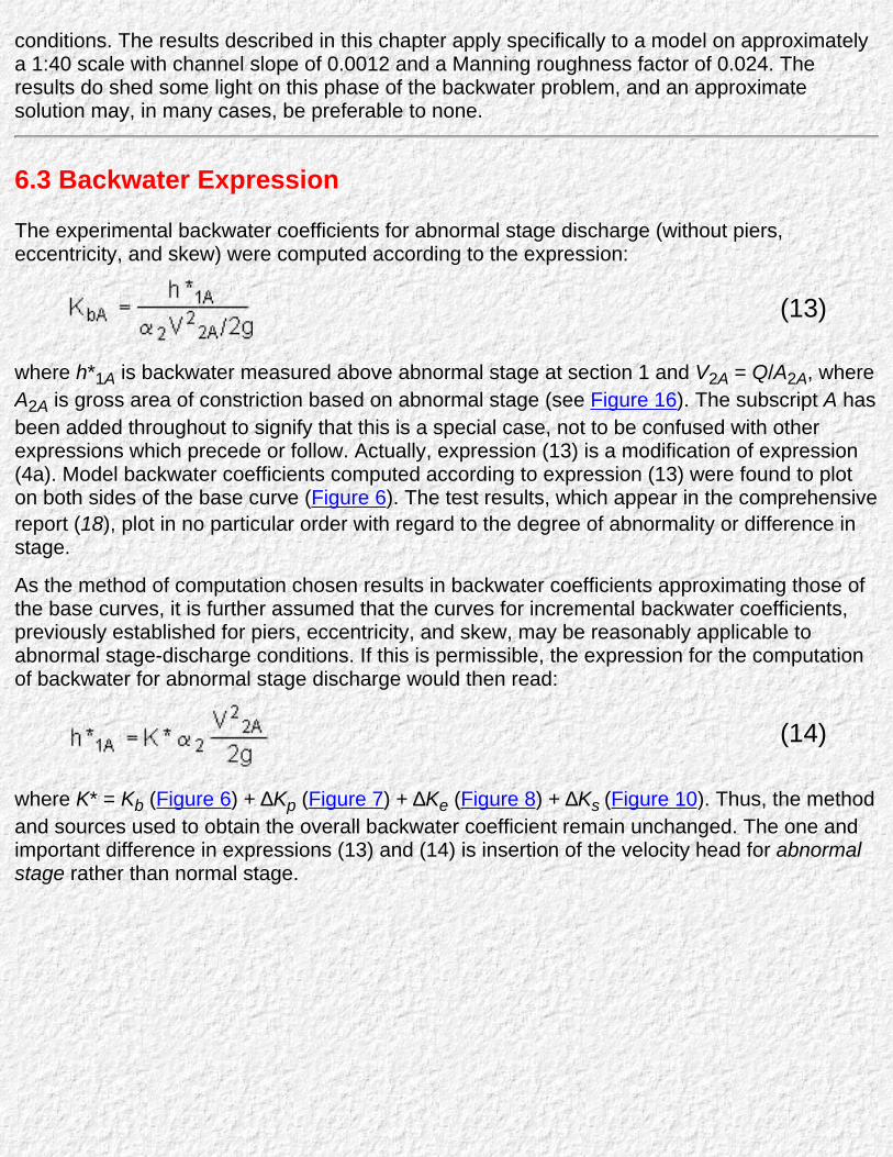
The experimental backwater coefficients for abnormal stage discharge (without piers,eccentricity, and skew) were computed according to the expression:

(13)

where h*1A is backwater measured above abnormal stage at section 1 and V2A = Q/A2A, whereA2A is gross area of constriction based on abnormal stage (see Figure 16). The subscript A hasbeen added throughout to signify that this is a special case, not to be confused with otherexpressions which precede or follow. Actually, expression (13) is a modification of expression(4a). Model backwater coefficients computed according to expression (13) were found to ploton both sides of the base curve (Figure 6). The test results, which appear in the comprehensivereport (18), plot in no particular order with regard to the degree of abnormality or difference instage.

As the method of computation chosen results in backwater coefficients approximating those ofthe base curves, it is further assumed that the curves for incremental backwater coefficients,previously established for piers, eccentricity, and skew, may be reasonably applicable toabnormal stage-discharge conditions. If this is permissible, the expression for the computationof backwater for abnormal stage discharge would then read:

(14)

where K* = Kb (Figure 6) + ∆Kp (Figure 7) + ∆Ke (Figure 8) + ∆Ks (Figure 10). Thus, the methodand sources used to obtain the overall backwater coefficient remain unchanged. The one andimportant difference in expressions (13) and (14) is insertion of the velocity head for abnormalstage rather than normal stage.

Figure 16. Backwater with abnormal stageCdischarge condition.

6.4 Drop in Water Surface Across Embankments

The experimental points for the differential level ratio for abnormal stage discharge (withoutpiers) were also found to agree fairly well with the base curve (Figure 12). The information isincluded in the comprehensive report (18). To obtain the water surface along the downstreamside of the roadway embankment for abnormal stage discharge, Figure 12 is consideredapplicable but approximate. The method of computation is similar to that explained in Chapter3; the principal differences lie in the manner in which the backwater is computed for abnormalstage conditions. Other symbols involved in the abnormal stage-discharge computation alsobear the subscript A, so the differential level ratio:

(15)

or

(16)

where:

Db = differential level ratio from base curve, Figure 12 (no adjustment is needed foreccentricity or skew);

h*bA = backwater above abnormal stage (without piers);

h*3A = vertical distance from water surface to abnormal stage at section 3 (thisdimension will be the same with or without piers).

Except for minor revisions, the reporting of this chapter on abnormal stage discharge is thesame as that which appeared in the original publication. The above procedures for bridgebackwater computation with abnormal stage will be demonstrated in example 5 of Chapter 12.

Go to Chapter 7

Chapter 7 : HDS 1Effect of Scour on Backwater

Go to Chapter 8

7.1 General

Thus far the discussion of backwater has been limited to the case where the bed of a stream in the vicinity ofa bridge is considered rigid or immovable and, thus, does not degrade with introduction of embankments,abutments, and piers. It was necessary to obtain the initial experimental data under more or less idealconditions before introducing the further complication of a movable bed. In actuality, the bed is usuallycomposed of much loose material, some of which will move out of the constriction during flood flows. Naturewastes little time in attempting to restore the former regime, or the stage-discharge relation which existedprior to constriction of the stream. For within-bank flow little changes, but for flood flows there exists analtered regime, with a potential to enlarge the waterway area under the bridge.

Bearing in mind that during floods a stream is usually transporting sediment at its capacity, the processmight be described as follows, with the aid of Figure 17. Constriction of a stream produces backwater atflood flows; backwater is indicative of an increase in potential energy upstream. This makes possible highervelocities in the constriction, thus, increasing the transport capacity of the flow to above normal in this reach.The greater capacity for transport results in scouring of the bed in the vicinity of the constriction; theremoved material is usually carried a short distance downstream and dropped as the stream again returns tofull width. As the scouring action proceeds, the waterway area under the bridge enlarges, the velocity andresistance to flow decreases, and a reduction in the amount of backwater results. If the bed is composed ofalluvial material, free to move, and a flood persists for a sufficient period of time, degradation under thebridge may approach a state of equilibrium; e.g., the scour hole can reach such proportions that the rate oftransport out of the hole is matched by the rate of transport into the hole from upstream. Upon reaching thisstate of equilibrium, it will be found that the stream has been practically restored to its former regime so faras stage discharge is concerned and the backwater has all but disappeared. This state could be fullyrealized in the model operating under controlled conditions.

Seldom is it possible to reach this extreme state in the field where backwater becomes negligible ascohesive, compacted, and cemented soils are encountered together with boulders and vegetation whichmaterially retard the scouring process. Also, the stage of most rivers in flood does not remain constant forany appreciable length of time. Nevertheless, now that information is available for the extreme case ofequilibrium scour, this should be of value in predicting the lesser scour at field structures. In cases whereabutments and piers can be keyed into bedrock, it may be advisable to encourage scour in the interest ofutilizing a shorter bridge. This same objective is sometimes attained in another way by enlarging thewaterway area under a bridge by excavation during construction. In such cases, it is desirable to be able todetermine the amount of backwater to be expected after localized enlargement of the waterway. There isalways the possibility, however, that deposition may refill the excavated channel to essentially its originalcondition. Maintaining a channel as constructed is not easily accomplished.

7.2 Nature of Scour

It is advisable to mention a few of the characteristics of scour, as observed during the model experiments,prior to considering the effect of scour on backwater. Where the depth of flow is essentially uniform and thebed is composed of a narrow gradation of clean sand, as was the case in the model, scour was greatest inthe vicinity of the abutments, as shown in Figure 17B, and little scour was evidenced in the center of the

constriction unless the scour holes overlapped. This is better illustrated by a photograph of the model inFigure 18 which shows the nature of scour around a 45° wingwall abutment and at two circular piers after atest run. The zero contour line represents normal elevation of the sandbed before placing the embankmentin the flume. The remainder of the contour lines, which are at 0.2-foot intervals, define the resulting scourhole produced by initially constricting the channel 38 percent with the embankment. This photograph isincluded to demonstrate that scour in the model did not occur uniformly across the constriction, but wasgreatest at points where concentration of flow occurs. It can be noted that scour around the two circularpiers is minor compared to scour at the abutment.

Figure 19 is a cross section of the same scour hole, measured along the upstream side of the bridge. Thenormal flow depth was 0.52 foot in this case, while the maximum equilibrium scour at the abutmentamounted to twice this value. The pattern of scour experienced in the model is not necessarily indicative ofthat which will occur in a stream.

Figure 17. Effect of scour on bridge backwater.

It is not only difficult to predict the magnitude of scour, but it is equally difficult to predict the location of scour

at field structures since the depth of flow from flood plain to main channel can differ widely as well as thedirection and concentration of flow. In the model, the greatest concentration occurred at the abutments,while in the field the deeper scour may occur in the main channel as indicated in Figure 17C. Should themain flow or a secondary current be directed toward an abutment during flood, or should a concentration offlow exist near an abutment, the area adjacent to the abutment is definitely vulnerable to scour. It is not theintention here to go into detail on the vagaries of scour, since this would require much illustrative matter andexplanation, but merely to point out a few features fundamental to understanding the effect of scour onbackwater. References 20, 21, 23, 24, and 29 are recommended for the study and prediction of scour atbridge abutments and piers.

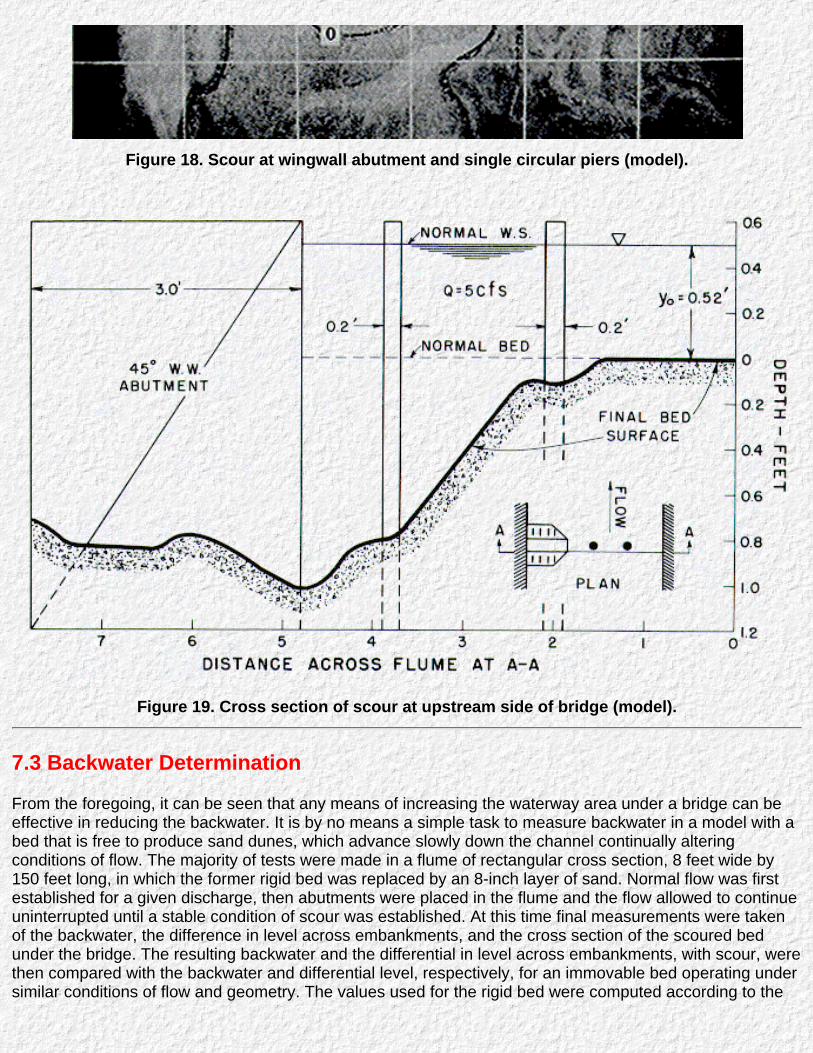
Figure 18. Scour at wingwall abutment and single circular piers (model).

Figure 19. Cross section of scour at upstream side of bridge (model).


From the foregoing, it can be seen that any means of increasing the waterway area under a bridge can beeffective in reducing the backwater. It is by no means a simple task to measure backwater in a model with abed that is free to produce sand dunes, which advance slowly down the channel continually alteringconditions of flow. The majority of tests were made in a flume of rectangular cross section, 8 feet wide by150 feet long, in which the former rigid bed was replaced by an 8-inch layer of sand. Normal flow was firstestablished for a given discharge, then abutments were placed in the flume and the flow allowed to continueuninterrupted until a stable condition of scour was established. At this time final measurements were takenof the backwater, the difference in level across embankments, and the cross section of the scoured bedunder the bridge. The resulting backwater and the differential in level across embankments, with scour, werethen compared with the backwater and differential level, respectively, for an immovable bed operating undersimilar conditions of flow and geometry. The values used for the rigid bed were computed according to the

methods outlined in Chapter 2 and Chapter 3. Holding the discharge and abutment geometry the same forany test, the reduction in backwater was related directly to the volume or cross sectional area of scour.Scour and velocity are usually measured from the downstream side of a bridge, since this is the mostpratical way of obtaining these measurements during flood flows. Also, the effective area of scour, so far asthe computation of backwater is concerned, will more likely correspond to the scour at the downstream sidethan that at the upstream side of a bridge. Thus, the area of scour measured at the downstream side,denoted as As, will be used for the computation of backwater. The model tests showed the scour at thedownstream side to average about 75 percent of that at the upstream side of the bridge.

A design curve derived from the model experiments is included as Figure 20. The correction factor forbackwater with scour (C = h*1s/h*1) is plotted with respect to As/An2 where the terms bearing the subscript s,designate values with scour; those not bearing this subscript represent the same values computed with rigidbed. Supposing the backwater at a given bridge was 1 foot with no scour; it would be reduced to 0.52-footwere scour to enlarge the waterway area by 50 percent, or it would be reduced to 0.31-foot should thewaterway area be doubled. The same reduction applies equally well to the ratios h*3s/h*3 and ψhs/ψh (seeFigure 17A) so one curve will suffice for all three. Thus to obtain backwater and related information forbridge sites where scour is to be encouraged, where scour cannot be avoided, or where the waterway is tobe enlarged during construction, it is first necessary to compute the backwater and other quantities desiredaccording to the method outline in Chapter 2 and Chapter 3 for a rigid bed, using the original cross sectionof the stream at the bridge site. These values are then multiplied by a common coefficient from Figure 20 asfollows:

h*1s = Ch*1

h*3s = Ch3*

ψhs = Cψh

(17)

(18)

(19)

7.4 Enlarged Waterways

The designer will probably be reluctant to depend on scour as a means of enlarging a waterway and therebyreducing backwater. If the waterway is enlarged by excavation, there is little to gain by excavating muchbeyond the limits (upstream or downstream) of the embankments as the downstream channel acts as thecontrol (Figure 18). If additional volume is removed upstream or downstream, the channel may simply refillby deposition. Any enlargement of the cross section should be maintained to prevent reduction of area bythe growth of willows and similar vegetation. Field surveys of existing bridges where channel enlargementshave once been made should reveal worthwhile information on the question of permanence of enlargedwaterways. Chapter 12, example 6, which is based on an actual occurrence involving a flash flood on astream with a bed consisting of non-cohesive material, is included to demonstrate how backwater is reducedby scour.

Attention is called to the well known fact that scour measured after flood waters have subsided does not givea true indication of the extent of scour which occurred during the peak of the flood. This is evidenced bymany incidents where bridge spans and piers have fallen into a stream during a flood and have been burieddeep in the bed. As flood waters recede, the transport capacity as well as the velocity of the flow drops off,with the result that material is deposited all along the streambed as well as in the constriction.

Figure 20. Correction factor for backwater with scour.

Go to Chapter 8

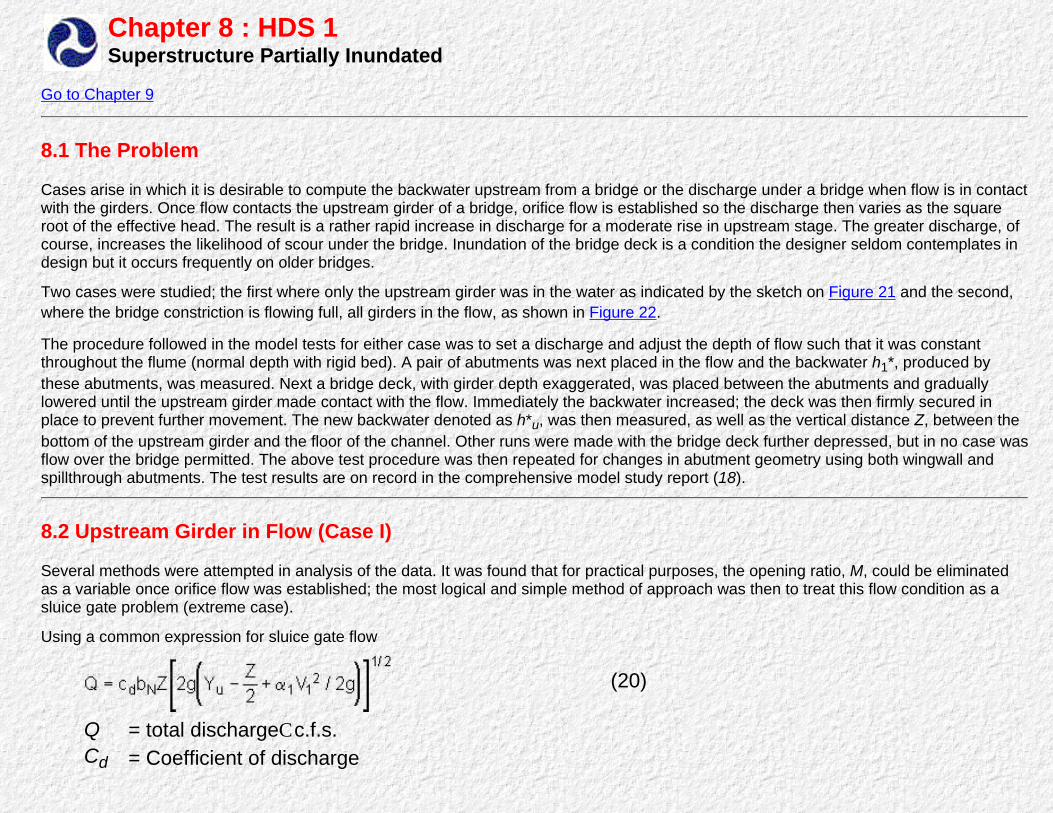
Chapter 8 : HDS 1Superstructure Partially Inundated

Go to Chapter 9

8.1 The Problem

Cases arise in which it is desirable to compute the backwater upstream from a bridge or the discharge under a bridge when flow is in contactwith the girders. Once flow contacts the upstream girder of a bridge, orifice flow is established so the discharge then varies as the squareroot of the effective head. The result is a rather rapid increase in discharge for a moderate rise in upstream stage. The greater discharge, ofcourse, increases the likelihood of scour under the bridge. Inundation of the bridge deck is a condition the designer seldom contemplates indesign but it occurs frequently on older bridges.

Two cases were studied; the first where only the upstream girder was in the water as indicated by the sketch on Figure 21 and the second,where the bridge constriction is flowing full, all girders in the flow, as shown in Figure 22.

The procedure followed in the model tests for either case was to set a discharge and adjust the depth of flow such that it was constantthroughout the flume (normal depth with rigid bed). A pair of abutments was next placed in the flow and the backwater h1*, produced bythese abutments, was measured. Next a bridge deck, with girder depth exaggerated, was placed between the abutments and graduallylowered until the upstream girder made contact with the flow. Immediately the backwater increased; the deck was then firmly secured inplace to prevent further movement. The new backwater denoted as h*u, was then measured, as well as the vertical distance Z, between thebottom of the upstream girder and the floor of the channel. Other runs were made with the bridge deck further depressed, but in no case wasflow over the bridge permitted. The above test procedure was then repeated for changes in abutment geometry using both wingwall andspillthrough abutments. The test results are on record in the comprehensive model study report (18).

8.2 Upstream Girder in Flow (Case I)

Several methods were attempted in analysis of the data. It was found that for practical purposes, the opening ratio, M, could be eliminatedas a variable once orifice flow was established; the most logical and simple method of approach was then to treat this flow condition as asluice gate problem (extreme case).

Using a common expression for sluice gate flow

(20)

Q = total dischargeCc.f.s.Cd = Coefficient of discharge

bN = net width of waterway (excluding piers)Cft.

Z = vertical distanceCbottom of upstream girder to mean river bedunder bridge

Yu= vertical distanceCupstream water surface to mean river bed atbridge ft.

For case I, the coefficient of discharge Cd, plotted with respect to the parameter Yu /Z on Figure 21. The upper curve applies to thecoefficient of discharge where only the upstream girder is in contact with the flow. By substituting values expression (20) , it is possible tosolve for either water surface upstream or the discharge under the bridge, depending on the quantities known. It appears that the coefficientcurve (Figure 21) approaches zero as Yu /Z becomes unity. This is the case since the limiting value of Yu /Z for which expression (20)applies is not much less than 1.1.There is a transition zone somewhere between Yu /Z = 1.0 and 1.1 where free surface flow channel toorifice flow or vice versa. The type of flow within this range is unpredictable. For Yu /Z = 1.0, flow is dependent on the natural slope of thestream, while this factor is of little concern after orifice flow is established or Yu /Z > 1.1.

In computing a general river backwater curve across the bridge shown on Figure 21, it is necessary to know water surface elevationdownstream as well as upstream from the bridge. The approximate depth of flow, ys, can be obtained from Figure 21 by entering the topscale with the proper value of Yu /Z and reading down to the upper curve, then over horizontally to the lower curve, and finally down to thelower scale as shown by the arrows. The lower scale gives the ratio of Yu /Y3. The method is illustrated in example 7 of Chapter 12.

Figure 21. Discharge coefficients for upstream girder in flow (case I).

Figure 22. Discharge coefficient for all girders in flow (case II).

8.3 All Girders in Contact with Flow (Case II)

Where the entire area under the bridge is occupied by the flow, the computation is handled in a different manner. To compute the watersurface upstream from the bridge, the water surface on the downstream side and the discharge must be known. Or if the discharge isdesired, the drop in water surface across the roadway embankment, ∆h, and the net area under the bridge is required. The experimentalpoints on Figure 22A, which are for both wingwall and spillthrough abutments, show the coefficient of discharge to be essentially constant at0.80 for the range of conditions tested. The equation recommended for the average two to four lane concrete girder bridge for case II is

Q = 0.80 bNZ(2g∆h)1/2 (21)

where the symbols are defined as in expression (20). Here the net width of waterway (excluding width of piers) is used again. It is preferableto measure ∆h across embankments rather than at the bridge proper. The partially inundated bridge compares favorably with that of asubmerged box culvert (14) but on a larger scale. Submergence, of course, can increase the likelihood of scour under a bridge.

Again for working up general backwater curves for a river, such as is done by the Corps of Engineers, Bureau of Reclamation, and otheragencies, it is desirable to know the drop in water level across existing bridges as well as the actual water surface elevation either upstreamor downstream from the bridge. Once ∆h is computed from expression (21), the depth of flow upstream, Yu, can be obtained from chart B.Figure 22, where is depth from normal stage to mean river bed at bridge in feet. The procedure will be further explained by example 8 ofChapter 12.

8.4 Safety of Bridge

A rather common source of bridge failure results from the superstructure being virtually pushed or lifted off the abutments and piers by thecombination of buoyancy and dynamic forces. Inundation reduces the effective weight of a concrete bridge to about 0.6 of its weight in air.Should air be trapped under the deck between girders, the effective weight can be further reduced to a dangerous limit so that onlymoderate horizontal forces are required to jar or slide bridge spans off their pedestals. The horizontal forces consist of unbalancedhydrostatic pressure, or ponding, acting on the upstream face of the bridge (aggravated by the collection of trash), plus energy inherent inmoving mass of water (32), plus impact forces produced by buildings, barges and large floating objects striking a bridge. The impact fromlarge floating objects can be lethal if the bridge is under stress and the girders are not anchored piers. The force of impact can be calculatedby equating impulse against momentum:

or

, (22)

where ∆t is time required to bring the mass W/g, floating down river at a velocity, V1, to rest upon striking a solid object. Say a woodenstructure weighing 8 tons, is carried down a swollen river at 5 ft./sec.; the force it would exert on impact depend on the resilience of the

object, the resilience of the bridge span it strikes and the manner in which it strikes. Suppose it makes a square hit so that its velocitychanges from 5 ft./sec. to zero in 0.5 second. The force of impact would be

On the other hand, assume that a mattress of trash collected on the upstream side of the offers a cushioning effect so that the time intervalfor the velocity to change from 5 ft./sec. to zero is now 2.5 seconds. This would reduce the force by five times to 994 lbs. Here is a casewhere trash can serve a useful purpose. Figure 23 shows what the combination of buoyant and horizontal forces can do to a bridge whichcan break from its supports. Air trapped under these 80-foot prestressed concrete spans and the force of the flood water against the girderscarried these two spans several hundred feet downstream from substructure and stacked them.

Section 1.7.56, entitled "Anchor Bolts" in the AASHO standard specifications for Highway Bridges, 1969, specifies that girders preferablyshall be securely anchored to the substructure. This is an inexpensive and recommended precaution. Where there is a possibility of the flowcoming in contact with the deck during heavy or unusual floods, it is recommended that girders be anchored, tied or blocked in such a waythat they cannot be pushed or lifted off their pedestals by hydraulic forces. Even the construction of blocks on the downstream end of piercaps, which could be provided at practically no extra cost, would help prevent failure caused by sliding. Buoyancy forces can be reduced byproviding air vents near the top of girders so that entrapped air may escape. In many cases, simple precautions such as these can save abridge superstructure.

Figure 23. Buoyant and horizontal forces moved these 80-foot spans downstream.

8.5 Flow over Roadway

In cases where bridge clearance is such that girders become inundated during floods, there is a good possibility that flow also occurs overportions of the approach roadway. Should it be desired to determine the discharge flowing over the roadway, a chart is included as Figure24. Credit for this work should go to Kindsvater and Sigurdson (7 and 37).

To determine the discharge flowing over a roadway, first enter curve B (Figure 24) with H/l and obtain the free flow coefficient of dischargeCf. Should the value of H/l be less than 0.15, it is suggested that Cf be read from curve A of the same figure. If submergence is present (e.g.,if H/D is larger than 0.7) enter curve C with the proper value of submergence in percent and read off the submergence factor Cs /Cf. Theresulting discharge is obtained by substituting values in the expression:

Q = Cf LH3/2 · Cs/Cf (23)

where L represents the length of inundated roadway, H is the total head upstream measured above the crown of the roadway and Cf and Csare coefficients of discharge for free flow and with submergence, respectively. Where the depth of flow varies along the roadway, it isadvisable to divide the inundated portion into reaches and compute the discharge over each reach separately. The process, of course, canbe reversed to aid in determining backwater for a combination of bridge and roadway.

The overtopping of roadways bears a connotation of the past, but this sort of thinking should not be discarded; it has far reachingpossibilities in present and future design. The present tendency, for Interstate and primary roads, is to construct approach embankmentswell above the 50-year flood, or highest flood level of record, and depend on the bridge to pass all flood waters, including the super flood. Alimit must be set on the length of bridge for economic reasons, which is usually proportioned for about a 50-year flood, but where topographyis favorable, this same bridge with embankments set at a lower predetermined level may handle a 1,000-year flood safely. An excellentexample of this type of design is the bridge across the Missouri River near Rocheport, Mo., on Interstate 70. A profile across the valleylooking upstream is shown on Figure 25. The bridge is located well above high water, the approach embankment on the left is set at aboutthe 75-year flood level, yet there is adequate sight distance throughout. This is the ideal valley cross section and the bridge andembankment have been tailor made to fit the site. The arrangement will accommodate any flood that is likely to occur with a minimum ofdamage. Computation of flow across this roadway is shown in example 9 (Chapter 12). The manner in which a crossing of this kind functionshas been explained in reference 6; a portion of the explanation is repeated in Section 8.6.

Figure 24. Discharge coefficients for flow over roadway embankments.

Figure 25. Missouri River Bridge on Route I-70.

Figure 26. Nottoway River Bridge on Virginia Route 40.

8.6 Nottoway River Bridge

The crossing of the Nottoway River on State Route 40 near Sussex, Va., is an actual case on which reliable field observations andmeasurements were made.

"The 175-ft. bridge shown in Figure 26 has withstood several severe floods, one with a recurrence interval exceeding 100 years. Thecapacity of the bridge itself is approximately 10,000 c.f.s., however, a flood of 26,000 c.f.s., or approximately 2½ times the capacity, wasaccommodated with no damage to the bridge. Only minor repairs were required to the downstream shoulders of the embankments.

"The solid line in Figure 26 represents the stage-discharge relationship for the river at the bridge site. Discharges of up to 10,000 c.f.s. werecarried under the bridge. As the stage reached El. 70, flow began to spill over the road. With flow over the roadway established, resistancedecreased, resulting in a corresponding reduction in both backwater upstream from the bridge and differential head across the embankment.In turn, reduction in backwater caused the flow under the bridge to decrease. By the time the stage reached El. 75, water flowed to a depthof 5 ft. over the roadway. Flow over the embankment at this point reached 24,000 c.f.s. whereas flow under the bridge fell to less than 2,000c.f.s.

"The backwater upstream from the bridge reached a maximum of 0.37 ft. for the stage at El. 70. The differential head across theembankment was approximately double this amount for the same stage but fell to 0.015 ft. as the stage reached El. 75. Measurementsindicated that the highest mean velocity attained under the bridge was 4 f.p.s. at approximately El. 70, decreasing to 0.7 f.p.s. as the stageapproached El. 75. The velocity over the roadway reached a maximum of approximately 2 f.p.s. at El. 70.3, decreasing to approximately 0.7f.p.s. for river stage at El. 75.

"The greatest test withstood by the bridge foundations occurred, therefore, not at the peak flow, but at 10,000 c.f.s. For greater flows, thedischarge and velocity under the bridge decreased. The greatest threat to the superstructure occurred at the peak of the flood when timberand debris lodged against it, but with the low velocities prevailing at that time even this was not serious. The outstanding factor contributingto the safety of the bridge is the sure suprisingly large capacity of the roadway when it is operating as a submerged broad-crested weir." (6)

The above case is for a rather short bridge on a secondary road involving low velocities, but the principle is the same regardless of size,provided there is sufficient width of flood plain to warrant such a design. It is recommended that this safety valve idea be kept in mind andused where applicable. The roadway in this case would be located slightly above the flood level for which the bridge is designed. The bridgeshould have sufficient clearance so that the lowest part of the superstructure remains above high water at all times.

The following comment made by F. A. Kilpatrick of the U.S.G.S. is worthy of mention here. "My observations of the Colorado 1965 floods,and the damage to the Interstate System would seem to point out the advantages of such thinking, especially where the restoration of trafficcan be accomplished as quickly as was the case in the western States. After the Colorado floods, the embankments were restored in 1 to 2days, the bridges only after many months and millions of dollars."

Go to Chapter 9

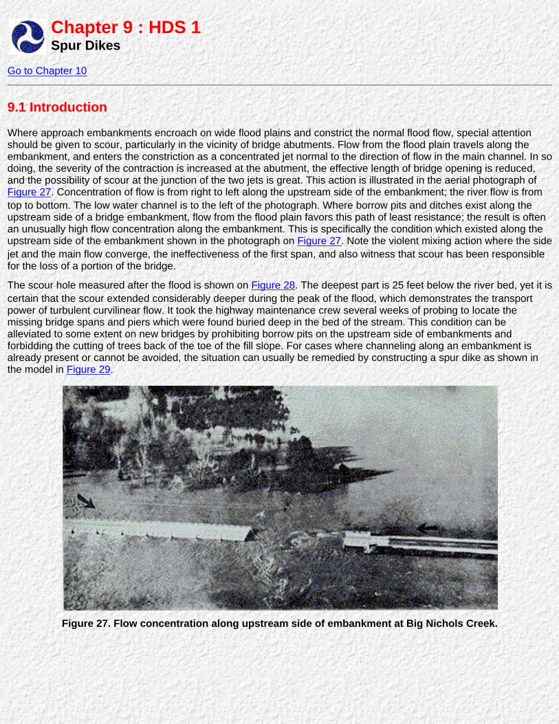
Chapter 9 : HDS 1Spur Dikes

Go to Chapter 10

9.1 Introduction

Where approach embankments encroach on wide flood plains and constrict the normal flood flow, special attentionshould be given to scour, particularly in the vicinity of bridge abutments. Flow from the flood plain travels along theembankment, and enters the constriction as a concentrated jet normal to the direction of flow in the main channel. In sodoing, the severity of the contraction is increased at the abutment, the effective length of bridge opening is reduced,and the possibility of scour at the junction of the two jets is great. This action is illustrated in the aerial photograph ofFigure 27. Concentration of flow is from right to left along the upstream side of the embankment; the river flow is fromtop to bottom. The low water channel is to the left of the photograph. Where borrow pits and ditches exist along theupstream side of a bridge embankment, flow from the flood plain favors this path of least resistance; the result is oftenan unusually high flow concentration along the embankment. This is specifically the condition which existed along theupstream side of the embankment shown in the photograph on Figure 27. Note the violent mixing action where the sidejet and the main flow converge, the ineffectiveness of the first span, and also witness that scour has been responsiblefor the loss of a portion of the bridge.

The scour hole measured after the flood is shown on Figure 28. The deepest part is 25 feet below the river bed, yet it iscertain that the scour extended considerably deeper during the peak of the flood, which demonstrates the transportpower of turbulent curvilinear flow. It took the highway maintenance crew several weeks of probing to locate themissing bridge spans and piers which were found buried deep in the bed of the stream. This condition can bealleviated to some extent on new bridges by prohibiting borrow pits on the upstream side of embankments andforbidding the cutting of trees back of the toe of the fill slope. For cases where channeling along an embankment isalready present or cannot be avoided, the situation can usually be remedied by constructing a spur dike as shown inthe model in Figure 29.

Figure 27. Flow concentration along upstream side of embankment at Big Nichols Creek.

Figure 28. Extent of scour measured after the flood at Big Nichols Creek.

9.2 Function and Geometry of Spur Dike

Where approach embankments divert considerable flood plain flow through the bridge opening, a spur dike, properlyproportioned, is effective in reducing the gradient and velocity along the embankment by moving the mixing action ofthe merging flow away from the abutment to the upstream end of the dike.

Figure 29. Model of a spur dike.

The combined flow is directed so that the entire waterway under the bridge is utilized and the depth of scour in thevicinity of the bridge abutment and at adjacent piers is reduced. Scour, if it occurs, is moved upstream away from thebridge structure as shown on Figure 29. Although any spur dike is usually helpful fit reducing scour from merging floodplain flow, a dike of proper proportions is needed to keep scour at the bridge abutment to a minimum and properly alignthe flow through the end spans of the bridge.

Three principal considerations are involved in proportioning a spur dike: geometry, height and length. Laboratorystudies (19 and 25) showed that a dike shaped in the form of a quarter of an ellipse, with ratio of major (length) tominor (offset) axes of 2.5:1 performed as well or better than any shape tested. The height of spur dike is based onanticipated high water. It should have sufficient height and freeboard to avoid overtopping and be protected from waveaction. With the exception of dikes constructed entirely of stone or earth dikes properly armored with graded stonefacing, overtopping will usually result in serious damage or complete destruction of a dike because the difference inlevel across the dike is usually sufficient to produce erosive velocities. The remaining dimension, length of dike, will beconsidered in detail in the following section. It may be said, however, that since field information on the operation ofspur dikes is meager, the tendency at present is to lean toward over design rather than under design.

9.3 Length of Spur Dike

The information for determining the length of spur dike was obtained from model studies performed at Colorado StateUniversity (19 and 25), field data collected by the U.S. Geological Survey during floods in the State of Mississippi (39),and field observations by D. E. Schneible (30) during floods. Additional model information may be found in references2 and 27 of the selected bibliography. The usable experimental and field information presently available on spur dikesis summarized in Table C-1 and plotted on Figure C-1. A discussion of the method of plotting, the variables involved,and the reliability of the data can be found in Appendix C. For design purposes, Figure C-1 has been reproduced,omitting the points, as Figure 30. The parameters are a spur dike discharge ratio, Qf /Q100, relating the flow over theleft or the right flood plain to a specific portion of the flow under the bridge, a representative velocity adjacent to theabutment of the bridge, and the length of spur dike needed. The discharge ratio is shown as the ordinate, the length ofdike as the abscissa, and the family of curves are for different values of the velocity, Vn2.

Definitions of the symbols used are:

Q = Total discharge of stream (c.f.s.).Qf = Lateral or flood plain flow (one side) measured at section 1 (c.f.s.).

Q100= Discharge in 100 feet of stream adjacent to abutment, measured at section 1(c.f.s.).

b = Length of bridge opening (ft.).An2 = Water area under bridge referred to normal stage (sq. ft.).Vn2 = Q/An2 = Average velocity through bridge opening (f.p.s.).Qf /Q100 = Spur dike discharge ratio.Ls = Top length of spur dike (measured as shown on Figure 30 (ft.).

The shape of the dike will conform to the equation of one quarter of an ellipse with 2.5:1 ratio of major to minor axis.

(24)

or

Ls = (X2 + 6.25Y2)1/2

It can be observed from Figure 30 that the length of a spur dike should be increased with an increase in flood plaindischarge, with an increase in velocity under the bridge, or both. The chart is read by entering the ordinate with theproper value of Qf /Q100, moving horizontally to the curve corresponding with the computed value of Vn2 and thendownward to obtain from the abscissa the length of spur dike required. As a general rule, if the length read from theabscissa is less than 30 feet, a spur dike is not needed. For chart lengths from 30 to 100 feet, it is recommended that aspur dike no less than 100 feet long be constructed. This length is needed to direct the curvilinear flow around the endof the dike so that it will merge with the main channel flow and establish a straight course down river before reaching

the bridge abutment. Curvilinear flow can have several times the capacity to scour than that of parallel flow, dependingon the radius of curvature, velocity, depth of flow and other factors. Holding the depth of flow and other factors thesame, the depth of scour will increase with decrease in radius of curvature. For this reason, the deepest scourproduced by a spur dike occurs near the nose where the radius of curvature is sharpest.

Figure 30. Charts for determining length of spur dikes.

Figure 31 shows a case where spur dikes are indispensable on the Tarbela Bridge on the Indus River in West Pakistan(42). The average velocity under the bridge will be about 14 f.p.s. for the design flood of 750,000 c.f.s. For bridgesskewed at an angle of 45°, it is recommended that the forward dike (see sketch, Figure 30) be lengthened by 50percent over the value given by the design chart. For lesser angles, the forward dike may be lengthened in proportion.Figure 32 shows a spur dike at a bridge on the Susquehanna River near Nanticoke, Pa., during the flood of March1964. The spur dike, which is constructed entirely of rock, is 300 feet long, and the bridge is skewed at an angle of 45°with the river. This dike was built before the model studies, therefore, it is not elliptical in plan, and the flow does notfollow the nose as well as it should. It has proven very effective, however, as evidenced by comparisons of the scour at

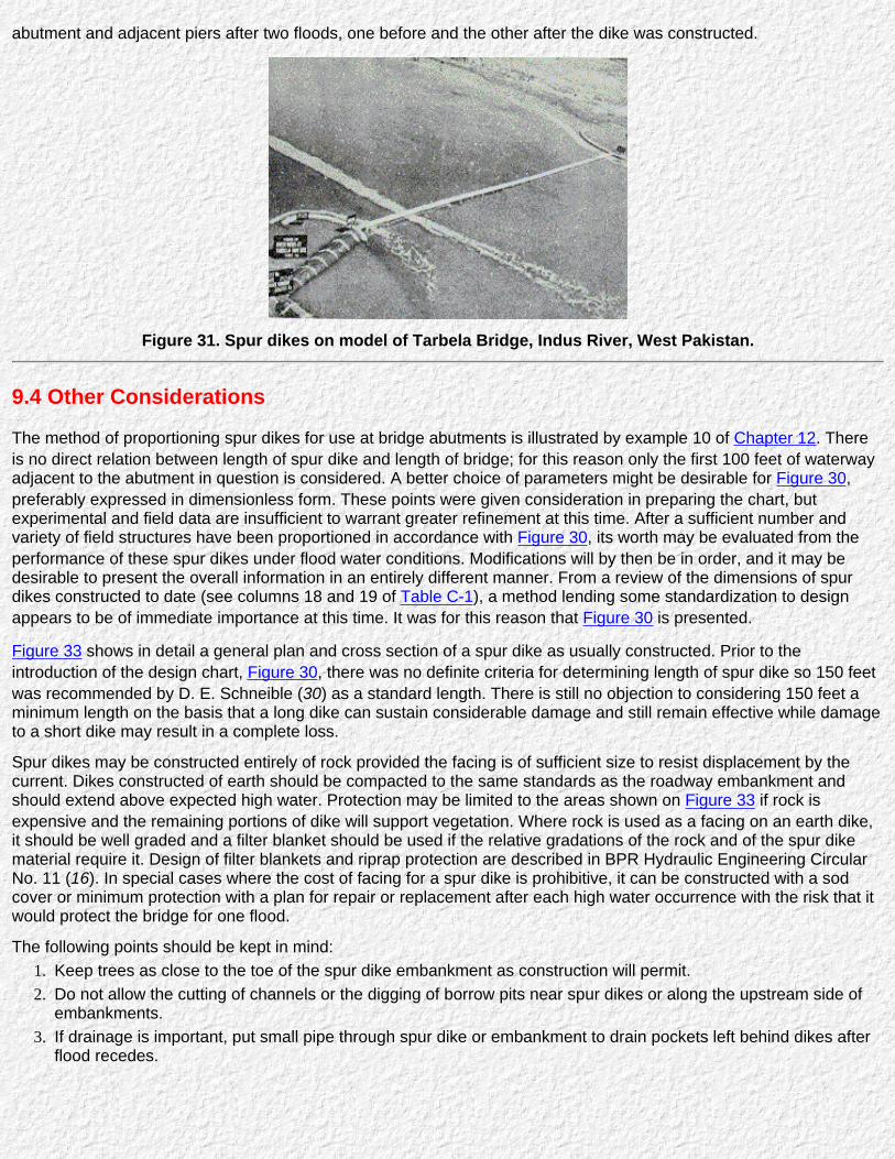
abutment and adjacent piers after two floods, one before and the other after the dike was constructed.

Figure 31. Spur dikes on model of Tarbela Bridge, Indus River, West Pakistan.

9.4 Other Considerations

The method of proportioning spur dikes for use at bridge abutments is illustrated by example 10 of Chapter 12. Thereis no direct relation between length of spur dike and length of bridge; for this reason only the first 100 feet of waterwayadjacent to the abutment in question is considered. A better choice of parameters might be desirable for Figure 30,preferably expressed in dimensionless form. These points were given consideration in preparing the chart, butexperimental and field data are insufficient to warrant greater refinement at this time. After a sufficient number andvariety of field structures have been proportioned in accordance with Figure 30, its worth may be evaluated from theperformance of these spur dikes under flood water conditions. Modifications will by then be in order, and it may bedesirable to present the overall information in an entirely different manner. From a review of the dimensions of spurdikes constructed to date (see columns 18 and 19 of Table C-1), a method lending some standardization to designappears to be of immediate importance at this time. It was for this reason that Figure 30 is presented.

Figure 33 shows in detail a general plan and cross section of a spur dike as usually constructed. Prior to theintroduction of the design chart, Figure 30, there was no definite criteria for determining length of spur dike so 150 feetwas recommended by D. E. Schneible (30) as a standard length. There is still no objection to considering 150 feet aminimum length on the basis that a long dike can sustain considerable damage and still remain effective while damageto a short dike may result in a complete loss.

Spur dikes may be constructed entirely of rock provided the facing is of sufficient size to resist displacement by thecurrent. Dikes constructed of earth should be compacted to the same standards as the roadway embankment andshould extend above expected high water. Protection may be limited to the areas shown on Figure 33 if rock isexpensive and the remaining portions of dike will support vegetation. Where rock is used as a facing on an earth dike,it should be well graded and a filter blanket should be used if the relative gradations of the rock and of the spur dikematerial require it. Design of filter blankets and riprap protection are described in BPR Hydraulic Engineering CircularNo. 11 (16). In special cases where the cost of facing for a spur dike is prohibitive, it can be constructed with a sodcover or minimum protection with a plan for repair or replacement after each high water occurrence with the risk that itwould protect the bridge for one flood.

The following points should be kept in mind:Keep trees as close to the toe of the spur dike embankment as construction will permit.1.

Do not allow the cutting of channels or the digging of borrow pits near spur dikes or along the upstream side ofembankments.

2.

If drainage is important, put small pipe through spur dike or embankment to drain pockets left behind dikes afterflood recedes.

3.

Figure 32. Spur dike on 45° skewed bridge over Susquehanna River at Nanticoke Pa.

Figure 33. Plan and cross section of spur dike.

A 14-minute motion picture (16 mm. film) entitled, "Spur Dikes," demonstrating the theory and performance of theseelliptical shaped embankments during high water, is available on loan from the Federal Highway Administration,Publications and Visual Aids Branch, Washington, D.C. 20591.

Go to Chapter 10

Chapter 10 : HDS 1Flow Passes Through Critical Depth (Type II)

Go to Chapter 11

10.1 Introduction

The computation of backwater for bridges on streams with fairly steep gradients, by the methodoutlined up to this point, may result in unrealistic values. When this occurs, it is probably a signthat the flow encountered is type II (see Figure 4), and the backwater analysis for subcritical ortype I flow no longer applies. The water surface for type IIA flow passes through critical stageunder the bridge but returns to normal or subcritical flow some distance downstream. In thecase of type IIB flow, the water surface passes through critical stage under the bridge and thendips below critical stage downstream. One analysis that applies to both types is found inSection A.2, Appendix A. The sole source of data for type II flow is from model studies, whichcover but a limited range of contraction ratios.

10.2 Backwater Coefficients

Design information for other than type I flow has been in demand and some designers haveexpressed confusion in attempting to apply the type I analysis to other types of flow. It has beendecided, therefore, to present a tentative backwater coefficient curve (Figure 34) based on theinformation at hand. The expression for the backwater coefficient in this case is:

(25)

Where:

= Normal depth in constriction or An2/b (ft.)y2c = Critical depth in constriction or A2c/b (ft.)V2c = Critical velocity in constriction or Q/A2c (f.p.s.)α2 = Velocity head coefficient for the constriction

The backwater coefficient has been assigned the symbol Cb to differentiate it from thecoefficient for subcritical flow.

The curve of Figure 34 accounts for the contraction ratio only, which is the major factor

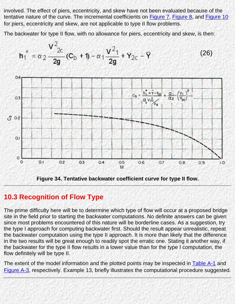
involved. The effect of piers, eccentricity, and skew have not been evaluated because of thetentative nature of the curve. The incremental coefficients on Figure 7, Figure 8, and Figure 10for piers, eccentricity and skew, are not applicable to type II flow problems.

The backwater for type II flow, with no allowance for piers, eccentricity and skew, is then:

(26)

Figure 34. Tentative backwater coefficient curve for type II flow.

10.3 Recognition of Flow Type

The prime difficulty here will be to determine which type of flow will occur at a proposed bridgesite in the field prior to starting the backwater computations. No definite answers can be givensince most problems encountered of this nature will be borderline cases. As a suggestion, trythe type I approach for computing backwater first. Should the result appear unrealistic, repeatthe backwater computation using the type II approach. It is more than likely that the differencein the two results will be great enough to readily spot the erratic one. Stating it another way, ifthe backwater for the type II flow results in a lower value than for the type I computation, theflow definitely will be type II.

The extent of the model information and the plotted points may be inspected in Table A-1 andFigure A-3, respectively. Example 13, briefly illustrates the computational procedure suggested.

Go to Chapter 11

Chapter 11 : HDS 1Preliminary Field and Design Procedures

Go to Chapter 12

11.1 Evaluation of Flood Hazards

Bureau of Public Roads' instructions require that after January 1, 1968, all Federal and Federal-aid highway plans submitted forapproval shall show the magnitude, frequency, and pertinent water surface elevations for the design flood and, if available, similar datafor the maximum flood of record for all structures and roadway embankments that cross flood plains or encroach on rivers and streamshaving a design flood of more than 500 c.f.s. Similar information for structures designed for lesser discharges are to be recorded in theproject design files. In addition, the instructions require that highway structures that encroach on or cross the flood plain of a drainagecourse shall not cause a significant adverse effect to developments on the flood plain, and at the same time the structure shall becapable of withstanding the design flood flow with minimum damage.

On interstate projects, all bridges and culverts are to accommodate floods of at least a 50-year frequency or the greatest flood ofrecord, whichever is greater, with runoff based on land development 20 years hence and backwater limited to an amount which will notresult in damage to upstream property or the highway. Where the greatest flood of record is considerably larger than the 50-year floodand the cost to provide for such an exceptional flood without damage or flooding to the roadway or adjacent property is shown byanalysis to be excessive, for the protection given, a lesser flood, but not less than the flood of 50-year frequency, may be used fordesign. The effect of flood-control structures on reducing floods should be considered in determining the design flood.

For Federal-aid projects other than interstate, similar requirements apply as in the above paragraphs except that design floods may beless than a 50-year frequency where conditions warrant lower standards. The flood frequency selected for design should be consistentwith the magnitude of damage to adjacent property and the importance of the highway.

11.2 Site Study Outline

The following outline is presented to aid in organizing and collecting the necessary field data for a bridge site investigation:Location map to show proposed highway alignment and reach of river to be studied.1.

U.S.G.S. Quadrangle sheet or map of equal detail..

Aerial photographs.b.

Vicinity map showing flood flow patterns, cross sections of stream, location of proposed bridge and relief openings, andalignment of piers.

2.

Map showing 1- or 2-foot contours, stream meanders, vegetation and manmade improvements..

In some cases, cross sections perpendicular to flood flow are acceptable in lieu of the map in (a); at least three crosssections are desirable: one on the centerline of the proposed bridge, one upstream and one downstream from the

b.

proposed bridge at from 500- to 1,000-foot intervals.A full description of existing bridges both upstream and downstream from proposed crossing (including relief and overflowstructures).

3.

Type of bridge, including span lengths and pier orientation..

Cross section beneath structure, noting stream clearance to superstructure and skew or direction of current duringfloods.

b.

All available flood history high water marks with dates of occurrence, nature of flooding, damages and source ofinformation.

c.

Photographs of existing bridges, past floods, main channels and flood plains and information as to nature of drift, ice,streambed and stability of banks.

d.

Factors affecting water stage at bridge site.4.

High water from other streams..

ReservoirsCexisting or proposed and approximate date of construction.b.

Flood control projects.c.

Tide.d.

Other controls.e.

Figure 35. Status of U.S. Geological Survey nationwide flood frequency project.

11.3 Hydrological Analysis Outline

Site inspection should be made by engineer making hydrological and hydraulic analysis.List flood records available on river being studied.1.

Determine drainage area above proposed crossing from available maps.2.

Plot flood frequency curve for the site.3.

Plot a stage-discharge curve for the site.4.

Prepare chart showing distribution of flood flow and velocities for several discharges or stages in natural channel withoutproposed bridge. (n-values used in this computation should be selected by an experienced hydraulic engineer.)

5.

The following sections contain information which may prove of value in compiling the above listed material.

11.4 Flood Magnitude and Frequency

A complete discussion of estimating flood frequency is beyond the scope of this publication, but sources of data will be cited. Thefrequency and magnitude of floods may be determined from gaging station records, if available, on the river in question. In the absenceof such records, a regional flood frequency study may be made or may already be available from studies made by the U.S. GeologicalSurvey or others.

The Geological Survey has prepared two series of water-supply papers that summarize streamflow in the United States as measuredcontinuously or periodically at stream-gaging stations. The first series of these compilation reports contains monthly data from thebeginning of record for each station through September 1950 ("Compilation of records of surface waters of the United States throughSeptember 1950"). The second series of reports contains similar data for the period October 1950 through September 1960.

Recently a nationwide series of water-supply papers was completed on the "Magnitude and frequency of floods in the United States."The reports contain tables of maximum known floods at gaging stations and curves for estimating the probable magnitude of floods offrequencies ranging up to 50 years for most streams (gaged or ungaged) for discharges not materially affected by regulation ordiversion.1 A map outlining the boundaries of the nationwide flood frequency project, recently completed, is included as Figure 35. Theheavy lines outline the geographical areas studied and the part numbers are those used in the annual reports on surface-water supplyof the United States. The number of the water supply paper applicable to each area is shown on the map together with the date ofpublication. Also indicated are locations of U.S.G.S. district and principal field offices where additional field information may beavailable. Inquiries can be made of the surface water branch office of the State in question.

The Bureau of Public Roads has made studies to determine peak rates of runoff from small watersheds. Reference 15 describes aresearch study limited to watersheds of 25 square miles or less, located east of the 105th meridian. Hydraulic Engineering Circular No.2 (12)2 describes a flood estimating procedure based on an analysis of 55 streamflow records and drainage areas ranging from 0.03 to762 square miles in the Piedmont Plateau, which embodies the area between the Appalachian Mountains and the Atlantic coastalplain, extending from Alabama to New Jersey.

1 All three series of reports are available for reference at many public and university libraries. Those reports still in print may bepurchased from the Superintendent of Documents, Government Printing Office, Washington, D.C. 20402.

2 Available in limited numbers from Office of Engineering and Operations, Bureau of Public Roads, Washington, D.C. 20591.

11.5 Stage Discharge

It is important that the normal stage of a river for the design flood be determined as accurately as possible at the bridge site. This maybe accomplished in several ways, but where possible it is best to establish it from a stage-discharge rating curve based onstream-gaging records collected in the vicinity of the bridge site. Such records are available in the files of the U.S. Geological Survey. Atypical stage-discharge curve, Figure 40, accompanies example 4 in Chapter 12. The scale at the top of the graph also shows floodrecurrence intervals. Where stage-discharge records are lacking for the stream in question, the usual procedure is to locate high watermarks of floods by consulting people who live in the vicinity of the proposed bridge site. Flood information supplied by local residents isoften inaccurate, but may be considered reliable if confirmed by other residents.

It is then necessary to find a means of relating stage to discharge. This can be done by the slope-area method, a simplified variation ofwhich will be found illustrated in example 1 and example 4. Extreme care must be exercised both in the collection of field data and inthe manner in which it is processed if glaring discrepancies are to be avoided in the final result. In many cases where records arelacking, it is advisable to arrange for the installation and maintenance of a temporary stream gage at or near the bridge site severalyears in advance of construction. Even a single reliable point at an intermediate stage can be of inestimable value in the preparation ofa stage-discharge curve.

11.6 Channel Roughness

A matter of prime importance in bridge backwater or slope-area computations is the ability to evaluate properly the roughness of themain channel and of the flood plains; both are subject to extreme variations in vegetal growth and depth of flow. As a guide, values ofthe Manning roughness coefficient, n, as commonly encountered in practice, are tabulated for various conditions of channel and floodplain in Table 1. Since the practicing engineer in this country is familiar with the Manning roughness coefficient, the Manning equationhas been chosen for use here. In interpreting roughness coefficients from Table 1, it should be kept in mind that the value of n for asmall depth of flow, especially on a flood plain covered with grass, weeds, and brush, can be considerably larger than that for greaterflow depths over the same terrain (34 and 35). On the other hand, as the stage rises in a stream with an alluvial bed, sand wavesdevelop which can increase the value of n (4). It is, therefore, suggested that the notes accompanying Table 1 be carefully consideredalong with the tabulation. An especially useful guide for choosing channel roughness coefficients is reference 41.

11.7 Bridge Backwater Design Procedure

The following is a brief step-by-step outline for determining the backwater produced by a bridge constriction:Determine the magnitude and frequency of the discharge for which the bridge is to be designed from sources cited (Section11.4).

1.

Determine the stage of the stream at the bridge site for the design discharge (Section 11.5).2.

Plot a representative cross section of stream for design discharge at section 1, if not already done under step 2. If streamchannel is essentially straight and cross section substantially uniform in the vicinity of the bridge, the natural cross section of thestream at the bridge site may be used for this purpose.

3.

Subdivide the cross section plotted in step 3 according to marked changes in depth of flow and changes in roughness. Assignvalues of Manning roughness coefficient, n, to each subsection (Table 1). Experience and careful judgment are necessary inselecting these values.

4.

Compute conveyance and then discharge in each subsection (method is demonstrated in examples).5.

Using cumulative conveyance and discharge at section 1, compute slope of stream, S0. Should the computed slope vary morethan 25 percent from the actual slope, reassign values of the roughness factor, n, and repeat conveyance computations.

6.

Determine value of kinetic energy coefficient, α1 (method is illustrated in examples, Chapter 12).7.

Plot natural cross section under proposed bridge based on normal water surface for design discharge, and compute gross waterarea (including area occupied by piers).

8.

Compute bridge opening ratio, M (Section 1.10).9.

Obtain value of Kb from base curve in Figure 6 for symmetrical normal crossings.10.

If piers are involved, compute value of J (Section 2.4) and obtain incremental coefficient, ∆Kp, from Figure 7 (note methodoutlined for skewed crossings, Section 2.5).

11.

If eccentricity is severe, compute value of e (Section 2.6) and obtain incremental coefficient, ∆Ke, from Figure 8.12.

If a skewed crossing is involved, observe proper procedure in previous steps, then obtain incremental coefficient, ∆Ke,for properabutment type from Figure 10.

13.

Determine total backwater coefficient, K*, by adding incremental coefficients to base curve coefficient, Kb.14.

Estimate α2 from Figure 5, then make allowance for any unusual topographic, vegetative or approach condition which may leadto further asymmetrical velocity distribution in the bridge constriction.

15.

Compute backwater by expression (4), Section 2.1.16.

Determine distance upstream to maximum backwater from Figure 13 and convert backwater to water surface elevation at section1 if computations are based on normal stage at bridge.

17.

It is now possible to place the above basic information on punch cards and do all or part of the above procedure and computations byelectronic computer (13).

Table 1. Manning's roughness coefficient for natural stream channels1.A. Minor streams (surface width at flood stage < 100 ft.) :2 Manning's n range

Fairly regular section:1.

Cultivated areas:2. a. Nocrop.....................................................................

0.03n0.04

b. Mature row crops..................................................... 0.035n0.045c. Mature fieldcrops.....................................................

0.04n0.05

Heavy weeds, scatteredbrush.......................................................................................

3. 0.05n0.07

Light brush and trees:34. a.winter.........................................................................

0.05n0.06

b.summer.....................................................................

0.06n0.08

Medium to dense vegetation:35. a.winter........................................................................

0.07n0.11

b.summer.....................................................................

0.10n0.16

Dense willows, summer, not bent over by current6. Cleared land with tree stumps, 100n150 per acre:7. a. nosprouts..................................................................

0.04n0.05

a. Some grass and weeds, little or nobrush.............

0.030n0.035

b. Dense growth of weeds, depth of flowmaterially greater than weedheight.........................................

0.035n0.05

c. Some weeds, light brush onbanks.......................

0.035n0.05

d. Some weeds, heavy brush onbanks....................

0.05n0.07

e. Some weeds, dense willows onbanks.................

0.06n0.08

f. For trees within channel with branchessubmerged at high stage, increase all abovevaluesby........................................................................

0.01n0.02

b. with heavy growth ofsprouts............................................................................ 0.06n0.08Heavy stand of timber, a few down trees, little undergrowth:8. a. flood depth belowbranches......................................................................... 0.10n0.12b. Flood depth reaches branches (n increases withdepth)4............................................................................ 0.12n0.16

C. Major stream (surface width at flood stage > 100 ft):Roughness coefficient is usually less than for minor streams ofsimilar description on account of less effective resistance offeredby irregular banks or vegetation on banks. Values of n may besomewhat reduced. Follow general recommendations1 if possible.The value of n for larger streams of mostly regular section, with noboulders or brush, may be in therange.................................................... 0.028n0.33

Irregular section, with pools, slight channel meander;channels (a) to (e) above, increase all valuesabout....................................

2. 0.01n0.02

Mountain streams, no vegetation in channel, banksusually steep, trees and brush along banks submergedat high stage:

3.

a. Bottom of gravel, cobbles, and fewboulders............................................................................ 0.04n0.05b. Bottom of cobbles with largeboulders............................................................................ 0.05n0.07

B. Flood plains (adjacent to natural streams):Pasture, no brush:1.

a. Short grass........................................................ 0.030n0.035b. Highgrass...........................................................

0.035n0.05

1For calculations of stage or discharge in natural stream channels, it is recommended that thedesigner consult the local District Office of the U.S. Geological survey to obtain data regarding valuesof n applicable to streams of any specific design. Where the recommended procedure is not followed,the table values may be wed as a guide.With channel or alignment other than straight loss of head by resistance forces will be increased. Asmall increase in value of n may be made to allow for the additional loss of energy.2The tentative values of n cited are principally derived from measurements made on fairly short butstraight reaches of natural streams. Where slopes calculated from flood elevations along aconsiderable length of channel, involving meanders and bends, are to he used in velocity

calculations by the Manning formula, the value of n must be increased to provide for additional loss ofenergy caused by bends. All values in the table must be so increased. The increase may be in the rangeof perhaps 3 to 15 percent.3The presence of foliage on trees and brush under flood stage will materially increase the value of n.Therefore, roughness coefficients for vegetation in leaf will be larger than for bare branches. For trees inchannel or on banks, and for brush on banks where submergence of branches increases with depth offlow, n will increase with rising stage.4For important work and where accurate determination of water profiles is necessary, the designer isurged to consult reference 41 to select n by comparison with specific conditions.

Go to Chapter 12

Chapter 12 : HDS 1Illustrative Examples

Go to Chapter 13

A better understanding of the procedures for computing bridge backwater can be gained from the illustrative examples in this chapter. Some of theprocedures to be explained in detail have been computerized (13), however, the point cannot be over emphasized that to properly appreciate andutilize the computer programs, one should first become familiar with the long hand methods. The examples deal with the following phases of design:

Example 1 comprises a simple normal crossing; the steps closely follow the outline of design procedure listed in Chapter 11.

Example 2 treats example 1 as a dual crossing.

Example 3 should help clarify the procedure recommended for skewed crossings.

Example 4 is an eccentric crossing which demonstrates how backwater computations may be systematized for a typical bridge waterwayproblem where a range in bridge length and in flood discharge is to be studied. This example serves to demonstrate that the length, andhence the cost, of a bridge at a given site varies within wide limits depending on the amount of backwater considered tolerable.

Example 5 is included to demonstrate an approximate calculation for backwater at bridge sites where abnormal stage-discharge conditionsprevail.

Example 6 illustrates how scour under a bridge affects the backwater.

Example 7 and Example 8 demonstrate how discharge or differential water level across bridge embankments can be determined whenportions of the superstructure are in the flow.

Example 9 considers favoring flow over bridge embankments to serve as a safety valve for the bridge during super floods.

Example 10 demonstrates a proposed method for the design of spur dikes at bridges.

Example 11 deals with type II flow which passes through critical stage under the bridge.

12.1 Example 1: Normal Crossing

Given:

The channel crossing shown in Figure 36 with the following information: Cross section of river at bridge site showing areas, wetted perimeters, andvalues of Manning, n; normal water surface for design = El. 28.0 ft. at bridge; average slope of river in vicinity of bridge S0 = 2.6 ft./mi. or 0.00049 ft./ft.;cross section under bridge showing area below normal water surface and width of roadway = 40 ft.

The stream is essentially straight, the cross section relatively constant in the vicinity of the bridge, and the crossing is normal to the general direction offlow.

Find.Conveyance at section 1..

Discharge of stream at El. 28.0 ft.b.

Velocity head correction coefficient, α1.c.

Bridge opening ratio, M.d.

Backwater produced by the bridge.e.

Water surface elevation on upstream side of roadway embankment.f.

Water surface elevation on downstream side of roadway embankment.g.

Figure 36. Example 1: Plan and cross section of normal crossing.

Computation (1a)

Under the conditions stated, it is permissible to assume that the cross sectional area of the stream at section 1 is the same as that at thebridge. The approach section is then divided into subsections at abrupt changes in depth or channel roughness as shown in Figure 36. Theconveyance of each subsection is computed as shown in columns 1 through 8 of Table 2 (see also Section 1.9). The summation of theindividual values in column 8 represents the overall conveyance of the stream at section 1 or K1 = 879,489. Note that the water interfacebetween subsections is not included in the wetted perimeter. Table 2 is set up in short form to better demonstrate the method. The actualcomputation would involve many subsections corresponding to breaks in grade or changes in channel roughness.

Computation (1b)

Since the slope of the stream is known (2.6 ft./mi.) and the cross sectional area is essentially constant throughout the reach underconsideration, it is permissible to solve for the discharge by what is known as the slope-area method or:

Q = K1/So1/2 =879,489 (0.00049)1/2 = 19,500 c.f.s.

It should be noted that the procedure in example 3 and example 4 conforms more nearly to what is usually required in practice.

Computation (1c)

To compute the kinetic energy coefficient (Section 1.11), it is first necessary to complete columns 9, 10, and 11 of Table 2; then, usingexpression (3a) (Section 1.11):

where Σgv2 where is the summation of column 11, and Vn1 represents the average velocity for normal stage at section 1.

Table 2. Example 1: Sample ComputationsS0 = 0.0049

Subsection

Computation (1a) Computation (1c)__________________________________________________________________

n 1.49n

α p r = αp

r2/3k= 1.49

n ar2/3 q =Q kK1

v = qa

qv2

sq. ft. ft. ft. cfs fps (1) (2) (3) (4) (5) (6) (7) (8) (9) (10) (11)

Qa........... { 0-200200-240240-280

0.045.070.070

33.021.221.2

627.4285.2324.5

200.240.140.1

3.1347.1128.092

2.1423.6984.031

44,34922,35927,732

983.3495.7614.8

1.571.741.89

2,4241,5012,196

Qb.......... { 280-420420-445

.035

.05042.529.7

2,004.0205.8

145.025.1

13.8218.199

5.7594.066

490,49224,852

10,875.2551.0

5.432.68

320,6543,958

Qc.......... { 445-500500-750

.050

.04529.733.0

539.41,677.4

55.1251.0

9.7896.683

4.5763.548

73,309196,396

1,625.44,354.6

3.012.60

14,72629,436

---------An=5,663.7 sq. ft.

---------K1=879,489

---------Q=19,500.0 c.f.s

---------Σqv2=374,895

________________________________________________________________________________________

An2=2,534 sq. ft. Qb=12,040 c.f.s.

Computation (1d)

The sum of the individual discharges in column 9 must equal 19,500 c.f.s. The factor M, as stated in Section 1.10, is the ratio of that portionof the discharge approaching the bridge in width b, to the total discharge of the river, using expression (1) (Section 1.10):

Entering Figure 5 with α1 = 1.62 and M = 0.62, the value of α2 is estimated as 1.40.

Computation (1e)

Entering Figure 6 with M = 0.62, the base curve coefficient is Kb = 0.72 for bridge waterway of 205 ft.

As the bridge is supported by five solid piers, the incremental coefficient (∆Kp) for this effect will be determined as described in Section 2.4.Referring to Figure 36 and Table 2, the gross water area under the bridge for normal stage, An2, is 2,534 sq. ft. and the area obstructed bythe piers, Ap, is 180 sq. ft.;

so:

Entering Figure 7A with J = 0.071 for solid piers, the reading from ordinate is ∆K = 0.13. This value is for M = 1.0. Now enter Figure 7B andobtain the correction factor σ, for M = 0.62 which is 0.84. The incremental backwater coefficient for five piers, ∆Kp = ∆Kσ = 0.13 x 0.84 =0.11.

The overall backwater coefficient:

K* = Kb + ∆Kp = 0.72 + 0.11 = 0.83,

and

Using expression (4a) (Section 2.1), the approximate backwater will be:

(4a)

Substituting values in the second half of the expression (4) for difference in kinetic energy between sections 4 and 1 (Section 2.1) whereAn1 = 5664 sq. ft. = A4,

A1 = 6384 sq. ft., and An2 = 2534 sq. ft.,

(4b)

or

Then total backwater produced by the bridge ish1* = 1.07 +0.06 = 1.13 ft. (4)

Computation (1f)

The statement was made (in Section 4.1) that the water surface on the upstream side of the roadway embankment will be essentially thesame as that at section 1. Thus, to determine the backwater elevation it is first necessary to locate the position of section 1, which isaccomplished with the aid of Figure 13.

From preceding computations:

b = 205 ft.

and

.

It is necessary to assume the total drop across the embankments for a first trial (∆h is assumed as 1.9 ft.). Entering Figure 13 with

and

= 12.36,

and

L*=0.78 x 205 = 160 ft.

The drop in channel gradient between sections 1 and centerline of roadway is then S0 L1n = 0.00049 (160 + 30) = 0.093 ft. The watersurface elevation at section 1 and along the upstream side of the roadway embankment will be:

El. 28.0 + S0L1 - + h*1= 28.0 +0.09 + 1.13

= El. 29.2 ft.

Computation (1g)

The first step in determining the water surface elevation at section 3 is to compute the backwater for the bridge in question without piers, asexplained in Chapter 3:

Entering Figure 12 with M = 0.62, the differential level ratio for the bridge (without piers) is:

so

. (6)

The placing of piers in a waterway results in no change in the value of h*3 provided other conditions remain the same (Section 3.3),so h*3(with piers) also equals 0.67 ft. The water surface elevation on the downstream side of the roadway embankment will be essentially

El. 28.0 - 0.67 = 27.33 ft.

The drop in water surface across the embankment is then

∆h = 29.22 - 27.33 = 1.89 ft.

Since ∆h was assumed as 1.90 ft., the computed water surface elevations above are satisfactory. Should the computed value of ∆h bematerially different from that assumed, another trial will be necessary.

12.2 Example 2: Dual Bridges

Given.

A second bridge, identical to that of example 1, is to be constructed parallel and 300 feet, between centerlines, downstream from the first bridge. Thestream is essentially straight and of uniform cross section throughout this reach. Assuming no erosion at the constriction.

Find.The backwater upstream from the first bridge for a flood of 19,500 c.f.s..

The water surface elevation along upstream side of roadway embankment of the first bridge.b.

The water surface elevation along downstream side of roadway embankment of second bridge (assuming elevation of roadway the same for bothbridges).

c.

Computation (2a)

From example 1,

M = 0.62,h*1 = 1.13 ft.,J = 0.071,S = 0.00049,b = 205 ft.,An2 = 2,534 sq. ft.,An1 = 5,664 sq. ft.,h*3 = 0.67 ft.,

= 12.36 ft. andI = 40 ft.

The parameter

Entering Figure 14 with Ld / of 8.50, the backwater multiplication factor η = 1.49. The backwater upstream from the first bridge for thecombination is then:

h*d = ηh*1 = 1.49 X 1.13 = 1.68 ft.

Computation (2b)

With normal stage of El. 28.0 ft. given at site of upstream bridge, it is necessary to determine drop in channel between centerline of firstbridge and a new section 1. Assuming ∆h in this case as 2.80,

Entering Figure 13 with the above value and =12.36, L*/b = 0.92 and L* = 0.92 X 205 = 188 ft. The fall in the channel between section 1

and centerline of first bridge is S0 L1n = 0.00049 (188 + 30) = 0.11. The water surface elevation at section 1 and along the upstream sideof the roadway embankment of the first bridge will be:

EL. 28.0 + S0L1- + hd*

= 28.0 + 0.11 + 1.68

= El. 29.8 ft.

Computation (2c)

Entering Figure 15 with Ld / = 8.50, the differential level multiplication factor, ξ = ψh3B /ψh = 1.41. For the single bridge in example 1:

ψh = h*1 + h*3 = 1.13 + 0.67 = 1.80 ft.

For the two bridges

ψh3B = ξψh = 1.41 X 1.80 = 2.54 ft.L1n3B = 188 + 300 + 40 = 528 ft.S0 L1n3B= 0.00049 X 528 = 0.26 ft.∆h3B = ψh3B + S0 L1n3B = 2.54 + 0.26

= 2.80 ft.Checking back, the assumed value of ∆h3B was 2.80 feet so there is no need for repetition. The approximate water surface elevation on thedownstream side of the second bridge will be

El. 29.79 - ∆h3B = 29.79 - 2.80 = 27.0 feet.

12.3 Example 3: Skewed Crossing

Suppose it is decided to construct a skewed bridge, Figure 37, on the site chosen in example 1, rather than the normal crossing.

Given.

The quantities from example 1;

Q = 19,500 c.f.s. for N.W.S. = 28.0, b = 205, S0 = 0.00049, α1 = 1.62, M = 0.62, A4 = 5,664 sq. ft., A1 = 6,384 sq. ft. and I = 40 ft.

Find.Length of skewed bridge required to produce essentially 1.1 feet of backwater as occurred in example 1..

The backwater for bridge length chosen.b.

The approximate water level at point A on section 1.c.

Computation (3a)

The design discharge and normal stage at bridge site are known. The same procedure demonstrated in example 1 is followed, withexceptions as noted. First, the general direction of flow in the river at the bridge site for the design flood, without constriction, is determined.Next, the position and extent of roadway embankments and the type of abutment are superimposed on the stream as illustrated in Figure 9.The angle of skew is measured, which is 40° in this case; then the bridge opening is projected upstream, normal to the direction of flow, tosection 1.

Entering Figure 11, which has been reproduced from reference 3, with φ = 40° and M = 0.62.

,

bs Cos φ = 0.935 X 205 = 192 ft.,

and

Computation (3b)

The actual backwater produced by the skewed bridge, 250 feet long, will be computed as a check on the above determination as well as todemonstrate the method of procedure. Conveyance and area are both plotted with respect to distance across flood plain at section 1 onFigure 38. The information needed to construct the chart came directly from Table 2 which was prepared in connection with the solution ofexample 1.

The first step is to locate the position of the skewed bridge on Figure 38 and lay off the projected length, bs Cos φ, as shown. Then M iscomputed as follows:

From Figure 6, the backwater coefficient, Kb = 0.77. Note that an extra pier has been added and all are parallel to the direction of flow. Thearea obstructed by piers, Ap, is now 220 sq. ft. The projected area under the bridge referenced to normal water surface, from Figure 38 is

An2s = 3,400 - 1,000 = 2,400 sq. ft.

and

Consulting Figure 7, the incremental backwater coefficient for piers

∆Kp = 0.18 X 0.8 = 0.15.

Entering Figure 10A with M = 0.60 and φ = 40°,

∆Ks = - 0.19.

The total backwater coefficient for the skewed bridge is thenK*= Kb+ ∆Kp + ∆Ks = 0.77 + 0.15 - 0.19

= 0.73,

V2n2/2g=1.03

and from Figure 5,

α2 = 1.40

Using expression (4a) (Section 2.1) the approximate backwater will be

(4a)

Substituting values in the second half of expression (4),

=1.62 x 0.037 x 1.03 = 0.062 (4b)

The total backwater for the skewed bridge ish1* = 1.05 + 0.06 = 1.11 ft. (4)

Figure 37. Example 3: Plan for skewed crossing.

Figure 38. Examples 1n3: Conveyance and area at section 1.

Computation (3c)

For skewed crossings the distance to maximum backwater, L*, has been chosen arbitrarily as equal to bs, so:

S0 L1n = 0.00049(250 + 30) = 0.14 ft.

The water level at point A is thusEl. 28.0 + h1* + S0 L1n = 28.0 + 1.11 + 0.14

= E1. 29.2 ft.In the case of a skewed crossing, the water level along the upstream face of the two embankments will be different and neither needcorrespond to that at point A.

12.4 Example 4: Eccentric Crossing

The following example is intended to show in part how a computer program may be utilized to predict backwater at a given bridge site for a range ofdischarges and bridge lengths.

Given:

A representative cross section of the river and flood plain at the bridge site shown on Figure 39 and the following information: The river is straight for aconsiderable distance both upstream and downstream from the site and has an average slope of 0.00024 foot per foot. One field measurement isavailable from the site for a discharge of 98,300 c.f.s. with river stage at elevation 653.0. The abutment on the right side of the river is a 2:1spill-through type. The bed of the river and flood plain consist of sand and loam overlying and loam overlying a limestone base.

Figure 39. Example 4: Cross section of eccentric river crossing.

Find.

Prepare a hydraulic chart showing bridge backwater related to discharge for bridge lengths of 600 to 1300 feet and for flood frequencies ranging from10 to approximately 100 years, assuming no appreciable scour or erosion under the bridge.

Figure 40. Example 4: Stage-discharge curve for river at bridge site.

Computation (4a)

Tabulate distances, elevations and values of n for each break in grade throughout the cross section of Figure 39 for the preparation ofpunch cards. The process is described in detail in the electronic computer program for bridge waterways (13). Next tabulate the maximumand minimum water surface elevations together with interval elevations to be investigated. For example, computations will be made forwater levels from elevation 656 to 647 at intervals of 3 feet. Four bridge lengths will be investigated for each river stage; and the computerwill tabulate bridge backwater for each case. The bridge lengths chosen are 600, 900, 1,100, and 1,300 feet. For this example, the bridgewill consist of three spans of 200 feet each over the main channel, while the remainder will be divided into spans of 50 feet each supportedon pile bents. A sample backwater computation for one bridge length and one river stage is shown as Table 3.

The stage-discharge curve for the unobstructed river, which can be plotted by the computer, is reproduced on Figure 40. In this particular

case one field measurement made at the bridge site on April 1, 1961, is available where a discharge of 98,300 c.f.s. was measured at astage of 653.0 feet. Upon plotting this point on Figure 40, it is found that it misses the curve obtained by the slope area method by only aslight margin so the stage-discharge curve is considered valid at least in the high stage range. This demonstrates the value of one or morereliable measurements made at the proposed bridge site made during overbank flow. As pointed out earlier, once a bridge site is chosenevery effort should be made to obtain a stage-discharge correlation at the site prior to construction of the bridge, even though it may resultin only one or two points. Should a marked difference occur between the point or points obtained from measurement at the site and thestage-discharge curve determined by the slope area method, a reevaluation of the channel roughness is advisable.

Table 3. Example 4: Computer sheet for one stage and one bridge length.Stage elevation.................................................653 ft.Slope of River......................................................0.0024 f.p.f.

Design Discharge..................................................98,300 c.f.s

RESULTANT DATAX

BeginningX Ending Manning's

nArea Wetted per. Hyd. Radius Conveyance Discharge Velocity

21.8770.00

565.00600.00715.00900.00

1,100.001,300.001,400.001,910.00

70.00565.00600.00715.00900.00

1,100.001,300.001,400.001,910.002,660.00

0.0450.0300.0500.0600.0320.0300.0350.0600.0400.0450

264.6910,115.00

420.001,096.001,986.002,063.001,929.50

984.003,527.503,976.50

49.37495.8039.46

115.04185.01201.11200.01101.08510.13750.12

5.3620.4010.649.53

10.7310.269.659.746.915.30

26,777.313,741,236.90

60,400.46122,000.11448,822.39482,467.58371,275.27111,120.76475,673.89399,249.75

415.0457,989.18

936.201,891.006,956.747,478.255,754.771,722.389,372.956,188.37

1.575.732.231.733.513.622.991.752.091.56

Total area.........................................................26,362.19 sq. ft.Total Conveyance.....................................6,239,024.40 c.f.s.

Total Discharge................................................96,704.88 c.f.s

BRIDGE INFORMATION INPUTBridge Length............................................................................................................................................................900Left Abutment Position........................................ XAB(1)...............................0

XAB(2)...............................0YAB(1).....................................658.00YAB(2)...................................... 0

Right Abutment Position. XAB(3)...........................868.8XAB(4)...........................900.0

YAB(3).....................................642.4YAB(4).....................................642.80

Bridge Opening at Water Surface...............................................................................................................................840Base Backwater Curve Used..................................................................................................................................... 1

CALCULATED INFORMATIONPortion of discharge left of opening (Qa).......................................................................................................... 0

Portion of discharge thru opening (Qb).......................................................................................................... 68,199.62c.f.s.

Portion of discharge right of opening (Qc)..................................................................................................... 28,504.73c.f.s.

Area of piers below water surface................................................................................................................ 368 sq. ft.Alpha 1........................................................................................................................................................ 1.69Alpha 2........................................................................................................................................................ 1.50Total backwater coefficient............................................................................................................................ 0.71Bridge backwater opening below normal depth (An2).................................................................................. 13,900 sq. ft.

Mean velocity thru bridge opening (Vn2)...................................................................................................... 6.96f.p.s.

Discharge Ratio (M)..................................................................................................................................... 0.705Backwater approximation No. 1................................................................................................................... 0.800Final backwater approximation..................................................................................................................... 0.830Number of iterations to obtain final backwater................................................................................................ 3

Table 4. Example 4: Summary of computer calculations.

Qc.f.s.

Stage(feet)

BridgeLength(feet)

K1 x103

Kb x103 M

An2sq. ft.

Vn2f.p.s. J K* b ft. α1 α2

h1*ft.

L*ft.

S0L*ft.

h1*+

S0L*

WaterSurface

Elevationat

Section1 (feet)

(1) (2) (3) (4) (5) (6) (7) (8) (9) (10) (11) (12) (13) (14) (15) (16) (17) (18)134,500------------------------------96,704------------------------------63,800------------------------------38,700------------------------------

656.0------------------------------

653.0------------------------------

650.0------------------------------

647.0------------------------------

600900

1,1001,300

600900

1,1001,300

600900

1,1001,300

600900

1,1001,300

8,690------------------------------

6,239------------------------------

4,106------------------------------

2,495------------------------------

4,8505,6006,2706,8803,8304,4004,8805,2502,9203,2403,5203,7202,1152,2502,3652,440

0.560.645.722.792.615.705.785.844.710.790.857.905.848.903.950.978

12,50016,45019,00021,60010,80013,90015,95017,8509,100

11,30012,70014,0507,4008,7007,550

10,250

10.758.187.086.238.956.966.065.427.035.655.024.555.244.454.053.78

0.0211.0270.0285.0293.0205.0265.0277.0289.0230.0276.0288.0299.0238.0278.0288.0302

1.14.88.70.52.94.71.52.40.65.48.35.28.31.24.21.18

545845

1,0451,245

540840

1,0401,240

525825

1,0251,225

515815

1,0151,215

1.65------------------------------

1.69------------------------------

1.74------------------------------

1.56------------------------------

1.351.401.451.501.451.501.551.601.551.601.651.701.451.501.531.55

2.851.33.82.49

1.75.83.48.30.80.39.24.16.23.12.09.07

1,1681,4161,4641,4201,0251,2101,2101,215

755925965

1,030455620730850

0.28.34.35.34.25.29.29.29.18.22.23.25.11.15.18.20

3.131.671.17.83

2.001.12.77.59.98.67.47.41.34.27.27.27

659.13657.67657.17656.83655.00654.12653.77653.59650.98650.61650.47650.41647.34647.27647.27647.27

A summary of the pertinent computerized data has been hand tabulated in Table 4. From this table the following have been plotted:Figure 41A. Curves giving cumulative water areas across the unobstructed river, from left to right, for four stages of the river,●

Figure 41B. A curve showing the velocity head coefficient, α1 with respect to discharge, and●

Figure 42. Curves showing cumulative conveyance across the unobstructed river, from left to right, for the same stages as in Figure41A.

●

A composite hydraulic design chart, plotted from information contained in columns 1, 3, and 17 of Table 4, is presented as Figure 43. Thedesigner can read from this chart the length of bridge required to pass various flows with a given backwater. A scale of bridge cost can alsobe added on the right-hand side as shown. For convenience, the recurrence interval is included at the top of the chart. To illustrate use ofthe resulting chart; suppose it is decided to design the bridge for a 50-year recurrence interval. If 1.5 feet of backwater can be tolerated, thebridge can be 780 feet long at a cost of $520,000. While if the backwater must be limited to 0.6 foot, the bridge length required would be1,350 feet at a cost of $870,000 or $350,000 more. Thus an arbitrary decision to stay within a certain limiting rise of water surface canmean a relatively large increase in the length and cost of a bridge. A hydraulic design chart of this type is very useful for conveyinginformation to others who are responsible for making decisions.

Another way of plotting the same information but expressing the backwater as water level along the upstream embankment, is

demonstrated on Figure 44. These curves were plotted from the values in columns 1, 3, and 18 of Table 4. In this case, the water surface atsection 1, and along the upstream embankment, can be read for any discharge and bridge length.

Figure 41. Example 4: Area and velocity-head coefficient.

Figure 42. Example 4: Conveyance at section 1.

Figure 43. Example 4: Composite backwater curves.

12.5 Example 5: Abnormal Stage-Discharge

The method of computation of backwater for other than a normal stage-discharge relation for a stream, will be illustrated by the following example.

Given.

The stream crossing used in example 1 (Figure 36) in which normal stage, roughness factors, discharge, and all dimensions remain the same exceptfor an abnormal condition existing downstream which has increased the stage at the bridge site by 2 feet to elevation 30.0.

Find.

For this abnormal condition (assuming no scour):The approximate backwater which will be produced by the bridge constriction and.

The approximate water surface differential which can be expected to occur across the embankments.b.

Figure 44. Example 4: Water surface at section 1.

Computation (5a)

The following values are tabulated from example 1 (Section 12.1): Normal stage at bridge = 28.0 ft.;

Q = 19,500 c.f.s., b = 205 ft., M = 0.62,An2 = 2,534 ft.2, Vn2 = 7.70 f.p.s.,Ap = 180 ft.2, J = 0.071,K* = 0.83, Kb = 0.72, Db = 0.58,h1* = 1.13 ft., h3* = 0.67 ft.,α1 = 1.62, α2 = 1.40 and∆h = 1.89.

For a stage 2 feet higher than the normal of example 1, the pertinent quantities are (see Figure 16):

Stage at bridge = 30.0 feet,

Q = 19,500 c.f.s., b = 209 ft, M = 0.62

A2A = 3,000 ft2, V2A = 6.50 f.p.s.Ap = 207 ft2 and J = 0.069.

The backwater in this case will be computed according to expression (14) (Section 6.3), using the same value of K* as in example 1:

(14)

The approximate backwater for the abnormal stage of El. 30.0 will be

which is 67 percent of the value computed for normal stage in example 1.

Computation (5b)

To obtain the differential level ratio, it will first be necessary to recompute the backwater (excluding the effect of piers):

From Figure 12,

so

(15)

The drop in channel gradient from section 1 to 3,S0L1-3 = 0.00049 (160 + 40) = 0.10 ft.,

then the approximate difference in water surface elevation across the embankment is

∆hA= h1A* + S0L1-3 + h3A*

=0.76 + 0.10 + 0.48 = 1.34 ft.

or 71 percent of that for example 1. The above computations are approximate.

Table 5. Example 6: Sample computationsCproperties of natural stream.[Q = 9,460 c.f.s.; Measured S0 = 0.00208; Normal Stage Elevation = 23.9 ft]

Subsection

Computation (6a) Computation (6b)__________________________________________________________________

n 1.49n

α p r= ap

r2/3 k q v qv2

(1) (2) (3) (4) (5) (6) (7) (8) (9) (10) (11) sq. ft. ft. ft. c.f.s. f.p.s.

Qa { 123

0.08.06.05

18.624.829.7

268267354

222159108

1.211.683.28

1.141.412.21

5,6909,340

23,200

259425

1,056

0.971.592.98

2441,0728,890

Qb 4 .04 37.1 555 121 4.59 2.76 56,900 2,590 4.67 56,200

Qc { 567

.05.055.08

29.727.018.6

7501,636

118

290780110

2.592.101.07

1.891.641.05

42,00072,4002,300

1,9123,295

103

2.552.01.87

12,42013,300

78 __________________________________________________________________

Total... An1 = 3,948 K1 = 211,830 Σqv2 = 92,204

12.6 Example 6: Backwater with Scour

The following is an unusual but actual case involving scour under a bridge during flood for which reliable field data were obtained by the U.S.Geological Survey. This bridge site was chosen for an example cause it effectively illustrates the marked effect scour can produce on backwater.

Given.

The cross section of the stream measured 170 feet upstream from the bridge, as shown in Figure 45A; the cross section under the bridge showingnormal water surface, initial bed surface, normal water area, and extent and area of scour during peak flow (Figure 45B); and the profile of the streamat the bridge (Figure 45C). The streambed consists of sand underlaid with gravel and shale. At the peak of flood, essentially all loose material wasflushed out of the constriction. The pile bents and abutments are embedded in concrete foundations which are keyed into the hardpan, as shown inFigure 45B.

The average slope of the stream in this reach is 11 feet to the mile, S0 = 0.00208, and the discharge, measured by current meter during the peak of theflood, was 9,640 c.f.s. No flow occurred over the road.

Find.

The drop across the embankment and the water surface elevations expected along the upstream and downstream sides of the embankments (withscour) for the peak discharge of 9,640 c.f.s.

The procedure will involve the following steps:Determine the backwater, h1*, which would exist without scour..

Compute the value of the backwater, h1s* (with scour).b.

Compute the value of h3s* (with scour).c.

Compute water surface elevations on upstream and downstream sides of embankment and ∆hs, the drop in water surface across theembankments (with scour).

Figure 45. Example 6: Backwater with scour.

d.

Computation (6a)

Normal stage is determined by trial. The river cross section, taken 170 feet upstream from the bridge, is representative of the stream forseveral miles upstream and downstream. This is divided into subsections as shown in Figure 45A and an appropriate value of n is assignedto each subsection. Assuming normal stage as El. 24.2 at the approach cross sections (Figure 45C) for a discharge of 9,640 c.f.s, areas,wetted perimeters, and roughness factors are recorded and conveyance values are computed (col. 1n8, Table 5). Columns 9, 10, and 11are next completed and the velocity head correction coefficient and the value of M determined:

Figure 45B shows the initial streambed under the bridge at approximately elevation 18.5 feet, and Figure 45C indicates that normal stage atthe bridge is elevation 23.9 feet and = 23.9 - 18.5 = 5.4 feet.

Assuming a pier width of 1.67 feet, to allow for sway bracing and trash:Ap = 45 sq. ft.; An2 = 605 sq.ft

and

The velocity under the bridge, without scour, would be

Checking for the type of flow, the Froude number, without scour, would be

which indicates that the flow would be supercritical under the bridge. The curves on Figure 6 are for subcritical flow. The best that can bedone for this case to refer to the type II flow on Figure 34. Since incremental coefficients for piers are not available for this type of flow,compensation for this effect will be made by using the net water area under the bridge rather than the gross area;

,

.,

V22c/2g = 3.22 ft.

From Figure 5, α2 = 1.18. Approximate values for

A1 = 3,948 + 5.0 X 2,200 = 14,948 ft.,2

V12/2g = 0.0065.

Entering Figure 34 with M = 0.27, the backwater coefficient for type II flow, Cb = 0.22. Substituting values in the expression,

h1* = α2V22c/2g(Cb + 1) + Y2c - -α1V12/2g (26)

the backwater without scour would be,h1* = 1.18 X 3.22 (0.22 + 1) + 6.46 - 5.40 - 1.61 X 0.0065 = 5.69 ft. (27)

Computation (6b)

From Figure 45B, the gross area of scour under the bridge (including piers), As = 590 sq. ft. Since the piers are not of uniform widththroughout, it is advisable to use net areas in computing the ratio As/An2. Thus:

Entering Figure 20 with above value

The backwater with scour is then reduced toh1s* = 0.32 x 5.69 = 1.82 ft. (17)

Computation (6c)

From Figure 12 with M = 0.27:

(6)

With scour,h3s* = 0.163 X 1.82 = 0.30 ft. (approx.)

Computation (6d)

Assuming maximum backwater occurs one bridge length upstream, the water surface at section 1 and along the upstream side of theembankment is

El. 24.1 + h1s* = 24.1 + 1.82 = El. 25.9 ft.

The drop in level across the embankment is

∆hs= h1s* + h3s* + S0L1-3

= 1.82 + 0.30 + 0.34 = 2.46 ft.so the water surface along the downstream side of the embankment is

El. 25.9 - 2.46 = 23.4 ft.The following tabulation shows a comparison of the computed values with those determined by measurement in the field:

Measured Computed∆hs ft. 2.6 2.46

Elevation upstream 25.8 25.9Elevation downstream 23.2 23.4

The agreement between measured and computed values is beyond expectations. While one example is not enough to prove the case, itdoes support the reasonableness of the conclusions drawn from the model experiments in the laboratory. The calculations are rough andsome portions of the procedure could be subject to question. However, this example, an extreme case, serves well to illustrate how scouraffects backwater.

12.7 Example 7: Upstream Bridge Girder in the Flow

When computing general backwater curves for a river, as is common practice for the Corps of Engineers, it is necessary to know within reasonablelimits the amount of ponding which occurs at bridges which constrict the flow during floods. The bridge backwater, the downstream water surface, andthe drop in level across bridge embankments, where clearance of superstructure is not a problem, have been treated in the proceeding examples.Example 7 and example 8 pertain to bridges in which the flow is in contact with the superstructure.

Given.

Plan and cross section of the bridge of example 1 (Figure 36) and the centerline profile shown on Figure 46A: For this example, suppose that thesuperstructure is lowered so the bottom of the upstream girder is at elevation 28.0 or at the normal water surface.

Find.The approximate water surface along the upstream face of the embankment..

The approximate water surface along the downstream face of the embankment.b.

The drop in water level across the bridge embankment without scour.c.

Figure 46. Example 7, Example 8, and Example 9: Bridge backwater under less common conditions.

Computation (7a)

The pertinent quantities from example 1 are:

Q = 19,500 c.f.s., S0 = 0.00049, = 12.35 ft.

b = 205 ft., Wp = 14 ft., An1 = 5,664 ft.2Vn1 = 19,500/5,664 = 3.45 f.p.s., α1 = 1.62 and α1V2n1/2g = 0.30 ft.

The discharge expression for case I, Chapter 8 is:

(20)

As a first trial, assume yu /Z = 1.12; enter the upper curve on Figure 21 with this value, and read Cd = 0.380.

Substituting in Equation 20,

= 7.37 + 6.18 - 0.30 = 13.25 ft.

In Figure 21 hu* = yu -

hu* =13.25 - 12.35 = 0.9 ft.

Then A1 = 5,664 + 770(0.9) = 6,357 ft.2V1 = 19,500/6,357 = 3.07 f.p.s.V12/2g = 0.146 andα1V12/2g = 1.62 X 0.146 = 0.236.

The corrected value of

yu = 7.37 + 6.18 - 0.236 = 13.31 ft. and

yu/Z = 13.31/12.35 = 1.078

which does not agree with the assumed value (1.12). Next assume yu/Z = 1.10, then Cd = 0.370 (Figure 21).

yu = 1.061/(0.37)2 + 6.18 - 0.24= 7.75 + 6.18 - 0.24 = 13.69 ft.

hu* = 13.69 - 12.35 = 1.34 ft. andA1 = 5,664 + 1.34 X 770 = 6,696 ft2.V1 = 19,500/6,696 = 2.91 f.p.s.V12/2g = 0.132 anda1V12/2g = 1.62 X 0.131 = 0.212

The corrected value of

yu = 7.75 + 6.18 - 0.212 = 13.72 ft.hu* = 13.72 - 12.35 = 1.37 ft. andyu/Z = 13.72/12.35 = 1.11

which is sufficiently close to the assumed value (1.10).

The water surface on the upstream side of the embankment will be

= El. 29.6 ft.

Computation (7b)

Entering the lower curve on Figure 21 with Cd = 0.37 and reading downward, Yu /Y3 = 1.125 and y3 = 13.72/1.125 = 12.19 ft.

The water surface along the downstream side of the embankment is: El. 15.63 + 12.19 = El. 27.8 ft. or approximately 0.2 foot below normalstage.

Computation (7c)

The water surface differential across the bridge embankment ∆h = El. 29.6 - El. 27.8 = 1.8 feet.

The above computation is quite sensitive since the example falls within the transition zone (Figure 21) where the curves are steep.

12.8 Example 8: Superstructure Partially Inundated

Given.

The same stream and bridge arrangement as for example 7 except the discharge is increased to 28,000 c.f.s. A profile on the centerline of channel isshown on Figure 46B. Normal water surface is now at elevation 30.30 at the upstream bridge girder.

The pertinent data (Figure 46B) are Q = 28,000 c.f.s., = 14.65 ft., Z = 12.35 ft., bN = 191 ft., and

A2N = 2,358 ft.2

Find.The drop in level across the bridge embankment..

Water surface elevation on the upstream side of the embankment.b.

Water surface elevation on the downstream side of the embankment, assuming no appreciable scour under the bridge.c.

Computation (8a)

The equation applicable in this case is:

Q = CdbNZ(2g ∆h)1/2 (21)

or

where the discharge coefficient (Cd) is constant at a value of 0.80. Substituting values in the latter expression,

Computation (8b)

Entering Figure 22B with ∆h/ = 3.42/14.65 = 0.233, yu / = 1.13 so,

yu = 1.13 X 14.65 = 16.55 ft.

The water surface elevation on the upstream side of the embankment should be:El. 15.65 + 16.55 = 32.20 ft.

The bridge backwater in this case will be,El. 32.20 - El. 30.30 = 1.90 ft.

Computation (8c). The water surface elevation on the downstream side of the embankment will be:

El. 32.20 - ∆h = 32.20 - 3.42 = El. 28.8 feet. or 1.5 feet below normal stage.An interesting point is that increasing the discharge from 19,500 c.f.s. to 28,000 c.f.s. changed the backwater, hu*, from 1.37 to 1.90 feetwhile ∆h changed from 1.8 to 3.42 feet. In other words, the hydraulic capacity of the structure is markedly increased with orifice flow.

12.9 Example 9: Flow Over Roadway Embankment

This example is presented to demonstrate computation of flow over a roadway embankment serving as a weir or a by-pass during a superflood.

Given.

The roadway profile across the valley shown on Figure 25, and a cross-section of the roadway, Figure 46C.

Find.

The flow over the roadway embankment with upstream water surface at elevation 597.5 and downstream water surface at elevation 597.2.

From Figure 25, the effective length of weir is from station 1470 + 00 to 1408 + 50 or 6,150 feet. From Figure 46C, the effective width of the dividedhighway will be considered as 2l or 80 feet.

The value of the abscissa for entering curve B (Figure 24) will be:

Since curve B is not applicable for such a low value of H/l, curve A should be used. Entering curve A with H = 2.5 feet, the free flow coefficient ofdischarge is about 3.05.

Prom Figure 46C, the percent submergence is:

Entering curve C (Figure 24) with the above value, the submergence factor Cs/Cf = 0.92.

Substituting the above information in the weir equation

Q = Cf LH3/2Cs/Cf (23)

gives the flow over the roadway as

Q = 3.05 X 6150 X (2.5)3/2 X 0.92 = 68,400 c.f.s. (approximately) .Of interest here is the fact that 88 percent submergence decreased the free flow discharge by only 8 percent.

To prepare a chart such as that shown on Figure 26 for another stream which has both flow under the bridge and over the roadway, first plot the stagedischarge curve for the river and note the overflow embankment elevation.

It is next necessary to compute the backwater level, water surface downstream, and flow over roadway for successive stages of the river. Overtoppingof the roadway reduces the overall resistance to flow, so the drop in water surface across the embankment usually decreases with increase indischarge. Thus as the stage of the river rises, flow over the roadway increases while flow under the bridge often decreases due to the reduction indifferential across the embankment. (See the discussion in Section 8.6.).

12.10 Example 10: Design of Spur Dike

Given.

The bridge of example 4. Because of the extreme eccentricity of the crossing, it appears that a spur dike might be needed on the flood plain end of thebridge (Figure 39). Suppose the bridge chosen for the crossing is 1,100 feet long, the design discharge is 102,500 c.f.s. (for 50-year flood), the designwater surface is elevation 653.5 feet, and the right abutment is a spillthrough type with 2:1 side slopes.

Find.If a spur dike is needed..

If needed, determine the length and compute the centerline coordinates for laying out an elliptical dike with axes ratio of 2.5:1.b.

Computation (10a)

Most of the necessary computations were performed in the solution of example 4. The discharge on the flood plain, Qf, is obtained from theconveyance curves of Figure 42 for stage at El. 653.5 as follows:

The discharge in the first 100 feet of river channel next to the right abutment is:

The spur dike discharge ratio is

The velocity used in this application is the average velocity under the bridge, without correction factor, or

where An2 is obtained directly from Figure 41 at Sta. 10 + 80.

Entering Figure 30 with Qf /Q100 = 5.64 and Vn2 = 6.33 f.p.s., the recommended length of spur dike is Ls = 260 feet.

Computation (10b)

The equation (Section 9.3) for a 2.5:1 ellipse is

(24)

For a dike length of 260 feet expression (24) becomes:

The coordinates for establishing the centerline of the spur dike are tabulated in the following table. (See sketch on Figure 30 for location ofx and y axes.)

x y x y x y

020406080

100

104.00103.69102.76101.1998.9596.00

120140160180200210

92.2687.6481.9875.0566.4561.32

220230240250255260

55.4348.5040.0028.5720.3

0

The dike usually constructed, where climate will support vegetation and velocities are not in excess of those the vegetative cover willwithstand, is shown on Figure 33 and described in Section 9.4. Where velocities are excessive for the cover or in areas where the climatewill not support a vegetative cover, it may be advisable to riprap the entire front face of the spur dike. In determining the maximum size ofstone for the nose of the dike, velocities of from two to three times Vn2 are suggested.

Table 6. Example 11: Computer sheet.

INPUT DATA

Stage elevation.................................................653 ft.Slope of River......................................................0.0024 f.p.f.

Design Discharge..................................................98,300 c.f.s

RESULTANT DATAX Beginning X Ending Manning's n Area Wetted per Hyd. Radius Conveyance Discharge Velocity

139.00264.80275.00354.68359.50505.76525.00534.60

264.80275.00296.63359.50413.00525.00534.60645.24

.0350

.0351

.0350

.0351

.0350

.0350

.0351

.0350

109.9313.2628.849.15

91.359.61

10.08164.33

126.1510.2021.955.90

53.6219.259.60

111.39

.87131.29891.31381.55071.7035.4993

1.04971.4752

4,258.01668.33

1,468.87519.33

5,532.26256.93440.79

9,042.07

830.03130.28286.33101.23

1,078.4350.0885.92

1,762.62

7.559.829.92

11.0511.805.208.52

10.72

Total area.........................................................436.57 sq. ft.Total Conveyance.....................................22,186.62 c.f.s.

Total Discharge................................................4,324.96 c.f.s

BRIDGE INFORMATION INPUTBridge Length (feet)..........................................................................................................................................................72.30Left Abutment Position........................................ XAB(1)...........................354.7

XAB(2)...............................0YAB(1).............................................93.5YAB(2)........................................... 0

Right Abutment Position. XAB(3)...............................0XAB(4)...........................427

YAB(3)........................................... 0YAB(4)............................................92.5

Bridge Opening at Water Surface......................................................................................................................................70.15Base Backwater Curve Used............................................................................................................................................. 3

CALCULATED INFORMATIONPortion of discharge left of opening (Qa)......................................................................................................... 1,246.65 c.f.s

Portion of discharge thru opening (Qb)........................................................................................................... 1,179.67 c.f.s.

Portion of discharge right of opening (Qc)....................................................................................................... 1,898.63 c.f.s.

Area of piers below water surface.................................................................................................................. 2.60 sq. ft.

Alpha 1........................................................................................................................................................ 2.0Alpha 2........................................................................................................................................................ 1.25Total backwater coefficient............................................................................................................................ 1.564Bridge backwater opening below normal depth (An2)....................................................................................... 100.50 sq. ft.

Mean velocity thru bridge opening (Vn2)......................................................................................................... 43.03 f.p.s.

Discharge Ratio (M)..................................................................................................................................... 0.272Backwater approximation No. 1.................................................................................................................... 45.034 ftFinal backwater approximation..................................................................................................................... 46.691 ftNumber of iterations to obtain final backwater................................................................................................ 3

Figure 47. Example 11: Bridge backwater with supercritical flow.

12.11 Example 11: Bridge Backwater with Supercritical Flow

Given:

The tabulation, Table 6, a computer sheet for the computation of bridge backwater at a proposed bridge in New Mexico on a stream with S0 = 0.0380.Expression (4), Chapter 2, for type I flow was first used and resulted in a ridiculous figure of 46.69 feet for the backwater. (See Table 6.) This cannotoccur with the present program (13, p. 15) which will not compute backwater when the flow is supercritical, but will print out a message "Design MethodInvalid."

Find.

The recomputed backwater using expression (26), Chapter 10, for type II flow. A cross section of the stream and a cross section at the bridge openingare shown on Figure 47. Pertinent quantities from the cross section and Table 6 are:

Q = 4,325 c.f.s. for stage at elevation 92,50 ft.,

M = 0.27, An1 = 437 ft.2, An2 = 100.50 ft.2,

b = 70.15 ft., J = 0.026, = 1.43, α1 = 2.0

and from Figure 5,

α2 = 1.25.

To compensate for the two 10-inch piers, since incremental pier coefficients are not available for supercritical flow, the net area, An2N, will be used incomputation rather than the customarily used gross area, thus

An2N = 100.50 - 2.60 = 97.9 ft2.

The channel under the bridge is considered trapezoidal with area equivalent to that of the actual cross section (see Figure 47). Solving for criticaldepth:

The critical velocity in the constriction is then

V22c /2g = 2.49 feet.

The normal velocity in the constriction is

The velocity for normal depth at section 1 will be

V2n1/2g = 1.52 ft.

From Figure 34, the backwater coefficient for M = 0.27 is Cb = 0.22 for type II flow. Substituting the above values in the backwater expression forsupercritical flow:

h1*= 1.25 X 2.49 (0.22 + 1)

+ 4.99 - 1.43 - 2.0 X 1.52

= 4.32 ft.It is necessary now to recompute the following:

A1= 437 + 4.32 X 525 = 437 + 2,268

= 2,705 ft.2,

V12/2g = 0.040 ft.

Recomputing the backwaterh1* = 3.80 + 4.99 - 1.43 - 2.0 X 0.040 = 7.28 ft.

With h1* = 7.28 feet and V = 44.2 f.p.s., the waterway for the bridge, shown on Figure 47, is inadequate, even should scour considerably enlarge thewaterway. Should the waterway be doubled in width (Figure 47B), which would require widening the center channel or relocating the bridge, thequantities would be as follows:

Q = 4,325 c.f.s., An1 = 437 ft.2, α1 = 2.0

b = 140.3 ft., M = 0.46, α2 = 1.45,

= 1.43 ft., An2 = 201.0 ft.2

An2N = 201.0 - 5.2 = 195.8 ft.2

q = 31.75 c.f.s./ft., Y2c = 3.12 ft.,

V2c = 10.15 f.p.s.,

V22c/2g = 1.60 ft., Vn1 = 9.90 f.p.s.,

V2n1/2g = 1.52 ft., Vn2N = 22.1 f.p.s.

and from Figure 34, Cb = 0.200 for type II flow. Substituting in expression (26)

h1*= α2V22c/2g(Cb + 1) + y2c - - α1V12/2g

h1*= 1.45 X 1.60(0.200 + 1) + 3.12 - 1.43 - 2.0 X 1.52 = 2.78 + 3.12 - 1.43 - 3.04 = 1.43 ft.

Recomputing A1 assuming h1* = 4.0 feet,

A1 = 437 + 4.0 X 525 = 2,537 ft.2,

V12/2g = 0.045

Replacing the last term in expression (26) with the recomputed velocity head at section 1,h1*= 2.78 + 3.12 - 1.43 - 2.0 X 0.045

= 4.38 ft. of backwater.Checking on the type of flow, the depth at section 1 would be

+ h1* = 1.43 + 4.38 = 5.81 ft.

The water surface is above y2c at section 1, passes through y2c in the constriction, and thereon remains below y2c. Thus, after enlargement of thewaterway the flow is still type II.

Go to Chapter 13

Chapter 13 : HDS 1Discussion of Procedures and Limitations of Method

Go to Appendix A

13.1 Review of Design Methods

The design charts and methods which have been presented are applicable to a wide variety ofbridge backwater problems. Some of the procedures may appear more involved and lengthythan necessary; this was done to make clear each step of the computations. Once the designerbecomes familiar with the method, he can use the electronic computer to solve bridgebackwater problems. This requires a copy of the BPR computer program HY-4-69 which isavailable upon request.

It may be well to review some of the limitations already mentioned to avoid misuse of thematerial presented and to discuss the information used to develop the design methods andcurves.

The method of computing backwater as presented is intended to be used for relativelystraight reaches of streams having subcritical flow and approximately uniform slope.When the flow passes through critical depth, see Chapter 10. Field measurementsindicate that a stream cross section can vary considerably without causing serious errorin computing backwater.

1.

It was found that scale models are not suitable for the study of streams with large width todepth ratios. Such streams must be studied in the field. Since preparation of the firstedition of this publication, the U.S. Geological Survey has collected considerable fieldinformation on backwater at bridges during floods in the State of Mississippi. This fieldinformation has served to point up the limitations of the model study (18) and supplyinformation which the model study could not. The field studies (39), which included longbridges and wide flood plains, are mainly responsible for the changes which appear inthis edition. Of course there is still much to be learned from additional fieldmeasurements, particularly in locations with heavy vegetal growth.

2.

As the length of a bridge is increased, it stands to reason that the type or shape ofabutment should have less effect on the backwater. The model study consistently showedslightly less backwater for spill through than for 45° wingwall abutments, but the modelrepresented very short bridges. After studying the field results, the differentiation betweenabutment types was dropped except for those producing severe contraction on shortbridges.

3.

The design information applies specifically to the normal stage-discharge condition,although one exception was made in demonstrating an approximate solution for a

4.

particular type of abnormal stage in example 5. In cases where the slope of the watersurface is either flatter or steeper than the slope of the bed (abnormal or subnormal stagedischarged), it is suggested that the method developed by the U.S. Geological Survey (8,26) for indirect flow measurement be tried. The reason for this suggestion is the fact thatthe U.S. Geological Survey performed their model tests in a flume with horizontal floor.The Bureau of Public Roads tests (18) were made in a sloping flume; uniform flow wasalways established before the channel was constricted (with the exception of the testsdescribed in Chapter 6).

The Geological Survey method was developed for the express purpose of utilizing bridgeconstrictions as flow measuring devices. By knowing the stream and bridge crosssections and measuring the drop across the embankment, ∆h, the discharge occurring atthe time can be computed directly but the computation of backwater requires a trialsolution. The Bureau of Public Roads method, described in this publication, permits adirect solution for backwater but requires a trial solution for discharge. It is evident by nowthat some backwater solutions are sufficiently complex without involving a trial solution.The differences in the two methods are outlined in a discussion by Messers Izzard andBradley (31).

Plausible questions will arise in connection with the manner in which the foregoing designinformation was presented. For example, why was the gross rather than the net areaused for determining the contraction ratio and the normal velocity under the bridge forcases where piers were involved? Why were skewed crossings treated as they were? Arethe incremental backwater coefficients applicable to very short bridges with wide piers?Any one of several methods could have been presented with the same accuracy; thechoice made in each case was simply the one appearing the most logical andstraightforward to the research staff of the Bureau of Public Roads at the time. What mustbe borne in mind is that the empirical curves for various coefficients were derived bytreating the model data in certain ways. It follows that exactly the same process must beused in reverse if faithful and intelligent answers are to be obtained for bridges in thefield.

5.

For the case where a high flow concentration parallels an embankment, such as depictedin Figure 27, the water surface along the upstream side of the embankment will have afalling characteristic and the drop across the embankment will vary depending on wherethe measurement is taken. It is important to avoid digging borrow pits or to allowchanneling of flow of any kind adjacent to the upstream side of bridge embankments.Clearing of the right-of-way beyond the toe of the embankment should not be permittedas trees and brush act most effectively to deter channeling. Where the condition isalready present, the situation can be corrected by the use of spur dikes which can beproportioned according to the method described in Chapter 9.

6.

Questions will arise as to the permissible amount of backwater which can be toleratedunder various situations. This is principally a policy matter and should be based on sound

7.

economic considerations. If backwater produced by a bridge threatens flooding ofimproved property, the estimated damage from this source over the expected life of thebridge should be weighed against the initial cost of a longer or shorter bridge. Figure 43illustrates the costliness of reducing backwater beyond a certain economic limit.

Should the bridge be located in open country where backwater damage is of little or noconcern, a shorter bridge may serve the purpose but there is still a practical limit to thepermissible backwater. The velocity head at section 2 is roughly:

or

V2 = (2gh1* + α1V22)1/2

Assuming V1 = 3 f.p.s. and α1 = 1.0, a backwater of 1 foot would produce anapproximate velocity:

V2 = [64.4 (1.0) + 9 (1.0) ]1/2 = 8.5 f.p.s.

Holding upstream conditions the same, 2 feet of backwater would produce avelocity of approximately 11.5 f.p.s. and 3 feet of backwater about 14 f.p.s. Forbridge sites where scour is not to be encouraged, 1 foot of backwater may be anupper limit. On the other hand, for sites with stable river channels, the backwatercan be increased accordingly. Also, in cases where the bed is of a movable naturebut foundation conditions are favorable, there is considerable latitude in the initialbackwater that can be allowed, as was demonstrated in example 6. In general, thestability of the material supporting or protecting the abutments and piers will mostlikely govern the velocity that can be tolerated and thus the backwater.Streams with extremely sinuous channels on wide flood plains introduce a special casefor which the present design procedure may prove inadequate, partly because ofuncertainty regarding flow distribution at any cross section. This phase needs furtherstudy.

8.

For cases where islands or other major obstructions occur in the main channel at orupstream from a bridge, the procedure will require some modification. If theseobstructions extend under the bridge, it may be possible to treat them in the samemanner as piers.

9.

For the computation of backwater where the flow of a stream is divided between the mainchannel bridge and several relief bridges, the methods described in this publication arevalid for each bridge provided the flow is divided properly between bridges. (Seereference 40.) The field data available bear out this statement. The principle was first

10.

verified by the U.S. Geological Survey after completion of an extensive laboratory modelstudy (38).

A current trend is toward constructing bridges longer and embankments higher than in thepast. From the hydraulic and long-range economic points of view, this practice may ormay not be sound. Only a reliable engineering economic analysis, in which all factors ofimportance are considered, can lead to the correct answer for any one site. Young (1)discusses some of the economic factors which come into play during floods; muchremains to be done in compiling data on flood damage costs, magnitude and frequency offloods, scour data, flood risk factors, and in perfecting a sound and acceptable method ofeconomic analysis. Since backwater is reflected in one way or another in practically everyphase of bridge waterway problem, it is hoped that the information contained in thispublication will aid in promoting a more logical approach to bridge waterway design.

11.

13.2 Further Research Recommended

Additional field measurements are needed on practically all phases of the bridge backwaterproblem such as:

Dual bridges.

Skewed bridgesb.

Eccentric bridgesc.

Effect of scour on backwaterd.

Effect of spur dikes on backwatere.

Optimum length of spur dikesf.

Effect of heavy vegetal cover, both upstream and downstream, on the backwater, andg.

Bridge backwater when the flow passes through critical stage in the constriction (flow typeII).

h.

Flow in the constriction is considered supercritical if the Froude number, Vn2/(g )1/2 is greaterthan unity where,

Vn2 = mean velocity in constrictionCf.p.s. and

The above expression has definite meaning in a rectangular channel but is not readilyapplicable to the irregular cross sections found in streams and rivers. Thus, one of theproblems involved in proposals h, is prior identification of the type of flow to be expected.

Go to Appendix A

Appendix A : HDS 1Development of Expressions for Bridge Backwater

Go to Appendix B

The three types of flow encountered in connection with bridges constricting natural streams and rivers (see Figure 4) are summarized in thefollowing table with respect to the critical depth of flow in the constriction y2c.

With respect to y2c

Flowtype

Normalstage

Water surface_____________________________________________________________Section 1 Sections 2n3 Section 4

I.........IIA....IIB....III......

above.....above.....below.....below.....

above.....above.....above.....below.....

above.....below.....below.....below.....

above.....above.....below.....below.....

_________________________________________________________________________Type I is subcritical flow; types IIA and IIB are subcritical flow at section 1 but both pass through critical stage within the constriction while typeIII is supercritical flow throughout. Types IIA and IIB differ only in the positions of normal stage and critical depth. The development of theexpressions for backwater for flow types I and II will next be considered.

A.1 Type I Flow (Subcritical)

An expression for backwater has been formulated by applying the principle of conservation of energy between the point of maximumbackwater upstream from the bridge, section 1, and a point downstream from the bridge at which the normal stage has been reestablished,section 4 (Figure A-1A). The method, first suggested by Izzard and reported in reference 6, was developed on the basis that the channel inthe vicinity of the bridge is essentially straight, the cross sectional area of the stream is reasonably uniform and the gradient of the bottom isconstant between sections 1 and 4. Also the analysis for type I applies only to steady subcritical flow.

Equating the energy between sections 1 and 4 (Figure A-1A)

(27)

where hT is the total energy loss between sections 1 and 4.

As the testing procedure in the model consisted of first establishing a normal water surface throughout the main channelCparallel to thebottomCthe resistance to flow per foot of length, previous to the installation of the bridge constriction, just balanced the vertical drop due toslope. These quantities cancel and expression (27) can be written

(28)

The additional loss, hb, can be expressed as the product of a loss coefficient, K*, and a velocity head or

(29)

where Vn2 is average velocity in the contracted section based on the flow area below normal water surface.

Replacing y1n y4 with h*1, and hb with K*α2V2n2/2g, equation (29) becomes

(30)

Since the analysis is based on the assumption that the cross sectional areas at sections 1 and 4 are essentially the same, α4 can be replacedby α1. Also from the equation of continuity A1V1 = A4V4 = An2Vn2, velocities can be expressed as areas. So the expression for backwaterbecomes:

(4)

where the terms, applicable to prototype as well as model, are defined as follows:

h1* = total backwater (ft.)K* = total backwater head loss coefficientα1 = velocity head correction coefficient at sections 1 and 4α2 = velocity head correction coefficient at constrictionAn2 = gross water area in constriction measured below normal stage (sq. ft.)Vn2 = average velocity in constriction for flow at normal stage or Q/An2 (f.p.s.)A4 = water area at section 4 (where normal stage has been re-established) (sq. ft.), andA1 = total water area at section 1, including backwater (sq. ft.)

Figure A-1. Flow types I, II, and III.

Figure A-2. Backwater coefficient curve for type I flow.

If piers are present in the constriction, these are ignored in the determination of An2. The velocity Vn2 does not represent an experimentallymeasured velocity but rather a reference velocity readily computed for both model and field structures. The expression

(4b)

represents the difference in kinetic energy between sections 4 and 1, expressed in areas rather than velocities.

Should the backwater coefficient. K*, be desired,

(31)

The energy stored in the backwater is entirely consumed between sections 1 and 4. It can be noted that in the development of expression (28)

the normal channel resistance cancelled out. Thus hb represents the additional energy required to balance out the remaining losses. Theenergy involved in hb. can be best explained by considering the losses from section to section:

For a distance upstream from section 1, the boundary resistance is less than normal due to a reduction of velocity in the backwaterreach.

.

Between sections 1 and 2 the energy loss is little different than normal since there is some reduction in velocity due to backwater, andconvergence of the flow in this reach does not contribute materially to the excess energy loss.

b.

Between sections 2 and 3 the energy loss is greater than normal due to an increase in boundary resistance and also to internal shearwhich accompanies separation and lateral mixing between abutments. The magnitude of this loss varies with the degree of contraction,the ease with which the flow can enter the constriction, and with the velocity involved.

c.

The greater portion of the excess energy in hb is lost between sections 3 and 4 and is chargeable principally to increased boundaryresistance and lateral mixing. Ordinarily the constricted jet tends to expand horizontally at a rate of 5 degrees to 6 degrees per side untilit reaches section 4 but the mixing and re-expansion pattern can be greatly influenced by physical factors such as whether the floodplain is clear or whether it is covered with a dense growth of brush and trees. The energy represented by hb is dissipated first in viscousaction, then in eddies and turbulence, and finally in heat.

d.

Backwater coefficients obtained from the model studies are tabulated in the appendix of reference 18. Backwater coefficients from fieldmeasurements are recorded in Table B-1 and Table B-2 in Appendix B.1 and the field points are shown plotted on Figure A-2. The kbrepresents the backwater coefficient chargeable to the contraction loss only while the symbol K* is the total backwater coefficient representingthe sum of all influencing factors.

Click here to view Table A-1. Critical Flow through Bridge Constriction (Type II and III Flow) Model Data and Computations

A.2 Type II Flow (Water Surface Passes Through Critical Depth)

Once critical depth is reached, the water surface upstream from the constriction is no longer influenced by conditions downstream. This is trueeven though the water surface may dip below critical depth, Y2c, in the constriction and then return to subcritical flow as in type IIA (FigureA-1). Type IIB flow is similar except the water surface not only dips below Y2c but also Y4c downstream from the constriction. Both types offlow are subject to the same analysis since the criterion here is that the flow passes through critical depth. The backwater expression for flowtypes IIA and IIB is developed by equating the energy between section 1 and the point in the constriction at which the water surface passesthrough critical depth, Y2c. Referring to Figure A-1B.

(32)

Cancelling out normal boundary resistance against S0 L1nc and substituting Cbα2 (V22c/2g) for hc,

Solving for backwater,

(26)

where

h1* = total bridge backwater (ft.)yn = normal flow depth (ft.) (model)Y = normal flow depth or An2/b (ft.) (prototype)Y2c = critical depth in constriction or (Q2/b2g)1/3 (ft.)V2c = critical velocity in constriction or Q/Y2c x b (f.p.s.)V1 = velocity at section 1 or Q/A1 (f.p.s.)a1, a2 = velocity head correction coefficients at section 1 and in the constriction, respectivelyCb = backwater coefficient for type II flow (constriction loss only)

Should the backwater coefficient be desired,

(25)

A number of the tests from the models fall into type IIA and IIB category but the range is rather narrow. The data and computation for flowtype II are included in Table A-1, and the points for the backwater coefficient are plotted on Figure A-3. The lower curve is for spillthrough and45 degree wingwall abutments. The upper curve has no practical application as the constriction consisted of two vertical boards, one placedon each side of the test flume. The boards constricted the jet more severely than the abutment shapes which is reflected in the higher valuesof the coefficients. Additional model studies are urgently needed to better define the type II backwater coefficient curve.

Figure A-3. Backwater coefficient curve for type II flow.

A.3 Type III Flow (Supercritical)

Theoretically there is no backwater produced by Type III flow. No detailed information is on hand for supercritical flow occurring both upstreamand downstream from a bridge constriction. Should the design flood be normally traveling at supercritical velocities in the stream proper, it isquestionable whether any constriction should be imposed on the cross section unless foundation conditions are excellent. Moreover, sufficientclearance should be provided to insure that the superstructure will never come in contact with the flow.

Go to Appendix B

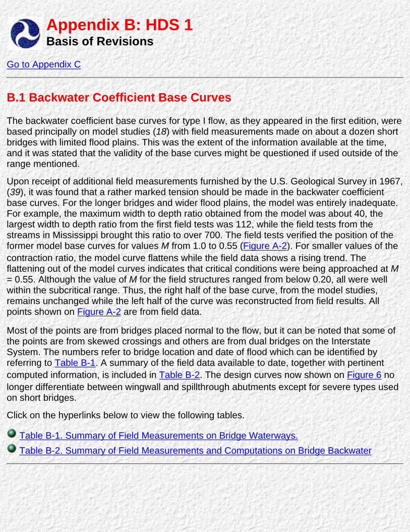
Appendix B: HDS 1Basis of Revisions

Go to Appendix C

B.1 Backwater Coefficient Base Curves

The backwater coefficient base curves for type I flow, as they appeared in the first edition, werebased principally on model studies (18) with field measurements made on about a dozen shortbridges with limited flood plains. This was the extent of the information available at the time,and it was stated that the validity of the base curves might be questioned if used outside of therange mentioned.

Upon receipt of additional field measurements furnished by the U.S. Geological Survey in 1967,(39), it was found that a rather marked tension should be made in the backwater coefficientbase curves. For the longer bridges and wider flood plains, the model was entirely inadequate.For example, the maximum width to depth ratio obtained from the model was about 40, thelargest width to depth ratio from the first field tests was 112, while the field tests from thestreams in Mississippi brought this ratio to over 700. The field tests verified the position of theformer model base curves for values M from 1.0 to 0.55 (Figure A-2). For smaller values of thecontraction ratio, the model curve flattens while the field data shows a rising trend. Theflattening out of the model curves indicates that critical conditions were being approached at M= 0.55. Although the value of M for the field structures ranged from below 0.20, all were wellwithin the subcritical range. Thus, the right half of the base curve, from the model studies,remains unchanged while the left half of the curve was reconstructed from field results. Allpoints shown on Figure A-2 are from field data.

Most of the points are from bridges placed normal to the flow, but it can be noted that some ofthe points are from skewed crossings and others are from dual bridges on the InterstateSystem. The numbers refer to bridge location and date of flood which can be identified byreferring to Table B-1. A summary of the field data available to date, together with pertinentcomputed information, is included in Table B-2. The design curves now shown on Figure 6 nolonger differentiate between wingwall and spillthrough abutments except for severe types usedon short bridges.

Click on the hyperlinks below to view the following tables.

Table B-1. Summary of Field Measurements on Bridge Waterways. Table B-2. Summary of Field Measurements and Computations on Bridge Backwater

B.2 Distance to Maximum Backwater Curves

To obtain consistency in the plotting of field data, it was advisable to draw a new set of curvesto define "Distance to Maximum Backwater". Figure 11 of the 1960 edition has been replacedby Figure 13 in this publication. The former was based entirely on model data which wasunrewarding, while Figure 13 was constructed from field data. Figure 13 is included for asecond time as Figure B-1 to show the points from which the curves were drawn. The numbersagain identify the bridge location which may be identified from Table B-1. The procedureamounted to a cut and try process along with the computations. Fortunately, there wassufficient information to define a satisfactory set of curves. (See columns 7 through 10 of TableB-2.) The principal reason for changing the parameter of the abscissa in Figure 13 and FigureB-1 to ∆h/ was to facilitate the processing of the field data which is the exact reverse of theprocedure for computing backwater.

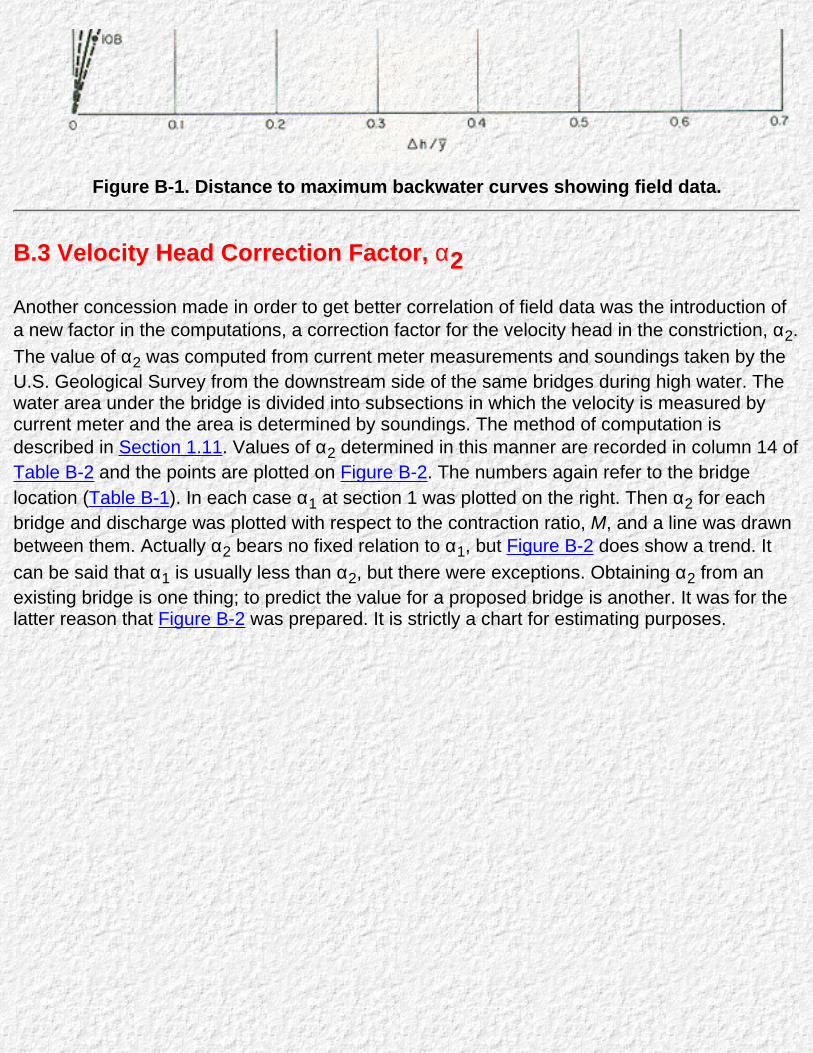
Figure B-1. Distance to maximum backwater curves showing field data.

B.3 Velocity Head Correction Factor, α2

Another concession made in order to get better correlation of field data was the introduction ofa new factor in the computations, a correction factor for the velocity head in the constriction, α2.The value of α2 was computed from current meter measurements and soundings taken by theU.S. Geological Survey from the downstream side of the same bridges during high water. Thewater area under the bridge is divided into subsections in which the velocity is measured bycurrent meter and the area is determined by soundings. The method of computation isdescribed in Section 1.11. Values of α2 determined in this manner are recorded in column 14 ofTable B-2 and the points are plotted on Figure B-2. The numbers again refer to the bridgelocation (Table B-1). In each case α1 at section 1 was plotted on the right. Then α2 for eachbridge and discharge was plotted with respect to the contraction ratio, M, and a line was drawnbetween them. Actually α2 bears no fixed relation to α1, but Figure B-2 does show a trend. Itcan be said that α1 is usually less than α2, but there were exceptions. Obtaining α2 from anexisting bridge is one thing; to predict the value for a proposed bridge is another. It was for thelatter reason that Figure B-2 was prepared. It is strictly a chart for estimating purposes.

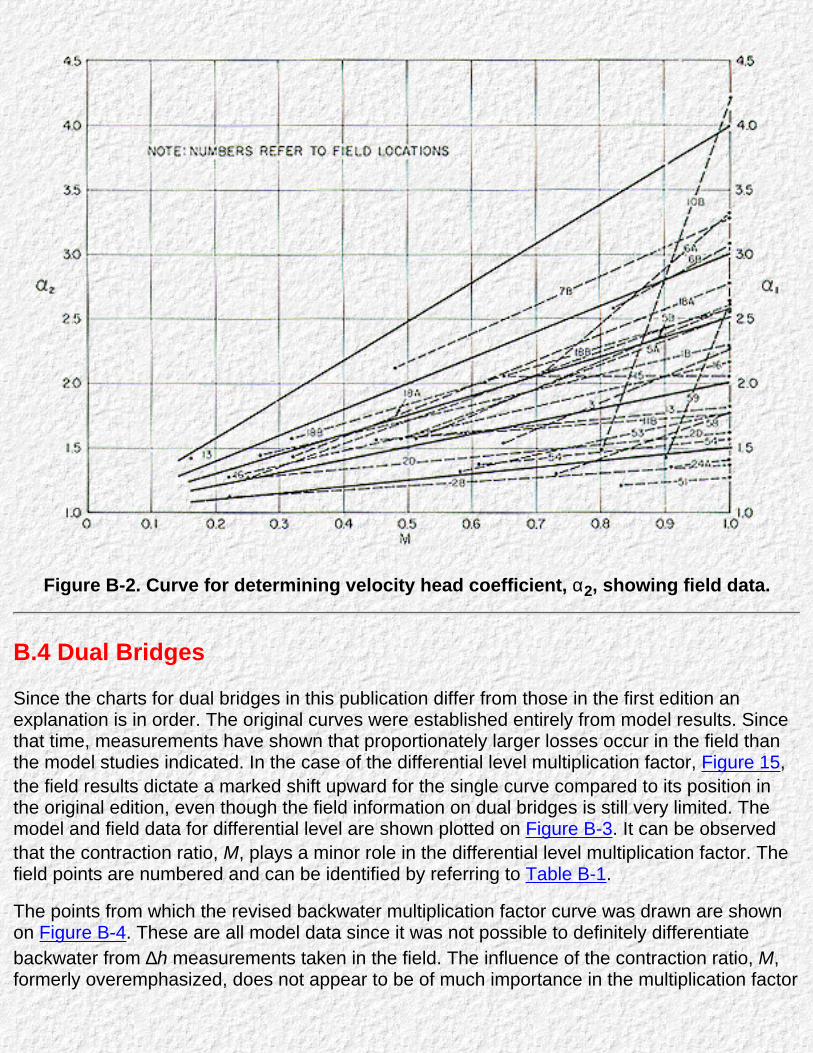
Figure B-2. Curve for determining velocity head coefficient, α2, showing field data.

B.4 Dual Bridges

Since the charts for dual bridges in this publication differ from those in the first edition anexplanation is in order. The original curves were established entirely from model results. Sincethat time, measurements have shown that proportionately larger losses occur in the field thanthe model studies indicated. In the case of the differential level multiplication factor, Figure 15,the field results dictate a marked shift upward for the single curve compared to its position inthe original edition, even though the field information on dual bridges is still very limited. Themodel and field data for differential level are shown plotted on Figure B-3. It can be observedthat the contraction ratio, M, plays a minor role in the differential level multiplication factor. Thefield points are numbered and can be identified by referring to Table B-1.

The points from which the revised backwater multiplication factor curve was drawn are shownon Figure B-4. These are all model data since it was not possible to definitely differentiatebackwater from ∆h measurements taken in the field. The influence of the contraction ratio, M,formerly overemphasized, does not appear to be of much importance in the multiplication factor

either, as Figure B-4 indicates, so M has been dropped and the original family of curves havebeen replaced by the single modified curve shown on Figure 14. The model data andcomputations from which Figure 14 and Figure 15 were prepared are recorded in Table B-3.

Figure B-3. Differential level multiplication factor for dual parallel bridges.

Figure B-4. Backwater multiplication factor for dual parallel bridges.

Click here to view Table B-3. Model Computation on Dual Bridges

Go to Appendix C

Appendix C : HDS 1Development of Chart for Determining Length of Spur Dikes

Go to Table of Contents

The information available at this time on spur dikes are plotted on Figure C-1. The field data(39) and the limited model data (19) and (25) from which the points were plotted, aresummarized in Table C-1. The information leaves much to be desired. Spur dikes in existenceappear to have been proportioned by individual judgment rather than by any definite method;some are too long while others are extremely short when compared to the lengths given byFigure C-1. The actual and computed lengths can be compared most readily by comparing thevalues of Ls in columns 18 and 19 of Table C-1.

Model testing was not only limited in range by the discharge ratio, Qf /Q100, but thereproduction of flow patterns, scour patterns, scour depths, and embankment stability was notnecessarily characteristic of the prototype structures. The model showed great variation inacceptable lengths of spur dike so, rather than plot all the model data, a representative line wasdrawn through the lot. Values for four points read from the representative line are plotted ascircles on Figure C-1 and these are also tabulated at the bottom of Table C-1. Since it was notadvisable to construct a dimensionless design chart at this time, the model results wereconverted to prototype values by the Froude Law (scale 25:1). This ratio was determined byscaling up the model flow depth of 0.40 foot to 10 feet which was the average depth of flowencountered in the field tests.

It is apparent that the design curves (Figure 30), which are based principally on the informationin Table C-1, will most likely be subject to later adjustment as additional field data are obtainedand more experience is gained. This is the first attempt at standardization of spur dike designfor bridges.

Figure C-1. Length of spur dikes.

Click here to view Table C-1. Summary of Field data and Computation on Spur Dikes.

Table C-1. Summary of Field Data and Computations on Spur DikesNo. Q

c.f.sK1 x 103 Ka x 103 Kc x

103Kb x 103 Qa

c.f.s.Qc

c.f.sQb

c.f.se =1 -

Ka/Kc

Q100 =Q/b x100c.f.s

b ft An2 ft2 =

An2/bft

Qa/Q100 Qc/Q100 Vn2 =Q/An2ft./sec

Lsexisting

ft

Ls fromFigure 30

ft.

Remarks

1 2 3 4 5 6 7 8 9 10 11 12 13 14 15 16 17 18 19 201B 14,600 1,300 190 756 354 2,150 8,480 3,970 0.748 3,000 486 2,709 5.55 0.718 2.83 5.40 26 38

2B 8,950 617 67.5 413.5 136 979 5,998 1,973 .837 2,580 347 1,671 4.82 .380 2.33 5.35 24 140

23 20

23 120

3 36,400 3,606 570 706 2,330 5,753 7,127 23,520 .196 3,480 1,044 13,315 12.75 1.66 2.08 2.73 9 44 Dual Bridges

132 56

4D 18,800 1,033 230 468 335 4,180 8,518 6,096 .505 3,880 486 4,966 10.20 1.08 2.20 3.80 0 38

90 78 Dual Bridges

5A 13,500 1,836 210 730 893 1,544 5,368 6,588 .712 2,610 519 6,427 12.40 .59 2.05 2.10 15 12

108 48

7B 3,160 515 160 109 246 982 669 1,509 .322 1,6340 236 1,756 7.45 .73 0.50 1.80 49 13

0 0

10B 5,470 296 34 23 236 629 480 4,361 .229 1,340 408 3,822 9.38 .47 0.36 1.43 127 0

0 0

11B 64,470 4,325 459 1,900 1,966 6,630 27,443 28,397 .759 5,000 1,245 12,294 9.90 1.32 5.50 5.08 0 65

114 230

13 5,430 1,590 212 1,117 261 724 3,815 891 .710 1,410 385 2,808 7.30 .51 2.71 1.93 0 0

96 56

16 4,840 467 91 274 102 943 2,840 1,057 .667 2,990 163 727 4.30 .32 0.95 6.67 0 23

52 64 Dual bridges

18A 18,000 1,479 41 765 673 499 9,310 8,191 .946 3,090 584 6,067 10.40 .16 3.01 2.97 9 0 45º skew

125 88+44 Relief bridge

20A 3,763 159 39 99 20 923 2,343 497 .605 3,330 113 804 7.16 .28 0.70 4.69 0 12 Dual bridge

163 32

24A 31,210 3,440 100 200 3,140 907 1,815 28,488 .500 4,950 630 11,644 10.50 .18 0.37 2.65 0 0

150 0

24B 10,302 1,370 90 620 660 677 4,662 4,963 .755 2,240 462 6,819 14.80 .30 2.08 1.52 0 0

70 38

30A 158,000 24,107 2,850 8,307 12,950 18,679 54,445 84,876 .657 2,870 5,512 79,400 14.40 6.52 18.95 1.99 40 140 Relief bridge

40 290

30B 16,800 1,100 47 698 355 718 10,600 5,422 .933 3,380 497 4,852 9.80 .21 3.15 3.46 18 0 Relief bridge

40 105

33G 6,136 1,600 860 560 180 3,298 2,148 690 .349 1,655 370 2,404 6.50 2.00 1.30 2.55 85 50 45º skew

0 32

36 200,000------------------------------------------- 35,800 0 164,200 1.00 6,900 2,900 43,500 15.0 5.20 0 4.60 300 200+100

0 0

37 750,000------------------------------------------- 113,500 80,000 556,500 .295 22,700 3,300 53,600 16.2 5.00 3.53 14.0 400 400

400 360

Typical Model Data Converted to 25:1 Scale101102103104

15,000-------------------------------15,000------------------------------15,000------------------------------15,000------------------------------

3,6004,8007,1209,730

0000

11,40010,200

7,8805,270

1.001.001.001.00

7,5007,5007,5007,500

200200200200

2,0002,0002,0002,000

10.010.010.010.0

.48

.64

.951.30

0000

7.507.507.507.50

38---------------50---------------75---------------100--------------

Table B-1. Summary of Field Measurements on Bridge WaterwaysNo. Location Date of

MeasurementsLength Spur

dike, feetAbutmenttype and

slope

Remarks

Left Right1B Bucantuna Creek, S.H. 18 near

Quitmann, Miss.Apr. 6, 1964 26 24 1.5:1 ST Analysis no

applicable1C -----do Apr. 7, 1964 26 24 1.5:1 ST Do.2B Long Creek, S.H. 18 near Quitmann,

Miss.Apr. 6, 1964 23 23 1.5:1 ST Do.

2D -----do Apr. 7, 1964 23 23 1.5:1 ST Do.3 Bowie Creek, I-59 near Hattisburg, Miss. Feb. 22, 1961 132 9 4:1 ST Dual Bridges Feb. 23, 1961 4D East Tallahala Creek, S.H. 258 near Bay

Springs, Miss.Apr. 6, 1964 90 0 2:1 ST Analysis not

applicable5A Tallahoma Creek, I-59 near Ellisville,

Miss.Feb. 23, 1961 15 108 3:1 ST Dual Bridges

5B -----do Apr. 8, 1964 15 108 3:1 ST Do.6A Tallahala Creek, S.H. 42 near

Runnelstown, Miss.Feb. 25, 1961 1.5:1 ST

6B -----do Apr. 9 to 10, 1964 1.5:1 ST 7A Wolf River, S.H. 26 near Poparville,

Miss.Feb. 18, 1961 2:1 ST

7B -----do Mar. 2, 1964 49 0 2:1 ST 9A Bogue Chitto, U.S.H. 84 near

Brookhave, Miss.Mar. 28, 1961 2:1 WW 30º skew

No. Location Date ofMeasurements

Length Spurdike, feet

Abutmenttype and

slope

Remarks

Left Right9B -----do Mar. 2, 1961 2:1 WW Do.10A West Hobolochitto Creek, S.H. 26 near

Poplarville, Miss.Nov. 4, 1961 2:1 ST

10B -----do Mar 2, 1964 127 0 2:1 ST 11B West Fork Tombigbee River, U.S.H. 45

near Nettletown, Miss.Apr. 12, 1962 0 114 2:1 ST

11C -----do Mar. 15, 1964 0 114 2:1 ST 12 Yockanookany River, S.H. 35 near

Kosciusko, Miss.Dec. 18, 1964 2:1 ST 27º skew

13 Black Creek, S.H. 589 near Purvis, Miss. Apr. 28, 1962 96 0 3:1 ST 15 Upper Little Creek, U.S.H. 98 near

Columbia, Miss.Apr. 28, 1962 1.5:1 ST 30º skew

16 Luke Flupper Creek, S.H. 528 near BaySprings, Miss.

Apr. 6, 1964 0 52 2:1 ST

18A Tallahala Creek, I-59 near Laurel, Miss. Feb. 23, 1961 9 125 3:1 ST (Dual Bridges) 30ºskew.

18B -----do Apr. 7, 1964 9 125 3:1 ST Do.20A Big Black River, S.H. 16 near Canton,

Miss.Dec. 19, 1961 0 163 2:1 WW Multiple Opening

22A Big Black River, I-20 near Edwars, Miss. Dec. 20, 1961 2:1 ST Dual BridgesNo. Location Date of



slope

Remarks

Left Right23 Leaf River, U.S.H. 98 near McLain, Miss. Feb. 26, 1961 2:1 ST 24A Leaf River, I-59 near Moselle, Miss. Feb. 24, 1961 150 0 2:1 ST Dual Bridges-

Multiple24B -----do. Feb. 24, 1961 0 70 2:1 ST Do.30A Pascagoula River, S.H. 26 near Merril,

MissFeb. 27, 1961 40 40 2:1 ST Multiple opening

30B -----do Feb. 27, 1961 18 40 2:1 ST Relief bridge33G Pearl River, S.H. 43 near Canton, Miss. Dec. 21, 1961 85 0 1.5:1 ST Do.34 White Sand Creek, County Highway,

near Oakvale, Miss.Mar. 29, 1961 1.5:1 ST Scour recorded

36 Susquehanna River, near Nanticoke, Pa. Apr. 1, 1960 300 2:1 ST 45º skew37 Indus River at Tarbela Dam, District

Hazara, West PakistanModel 400 2:1 ST

50 Bonnett Carre Sp. near New Orleans,La.

Feb. 28, 1937 2:1 ST

51 Short Creek near Albertsville, Ala. Nov. 28, 1948 1:1 ST 52 Bond Creek, Dunham Basin, New York Dec. 31, 1948 45º WW 53 Auglaise River, Fort Jennings, Ohio Feb. 15, 1950 45º WW No. Location Date of



slope

Remarks

Left Right54 Crooked Creek, Richmond Mo. July 6, 1951 1.5:1 ST 55 W. Br. Delaware River, Hale Eddy, N.Y. Mar. 22,1948 90º WW 56 Wild Rice Creek, Twin Valley, Minn. May 9, 1950 45º WW 57 Long Creek, Courtland, Miss. May 28, 1954 2:1 ST 58 Ottowa River, Allentown, Ohio Feb. 14, 1950 90º WW 15º skew59 Illinois Bayou, Scotsville Ark. Jan. 24, 1949 2:1 ST 60 S. Chickamauga Creek, Chickamauga,

Tenn.Mar. 29, 1948 3:1 ST 30º skew

61 Kayaderosseros Creek, West Milton,N.Y.

Dec. 31, 1948 45º WW

62 -----do Apr. 6, 1952 38º WW 8º skew63 -----do Apr. 2, 1952 38º WW 8º skew64 Schroon River, Riverbank, N.Y. Apr. 18, 1952 30º WW

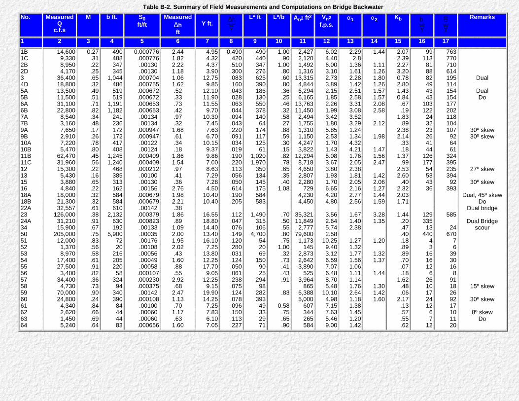
Table B-2. Summary of Field Measurements and Computations on Bridge BackwaterNo. Measured

Qc.f.s

M b ft. S0ft/ft

Measured∆hft

Y ft.

L* ft L*/b An2 ft2 Vn2f.p.s.

α1 α2 Kb Remarks

1 2 3 4 5 6 7 8 9 10 11 12 13 14 15 16 17 1B1C2B2D34D5A5B6A6B7A7B9A9B10A10B11B11C1213151618A18B22A2324A34505152535455565758596061626364

14,6009,3308,9504,170

36,40018,80013,50011,50031,10022,8008,5403,1607,6502,9107,2205,470

62,47031,96015,3005,4303,8804,840

18,00021,30032,557

126,00031,21015,900

205,00012,0001,3708,970

17,40027,5003,400

34,4004,730

70,00024,8004,3402,6201,4505,240

0.27.31.22.25.65.32.49.51.71.82.34.48.17.26.78.80.45.56.22.16.65.22.32.32.61.38.91.67.75.83.56.58.61.91.82.36.73.90.24.84.66.69.64

490488347345

1,044486519519

1,1911,182

241236172172417408

1,2451,240

468385313162584584610

2,132630192

5,9007220

21620522058

32494

34039084444483

0.000776.000776.00130 .00130

.000704

.000755

.000672

.000672

.000653

.000653.00134 .00134

.000947

.000947.00122 .00124

.000409

.000409

.000212.00100 .00130 .00156

.000679

.000679.00142

.000379

.000823.00133 .00035 .00176 .00108 .00056 .00049 .00058

.000107

.000230

.000375.00142

.000108.00100 .00060 .00060

.000656

2.441.822.221.181.061.62.52.33.73.42.97.32

1.68.61.34.18

1.861.54.97.41.36

2.761.982.21.38

1.86.89

1.092.001.952.02.43

1.60.88.55

2.92.68

2.471.13.70

1.17.63

1.60

4.954.324.373.90

12.759.85

12.1011.9011.559.70

10.307.457.636.70

10.159.379.867.008.637.297.284.50

10.4010.40

16.5518.8014.4013.4016.107.25

13.8012.2517.709.05

12.259.15

19.9014.257.257.836.107.05

0.490.420.510.300.083.160.043.028.063.044.094.043.220.091.034.019.190.220.113.056.050.614.190.205

.112

.047

.076

.149

.120

.280

.031

.124

.050

.061

.238

.075

.124

.078

.096

.150

.113

.227

49044034727662539018613055037814064

17411712561

1,0201,970

350134145175584583

1,490315106

4,700542069

1509025

29498

28239349332971

1.00.90

1.00.80.60.80.36.25.46.32.58.27.88.59.30.15.82.78.65.35.40

1.08

.70

.50

.55

.80

.751.00.32.73.41.43.91

.83

0.58.75.65.90

2,4272,1201,4921,316

13,3154,8446,2946,165

13,76311,4502,4941,7551,3101,1504,2473,822

12,2948,7184,6502,8072,280

7294,2304,450

35,32111,8492,777

79,6001,173

1452,8732,6423,890

5253,964

8656,3885,000

607344265584

6.024.406.003.102.733.892.151.852.261.993.421.805.852.531.701.435.083.673.801.931.706.654.204.80

3.562.645.742.58

10.259.403.126.597.076.488.705.48

10.104.987.157.635.469.00

2.292.8

1.361.612.281.422.512.583.313.083.523.291.241.344.324.211.762.052.381.812.052.162.772.56

1.671.402.38

1.271.321.771.561.061.111.141.762.641.181.381.451.201.42

1.44

1.111.261.801.261.571.572.082.58

2.12

1.98

1.471.562.47

1.422.061.271.441.59

3.281.35

1.20

1.321.37

1.44

1.301.421.60

2.072.392.273.200.782.801.430.84.67.19

1.83.89

2.382.14.33.18

1.37.99

2.532.60.40

2.322.031.71

1.44.20.47.40.18.89.89.70.07.18

1.62.48.06

2.17.13.57.55.62

99113818882494343

103122243223264144

12617754534336

12933513

44043

1616126

261017241267

12

763770710614195114154154177202118104107926461

32439523539492

393

585

24670

76

3930168

9118269217101120

Dual

DualDo

30º skew30º skew

27º skew

30º skew

Dual, 45º skewDo

Dual bridge

Dual Bridgescour

15º skew

30º skew

8º skewDo

Table B-3. Model Computations on Dual Bridges

RunNo. b ft. Q

c.f.s. Yn ft. hd*ft. M=b/B

An2=hn· b

ft.

Vn2 =Q/An2f.p.s.

ft.

Kb

h1* =

ft.

hD ft.h3B* =hn - hD

ft.

hd*+ h3B*ft

h1* +h3*

Abutmenttype

(1) (2) (3) (4) (5) (6) (7) (8) (9) (10) (11) (12) (13) (14) (15) (16) (17) (18) (19) (20)809816R833834839R840842R8479609671,329303132333435363738391,340895R902903908909915916RR

4.464.422.422.422.422.422.422.422.422.422.853.874.875.902.853.854.875.872.833.854.875.874.422.422.422.422.422.424.42

2.50|||||||||

3.00|||||||||||

5.00||||||

0.333|||||||||

.370|||||||||||

.484||||||

0.051.555.195.208.203.217.222.220.211.215

0.170.081.039.016.174.089.043.018.190.094.046.018.089.342.367.351.361.372.095

0.565.559.306

|||||||

.361

.490

.616

.747

.361

.487

.616

.743

.361

.487

.616

.743

.559.306.306.306.306.306.559

4.3311.004.33

||

11.00||||

4.33|||

7.67|||

11.0|||

4.33|

7.674.33

11.00||

1.4851.4720.806

|||||||

1.0551.4321.8022.1831.0551.4251.8022.1721.0551.4251.8022.1722.1391.1711.1711.1711.1711.1712.139

1.6841.6983.102

|||||||

2.8442.0951.6651.3742.8442.1051.6651.3812.8442.1051.6651.3812.3384.2704.2704.2704.2704.2702.338

0.042.045.149

|||||||

.125

.068

.043

.029

.125

.069

.043

.029

.125

.069

.043

.029

.081

.283

.283

.283

.283

.283

.085

0.82.82.95

|||||||

.95

.88

.68

.40

.95

.88

.68

.40

.95

.88

.68

.40

.75

.90

.90

.90

.90

.90

.75

0.035.037.142.142.142.142.142.142.142.142.119.060.029.012.119.060.029.012.119.060.029.012.061.255.254.255.255.255.064

1.4521.4861.3731.4651.4301.5281.5631.5491.4861.5141.4291.3501.3361.3681.4621.4711.4731.5251.5931.5541.5751.5251.4641.3421.4401.3781.4171.4601.491

0.308--

.298

.290

.285

.295

.284

.298

.295--

.342

.337

.345

.353

.339

.337

.345

.352

.330

.337

.343

.353

.438

.394

.410

.391

.411

.406

.429

0.25--

.035

.043

.048

.038

.049

.035

.038--

.028

.033

.075

.017

.031

.033

.025

.018

.040

.033

.027

.017

.046

.090

.074

.093

.073

.078

.055

0.076--

.230

.251

.251

.255

.271

.255

.249--

.198

.114

.064

.033

.205

.122

.068

.036

.230

.127

.076

.036

.135

.412

.441

.444

.434

.430

.150

0.63--

.83

.83

.83

.83

.83

.83

.83--

.79

.69

.59

.46

.79

.70

.59

.46

.79

.71

.58

.46

.64

.83

.83

.83

.83

.83

.64

0.055--

.171

.171

.171

.171

.171

.171

.171--

.151

.086

.495

.254

.151

.086

.049

.026

.151

.085

.049

.026

.095

.307

.307

.307

.307

.307

.099

1.369--

1.3451.4681.4681.4911.5851.4911.456

--1.3111.3111.2931.2991.3581.4121.3731.4011.5231.4911.5351.3601.4211.3421.4461.4461.4731.4011.508

WW45º

1,3171819202122R23242526R28

2.8863.8664.8865.8862.8463.8664.8565.8762.8763.8865.886

5.00||||||||||

.484||||||||||

.265

.140

.070

.030

.266

.142

.069

.030

.246

.129

.027

.363

.489

.618

.745

.360

.489

.615

.744

.364

.492

.745

||||

7.67|||

4.33

1.3871.8712.3652.8491.3771.8712.3502.8441.3921.8802.849

3.6052.6722.1141.7553.6312.6722.1281.7583.5922.6601.755

.202

.111

.069

.048

.205

.111

.070

.048

.200

.110

.048

.87

.85

.69

.40

.87

.85

.68

.40

.90

.85

.40

.175

.094

.048

.019

.178

.094

.048

.019

.180

.093

.019

1.5091.4861.4601.5711.4941.5071.4431.5671.3641.3811.414

.424

.440

.456

.459

.417

.440

.664

.460

.413

.432

.461

.060

.044

.028

.025

.067

.044

.020

.024

.071

.052

.023

.325

.184

.098

.055

.333

.186

.097

.054

.317

.181

.050

.79

.70

.59

.46

.79

.70

.60

.46

.79

.69

.46

.222

.135

.081

.041

.225

.135

.080

.042

.228

.135

.041

1.4641.3631.2101.3301.4801.3781.2171.2901.3901.3411.205

ST

Table A-1. Critical Flow Through Bridge Constriction (Type II and III Flow) Model Data and ComputationsRunNo.

B.ft.

bft.

Qc.f.s.

M =b/B

Ynft.

h1*ft

Yn + h1*ft

Y1cft

Y2cft

Y3ft

A1 = B(Yn + h1*)ft.2

V1 = Q/A1f.p.s.

A2c = b x Y2cft.2

V2c = Q/A2cf.p.s

V22c/2gft.

Yn+h1*- Y2cft

Yn + h1*-Y2cV22c/2g

Cb So Abutmenttype

FlowType

1 2 3 4 5 6 7 8 9 10 11 12 13 14 15 16 17 18 19 20 21 22 23357267266456305229261602262858601755872304228

1,2281,3021,2691,307

132029192130

823927670281557558109

1,3551,161R

24322316

445125123666589

1,061563107

7.90

4.00

7.90

4.00

7.90

2.00

2.983.00

2.812.832.832.841.50

2.00

2.4162.4162.442.452.462.462.502.852.911.581.9842.082.352.322.472.4962.652.7952.8772.9172.945

2.502.913.955.00

5.752.505.00

3.005.003.005.001.981.06.661.062.251.572.505.002.505.005.005.005.303.003.002.251.572.251.072.502.452.682.505.005.005.005.30

0.253

.377

.380

.356

.358

.358

.359

.375

.500

.306

.306

.309

.310

.311

.311

.316

.361

.368

.395

.496

.520

.588

.294

.313

.316

.335

.354

.364

.369

.373

0.333.352.418.484

.416

.523

.333

.416

.484

.360

.484

.360

.484

.446

.232

.202

.232

.382

.318

.333

.484

.333

.484

.484

.484

.497

.360

.360

.386

.322

.386

.233

.333

.314

.331

.333

.416

.484

.484

.497

0.282.335.417.476.484.478.481.527.573.159.318.266.274.274.273.175.261.184.265.146.155.086.086.150.098.176.305.181.310.318.313.297.147.141.227.103.135.047.201.190.198.152.307.235.240.223

0.615.687.835.960.968.962.965.943

1.096.492.734.750.758.758.757.535.745.544.749.592.387.288.318.532.416.509.789.514.794.802.797.794.507.501.613.425.521.280.534.504.529.485.723.719.724.720

0.146.162.198.231.231.231.231.231.254.146.232.232.232.232.232.165.232.165.232.197.130.094.130.214.169.146.232.146.232.232.232.241.165.165.214.169.214.131.146.144.153.146.232.232.232.241

0.364.404.495.579.579.579.579.579.636.280.442.442.442.442.442.329.461.327.459.380.250.182.206.340.267.322.511.319.506.505.505.519.325.321.399.269.332.186.331.312.329.302.464.455.451.466

0.282.295.341.409.377.386.391.280.428.276.319.404.414.402.407.304.389.311.405.381.159.179.199.295.252.287.287.286.404.408.409.417.319.321.341.266.327.185.292.253.287.296.321.414.423.427

4.8595.4276.5977.5847.6477.6007.6247.4508.6583.8875.7995.9255.9885.9885.9804.2275.8864.2985.9172.3601.5481.1521.2722.1281.6644.0216.2334.0616.2706.3366.2966.2734.0053.9582.4521.7002.0841.1204.2193.9824.1793.8325.7125.6805.7205.688

0.555.536.599.659.654.658.656.671.664.643.862.844.835.835.836.710.849.698.845.838.685.573.833

1.057.944.622.802.616.800.789.794.845.749.758.918.924

1.080.955.593.615.614.652.875.880.874.932

0.728.808.990

1.158

1.272.834

1.326

.9241.305.925

1.303.570.375.273.412.680.534.778

1.235.778

1.2401.2421.2421.298.926.934.630.534.691.432.768.771.821.800

1.2971.3091.3161.372

3.4343.6013.9904.318

4.5202.9983.771

3.2483.8313.2433.8373.4742.8272.4182.5733.3092.9403.2134.0493.2134.0324.0264.0264.0833.2403.2123.5712.9403.2562.4773.2553.1783.2643.1253.8553.8203.7993.863

0.182.202.248.264

.318

.140

.221

.164

.228

.163

.229

.187

.124

.091

.103

.170

.134

.160

.255

.160

.253

.253

.253

.259

.163

.160

.198

.134

.165

.096

.165

.157

.165

.152

.232

.227

.225

.232

0.251.283.340.381.389.383.386.364.460.212.292.308.316.316.315.206.284.217.290.212.137.106.112.192.148.187.278.195.288.297.292.275.182.180.214.156.189.094.203.192.200.183.259.264.273.254

1.3791.4011.3711.4431.4731.4511.4621.3791.4471.5171.3211.3941.4301.4301.4251.2561.2461.3311.2661.1351.1051.1651.0921.0871.1041.1691.0901.2191.1401.1741.1541.0621.1171.1251.0811.1641.145.9791.2301.2231.2121.2041.1161.1631.2131.095

0.022.022.023.023.023.023.023.024.022.046.052.050.049.049.049.048.040.046.048.058.058.056.105.102.103.037.039.037.035.038.039.043.053.056.066.099.110.149.033.037.039.060.052.053.053.058

0.401.432.394.360.396.474.485.403.469.560.373.444.479.479.474.304.286.377.314.193.169.221.197.189.207.206.129.250.175.217.193.105.170.181.147.263.255.128.263.268.251.264.168.216.266.153

0.0012

.0020

.0012

.0036

.0024

.0036

.0024

.0024

.0012

.0024

.0024

.0012

.0036

.0012

VB

VWVW

90o WW

45o WW

ST

BBBBBBBBBABAAAAAAAAABAAAAABABBBBAABAAAAAAABAAA

List of Tables for HDS 1-Hydraulics of Bridge Waterways


Table 1. Manning's roughness coefficient for natural stream channels1.

Table 2. Example 1: Sample Computations S0 = 0.0049

Table 3. Example 4: Computer sheet for one stage and one bridge length.

Table 4. Example 4: Summary of computer calculations.

Table 5. Example 6: Sample computations-properties of natural stream. [Q = 9,460 c.f.s.; Measured S0 =0.00208; Normal Stage Elevation = 23.9 ft]

Table 6. Example 11: Computer sheet.

Table A-1. Critical Flow Through Bridge Constriction (Type II and III Flow) Model Data and Computations

Table B-1. Summary of Field Measurements on Bridge Waterways

Table B-2. Summary of Field Measurements and Computations on Bridge Backwater

Table B-3. Model Computations on Dual Bridges

Table C-1. Summary of Field Data and Computations on Spur Dikes


List of Equations for HDS 1-Hydraulics of Bridge Waterways


Equation 1

Equation 2

Equation 3a

Equation 3b

Equation 4

Equation 4a

Equation 4b

Equation 5

Equation 6

Equation 7

Equation 8

Equation 9

Equation 10

Equation 11

Equation 12

Equation 13

Equation 14

Equation 15

Equation 16

Equation 17

Equation 18

Equation 19

Equation 20

Equation 21

Equation 22

Equation 23

Equation 24

Equation 25

Equation 26

Equation 27

Equation 28

Equation 29

Equation 30

Equation 31

Equation 32

Equation 33


Preface : HDS 1


The design Information in the first edition of "Hydraulic of Bridge Waterways," published in1960, was based principally on the results of hydraulic model studies and was definitely limitedin its range of application. Over the intervening 10 years, the U.S. Geological Survey has takenmeasurements and collected field data on the hydraulics of bridges during floods. Uponexamination of the field data, it was deemed advisable to reevaluate the model results todetermine the actual limits of application and then utilize the field data to complete the designcurves.

This edition thus contains revisions to some of the design curves. A considerable amount ofnew material has been added such as chapters on partially inundated superstructures, theproportioning of spur dikes at bridge abutments, and supercritical flow under a bridge, togetherwith examples. An appendix has also been included to show how and why changes were madeto some of the former design curves. The field results have added considerably to the reliabilityof the information contained herein.

Mr. Lester A. Herr, Chief of the Hydraulics Branch, Bridge Division, requested and supervisedthe preparation of this revised edition of the "Hydraulics of Bridge Waterways." Many thanks goto Mr. Herr and Mr. J. K. Searcy of his staff for their time and helpful suggestions in thetechnical editing of the present edition. The research program on bridge waterways, which wasthe basis of the first edition, was directed by Carl F. Izzard, then chief of the HydraulicsResearch Division of the Federal Highway Administration. The writer, who served as projectsupervisor, is greatly indebted to Mr. Izzard for his gifted guidance and timely suggestions.


Forward : HDS 1


Bridges across waterways are grade separation structures like those built to carry vehiculartraffic over or under other highways. The important difference is that the hydraulic traffic cannotbe controlled by passing statutes or erecting signs. However, the action of a stream can bepredicted and controlled to an extent if flood data are secured for some distance both upstreamand downstream from the bridge crossing, and the data are analyzed by an engineer trained inhydraulics, hydrology, and river behavior.

An important consideration in the hydraulic analysis of a proposed bridge crossing is theamount of backwater produced by constricting the flow of a stream with the highway crossing. Backwater, in itself, can cause flooding upstream from the highway crossing. In addition, theincreased velocity of the stream through the bridge opening and the turbulence produced byoverbank flow returning to the channel can produce scour sufficient to endanger the bridgestructure. The importance of backwater in the analysis of bridge waterways led to the researchwhich was the basis for the first edition of "Hydraulic of Bridge Waterways." This publication iswidely used by highway bridge designers and a computer program has been written to moreeasily compute bridge backwater.

Field measurements taken by U.S. Geological Survey on streams with wide flood plains andbridges that impose a severe contraction on the flow area showed that the backwater in someinstances was higher than indicated in the previous publication, which was based primarily onmodel studies. The field data warranted a revision of the first edition. This second editioncontains revisions of the first edition plus much new material, particularly on spur dikes, bridgesuperstructure partially inundated, and flow which passes through critical depth in theconstriction.

We were fortunate to obtain Mr. Joseph N. Bradley, the author of the first edition, as aconsultant to prepare this second edition. We also appreciated the field measurement datasupplied by the U.S. Geological Survey and used to check and supplement the model datawhich was the principal basis of the first edition.

Lester A. Herr, Chief, Hydraulics Branch,

Bridge Division, Office of Engineering and Operations.


References

1. ASCE. "Economics of Self-protection of Highways Against Flood Damage,"by J.C. Young, Journal of Highway Division, HW 3, October 1956, Paper 1075.

2. ASCE, "Effect of Spur Dikes on Flow Through Contractions,"by E.R. Headman, Journal of Hydraulics Division, Vol. 91,HY-4, July 1965, Paper 4412.

3. ASCE, Journal of Hydraulics Division, Vol. 92, HY-2, March 1996, p.430.(Discussion of ref.2 by L.A.Herr)

4. ASCE, "Systematic Changes in the Beds of Alluvial Rivers,"by W.C. Carey and M.D. Keller, Journal of Hydraulics Division,Vol. 83, HY-4, August 1957, Paper 1331.

5. ASCE Trans., "Flood Erosion Protection for Highway Fills,"by C.P. Posey, Vol. 122, 1957, p. 531.

6. ASCE Trans. Vol. 122, 1957, p. 544(Discussion of Ref. 5 by C.F. Izzard and J.N. Bradley.)

7. ASCE Trans. Vol. 122, 1957, p.548.(Discussion of ref. 5 by C.E. Kindsvater)

8. ASCE Trans., "Tranquil Flow Through Open Channel Constrictions,"by C.E. Kindsvater and R.W. Carter, Vol. 120, 1955, p. 955.

9. ASCE Trans., "Backwater Effects of Open-Channel Constrictions,"by H.J. Tracy and R.W. Carter, Vol. 120, 1955, p. 993.

10. Bradley, J. N., ''The Use of Backwater in the Design of Bridge Waterways,"Public Roads, Vol. 30, No. 10, October 1959, p. 221.

11. Bradley, J. N., ''Use of Backwater in Designing Bridge Waterways,Highway Research Board Bulletin 242, Washington, D,C,, 1960, p. 57.

12. Bureau of Public Roads, Estimating Flood Discharges in the Piedmont Plateau,by W. D. Potter, Hydraulic Engineering Circular No. 2, Washington, D.C.,November 1960, 21 pp.

13. Bureau of Public Roads, Hydraulics of Bridge Waterways,by K. H. Welty, M. L. Corry, and J. L. Morris, Electronic Computer Program HY-4-69,Washington, D.C., 1969.

14. Bureau of Public Roads, Hydraulic Charts for the Selection of Highway Culverts,by L. A. Herr, Hydraulic Engineering Circular No. 5, Washington, D.C.,U.S. Government Printing Office, December 1965, 54 pp.

15. Bureau of Public Roads, Peak Rates of Runoff From Small Watersheds,

by W. D. Potter, Hydraulic Design Series No. 2, Washington, D.C.,U.S. Government Printing Office, April 1961, 35 pp.

16. Bureau of Public Roads, Use of Riprap for Bank Protection,by J. K. Searcy, Hydraulic Engineering Circular No. 11, Washington, D.C.,U.S. Government Printing Office, June 1967, 43 pp.

17. Chow, Ven Te, Open Channel Hydraulics,New York, McGraw-Hill, 1959, p. 226.

18. Colorado State University, Civil Engineering Section, Backwater Effectsof Piers and Abutments, by H. K. Liu, J. N. Bradley, and E. J. Plate,Report CER57HKL10 October 1957. 364 pp.

19. Colorado State University, Civil Engineering Section,Hydraulic Model Study of Spur Dikes for Highway Bridge Openings,by S. S. Karaki, Report CER59SSK36, September 1959, 47 pp.

20. Colorado State University, Civil Engineering Section,Mechanics of Local Scour, Part II, Bibliography,by S. S. Karaki and R. M. Haynie, CER63SSK46, Fort Collins, Colo.,November 1963, 51 pp.

21. Colorado State University, Civil Engineering Dept., Engineering Research Center,Mechanics of Local Scour, by H. W. Shen, V. R. Schneider, and S. S. Karaki,CER66HWS22, Fort Collins, Colo., June 1966, 58 pp.

22. Corry, M. L. and W. Sanger, ''Ultrasonic Instrument for Determining Scour at Bridge Piers,Public Roads, Vol. 35, No. 4, October 1968, p.91.

23. Iowa Highway Research Board, Scour Around Bridge Piers and Abutments,by E. M. Laursen, and A. Toch, Bulletin 4, May 1956, 60 pp.

24. Iowa Highway Research Board, Scour at Bridge Crossings,by E. M. Laursen, Bulletin 8, August 1958, 53 pp.

25. Karaki, S. S. "Laboratory Study of Spur Dikes for Highway Bridge Protection,Highway Research Board Bulletin 286, Washington, D.C., 1961, p.31.

26. Kindsvater, C. E., R. W. Carter, and H. J. Tracy,Computation of Peak Discharge at Contractions, U.S. Geological Survey Circular 284,Washington, D.C., 1053, 35 PP.

27. Lehigh University Institute of Research, Spur Dikes Prevent Scour at Bridge Abutments,by J. B. Herbich, Fritz Engineering Laboratory Report 280.20, Bethlehem, Pa.,December 1966.

28. National Hydraulic Laboratory, Etude Des Affouillements Autour Des Piles De Ponts,(Study of scour around bridge piers), Series A, Chatou, France, October 1956.

29. Sanden, E. J., Scour at Bridge Piers and Erosion of River Banks,

Department of Highways, Province of Alberta, Canada, 3 October 1960.30. Schneible, D. E., Field Observations on Performance of Spur Dikes at Bridges,

Philadelphia, Pa., 17n21 October 1966.(Paper presented at ASCE Transportation Engineering Conference.)

31. State University of Iowa, Field Verification of Model Tests on FlowThrough Highway Bridges and Culverts, by C. F. Izzard and J. N. Bradley,Studies in Engineering, Bulletin 39, June 1958, p. 225.(Proceedings 7th Hydraulics Conference.)

32. Tainish, J. Investigation of Forces on Submerged Bridge Beams, Report No. 108,New South Wales, Australia, March 1965.

33. U.S. Department of Agriculture, Bridge Piers as Channel Obstructions,by D. L. Yarnell, Technical Bulletin No. 442, Washington, D.C.,U.S. Government Printing Office, November 1934, 52 pp.

34. U.S. Department of Agriculture, Flow of Water in Drainage Channels,by C. E. Ramser, Technical Bulletin No. 129, Washington, D.C.,U.S. Government Printing Office, November 1929, 102 pp.

35. U.S. Department of Agriculture, Flow of Water in Channels Protectedby Vegetative Linings, by W. O. Ree and V. J. Palmer, Technical Bulletin No. 967,Washington, D.C., U.S. Government Printing Office, February 1949, 115pp.

36. U.S. Department of Agriculture, Pile Trestles as Channel Obstructions,by D. L. Yarnell, Technical Bulletin, No. 429, Washington, D.C.,U.S. Government Printing Office, July 1934.

37. U.S. Geological Survey, Discharge Characteristics of Embankment-Shaped Weirs,by C. E. Kindsvater, Water Supply Paper 1617-A, Washington, D.C.,U.S. Government Printing Office, 1964, 114 pp.

38. U.S. Geological Survey, Flow Through Openings in Width Constrictions,by J. Davidian, P. H. Carrigan Jr., and J. Shen, Water Supply Paper 1369-D,Washington, D,C., U.S. Government printing 1962, 32 pp.

39. U.S. Geological Survey, ''Hydraulic Performance of Bridges in the State ofMississippi" by B. L. Neely, Jr., Jackson, Miss., 30 June 1966.(Unpublished report.)

40. U.S. Geological Survey, Measurement of Peak Discharge at WidthConstrictions by Indirect Methods, by H. F. Matthai, Techniques ofWater Resources Investigations, Book 3, Chapter A4,Washington, D.C., U.S. Government Printing Office, 1967, 44 pp.

41. U.S. Geological Survey, Roughness Characteristics of Natural Channels,

by H. H. Barnes, Jr., Water Supply Paper 1849, Washington, D.C.,U.S. Government Printing Office, 1967, 213 pp.

42. Water and Power Development Authority, Hydraulic Model Studies,Tarbela Dam Project, Part II, Lahore, West Pakistan, October 1965.

43. Yarnell, D. L., and F. A. Nagler, ''Flow of Water Over Railway andHighway Embankments, Public Roads, Vol. 11, No. 2,April 1930, p. 30.

Hydraulics of Bridge Waterways

Documents

Transcript of Hydraulics of Bridge Waterways