Waterways, Wetlands and Drainage Guide - Part B: … · Waterways. Wetlands and ... scour...

22-1

Hydraulics

Page

22.1 Introduction 22-3

22.2 Uniform Flow Resistance Formulae 22-3 -~---~~---"----

22.3 Non Uniform Flow 22-6 -----"-

22.4 Determination of Water Surface Profiles 22-7

22.5 Outfall Water Levels 22-9

22.6 Afflux at Bridges and Other Structures 22-10

22.7 Bed Shear Stress and the Stable Bed 22-10

22.8 Riffle, Run, Pool Design 22-12

22.9 Hydraulic Design of Culverts and Pipes 22-12

22.10 Sumps - Collection of Water from Side 22-15 Channels

22.11 Weirs and Free Overfalls 22-16

22.12 References 22-17

Waterways. Wetlands and Drainage Guide-Ko Te Anga Whakaora rna Ngo Arawoi Repo • Part B: Design Christchurch City Council • February 2003

22-2 Chapter 22: Hydraulics

Part B: Design February 2003

Waterways , Wetlands and Drainage Guide - Ko Te Anga Whakaora rna Ngo Arawai Repa Christchurch City Council

22.1 Introduction

Designers are referred to a standard hydraulics textbook for procedures by which flow depth, velocity, and energy state can be analysed. Useful books are Pilgrim (1987), Henderson (1966), French (1985), Chow (1959), Brater and King (1976).

Some specific aspects of hydraulic design such as Manning's roughness coefficient, outfall water levels, scour velocities, and the hydraulics of structures such as bridges, sumps, and weirs are described here. Refer to a hydraulic textbook for further information.

22.2 Uniform Flow Resistance Formulae

Over the years, various expressions have been developed to predict velocity and depth of steady unifonn flow in a conduit under given conditions. The most widely used formulae are the DarcyWeisbach Formula and the Manning Formula. Both of these formulas involve empirically determined roughness parameters.

22.2. I The Darcy-Weisbach Formula

The Darcy-Weisbach Formula is commonly applied in the calculation of head losses in closed conduits of circular cross-section based on friction factor, velocity, length, and diameter. The friction factor has been further related to surface roughness and Reynolds Number via the empirical Colebrook-White formula developed from pipe experiments. The Pipe Flow Nomograph (Appendix 11) is based on a similar empirical relationship.

22.2.2 The Manning Formula

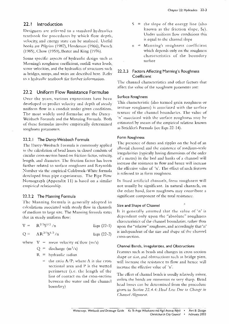
The Manning formula is generally adopted in calculations associated with steady flow in channels of medium to large size. The Manning formula states that in steady uniform flow:

V=

Q=

where V

Q

R

Eqn (22-1)

Eqn (22-2)

mean velocity of flow (m/s)

discharge (m3/s)

hydraulic radius

the ratio AlP; where A is the cross sectional area and P is the wetted perimeter (i.e. the length of the line of contact on the cross-section between the water and the channel boundary)

22.2.3

Chapter 22: Hydraulics 22-3

S the slope of the energy line (also known as the friction slope, Sf). Under uniform flow conditions this is equal to the channel slope

n Manning's roughness coefficient which depends only on the roughness characteristics of the boundary surface

Factors Affecting Manning's Roughness Coefficient

The channel characteristics and other factors that affect the value of the roughness parameter are:

Surface Roughness

This characteristic (also termed grain roughness or texture roughness) is associated with the surface texture of the channel boundaries. The value of 'n' associated with the surface roughness may be estimated by means of the empirical relation known as Strickler's Formula (see Eqn 22-14).

Form Roughness

The presence of dunes and ripples on the bed of an alluvial channel and the existence of medium-scale irregularities (typically having dimensions of the order of a metre) in the bed and banks of a channel will increase the resistance to flow and hence will increase the effective value of 'n'. The effect of such features is referred to as form roughness.

In lined artificial channels, form roughness will not usually be significant. In natural channels, on the other hand, fonn roughness may contribute a significant component of the total resistance.

Size and Shape of Channel

It is generally assumed that the value of 'n' is dependent only upon the "absolute" roughness characteristics of the channel boundaries, rather than upon the "relative" roughness, and accordingly that 'n' is independent of the size and shape of the channel cross-section.

Channel Bends, Irregularities, and Obstructions

Features such as bends and changes in cross-section shape or size, and obstructions such as bridge piers, will increase the resistance to flow and hence will increase the effective value of 'n'.

The effect of channel bends is usually relatively minor, unless the bends are numerous or very sharp. Bend head losses can be determined from the procedure given in Section 22.4.4: Head Loss Due to Challge ill Chal1l1el AI~!?ll1l/ellt.

Waterways. Wetlands and Drainage Guide-Ko Te Anga Whakaora ma Ngo Arawai Repa • Part B: Design February 2003 Christchurch City Council •


Gradual variations in the channel cross-section have relatively little effect; abrupt variations, particularly abrupt expansions, may have a significant effect.

Vegetation

The effect of vegetation on the flow resistance can be very significant, particularly in the case of small channels and overbank flow areas or flood plains. The effect of vegetation can be complex and variable -for example, small shrubs and grasses, which at low discharges offer significant resistance to the flow, may be bent over or flattened by higher flows, with a consequent decrease in the resistance offered by the vegetation. Seasonal variations and long-term change in vegetation may require consideration, and it may be necessary to take into account the extent and frequency of maintenance operations.

In general, the effects of vegetation on flow resistance will tend to be strongly dependent upon the water depth or stage.

The effects of vegetation on flow resistance are discussed by Chow (1959) and Henderson (1966), and illustrated in the table of Manning's 'n' values listed in Table 22-1 (opposite page).

Stage

In a given unlined channel, the value of'n' is likely to be relatively high at low stages, when much of the flow boundary will consist of the relatively coarse material characteristically found in the channel bed. At very high stages, the resistance to flow is likely to be increased as a result of the flow coming in contact with vegetation and other obstructions, and the value of'n' is again likely to be relatively high.

In a given channel reach, a minimUlH value of'n' will usually occur at a stage below or approaching bankfull condition. The relation between the stage and the value of'n' in a channel reach will depend upon the way in which the boundary roughness varies from point to point on the channel perimeter.

In a lined channel, the value of 'n' is less likely to be dependent upon the stage, as the roughness characteristics of the channel boundaries are more likely to be uniform.

Figure 22-/: Channel of composite roughness.

22.2.4 Estimation of Manning's Roughness

Coefficient

Channel of Single Roughness

The estimation of the value of'n' for a given flow in a given channel reach involves a level of engineering judgement. The factors that affect the value of the roughness parameter, and which should thus be borne in mind when estimating the value of 'n' for a given reach, have been outlined in ScctiOl1 22.2.3: Factors ~[rcctillg NlallllillJ!.'s ROllghlless Co~[ficiC/1t. The resources and procedures that are available to assist the investigator include:

Tables:

Table 22-1 provides a range of Manning's 'n' values. Further values can be found in tables presented by Chow (1959), Henderson (1966) and French (1985). Caution is advised, as in most cases the extent to which the reliability of the tabulated values has been established is not explicitly stated.

Photographs:

Photographs of channel reaches of known 'n' values are potentially of assistance in estimating the value of 'n' for a different reach having recognisably similar characteristics.

Chow (1959) has presented 24 black and white photographs of channel reaches with 'n' values ranging from 0.012-0.150. Barnes (1967) has presented approximately 100 colour photos from 50 channels with 'n' values ranging from 0.024-0.075. Hicks and Mason (1991) present a comprehensive set of photos and values.

Channel of Composite Roughness

In many cases, the boundary roughness varies from point to point at a given channel cross-section. For example, bed roughness may be recognisably different from the roughness of the channel banks.

With reference to Figure 22-1, the total wetted perimeter (P) is imagined to be divided into N segments, identified as P l , P2 ... PN. A particular value of the roughness parameter is associated with each segment, the respective values of the roughness

parameter being n1, n2 ... nN'

An estimate of 'n' can be obtained frOtH the following expresslOn:

n= I; ( Pi 1\ 15) y;

P Eqn (22-3)

where n the roughness parameter for the crosssection as a whole

Part B: DeSign February 2003

• Waterways. Wetlands and Drainage Guide-Ko Te Anga Whakaora mo Ngo Arawai Repo • Christchurch City Council

Chapte r 22: Hydrau lics 22-5

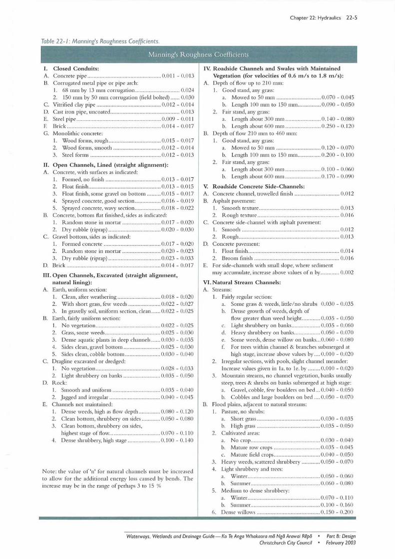
Table 22- 1: Manning's Roughness Coeffi cients.

Manning's Roughness Coefficients

I. Closed Conduits: A. Concrete pipe ....... ........................................ 0.011 - 0.013 B. Corruga ted metal pipe or pipe arch:

1. 68 ml11 by 13 nUll corrugation ............ .. ............... 0.024 2. 150 mm by 50 nUll corrugation (field bolted) ...... 0.030

C. Vitrified clay pipe .. .... ........ .. .... .... .. .. .... .... ...... 0.012 - 0.014 D. Cast iron pipe, uncoa ted ...... ..... .. ... ...... .. .. .... .......... .. ... 0.0 13 E. Steel pipe .................................... .. .. .. .. ........... 0.009 - 0.0 11 E Brick .......................................... .. ................. 0.0 14 - 0.017 G. Monolithic concrete:

1. Wood forms, rough .............. ...... ...... .. ...... 0.015 - 0.017 2. Wood for ms, smooth .......... .... .. .. ............. 0.012 - 0.014 3. Steel forms .............. ...... .. .. ...... .. .......... .. .. 0.012 - 0.013

II. Open Channels, Lined (straight alignment): A. Concrete, with surfaces as indicated:

1. Formed, no finish .......... .. ........ ........ ........ 0.0 13 - 0.017 2. Float finish ...... .... .. ...... .. .. .. .... .. ........ .... .. ... 0.0 13 - 0.Ql5 3. Float finish , some gravel on bottom .... .. ... 0.015 - 0.017 4. Sprayed concrete, good section .... .. .. .. .... ... 0.0 16 - 0.019 5. Sprayed concrete, wavy section .... .. ...... .. ... 0.018 - 0.022

B. Concrete, bottom flat finished, sides as indicated: 1. Random stone in mortar .... ...... ........ .. .... . 0.017 - 0.020 2. Dry rubble (r iprap) .................................. 0.020 - 0.030

C. Gravel bottom, sides as indicated: 1. Formed concrete ..................................... 0.0 17 - 0.020 2. Random stone in mortar ......................... 0.020 - 0.023 3. Dry rubble (rip rap) .................................. 0.023 - 0.033

D. Brick ............................................................. 0.014 - 0.0 17

III. Open Channels, Excavated (straight alignment, natural lining):

A. Earth, uniform section: 1. C lean, after weathering ............. ...... ........ 0.018 - 0.020 2. With short grass, few weeds .......... .. .... .. ... 0.022 - 0.027 3. [n gravelly soil , uniform section, clean ...... 0.022 - 0.025

B. Earth, f.l irly uni forl11 section: 1. No vegetation ...... ........ ...... .. ... ....... .... .... .. 0.022 - 0.025 2. Grass, some weeds ........ .......... .... .... .......... 0.025 - 0.030 3. Dense aquatic plants in deep channels .... .. 0.030 - 0.035 4. Sides clean , gravel bottom .............. .. .. ...... 0.025 - 0.030 5. Sides clean, cobble bottol11 .... .. ... .... ..... .. .. . 0.030 - 0.040

C. Dragline excavated or dredged: 1. No vegetation .. ........ .. ............ .. .......... .. .... 0.028 - 0.033 2. Light shrubbery on banks .... .... ...... .... ...... 0.035 - 0.050

D. Rock: 1. Smoo th and uniform ........ .. .. ....... ... .. .. .. .. . 0.035 - 0.040 2. Jagged and irregular .... .. .. .. .... ....... ... ..... .... 0.040 - 0.045

E. Channels not maintained: 1. Dense weeds, high as fl ow depth .. ............ 0.080 - 0.120 2. C lean bottom, shrubbery on sides .. .... ...... 0.050 - 0.080 3. C lea n bottom, shrubbery on sides,

highest stage of flow ................................. 0.070 - 0.1 10 4. Dense shrubbery, high stage ..................... 0.100 - 0. 140

No te: the value of 'n ' for natural channels must be in creased to allow for the add itional energy loss ca used by bends. The increase may be in the range of perhaps 3 to 15 %

IV. Roadside Channels and Swales with Maintained Vegetation (for velocities of 0.6 m ls to 1.8 m/s):

A. Depth of fl ow up to 210 nun: 1. Good stand, any grass:

a. Mowed to 50 mm .. .. .. ...................... 0.070 - 0.045 b. Length 100 nUll to 150 null .... ........... 0.090 - 0.050

2. Fair stand, any grass : a. Length about 300 111111 .. ........ .. .. ...... ... 0. 140 - 0.080 b. Length about 600 111m ................. .. .. .. 0.250 - 0.120

B. Depth of flow 210 nUll to 460 111111:

1. Good stand, any grass: a. Mowed to 50 mm ............................. 0.120 - 0.070 b. Length 100 nUll to 150 nUll.. ............. 0.200 - 0.100

2. Fair stand, any grass : a. Length about 300 111111 ....................... 0.100 - 0.060 b. Length about 600 nUI1 ....................... 0.170 - 0.090

V. Roadside Concrete Side-Channels: A. Concrete channel, trowelled finish ......................... .. .. 0.012 B. Asphalt pavement:

1. Smooth texture ...................... .... .... .. ............ .. ...... 0.0 13 2. Rough texture .......................... .. .. .............. ....... .. 0.016

C. Concrete side-channel with asphalt pavement: 1. Smooth ............................ .. .... .............. ....... .... .. .. 0.0 12 2. Rough .................... ....... .... ............ ... ...... ....... .. .. .. 0.0 13

D. Concrete pavel11ent: 1. Float finish ........ .. .. ...... .. .... .... .... ... .. ..... .... ... .. ...... .. 0.014 2. Broom finish .......... .... .. .. .. ................................... 0.016

E. For side-channels with small slope, where sediment may accumulate, increase above va lues of n by ...... ...... 0.002

VI. Natural Stream Channels: A. Streams:

1. Fairly regular section: a. Some grass & weeds, little/no shrubs 0.030 - 0.035 b. Dense growth of weeds, depth of

fl ow greater than weed height ............ 0.035 - 0.050 c. Light shrubbery on banks ...... ............. 0.035 - 0.060 d. Heavy shrubbery on banks ................. 0.050 - 0.070 e. Some weeds, dense willow on banks .. . 0.060 - 0.080 f. For trees within channel &: branches submerged at

high stage, increase above values by .... 0.010 - 0.020 2. Irregular sections, with pools, slight channel meander:

Increase values given in l ao to I e. by .. .. .. .. 0.010 - 0.020 3. Mountain streams, no channel vegetation, banks usually

steep, trees & shrubs on banks submerged at high stage: a. Gravel, cobble, few boulders on bed ... 0 .040 - 0.050 b. Cobbles and large boulders on bed .. .. 0.050 - 0.070

B. Flood plains, adjacent to natural streams: 1. Pasture, no shrubs:

a. Short grass .... ...... .......... .. ............ .. ..... 0.030 - 0.035 b. High grass .. .. ... .... .......... .. ........... .. ..... 0 .035 - 0.050

2. Cultivated areas : a. No crop ...... .. .... .. .... ... .... .. .................. 0.030 - 0.040 b. Mature row crops .. ...... .. .. ..... ............. 0.035 - 0.045 C. Mature field crops ........ .. .. .. .... .. .. .. .. .... 0 .040 - 0.050

3. Heavy weeds, sca ttered shrubbery .... .. .. .... 0 .050 - 0.070 4. Light shrubbery and trees:

a. Winter. .................... .. ....... .... .. ....... .. .. 0 .050 - 0.060 b. SUI11111er. ........................... .. .. .. ........ .. 0 .060 - 0.080

5. Medium to dense shrubbery: a. Win ter. .. .. .......................................... 0.070 - 0. 110 b. Suml11er. .. .. .. .. .. ..... .. ... .. ...................... 0. l00 - 0.160

6. Dense wi llows .. ............... .. ..................... 0. 150 - 0.200

Waterways . We tlands and Drainage Guide-Ko Te Anga Whakaora ma Ngo Arawai Repa • Christchurch City Council •



22.3 Non Uniform Flow Truly uniform flow rarely exists in either natural or man-made channels, because changes in channel section, slope, or roughness cause the depths and average velocities of flow to vary from point to point along the channel, and the water surface will not be parallel to the streambed. Flow that varies in depth and velocity along the channel is called nonuniform.

Open channel flow, where gravity dominates, is best characterised by the Froude Number (Fr) and is a useful criteria that distinguishes tranquil subcritical flow and rapid supercritical flow. At the critical flow threshold Fr = 1, for tranquil subcritical flow Fr < 1, and for rapid supercritical flow Fr > 1.

Fr= __ v_

~gyl11

where v

g

mean velocity

gravitational acceleration

9.81 m/s2

Ym = mean depth

or, more generally

Fr=[Q2

B),v, gAO

where Q

B surface width (m)

A cross sectional area (m2).

Eqn (22-4)

Eqn (22-5)

Other related commonly used flow parameters are:

Yo uniform flow depth

Yc critical flow depth

So bed slope

Sc bed slope for critical flow

With sub critical flow (Fr < 1), a change 111

channel shape, slope, or roughness affects the flow for a considerable distance upstream, and thus the flow is said to be under downstream control. If an obstruction, such as a culvert, causes ponding, the water surface above the obstruction will be a smooth curve asymptotic to the normal water surface upstream and to the pool level downstream.

With supercritical flow (Fr > 1), a change in channel shape, slope, or roughness cannot be reflected upstream except for very short distances. However, the change may affect the depth of flow at downstream points, thus, the flow is said to be under

upstream control. An example is the flow in a steep chute where the water surface profile draws down from critical path depth at the chute entrance and approaches the lesser normal depth in the chute.

Most problems in channel drainage do not require the accurate computation of water surface profiles, however, designers should know that the depth in a given channel may be influenced by conditions either upstream or downstream, depending on whether the slope is steep (supercritical) or mild (subcritical).

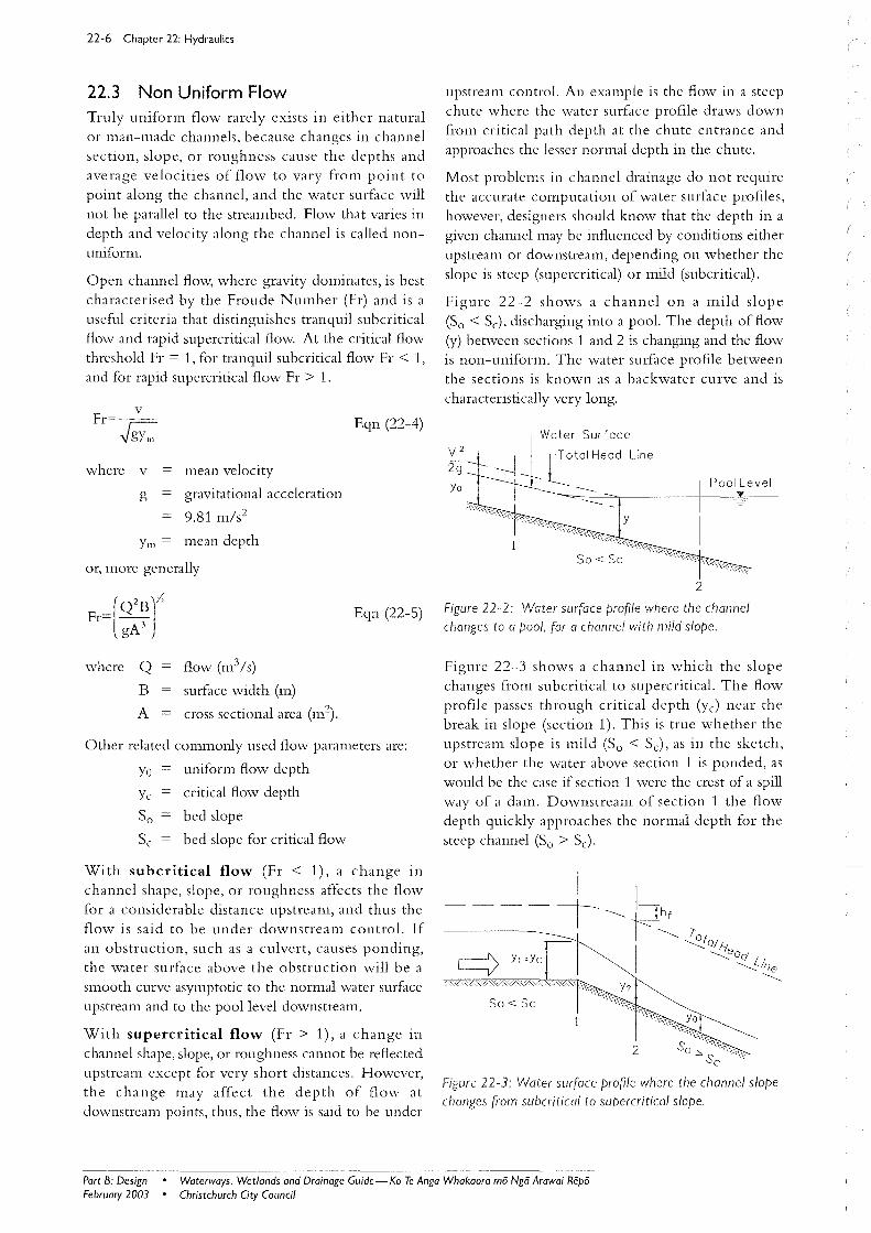
Figure 22-2 shows a channel on a mild slope (So < SJ, discharging into a pool. The depth of flow (y) between sections 1 and 2 is changing and the flow is non-uniform. The water surface profile between the sections is known as a backwater curve and is characteristically very long.

Water Surface

etal Head Line

-------Pool Level

2

Figure 22-2: Water surface profile where the channel changes to a pool, for a channel with mild slope.

Figure 22-3 shows a channel in which the slope changes from subcritical to supercritical. The flow profile passes through critical depth (y c) near the break in slope (section 1). This is true whether the upstream slope is mild (So < Sc), as in the sketch, or whether the water above section 1 is ponded, as would be the case if section 1 were the crest of a spill way of a dam. Downstream of section 1 the flow depth quickly approaches the normal depth for the steep channel (So> Sc).

Figure 22-3: Water surface profile where the channel slope changes from subcritical to supercritical slope.


• Waterways. Wetlands and Drainage Guide-Ko Te Anga Whakaora mii Nga Arawai Repii • Christchurch City Council

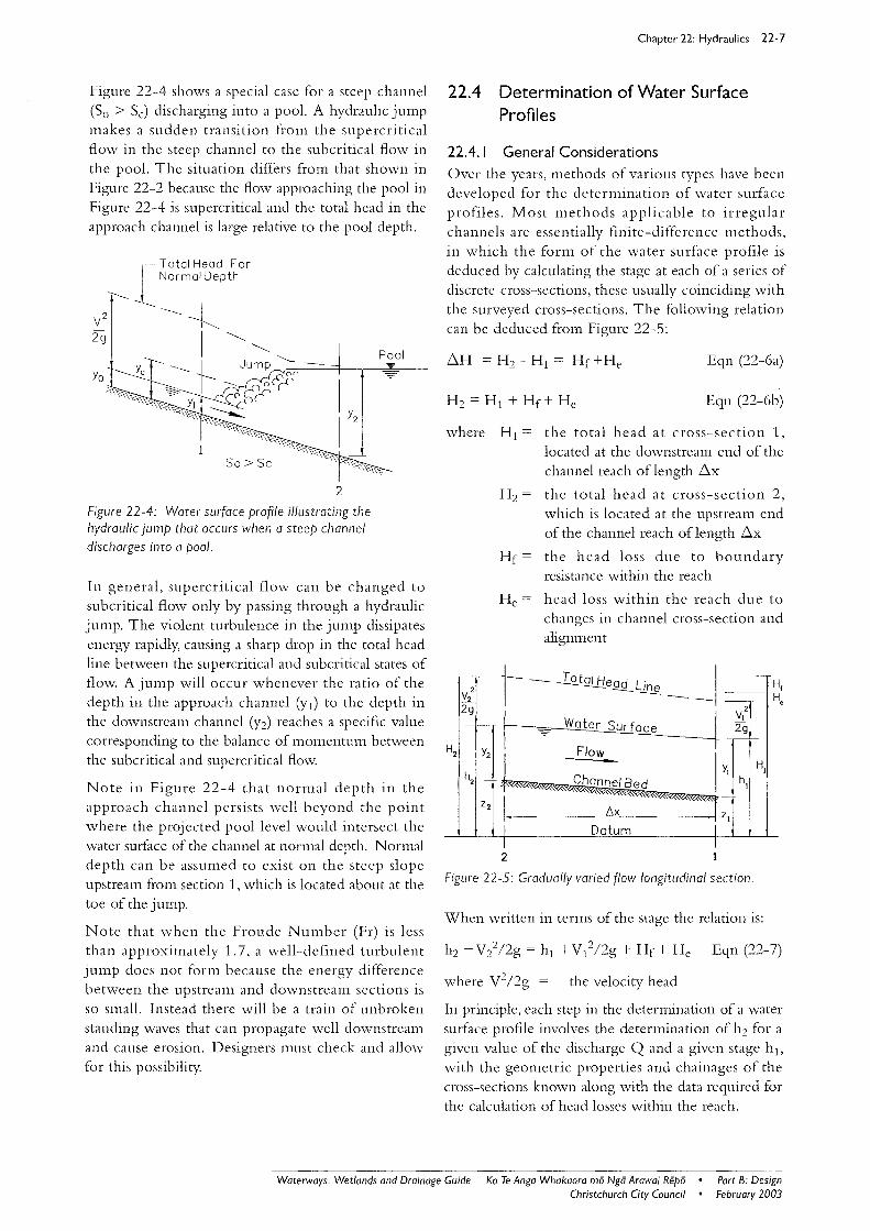
Figure 22-4 shows a special case for a steep channel (So> Sc) discharging into a pool. A hydraulic jump makes a sudden transition from the supercritical flow in the steep channel to the subcritical flow in the pool. The situation differs from that shown in Figure 22-2 because the flow approaching the pool in Figure 22-4 is supercritical and the total head in the approach channel is large relative to the pool depth.

Yo

2

Figure 22-4: Water surface profile illustrating the hydraulic jump that occurs when a steep channel discharges into a pool.

In general, supercritical flow can be changed to subcritical flow only by passing through a hydraulic jump. The violent turbulence in the jump dissipates energy rapidly, causing a sharp drop in the total head line between the supercritical and subcritical states of flow. A jump will occur whenever the ratio of the depth in the approach channel (YI) to the depth in the downstream channel (Y2) reaches a specific value corresponding to the balance of momentum bet\veen the subcritical and supercritical flow.

Note in Figure 22-4 that normal depth in the approach channel persists well beyond the point where the projected pool level would intersect the water surface of the channel at normal depth. Normal depth can be assumed to exist on the steep slope upstream from section 1, which is located about at the toe of the jump.

Note that when the Froude Number (Fr) is less than approximately 1.7, a well-defined turbulent jump does not form because the energy difference between the upstream and downstream sections is so small. Instead there will be a train of unbroken standing waves that can propagate well downstream and cause erosion. Designers must check and allow for this possibility.


22.4 Determination of Water Surface Profiles

22.4.1 General Considerations Over the years, methods of various types have been developed for the determination of water surface profiles. Most methods applicable to irregular channels are essentially finite-difference methods, in which the form of the water surface profile is deduced by calculating the stage at each of a series of discrete cross-sections, these usually coinciding with the surveyed cross-sections. The following relation can be deduced from Figure 22-5:

Eqn (22-6a)

Eqn (22-6b)

where HI = the total head at cross-section 1, located at the downstream end of the channel reach of length .6.x

v} 29 - -

H2 Y2

h2 -

Z2

H2 = the total head at cross-section 2, which is located at the upstream end of the channel reach of length .6.x

Hr = the head loss due to boundary resistance within the reach

He = head loss within the reach due to changes in channel cross-section and alignment

J --- -IQtalHead L' H ---.;. - J!J&. --- H

t 4 ~ Water Surface - --,-

1 Flow

I Y1 - HI

Channel Bed hi

I /:::'x "j-

ZI

I Datum I I I 2

Figure 22-5: Gradually varied flow longitudinal section.

When written in terms of the stage the relation is:

h2 + Vil2g = hi + Vl2/2g + Hf + He

where V2/2g = the velocity head

Eqn (22-7)

In principle, each step in the determination of a water smface profile involves the determination of h2 for a given value of the discharge Q and a given stage hi, with the geometric properties and chainages of the cross-sections known along with the data required for the calculation of head losses within the reach.

Waterways. Wetlands and Drainage Guide-Ko Te Anga Whakaora mo Ngi5 Arawai Repo • Part B: Design February 2003 Christchurch City Council •


22.4.2 Data for Determination of Water Surface Profiles

In general, the determination of a water surface profile for gradually varied flow at a given discharge is dependent upon the availability of sufficient data to define the geometry of the channel and the boundary roughness.

Definition of the channel geometry will require surveyed cross-sections extending across the full width of the channel and overbank flow areas. Close spaced cross-sec tions will be required at locations where changes in discharge, channel slope, or boundary roughness occur. In an irregular channel, the spacing and location of the surveyed cross-sections must be such that variations in the shape and size of the channel cross-section are adequately defined.

Changes in channel geometry between cross-sections sho uld be smooth and monotonic, so that, for example, the effect of a narrowing and the subsequent expansion of the channe l will be adequately represented . Cross-sections will also be required at structures such as bridges, culverts and weirs, at possible controls, and adjacent to cha nnel branches and junctions. The cross-sections should be oriented at right angles to the expected local flow direction.

22.4.3 Head Loss Due to Changes in Channel Cross-section

The term He in Eqn (22-7) represents the total head loss within the channel reach due to changes in the size and shape of the channel cross- sec tion and to changes in channel alignment.

In subcritical flow, the head loss (He) associated with a change in channel cross-section can be expressed in terms of a loss coefficient (CL) and the change in the velocity head. The expression is of the form:

H = C 6.(V2j ) c' L /2g

Eqn (22-8)

22.4.4 Head Loss Due to Change in Channel Alignment

The head loss in a channel bend can be estimated from the expression:

H - C (V2 j ) < - L /2g

Eqn (22-9)

where V the mean flow velocity in the channel at the bend

Values of the loss coefficient C L for channel bends have been discussed by Henderson (1966), who has suggested that for channel bends with deflection angles between 90 0 and 180 0

, an estimate of the loss coefficient can be obtained from the expression:

CL = 2B/r Eqn (22-10)

where B the channel width

r the radius of curvature of the channel centre-line

Henderson (1996) notes that in some cases, use of Eqn (22-10) may cause the loss coefficient to be overestimated, by factors up to about three. Where records of field observations are available it may be possible to derive values of the loss coefficients for particular sites on the basis of these records.

22.4.5 Computer Software Systems for the Determination of Water Surface Profiles

The determination of water su rface profiles in gradually varied flow can be efficiently computerised, as it involves (in the case of a channel of irregular cross-section) relatively large bodies of data and repetitive calculations. Software suitable for water profile determination includes:

HEC-RAS:

Mouse:

Mikell:

US Army Corp of Engineers

Danish Hydraulic Institute

Danish Hydraulic Institute.

the absolute difference between Tab le 22-2: Loss coefficients for a change in channel area.

the velocity heads up stream and downstream from the change in cross-section

The values given in Table 22-2, for the loss coefficient C L in Eqn (22-8), are suggested in the US Army Corps of Engineers (2001). Note that the h ead losses associa ted with channel contractions tend to be somewhat less than those associated with expansions .

I

Change Type Gradual Abrupt

Contraction 0.1 0.6

Expansion 0.3 0.8


• Waterways . Wetlands and Drainage Guide - Ko Te Anga Whakaora rnii Ngii Arawai Repii • Christchurch City Council

22.5 Outfall Water Levels Pipes and open chann els should be d es ig ned by chec kin g backwater profiles ca lculated from an appropriate o utfall water level. Failure to do so will likely result in unnecessa rily large co nduit sizes for free outlet conditions and undersized conduits for

drowned outlet conditions. At intermediate inlets and at the upp er end of a system , water levels computed from the design flow shall be low enough to prevent overflow and to allow existing and future connections to function sa tisfactorily. Systems sho uld be reviewed in the light of secondary flow characteristics Refer

to Chapter 14.6: Pipe Inlet Strtlctllres, and Chapter 14.7: Pipe Ollifall Strllctllres for further information .

If work is being designed upstream of an existing sys tem that has been designed for a lower flow, the new work should be sized as if th e old work was about to be upgrade d with a syste m ca pabl e of handling the current design flows. Similarly, the new work should be sized on the assumption that future upstrea m renewal w ill allow the passage of current design flows.

Inc rease d flow rates from new works m ay have nega tive consequ ences on lower capacity sec tions in the sho rt-term. Some consideration sho uld be given to temporary 'chokes' .

Stormwater pip elin es are often lo ca te d so as to operate in a surcharged condition at full design flow. The relationship betwee n pipe flow and head loss is shown on the pipe flow nomograph (Appelldix 11: Pipe Flow NOIl/O,~mph).

22.5.1 Tidal Outfalls

For areas with tida l o utfalls the design mu st sa tisfy th e ba si c c riteria in Table 22-3 . Alternatively it is accep table to demonstrate by full probab ility assessm ent, in combination with tidal cycle data, that the inundation performance standards of C/wpter 20: IlIlIlIdatioll D es igll Peljor/llallce Stalldards, have been sa tisfied. In additi o n , for stru ctures, allowance shall be made for sea level rise over the life expectancy of the stru cture. Adopted sea level rise valu es shall be as se t out in Appelldix 1: Defillitiolls alld Usifll/ N II/Ilbers.

When existin g development is too low to meet these criteria, each case will need to be determined according to its particular circumstances.


Table 22-3: Tidal outfall des ign water levels

Outfall Water Level Flow Scenario

Estuary Sea/Tidal River

Design storm flow

Half of design

storm flow

Typical base flow

10.30 m

10.70 m

10.85 m

10.3 m *

10.8 m *

10.9 m *

* Corresponding levels in rivers to be se t by the Christchurch

City Council.

22 .5.2 Outfalls to Rivers and Larger Waterways

When a waterway fl ows into a much larger waterway, the peak flows are unlikely to coincide. Backwater

profiles should produce sa tisfactory water levels w hen assessed for the two following scenarios.

Firstly:

a) se t tribu tary AEP based on the requirements of Chapter 20: IlIlIlIdation Desigll Pef{cmlla/l ce Standards

b) determine the tributary critical storm duration D

c) for duration D and AEP, determine the tributary

flow (Qtrib).

Determine Profile I:

This assumes that a le sse r flood is present in the receiving watelway at the time of the tributary pea k

flow arrival.

d) determine the receivin g waterway flood water level for the AEP shown in Table 22-4

e) starting with th e level from (d), determine the

tributary water profile (Profile 1) at flow Qtrib.

Table 22 -4: Recipient catchment design AEP

Tributary Catchment Area (h3)

Up to 500

500 to 800

800 to 1500

1500 plus

Recipient Catchment Area including ~ributary (ha)

Up to 500 to 800 to 1500 500 800 1500 plus

5 5 5 10

10 10 20

20 20

50

Waterways, Wetlands and Drainage Guide - Ko Te Anga Whakaora mii Ngii Arawai Repii • Part B: Design February 2003 Christchurch City Council •


Determine Profile 2:

This assumes that the tributary waterway peak flow has already passed by at the time of arrival of the receiving waterway's peak flow.

£) determine the receiving waterway peak water level at the AEP from (a) above

g) starting with level (f), determine the tributary

water profile (Profile 2) at a flow of 75 % of Qtrib

h) the design profile is the higher of Profile 1 or 2.

22.6 Afflux at Bridges and Other Structures

22.6.1 Introduction

The design guide here is ancillary to Chapfer 13.2: Bridges alld CII/perfs, which should be read first.

The provision of a bridge or other structure within a channel often involves a constriction of the channel since, with the objective of reducing the cost of the structure, the width of the waterway at the structure is commonly made less than the width of the channel upstream and downstrealTl. As a result, the flow accelerates as it approaches the structure and passes through the constructed waterway at the structure with a velocity greater than that of the approach flow. A subsequent deceleration of the flow occurs downstream from the structure, as the flow expands into the unconstricted channel downstream.

If no loss of head occurred, then water levels in the channel would be affected only in the immediate vicinity of the structure. This is provided that the channel width at the constriction is greater than the limiting value that would cause the occurrence of critical flow at the constriction. In reality however, head losses will occur as a result of the acceleration and deceleration of the flow.

The total head loss through the structure will be the sum of these head losses, together with the head loss due to boundary resistance. In most cases a large proportion of the total head loss will occur in the expansion of the flow downstream from the structure. If the flow in the channel is su bcritical, the head loss through the structure will cause an increase in water levels upstream from the structure; this increase in water levels is commonly referred to as "affiux" or "backwater".

Procedures for assessing afflux are described in Pilgrim (1987).

22.6.2 Effect of Channel Scour on Afflux

Increased velocities that will occur in the constructed waterway at a bridge will tend to scour material from the channel bed in the vicinity of the structure.

Where scour of the channel bed is expected, it is necessary to examine the effect of this scour on the stability of bridge piers and abutments and on any other natural or artificial feature likely to be affected.

22.7 Bed Shear Stress and the Stable Bed Stability of a substrate depends on the gravitational restraining force exceeding the fluid drag force. The average fluid drag on the water/substrate interface can be expressed as a bed shear stress, also known as "tractive force", as below:

TO = '1RS (N/ni) Eqn (22-11)

where '1 pg (N/m3)

p 1000 kg/m3

fluid density

g 9.81 m/s2

R hydraulic radius (m)

S friction slope (m/ m)

approx water surface slope

Low Turbulence Flow

If flow turbulence is low (typically y / d75 > 5 and Fr <1.5 where y = water depth) then the US Bureau of Reclamation recommended safe value of shear

stress To for noncohesive materials greater than 6mm diameter can be determined frOlTl Eqn (22-10; refer, Henderson 1966, Pg417). d75 is the reference particle size because it is this size that tends to armour the natural stream.

Eqn (22-12)

Where d75 is in mm

Combining Eqn (22-11) and Eqn (22-12) an expression is obtained that enables the stable d75 size to be obtained directly for a wide channel:

d75 = 11RS

where d75 IS 111 m

R IS 111 m

S is in m/ I1l

Eqn (22-13a)

For a channel of shallow parabolic cross section the

peak bed shear stress on the line of maximum depth is higher than the average value of (22-13a), thus:


• Waterways. Wetlands and Drainage GUide-Ko Te Anga Whakaora rna Nga Arawai Repa • Christchurch City Council

Chapter 22: Hydraulics 22-1 1

d7s = 19R5 Egn (22-13b) High Turbulence Flow

Eguation (22-13b) above, can be combined wi th the following Strickler formula for M anning's n:

n = 0.012d1!6 Eqn (22-14)

where d d7s (mm)

and Manning's Eqn (22- 1) to give a sa fe maximum channel slope, thus:

If flow turbulence is high (typically y/dso < 5 and Fr > 1. 5) then use Eqn (22-16) based on the Isbash formula. Note that Isbash (1936) based his work on placed material based on dso size rather than d7s used for Low Turbulence Flow design above.

Eqn (22-1 6)

S = 33d l1 SQ -0.46 (ml m)

where d I S 111 m

Q is in m3/s

Egn (22-15) Here K incorpora tes an allowance for the degree of turbulence and stone angle of internal friction. For strong turbulence above a well-interlocked bed of very angular material of basalt or greywacke (specific

Table 22-5 below includes a tabulation of velocity limit values at y/ d7s = 5. For y/d7s > 5 the se velocities will be conservative and so the designer could instead make use of Eqn (22-1 5) to directly assess bed stability.

Table 22-5: Stable bed velocities

Isbash Eqn(22-13) yld = 5

dso (m) vel (m/s) d7s (m) V nux (m/s)

0.003 0.40

0.006 0.60

0.010 0.75

0.020 1.0 0.020 1.1

0.030 1.2 0.030 1.3

0.040 1.4 0.040 1.6

0.060 1.7 0 .060 1.9

0.080 1.9 0.080 2.2

0.100 2.2 0.100 2.5

0.120 2.4 0.120 2. 7

0.150 2.6 0.150 3.0

0 .200 3.1 0.200 3.3

0.250 3.4

0.300 3.7

0 .350 4.0

0.400 4.3

0.450 4.6

0.500 4.8

0.600 5.3

0.700 5.7

0.800 6. 1

0.900 6.5

1.000 6.8

gravity > 2.4), and shape factor no greater than 3, K may be taken as 0.42. This value is consistent with recommendations of the MWD C ulvert Manual (Ministry of Works and D evelopment 1978) . Shape factor is defined as rock maximum dimension divided by minimum dimension.

Where downstream bed slope is > 5 % then multiply dso by:

n1a = sin(<I»

sin(<I>-~)

where <I> angle of repose

45° for broken rock

30° for round rock

~ slope angle

For channel side slope, multiply dso by:

1 mh = ----;=====

1- ( sin ~ ) S111 <I>

Eqn (22-17)

Egn (22-18)

Achievement of a "well interlocked" bed is likely to require a layer thickness of at leas t 2dso on top o f smalle r sized sco ur res ista nt underlayers. The larges t rocks (d 100) should fit within this layer and no more than 15 % of rock should be smaller than 0.6dso. Rock should be so und, durable stone, free from cracks and seams. Deleterious material including soft, friable particles should not exceed 5 %.

For granular bed materials, and Fr > 1.5, flow j etting must not be able to penetrate the voids beneath the armouring beca use of the uplift pressures that m ay develop. In such situations the filling of voids w ith cohesive material is recommended. Stron gly rooted grass cover or tree root matting can assist in reducing velocities and increasing scour resistance.

Waterways, Wetlands and Drainage Guide-Ko Te Anga Whakaora ma Nga Arawai Repa • Christchurch City Council •

Part B: DeSign February 2003


Silt or Sand Substrate

For sand or silt stream beds the assessment is less straightfonvard; there is nearly always some sediment movement, the suspended sediment load affects bed shear stress, and for fine substrates, the channel roughness relates to factors other than particle size. Work by Simons and Albertson (as outlined by Henderson 1966), could be considered. In the absence of other information, assume a V max of 0.3 m/s for silt or sand substrates.

22.8 Riffle, Run, Pool DeSign Portions of a river are often characterised as riffle, run, or pool. Riffles are shallow swift flowing areas with broken water surface and larger substrate (gravel, cobbles, or boulders). Pools are deeper slow flowing areas with an almost level smooth water surface and often containing deposits of finer substrate (sand or gravel). Runs are intermediate between pools and riffles and are characterised by an undulating but relatively unbroken water surface.

These classifications appear to best relate to the Froude Number (Fr) that relates inertial forces to gravity forces. This is important hydraulically wherever gravity dominates (e.g. waves and open channel flow), and is the criteria that distinguishes tranquil and rapid flow such as occurs in riffles, runs and pools. See also Chapter 22.3: NOll Ulli{orlll FlO/I!.

The basic Froude NU111ber equation repeated here is:

Fr= __ v_ c::- Eqn (22-4) "gym

where v mean velocity

g gravitational acceleration

9.81 m/s2

Ym = nLean depth

The riffle, run, pool criteria are further described in Chapter 9.3.2.1 : Des(~11 COllsidemtiolls Jor Riffles, and shown graphically on Figure 9-5.

The riffle/run threshold is set to: Fr = 0.35

The run/pool threshold is set to: Fr = 0.15

Riffle, Run, Pool Design Steps

1) assume a riffle height and slope; say 100 111m height, 1: 100 grade, 10 m length

2) space the riffles as per Chapter 9.3.2: Riffle, RIIIl, Pool Seqllcllces

3) assume an intermediate run gradient of say 1 :500

4) analyse the channel for "normal" base flow as might occur in say, December

5) ensure the riffle criteria of Figure 9-5 are met (see Chapter 9.3.2.1: Dcs~,<" COllsideratiolls Jor Riffle:,)

6) adjust the riffle/run gradients and riffle spacings as required, then repeat step 4

7) re-analyse the channel for a 6 month "flood" flow

8) determine the minimum d75 size using either Eqn (22-13b) or Table 22-5

9) repeat for larger flood events to ensure the d75

remains stable

10) ensure the bed shear stress is sufficient to sweep clear any surface sand size particles or smaller.

The final substrate should have a d75 size at least as large as determined above, but can be larger. d75

should ideally be in the range of 16-160 mm. There should be a good mixture of particle sizes.

22.9 Hydraulic Design of Culverts and Pipes

The design guide here is ancillary to Chapter 13.2: BridJ!.es alld CIIIFcrts, which should be read first.

The content of this section is adapted from the Australasian Concrete Pipe Association's hydraulic design manual (Concrete Pipe Association of Australasia 1994), which should be referred to for additional guidelines and design charts.

Culverts, despite their apparent simplicity, are complex engineering structures from a hydraulic as well as a structural viewpoint. Their function adequacy is no better than the estimate of the design flood, and the hydraulic design described below must be preceded by a careful flood evaluation together with an assessment of effects caused by the design flood being exceeded or blockage of the culvert entry.

The hydraulic complexity of culverts is a result of the many parameters influencing the flow pattern. This influence can be summarised to two major types of culvert flow control:

flow with inlet control

flow with outlet control

both of which require evaluation to determine which will govern.

While the hydraulic design of culverts and pipes is critical, design must also consider ecological and aesthetic values. Refer to Chaptcr 13.2.3: DesiJ!.llillR Fish Friclldly CIIIFcrts alld vVcirs, and other sections in Chapter 13.2: BridJ!.es alld CIIlperts, for more information.


• Waterways. Wetlands and Drainage GUide-Ko Te Anga Whakaora mo Ngo Arawai Repo • Christchurch City Council

22.9. I Types of Culvert Flow Control

Determination of Operating Condition

The most restrictive of the two flow types, inlet control or outlet control , applies, that is, the one giving least discharge for given headwa ter level, or requiring higher headwater level for given discharge.

Flow with Inlet Control

Culvert flow is restricted to the discharge tha t can pass the inlet with a given headwater level (see Figure 22- 6):

The discharge is co ntroll ed by the headwater depth, the cross-section area at the inlet, and the geometry of the inlet edge. It is not appreciably affected by length, roughn ess, slope , or outlet conditions, and the culvert is not flowing full at any point except perhaps at the inlet. This culvert type is mostly short or steep.

The culvert flow is restricted to the discharge which ca n pass through the pipe and ge t away from the outlet with a given tailwater level (Figure 22-6):

The culvert can run full over at least some of its length. The discharge is affected by the length, slope, roughness, and outlet conditions, in addition to the depth of headwater, the cross-sec tion area, and inlet geometry.

UNSUBMERGED

HW

t ~-- - -- --Figure 22-6: Inlet flo w control.

Flow with Outlet Control

The simplest case of outlet control is illustrated in Figures 22-7 a and 22-7b. Here the culvert is flowing full for its en tire length . The energy head (b.H) required to maintain this flow equates to the su m of the losses and can be expressed.

where Hv

He

velocity head

V2/2g

entry loss

keHv

friction loss

Eqn (22-19)


The en trance loss coefficient ke is given in Table 22-6 for various pipe and box culvert entry conditions and culverts flowing with ou tlet control.

Table 22-6: Entrance loss coefficient (ke).

Culvert Entrance Type ke

Pipe Culverts

Pipe projecting from fill:

square cut end

socket end

Headwall with or without wingv,Ialls:

square end

socket end

Pipe mitred to conform to fill slope:

precast end

field cut end

Box Culverts

0.5

0.2

0.5

0.2

0.5

0.7

No wing walls, headwall parallel to embankment:

square edge on 3 edges 0.5

3 edges rounded 1/12 barrel dimension 0.2

Wing walls at 30 to 75 to barrel:

square edge at crown 0.4

crown rounded to 1/12 culvert height 0.2

Wing wall at 10 to 30 to barrel:

square edge at crown

Wing walls parallel (extension of sides):

square edge at crown

HW[ ~/ ./

I laJ

leJ

IdJ

Figure 22 -7: Outlet flow control.

....,

~ "-......,

..

0.5

0.7

l:j::

Waterways . Wetlands and Drainage Guide-Ko Te Anga Whakaora rna Nga Arawai Repa • Christchurch City Council •


22-14 Chapter 22: Hydrau lics

Note: the velocity head term above (Hv) is required at the entrance to accelerate the flow to velocity V It is then lost at the exit due to sudden expansion.

The friction loss (Hr) is ideally calcula ted from the Colebrook-White eq uation but is more readily and more widely calc ulated using the Manning formula . See Serfioll 22.2.2: The lVlal'l llillg ForlllII la.

For circular culverts flowing full, Manning's formula reduces to:

Eqn (22-20)

From which the friction loss (HO can be determined as:

H r = L.Sr Eqn (22-21)

Knowing the energy differential head (.0.H) and tailwater level (TW), the headwater (HW) can be calculated fr011'1 the equation:

HW =TW +.0.H - L.So

where L

So

culvert length

culvert slope

Eqn (22-22)

For culverts and pipes not flowin g full, refer to Concrete Pipe Association of Australasia (1994).

22.9.2 Headwater

Headwater (HW) is the depth of water at the inlet above the invert of the culvert . It is influenced by factors such as:

acceptable upstream flooding

culvert flow velocity

overtopping of the roadway

the possibility of water penetration into the embankment.

Culvert hydraulic performance criteria are set out in Chapfer 13.2: Bridges alld C lll ile rfs, and Chapfer

14: Pipelille Sfrllcfllres.

22.9.3 Tailwater

Tailwater (TW) is the depth from the natural wate r surface at the outlet to the invert of the culvert. The tailwater level may be governed by downstream obstructions or the discharge from other streams.

22.9.4 Freeboard

Freeboard is the distance between the headwater level and the crown of the culvert. See Chapfer 13.2.2: Des(en CO llsidemfiolls.

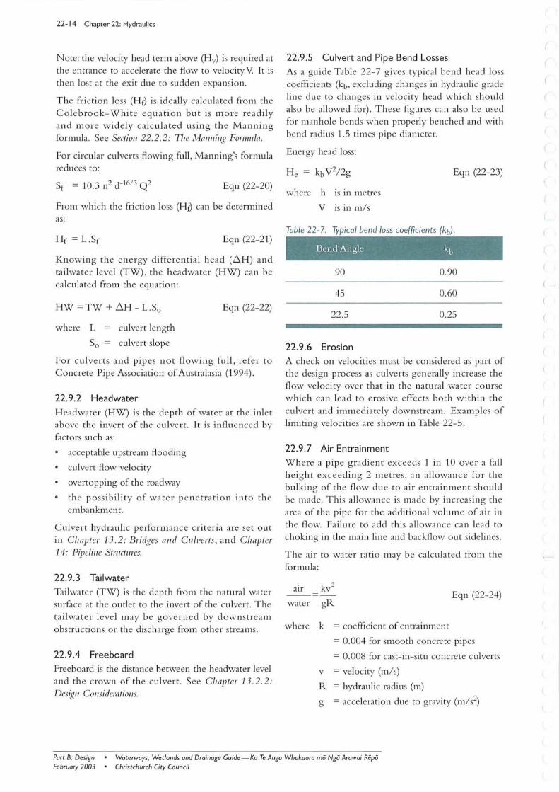
22.9.5 Culvert and Pipe Bend Losses

As a guide Table 22-7 gives typical bend head loss coefficients (kb, excluding changes in hydraulic grade line due to changes in velocity head which should also be allowed for) . These figures can also be used for manhole bends when properly benched and with bend radius 1.5 times pipe diameter.

Energy head loss:

where h is in metres

V is in m l s

Eqn (22-23)

Table 22-7: Typical bend loss coefficients (kbJ .

Bend Angle kb

90 0.90

45 0.60

22.5 0.25

22.9.6 Erosion

A check on velocities must be considered as part of the design process as culverts generally increase the flow velocity over that in the natural water course which can lead to erosive effects both within the culvert and immedia tely downstream. Examples of limiting velocities are shown in Table 22-5.

22.9.7 Air Entrainment

Where a pipe gradient exceeds 1 in 10 over a fa ll height exceeding 2 m etres, an allowance for the bulking of the flow due to air entrainment should be made. This allowance is made by increasing the area of the pipe for the additional volume of air in the flow. Failure to add this allowance can lead to choking in the main line and backflow out sidelines.

The air to wa terra tio may be calcu la ted from the formula:

water gR Eqn (22-24)

where k = coefficient of entrainment

= 0.004 for smooth concrete pipes

= 0.008 for cast-in-situ concrete culverts

v = velocity (m / s)

R = hydraulic radius (m)

g = acceleration due to gravity (m/s2)


• Waterways, Wetlands and Drainage Guide-Ko Te Anga Whakaora mii Ngo Arawai Repii • Christchurch City Council

( J

Having determined the pipe size for 'basic' water flow, pipe size should be increased to provide cross-section area for 'water + air'. This equates to scaling the basic diameter for water alone as in Eqn (22-25).

dia = 1+~ [

k 2j)l, reqd. gR dia !>.\Sic Eqn (22-25)

22.9.8 Siltation

If the flow velocity becomes too low, siltation will occur. Flow velocities below about 0.5 m /s will cause se ttlement of fine to medium sand particles.

Siltation in pipes and culverts mostly occurs if they are placed at incorrec t levels leading to low velocity in the pipe or culvert that is lower than the average stream flow.

To be self-cleaning culverts must be graded to the ave rage grade of the watercourse upstream and downstream of the culvert , and water levels must represent the average stream levels before the culvert was built.


22. 10 Sumps - Collection of Water from Side Channels

22.10.1 Side Channel Flow Capacity

Standard side channels are shown on standard details SD601 and SD604 included in the Construction Standard Specification , CSS: Parts 2 and 3 (see Christchurch City Council 2002a, b). Flow capacities are shown in Table 22-8.

In no case shall a side channel be designed to convey more than 175 lis. The designer should note that where velocity exceeds 1.5 m/s there is a danger of erosive damage to the pavement and special topcourse and pavement design may be required to guard against this. Alternatively the flow should be entirely contained within the fender.

Care should be exercised with flow around bends when velocity is greater than 1m/s as momentum will tend to lift flow out of the channel. Channel reduced capacity around bends can be derived by assuming a water slllface crossfall from Eqn (22-26). Plotting this

Tab le 22-8: Side channel flow capacity (based on Manning's n = 0.0/6) .

500 0 .0020 50 0.40 130 18 0.45 165

400 0.0025 55 0.44 130 20 0.51 165

300 0 .0033 64 0.51 130 23 0.59 165

200 0.005 78 0.62 130 29 0.72 165

100 0.010 110 0.88 130 41 1.0 165

70 0 .014 130 1.1 130 49 1.2 165

50 0.020 155 1.2 130 57 1.5 165

40 0.025 175 1.4 130 5 0.68 40 64 1.6 165

30 0.033 175 1.6 125 6 0.79 40 75 1.9 165

20 0.050 175 1.8 117 7 0.96 40 75 2.2 155

15 0.067 175 2.0 112 9 1.11 40 75 2.5 145

10 0.100 175 2.4 105 10 1.36 40 75 2.9 130

8 0.125 175 2.6 100 12 1.52 40 75 3.1 125

6 0.167 175 2.9 95 13 1.76 40 75 3.5 115

4 0.250 175 3.4 90 17 2.15 40 75 4.1 105

Unshaded flows are depth limited. Shaded fl ows are set capacity limits. Capacity must be reduced around bends (see Chapter 22. 10. 1: Side Challllel FlolIJ Capacity) .

Waterways . Wetlands and Drainage Guide-Ko Te Anga Whakaora rnii Ngo Arawai Repii • Part B: Design Christchurch City Council • February 2003


crossfall on the appropriate standard detail will give a flow area reduction that can be taken as proportional to the flow obtained from Table 22-8.

crossfall = v2/gr towards inside of bend Eqn (22-26)

where v = velocity from Table 22-8

r = bend radius to centreline of flow

g = 9.81

e.g. v2 I gr 0.2

1 in 5 water surface crossfall

22.10.2 Sump Capacity

The standard flat channel and hillside channel grate types referred to here (SD324 and SD325), are shown in the CCC Construction Standard Specification CSS:Part3 (Christchurch City Council 2002b). Capacities of sump gratings shown below allow for partial blockage of the sump.

Note: The capacities shown here allow for partial blockage of the sump grating.

Standard Flat Channel Sump (S0325)

Inline sump capacity 20 lis per grating unit

Valley position capacity = 40 lis per grating unit

Note that this type of sump grating has a much reduced capacity if the flow velocity exceeds 1 m/s.

Standard Hillside Sump (S0324)

The maximum capacity of the standard hillside sump shall be taken as 80 lis for the 2 m length shown on SD324 but this detail can be altered in length as required based on 40 lis per m length provided a check is made on the flow capacity of the outlet, especially the pipe entrance. The channel beneath the grate may also require enlargement for grating lengths greater than 2 m.

This type of grating may have difficulty with flow interception if velocity exceeds 2.5 m/s.

22. I I Weirs and Free Overfalls

22. 1 1 . 1 Weirs

Formulae are presented here for three common weir types. Formulae for other weir profiles can be found in many hydraulic textbooks.

Sharp Crested Weirs

The formula for flow over a sharp crested weir of infinite width and infinite upstream depth is:

Eqn (22-27)

Where approach depth is shallow, replace the discharge coefficient 1.8 with (1.8 + 0.23 H/W) where H is upstream water level height above the weir crest (metres) and W is weir crest height above upstream invert (metres).

For rectangular weirs, side contraction can also be significant. To allow for side contraction replace crest width B with (B - 0.2 H).

Broad Crested Weirs

Eqn (22-28) is applicable where the crest length in the flow direction is approximately 3H and the weir has a rounded leading edge. For greater crest length, boundary layer effects reduce the discharge coefficient.

Q = B X 1. 7 H l.5 Eqn (22-28)

Ogee Weir

This is the classic parabolic like weir profile for which:

Q = B X 2.2 H l.5 Eqn (22-29)

22.11.2 Free Overfalls

The gravity free trajectory parabola, beginning with horizontal velocity (v) and zero vertical velocity, is defined by:

Eqn (22-30)

where y = the vertical fall below the lip

x = the horizontal distance from the lip

v = the initial horizontal velocity

Residual internal pressure at a free overfall yields a depth and velocity above critical at the lip, leading to a brink depth (Yb) of 0.715yc and velocity Vb

approximately 1.5vc. This initial velocity can be applied to Eqn (22-30) to give an approximation to the centreline of the free overfall jet.

For thin, decorative water£l11s, smface tension can lead to significant lateral contraction of the free falling jet. To minimise this contraction and other effects, the flow should be at least 6 lis per metre width and depth (y c) should be greater than 15 mm.

Part B: Design • Waterways. Wetlands and Drainage Guide-Ko Te Anga Whakaora mii Ngii Arawai Repii February 2003 • Christchurch City Council


22. 12 References Barnes, H. H. Jr. 1967. Roughness Characteristics of Natural Channels. US Departlllent 4 the InteriO/; Geological SlIrlley TIVater-Sllpply Paper No 1849. Now maintained as document manningN.pdf (5MB) on the US Geological Survey web site at address: http: / /www.rcamnI.wr.usgs.gov/sws/fieldmethods/ Indirects/ nvalues/ index. htm

Brater, E. F & King, H. W. 1976. Handbook (:f Hydra II lics for the Soilltion of Hydralllic Engineering Problellls (6th ed.). McGraw-Hill, New York.

Chow,V:T. 1959. Open-Cllilllllei Hydralllics. McGrawHill, New York.

Christchurch City Council 2002a. Constl"llction Standard Specification (CSS), Part 2: Earthworks. Christchurch City Council, Christchurch. Available from: http:www.ccc.govt.nz/Doing Business/ css/

Christchurch City Council 2002b. Constl"llction Stal1dard Specification (CSS), Part 3: Utility Pipes. Christchurch City Council, Christchurch. Available from: http:www.ccc.govt.nz/Doing Business/ css/

Concrete Pipe Association of Australasia 1994. Hydraulics of Precast Concrete Conduits, Pipes and Box Culverts. Hydraulic Design Manual. Concrete Pipe Association of Australasia, Auckland.

French, R. H. 1985. Opell-Channe! Hydral/lics. McGraw-Hill, New York.

Henderson, F. M. 1966. Opell Channel Flow. MacMillan, New York.

Hicks, D .M. & Mason, P. D. 1991. Roughness Characteristics of New Zealand Rivers. Water Resources Survey, DSIR Marine and Freshwater, Wellington.

Isbash, S.V: 1936. Construction of dams by depositing rock in running water. 7iwlsaction, Second COllgress on Lm~t,ze Dallls 5: 123-126.

Ministry of Works and Development 1978. Culvert Manual- CDP 706. Civil Division, Ministry of Works and Development, Wellington.

Pilgrim, D. H. (ed.) 1987. Allstralian Rainfall and RIII/{:ff: A G/lide to Flood Estimation, Voillme 1. The Institution of Engineers, Barton.

US Army Corp of Engineers, Hydrologic Engineering Centre 2001. HEC-RAS Hydraulic Reference Manual. Davis, California.

Waterways, Wetlands and Drainage Guide-Ko Te Anga Whakaora mii Ngii Arawai Repii • Christchurch City Council •


Waterways, Wetlands and Drainage Guide - Part B: … · Waterways. Wetlands and ... scour...

Documents

Transcript of Waterways, Wetlands and Drainage Guide - Part B: … · Waterways. Wetlands and ... scour...