HAL Id: hal-01874967https://hal.archives-ouvertes.fr/hal-01874967

Submitted on 15 Sep 2018

HAL is a multi-disciplinary open accessarchive for the deposit and dissemination of sci-entific research documents, whether they are pub-lished or not. The documents may come fromteaching and research institutions in France orabroad, or from public or private research centers.

L’archive ouverte pluridisciplinaire HAL, estdestinée au dépôt et à la diffusion de documentsscientifiques de niveau recherche, publiés ou non,émanant des établissements d’enseignement et derecherche français ou étrangers, des laboratoirespublics ou privés.

Hybrid Check Node Architectures for NB-LDPCDecoders

Cédric Marchand, Emmanuel Boutillon, Hassan Harb, Laura Conde-Canencia,Ali Ghouwayel

To cite this version:Cédric Marchand, Emmanuel Boutillon, Hassan Harb, Laura Conde-Canencia, Ali Ghouwayel. HybridCheck Node Architectures for NB-LDPC Decoders. IEEE Transactions on Circuits and Systems I:Regular Papers, IEEE, 2019, 66 (2), pp.869-880. �10.1109/TCSI.2018.2866882�. �hal-01874967�

1

Hybrid Check Node Architectures for NB-LDPC

DecodersCedric Marchand, Member, IEEE, Emmanuel Boutillon, Senior Member, IEEE, Hassan Harb,

Laura Conde-Canencia, Member, IEEE, and Ali Al Ghouwayel, Member, IEEE,

Abstract—This paper proposes a unified framework to de-scribe check node architectures of Non-Binary LDPC de-coders. Forward-Backward, Syndrome-Based and Pre-sortingapproaches are first described. Then, they are hybridized in aneffective way to reduce the amount of computation required toperform a check node. This work is specially impacting checknodes of high degrees (or high coding rates). Results of 28 nmASIC post-synthesis for a check node of degree 12 (i.e. code rateof 5/6 with a degree of variable equal to 2) are provided for NB-LDPC over GF(64) and GF(256). While simulations show almostno performance loss, the new proposed Hybrid implementationcheck node increases the hardware and the power efficiency bya factor of six compared to the classical Forward-Backwardarchitecture. This leads to the first ever reported implementationof a degree 12 check node over GF(256) and these preliminaryresults open the road to high decoding throughput, high rate,and high order Galois Field NB-LDPC decoder with reasonablehardware complexity.

Index Terms—NB-LDPC, Check Node, syndrome-based, VLSI,Foward-Backward.

I. INTRODUCTION

LOW-Density Parity-Check (LDPC) codes [1] have now

been adopted for a wide range of standards (WiMAX,

WiFi, DVB-C, DVB-S2X, DVB-T2) because of their near-

channel-capacity performance. However, the capacity achiev-

ing performance is obtained for long codeword lengths and

LDPC codes start to show their weakness when considering

short and moderate codeword lengths. In the last decade

significant research effort has been devoted to the extension

of LDPC codes to high-order Galois GF(q) (q > 2 is the

order of the GF). This family of codes, named Non-Binary

(NB) LDPC codes, show strong potential for error correction

capability with moderate and short codeword lengths [2]. This

is mainly due to the fact that NB-LDPC codes present higher

girths than their binary counterparts, and thus present better

decoding performance with message passing algorithms. Also,

the NB nature of such NB-LDPC codes makes them suitable

for high-spectral-efficiency modulation schemes where the

constellation symbols are directly mapped to GF(q) symbols

[3]. This mapping bypasses the marginalization process of

binary LDPC codes that causes information loss. NB-LDPC

codes becomes serious competitors of classical binary LDPC

and Turbo Codes in future wireless communication and digital

video broadcasting standards.

The main drawback of NB-LDPC codes is related to their

high decoding complexity. In the NB-LDPC decoder each

message exchanged between the processing nodes is an array

of values, each one corresponding to a GF element. From an

implementation point of view, this leads to a highly increased

complexity compared to binary LDPC decoding.

A straightforward implementation of the Belief-Propagation

(BP) algorithm for NB-LDPC results in a computational

complexity of the order of O(q2) [2]. The Extended Min-

Sum (EMS) algorithm, which is an extension of the well-

known Min-Sum algorithm from the binary to the NB do-

main, represents an interesting compromise between hardware

complexity and error correction performance [4] [5]. As the

Check Node (CN) processing constitutes the computational

bottleneck in the EMS decoding, much research work has

focused on its complexity reduction. Currently, state-of-the-

art architectures apply the Forward-Backward (FB) algorithm

[5] to process the CN. With this approach, a serial calculation

is carried out to reduce the hardware cost and to reuse results

from intermediate Elementary CN (ECN). However, the FB

CN structure suffers from high latency and low throughput.

The Trellis-EMS (T-EMS) introduced in [6] avoids the long

latency of the FB computation but its hardware complexity

highly increases with q when a parallel implementation is

considered. The complexity of the T-EMS was reduced with

the one-minimum T-EMS [7] and the Trellis Min-Max (T-MM)

[8] [9] algorithms.

The SB algorithm, recently presented in [10] [11], is an

efficient method to perform a parallel computation of the

CN when q ≥ 16. This architecture was used for the first

reported implementation of a GF(256) CN processor with

degree dc = 4 [12]. However, the complexity of the SB CN

algorithm is dominated by the number of syndromes to be

computed, which increases quadratically with dc, limiting its

interest for high coding rates, i.e. for high dc values. Recently,

we showed that sorting the input vector of the CN according

to a reliability criteria [13] [14] allows significant reduction

of the hardware complexity of the CN architecture without

affecting performance. This technique, called “presorting”, has

been successfully combined with the SB CN, leading to the

PreSorted-SB CN (or PS-SB CN) algorithm [13] and with the

FB CN, leading to the PS-FB CN [14].

The goals of this paper are twofold. The first one is

to synthesize several contributions published in conference

papers in an unified framework. The second goal is to present

a simplification of the Extented Forward (EF) architecture

and several original hybridizations of existing architectures

to further reduce the hardware complexity of the CN and

to derive efficient hardware implementations for high-order

GF and/or high CN degrees. The pre-sorting is the key to

understand the efficiency of the Hybrid architecture compared

2

TABLE ICN ARCHITECTURES BASED ON THE EMS ALGORITHM.

CN architectures Input processing

Full form Normal PreSorted (PS)

T-EMS Trellis EMS [6] [7] -

T-MM Trellis Min-Max [8] [9] -

FB Forward-Backward [5] [15] [16] [14]*

SB Syndrome-Based [10]* [11]* [12] [13]*

EF Extended Forward-SB [17]* [17]*, this paper

HB Hybrid - This paper

to previous algorithm. Pre-sorting allows to match locally the

processing algorithm (SB, EF or FB) with the dynamic of

incoming and intermediate messages. Table I presents the

names of the different existing and proposed architectures.

In this Table, the references with an asterisk correspond to

previous contributions of the authors.

The paper is structured as follows: Section II recalls the

structure of a NB-LDPC code and presents the EMS decoding

algorithm. Section III gives a survey of the existing practical

EMS architectures. Section IV presents several original hybrid

architectures and Section V provides synthesis and perfor-

mance results. Finally, conclusions are drawn in Section VI.

II. NB-LDPC NOTATIONS AND DECODING

This section first recalls the principles and notations of NB-

LDPC codes. Then, the EMS algorithm is described.

A. NB-LDPC code

A NB-LDPC code is a linear block code defined by a

sparse parity-check matrix H of size M × N . The M rows

of the matrix H refer to M parity check equations. The ith

parity check equation is defined as dc(i) non-zero GF(q) values

{hi,ji(k)}k=1...dc(i) of the ith line of the parity check matrix

as

dc(i)∑

k=1

hi,ji(k)x(ji(k)) = 0, (1)

where {x(ji(k))}k=1...dc(i) is a subset of size dc(i) of the NGF(q) symbols of the code. A NB-LDPC code is regular if the

number dc of non-zero values per row and the number dv of

non-zero values per column are constants. Efficient NB-LDPC

coding schemes can be constructed with dv = 2 [18]. In this

case, assuming a full-rank parity-check matrix H, the rate of

the code is r = 1− 2/dc.

B. EMS algorithm

For simplicity, the EMS algorithm is described only at the

CN level. The reader can refer to [19] for a complete descrip-

tion of the whole decoding process including the variable and

edge nodes.

Fig. 1 shows a CN and its dc = 4 conected Varible Nodes

(VN). Let us define a CN equation of degree dc in GF(q) as

e1⊕ e2⊕ e3⊕ . . .⊕ edc= 0, where ⊕ represents the addition

over GF(q) 1 and ek = hi,kxk. Each input ei is a variable

1or, equivalently, subtraction in GF(q).

Fig. 1. Message notation on a CN

defined in GF(q) and its associated a priori information is the

discrete probability distribution P (ei = x), x ∈ GF(q). Each

element of the probability distribution E associated to e can

be expressed in the logarithmic domain as the Log-Likelihood

Ratio (LLR) e+(x) defined as

e+(x) = − log

(

P (e = x)

P (e = x)

)

, (2)

where x is the hard decision on e obtained with the maximum

likelihood criterion, i.e. x = argmaxx∈GF(q) P (e = x). From

this LLR definition: e+(x) = 0 and ∀x ∈ GF(q), e+(x) ≥ 0.

The distribution (or message) E associated to e is thus E ={e+(x)}x∈GF(q).

The EMS algorithm is an extention of the Min-Sum aiming

at reducing the complexity of NB-LDPC decoders. Its main

characteristic is the truncation of the messages E from q to

the nm most reliable values (nm ≪ q). At the CN level, each

incoming message U is composed of nm couples sorted in

increasing order of LLRs (note that a high LLR value means

low reliability). In Fig. 1, each input U of the CN is a list

{U [j]}j=0...nm−1 of couples U [j] = (U+[j], U⊕[j]), where

U+[j] is the (j + 1)th smallest LLR value of E and U⊕[j]is its associated GF element, i.e., e+(U⊕[j]) = U+[j]. Note

also that U+[0] = 0, U⊕[0] = x, and that j ≤ j′ ⇒ U+[j] ≤U+[j′]. The same representation is used for each output V of

the CN.

The EMS algorithm can be described in two steps:

Computation:

v+i (x) = min

dc∑

i′=1,i′ 6=i

U+i′ [ji′ ] |

dc⊕

i′=1,i′ 6=i

U⊕i′ [ji′ ] = x

,

(3)

where ji′ ∈ {0, 1, . . . nm − 1} for i′ = 1, 2, . . . dc, i′ 6= i.Sorting: the v+i (x) are sorted in increasing order and the

first nm smallest values are kept to generate the output vector

Vi.

Note that at least one term in (3) is the summation of zero

values since u+i [0] = 0. Moreover, some values of x may not

be available due to the reduced search space.

As the direct computation of (3) implies a prohibitive

number of calculations, different approaches have been pro-

posed for the EMS CN processing. They are presented in the

following Section.

III. PRACTICAL IMPLEMENTATIONS OF EMS CN

PROCESSING

This section review the two state-of-the-art implementa-

tions of the EMS algorithm: the Forward-Backward (FB) and

the Syndrome-Based (SB). Then, the presorting technique

3

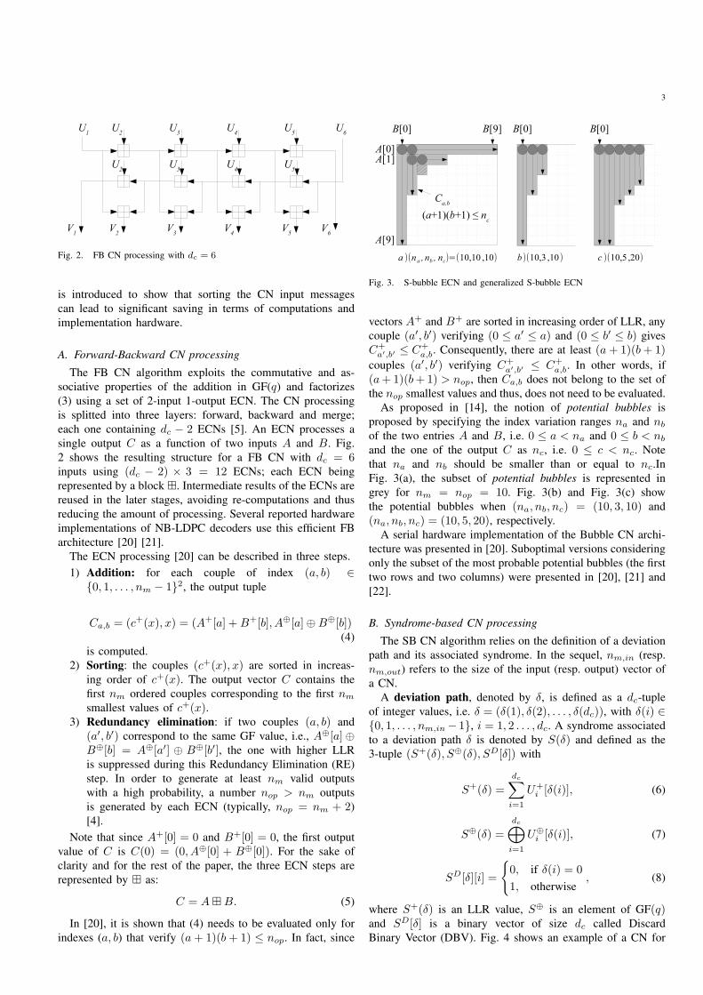
Fig. 2. FB CN processing with dc = 6

is introduced to show that sorting the CN input messages

can lead to significant saving in terms of computations and

implementation hardware.

A. Forward-Backward CN processing

The FB CN algorithm exploits the commutative and as-

sociative properties of the addition in GF(q) and factorizes

(3) using a set of 2-input 1-output ECN. The CN processing

is splitted into three layers: forward, backward and merge;

each one containing dc − 2 ECNs [5]. An ECN processes a

single output C as a function of two inputs A and B. Fig.

2 shows the resulting structure for a FB CN with dc = 6inputs using (dc − 2) × 3 = 12 ECNs; each ECN being

represented by a block ⊞. Intermediate results of the ECNs are

reused in the later stages, avoiding re-computations and thus

reducing the amount of processing. Several reported hardware

implementations of NB-LDPC decoders use this efficient FB

architecture [20] [21].

The ECN processing [20] can be described in three steps.

1) Addition: for each couple of index (a, b) ∈{0, 1, . . . , nm − 1}2, the output tuple

Ca,b = (c+(x), x) = (A+[a] +B+[b], A⊕[a]⊕B⊕[b])(4)

is computed.

2) Sorting: the couples (c+(x), x) are sorted in increas-

ing order of c+(x). The output vector C contains the

first nm ordered couples corresponding to the first nm

smallest values of c+(x).3) Redundancy elimination: if two couples (a, b) and

(a′, b′) correspond to the same GF value, i.e., A⊕[a]⊕B⊕[b] = A⊕[a′] ⊕ B⊕[b′], the one with higher LLR

is suppressed during this Redundancy Elimination (RE)

step. In order to generate at least nm valid outputs

with a high probability, a number nop > nm outputs

is generated by each ECN (typically, nop = nm + 2)

[4].

Note that since A+[0] = 0 and B+[0] = 0, the first output

value of C is C(0) = (0, A⊕[0] + B⊕[0]). For the sake of

clarity and for the rest of the paper, the three ECN steps are

represented by ⊞ as:

C = A⊞B. (5)

In [20], it is shown that (4) needs to be evaluated only for

indexes (a, b) that verify (a+ 1)(b+ 1) ≤ nop. In fact, since

Fig. 3. S-bubble ECN and generalized S-bubble ECN

vectors A+ and B+ are sorted in increasing order of LLR, any

couple (a′, b′) verifying (0 ≤ a′ ≤ a) and (0 ≤ b′ ≤ b) gives

C+a′,b′ ≤ C+

a,b. Consequently, there are at least (a+ 1)(b+ 1)

couples (a′, b′) verifying C+a′,b′ ≤ C+

a,b. In other words, if

(a+ 1)(b+ 1) > nop, then Ca,b does not belong to the set of

the nop smallest values and thus, does not need to be evaluated.

As proposed in [14], the notion of potential bubbles is

proposed by specifying the index variation ranges na and nb

of the two entries A and B, i.e. 0 ≤ a < na and 0 ≤ b < nb

and the one of the output C as nc, i.e. 0 ≤ c < nc. Note

that na and nb should be smaller than or equal to nc.In

Fig. 3(a), the subset of potential bubbles is represented in

grey for nm = nop = 10. Fig. 3(b) and Fig. 3(c) show

the potential bubbles when (na, nb, nc) = (10, 3, 10) and

(na, nb, nc) = (10, 5, 20), respectively.

A serial hardware implementation of the Bubble CN archi-

tecture was presented in [20]. Suboptimal versions considering

only the subset of the most probable potential bubbles (the first

two rows and two columns) were presented in [20], [21] and

[22].

B. Syndrome-based CN processing

The SB CN algorithm relies on the definition of a deviation

path and its associated syndrome. In the sequel, nm,in (resp.

nm,out) refers to the size of the input (resp. output) vector of

a CN.

A deviation path, denoted by δ, is defined as a dc-tuple

of integer values, i.e. δ = (δ(1), δ(2), . . . , δ(dc)), with δ(i) ∈{0, 1, . . . , nm,in− 1}, i = 1, 2 . . . , dc. A syndrome associated

to a deviation path δ is denoted by S(δ) and defined as the

3-tuple (S+(δ), S⊕(δ), SD[δ]) with

S+(δ) =

dc∑

i=1

U+i [δ(i)], (6)

S⊕(δ) =

dc⊕

i=1

U⊕i [δ(i)], (7)

SD[δ][i] =

{

0, if δ(i) = 0

1, otherwise, (8)

where S+(δ) is an LLR value, S⊕ is an element of GF(q)and SD[δ] is a binary vector of size dc called Discard

Binary Vector (DBV). Fig. 4 shows an example of a CN for

4

Fig. 4. Example of a deviation path

q = 64, dc = 4 and input messages Ui, i = 1, . . . , dc of size

nm,in = 5. In this figure, the deviation path δ = (0, 1, 0, 2)is represented by a grey shade in each input vector. It is also

represented with straight lines linking U1[0], U2[1], U3[0] and

U4[2]. Assuming that the elements of GF(64) are represented

by the power of a primitive element α, of GF(64) constructed

using the primitive polynomial P [α] = α6 + α + 1, the

syndrome associated to δ is S(δ) = (0 + 5 + 0 + 4, α56 ⊕α41 ⊕ α21 ⊕ α46, 0101) = (9, α42, 0101).

Let ∆0 be the set of all possible deviation paths that can

contribute to an output value, i.e., ∆0 ⊂ {0, . . . , nm,in−1}dc .

Using the syndrome associated to a deviation path, (3) can be

reformulated as

v+i (x) = minδ∈∆0,S⊕(δ)⊕U⊕

i[δ(i)]=x

{

S+(δ)− U+i [δ(i)]

}

. (9)

The DBV is used to reduce the complexity of (9) by

avoiding redundant computation. In fact, if SD[δ](i) = 0, then

δ(i) = 0 and U+i [δ(i)] = 0. It is thus possible to simplify (9)

and express it as

v+i (x) = minδ∈∆0,SD [δ][i]=0,S⊕(δ)⊕U⊕

i[0]=x

{

S+(δ)}

. (10)

Finally, (10) is further reduced by replacing δ ∈ ∆0 by

δ ∈ ∆ where ∆ is a subset of ∆0 with a reduced cardinality

|∆| = ns [10].

The SB CN algorithm proposed in [10] is summarized in

Algo. 1 and its associated architecture is presented in Fig.

5. Step 1 is performed by the Syndrome unit, Step 2 by the

Sorting unit and, finally, Step 3 by dc Decorrelation Units

(DU) and dc RE units. The DUs are represented in parallel

to show the inherent parallelism of the SB CN. The RE units

discard couples with a GF value already generated (last test

of step 3 in Algo. 1). Note that in [10], the sorting process is

done only partially.

Fig. 5 also shows a detailed scheme with the operations in

a DU. SD is the dc-wide bit vector that indicates for which

output edges the syndrome should be discarded during the

decorrelation process. A simple reading of bit i in the binary

vector SD validates or not the syndrome for the output edge

i.

C. Presorting of input messages

The idea of input presorting is to dynamically change

the order of inputs in the CN processor to classify reliable

Algorithm 1: The SB CN algorithm

Offline processing:

Select a subset ∆ ⊂ ∆0 of cardinality |∆| = ns.

Initialization:

for i← 1 to dc doji ← 0

end

Processing:

Step 1 (syndrome computation): ∀ δ ∈ ∆, compute S(δ)Step 2 (sorting process): sort the syndromes in the

increasing order of S+(δ) to obtain an ordered list

{S[k]}k=1,2,...,|∆| of syndromes;

Step 3 (decorrelation and RE):

for k ← 1 to |∆| do

for i← 1 to dc do

if SD[k][i] = 0 and ji < nm,out then

v⊕i ← S⊕[k]⊕ U⊕i [0]

if v⊕i /∈ {Vi[l]⊕}l=0...ji−1 then

Vi[ji]← (S+[k], v⊕i )ji ← ji + 1;

end

end

Fig. 5. Syndrome-based CN processing (left part) and details of the DU unit(right part).

and unreliable inputs. This polarization of the inputs makes

some deviation paths (for the SB CN [13]) or some potential

bubbles (for the FB CN [14]) very unlikely to contribute to an

output. The suppression of those useless configurations leads

to significant hardware saving without affecting performance.

The presorting principle, as described in Algorithm 2, can be

efficiently applied to the EMS algorithm [4] and their derived

implementations (FB CN [23][19] and SB CN [10]). Let us

consider the application of the presorting algorithm on the

EMS-based CN as illustrated in Fig. 6, where nm = 4 and

dc = 4. In this particular example, the hatched tuples represent

tuples that are not involved in the computation of the first

8 syndromes. Compared to the standard CN, the presorting

process requires extra hardware: a dc-input vector sorter and

two permutation networks (or switches). However, it allows

some simplifications in the CN itself, globally leading to an

important complexity reduction of the whole CN processing.

5

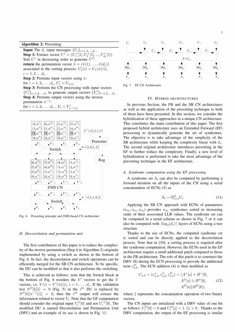
Algorithm 2: Presorting

Input The dc input messages {Ui}i=1,2,...,dc.

Step 1: Extract vector U1 = (U+1 [1], U+

2 [1], ..., U+dc[1])

Sort U1 in decreasing order to generate U ′1.

return the permutation vector π = (π(1), . . . , π(dc))associated to the sorting process: U ′

1(i) = U1(π(i)),i = 1, 2 . . . dc.

Step 2: Permute input vectors using π:

for i = 1, 2, . . . , dc, U ′i = Uπ(i)

Step 3: Perform the CN processing with input vectors

{U ′i}i=1,2,...,dc

to generate output vectors {V ′i }i=1,2,...,dc

.

Step 4: Permute output vectors using the inverse

permutation π−1:

for i = 1, 2, . . . , dc , Vi = V ′π−1(i)

Fig. 6. Presorting principle and EMS-based CN architecture

D. Decorrelation and permutation unit

The first contribution of this paper is to reduce the complex-

ity of the inverse permutation (Step 4 in Algorithm 2) originaly

implemented by using a switch as shown at the bottom of

Fig. 6. In fact, the decorrelation and switch operations can be

efficiently merged for the SB CN architecture. To be specific,

the DU can be modified so that it also performs the switching.

This is achieved as follows: note that the Switch block at

the bottom of Fig. 6 reorders the V ′ vectors to get the Vvectors, i.e. V (i) = V ′(π(i)), i = 1, . . . , dc. If the validation

test SD[k][i] = 0 (Fig. 5) in the ith DU is replaced by

SD[k][π−1(i)] = 0, then the ith output will extract the

information related to vector Vi. Note that the GF computation

should consider the original input U⊕i [0] and not U

′⊕i [0]. The

modified DU is named Decorrelation and Permutation Unit

(DPU) and an example of its use is shown in Fig. 11.

Fig. 7. EF CN Architecture

IV. HYBRID ARCHITECTURES

In previous Section, the FB and the SB CN architectures

as well as the application of the presorting technique to both

of them have been presented. In this section, we consider the

hybridization of these approaches in a unique CN architecture.

This constitutes the main contribution of this paper. The first

proposed hybrid architecture uses an Extended Forward (EF)

processing to dynamically generate the set of syndromes.

The objective is to take advantage of the simplicity of the

SB architecture while keeping the complexity linear with dc.

The second original architecture introduces presorting in the

EF to further reduce the complexity. Finally, a new level of

hybridization is performed to take the most advantage of the

presorting technique in the EF architecture.

A. Syndrome computation using the EF processing

A syndrome set Sb can also be computed by performing a

forward iteration on all the inputs of the CN using a serial

concatenation of ECNs (5) as

Sb = ⊞dc

i=1Ui. (11)

Applying the SB CN approach with ECNs of parameters

(nm, nm, nm) provides nm syndromes sorted in increasing

order of their associated LLR values. The syndrome set can

be computed in a serial scheme as shown in Fig. 7 or it can

also be computed with ⌈log2(dc)⌉ layers of ECNs using a tree

structure.

Thanks to the use of ECNs, the computed syndrome set

is sorted and can be directly applied to the decorrelation

process. Note that in [10], a sorting process is required after

the syndrome computation. However, the ECNs used in the EF

architecture require a small additional patch compared to those

in the FB architecture. The role of this patch is to construct the

DBV (8) during the ECN processing to provide the additional

term cDa,b. The ECN addition (4) is then modified as

Ca,b = (c+a,b, c⊕a,b, c

Da,b) = (A+[a] +B+[b],

A⊕[a]⊕B⊕[b],

AD[a]‖BD[b]),

(12)

where ‖ represents the concatenation operation of two binary

vectors.

The CN inputs are initialized with a DBV value of one bit

as follows: UDi [0] = 0 and UD

i [j] = 1, ∀j > 0 . Thanks to the

DBV computation, the output of the EF processing is similar

6

Fig. 8. Example to illustrate the redundant syndromes

to the output of the SB processing just before the decorrelation.

In particular, the notion of deviation path can be also applied

to the EF processing, with the only difference that the set of

deviation paths ∆EF is input dependent, while ∆ is predefined

offline in the SB architecture [10].

A first drawback of the EF is that the number of com-

puted syndromes is typically 3 × nm,out to compensate the

discarded redundant syndromes. Even with this approach, the

first simulation results of the EF algorithm showed significant

performance degradation compared to the FB algorithm [17].

The reason of this performance degradation resides in the

RE process performed by each ECN: since an ECN performs

RE, no more than one ECN output could be associated to a

given GF value. However, since the ECN outputs in the EF

algorithm are partial syndromes, RE may discard useful partial

syndromes that would construct valid complete syndromes

at the end of the EF processing. In Fig. 8, an example

of CN with dc = 4, nm,in = 2 and nm,out = 3 is

presented to illustrate the problem. The two deviation paths

δ1 = (1, 0, 0, 0) and δ2 = (0, 1, 0, 0) lead to the same GF

value, i.e., α4 + α0 + α4 + 0 = α0 + α4 + α4 + 0 = α0.

The output C1 = U1 ⊞ U2 of the first ECN is equal to

C1 = {(0, 0, 00), (1, α24, 10), (2, α24, 01), (3, 0, 11)} before

the RE and equal to C1 = {(0, 0, 00), (1, α24, 10)} af-

ter RE. Note that the seed of the partial syndrome δ2 is

eliminated. The final output in this example will be S =C3 = {(0, α4, 0000), (1, α0, 1000), (7, α17, 0010)} and after

the decorrelation unit, V1 = {(0, α24), (7, α47)}, instead of

V1 = {(0, α24), (2, 0), (7, α47)}. The key idea to avoid this

problem is to allow redundant GF values in the syndrome

set. Thus, removing the RE process from the ECN processing

avoids performance degradation. Let us define a modified

ECN operation with symbol ⊞′ where the ECN addition is

performed as in (12) and no RE is performed. The syndrome

set of size nm can then be computed as

S′b = ⊞

′dc

i=1Ui (13)

The RE process will then take place after the decorrelation

operation performed by the DUs. As previously mentioned, the

set of paths ∆ in the SB CN is pre-determined offline, while it

is determined dynamically on the fly in the EF CN according

to the current LLR values being processed. This leads to a

significant reduction of the total number ns of syndromes to

be computed.

B. EF CN with presorting

As shown in Section III-C, presorting leads to significant

hardware savings by reducing the number of candidate GF

symbols to be processed within the CN. In this section,

we show that this presorting technique, when applied to

the message vectors entering the EF CN, leads to a high

complexity reduction of the CN architecture. This architectural

reduction is obtained by reducing the number of bubbles to

be considered at each ECN. For this, we perform a statistical

study based on Monte-Carlo simulation that traces the paths

of the GF symbols that contribute to the output of the CN, in

their way across the different ECNs. This statistical study [14]

identifies in each ECN how often a given bubble contributes

to an output. This information allows pruning the bubbles

that never or rarely contribute. More formally, this study is

conducted through the following two steps:

1) Monte Carlo simulation giving the trace of the different

bubbles (each time a bubble b is used in an output

message, its score γ(b) is incremented).

2) ECN pruning that aims at discarding the less important

bubbles, thus simplifying the ECN architectures.

How to prune low-score bubbles for best efficiency is still an

open question. However, we propose here a method that prunes

bubbles based on the statistics of their scores at each ECN. Let

Ib be a sorted set of indexes of the potential bubbles of a given

ECN verifying ∀(b, b′) ∈ I2b , b < b′ ⇒ γ(b) ≤ γ(b′). Let τ be

a real between 0 and 1 and let Γ be the cumulative score of all

bubbles, i.e., Γ =∑

b∈Ibγ(b). The pruning process suppresses

the first p bubbles associated to the first p indexes of Ib, with

p defined as

p = arg maxp′∈Ib{

p′

∑

b=0

γ(b) ≤ τΓ}. (14)

After this pruning process, the structure of some ECNs is

greatly simplified. The choice of the values of τ is a trade-

off between hardware complexity and performance. As an

example, Fig. 9 represents the remaining bubbles after the

pruning process for a dc = 12 GF(64) (144, 120) NB-LDPC

code with nm,out set to 16. The pruning process has been

performed for an SNR of 5 dB and a value of τ equal to 0.01,

leading to different simplified ECN architectures:

• 1B: only a single bubble is considered where Ci is

given by C1 = {(0, U ′⊕1 [0] ⊕ U ′⊕

2 [0], 00)} and Ci ={(0, U ′⊕

i [0]⊕ C⊕i−1[0], C

Di−1[0]||0)} for i > 1.

• S-1B: it directly generates the nic sorted output Ci as

Ci = {(0, U′⊕i [0] ⊕ C⊕

i−1[0], CDi−1||0), (U

′+i [b], U ′⊕

i [b] ⊕C⊕

i−1[0], Ci−1||1)b=1...ni

b−1}. For this operation, a single

GF-adder is required.

• S-xB: with x > 1, also known as S-bubble ECN. As

described in [22], this architecture compares x bubbles

per clock cycle.

In Fig. 9, we represent each bubble in an ECN by a filled

circle and the direction for the next bubble by an arrow. The

size of the arrow is the size of the FIFO in the architecture.

Note that the complexity of the ECNs increases from left to

right. In fact, only trivial ECN blocks, i.e. 1B, S-1B, S-2B

architectures, are required on the left part while a S-5B ECN

is required on the right part. It is possible to regroup several

ECNs in a single component called Syndrome Node (SN). As

detailed hereafter, this SN computes sorted partial syndromes

7

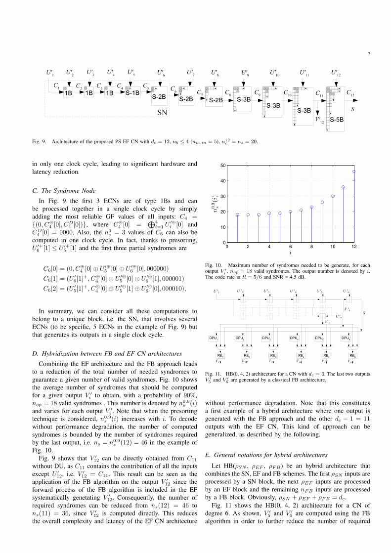
Fig. 9. Architecture of the proposed PS EF CN with dc = 12, nb ≤ 4 (nm,in = 5), n12c = ns = 20.

in only one clock cycle, leading to significant hardware and

latency reduction.

C. The Syndrome Node

In Fig. 9 the first 3 ECNs are of type 1Bs and can

be processed together in a single clock cycle by simply

adding the most reliable GF values of all inputs: C4 ={(0, C⊕

4 [0], CD4 [0])}, where C⊕

4 [0] =⊕4

i=1 U′⊕i [0] and

CD4 [0] = 0000. Also, the n6

c = 3 values of C6 can also be

computed in one clock cycle. In fact, thanks to presorting,

U ′+6 [1] ≤ U ′+

5 [1] and the first three partial syndromes are

C6[0] = (0, C⊕4 [0]⊕ U ′⊕

5 [0]⊕ U ′⊕6 [0], 000000)

C6[1] = (U ′6[1]

+, C⊕4 [0]⊕ U ′⊕

5 [0]⊕ U ′⊕6 [1], 000001)

C6[2] = (U ′5[1]

+, C⊕4 [0]⊕ U ′⊕

5 [1]⊕ U ′⊕6 [0], 000010),

In summary, we can consider all these computations to

belong to a unique block, i.e. the SN, that involves several

ECNs (to be specific, 5 ECNs in the example of Fig. 9) but

that generates its outputs in a single clock cycle.

D. Hybridization between FB and EF CN architectures

Combining the EF architecture and the FB approach leads

to a reduction of the total number of needed syndromes to

guarantee a given number of valid syndromes. Fig. 10 shows

the average number of syndromes that should be computed

for a given output V ′i to obtain, with a probability of 90%,

nop = 18 valid syndromes . This number is denoted by n0.9s (i)

and varies for each output V ′i . Note that when the presorting

technique is considered, n0.9s (i) increases with i. To decode

without performance degradation, the number of computed

syndromes is bounded by the number of syndromes required

by the last output, i.e. ns = n0.9s (12) = 46 in the example of

Fig. 10.

Fig. 9 shows that V ′12 can be directly obtained from C11

without DU, as C11 contains the contribution of all the inputs

except U ′12, i.e. V ′

12 = C11. This result can be seen as the

application of the FB algorithm on the output V ′12 since the

forward process of the FB algorithm is included in the EF

systematically genetating V ′12. Consequently, the number of

required syndromes can be reduced from ns(12) = 46 to

ns(11) = 36, since V ′12 is computed directly. This reduces

the overall complexity and latency of the EF CN architecture

0 2 4 6 8 10 120

10

20

30

40

50

i

n0.9

s(i)

Fig. 10. Maximum number of syndromes needed to be generate, for eachoutput V ′

i , nop = 18 valid syndromes. The output number is denoted by i.The code rate is R = 5/6 and SNR = 4.5 dB.

Fig. 11. HB(0, 4, 2) architecture for a CN with dc = 6. The last two outputsV ′

5and V ′

6are generated by a classical FB architecture.

without performance degradation. Note that this constitutes

a first example of a hybrid architecture where one output is

generated with the FB approach and the other dc − 1 = 11outputs with the EF CN. This kind of approach can be

generalized, as described by the following.

E. General notations for hybrid architectures

Let HB(ρSN , ρEF , ρFB) be an hybrid architecture that

combines the SN, EF and FB schemes. The first ρSN inputs are

processed by a SN block, the next ρEF inputs are processed

by an EF block and the remaining nFB inputs are processed

by a FB block. Obviously, ρSN + ρEF + ρFB = dc.

Fig. 11 shows the HB(0, 4, 2) architecture for a CN of

degree 6. As shown, V ′5 and V ′

6 are computed using the FB

algorithm in order to further reduce the number of required

8

syndromes. There are several possible HB architectures be-

tween the EF (i.e., HB(0, 6, 0)) and the classical FB CN

(i.e., HB(0, 0, 6)). Note that V ′6 (resp. V ′

5 ) should bypass the

decorrelation units and should be directly connected to Vπ(6)

(resp. Vπ(5)). Fig. 11 shows the case where π(6) = 3, i.e. the

third multiplexer connects V3 to V ′6 , and π(5) = 5, i.e. the

fifth multiplexer connects V5 to V ′6 . Finally, V1, V2, V4 and

V6 are each one connected to the output of the corresponding

DPU. Fig. 13 shows the HB(6, 4, 2) architecture for a CN of

degree 12. V ′11 and V ′

12 are computed using the FB algorithm

and a SN is used to process the 6 first input U ′1 to U ′

6.

F. Choice of parameters (ρSN , ρEF , ρFB)

The determination of the CN architecture parameters, i.e.

(ρSN , ρEF , ρFB) for the macro level, the internal structure of

the EF and the FB blocks (the parameters of each ECN) for

the micro level, is a complex problem. It can be formulated

as an optimization problem: how to minimize the hardware

complexity without introducing significant performance degra-

dation. In this paper, we have limited the value of ρFB to 1 and

2. Then, for the two hypotheses (0, dc − ρFB , ρFB)ρFB=1,2,

we have applied the same method than the one described in

Section IV-B to determine the parameters of each ECN of

the EF and FB blocks. Note that after the automatic raw

pruning process described in Section IV-B, the parameters

are further tuned by hand by a ”try and see (i.e. estimate

performance by simulation)” method. Once the pruning pro-

cess finished, the value of ρSN is fixed in order to optimize

the hardware efficiency of the CN architecture. In fact, at a

given point, CN with parameters (ρSN+1, ρEF −1, ρFB) will

have a higher hardware complexity than CN with parameters

(ρSN , ρEF , ρFB) but with a lower decoding latency.

G. Suppression of final output RE

In some decoder implementations [16] [20] with dv = 2,

the VNs connected to a CN are updated just after the CN

update. For example, in Fig. 11 a variable node unit may

be connected directly to each output V1 to V6 just after the

RE units RE1 to RE6. Also in some VN implementations

[16] [20], RE is performed in the VN. If this type of VN

is used, then the RE block can be removed from the hybrid

architecture for complexity reduction. The suppression of the

dc RE block is interesting specially for for high dc values. In

a HB architecture with final RE, the RE reduces the number

of output messages from ns (in case that all messages are

valid) to nm,out. Although removing the RE results in an

increase of the number of output messages (ns > nm,out),

it has a limited impact on the complexity since the nm,out

elements are processed on the fly by the VN, without the

need of intermediate storage. However, it may impact slightly

the VN power consumption since ns elements are processed

instead of nm,out. Note that the suppression of RE neither

affects the algorithm nor the performance since the RE is still

performed in the VN.

3 3.5 4 4.5 510

−8

10−7

10−6

10−5

10−4

10−3

10−2

10−1

100

Eb/N

o(dB)

FE

R

HB(6,6,0), nm

=16, ns=20

HB(6,5,1), nm

=16, ns=20

HB(6,4,2), nm

=16, ns=20

FB, nm

=16, nop

=18

Fig. 12. FER performance for a (144, 120) NB-LDPC code over GF(64).

Fig. 13. HB(6, 4, 2) architecture with dc = 12, nm,out = 16, nm,in = 5and ns = 20.

V. PERFORMANCE AND COMPLEXITY ANALYSIS

We consider GF(64)- and GF(256)-LDPC codes to obtain

performance and post-synthesis results for the different pro-

posed decoding architectures.

A. Performance

We ran bit-true Monte-Carlo simulations over the Addi-

tive White Gaussian Noise channel (AWGN) with a Binary

Phase Shift Keying (BPSK) modulation scheme. The different

parameters were set as follows: extrinsic and intrinsic LLR

messages quantified on 6 bits, the a posteriori LLRs on 7 bits

and the maximum number of decoding iterations to 10. The

matrices used in our simulations are available in [24].

Fig. 12 shows the obtained Frame Error Rate (FER) for

a GF(64) code of size (864,720) bits, code rate R = 5/6,

dc = 12 and dv = 2 over the Gaussian channel. We consider

the FB decoder in [22] as a reference, i.e. S-bubble algorithm

with 4 bubbles, nm = 16 and nop = 18. We simulated the

HB(6, 6, 0) or EF, the HB(6, 5, 1) and the HB(6, 4, 2)

architectures with the same number of computed syndromes

ns = 20. Fig. 13 shows the HB(6, 4, 2) architecture, for

which no performance degradation is observed. We observe

less than 0.05 dB of performance loss for the HB(6, 5, 1)

and around 0.2 dB for the HB(6, 6, 0) configuration. We

then conclude from these simulation results that the hybrid

architectures can achieve the same performance as the FB

9

3 3.5 4 4.510

−7

10−6

10−5

10−4

10−3

10−2

10−1

100

Eb/N

o(dB)

FE

R

HB(5,7,0), nm

=40, ns=50

HB(5,6,1), nm

=40, ns=50

HB(5,5,2), nm

=40, ns=50

FB nm

=40, nop

=45

Fig. 14. FER performance for a (144, 120) NB-LDPC code over GF(256).

3.2 3.4 3.6 3.8 4 4.210

−8

10−7

10−6

10−5

10−4

10−3

10−2

10−1

Eb/N

o(dB)

BE

R

T−MM

HB(10,5,1)

HB(10,4,2)

FB, nm

=16, nop

=18

Fig. 15. BER performance for a (1536, 1344) NB-LDPC code over GF(64).

architecture and outperform the EF architecture while needing

a reduced number of syndromes with a factor ranging from 3

to 4.

Fig. 14 shows performance results for a GF(256)-LDPC

code of size (1152, 960) bits, code rate R = 5/6, dc = 12and dv = 2. We consider as a reference the FB decoder with a

S-bubble architecture [22], 6 bubbles, nm = 40 and nop = 45.

The HB(5, 5, 2) architecture presents the same performance

as the FB and the HB(5, 6, 1) shows slight performance loss

smaller than 0.05 dB. The EF architecture presents around 0.1

dB of performance loss compared to the FB.

We can then conclude that this new family of hybrid

architectures allows for significant complexity reduction in CN

implementations without any performance loss compared to

more complex state-of-the-art solutions.

Fig. 15 shows performance results for a GF(64) (1536,

1344) LDPC code, code rate R = 7/8, dc = 16 and dv = 2.

As reference, we consider the FB decoder with a S-bubble

architecture [22], 4 bubbles, nm = 16 and nop = 18. The

architecture being used is the same as the one presented in

Fig. 13 except for the fact that the SN includes four more

TABLE IIPOST-SYNTHESIS RESULTS FOR DIFFERENT ECN ARCHITECTURES AND

CN SUB-UNITS ON 28 NM FD-SOI TECHNOLOGIE.

Area Power Pclk CL

(µm2) (mW) (ns) (cycles)

EC

Ns

1B 77 0.081 0.15 1S-1B 170 0.16 0.25 1S-2B 2570 1.66 0.79 1S-3B 3227 2.15 0.88 1S-4B 4022 2.57 1.03 1S-6B 5413 3.43 1.11 1

S-4B RE 4428 2.76 1.03 2S-6B RE 5818 3.64 1.11 2

CN

Su

b-u

nit

s 6-input SN 354 0.34 0.31 1PreSorter 12 1196 0.96 0.84 6PreSorter 16 1600 1.07 0.84 8

Switch 2724 1.95 0.28 1DPU 187 0.177 0.22 1RE 606 0.407 0.71 1

mult 64 107 0.070 0.34 1mult 256 178 1.082 0.43 1

1B ECNs (i.e., the HB(10, 4, 2) CN architecture). The T-

MM performance of a code of same length and coding rate

provided in [8] is also presented in Fig. 15. The Hybrid

architecture shows a performance gain of 0.5 dB over the T-

MM architecture. However, the performance gap may come

from the use of different parity check matrices. In [8] the

authors consider a dc = 24, dv = 3 code with an array

dispersion construction while we use a dc = 16, dv = 2 code

constructed using optimized coefficients for the parity checks

[25].

B. Implementation results

For complexity and power analysis, we considered the

implementation of the architectures on 28 nm FD-SOI tech-

nologies targeting a clock frequency of 800 MHz. The dif-

ferent kinds of ECNs presented in Fig. 9, were synthesized

individually to provide the results in Table II. Additionally,

the synthesis results of the SN, the S-bubble with RE (used

in the FB CN), the sorter, the switch, the DU (Fig. 5) and

the RE units implementation are also provided. The sorter is

implemented using a serial architecture as in [14], and the

switch is a cross bar switch. The minimum clock period (Pclk)

is given in nanoseconds with a clock uncertainty of 0.05 ns and

a setup time of 0.02 ns. The Cycle Latency (CL) represents

the number of clock cycles between the first input and the

first output. A reduction factor of 57, 34 and 7 is observed

betweeen the 1B and the S-4B RE architectures in terms

of area, power and clock period, respectively. These results

show that significant gain can be obtained thanks to ECN

simplification even if it implies the overcost of the presorter,

the switch and the DPU units.

Table III summarizes the implementation results for all the

CN architectures presented in this paper, for a GF(64) and a

GF(256)-LDPC codes with dc = 12. In this Table we present

the synthesis results with and without RE considering that the

RE can be suppressed in implementations when dv = 2 [16]

[20]. CL(CN) gives the latency in cycles between the first input

of a CN and the first output of a CN, taking into account the

latency of the ECNs, the Pre-Sorter, the switch, the DPU, the

10

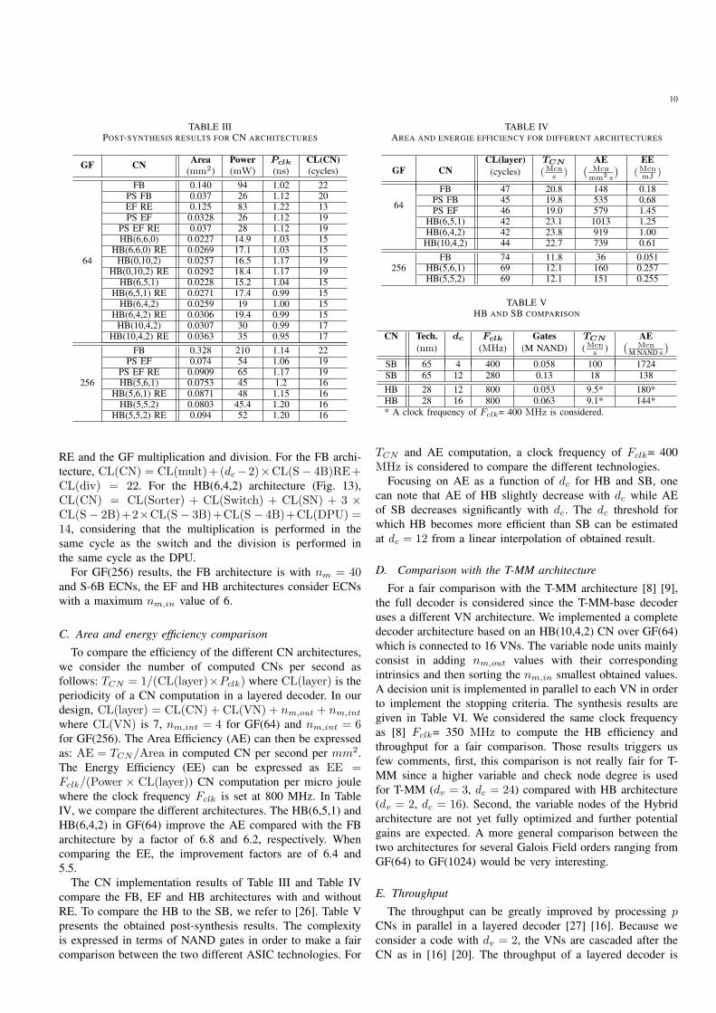
TABLE IIIPOST-SYNTHESIS RESULTS FOR CN ARCHITECTURES

GF CNArea Power Pclk CL(CN)

(mm2) (mW) (ns) (cycles)

64

FB 0.140 94 1.02 22PS FB 0.037 26 1.12 20EF RE 0.125 83 1.22 13PS EF 0.0328 26 1.12 19

PS EF RE 0.037 28 1.12 19HB(6,6,0) 0.0227 14.9 1.03 15

HB(6,6,0) RE 0.0269 17.1 1.03 15HB(0,10,2) 0.0257 16.5 1.17 19

HB(0,10,2) RE 0.0292 18.4 1.17 19HB(6,5,1) 0.0228 15.2 1.04 15

HB(6,5,1) RE 0.0271 17.4 0.99 15HB(6,4,2) 0.0259 19 1.00 15

HB(6,4,2) RE 0.0306 19.4 0.99 15HB(10,4,2) 0.0307 30 0.99 17

HB(10,4,2) RE 0.0363 35 0.95 17

256

FB 0.328 210 1.14 22PS EF 0.074 54 1.06 19

PS EF RE 0.0909 65 1.17 19HB(5,6,1) 0.0753 45 1.2 16

HB(5,6,1) RE 0.0871 48 1.15 16HB(5,5,2) 0.0803 45.4 1.20 16

HB(5,5,2) RE 0.094 52 1.20 16

RE and the GF multiplication and division. For the FB archi-

tecture, CL(CN) = CL(mult)+(dc−2)×CL(S− 4B)RE+CL(div) = 22. For the HB(6,4,2) architecture (Fig. 13),

CL(CN) = CL(Sorter) + CL(Switch) + CL(SN) + 3 ×CL(S− 2B)+2×CL(S− 3B)+CL(S− 4B)+CL(DPU) =14, considering that the multiplication is performed in the

same cycle as the switch and the division is performed in

the same cycle as the DPU.

For GF(256) results, the FB architecture is with nm = 40and S-6B ECNs, the EF and HB architectures consider ECNs

with a maximum nm,in value of 6.

C. Area and energy efficiency comparison

To compare the efficiency of the different CN architectures,

we consider the number of computed CNs per second as

follows: TCN = 1/(CL(layer)×Pclk) where CL(layer) is the

periodicity of a CN computation in a layered decoder. In our

design, CL(layer) = CL(CN) + CL(VN) + nm,out + nm,int

where CL(VN) is 7, nm,int = 4 for GF(64) and nm,int = 6for GF(256). The Area Efficiency (AE) can then be expressed

as: AE = TCN/Area in computed CN per second per mm2.

The Energy Efficiency (EE) can be expressed as EE =Fclk/(Power × CL(layer)) CN computation per micro joule

where the clock frequency Fclk is set at 800 MHz. In Table

IV, we compare the different architectures. The HB(6,5,1) and

HB(6,4,2) in GF(64) improve the AE compared with the FB

architecture by a factor of 6.8 and 6.2, respectively. When

comparing the EE, the improvement factors are of 6.4 and

5.5.

The CN implementation results of Table III and Table IV

compare the FB, EF and HB architectures with and without

RE. To compare the HB to the SB, we refer to [26]. Table V

presents the obtained post-synthesis results. The complexity

is expressed in terms of NAND gates in order to make a fair

comparison between the two different ASIC technologies. For

TABLE IVAREA AND ENERGIE EFFICIENCY FOR DIFFERENT ARCHITECTURES

GF CNCL(layer) TCN AE EE

(cycles) (Mcn

s)

(

Mcn

mm2s

)

(Mcn

mJ)

64

FB 47 20.8 148 0.18PS FB 45 19.8 535 0.68PS EF 46 19.0 579 1.45

HB(6,5,1) 42 23.1 1013 1.25HB(6,4,2) 42 23.8 919 1.00

HB(10,4,2) 44 22.7 739 0.61

256FB 74 11.8 36 0.051

HB(5,6,1) 69 12.1 160 0.257HB(5,5,2) 69 12.1 151 0.255

TABLE VHB AND SB COMPARISON

CN Tech. dc Fclk Gates TCN AE

(nm) (MHz) (M NAND) (Mcn

s)

(

Mcn

M NAND s

)

SB 65 4 400 0.058 100 1724

SB 65 12 280 0.13 18 138

HB 28 12 800 0.053 9.5* 180*

HB 28 16 800 0.063 9.1* 144*

* A clock frequency of Fclk= 400 MHz is considered.

TCN and AE computation, a clock frequency of Fclk= 400

MHz is considered to compare the different technologies.

Focusing on AE as a function of dc for HB and SB, one

can note that AE of HB slightly decrease with dc while AE

of SB decreases significantly with dc. The dc threshold for

which HB becomes more efficient than SB can be estimated

at dc = 12 from a linear interpolation of obtained result.

D. Comparison with the T-MM architecture

For a fair comparison with the T-MM architecture [8] [9],

the full decoder is considered since the T-MM-base decoder

uses a different VN architecture. We implemented a complete

decoder architecture based on an HB(10,4,2) CN over GF(64)

which is connected to 16 VNs. The variable node units mainly

consist in adding nm,out values with their corresponding

intrinsics and then sorting the nm,in smallest obtained values.

A decision unit is implemented in parallel to each VN in order

to implement the stopping criteria. The synthesis results are

given in Table VI. We considered the same clock frequency

as [8] Fclk= 350 MHz to compute the HB efficiency and

throughput for a fair comparison. Those results triggers us

few comments, first, this comparison is not really fair for T-

MM since a higher variable and check node degree is used

for T-MM (dv = 3, dc = 24) compared with HB architecture

(dv = 2, dc = 16). Second, the variable nodes of the Hybrid

architecture are not yet fully optimized and further potential

gains are expected. A more general comparison between the

two architectures for several Galois Field orders ranging from

GF(64) to GF(1024) would be very interesting.

E. Throughput

The throughput can be greatly improved by processing pCNs in parallel in a layered decoder [27] [16]. Because we

consider a code with dv = 2, the VNs are cascaded after the

CN as in [16] [20]. The throughput of a layered decoder is

11

TABLE VIPOST-SYNTHESIS RESULTS OF HB(10,4,2) DECODER FOR (1512,1323)

NB-LDPC CODE OVER GF(64)

T-MM [9] T-MM [8] HB(10,4,2)

Technologie (nm) 90 90 28

Fclk(MHz) 270 350 800

Gate count (M NAND) 2.09 2.99 1.0

Thoughput (Mbps) 1403 1231 267*

Efficiency (Mbps/M gates) 671 412 222*

* A clock frequency of Fclk= 350 MHz is considered.

given by T = (Nb × Fclk × p)/(M × CL(layer) × itavr)where itavr is the average number of iterations and Fclk is

fixed at 800 MHz. The layered GF(64) (1536, 1344) code

allows different parallelism options depending on the splitting

factor [28] (p = 2, 3, 4, 6, 8, 12, 16, 24, 32, 48, 96). With an

observed average number of iterations at SNR = 4.0 of 1.5

and a parallelism of 12, the throughput can reach 1.2 Gbps

with p = 2 and 7.3 Gbps with p = 12.

VI. CONCLUSION

This paper was dedicated to low-complexity implementa-

tions of CN processors in NB-LDPC decoders. We reviewed

the state-of-the-art architectures that consider the Extended

Min-Sum algorithm and introduced new approaches to reduce

the hardware complexity of the CN processors. We particularly

focused on the effect of the presorting technique and the

advantages of the Extended-Forward architecture. We then pre-

sented the hybrid architectures which combine the Extended-

Forward and the Forward-Backward approaches to signifi-

cantly reduce the total number of computed syndromes. The

post-synthesis results on 28 nm ASIC technology showed that

the area efficiency is improved by a factor of 6.2 without any

performance loss, or by a factor of 6.8 with a performance loss

of 0.04 dB compared with the Forward-Backward architecture.

REFERENCES

[1] R. Gallager, “Low-density parity-check codes,” Ph.D. dissertation, Cam-bridge, 1963.

[2] M. C. Davey and D. J. C. MacKay, “Low density parity check codes overGF(q),” in Information Theory Workshop, 1998, Jun 1998, pp. 70–71.

[3] S. Pfletschinger and D. Declercq, “Getting closer to MIMO capacitywith non-binary codes and spatial multiplexing,” in Global Telecommu-

nications Conference (GLOBECOM 2010), 2010 IEEE, Dec 2010, pp.1–5.

[4] D. Declercq and M. Fossorier, “Decoding algorithms for nonbinaryLDPC codes over GF(q),” IEEE Transactions on Communications,vol. 55, no. 4, pp. 633–643, April 2007.

[5] A. Voicila, D. Declercq, F. Verdier, M. Fossorier, and P. Urard, “Low-complexity decoding for non-binary LDPC codes in high order fields,”IEEE Transactions on Communications, vol. 58, no. 5, pp. 1365–1375,May 2010.

[6] E. Li, D. Declercq, and K. Gunnam, “Trellis-based extended Min-Sumalgorithm for non-binary LDPC codes and its hardware structure,” IEEE

Transactions on Communications, vol. 61, no. 7, pp. 2600–2611, July2013.

[7] J. O. Lacruz, F. Garcıa-Herrero, J. Valls, and D. Declercq, “Oneminimum only trellis decoder for non-binary low-density parity-checkcodes,” IEEE Transactions on Circuits and Systems I: Regular Papers,vol. 62, no. 1, pp. 177–184, Jan 2015.

[8] J. O. Lacruz, F. Garcıa-Herrero, M. J. Canet, and J. Valls, “Reduced-complexity nonbinary LDPC decoder for high-order Galois fields basedon trellis Min-Max algorithm,” IEEE Transactions on Very Large Scale

Integration (VLSI) Systems, vol. 24, no. 8, pp. 2643–2653, Aug 2016.

[9] H. P. Thi and H. Lee, “Basic-set trellis Min-Max decoder architecturefor nonbinary LDPC codes with high-order Galois fields,” IEEE Trans-

actions on Very Large Scale Integration (VLSI) Systems, vol. 26, no. 3,pp. 496–507, March 2018.

[10] P. Schlafer, N. Wehn, M. Alles, T. Lehnigk-Emden, and E. Boutillon,“Syndrome based check node processing of high order NB-LDPCdecoders,” in Telecommunications (ICT), 2015 22nd International Con-

ference on, April 2015, pp. 156–162.[11] P. Schlafer, V. Rybalkin, N. Wehn, M. Alles, T. Lehnigk-Emden, and

E. Boutillon, “A new architecture for high throughput, low latencyNB-LDPC check node processing,” in Personal, Indoor, and Mobile

Radio Communications (PIMRC), 2015 IEEE 26th Annual International

Symposium on, Aug 2015, pp. 1392–1397.[12] V. Rybalkin, P. Schlafer, and N. Wehn, “A new architecture for high

speed, low latency NB-LDPC check node processing for GF(256),” in2016 IEEE 83rd Vehicular Technology Conference (VTC Spring), May2016, pp. 1–5.

[13] C. Marchand and E. Boutillon, “NB-LDPC check node with pre-sortedinput,” in 9th International Symposium on Turbo Codes and Iterative

Information Processing (ISTC), Sept 2016, pp. 196–200.[14] H. Harb, C. Marchand, A. A. Ghouwayel, L. Conde-Canencia, and

E. Boutillon, “Pre-sorted forward-backward NB-LDPC check nodearchitecture,” in IEEE International Workshop on Signal Processing

Systems (SiPS), Oct 2016, pp. 142–147.[15] Y. L. Ueng, K. H. Liao, H. C. Chou, and C. J. Yang, “A high-throughput

trellis-based layered decoding architecture for non-binary LDPC codesusing max-log-QSPA,” IEEE Transactions on Signal Processing, vol. 61,no. 11, pp. 2940–2951, June 2013.

[16] C. L. Lin, S. W. Tu, C. L. Chen, H. C. Chang, and C. Y. Lee, “Anefficient decoder architecture for nonbinary LDPC codes with extendedmin-sum algorithm,” IEEE Transactions on Circuits and Systems II:

Express Briefs, vol. 63, no. 9, pp. 863–867, Sept 2016.[17] C. Marchand, H. Harb, E. Boutillon, A. Al Ghouwayel, and L. Conde-

Canencia, “Extended-forward architecture for simplified check nodeprocessing in NB-LDPC decoders,” in IEEE International Workshop on

Signal Processing Systems (SiPS), October 2017.[18] C. Poulliat, M. Fossorier, and D. Declercq, “Design of regular (2,dc)-

LDPC codes over GF(q) using their binary images,” IEEE Transactions

on Communications, vol. 56, no. 10, pp. 1626–1635, October 2008.[19] A. Voicila, D. Declercq, F. Verdier, M. Fossorier, and P. Urard, “Low-

complexity decoding for non-binary LDPC codes in high order fields,”IEEE Transactions on Communications, vol. 58, no. 5, pp. 1365–1375,May 2010.

[20] E. Boutillon, L. Conde-Canencia, and A. A. Ghouwayel, “Design of aGF(64)-LDPC decoder based on the EMS algorithm,” IEEE Transac-

tions on Circuits and Systems I: Regular Papers, vol. 60, no. 10, pp.2644–2656, Oct 2013.

[21] Y. S. Park, Y. Tao, and Z. Zhang, “A fully parallel nonbinary LDPCdecoder with fine-grained dynamic clock gating,” IEEE Journal of Solid-

State Circuits, vol. 50, no. 2, pp. 464–475, Feb 2015.[22] O. Abassi, L. Conde-Canencia, A. A. Ghouwayel, and E. Boutillon, “A

novel architecture for elementary-check-node processing in nonbinaryLDPC decoders,” IEEE Transactions on Circuits and Systems II: Express

Briefs, vol. 64, no. 2, pp. 136–140, Feb 2017.[23] H. Wymeersch, H. Steendam, and M. Moeneclaey, “Log-domain de-

coding of LDPC codes over GF(q),” in Communications, 2004 IEEE

International Conference on, vol. 2, June 2004, pp. 772–776 Vol.2.[24] UBS. (2018) Non Binary LDPC. [Online]. Available: http:

//www-labsticc.univ-ubs.fr/nb ldpc/[25] E.Boutillon, “Optimization of non binary parity check coefficients,”

IEEE Transactions on Information Theory, 2018, submitted. [Online].Available: https://arxiv.org/abs/1708.01761

[26] P. Schlafer, “Implementation aspects of binary and non-binary low-density parity-check decoders,” Ph.D. dissertation, Technische UniversittKaiserslautern, 2016.

[27] Y. L. Ueng, C. Y. Leong, C. J. Yang, C. C. Cheng, K. H. Liao, and S. W.Chen, “An efficient layered decoding architecture for nonbinary QC-LDPC codes,” IEEE Transactions on Circuits and Systems I: Regular

Papers, vol. 59, no. 2, pp. 385–398, Feb 2012.[28] C. Marchand, J. B. Dore, L. Conde-Canencia, and E. Boutillon, “Con-

flict resolution for pipelined layered LDPC decoders,” in 2009 IEEE

Workshop on Signal Processing Systems, Oct 2009, pp. 220–225.

12

Cedric Marchand was born in 1976, France. Hereceived his B.E. degree in electrical and electronicsengineering from the North East Wales Institute,Wrexhan, Wales, 1999, M.Sc. and Ph.D. degreesin electrical engineering from the Universite Eu-ropeenne de Bretagne in 2007 and 2011 respectively.From 2007 to 2011, he has been working with NXPSemiconductor France on the implementation of anLDPC decoder for the DVB-S2, -T2 and -C2 stan-dards. In 2012, he joined Universite Bretagne Sudas research engineer. His current research interests

include decoding architectures for error correcting codes and VLSI design.

Emmanuel Boutillon was born in Chatou, Francein 1966. He received the Engineering Diploma fromTelecom Paris Tech, Paris, France in 1990. In 1991,he worked as an assistant professor in the EcoleMultinationale Superieure des Telecommunicationsin Africa (Dakar). In 1992, he joined Telecom ParisTech as a research engineer where he conductedresearch in the field of VLSI for digital communi-cations. He obtained his Ph.D in 1995. In 1998, hespent a sabbatical year at the University of Toronto,Ontario, Canada. In 2000, he joined Universite Bre-

tagne Sud as a professor. He headed the LESTER lab from 2005 up to endof 2007 and the CACS department between 2008 up to 2015. He is currentlythe scientific advisor of the Lab-STICC. In 2011, he had a sabbatical yearat INICTEL-UNI, Lima (Peru). His research interests are on the interactionsbetween algorithm and architecture in the field of wireless communicationsand high speed signal processing. In particular, he works on Turbo Codes andLDPC decoders.

Hassan Harb was born in 1992, Lebanon. Hereceived the Master 2 degree in electronics andtelecommunications from the Lebanese University,Lebanon, Beirut, 2015. Currently he is a PhD studentin cooperation between Universite Bretagne Sud,Lorient, France and Lebanese University, Beirut,Lebanon. He is working on the correction codecalled NB-LDPC algorithm, design and implemen-tation.

Laura Conde-Canencia received Eng. Degree fromUniversidad Politcnica de Madrid, Spain, in 2000and Ph.D. from Telecom Bretagne, France, in 2004.Since 2006 she is with the Lab-STICC Laboratory inUniversite Bretagne Sud (UBS), France, where sheis currently an Associate Professor. She is a mem-ber of the Scientific Advisory Board of UBS anda member of the International Relations AdvisoryBoard. In 2006-2007, she worked on PN sequencesynchronization for Global Navigation Satellite Sys-tem receivers. Since 2008, her research has mainly

focused on error correcting codes for digital communications: Turbo-codes,binary and non-binary LDPC codes and Cortex codes. From 2013 she hasextended her research topics to neural coding and neuromorphic design. Since2016 she is an elected member of the ”Design and Implementation of SignalProcessing Systems” Technical Committee (IEEE Signal Processing society).In 2017-2018, she was a Fulbright Visiting Research Scholar at University ofCalifornia Los Angeles (UCLA). During this year she was co-funded by theEuropean Union with a PRESTIGE grant award or Marie Curie Fellowship.

Ali Al Ghouwayel received his B.E. degree inPhysics-Electronics in 2002 from the Lebanese Uni-versity, Beirut, his B.E. degree in Electronics Engi-neering and his M.S. Degree in Telecommunicationsin 2004 from the National School of Engineeringof Brest (ENIB), Brest, France, and his PhD inSignal Processing and Telecommunications in 2008from the High School of Electricity (Suplec) andUniversity of Rennes 1, Rennes, France. His re-search activities concerned Parametrization Studyfor Software Radio Systems. In 2008, He joined the

Lab-STICC laboratory in Lorient, France and worked as a Post-Doctoralresearcher on the European Project DAVINCI. In 2010, He joined theLebanese International University, in Beirut, Lebanon, as Assistant Professorin the Computer and Communication Engineering Department. His currentresearch interests include Study, Optimization, and Adequation Algorithm-Architecture for Hardware Implementation of Non-Binary LDPC decoders,and Design of Reconfigurable Ultra-Throughput Rate Architectures for 5GSystems.