Hubness-aware Classiﬁcation, Instance Selection and ...cs.bme.hu/~buza/pdfs/marussyHubness.pdf ·...

Hubness-aware Classification, Instance Selectionand Feature Construction: Survey andExtensions to Time-Series

Nenad Tomasev, Krisztian Buza, Kristof Marussy, and Piroska B. Kis

Abstract Time-series classification is the common denominator in many real-worldpattern recognition tasks. In the last decade, the simple nearest neighbor classifier,in combination with dynamic time warping (DTW) as distance measure, has beenshown to achieve surprisingly good overall results on time-series classification prob-lems. On the other hand, the presence of hubs, i.e., instances that are similar toexceptionally large number of other instances, has been shown to be one of the cru-cial properties of time-series data sets. To achieve high performance, the presenceof hubs should be taken into account for machine learning tasks related to time-series. In this chapter, we survey hubness-aware classification methods and instanceselection, and we propose to use selected instances for feature construction. Weprovide detailed description of the algorithms using uniform terminology and nota-tions. Many of the surveyed approaches were originally introduced for vector clas-sification, and their application to time-series data is novel, therefore, we provideexperimental results on large number of publicly available real-world time-seriesdata sets.

Key words: time series classification, hubs, instance selection, feature construction

Nenad TomasevInstitute Jozef Stefan, Artificial Intelligence Laboratory, Jamova 39, 1000 Ljubljana, Sloveniae-mail: [email protected]

Krisztian BuzaFaculty of Mathematics, Informatics and Mechanics, University of Warsaw (MIMUW), Banacha 2,02-097 Warszawa, Poland, e-mail: [email protected]

Kristof MarussyDepartment of Computer Science and Information Theory, Budapest University of Technology andEconomics, Magyar tudosok krt. 2., 1117 Budapest, Hungary, e-mail: [email protected]

Piroska B. KisDepartment of Mathematics and Computer Science, College of Dunaujvaros, Tancsics M. u. 1/a,2400 Dunaujvaros, Hungary, e-mail: [email protected]

1

2 Nenad Tomasev, Krisztian Buza, Kristof Marussy, and Piroska B. Kis

1 Introduction

Time-series classification is one of the core components of various real-world recog-nition systems, such as computer systems for speech and handwriting recognition,signature verification, sign-language recognition, detection of abnormalities in elec-trocardiograph signals, tools based on electroencephalograph (EEG) signals (“brainwaves”), i.e., spelling devices and EEG-controlled web browsers for paralyzed pa-tients, and systems for EEG-based person identification, see e.g. [34, 35, 37, 45].Due to the increasing interest in time-series classification, various approaches havebeen introduced including neural networks [26, 38], Bayesian networks [48], hid-den Markov models [29, 33, 39], genetic algorithms, support vector machines [14],methods based on random forests and generalized radial basis functions [5] as wellas frequent pattern mining [17], histograms of symbolic polynomials [18] and semi-supervised approaches [36]. However, one of the most surprising results states thatthe simple k-nearest neighbor (kNN) classifier using dynamic time warping (DTW)as distance measure is competitive (if not superior) to many other state-of-the-artmodels for several classification tasks, see e.g. [9] and the references therein. Be-sides experimental evidence, there are theoretical results about the optimality ofnearest neighbor classifiers, see e.g. [12]. Some of the recent theoretical works fo-cused on a time series classification, in particular on why nearest neighbor classifierswork well in case of time series data [10].

On the other hand, Radovanovic et al. observed the presence of hubs in time-series data, i.e., the phenomenon that a few instances tend to be the nearest neighborof surprisingly lot of other instances [43]. Furthermore, they introduced the notionof bad hubs. A hub is said to be bad if its class label differs from the class labels ofmany of those instances that have this hub as their nearest neighbor. In the context ofk-nearest neighbor classification, bad hubs were shown to be responsible for a largeportion of the misclassifications. Therefore, hubness-aware classifiers and instanceselection methods were developed in order to make classification faster and moreaccurate [8, 43, 50, 52, 53, 55].

As the presence of hubs is a general phenomenon characterizing many datasets,we argue that it is of relevance to feature selection approaches as well. Therefore,in this chapter, we will survey the aforementioned results and describe the most im-portant hubness-aware classifiers in detail using unified terminology and notations.As a first step towards hubness-aware feature selection, we will examine the usageof distances from the selected instances as features in a state-of-the-art classifier.

The methods proposed in [50, 52, 53] and [55] were originally designed forvector classification and they are novel to the domain of time-series classification.Therefore, we will provide experimental evidence supporting the claim that thesemethods can be effectively applied to the problem of time-series classification. Theusage of distances from selected instances as features can be seen as transformingthe time-series into a vector space. While the technique of projecting the data into anew space is widely used in classification, see e.g. support vector machines [7, 11]and principal component analysis [25], to our best knowledge, the particular proce-

Hubness-aware classification, instance selection and feature construction 3

dure we perform is novel in time-series classification, therefore, we will experimen-tally evaluate it and compare to state-of-the-art time-series classifiers.

The remainder of this chapter is organized as follows: in Sect. 2 we formallydefine the time-series classification problem, summarize the basic notation usedthroughout this chapter and shortly describe nearest neighbor classification. Sec-tion 3 is devoted to dynamic time warping, and Sect. 4 presents the hubness phe-nomenon. In Sect. 5 we describe state-of-the-art hubness-aware classifiers, followedby hubness-aware instance selection and feature construction approaches in Sect. 6.Finally, we conclude in Sect. 7.

2 Problem Formulation and Basic Notations

The problem of classification can be stated as follows. We are given a set of instancesand some groups. The groups are called classes, and they are denoted as C1, . . . ,Cm.Each instance x belongs to one of the classes.1 Whenever x belongs to class Ci, wesay that the class label of x is Ci. We denote the set of all the classes by C , i.e.,C = {C1, . . . ,Cm}. Let D be a dataset of instances xi and their class labels yi, i.e.,D = {(x1,y1) . . .(xn,yn)}. We are given a dataset D train, called training data. Thetask of classification is to induce a function f (x), called classifier, which is able toassign class labels to instances not contained in D train.

In real-world applications, for some instances we know (from measurementsand/or historical data) to which classes they belong, while the class labels of otherinstances are unknown. Based on the data with known classes, we induce a classifier,and use it to determine the class labels of the rest of the instances.

In experimental settings we usually aim at measuring the performance of a clas-sifier. Therefore, after inducing the classifier using D train, we use a second datasetD test , called test data: for the instances of D test , we compare the output of the clas-sifier, i.e., the predicted class labels, with the true class labels, and calculate the ac-curacy of classification. Therefore, the task of classification can be defined formallyas follows: given two datasets D train and D test , the task of classification is to inducea classifier f (x) that maximizes prediction accuracy for D test . For the induction off (x), however, solely D train can be used, but not D test .

Next, we describe the k-nearest neighbor classifier (kNN). Suppose, we are givenan instance x∗ ∈D test that should be classified. The kNN classifier searches for thosek instances of the training dataset that are most similar to x∗. These k most similarinstances are called the k nearest neighbors of x∗. The kNN classifier considers the knearest neighbors, and takes the majority vote of their labels and assigns this label tox∗: e.g. if k = 3 and two of the nearest neighbors of x∗ belong to class C1, while oneof the nearest neighbors of x belongs to class C2, then this 3-NN classifier recognizesx∗ as an instance belonging to the class C1.

1 In this chapter, we only consider the case when each instance belongs to exactly one class.Note, however, that the presence of hubs may be relevant in the context of multilabel and fuzzyclassification as well.


Table 1 Abbreviations used throughout the chapter and the sections where those concepts aredefined/explained.

Abbreviation Full name Definition

AKNN adaptive kNN Sect. 5.5BNk(x) bad k-occurrence of x Sect. 4DTW Dynamic Time Warping Sect. 3GNk(x) good k-occurrence of x Sect. 4h-FNN hubness-based fuzzy nearest neighbor Sect. 5.2HIKNN hubness information k-nearest neighbor Sect. 5.4hw-kNN hubness-aware weighting for kNN Sect. 5.1INSIGHT instance selection based on graph-coverage and Sect. 6.1

hubness for time-serieskNN k-nearest neighbor classifier Sect. 2NHBNN naive hubness Bayesian k-nearest Neighbor Sect. 5.3Nk(x) k-occurrence of x Sect. 4Nk,C(x) class-conditional k-occurrence of x Sect. 4SNk(x) skewness of Nk(x) Sect. 4RImb relative imbalance factor Sect. 5.5

We use Nk(x) to denote the set of k nearest neighbors of x. Nk(x) is also calledas the k-neighborhood of x.

3 Dynamic Time Warping

While the kNN classifier is intuitive in vector spaces, in principle, it can be appliedto any kind of data, i.e., not only in case if the instances correspond to points of avector space. The only requirement is that an appropriate distance measure is presentthat can be used to determine the most similar train instances. In case of time-seriesclassification, the instances are time-series and one of the most widely used distancemeasures is DTW. We proceed by describing DTW. We assume that a time-series xof length l is a sequence of real numbers: x = (x[0],x[1], . . . ,x[l −1]).

In the most simple case, while calculating the distance of two time series x1and x2, one would compare the k-th element of x1 to the k-th element of x2 andaggregate the results of such comparisons. In reality, however, when observing thesame phenomenon several times, we cannot expect it to happen (or any characteristicpattern to appear) always at exactly the same time position, and the event’s durationcan also vary slightly. Therefore, DTW captures the similarity of two time series’shapes in a way that it allows for elongations: the k-th position of time series x1 iscompared to the k′-th position of x2, and k′ may or may not be equal to k.

DTW is an edit distance [30]. This means that we can conceptually consider thecalculation of the DTW distance of two time series x1 and x2 of length l1 and l2respectively as the process of transforming x1 into x2. Suppose we have alreadytransformed a prefix (possibly having length zero or l1 in the extreme cases) of x1


1.1 2 5 5 3.8 2 1.3 0.8

0.75

2.3

4.1

4

1

3

2

x2

x1 Cost of

transforming

the marked

parts of x1

and x2.

Cost of transforming

the entire x1 into

the entire x2.

a)

1

2

3

4

5

6

7

8

9

10

11

12

13

14

15

16

17

18

19

20

21

22

23

...

...

...

The matrix

is filled in

this order.

b)

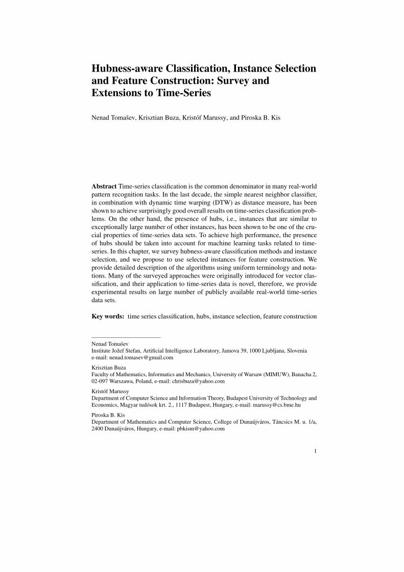
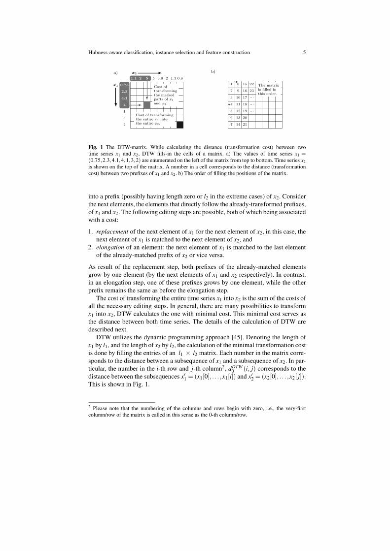
Fig. 1 The DTW-matrix. While calculating the distance (transformation cost) between twotime series x1 and x2, DTW fills-in the cells of a matrix. a) The values of time series x1 =(0.75,2.3,4.1,4,1,3,2) are enumerated on the left of the matrix from top to bottom. Time series x2is shown on the top of the matrix. A number in a cell corresponds to the distance (transformationcost) between two prefixes of x1 and x2. b) The order of filling the positions of the matrix.

into a prefix (possibly having length zero or l2 in the extreme cases) of x2. Considerthe next elements, the elements that directly follow the already-transformed prefixes,of x1 and x2. The following editing steps are possible, both of which being associatedwith a cost:

1. replacement of the next element of x1 for the next element of x2, in this case, thenext element of x1 is matched to the next element of x2, and

2. elongation of an element: the next element of x1 is matched to the last elementof the already-matched prefix of x2 or vice versa.

As result of the replacement step, both prefixes of the already-matched elementsgrow by one element (by the next elements of x1 and x2 respectively). In contrast,in an elongation step, one of these prefixes grows by one element, while the otherprefix remains the same as before the elongation step.

The cost of transforming the entire time series x1 into x2 is the sum of the costs ofall the necessary editing steps. In general, there are many possibilities to transformx1 into x2, DTW calculates the one with minimal cost. This minimal cost serves asthe distance between both time series. The details of the calculation of DTW aredescribed next.

DTW utilizes the dynamic programming approach [45]. Denoting the length ofx1 by l1, and the length of x2 by l2, the calculation of the minimal transformation costis done by filling the entries of an l1 × l2 matrix. Each number in the matrix corre-sponds to the distance between a subsequence of x1 and a subsequence of x2. In par-ticular, the number in the i-th row and j-th column2, dDTW

0 (i, j) corresponds to thedistance between the subsequences x′1 = (x1[0], . . . ,x1[i]) and x′2 = (x2[0], . . . ,x2[ j]).This is shown in Fig. 1.

2 Please note that the numbering of the columns and rows begin with zero, i.e., the very-firstcolumn/row of the matrix is called in this sense as the 0-th column/row.


1 1 3 4 3 1

1

2

3

3

4

1

0 0 2 5 7 7

1 1 1 3 4 5

3 3 1 2 2 4

5 5 1 2 2 4

8 8 2 1 2 5

8 8 4 4 3 2

x2

x1

a)

|3 − 3| + min{2, 3, 4} = 2

b)

1 1 3 4 3 1

1 2 3 3 4 1

c)

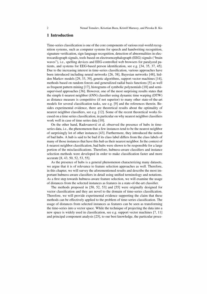
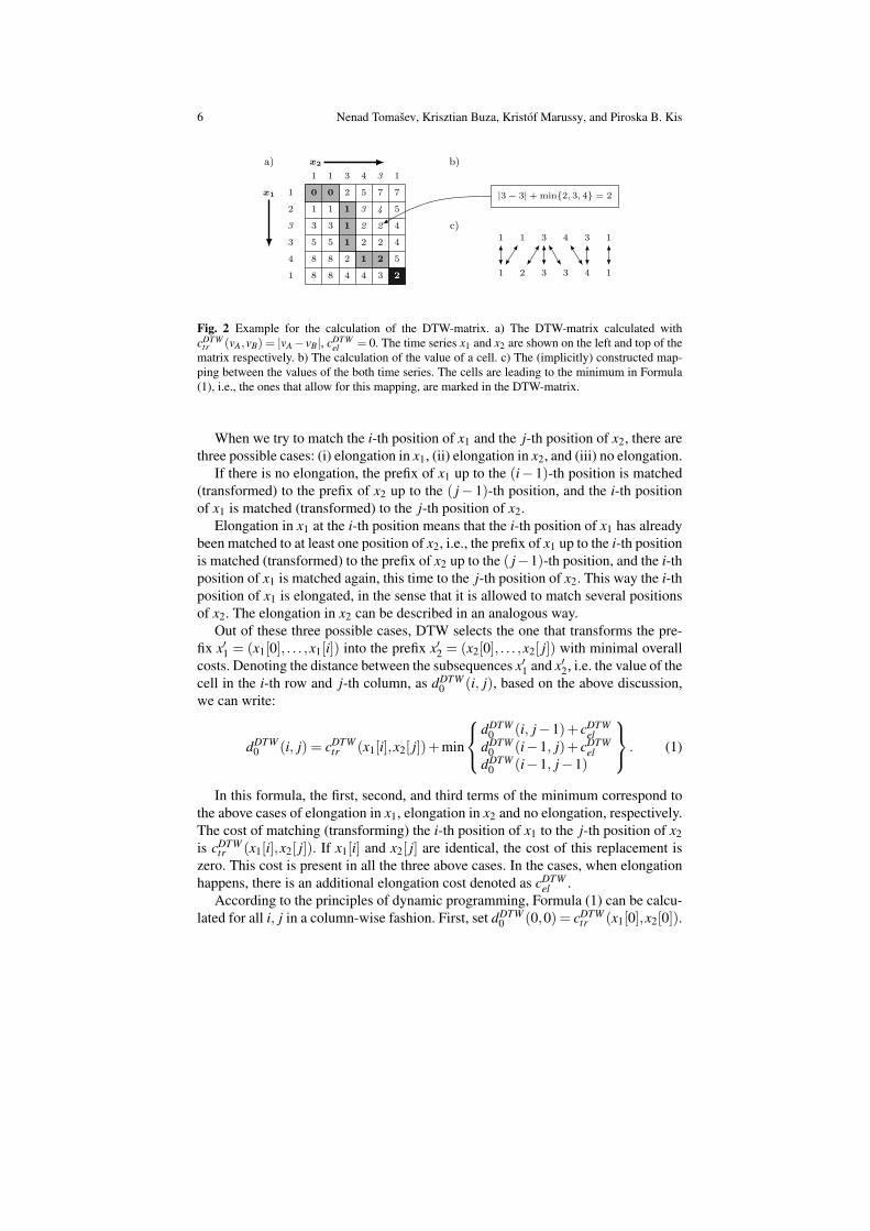
Fig. 2 Example for the calculation of the DTW-matrix. a) The DTW-matrix calculated withcDTW

tr (vA,vB) = |vA −vB|, cDTWel = 0. The time series x1 and x2 are shown on the left and top of the

matrix respectively. b) The calculation of the value of a cell. c) The (implicitly) constructed map-ping between the values of the both time series. The cells are leading to the minimum in Formula(1), i.e., the ones that allow for this mapping, are marked in the DTW-matrix.

When we try to match the i-th position of x1 and the j-th position of x2, there arethree possible cases: (i) elongation in x1, (ii) elongation in x2, and (iii) no elongation.

If there is no elongation, the prefix of x1 up to the (i−1)-th position is matched(transformed) to the prefix of x2 up to the ( j− 1)-th position, and the i-th positionof x1 is matched (transformed) to the j-th position of x2.

Elongation in x1 at the i-th position means that the i-th position of x1 has alreadybeen matched to at least one position of x2, i.e., the prefix of x1 up to the i-th positionis matched (transformed) to the prefix of x2 up to the ( j−1)-th position, and the i-thposition of x1 is matched again, this time to the j-th position of x2. This way the i-thposition of x1 is elongated, in the sense that it is allowed to match several positionsof x2. The elongation in x2 can be described in an analogous way.

Out of these three possible cases, DTW selects the one that transforms the pre-fix x′1 = (x1[0], . . . ,x1[i]) into the prefix x′2 = (x2[0], . . . ,x2[ j]) with minimal overallcosts. Denoting the distance between the subsequences x′1 and x′2, i.e. the value of thecell in the i-th row and j-th column, as dDTW

0 (i, j), based on the above discussion,we can write:

dDTW0 (i, j) = cDTW

tr (x1[i],x2[ j])+min

dDTW0 (i, j−1)+ cDTW

eldDTW

0 (i−1, j)+ cDTWel

dDTW0 (i−1, j−1)

. (1)

In this formula, the first, second, and third terms of the minimum correspond tothe above cases of elongation in x1, elongation in x2 and no elongation, respectively.The cost of matching (transforming) the i-th position of x1 to the j-th position of x2is cDTW

tr (x1[i],x2[ j]). If x1[i] and x2[ j] are identical, the cost of this replacement iszero. This cost is present in all the three above cases. In the cases, when elongationhappens, there is an additional elongation cost denoted as cDTW

el .According to the principles of dynamic programming, Formula (1) can be calcu-

lated for all i, j in a column-wise fashion. First, set dDTW0 (0,0) = cDTW

tr (x1[0],x2[0]).


Then we begin calculating the very first column of the matrix ( j = 0), followed bythe next column corresponding to j = 1, etc. The cells of each column are calculatedin order of their row-indexes: within one column, the cell in the row correspondingi = 0 is calculated first, followed by the cells corresponding to i = 1, i = 2, etc. (SeeFig. 1.) In some cases (in the very-first column and in the very-first cell of eachrow), in the min function of Formula (1), some of the terms are undefined (wheni−1 or j−1 equals −1). In these cases, the minimum of the other (defined) termsare taken.

The DTW distance of x1 and x2, i.e. the cost of transforming the entire time seriesx1 = (x1[0],x1[1], . . . ,x1[l1 −1]) into x2 = (x2[0],x2[1], . . . ,x2[l2 −1]) is

dDTW (x1,x2) = dDTW0 (l1 −1, l2 −1). (2)

An example for the calculation of DTW is shown in Fig. 2.Note that the described method implicitly constructs a mapping between the po-

sitions of the time series x1 and x2: by back-tracking which of the possible casesleads to the minimum in the Formula (1) in each step, i.e., which of the above dis-cussed three possible cases leads to the minimal transformation costs in each step,we can reconstruct the mapping of positions between x1 and x2.

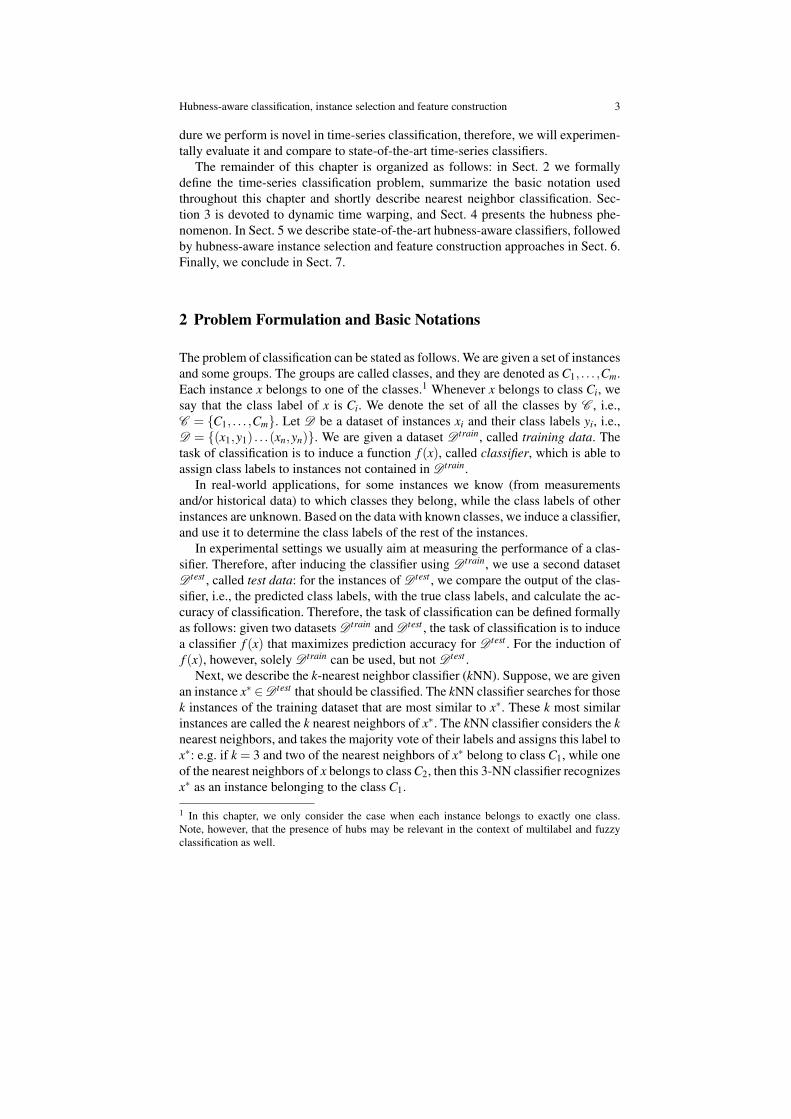
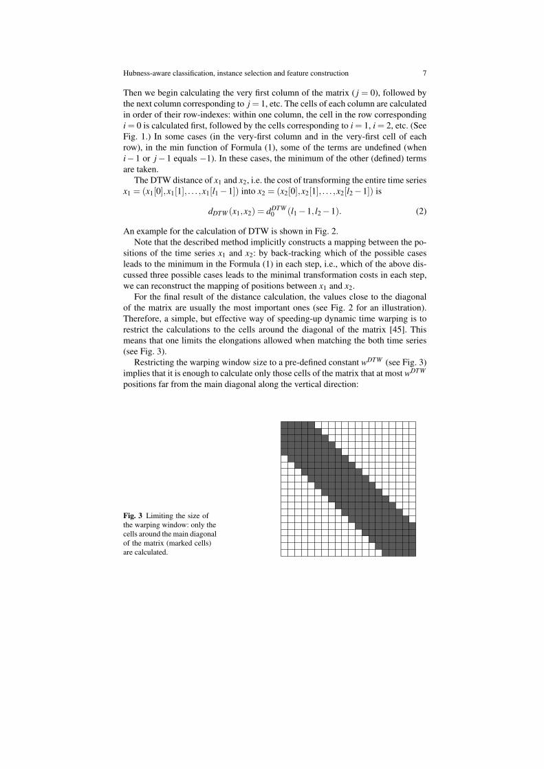
For the final result of the distance calculation, the values close to the diagonalof the matrix are usually the most important ones (see Fig. 2 for an illustration).Therefore, a simple, but effective way of speeding-up dynamic time warping is torestrict the calculations to the cells around the diagonal of the matrix [45]. Thismeans that one limits the elongations allowed when matching the both time series(see Fig. 3).

Restricting the warping window size to a pre-defined constant wDTW (see Fig. 3)implies that it is enough to calculate only those cells of the matrix that at most wDTW

positions far from the main diagonal along the vertical direction:

Fig. 3 Limiting the size ofthe warping window: only thecells around the main diagonalof the matrix (marked cells)are calculated.


dDTW0 (i, j) is calculated ⇔ |i− j| ≤ wDTW . (3)

The warping window size wDTW is often expressed in percentage relative to thelength of the time series. In this case, wDTW = 100% means calculating the entirematrix, while wDTW = 0% refers to the extreme case of not calculating any entries atall. Setting wDTW to a relatively small value such as 5%, does not negatively affectthe accuracy of the classification, see e.g. [9] and the references therein.

In the settings used throughout this chapter, the cost of elongation, cDTWel , is set

to zero:cDTW

el = 0. (4)

The cost of transformation (matching), denoted as cDTWtr , depends on what value is

replaced by what: if the numerical value vA is replaced by vB, the cost of this step is:

cDTWtr (vA,vB) = |vA − vB|. (5)

We set the warping window size to wDTW = 5%. For more details and further recentresults on DTW, we refer to [9].

4 Hubs in Time-Series Data

The presence of hubs, i.e., that some few instances tend to occur surprisingly fre-quently as nearest neighbors while other instances (almost) never occur as nearestneighbors, has been observed for various natural and artificial networks, such asprotein-protein-interaction networks or the internet [3, 22]. The presence of hubshas been confirmed in various contexts, including text mining, music retrieval andrecommendation, image data and time series [49, 46, 43]. In this chapter, we focuson time series classification, therefore, we describe hubness from the point of viewof time-series classification.

For classification, the property of hubness was explored in [40, 41, 42, 43]. Theproperty of hubness states that for data with high (intrinsic) dimensionality, likemost of the time series data3, some instances tend to become nearest neighbors muchmore frequently than others. Intuitively speaking, very frequent neighbors, or hubs,dominate the neighbor sets and therefore, in the context of similarity-based learning,they represent the centers of influence within the data. In contrast to hubs, there arerarely occurring neighbor instances contributing little to the analytic process. Wewill refer to them as orphans or anti-hubs.

In order to express hubness in a more precise way, for a time series dataset Done can define the k-occurrence of a time series x from D , denoted by Nk(x), as thenumber of time series in D having x among their k nearest neighbors:

Nk(x) = |{xi|x ∈ Nk(xi)}|. (6)

3 In case of time series, consecutive values are strongly interdependent, thus instead of the lengthof time series, we have to consider the intrinsic dimensionality [43].


CBF FacesUCRSonyAIBO

RobotSurface

0 2 4 6 8 10 12 14

100

200

300

400

500

0 1 2 3 4 5 6

200

400

600

800

0 1 2 3 4 5 6 7

100

200

300

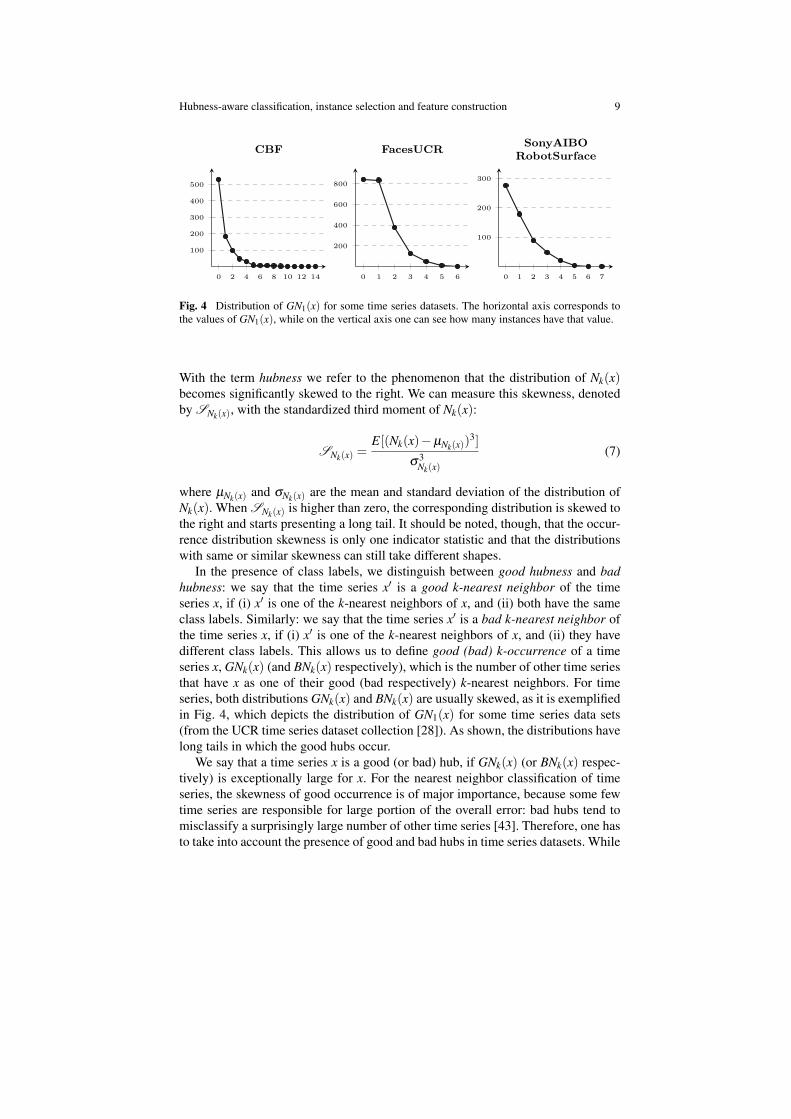
Fig. 4 Distribution of GN1(x) for some time series datasets. The horizontal axis corresponds tothe values of GN1(x), while on the vertical axis one can see how many instances have that value.

With the term hubness we refer to the phenomenon that the distribution of Nk(x)becomes significantly skewed to the right. We can measure this skewness, denotedby SNk(x), with the standardized third moment of Nk(x):

SNk(x) =E[(Nk(x)−µNk(x))

3]

σ3Nk(x)

(7)

where µNk(x) and σNk(x) are the mean and standard deviation of the distribution ofNk(x). When SNk(x) is higher than zero, the corresponding distribution is skewed tothe right and starts presenting a long tail. It should be noted, though, that the occur-rence distribution skewness is only one indicator statistic and that the distributionswith same or similar skewness can still take different shapes.

In the presence of class labels, we distinguish between good hubness and badhubness: we say that the time series x′ is a good k-nearest neighbor of the timeseries x, if (i) x′ is one of the k-nearest neighbors of x, and (ii) both have the sameclass labels. Similarly: we say that the time series x′ is a bad k-nearest neighbor ofthe time series x, if (i) x′ is one of the k-nearest neighbors of x, and (ii) they havedifferent class labels. This allows us to define good (bad) k-occurrence of a timeseries x, GNk(x) (and BNk(x) respectively), which is the number of other time seriesthat have x as one of their good (bad respectively) k-nearest neighbors. For timeseries, both distributions GNk(x) and BNk(x) are usually skewed, as it is exemplifiedin Fig. 4, which depicts the distribution of GN1(x) for some time series data sets(from the UCR time series dataset collection [28]). As shown, the distributions havelong tails in which the good hubs occur.

We say that a time series x is a good (or bad) hub, if GNk(x) (or BNk(x) respec-tively) is exceptionally large for x. For the nearest neighbor classification of timeseries, the skewness of good occurrence is of major importance, because some fewtime series are responsible for large portion of the overall error: bad hubs tend tomisclassify a surprisingly large number of other time series [43]. Therefore, one hasto take into account the presence of good and bad hubs in time series datasets. While


the kNN classifier is frequently used for time series classification, the k-nearestneighbor approach is also well suited for learning under class imbalance [21, 16, 20],therefore hubness-aware classifiers, the ones we present in the next section, are alsorelevant for the classification of imbalanced data.

The total occurrence count of an instance x can be decomposed into good and badoccurrence counts: Nk(x) = GNk(x)+BNk(x). More generally, we can decomposethe total occurrence count into the class-conditional counts: Nk(x) = ∑C∈C Nk,C(x)where Nk,C(x) denotes how many times x occurs as one of the k nearest neighborsof instances belonging to class C, i.e.,

Nk,C(x) = |{xi|x ∈ Nk(xi) ∧ yi =C}| (8)

where yi denotes the class label of xi.As we mentioned, hubs appear in data with high (intrinsic) dimensionality, there-

fore, hubness is one of the main aspects of the curse of dimensionality [4]. However,dimensionality reduction can not entirely eliminate the issue of bad hubs, unless itinduces significant information loss by reducing to a very low dimensional space -which often ends up hurting system performance even more [40].

5 Hubness-aware Classification of Time-Series

Since the issue of hubness in intrinsically high-dimensional data, such as time-series, can not be entirely avoided, the algorithms that work with high-dimensionaldata need to be able to properly handle hubs. Therefore, in this section, we presentalgorithms that work under the assumption of hubness. These mechanisms might beeither explicit or implicit.

Several hubness-aware classification methods have recently been proposed. Aninstance-weighting scheme was first proposed in [43], which reduces the bad influ-ence of hubs during voting. An extension of the fuzzy k-nearest neighbor frameworkwas shown to be somewhat better on average [53], introducing the concept of class-conditional hubness of neighbor points and building an occurrence model which isused in classification. This approach was further improved by considering the self-information of individual neighbor occurrences [50]. If the neighbor occurrences aretreated as random events, the Bayesian approaches also become possible [55, 52].

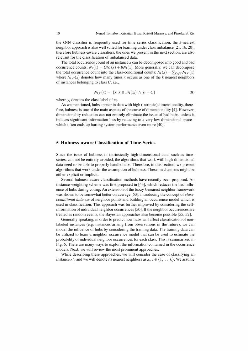
Generally speaking, in order to predict how hubs will affect classification of non-labeled instances (e.g. instances arising from observations in the future), we canmodel the influence of hubs by considering the training data. The training data canbe utilized to learn a neighbor occurrence model that can be used to estimate theprobability of individual neighbor occurrences for each class. This is summarized inFig. 5. There are many ways to exploit the information contained in the occurrencemodels. Next, we will review the most prominent approaches.

While describing these approaches, we will consider the case of classifying aninstance x∗, and we will denote its nearest neighbors as xi, i ∈ {1, . . . ,k}. We assume


Fig. 5 The hubness-aware analytic framework: learning from past neighbor occurrences.

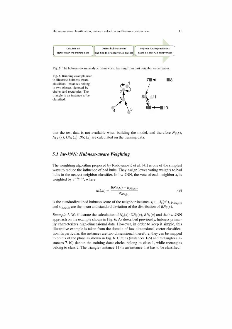
Fig. 6 Running example usedto illustrate hubness-awareclassifiers. Instances belongto two classes, denoted bycircles and rectangles. Thetriangle is an instance to beclassified.

that the test data is not available when building the model, and therefore Nk(x),Nk,C(x), GNk(x), BNk(x) are calculated on the training data.

5.1 hw-kNN: Hubness-aware Weighting

The weighting algorithm proposed by Radovanovic et al. [41] is one of the simplestways to reduce the influence of bad hubs. They assign lower voting weights to badhubs in the nearest neighbor classifier. In hw-kNN, the vote of each neighbor xi isweighted by e−hb(xi), where

hb(xi) =BNk(xi)−µBNk(x)

σBNk(x)(9)

is the standardized bad hubness score of the neighbor instance xi ∈ Nk(x∗), µBNk(x)and σBNk(x) are the mean and standard deviation of the distribution of BNk(x).

Example 1. We illustrate the calculation of Nk(x), GNk(x), BNk(x) and the hw-kNNapproach on the example shown in Fig. 6. As described previously, hubness primar-ily characterizes high-dimensional data. However, in order to keep it simple, thisillustrative example is taken from the domain of low dimensional vector classifica-tion. In particular, the instances are two-dimensional, therefore, they can be mappedto points of the plane as shown in Fig. 6. Circles (instances 1-6) and rectangles (in-stances 7-10) denote the training data: circles belong to class 1, while rectanglesbelong to class 2. The triangle (instance 11) is an instance that has to be classified.


Table 2 GN1(x), BN1(x), N1(x), N1,C1 (x) and N1,C2 (x) for the instances shown in Fig. 6.

Instance GN1(x) BN1(x) N1(x) N1,C1 (x) N1,C2 (x)

1 1 0 1 1 02 2 0 2 2 03 2 0 2 2 04 0 0 0 0 05 0 0 0 0 06 0 2 2 0 27 1 0 1 0 18 0 0 0 0 09 1 1 2 1 110 0 0 0 0 0

mean µGN1(x) = 0.7 µBN1(x) = 0.3 µN1(x) = 1std. σGN1(x) = 0.823 σBN1(x) = 0.675 σN1(x) = 0.943

For simplicity, we use k = 1 and we calculate N1(x), GN1(x) and BN1(x) for theinstances of the training data. For each training instance shown in Fig. 6, an arrowdenotes its nearest neighbor in the training data. Whenever an instance x′ is a goodneighbor of x, there is a continuous arrow from x to x′. In cases if x′ is a bad neighborof x, there is a dashed arrow from x to x′.

We can see, e.g., that instance 3 appears twice as good nearest neighbor of othertrain instances, while it never appears as bad nearest neighbor, therefore, GN1(x3) =2, BN1(x3) = 0 and N1(x3) =GN1(x3)+BN1(x3) = 2. For instance 6, the situation isthe opposite: GN1(x6)= 0, BN1(x6)= 2 and N1(x6)=GN1(x6)+BN1(x6)= 2, whileinstance 9 appears both as good and bad nearest neighbor: GN1(x9) = 1, BN1(x9) =1 and N1(x9) = GN1(x9)+BN1(x9) = 2. The second, third and fourth columns ofTable 2 show GN1(x), BN1(x) and N1(x) for each instance and the calculated meansand standard deviations of the distributions of GN1(x), BN1(x) and N1(x).

While calculating Nk(x), GNk(x) and BNk(x), we used k = 1. Note, however,that we do not necessarily have to use the same k for the kNN classification ofthe unlabeled/test instances. In fact, in case of kNN classification with k = 1, onlyone instance is taken into account for determining the class label, and therefore theweighting procedure described above does not make any difference to the simple 1nearest neighbor classification. In order to illustrate the use of the weighting proce-dure, we classify instance 11 with k′ = 2 nearest neighbor classifier, while Nk(x),GNk(x), BNk(x) were calculated using k = 1. The two nearest neighbors of instance11 are instances 6 and 9. The weights associated with these instances are:

w6 = e−hb(x6) = e−

BN1(x6)−µBN1(x)σBN1(x) = e−

2−0.30.675 = 0.0806 (10)

and

w9 = e−hb(x9) = e−

BN1(x9)−µBN1(x)σBN1(x) = e−

1−0.30.675 = 0.3545. (11)


As w9 > w6, instance 11 will be classified as rectangle according to instance 9.

From the example we can see that in hw-kNN all neighbors vote by their ownlabel. As this may be disadvantageous in some cases [49], in the algorithms consid-ered below, the neighbors do not always vote by thier own labels, which is a majordifference to hw-kNN.

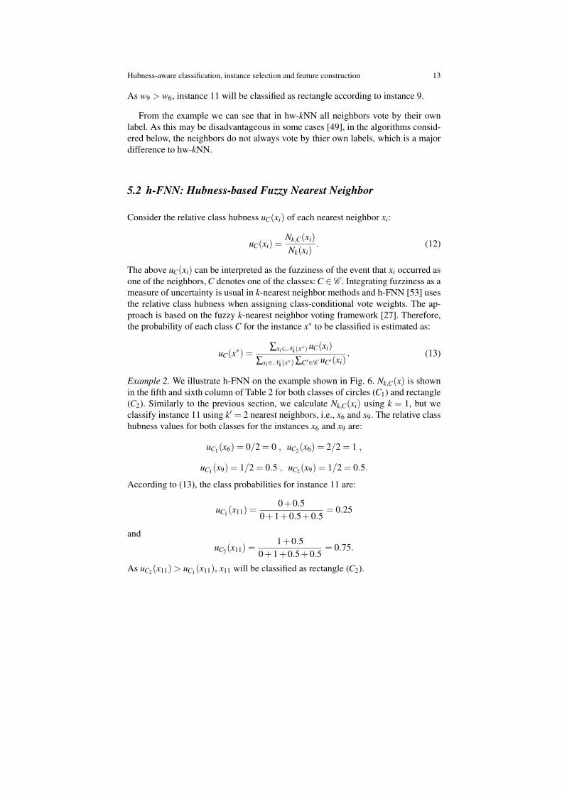
5.2 h-FNN: Hubness-based Fuzzy Nearest Neighbor

Consider the relative class hubness uC(xi) of each nearest neighbor xi:

uC(xi) =Nk,C(xi)

Nk(xi). (12)

The above uC(xi) can be interpreted as the fuzziness of the event that xi occurred asone of the neighbors, C denotes one of the classes: C ∈ C . Integrating fuzziness as ameasure of uncertainty is usual in k-nearest neighbor methods and h-FNN [53] usesthe relative class hubness when assigning class-conditional vote weights. The ap-proach is based on the fuzzy k-nearest neighbor voting framework [27]. Therefore,the probability of each class C for the instance x∗ to be classified is estimated as:

uC(x∗) =∑xi∈Nk(x∗) uC(xi)

∑xi∈Nk(x∗) ∑C′∈C uC′(xi). (13)

Example 2. We illustrate h-FNN on the example shown in Fig. 6. Nk,C(x) is shownin the fifth and sixth column of Table 2 for both classes of circles (C1) and rectangle(C2). Similarly to the previous section, we calculate Nk,C(xi) using k = 1, but weclassify instance 11 using k′ = 2 nearest neighbors, i.e., x6 and x9. The relative classhubness values for both classes for the instances x6 and x9 are:

uC1(x6) = 0/2 = 0 , uC2(x6) = 2/2 = 1 ,

uC1(x9) = 1/2 = 0.5 , uC2(x9) = 1/2 = 0.5.

According to (13), the class probabilities for instance 11 are:

uC1(x11) =0+0.5

0+1+0.5+0.5= 0.25

anduC2(x11) =

1+0.50+1+0.5+0.5

= 0.75.

As uC2(x11)> uC1(x11), x11 will be classified as rectangle (C2).


Special care has to be devoted to anti-hubs, such as instances 4 and 5 in Fig. 6.Their occurrence fuzziness is estimated as the average fuzziness of points from thesame class. Optional distance-based vote weighting is possible.

5.3 NHBNN: Naive Hubness Bayesian k-Nearest Neighbor

Each k-occurrence can be treated as a random event. What NHBNN [55] does isthat it essentially performs a Naive-Bayesian inference based on these k events

P(y∗ =C|Nk(x∗)) ∝ P(C) ∏xi∈Nk(x∗)

P(xi ∈ Nk|C). (14)

where P(C) denotes the probability that an instance belongs to class C and P(xi ∈Nk|C) denotes the probability that xi appears as one of the k nearest neighbors ofany instance belonging to class C. From the data, P(C) can be estimated as

P(C)≈|D train

C ||D train|

(15)

where |D trainC | denotes the number of train instances belonging to class C and |D train|

is the total number of train instances. P(xi ∈ Nk|C) can be estimated as the fraction

P(xi ∈ Nk|C)≈Nk,C(xi)

|D trainC |

. (16)

Example 3. Next, we illustrate NHBNN on the example shown in Fig. 6. Out of allthe 10 training instances, 6 belong to the class of circles (C1) and 4 belong to theclass of rectangles (C2). Therefore:

|D trainC1

|= 6 , |D trainC2

|= 4 , P(C1) = 0.6 , P(C2) = 0.4.

Similarly to the previous sections, we calculate Nk,C(xi) using k = 1, but we classifyinstance 11 using k′ = 2 nearest neighbors, i.e., x6 and x9. Thus, we calculate (16)for x6 and x9 for both classes C1 and C2:

P(x6 ∈ N1|C1)≈N1,C1(x6)

|D trainC1

|=

06= 0 , P(x6 ∈ N1|C2)≈

N1,C2(x6)

|D trainC2

|=

24= 0.5,

P(x9 ∈N1|C1)≈N1,C1(x9)

|D trainC1

|=

16= 0.167 , P(x9 ∈N1|C2)≈

N1,C2(x9)

|D trainC2

|=

14= 0.25 .

According to (14):

P(y11 =C1|N2(x11)) ∝ 0.6×0×0.167 = 0


P(y11 =C2|N2(x11)) ∝ 0.4×0.5×0.25 = 0.05

As P(y11 = C2|N2(x11)) > P(y11 = C1|N2(x11)), instance 11 will be classified asrectangle.

The previous example also illustrates that estimating P(xi ∈ Nk|C) according to(16) may simply lead zero probabilities. In order to avoid it, instead of (16), we canestimate P(xi ∈ Nk|C) as

P(xi ∈ Nk|C)≈ (1− ε)Nk,C(xi)

|D trainC |

+ ε (17)

where ε ≪ 1.Even though k-occurrences are highly correlated, NHBNN still offers some im-

provement over the basic kNN. It is known that the Naive Bayes rule can sometimesdeliver good results even in cases with high independence assumption violation [44].

Anti-hubs, i.e., instances that occur never or with an exceptionally low frequencyas nearest neighbors, are treated as a special case. For an anti-hub xi, P(xi ∈ Nk|C)can be estimated as the average of class-dependent occurrence probabilities of non-anti-hub instances belonging to the same class as xi:

P(xi ∈ Nk|C)≈ 1|D train

class(xi)| ∑

x j∈D trainclass(xi)

P(x j ∈ Nk|C). (18)

For more advanced techniques for the treatment of anti-hubs we refer to [55].

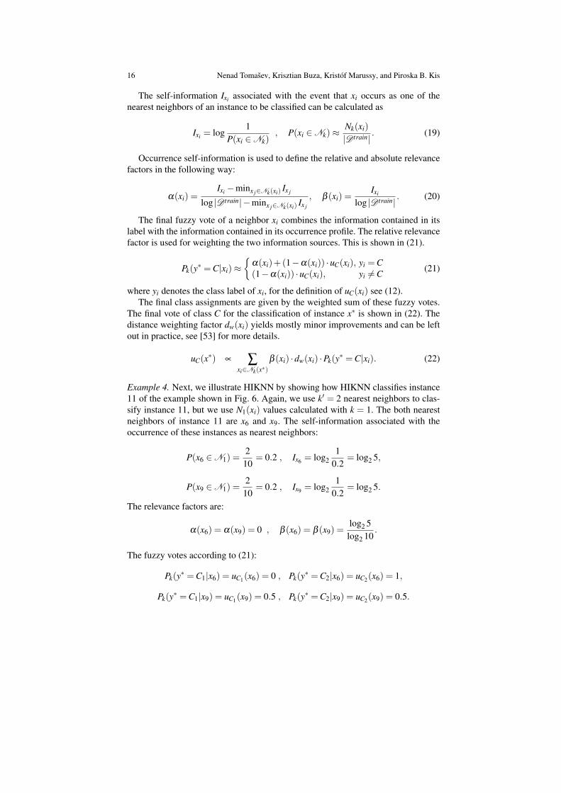
5.4 HIKNN: Hubness Information k-Nearest Neighbor

In h-FNN, as in most kNN classifiers, all neighbors are treated as equally important.The difference is sometimes made by introducing the dependency on the distanceto x∗, the instance to be classified. However, it is also possible to deduce some sortof global neighbor relevance, based on the occurrence model - and this is whatHIKNN was based on [50]. It embodies an information-theoretic interpretation ofthe neighbor occurrence events. In that context, rare occurrences have higher self-information, see (19). These more informative instances are favored by the algo-rithm. The reasons for this lie hidden in the geometry of high-dimensional featurespaces. Namely, hubs have been shown to lie closer to the cluster centers [54], asmost high-dimensional data lies approximately on hyper-spheres. Therefore, hubsare points that are somewhat less ’local’. Therefore, favoring the rarely occurringpoints helps in consolidating the neighbor set locality. The algorithm itself is a bitmore complex, as it not only reduces the vote weights based on the occurrence fre-quencies, but also modifies the fuzzy vote itself - so that the rarely occurring pointsvote mostly by their labels and the hub points vote mostly by their occurrence pro-files. Next, we will present the approach in more detail.


The self-information Ixi associated with the event that xi occurs as one of thenearest neighbors of an instance to be classified can be calculated as

Ixi = log1

P(xi ∈ Nk), P(xi ∈ Nk)≈

Nk(xi)

|D train|. (19)

Occurrence self-information is used to define the relative and absolute relevancefactors in the following way:

α(xi) =Ixi −minx j∈Nk(xi) Ix j

log |D train|−minx j∈Nk(xi) Ix j

, β (xi) =Ixi

log |D train|. (20)

The final fuzzy vote of a neighbor xi combines the information contained in itslabel with the information contained in its occurrence profile. The relative relevancefactor is used for weighting the two information sources. This is shown in (21).

Pk(y∗ =C|xi)≈{

α(xi)+(1−α(xi)) ·uC(xi), yi =C(1−α(xi)) ·uC(xi), yi =C (21)

where yi denotes the class label of xi, for the definition of uC(xi) see (12).The final class assignments are given by the weighted sum of these fuzzy votes.

The final vote of class C for the classification of instance x∗ is shown in (22). Thedistance weighting factor dw(xi) yields mostly minor improvements and can be leftout in practice, see [53] for more details.

uC(x∗) ∝ ∑xi∈Nk(x∗)

β (xi) ·dw(xi) ·Pk(y∗ =C|xi). (22)

Example 4. Next, we illustrate HIKNN by showing how HIKNN classifies instance11 of the example shown in Fig. 6. Again, we use k′ = 2 nearest neighbors to clas-sify instance 11, but we use N1(xi) values calculated with k = 1. The both nearestneighbors of instance 11 are x6 and x9. The self-information associated with theoccurrence of these instances as nearest neighbors:

P(x6 ∈ N1) =210

= 0.2 , Ix6 = log21

0.2= log2 5,

P(x9 ∈ N1) =210

= 0.2 , Ix9 = log21

0.2= log2 5.

The relevance factors are:

α(x6) = α(x9) = 0 , β (x6) = β (x9) =log2 5log2 10

.

The fuzzy votes according to (21):

Pk(y∗ =C1|x6) = uC1(x6) = 0 , Pk(y∗ =C2|x6) = uC2(x6) = 1,

Pk(y∗ =C1|x9) = uC1(x9) = 0.5 , Pk(y∗ =C2|x9) = uC2(x9) = 0.5.


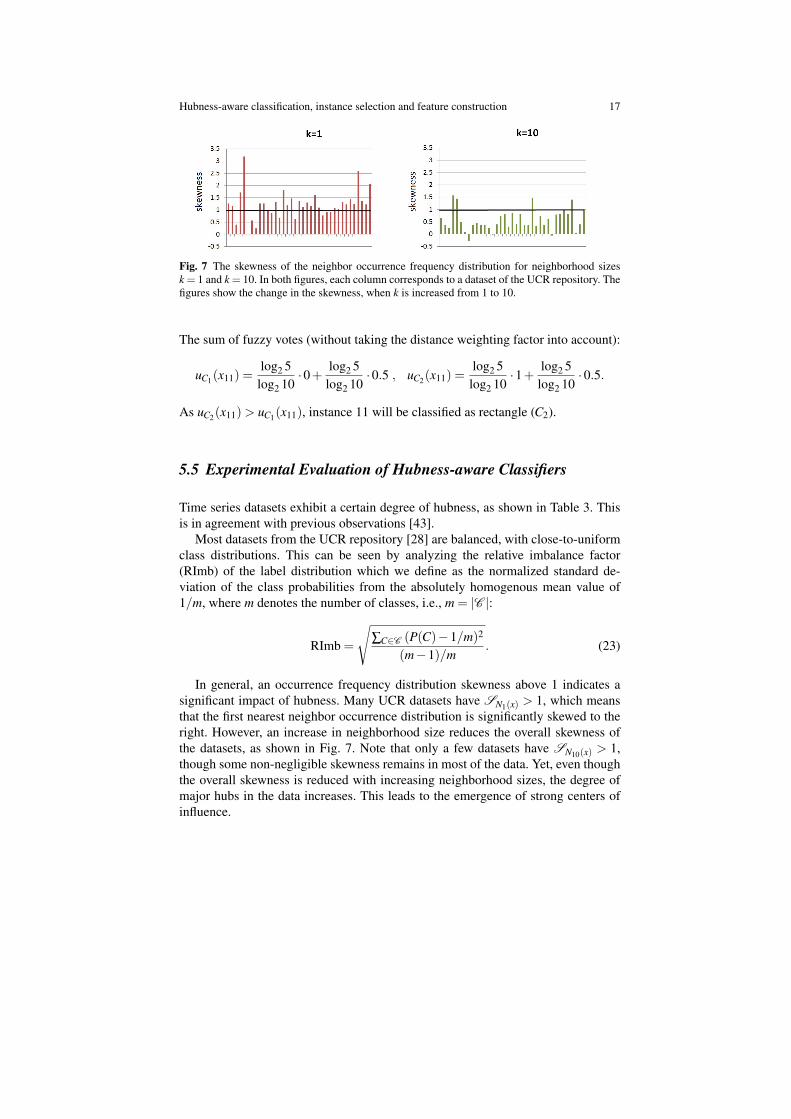
Fig. 7 The skewness of the neighbor occurrence frequency distribution for neighborhood sizesk = 1 and k = 10. In both figures, each column corresponds to a dataset of the UCR repository. Thefigures show the change in the skewness, when k is increased from 1 to 10.

The sum of fuzzy votes (without taking the distance weighting factor into account):

uC1(x11) =log2 5log2 10

·0+ log2 5log2 10

·0.5 , uC2(x11) =log2 5log2 10

·1+ log2 5log2 10

·0.5.

As uC2(x11)> uC1(x11), instance 11 will be classified as rectangle (C2).

5.5 Experimental Evaluation of Hubness-aware Classifiers

Time series datasets exhibit a certain degree of hubness, as shown in Table 3. Thisis in agreement with previous observations [43].

Most datasets from the UCR repository [28] are balanced, with close-to-uniformclass distributions. This can be seen by analyzing the relative imbalance factor(RImb) of the label distribution which we define as the normalized standard de-viation of the class probabilities from the absolutely homogenous mean value of1/m, where m denotes the number of classes, i.e., m = |C |:

RImb =

√∑C∈C (P(C)−1/m)2

(m−1)/m. (23)

In general, an occurrence frequency distribution skewness above 1 indicates asignificant impact of hubness. Many UCR datasets have SN1(x) > 1, which meansthat the first nearest neighbor occurrence distribution is significantly skewed to theright. However, an increase in neighborhood size reduces the overall skewness ofthe datasets, as shown in Fig. 7. Note that only a few datasets have SN10(x) > 1,though some non-negligible skewness remains in most of the data. Yet, even thoughthe overall skewness is reduced with increasing neighborhood sizes, the degree ofmajor hubs in the data increases. This leads to the emergence of strong centers ofinfluence.


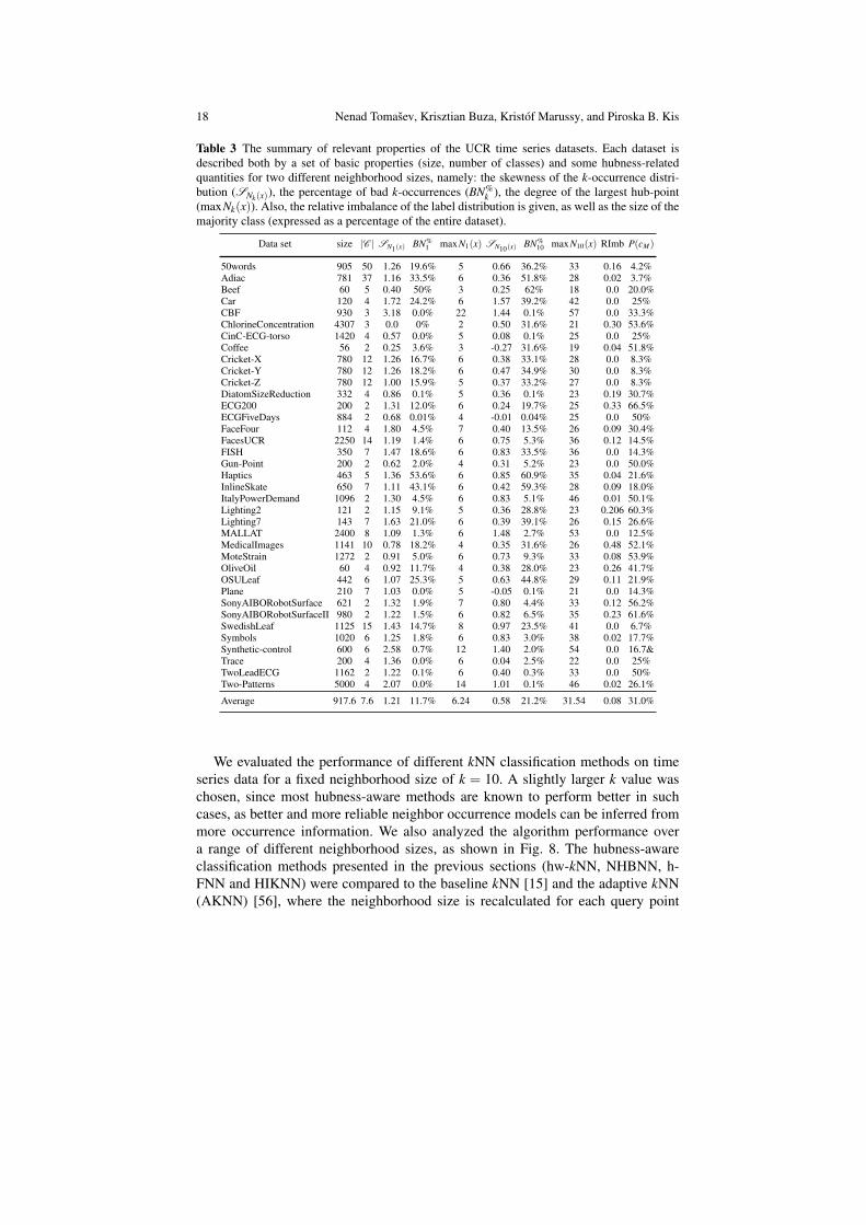
Table 3 The summary of relevant properties of the UCR time series datasets. Each dataset isdescribed both by a set of basic properties (size, number of classes) and some hubness-relatedquantities for two different neighborhood sizes, namely: the skewness of the k-occurrence distri-bution (SNk(x)), the percentage of bad k-occurrences (BN%

k ), the degree of the largest hub-point(maxNk(x)). Also, the relative imbalance of the label distribution is given, as well as the size of themajority class (expressed as a percentage of the entire dataset).

Data set size |C | SN1(x) BN%1 maxN1(x) SN10(x) BN%

10 maxN10(x) RImb P(cM)

50words 905 50 1.26 19.6% 5 0.66 36.2% 33 0.16 4.2%Adiac 781 37 1.16 33.5% 6 0.36 51.8% 28 0.02 3.7%Beef 60 5 0.40 50% 3 0.25 62% 18 0.0 20.0%Car 120 4 1.72 24.2% 6 1.57 39.2% 42 0.0 25%CBF 930 3 3.18 0.0% 22 1.44 0.1% 57 0.0 33.3%ChlorineConcentration 4307 3 0.0 0% 2 0.50 31.6% 21 0.30 53.6%CinC-ECG-torso 1420 4 0.57 0.0% 5 0.08 0.1% 25 0.0 25%Coffee 56 2 0.25 3.6% 3 -0.27 31.6% 19 0.04 51.8%Cricket-X 780 12 1.26 16.7% 6 0.38 33.1% 28 0.0 8.3%Cricket-Y 780 12 1.26 18.2% 6 0.47 34.9% 30 0.0 8.3%Cricket-Z 780 12 1.00 15.9% 5 0.37 33.2% 27 0.0 8.3%DiatomSizeReduction 332 4 0.86 0.1% 5 0.36 0.1% 23 0.19 30.7%ECG200 200 2 1.31 12.0% 6 0.24 19.7% 25 0.33 66.5%ECGFiveDays 884 2 0.68 0.01% 4 -0.01 0.04% 25 0.0 50%FaceFour 112 4 1.80 4.5% 7 0.40 13.5% 26 0.09 30.4%FacesUCR 2250 14 1.19 1.4% 6 0.75 5.3% 36 0.12 14.5%FISH 350 7 1.47 18.6% 6 0.83 33.5% 36 0.0 14.3%Gun-Point 200 2 0.62 2.0% 4 0.31 5.2% 23 0.0 50.0%Haptics 463 5 1.36 53.6% 6 0.85 60.9% 35 0.04 21.6%InlineSkate 650 7 1.11 43.1% 6 0.42 59.3% 28 0.09 18.0%ItalyPowerDemand 1096 2 1.30 4.5% 6 0.83 5.1% 46 0.01 50.1%Lighting2 121 2 1.15 9.1% 5 0.36 28.8% 23 0.206 60.3%Lighting7 143 7 1.63 21.0% 6 0.39 39.1% 26 0.15 26.6%MALLAT 2400 8 1.09 1.3% 6 1.48 2.7% 53 0.0 12.5%MedicalImages 1141 10 0.78 18.2% 4 0.35 31.6% 26 0.48 52.1%MoteStrain 1272 2 0.91 5.0% 6 0.73 9.3% 33 0.08 53.9%OliveOil 60 4 0.92 11.7% 4 0.38 28.0% 23 0.26 41.7%OSULeaf 442 6 1.07 25.3% 5 0.63 44.8% 29 0.11 21.9%Plane 210 7 1.03 0.0% 5 -0.05 0.1% 21 0.0 14.3%SonyAIBORobotSurface 621 2 1.32 1.9% 7 0.80 4.4% 33 0.12 56.2%SonyAIBORobotSurfaceII 980 2 1.22 1.5% 6 0.82 6.5% 35 0.23 61.6%SwedishLeaf 1125 15 1.43 14.7% 8 0.97 23.5% 41 0.0 6.7%Symbols 1020 6 1.25 1.8% 6 0.83 3.0% 38 0.02 17.7%Synthetic-control 600 6 2.58 0.7% 12 1.40 2.0% 54 0.0 16.7&Trace 200 4 1.36 0.0% 6 0.04 2.5% 22 0.0 25%TwoLeadECG 1162 2 1.22 0.1% 6 0.40 0.3% 33 0.0 50%Two-Patterns 5000 4 2.07 0.0% 14 1.01 0.1% 46 0.02 26.1%

Average 917.6 7.6 1.21 11.7% 6.24 0.58 21.2% 31.54 0.08 31.0%

We evaluated the performance of different kNN classification methods on timeseries data for a fixed neighborhood size of k = 10. A slightly larger k value waschosen, since most hubness-aware methods are known to perform better in suchcases, as better and more reliable neighbor occurrence models can be inferred frommore occurrence information. We also analyzed the algorithm performance overa range of different neighborhood sizes, as shown in Fig. 8. The hubness-awareclassification methods presented in the previous sections (hw-kNN, NHBNN, h-FNN and HIKNN) were compared to the baseline kNN [15] and the adaptive kNN(AKNN) [56], where the neighborhood size is recalculated for each query point


based on initial observations, in order to consult only the relevant neighbor points.AKNN does not take the hubness of the data into account.

The tests were run according to the 10-times 10-fold cross-validation proto-col and the statistical significance was determined by employing the corrected re-sampled t-test. The detailed results are given in Table 4.

The adaptive neighborhood approach (AKNN) does not seem to be appropriatefor handling time-series data, as it performs worse than the baseline kNN. Whilehw-kNN, NHBNN and h-FNN are better than the baseline kNN in some cases, theydo not offer significant advantage overall which is probably a consequence of arelatively low neighbor occurrence skewness for k = 10 (see Fig. 7). The hubnessis, on average, present in time-series data to a lower extent than in text or images [49]where these methods were previously shown to perform rather well.

On the other hand, HIKNN, the information-theoretic approach to handling vot-ing in high-dimensional data, clearly outperforms all other tested methods on thesetime series datasets. It performs significantly better than the baseline in 19 out of37 cases and does not perform significantly worse on any examined dataset. Its av-erage accuracy for k = 10 is 84.9, compared to 82.5 achieved by kNN. HIKNNoutperformed both baselines (even though not significantly) even in case of theChlorineConcentration dataset, which has very low hubness in terms of skewness,and therefore other hubness-aware classifiers worked worse than kNN on this data.These observations reaffirm the conclusions outlined in previous studies [50], ar-guing that HIKNN might be the best hubness-aware classifier on medium-to-lowhubness data, if there is no significant class imbalance. Note, however, that hubness-aware classifiers are also well suited for learning under class imbalance [16, 20, 21].

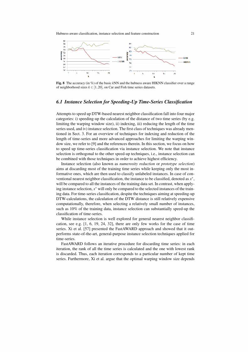
In order to show that the observed improvements are not merely an artifact ofthe choice of neighborhood size, classification tests were performed for a rangeof different neighborhood sizes. Figure 8 shows the comparisons between kNN andHIKNN for k ∈ [1,20], on Car and Fish time series datasets. There is little differencebetween kNN and HIKNN for k = 1 and the classifiers performance is similar inthis case. However, as k increases, so does the performance of HIKNN, while theperformance of kNN either decreases or increases at a slower rate. Therefore, thedifferences for k = 10 are more pronounced and the differences for k = 20 are evengreater. Most importantly, the highest achieved accuracy by HIKNN, over all testedneighborhoods, is clearly higher than the highest achieved accuracy by kNN.

These results indicate that HIKNN is an appropriate classification method forhandling time series data, when used in conjunction with the dynamic time warpingdistance.

Of course, choosing the optimal neighborhood size in k-nearest neighbor meth-ods is a non-trivial problem. The parameter could be set by performing cross-validation on the training data, though this is quite time-consuming. If the data issmall, using large k values might not make a lot of sense, as it would breach thelocality assumption by introducing neighbors into the kNN sets that are not relevantfor the instance to be classified. According to our experiments, HIKNN achievedvery good performance for k ∈ [5,15], therefore, setting k = 5 or k = 10 by defaultwould usually lead to reasonable results in practice.


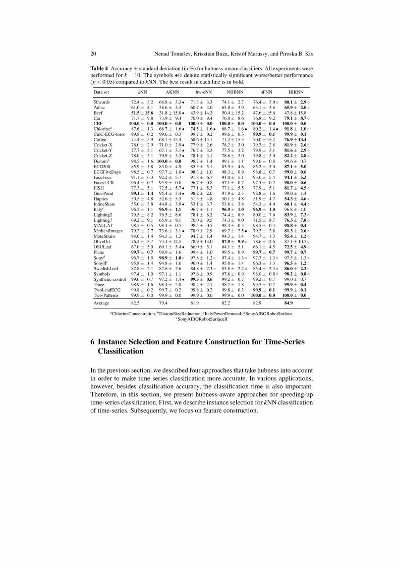
Table 4 Accuracy ± standard deviation (in %) for hubness-aware classifiers. All experiments wereperformed for k = 10. The symbols •/◦ denote statistically significant worse/better performance(p < 0.05) compared to kNN. The best result in each line is in bold.

Data set kNN AKNN hw-kNN NHBNN hFNN HIKNN

50words 72.4 ± 3.2 68.8 ± 3.3 • 71.3 ± 3.3 74.1 ± 2.7 76.4 ± 3.0 ◦ 80.1 ± 2.9 ◦Adiac 61.0 ± 4.1 58.6 ± 3.3 60.7 ± 4.0 63.8 ± 3.9 63.1 ± 3.8 65.9 ± 4.0 ◦Beef 51.5 ± 15.6 31.8 ± 15.0 • 43.9 ± 14.3 50.4 ± 15.2 47.6 ± 15.6 47.8 ± 15.8Car 71.7 ± 9.8 73.9 ± 9.4 76.0 ± 9.4 76.0 ± 8.6 76.8 ± 9.2 79.1 ± 8.7 ◦CBF 100.0 ± 0.0 100.0 ± 0.0 100.0 ± 0.0 100.0 ± 0.0 100.0 ± 0.0 100.0 ± 0.0Chlorinea 87.6 ± 1.3 68.7 ± 1.6 • 74.5 ± 1.6 • 68.7 ± 1.6 • 80.2 ± 1.4 • 91.8 ± 1.0 ◦CinC-ECG-torso 99.8 ± 0.2 99.6 ± 0.3 99.7 ± 0.2 99.6 ± 0.3 99.9 ± 0.1 99.9 ± 0.1Coffee 74.4 ± 15.9 68.7 ± 15.4 68.6 ± 15.1 71.2 ± 15.3 70.0 ± 15.2 76.9 ± 13.4Cricket-X 78.0 ± 2.9 71.0 ± 2.9 • 77.9 ± 2.6 78.2 ± 3.0 79.3 ± 2.8 81.9 ± 2.6 ◦Cricket-Y 77.7 ± 3.1 67.1 ± 3.1 • 76.7 ± 3.3 77.5 ± 3.2 79.9 ± 3.1 81.6 ± 2.9 ◦Cricket-Z 78.0 ± 3.1 70.9 ± 3.3 • 78.1 ± 3.1 78.6 ± 3.0 79.8 ± 3.0 82.2 ± 2.8 ◦Diatomb 98.5 ± 1.6 100.0 ± 0.0 98.7 ± 1.4 99.1 ± 1.1 99.6 ± 0.8 99.6 ± 0.7ECG200 85.9 ± 5.8 83.0 ± 4.9 85.3 ± 5.1 83.9 ± 4.6 85.2 ± 5.0 87.1 ± 5.0ECGFiveDays 98.5 ± 0.7 97.7 ± 1.0 • 98.3 ± 1.0 98.3 ± 0.9 98.8 ± 0.7 99.0 ± 0.6FaceFour 91.1 ± 6.3 92.2 ± 5.7 91.8 ± 6.7 94.0 ± 5.1 93.6 ± 5.4 94.1 ± 5.3FacesUCR 96.4 ± 0.7 95.9 ± 0.8 96.7 ± 0.8 97.1 ± 0.7 97.5 ± 0.7 98.0 ± 0.6FISH 77.3 ± 5.1 72.5 ± 5.7 • 77.1 ± 5.3 77.1 ± 5.5 77.9 ± 5.1 81.7 ± 4.5 ◦Gun-Point 99.1 ± 1.4 95.4 ± 3.4 • 98.2 ± 2.0 97.9 ± 2.3 98.8 ± 1.6 99.0 ± 1.4Haptics 50.5 ± 4.8 52.6 ± 5.5 51.3 ± 4.8 50.1 ± 4.8 51.9 ± 4.7 54.3 ± 4.6 ◦InlineSkate 55.0 ± 3.8 44.8 ± 3.9 • 53.1 ± 3.7 53.6 ± 3.8 54.3 ± 4.0 60.1 ± 4.4 ◦Italyc 96.5 ± 1.1 96.9 ± 1.1 96.7 ± 1.1 96.9 ± 1.0 96.9 ± 1.0 96.8 ± 1.0Lighting2 79.5 ± 8.2 76.5 ± 8.6 78.1 ± 8.2 74.4 ± 8.9 80.0 ± 7.6 83.9 ± 7.2 ◦Lighting7 69.2 ± 9.1 65.9 ± 9.1 70.0 ± 9.5 74.3 ± 9.0 71.5 ± 8.7 76.3 ± 7.8 ◦MALLAT 98.5 ± 0.5 98.4 ± 0.5 98.5 ± 0.5 98.4 ± 0.5 98.5 ± 0.4 98.8 ± 0.4MedicalImages 79.2 ± 2.7 73.6 ± 3.1 • 78.9 ± 2.9 69.2 ± 2.5 • 79.2 ± 2.8 81.3 ± 2.6 ◦MoteStrain 94.0 ± 1.4 94.3 ± 1.3 94.7 ± 1.4 94.3 ± 1.4 94.7 ± 1.3 95.4 ± 1.2 ◦OliveOil 76.2 ± 13.7 73.4 ± 12.5 78.9 ± 13.0 87.9 ± 9.9 ◦ 78.6 ± 12.6 87.1 ± 10.7 ◦OSULeaf 67.0 ± 5.0 60.1 ± 5.4 • 66.0 ± 5.1 64.1 ± 5.1 66.1 ± 4.5 72.5 ± 4.9 ◦Plane 99.7 ± 0.7 98.9 ± 1.6 99.4 ± 1.0 99.5 ± 0.9 99.7 ± 0.7 99.7 ± 0.7Sonyd 96.7 ± 1.5 98.9 ± 1.0 ◦ 97.8 ± 1.2 ◦ 97.4 ± 1.3 ◦ 97.7 ± 1.3 ◦ 97.5 ± 1.3 ◦SonyIIe 95.8 ± 1.4 94.8 ± 1.6 96.0 ± 1.4 95.8 ± 1.4 96.3 ± 1.3 96.5 ± 1.2SwedishLeaf 82.8 ± 2.1 82.6 ± 2.6 84.8 ± 2.3 ◦ 85.8 ± 2.2 ◦ 85.4 ± 2.3 ◦ 86.0 ± 2.2 ◦Symbols 97.4 ± 1.0 97.1 ± 1.1 97.6 ± 0.9 97.6 ± 0.9 98.0 ± 0.8 ◦ 98.2 ± 0.8 ◦Synthetic-control 99.0 ± 0.7 97.2 ± 1.4 • 99.5 ± 0.6 99.2 ± 0.7 99.2 ± 0.7 99.0 ± 0.7Trace 98.9 ± 1.6 98.4 ± 2.0 98.4 ± 2.1 98.7 ± 1.8 99.7 ± 0.7 99.9 ± 0.4TwoLeadECG 99.8 ± 0.2 99.7 ± 0.2 99.8 ± 0.2 99.8 ± 0.2 99.9 ± 0.1 99.9 ± 0.1Two-Patterns 99.9 ± 0.0 99.9 ± 0.0 99.9 ± 0.0 99.9 ± 0.0 100.0 ± 0.0 100.0 ± 0.0

Average 82.5 79.4 81.9 82.2 82.9 84.9

aChlorineConcentration, bDiatomSizeReduction, cItalyPowerDemand, d SonyAIBORobotSurface,eSonyAIBORobotSurfaceII

6 Instance Selection and Feature Construction for Time-SeriesClassification

In the previous section, we described four approaches that take hubness into accountin order to make time-series classification more accurate. In various applications,however, besides classification accuracy, the classification time is also important.Therefore, in this section, we present hubness-aware approaches for speeding-uptime-series classification. First, we describe instance selection for kNN classificationof time-series. Subsequently, we focus on feature construction.


Fig. 8 The accuracy (in %) of the basic kNN and the hubness aware HIKNN classifier over a rangeof neighborhood sizes k ∈ [1,20], on Car and Fish time series datasets.

6.1 Instance Selection for Speeding-Up Time-Series Classification

Attempts to speed up DTW-based nearest neighbor classification fall into four majorcategories: i) speeding-up the calculation of the distance of two time series (by e.g.limiting the warping window size), ii) indexing, iii) reducing the length of the timeseries used, and iv) instance selection. The first class of techniques was already men-tioned in Sect. 3. For an overview of techniques for indexing and reduction of thelength of time-series and more advanced approaches for limiting the warping win-dow size, we refer to [9] and the references therein. In this section, we focus on howto speed up time-series classification via instance selection. We note that instanceselection is orthogonal to the other speed-up techniques, i.e., instance selection canbe combined with those techniques in order to achieve highest efficiency.

Instance selection (also known as numerosity reduction or prototype selection)aims at discarding most of the training time series while keeping only the most in-formative ones, which are then used to classify unlabeled instances. In case of con-ventional nearest neighbor classification, the instance to be classified, denoted as x∗,will be compared to all the instances of the training data set. In contrast, when apply-ing instance selection, x∗ will only be compared to the selected instances of the train-ing data. For time-series classification, despite the techniques aiming at speeding-upDTW-calculations, the calculation of the DTW distance is still relatively expensivecomputationally, therefore, when selecting a relatively small number of instances,such as 10% of the training data, instance selection can substantially speed-up theclassification of time-series.

While instance selection is well explored for general nearest neighbor classifi-cation, see e.g. [1, 6, 19, 24, 32], there are only few works for the case of timeseries. Xi et al. [57] presented the FastAWARD approach and showed that it out-performs state-of-the-art, general-purpose instance selection techniques applied fortime-series.

FastAWARD follows an iterative procedure for discarding time series: in eachiteration, the rank of all the time series is calculated and the one with lowest rankis discarded. Thus, each iteration corresponds to a particular number of kept timeseries. Furthermore, Xi et al. argue that the optimal warping window size depends


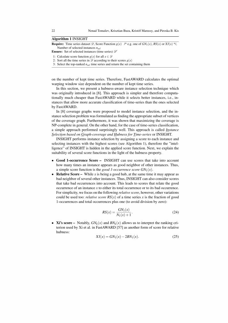
Algorithm 1 INSIGHTRequire: Time series dataset D , Score Function g(x) /* e.g. one of GN1(x), RS(x) or XI(x) */,

Number of selected instances nselEnsure: Set of selected instances (time series) D ′

1: Calculate score function g(x) for all x ∈ D2: Sort all the time series in D according to their scores g(x)3: Select the top-ranked nsel time series and return the set containing them

on the number of kept time series. Therefore, FastAWARD calculates the optimalwarping window size dependent on the number of kept time series.

In this section, we present a hubness-aware instance selection technique whichwas originally introduced in [8]. This approach is simpler and therefore computa-tionally much cheaper than FastAWARD while it selects better instances, i.e., in-stances that allow more accurate classification of time-series than the ones selectedby FastAWARD.

In [8] coverage graphs were proposed to model instance selection, and the in-stance selection problem was formulated as finding the appropriate subset of verticesof the coverage graph. Furthermore, it was shown that maximizing the coverage isNP-complete in general. On the other hand, for the case of time-series classification,a simple approach performed surprisingly well. This approach is called InstanceSelection based on Graph-coverage and Hubness for Time-series or INSIGHT.

INSIGHT performs instance selection by assigning a score to each instance andselecting instances with the highest scores (see Algorithm 1), therefore the ”intel-ligence” of INSIGHT is hidden in the applied score function. Next, we explain thesuitability of several score functions in the light of the hubness property.

• Good 1-occurrence Score – INSIGHT can use scores that take into accounthow many times an instance appears as good neighbor of other instances. Thus,a simple score function is the good 1-occurrence score GN1(x).

• Relative Score – While x is being a good hub, at the same time it may appear asbad neighbor of several other instances. Thus, INSIGHT can also consider scoresthat take bad occurrences into account. This leads to scores that relate the goodoccurrence of an instance x to either its total occurrence or to its bad occurrence.For simplicity, we focus on the following relative score, however, other variationscould be used too: relative score RS(x) of a time series x is the fraction of good1-occurrences and total occurrences plus one (to avoid division by zero):

RS(x) =GN1(x)

N1(x)+1. (24)

• Xi’s score – Notably, GNk(x) and BNk(x) allows us to interpret the ranking cri-terion used by Xi et al. in FastAWARD [57] as another form of score for relativehubness:

XI(x) = GN1(x)−2BN1(x). (25)


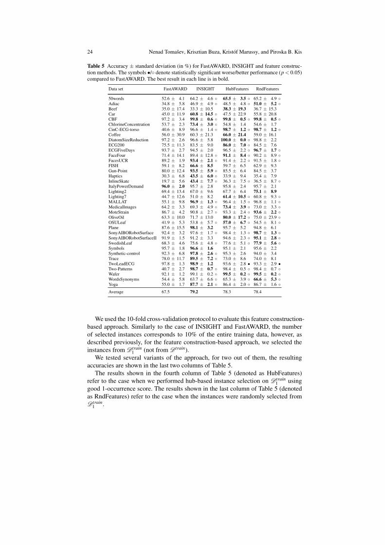
As reported in [8], INSIGHT outperforms FastAWARD both in terms of clas-sification accuracy and execution time. The second and third columns of Table 5present the average accuracy and corresponding standard deviation for each dataset, for the case when the number of selected instances is equal to 10% of the sizeof the training set. The experiments were performed according to the 10-fold cross-validation protocol. For INSIGHT, the good 1-occurrence score is used, but we notethat similar results were achieved for the other scores too.

In clear majority of the cases, INSIGHT substantially outperformed FastAWARD.In the few remaining cases, their difference are remarkably small (which are notsignificant in the light of the corresponding standard deviations). According to theanalysis reported in [8], one of the major reasons for the suboptimal performanceof FastAWARD is that the skewness degrades during the FastAWARD’s iterativeinstance selection procedure, and therefore FastAWARD is not able to select thebest instances in the end. This is crucial because FastAWARD discards the worstinstance in each iteration and therefore the final iterations have substantial impacton which instances remain, i.e., which instances will be selected by FastAWARD.

6.2 Feature Construction

As shown in Sect. 6.1, the instance selection approach focusing on good hubs leadsto overall good results. Previously, once the instances were selected, we simplyused them as training data for the kNN classifier. In a more advanced classificationschema, instead of simply performing nearest neighbor classification, we can usedistances from selected instances as features. This is described in detail below.

First, we split the training data D train into two disjoint subsets D train1 and D train

2 ,i.e., D train

1 ∩D train2 = /0, D train

1 ∪D train2 = D train. We select some instances from

D train1 , denote these selected instances as xsel,1,xsel,2, . . . ,xsel,l . For each instance

x ∈ D train2 , we calculate its DTW-distance from the selected instances and use these

distances as features of x. This way, we map each instance x ∈ D train2 into a vector

space:

xmapped =(dDTW (x,xsel,1),dDTW (x,xsel,2), . . . ,dDTW (x,xsel,l)

). (26)

The representation of the data in a vector space allows the usage of any conventionalclassifier. For our experiments, we trained logistic regression from the Weka soft-ware package4. We used the mapped instances of D train

2 as training data for logisticregression.

When classifying an instance x∗ ∈ D test , we map x∗ into the same vector spaceas the instances of D train

2 , i.e., we calculate the DTW-distances between x∗ and theselected instances xsel,1,xsel,2, . . . ,xsel,l and we use these distances as features ofx∗. Once the features of x∗ are calculated, we use the trained classifier (logisticregression in our case) to classify x∗.

4 http://www.cs.waikato.ac.nz/ml/weka/


Table 5 Accuracy ± standard deviation (in %) for FastAWARD, INSIGHT and feature construc-tion methods. The symbols •/◦ denote statistically significant worse/better performance (p < 0.05)compared to FastAWARD. The best result in each line is in bold.

Data set FastAWARD INSIGHT HubFeatures RndFeatures

50words 52.6 ± 4.1 64.2 ± 4.6 ◦ 65.5 ± 3.5 ◦ 65.2 ± 4.9 ◦Adiac 34.8 ± 5.8 46.9 ± 4.9 ◦ 48.5 ± 4.8 ◦ 51.0 ± 5.2 ◦Beef 35.0 ± 17.4 33.3 ± 10.5 38.3 ± 19.3 36.7 ± 15.3Car 45.0 ± 11.9 60.8 ± 14.5 ◦ 47.5 ± 22.9 55.8 ± 20.8CBF 97.2 ± 3.4 99.8 ± 0.6 ◦ 99.8 ± 0.5 ◦ 99.8 ± 0.5 ◦ChlorineConcentration 53.7 ± 2.3 73.4 ± 3.0 ◦ 54.8 ± 1.4 54.6 ± 1.7CinC-ECG-torso 40.6 ± 8.9 96.6 ± 1.4 ◦ 98.7 ± 1.2 ◦ 98.7 ± 1.2 ◦Coffee 56.0 ± 30.9 60.3 ± 21.3 66.0 ± 21.4 59.0 ± 16.1DiatomSizeReduction 97.2 ± 2.6 96.6 ± 5.8 100.0 ± 0.0 ◦ 98.8 ± 2.2ECG200 75.5 ± 11.3 83.5 ± 9.0 86.0 ± 7.0 ◦ 84.5 ± 7.6ECGFiveDays 93.7 ± 2.7 94.5 ± 2.0 96.5 ± 2.2 ◦ 96.7 ± 1.7 ◦FaceFour 71.4 ± 14.1 89.4 ± 12.8 ◦ 91.1 ± 8.4 ◦ 90.2 ± 8.9 ◦FacesUCR 89.2 ± 1.9 93.4 ± 2.1 ◦ 91.4 ± 2.2 ◦ 91.5 ± 1.8 ◦FISH 59.1 ± 8.2 66.6 ± 8.5 59.7 ± 6.5 62.9 ± 9.3Gun-Point 80.0 ± 12.4 93.5 ± 5.9 ◦ 85.5 ± 6.4 84.5 ± 3.7Haptics 30.3 ± 6.8 43.5 ± 6.0 ◦ 33.9 ± 9.4 35.4 ± 7.9InlineSkate 19.7 ± 5.6 43.4 ± 7.7 ◦ 36.3 ± 7.5 ◦ 36.5 ± 8.7 ◦ItalyPowerDemand 96.0 ± 2.0 95.7 ± 2.8 95.8 ± 2.4 95.7 ± 2.1Lighting2 69.4 ± 13.4 67.0 ± 9.6 67.7 ± 6.4 75.1 ± 8.9Lighting7 44.7 ± 12.6 51.0 ± 8.2 61.4 ± 10.5 ◦ 60.8 ± 9.3 ◦MALLAT 55.1 ± 9.8 96.9 ± 1.3 ◦ 96.4 ± 1.5 ◦ 96.8 ± 1.1 ◦MedicalImages 64.2 ± 3.3 69.3 ± 4.9 ◦ 73.4 ± 3.9 ◦ 73.0 ± 3.3 ◦MoteStrain 86.7 ± 4.2 90.8 ± 2.7 ◦ 93.3 ± 2.4 ◦ 93.6 ± 2.2 ◦OliveOil 63.3 ± 10.0 71.7 ± 13.0 80.0 ± 17.2 ◦ 75.0 ± 23.9 ◦OSULeaf 41.9 ± 5.3 53.8 ± 5.7 ◦ 57.0 ± 6.7 ◦ 54.5 ± 8.1 ◦Plane 87.6 ± 15.5 98.1 ± 3.2 95.7 ± 5.2 94.8 ± 6.1SonyAIBORobotSurface 92.4 ± 3.2 97.6 ± 1.7 ◦ 98.4 ± 1.3 ◦ 98.7 ± 1.3 ◦SonyAIBORobotSurfaceII 91.9 ± 1.5 91.2 ± 3.3 94.6 ± 2.3 ◦ 95.1 ± 2.8 ◦SwedishLeaf 68.3 ± 4.6 75.6 ± 4.8 ◦ 77.6 ± 5.1 ◦ 77.9 ± 5.6 ◦Symbols 95.7 ± 1.8 96.6 ± 1.6 95.1 ± 2.1 95.6 ± 2.2Synthetic-control 92.3 ± 6.8 97.8 ± 2.6 ◦ 95.3 ± 2.6 94.0 ± 3.4Trace 78.0 ± 11.7 89.5 ± 7.2 ◦ 73.0 ± 8.6 74.0 ± 8.1TwoLeadECG 97.8 ± 1.3 98.9 ± 1.2 93.6 ± 2.8 • 93.3 ± 2.9 •Two-Patterns 40.7 ± 2.7 98.7 ± 0.7 ◦ 98.4 ± 0.5 ◦ 98.4 ± 0.7 ◦Wafer 92.1 ± 1.2 99.1 ± 0.2 ◦ 99.5 ± 0.2 ◦ 99.5 ± 0.2 ◦WordsSynonyms 54.4 ± 5.8 63.7 ± 6.6 ◦ 65.3 ± 3.9 ◦ 66.6 ± 5.3 ◦Yoga 55.0 ± 1.7 87.7 ± 2.1 ◦ 86.4 ± 2.0 ◦ 86.7 ± 1.6 ◦Average 67.5 79.2 78.3 78.4

We used the 10-fold cross-validation protocol to evaluate this feature construction-based approach. Similarly to the case of INSIGHT and FastAWARD, the numberof selected instances corresponds to 10% of the entire training data, however, asdescribed previously, for the feature construction-based approach, we selected theinstances from D train

1 (not from D train).We tested several variants of the approach, for two out of them, the resulting

accuracies are shown in the last two columns of Table 5.The results shown in the fourth column of Table 5 (denoted as HubFeatures)

refer to the case when we performed hub-based instance selection on D train1 using

good 1-occurrence score. The results shown in the last column of Table 5 (denotedas RndFeatures) refer to the case when the instances were randomly selected fromD train

1 .


Both HubFeatures and RndFeatures outperform FastAWARD in clear majorityof the cases: while they are significantly better than FastAWARD for 23 and 21data sets respectively, they are significantly worse only for one data set. INSIGHT,HubFeatures and RndFeatures can be considered as alternative approaches, as theiroverall performances are close to each other. Therefore, in a real-world application,one can use cross-validation to select the approach which best suits the particularapplication.

7 Conclusions and Outlook

We devoted this chapter to the recently observed phenomenon of hubness whichcharacterizes numerous real-world data sets, especially high-dimensional ones. Wesurveyed hubness-aware classifiers and instance selection. Finally, we proposed ahubness-based feature construction approach. The approaches we reviewed wereoriginally published in various research papers using slightly different notationsand terminology. In this chapter, we presented all the approaches within an inte-grated framework using uniform notations and terminology. Hubness-aware classi-fiers were originally developed for vector classification. Here, we pointed out thatthese classifiers can be used for time-series classification given that an appropriatetime-series distance measure is present. To the best of our knowledge, most of thesurveyed approaches have not yet been used for time-series data. We performed ex-tensive experimental evaluation of the state-of-the-art hubness-aware classifiers ona large number of time-series data sets. The results of our experiments provide di-rect indications for the application of hubness-aware classifiers for real-world time-series classification tasks. In particular, the HIKNN approach seems to have the bestoverall performance for time-series data.

Furthermore, we pointed out that instance selection can substantially speed-uptime-series classification and the recently introduced hubness-aware instance selec-tion approach, INSIGHT, outperforms the previous state-of-the-art instance selec-tion approach, FastAWARD, which did not take the presence of hubs explicitly intoaccount. Finally, we showed that the selected instances can be used to construct fea-tures for instances of time-series data sets. While mapping time-series into a vectorspace by this feature construction approach is intuitive and leads to acceptable over-all classification accuracy, the particular instance selection approach does not seemto play a major role in the procedure.

Future work may target the implications of hubness for feature construction ap-proaches and how these features suit conventional classifiers. One would for exam-ple expect that monotone classifiers [2, 13, 23], benefit from hubness-based featureconstruction: the closer an instance is to a good hub, the more likely it belongs tothe same class. Furthermore, regression methods may also benefit from taking thepresence of hubs into account: e.g. hw-kNN may simply be adapted for the caseof nearest neighbor regression where the weighted average of the neighbors’ classlabels is taken instead of their weighted vote. Last but not least, due to the novelty


of hubness-aware classifiers, there are still many applications in context of whichhubness-aware classifiers have not been exploited yet, see e.g. [47] for recognitiontasks related to literary texts. Also the classification of medical data, such as diagno-sis of cancer subtypes based on gene expression levels [31], could potentially benefitfrom hubness-aware classification, especially classifiers taking class-imbalance intoaccount [51].

Acknowledgements Research partially performed within the framework of the grant of the Hun-garian Scientific Research Fund (grant No. OTKA 108947). The position of Krisztian Buza isfunded by the Warsaw Center of Mathematics and Computer Science (WCMCS).

References

1. Aha, D., Kibler, D., Albert, M.: Instance-Based Learning Algorithms. Machine Learning 6(1),37–66 (1991)

2. Altendorf, E., Resticar, A., Dietterich, T.: Learning from sparse data by exploiting mono-tonicity constraints. In: 21st Annual Conference on Uncertainty in Artificial Intelligence, pp.18–26. AUAI Press, Arlington, Virginia, USA (2005)

3. Barabasi, A.: Linked: How Everything Is Connected to Everything Else and What It Meansfor Business, Science, and Everyday Life. Plume (2003)

4. Bellman, R.E.: Adaptive control processes - A guided tour. Princeton University Press, Prince-ton, New Jersey, U.S.A. (1961)

5. Botsch, M.: Machine Learning Techniques for Time Series Classification. Cuvillier (2009)6. Brighton, H., Mellish, C.: Advances in Instance Selection for Instance-Based Learning Algo-

rithms. Data Mining and Knowledge Discovery 6(2), 153–172 (2002)7. Burges, C.J.: A tutorial on support vector machines for pattern recognition. Data mining and

knowledge discovery 2(2), 121–167 (1998)8. Buza, K., Nanopoulos, A., Schmidt-Thieme, L.: INSIGHT: Efficient and Effective Instance

Selection for Time-Series Classification. In: 15th Pacific-Asia Conference on KnowledgeDiscovery and Data Mining, Lecture Notes in Computer Science, vol. 6635, pp. 149–160.Springer (2011)

9. Buza, K.A.: Fusion Methods for Time-Series Classification. Peter Lang Verlag (2011)10. Chen, G.H., Nikolov, S., Shah, D.: A latent source model for nonparametric time series clas-

sification. In: Advances in Neural Information Processing Systems 26, pp. 1088–1096 (2013)11. Cortes, C., Vapnik, V.: Support vector machine. Machine learning 20(3), 273–297 (1995)12. Devroye, L., Gyorfi, L., Lugosi, G.: A Probabilistic Theory of Pattern Recognition. Springer

Verlag (1996)13. Duivesteijn, W., Feelders, A.: Nearest neighbour classification with monotonicity constraints.

In: Machine Learning and Knowledge Discovery in Databases, pp. 301–316. Springer (2008)14. Eads, D., Hill, D., Davis, S., Perkins, S., Ma, J., Porter, R., Theiler, J.: Genetic Algorithms

and Support Vector Machines for Time Series Classification. In: Society of Photo-OpticalInstrumentation Engineers (SPIE) Conference Series, vol. 4787, pp. 74–85 (2002)

15. Fix, E., Hodges, J.: Discriminatory analysis, nonparametric discrimination: consistency prop-erties. Tech. rep., USAF School of Aviation Medicine, Randolph Field (1951)

16. Garcia, V., Mollineda, R.A., Sanchez, J.S.: On the k-nn performance in a challenging scenarioof imbalance and overlapping. Pattern Anal. Appl. 11, 269–280 (2008)

17. Geurts, P.: Pattern Extraction for Time Series Classification. In: Principles of Data Miningand Knowledge Discovery, pp. 115–127. Springer (2001)

18. Grabocka, J., Wistuba, M., Schmidt-Thieme, L.: Time-series classification through histogramsof symbolic polynomials. arXiv preprint arXiv:1307.6365 (2013)


19. Grochowski, M., Jankowski, N.: Comparison of Instance Selection Algorithms II. Results andComments. In: International Conferene on Artificial Intelligence and Soft Computing, Lec-ture Notes in Computer Science, vol. 3070, pp. 580–585. Springer-Verlag, Berlin/Heidelberg(2004)

20. Hand, D.J., Vinciotti, V.: Choosing k for two-class nearest neighbour classifiers with unbal-anced classes. Pattern Recogn. Lett. 24, 1555–1562 (2003)

21. He, H., Garcia, E.A.: Learning from imbalanced data. IEEE Transactions on knowledge anddata engineering 21(9), 1263–1284 (2009)

22. He, X., Zhang, J.: Why Do Hubs Tend to Be Essential in Protein Networks? PLoS Genet 2(6)(2006)

23. Horvath, T., Vojtas, P.: Ordinal classification with monotonicity constraints. Advances in DataMining. Applications in Medicine, Web Mining, Marketing, Image and Signal Mining pp.217–225 (2006)

24. Jankowski, N., Grochowski, M.: Comparison of Instance Selection Algorithms I. AlgorithmsSurvey. In: International Conferene on Artificial Intelligence and Soft Computing, LectureNotes in Computer Science, vol. 3070, pp. 598–603. Springer, Berlin/Heidelberg (2004)

25. Jolliffe, I.: Principal component analysis. Wiley Online Library (2005)26. Kehagias, A., Petridis, V.: Predictive Modular Neural Networks for Time Series Classification.

Neural Networks 10(1), 31–49 (1997)27. Keller, J.E., Gray, M.R., Givens, J.A.: A fuzzy k-nearest-neighbor algorithm. In: IEEE Trans-

actions on Systems, Man and Cybernetics, pp. 580–585 (1985)28. Keogh, E., Shelton, C., Moerchen, F.: Workshop and challenge on time series classification

(2007). URL http://www.cs.ucr.edu/˜eamonn/SIGKDD2007TimeSeries.html29. Kim, S., Smyth, P.: Segmental hidden Markov models with random effects for waveform

modeling. The Journal of Machine Learning Research 7, 945–969 (2006)30. Levenshtein, V.: Binary Codes Capable of Correcting Deletions, Insertions, and Reversals.

Soviet Physics Doklady 10(8), 707–710 (1966)31. Lin, W.J., Chen, J.J.: Class-imbalanced classifiers for high-dimensional data. Briefings in

bioinformatics 14(1), 13–26 (2013)32. Liu, H., Motoda, H.: On issues of Instance Selection. Data Mining and Knowledge Discovery

6(2), 115–130 (2002)33. MacDonald, I., Zucchini, W.: Hidden Markov and Other Models for Discrete-Valued Time

Series. Chapman & Hall London (1997)34. Marcel, S., Millan, J.: Person Authentication using Brainwaves (EEG) and Maximum a Pos-

teriori Model Adaptation. IEEE Transactions on Pattern Analysis and Machine Intelligence29, 743–752 (2007)

35. Martens, R., Claesen, L.: On-line Signature Verification by Dynamic Time-Warping. In: Pro-ceedings of the 13th International Conference on Pattern Recognition, vol. 3, pp. 38–42. IEEE(1996)

36. Marussy, K., Buza, K.: Success: A new approach for semi-supervised classification of time-series. In: L. Rutkowski, M. Korytkowski, R. Scherer, R. Tadeusiewicz, L. Zadeh, J. Zurada(eds.) Artificial Intelligence and Soft Computing, Lecture Notes in Computer Science, vol.7894, pp. 437–447. Springer Berlin Heidelberg (2013)

37. Niels, R.: Dynamic Time Warping: an Intuitive Way of Handwriting Recognition? MasterThesis, Radboud University Nijmegen, The Netherlands (2004)

38. Petridis, V., Kehagias, A.: Predictive modular neural networks: applications to time series,The Springer International Series in Engineering and Computer Science, vol. 466. SpringerNetherlands (1998)

39. Rabiner, L., Juang, B.: An Introduction to Hidden Markov Models. ASSP Magazine 3(1),4–16 (1986)

40. Radovanovic, M.: Representations and Metrics in High-Dimensional Data Mining. Izdavackaknjizarnica Zorana Stojanovica, Novi Sad, Serbia (2011)

41. Radovanovic, M., Nanopoulos, A., Ivanovic, M.: Nearest Neighbors in High-DimensionalData: The Emergence and Influence of Hubs. In: Proceedings of the 26rd International Con-ference on Machine Learning (ICML), pp. 865–872. ACM (2009)


42. Radovanovic, M., Nanopoulos, A., Ivanovic, M.: Hubs in Space: Popular Nearest Neighbors inHigh-Dimensional Data. The Journal of Machine Learning Research (JMLR) 11, 2487–2531(2010)

43. Radovanovic, M., Nanopoulos, A., Ivanovic, M.: Time-Series Classification in Many IntrinsicDimensions. In: Proceedings of the 10th SIAM International Conference on Data Mining(SDM), pp. 677–688 (2010)

44. Rish, I.: An empirical study of the naive Bayes classifier. In: Proc. IJCAI Workshop on Em-pirical Methods in Artificial Intelligence (2001)

45. Sakoe, H., Chiba, S.: Dynamic Programming Algorithm Optimization for Spoken WordRecognition. Acoustics, Speech and Signal Processing 26(1), 43–49 (1978)

46. Schedl M., F.A.: A mirex meta-analysis of hubness in audio music similarity. In: Proceed-ings of the 13th International Society for Music Information Retrieval Conference, ISMIR’12(2012)

47. Stanczyk, U.: Recognition of author gender for literary texts. In: Man-Machine Interactions2, pp. 229–238. Springer (2011)

48. Sykacek, P., Roberts, S.: Bayesian Time Series Classification. Advances in Neural InformationProcessing Systems 2, 937–944 (2002)

49. Tomasev, N.: The Role of Hubness in High-Dimensional Data Analysis. Jozef Stefan Interna-tional Postgraduate School (2013)

50. Tomasev, N., Mladenic, D.: Nearest neighbor voting in high dimensional data: Learning frompast occurrences. Computer Science and Information Systems 9, 691–712 (2012)

51. Tomasev, N., Mladenic, D.: Class imbalance and the curse of minority hubs. Knowledge-Based Systems 53, 157–172 (2013)

52. Tomasev, N., Mladenic, D.: Hub co-occurrence modeling for robust high-dimensional knnclassification. In: Proceedings of the ECML/PKDD Conference. Springer (2013)

53. Tomasev, N., Radovanovic, M., Mladenic, D., Ivanovic, M.: Hubness-based fuzzy measuresfor high-dimensional k-nearest neighbor classification. International Journal of MachineLearning and Cybernetics (2013)

54. Tomasev, N., Radovanovic, M., Mladenic, D., Ivanovic, M.: The role of hubness in clusteringhigh-dimensional data. IEEE Transactions on Knowledge and Data Engineering 99(PrePrints),1 (2013)

55. Tomasev, N., Radovanovic, M., Mladenic, D., Ivanovicc, M.: A probabilistic approach to near-est neighbor classification: Naive hubness Bayesian k-nearest neighbor. In: Proceeding of theCIKM conference (2011)

56. Wang, J., Neskovic, P., Cooper, L.N.: Improving nearest neighbor rule with a simple adaptivedistance measure. Pattern Recogn. Lett. 28, 207–213 (2007)

57. Xi, X., Keogh, E., Shelton, C., Wei, L., Ratanamahatana, C.: Fast Time Series ClassificationUsing Numerosity Reduction. In: Proceedings of the 23rd International Conference on Ma-chine Learning (ICML), pp. 1033–1040. ACM (2006)

Hubness-aware Classiﬁcation, Instance Selection and ...cs.bme.hu/~buza/pdfs/marussyHubness.pdf ·...

Documents

Transcript of Hubness-aware Classiﬁcation, Instance Selection and ...cs.bme.hu/~buza/pdfs/marussyHubness.pdf ·...