How are wages set in Beijing? ∗

José de Sousa† and Sandra Poncet‡

March 2008

Abstract

China’s export performance over the past fifteen years has been phenomenal. Isthis performance going to last? Wages are rising rapidly but internal migration aswell. Migration across provinces may increase competition in the labor markets ofexport-intensive provinces and allow firms to keep wages low for many years. Wedevelop a wage equation from a New Economic Geography model to capture theupward pressure from demand and downward pressure from migration. Using paneldata at the province level, we find that migration flows have slowed down Chinesewage increase over time by roughly 2.5% per year. On the other hand, the risein wages due to increased access to national as well as international markets is oflimited magnitude.

JEL Codes: F12, F15, R11, R12.

Keywords: Wages, China, Immigration, Economic geography.

∗We are grateful to Mary Amiti, Agnes Benassy-Quéré, Holger Breinlich, Andrew Clark and HylkeVandenbussche for detailed comments, encouragement and fruitful discussions on this topic. We alsothank Matthieu Crozet, Carl Gaigné, Kala Krishna, Miren Lafourcade, Thierry Mayer, Daniel Mirza,Gianmarco Ottaviano, Farid Toubal and seminar participants at the University of Hong-Kong (ACE2006), INRA Rennes, the University of Ljubljana (EIIE 2007), the Central European University (EEA2007), the University of Athens (ETSG 2007) and the University of Louvain-la-Neuve for very helpfuldiscussions and suggestions.

†Corresponding author: CREM Université Rennes 1 and Université Rennes 2; Tel: +33 1 44 07 82 67Fax: +33 1 44 07 88 50; Email: jose.desousa@univ-rennes2.fr.

‡Centre d’Economie de la Sorbonne, Université Paris 1. Email: sandra.poncet@univ-paris1.fr.

1 Introduction

China’s export performance over the past fifteen years has been phenomenal. Its share of

world merchandise exports jumped from 1.8% in 1990 to 5% in 2004. Imports have also

grown but China’s trade balance is substantially positive. This imbalance is a matter of

concern for its main trade partners. Between 2000 and 2004, exports to the USA, EU

and Japan multiplied by factors of 2.4, 2.6 and 1.7 respectively.1 These latest figures may

aggravate the growing discontent among China’s trading partners. According to the EU

trade commissioner Peter Mandelson, “the EU’s trade deficit with China is growing $20

million an hour,” (June 12 2007, Wall Street Journal).

Low wages are one of the main reasons for Chinese success in capturing world export

markets. However, some analysts assert that this advantage is only temporary, since

wages are rising rapidly (Adams et al., 2006; Lett and Banister, 2006).2 This upward

wage trend may erode the once unbeatable China price. On the other hand, we assert

that a population in excess of one billion represents a large reservoir of labor. Migration

across provinces may thus increase competition in the labor markets of export-intensive

provinces, allowing firms to keep wages low for many years to come.3

This paper attempts to shed some empirical light on this debate. We estimate the

maximum wage a firm can afford to pay given its market access to demand (both world1Source: Authors’ calculations using data from the World Trade Organization (www.wto.org/).2Chinese wages in dollars increased by 15% per year in 2001 and 2002 (Adams et al., 2006). Lett

and Banister (2006) calculate that total hourly compensation costs of manufacturing employees in Chinaincreased by nearly 18% between 2002 and 2004. See also China’s competitiveness ‘on the decline’,Financial Times, March 22, 2006. Using our data set over the period 1996-2004, we confirm the upwardtrend in Chinese average real manufacturing wages (see Figure 1 in Appendix A).

3While hourly compensation costs in China’s manufacturing sector have increased rapidly, Chineseaverage hourly manufacturing compensation in 2004 was only U.S.$0.67, about 3% of the Americanaverage wage of U.S.$22.87 (calculated using the commercial market exchange rate; see Lett and Banister,2006).

2

and internal) and its internal migrant labor supply. The market access variable4 reflects the

demand each entity faces given its geographical position and that of its trading partners

(Harris, 1954; Redding and Venables, 2004). Wages are predicted to be higher in more

central locations, which face higher levels of demand, than in peripheral areas. There

is some evidence to support this prediction in China (Lin, 2005), since wages in coastal

provinces with good market access, such as Fujian, Guangdong and Shanghai, are twice

as high as the national average wage.5 Internal migrant labor supply represents the

additional labor supply that each entity faces due to internal migration between provinces.

Such migration is restricted through the hukou system of household registration and is

costly for individuals. Provinces can impose various hurdles to obtaining the necessary

registration (Au and Henderson, 2006). However, the system has progressively broken

down due to more relaxed migration policies (Shen, 1999). The coastal provinces have

even proposed its abolition in order to encourage labor migration from poorer regions.

To estimate the maximum wage a firm can afford to pay we build on New Economic

Geography (NEG) models (Fujita et al., 1999) and derive an econometric specification

for wages. This economic structure makes it possible to estimate the effect of the market

access on wages. The growing empirical NEG literature lends support to the hypothesis

that regional wages depend positively on market access (Redding and Venables, 2004;

Hanson, 2005). However, by focusing on demand factors, part of the literature has left

labor supply factors to one side. For instance, Redding and Venables (2004), Head and4The literature also refers to market potential (Harris, 1954; Hanson, 2005) or real market potential

(Head and Mayer, 2006).5Note that China implemented a labor contract system in the mid-1980s, which was energetically

promoted in the 1990s. In 1993, the Chinese government began to reform the social security system,in particular piloting minimum wages. Currently all 31 of China’s provinces, with the exception of theTibet Autonomous Region, propose a minimum wage, with the highest levels being found in Shenzhen(600 Yuan = US$73), Shanghai (570 Yuan = US$69) and Beijing (495 Yuan = US$60).

3

Mayer (2006) and Breinlich (2007) explicitly assume that workers are immobile across

regions.6 Introducing labor mobility is a more realistic assumption but does not alter

the literature’s main result that income per capita is higher in places which enjoy better

market access. Free migration will equalize real wages across regions . Consequently,

firms in agglomerated regions, with greater market access will have to pay higher nominal

wages, relative to outlying areas, in order to compensate for congestion costs (e.g. higher

housing and land prices). This endogenous effect rules out the estimation of the direct

impact of migration on wages. Thus, Hanson (2005) controls for the indirect impact of

labor mobility, via the effect on the housing market, and finds that wages are associated

with proximity to consumer markets.7

To evaluate the direct effect of migration on wages, we exploit a particular Chinese

feature. Based on the migration restrictions observed in China (Au and Henderson, 2006),

we assume that labor is immobile in the short-run. We then derive a short-run equilibrium

à la Redding and Venables (2004) and depart from this equilibrium by assuming an

immigrant labor supply shock.

Investigating the wage impact of such a shock brings our work squarely into the do-

main of labor economics. A number of recent papers have documented a negative effect

of immigration on the wages of competing native workers, with mixed magnitudes (for

example, Card, 2001, and Borjas, 2003). While most of the papers in this strand under-

line the importance of controlling for labor shifts and education, they mostly assume that6Head and Mayer (2006) and Breinlich (2007) focus on Europe. Since migration between regions

in different EU nations is fairly small, the immobility of labor seems a reasonable assumption. Thishypothesis is much more of a concern in Redding and Venables (2004) who analyze cross-country variationsin per capita income. However, even if international flows of people are actually large and growing, theyremain smaller than international trade and capital flows (Freeman, 2006).

7Recently, Ottaviano and Pinelli (2006) extended the Redding and Venables (2004) model by intro-ducing labor mobility à la Hanson (2005). However, their wage estimation does not explicitly control forthe effect of labor mobility.

4

demand remains constant over time. We relax this assumption and control for varying

market access, capturing the evolution of internal and world demand. To this end, we

estimate a theoretical trade equation and construct a complete version of each Chinese

province’s market access. This consists of three parts: own provincial demand; national

demand; and world market access.

Using a data set covering 29 Chinese provinces between 1997 and 2004, we investigate

the relative impact of our constructed market access and internal migration variables on

the average provincial manufacturing wage. We moreover control for various endogeneity

issues via instrumental variables.

This paper contributes to the literature along several lines. Our NEG wage equation

explains approximately 80 to 90% of the variation in average provincial wages. Our

estimates suggest that provincial nominal wages increase by about 15% per year. This

result is line with other estimates documenting that wages are rising rapidly in China

(Adams et al., 2006; Lett and Banister, 2006). However, we estimate that migration flows

have slowed down Chinese wage increase over time by roughly 2.5% per year. With the

further relaxation of migration restrictions, claimed by the export-intensive provinces,

we may expect a higher migration effect in the future and a lesser erosion of the once

unbeatable China price. On the other hand, we find that the rise in wages due to increased

access to national as well as international markets is of limited magnitude.

The paper is organized as follows. In the next section we outline the theoretical

framework from which the econometric specification used in the subsequent sections is

derived. In section 3, we describe the data sources and discuss some estimation issues.

In section 4, we investigate econometrically the respective contributions of market access

5

and internal migration to the determination of wages in China. In section 5, we conclude

and discuss some implications of our results.

2 Theoretical framework

The theoretical framework underlying the empirical analysis is based on a standard New

Economic Geography model (Fujita et al., 1999). We add worker skill heterogeneity

across regions to this model, and propose a strategy to estimate the impact of migration

on wages.

The economy is composed of i = 1, . . . , R regions and two sectors: an agricultural

sector (A) and a manufacturing sector (M), which is interpreted as a composite of man-

ufacturing and service activities.

2.1 Demand side

The agricultural sector produces an homogeneous agricultural good, under constant re-

turns and perfect competition. The manufacturing sector produces a large variety of

differentiated goods, under increasing returns and imperfect competition. Each consumer

in region j shares the same Cobb-Douglas preferences for the consumption of both types

of goods (A and M):Uj = Mµ

j A1−µj , 0 < µ < 1, (1)

where µ denotes the expenditure share of manufactured goods. This latter, Mj, is defined

by a constant-elasticity-of-substitution (CES) sub-utility function of vi varieties:

Mj =R∑

i=1

(viq

(σ−1)/σij

)σ/(σ−1), σ > 1, (2)

6

where qij represents demand by consumers in region j for a variety produced in region i

and σ > 1 is the elasticity of substitution. Given the expenditure of region j (Ej) and the

c.i.f price of a variety produced in i and sold in j (pij), the standard two-stage budgeting

procedure yields the following CES demand qij:

qij = µ p−σij Gσ−1

j Ej, (3)

where Gj is the CES price index for manufactured goods, defined over the c.i.f. prices:

Gj =

[R∑

i=1

vip1−σij

]1/1−σ

. (4)

2.2 Supply side

Transporting manufactured products from one region to another is costly. The iceberg

transport technology assumes that pij is proportional to the mill price pi and shipping

costs Tij, so that for every unit of good shipped abroad, only a fraction ( 1Tij

) arrives.

Thus, the demand for a variety produced in i and sold in j (Eq. 3) can be written as:

qij = µ (piTij)−σ Gσ−1

j Ej. (5)

To determine the total sales, qi, of a representative firm in region i we sum sales across

regions, given that total shipments to one region are Tij times quantities consumed:

qi = µR∑

j=1

(piTij)−σGσ−1

j EjTij = µp−σi MAi, (6)

whereMAi =

R∑

j=1

T 1−σij Gσ−1

j Ej, (7)

7

is the market access of exporting region i (Redding and Venables, 2004: p. 59). This is

given by a trade cost (Tij) and price index (Gj) weighted sum of the regional expenditures

(Ej).

Each firm i has profits πi, assuming that the only input is labor:

πi = piqi − wi`i, (8)

where wi and `i are the wage rate and the labor demand for manufacturing workers,

respectively.8 We follow Head and Mayer (2006) in taking workers’ skill heterogeneity

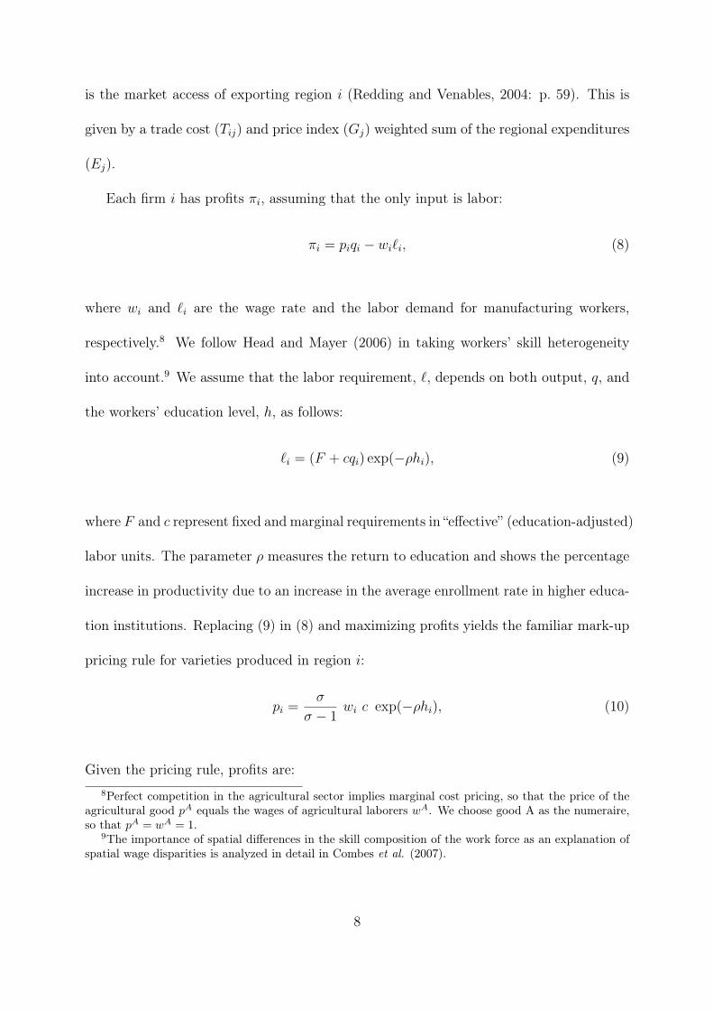
into account.9 We assume that the labor requirement, `, depends on both output, q, and

the workers’ education level, h, as follows:

`i = (F + cqi) exp(−ρhi), (9)

where F and c represent fixed and marginal requirements in “effective” (education-adjusted)

labor units. The parameter ρ measures the return to education and shows the percentage

increase in productivity due to an increase in the average enrollment rate in higher educa-

tion institutions. Replacing (9) in (8) and maximizing profits yields the familiar mark-up

pricing rule for varieties produced in region i:

pi =σ

σ − 1wi c exp(−ρhi), (10)

Given the pricing rule, profits are:8Perfect competition in the agricultural sector implies marginal cost pricing, so that the price of the

agricultural good pA equals the wages of agricultural laborers wA. We choose good A as the numeraire,so that pA = wA = 1.

9The importance of spatial differences in the skill composition of the work force as an explanation ofspatial wage disparities is analyzed in detail in Combes et al. (2007).

8

πi = wi

[cqi

(exp(−ρhi)

σ − 1

)− F exp(−ρhi)

]. (11)

We assume that free entry and exit drive profits to zero. This condition implies that

the equilibrium output of any firm is:

q∗ =F (σ − 1)

c. (12)

Using the demand function (6), the pricing rule (10) and equilibrium output (12), we

calculate the manufacturing wage when firms break even:

wi =σ − 1

σc exp(−ρhi)

[µMAi

c

F (σ − 1)

]1/σ

. (13)

2.3 Deviation from the short-run equilibrium

Despite the lack of any explicit dynamics in the model, it is useful to consider wage

equation (13) as a short-run equilibrium, taking as given the allocation of workers in

each region.10 This equilibrium is consistent with the existence of short-run frictions in

labor mobility across Chinese provinces. Even if the volume of internal migration has been

increasing in China due to more relaxed migration policies, the hukou system of household

registration still restricts labor mobility across regions (Au and Henderson, 2006).11 The

associated equilibrium labor demand for workers in province i is given by:

`∗i = σF exp(−ρhi). (14)

We now aim to work out the direct effects of an immigrant labor supply shock on10This assumption defines a Marshallian short-run equilibrium (see Krugman, 1991).11Amiti and Javorcik (2007) raise a similar point investigating the location of foreign firms in China.

9

wages, i.e. a reallocation of workers across provinces. To this end, we turn equation (14)

around and express fixed requirements as:

F =`∗i

σ exp(−ρhi). (15)

Replacing (15) in the wage equation (13) gives:

wi = (σ − 1)σ−1

σ (µMAi)1σ [cσ exp(−ρhi)]

1−σσ `∗

− 1σ

i . (16)

We take logs and rearrange equation (16):

ln wi = α0 + α1 ln MAi + α2hi + α3 ln `∗i + εi, (17)

where α0 = σ−1σ

ln(σ− 1)+ 1σ

ln µ+ 1σ

ln cσ, α1 = 1σ, α2 = σ−1

σρ, and α3 = − 1

σ. Estimating

this equation, we expect, first, that the elasticity of substitution (σ) between traded goods

will be greater than one and, second, that the elasticities of market access and labor supply

will be equal in absolute value.

In order to depart from the preimmigration market equilibrium situation `∗i and inves-

tigate the direct effect of a reallocation of workers across provinces we draw on the labor

economics literature. More precisely, we follow the methodology of Friedberg (2001) and

Borjas (2003) regarding the effect of immigration on wages. They assume an exogenous

influx of immigrant labor supply mi in region i. The resulting rate of change of labor

supply due to immigration is given by mi/`i ≈ ln(`i + mi) − ln(`i). Using this, we can

work out the direct effect of an exogenous inflow of immigrants by estimating the following

equation:ln wi = α0 + α1 ln MAi + α2hi + α3

mi

`i

+ εi. (18)

10

Equation (18) is a reduced-form wage specification relating the regional manufactur-

ing wage to market access, educational attainment, an exogenous rate of change of labor

supply due to immigration and the usual error term εi. The assumption of an exogenous

influx of immigrant labor supply mi is a convenient assumption. It avoids an explicit mod-

eling of a labor supply function for migration. The migration decision is however expected

to be driven by an income differential between the origin and destination provinces. Con-

sequently, the exogeneity of our labor supply shock may be a concern. To deal with this

problem we estimate equation (18) with an instrumental variable approach, as discussed

below.

3 Data and estimation issues

Using equation (18), the core empirical part of this paper explains the variation in average

provincial manufacturing wages in China. Before proceeding to the estimations, we first

describe the data.

3.1 Data

We explain here how the dependent and independent variables are constructed. Appendix

B.1 provides greater details regarding the data sources. Table 3 in Appendix C provides

summary statistics for all of the variables.

11

3.1.1 Dependent variable

The dataset covers 29 Chinese provinces over the period 1997-2004.12 Our dependent

variable is the average annual nominal wage rate of manufacturing workers and staff.

This is defined as the ratio of the total wage bill to the number of manufacturing workers

and staff by province and year.

3.1.2 Explanatory variables

We detail here the construction of market access and immigrant labor supply (Appendix

B.1 provides details about the other explanatory variables).

Construction of market access

Recall from equation (7) that the market access variable is defined as a trade cost and

price index weighted sum of the regional expenditures. In order to compute a measure for

the market access of province i, we follow a strategy, pioneered by Redding and Venables

(2004), that exploits information from the estimation of bilateral trade. However, Redding

and Venables (2004) simply assume that trade costs depend on bilateral distance. We

instead allow for differentiated trade cost measures depending on whether trade occurs

within province/country, between provinces or between countries.

Summing (Eq. 5) over all of the products produced in location i, we obtain the total

value of the exports of i to j:

Xij = µni(piTij)1−σ Gσ−1

j Ej = µsci φij mcj, (19)

12The entire country is divided into 27 provinces plus four province-status “super-cities” – Beijing,Chongqing, Shanghai and Tianjin. Our analysis covers all of the provinces apart from Tibet. Chongqingand Sichuan are considered together.

12

where ni is the set of varieties produced in region i, sci = ni(pi)1−σ measures the “supply

capacity” of the exporting region, mcj = Gσ−1j Ej the “market capacity” of region j, and

φij = T 1−σij the “freeness” of trade (Baldwin et al., 2003).13 Freeness of trade is assumed to

depend on bilateral distances (distij) and a series of dummy variables indicating whether

provincial or foreign borders are crossed.

φij = dist−δij exp

[−ϕBf

ij − ϕ∗ Bf∗ij + ψContigij − ϑ Bc

ij + ξ Biij + ζij

], (20)

where Bfij = 1 if i and j are in two different countries with either i or j being China

and 0 otherwise, Bf∗ij = 1 if i and j are in two different countries with neither i nor j being

China and 0 otherwise, Contigij = 1 if the two different countries i and j are contiguous,

and 0 otherwise, Bcij = 1 if i and j are two different Chinese provinces and 0 otherwise, and

Biij = 1 if i = j denotes the same foreign country and 0 otherwise. The error ζij captures

the unmeasured determinants of trade freeness. Consequently, this specification allows

the impediments to domestic trade to be different from the impediments to international

trade (see Appendix D for details).

Substituting (20) into (19), capturing unobserved exporting (ln sci) and importing

(ln mcj) region characteristics à la Redding and Venables (2004) with exporting and im-

porting fixed effects (ctyi and ptnj) and taking logs yields the following trade regression:

ln Xij = ln µ+ctyi+ptnj−δ ln distij−ϕBfij−ϕ∗ Bf∗

ij +ψContigij−ϑ Bcij +ξ Bi

ij +ζij. (21)

Using our complete dataset of trade (see Appendix B.2 for details), we estimate equa-

tion (21) on a yearly basis from 1995 to 2002. The estimation of the gravity equation13φij ∈ [0, 1] equals 1 when trade is free and 0 when trade is eliminated due to high shipping costs and

elasticity of substitution (σ).

13

in cross-section, for each year of the sample, with region fixed effects is recommended by

trade theory. The yearly estimated coefficients of equation (21) are then used to construct

predicted values for market access defined as MAi =∑R

j=1 φijmcj.14 Our estimated mar-

ket access variable consists of three parts: local market access (intra-provincial demand);

national market access (demand from other Chinese provinces); and world market access:

M̂Ai = φ̂iiGσ−1i Ei +

∑

j∈P

φ̂ijGσ−1j Ej +

∑

j∈F

φ̂ijGσ−1j Ej (22)

= exp(ptni)× dist−δ̂ii +

∑

j∈P

exp(ptnj)× dist−δ̂ij × exp(ϑ)

+∑

j∈F

exp(ptnj)λ̂ × dist−δ̂

ij × exp(ϕ̂ + ψ̂Contigij),

where P and F stand for Chinese provinces and foreign countries, respectively. The

results for various years are presented in Table 3 of Appendix D.

Map 1 shows that coastal provinces had greater market access and higher nominal

wages in manufacturing in 2002. One exception is Shandong province, with high market

access and below median wages.

Immigrant share

The rate of change of labor supply resulting from immigration is given by the inter-

nal migration share (mi

`i). We rely on the annual Sample Survey on Population Changes

to compute this share as the number of non-residents divided by the population.15 We

actually assume that the number of non-residents in a province is a good proxy for im-14Equation (21) also allows us to construct empirical predictions for supplier access, SAj , defined

as SAj =∑

i φijsci. However, since market access and supplier access variables tend to be highlycorrelated (see Amiti and Javorcik, 2007, in the Chinese context), we follow most of the NEG literatureand concentrate on market access forces.

15The results remain unchanged if we use the number of permanent residents in a province as a proxyfor `i; these are available upon request. Permanent residents are defined as the population “residing intownship, towns and street communities with permanent household registration there”, i.e. in province i.

14

Map 1: Nominal manufacturing wages and constructed market access in China (2002)

Bubles correspond to the magnitude of provincial market access

Yearly manufacturing wage (yuans)

migrant labor supply (mi). Non-residents in a province are defined as the population

living in “township, towns and street communities with permanent household registration

elsewhere, [and] having been away from that place for less than one year”.

3.2 Estimation issues

A first estimation issue refers to the use of average annual earnings per worker to mea-

sure wages. In fact, “cross-region variation in worker characteristics may reflect regional

characteristics that are constant over the sample period” (Hanson, 2005). However, as in

Hanson (1996), we are not able to control directly for fixed provincial effects by including

dummy variables for provinces, as this would introduce perfect multicollinearity into the

regressions. First-differencing is another way to eliminate province effects from the regres-

sion but it is not without problems either, as it may exacerbate potential problems with

15

noise (Altonji, 1986) or measurement errors in the data (Griliches and Hausman, 1986).

We thus estimate Eq. (18) in levels with additional controls. These latter help to mitigate

omitted variable bias. We thus account for the province-status of “super-cities” (munici-

pality),16 the number of Special Economic Zones (SEZ ),17 the features of the coastal and

Western provinces compared to interior regions18 and a set of year-specific intercepts.19

This specification fits the data well and explains a large part of the variance in provincial

wages.

A second estimation issue relates to the endogeneity of the immigration shock. As men-

tioned above, we use an instrumental variable approach. The reliability of this method

lies on the identification of instruments which are correlated with the inflow of immigrants

but uncorrelated with the error term, i.e. with the unobserved component of wages. One

first exogenous source of variation in migrant flows may be found in climate variables (see

Roback, 1982). We argue that unfavorable climate conditions in the province of origin

may augment potential migrants’ probability of departure. We consider two complemen-

tary climate dimensions: annual temperature and annual precipitation in major cities.

Using the 1990 Census (National Bureau of Statistics of China, 1991), we compute an

annual weighted average of climate conditions in the province of origin j for each of these

dimensions. The weight is the share of province of origin j in the total immigration re-16The three province-status cities (Beijing, Shanghai and Tianjin) may exhibit specific features such as

smaller surface areas, more developed transport infrastructure, and greater proximity to administrativepower. Municipalityi is a binary variable which equals one if i is one of the three province-status cities.

17Three SEZ were opened in 1980 in Guangdong province and one in Fujian province in 1981. Theseopen areas adopted preferential policies and played the role of windows in developing the foreign-orientedeconomy, generating foreign exchange via exports and importing advanced technology. SEZi is computedas the number of Special Economic Zones in the province (and equals 0, 1, 2 or 3).

18Coastali is a binary variable which equals one if i is a coastal province, and Westi is a binary variablewhich equals one if i is a Western province.

19We also introduced the distance to Hong Kong as an additional regressor to check if market access isrelated to the export-processing trade with Hong Kong. The estimated coefficient on this variable turnedto be statistically insignificant in all of the regressions. These results are available upon request.

16

ceived by province i (termed “immigrationij”) between 1985 and 1990.20 More precisely,

each instrument relating to destination province i is calculated as:

Imigclimateti=

∑

j 6=i

climatetj

immigrationij∑j 6=i immigrationij

,

with climate referring either to temperature (Imigtempti) or rainfall (Imigt

raini) data. To

ensure the exogeneity of these indicators, we exclude information from province i in their

calculation. We also introduce the annual averages of temperature and precipitation of the

major cities in province i as additional control variables in the wage equation: this ensures

that the instruments are not simply proxying the climate conditions in the destination

province. Since we do not have any a priori ideas about the appropriate specification

of the relationship between climate and immigrant share in the destination population,

we allow for a quadratic relationship in the instrumental equation. A second source of

exogeneity refers to geography. The surface area of the destination province, measured in

square kilometers, may influence the extent of immigration; this is employed as our third

instrument.

A third estimation issue relates to the market access variable, which appears on the

right-hand side of the estimated equation (18). This represents a weighted sum of regional

expenditures. However, these expenditures themselves depend on income, and therefore

on wages, raising the issue of reverse causality. A positive shock to wi will increase Ei

and thus MAi (Head and Mayer, 2006).21 To deal with this problem, we first follow

Redding and Venables (2004) and lag the market access variable by two years to avoid20Such bilateral measures of immigration are build from census data and only available every five years.21This will be all the more problematic since φij < φii. In the case of extremely high inter-provincial

and international transport costs (φij = 0, ∀ i 6= j), only local expenditure enters MAi.

17

contemporaneous shocks that affect both the left- and right-hand side variables. We

then appeal to an instrumental variable strategy. The literature so far has attempted

to resolve this simultaneity problem by picking out variations in market access which

result from geographic variables. While Redding and Venables (2004) use the distance to

the nearest central place (Brussels, New York City, or Tokyo), Head and Mayer (2006)

use measures of “centrality” of locations obtained by dividing the surface of the globe into

approximately 11,700 squares. Both measures can reasonably be assumed to be exogenous

to potential wage shocks since they do not include any information on regional market

size. However, they do have the disadvantage of being time invariant, and as such only

explain the cross-section dimension of market access. Our aim is to account for both

the within and cross-sectional dimensions in our sample. We therefore follow a different

approach and rely on an instrument for demand in location i at time t which is based

on the weighted average of the yearly variations in the nominal exchange rate (NER)

of importing partners. This instrument for the market access of Chinese province i is

calculated as:

Imati=

∑

j

∆NERtij1

distij,

with ∆NER being the first difference in the nominal exchange rate between partner j’s

currency and the Chinese Yuan. The variation in NERij is weighted by the distance

of country i to j (distij)22. Since bilateral exchange rates are similar across Chinese

provinces, the instrumentation strategy relies entirely on the heterogeneity of import

partners across Chinese provinces. We thus argue that a nominal devaluation (apprecia-

tion) of country j’s currency vis-à-vis the Chinese Yuan translates into a fall (rise) in j’s22Our results are robust to the use of a different weight, defined as the share of country j in the exports

of province i to j in 1995.

18

demand (market capacity) for products from China. The impact of that change differs

across Chinese provinces depending on an exogenous factor: the distance to partner j.

4 Estimation results

We now proceed to the estimation of the wage equation derived in section 2.3. We run

Eq. (18) for 29 provinces over the period 1997-2004. Table 1 reports the results of this

baseline specification. Our NEG wage equation fits quite well the data by explaining

approximately 80 to 90% of the variation in average provincial wages.

Column (1) reports the results from the OLS estimation of Eq. (18) without the

immigrant share but with additional controls and a two-year lagged measure of market

access (as discussed in section 3 above we later instrument for the market access).23 It is

useful to interpret the size of the estimated coefficients. Holding other factors constant, a

10% increase in market access raises wages by about 1% on average. In addition, a one-

point increase in students enrolled in institutions of higher education as a percentage of the

population raises wages roughly by 28%. All of the additional controls enter positively and

significantly, highlighting the wage premium accruing to the three province-status “super-

cities”, the two provinces hosting SEZs and the coastal and Western provinces compared

to interior regions.24 The estimated coefficients on the Year dummies are significant

and increase over time, showing the influence of common upward pressure on wages (see

below).23Since the predicted values of market access are generated from a previous trade regression, we check

the sensitivity of our results using bootstrap techniques: the results remained unchanged. The boot-strapped standard errors (500 replications) are available upon request.

24The wage differential between Western and interior provinces may be explained by the employmentopportunities in industries offering high wages and salaries in Western China, such as oil and gas compa-nies, as well as border trade companies with Central Asian countries. Note, however, that this differenceis not robust to the instrumental variable estimates in Cols. 2-6.

19

Table 1: Manufacturing wage equationDependent Variable: ln(Manufacturing wage)

Column: (1) (2) (3) (4) (5) (6)Method: OLS IV IV IV IV IVLagged ln(Market Access)a 0.10 0.16 0.16 0.15 0.16 0.25

(0.01)∗∗∗

(0.03)∗∗∗

(0.03)∗∗∗

(0.02)∗∗∗

(0.03)∗∗∗

(0.07)∗∗∗

Higher-Education Ratio 0.28 1.12 0.72 0.66 0.77 0.83(0.10)

∗∗∗(0.40)

∗∗∗(0.27)

∗∗∗(0.25)

∗∗∗(0.29)

∗∗∗(0.31)

∗∗

Immigrant Share -0.04 -0.03 -0.03 -0.03 -0.04(0.01)

∗∗∗(0.01)

∗∗∗(0.01)

∗∗∗(0.01)

∗∗∗(0.01)

∗∗∗

Population -0.00 -0.00 -0.00 -0.00(0.00)

∗∗∗(0.00)

∗∗∗(0.00)

∗∗∗(0.00)

∗∗

Municipality-dummy 0.30 0.48 0.38 0.38 0.37 0.20(0.05)

∗∗∗(0.09)

∗∗∗(0.07)

∗∗∗(0.07)

∗∗∗(0.07)

∗∗∗(0.15)

Special Economic Zones 0.06 0.10 0.08 0.08 0.08 0.04(0.02)

∗∗∗(0.03)

∗∗∗(0.02)

∗∗∗(0.02)

∗∗∗(0.02)

∗∗∗(0.04)

Coast dummy 0.06 0.02 0.01 0.02 -0.01 -0.07(0.02)

∗∗∗(0.04) (0.03) (0.03) (0.04) (0.07)

West dummy 0.12 0.04 0.05 0.06 0.05 0.01(0.02)

∗∗∗(0.05) (0.04) (0.04) (0.04) (0.06)

Rain 0.01 0.01 0.01 0.01 0.01(0.00)

∗∗∗(0.00)

∗∗∗(0.00)

∗∗∗(0.00)

∗∗∗(0.00)

∗∗∗

Temperature -0.32 -0.06 0.01 0.11 0.55(0.31) (0.27) (0.26) (0.29) (0.45)

Year 1998 b 0.17∗∗∗

0.17∗∗∗

0.17∗∗∗

0.17∗∗∗

0.17∗∗∗

0.18∗∗∗

Year 1999 0.28∗∗∗

0.29∗∗∗

0.29∗∗∗

0.29∗∗∗

0.29∗∗∗

0.31∗∗∗

Year 2000 0.41∗∗∗

0.70∗∗∗

0.63∗∗∗

0.61∗∗∗

0.64∗∗∗

0.73∗∗∗

Year 2001 0.49∗∗∗

0.67∗∗∗

0.63∗∗∗

0.62∗∗∗

0.64∗∗∗

0.69∗∗∗

Year 2002 0.59∗∗∗

0.69∗∗∗

0.67∗∗∗

0.66∗∗∗

0.67∗∗∗

0.71∗∗∗

Year 2003 0.72∗∗∗

0.81∗∗∗

0.80∗∗∗

0.80∗∗∗

0.80∗∗∗

0.84∗∗∗

Year 2004 0.84∗∗∗

0.94∗∗∗

0.93∗∗∗

0.93∗∗∗

0.93∗∗∗

0.97∗∗∗

No. of Observations 232 232 232 232 232 232Adj. R-squared 0.92 0.80 0.87 0.87 0.86 0.79Durbin-Wu-Hausman test 17.01 18.07 18.00 18.05 29.90[p− value] [0.00]

∗∗∗[0.00]

∗∗∗[0.00]

∗∗∗[0.00]

∗∗∗[0.00]

∗∗∗

Hansen J-Statistic 5.94 3.74 4.25 3.51 0.59[p− value] [0.20] [0.44] [0.37] [0.47] [0.96]Stock-Wright S-Statistic 22.27 24.14 24.14 24.14 23.99[p− value] [0.00]

∗∗∗[0.00]

∗∗∗[0.00]

∗∗∗[0.00]

∗∗∗[0.00]

∗∗∗

Shea Partial R2 (1st-stage) (in %)Immigrant Share 3.31 6.16 6.79 5.67 6.38Population 73.29 70.50 76.30 46.72Lagged ln(Market Access) 8.42

Notes: Heteroscedastic-consistent standard errors in parentheses, with ∗∗∗, ∗∗ and ∗ denoting signifi-cance at the 1, 5% and 10% levels, respectively. aMarket access is two-year lagged to abstract fromcontemporaneous shocks that affect both left- and right-hand side variables. bTo save space, we donot report the constant and the standard errors of the year dummies. Standard errors vary between0.03 and 0.09 and are available upon request. Col. (1) estimates Eq. (18) without the immigrant sharebut with additional controls. Columns (2) to (6) include the immigrant share, defined as non-residentsover population in cols. (2), (3) and (6), as female non-residents over population in col. (4), and asmale non-residents over population in col. (5). Instrumented variables (depending on the specifica-tion): Immigrant Share, Population, two-years lagged ln(Market Access). Instruments (depending onthe specification): area, climate variables (Imigtemp and Imigrain) and their square, two-year laggedpopulation and two-year lagged Ima. See the text for more details.

20

In columns (2) to (6), we include immigrant share. These estimations are based on

instrumental variables (IV), which allows us to control for any simultaneity between wages

and immigration. As described above, we appeal to three different instruments.

The small p-value of the Durbin-Wu-Hausman test, in all of the IV estimations, con-

firms that the OLS estimator is not consistent and that IV techniques are preferred. As a

precondition for the reliability of the procedure, we check the validity of our instruments

via the Hansen test of overidentifying restrictions. The resulting insignificant test statistic

indicates that the orthogonality of the instruments to the error term cannot be rejected,

so that our instruments are appropriate. Both test statistics are reported at the bottom of

the results in Table 1. The Shea partial R2 is a measure of instrument relevance and takes

into account the collinearity between the endogenous variables (Shea, 1997). The Shea

R2 is fairly low in specification (2), but this was expected since the endogenous migration

variable is already well explained by the instruments included, i.e. the exogenous vari-

ables of the second stage regression.25 Moreover, we include the Stock and Wright (2000)

statistic that provides weak-instrument robust inference for testing the significance of the

endogenous regressors. We reject the null hypothesis that the coefficients of the excluded

instruments are jointly equal to zero.

Before elaborating on the negative impact of the immigrant share estimate, we check

the sensitivity of our results in columns (3) to (6). In column (3), we follow Borjas (2003)

and address the interpretation problem that a rise in the immigrant share can represent

either an increase in the number of non-residents or a fall in population. We thus add

the province’s population level as a regressor and the two-year lagged value of population25This might raise concerns about multicollinearity, but the auxiliary R2 of the first stage regression,

with or without the excluded instruments, is lower than the overall R2 of the second stage.

21

as an additional instrument. Controlling for this size variable does not much change the

results.

Current international migration is different from past mass migration, when immi-

grants were disproportionately men (Freeman, 2006). As in current international migra-

tion, nearly half of the current immigrants in China are women (see Table 3 in Appendix

C). Our results still hold if we take this new trend into account and redefine the immigrant

share as female non-residents over population in column (4), and as male non-residents

over population in column (5).

In the last column of Table 1, we address the simultaneity problem of market access

and wages via instrumental variables, as detailed above. The high p-value of the Hansen

test of overidentifying restrictions indicates that our instrumentation is appropriate. It is

worth noting that the estimate on market access is now much higher (column 6).

The estimates confirm the positive influence of market access and education on wages.

The structural derivation of our market access variable from theory provides us with a

theoretical interpretation of its coefficient: this figure corresponds to 1/σ, with σ being a

measure of product differentiation. Our estimates of the elasticity of substitution between

traded goods are greater than unity and range between 4 and 6.7, depending on the

IV specification used. This is consistent with theory and roughly in line with recent

estimates in the NEG (Hanson, 2005) and international trade literatures (Head and Ries,

2001). Hanson’s (2005) estimates of σ range in value between 4.9 and 7.6. Our results

also underline that an increase in the immigrant share, defined as non-residents over

population, imposes downward pressure on the destination region’s wage. The effect is

22

statistically and economically highly significant. On average, a one-point increase in the

immigrant share induces a fall in average wages by approximately 4% (col. 6). As a

consequence, in the context of high immigration flows, a manufacturing firm, given its

access to markets and other regional characteristics, can afford to pay lower wages.

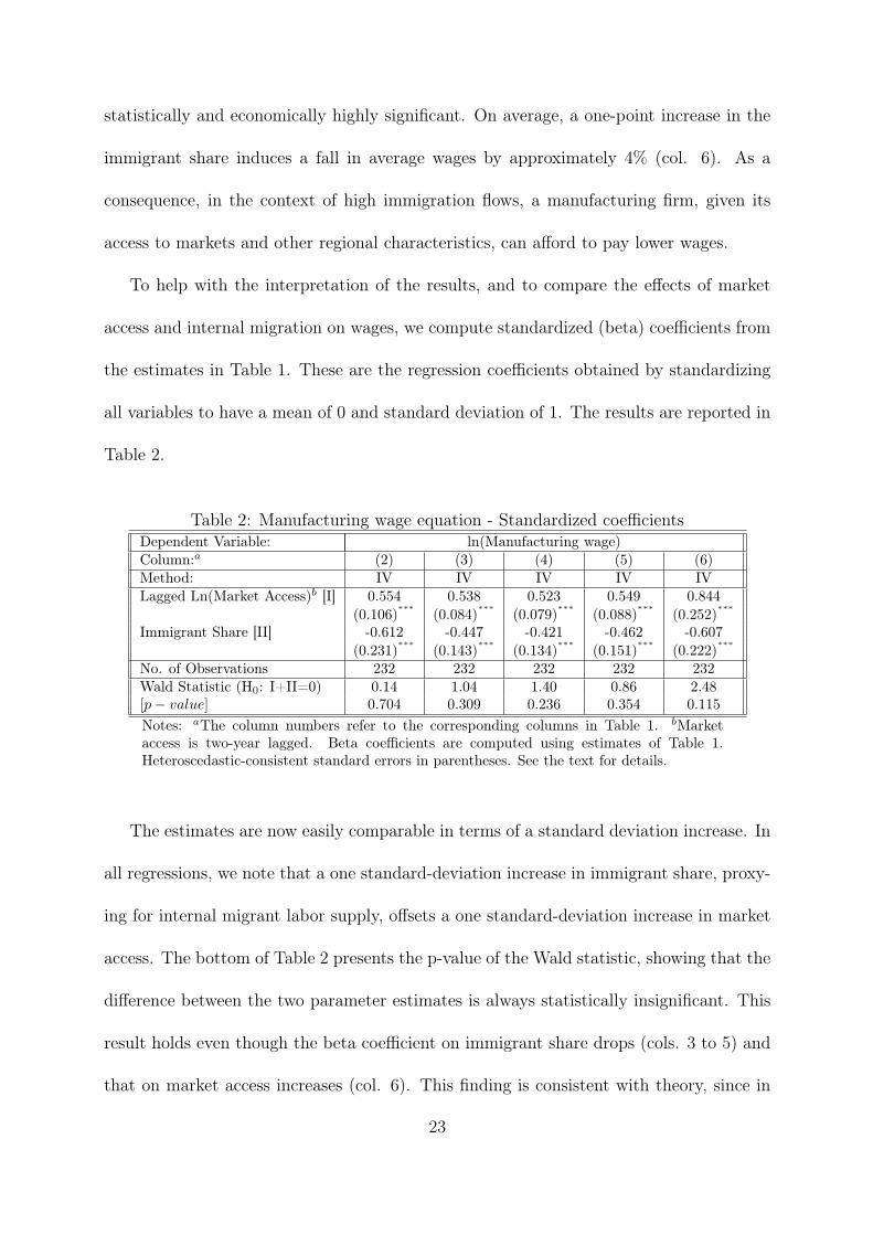
To help with the interpretation of the results, and to compare the effects of market

access and internal migration on wages, we compute standardized (beta) coefficients from

the estimates in Table 1. These are the regression coefficients obtained by standardizing

all variables to have a mean of 0 and standard deviation of 1. The results are reported in

Table 2.

Table 2: Manufacturing wage equation - Standardized coefficientsDependent Variable: ln(Manufacturing wage)Column:a (2) (3) (4) (5) (6)Method: IV IV IV IV IVLagged Ln(Market Access)b [I] 0.554 0.538 0.523 0.549 0.844

(0.106)∗∗∗

(0.084)∗∗∗

(0.079)∗∗∗

(0.088)∗∗∗

(0.252)∗∗∗

Immigrant Share [II] -0.612 -0.447 -0.421 -0.462 -0.607(0.231)

∗∗∗(0.143)

∗∗∗(0.134)

∗∗∗(0.151)

∗∗∗(0.222)

∗∗∗

No. of Observations 232 232 232 232 232Wald Statistic (H0: I+II=0) 0.14 1.04 1.40 0.86 2.48[p− value] 0.704 0.309 0.236 0.354 0.115Notes: aThe column numbers refer to the corresponding columns in Table 1. bMarketaccess is two-year lagged. Beta coefficients are computed using estimates of Table 1.Heteroscedastic-consistent standard errors in parentheses. See the text for details.

The estimates are now easily comparable in terms of a standard deviation increase. In

all regressions, we note that a one standard-deviation increase in immigrant share, proxy-

ing for internal migrant labor supply, offsets a one standard-deviation increase in market

access. The bottom of Table 2 presents the p-value of the Wald statistic, showing that the

difference between the two parameter estimates is always statistically insignificant. This

result holds even though the beta coefficient on immigrant share drops (cols. 3 to 5) and

that on market access increases (col. 6). This finding is consistent with theory, since in

23

absolute value the estimate on labor supply is roughly equal to the estimate on market

access.

The results in column (6), controlling for the endogeneity of migration and market

access, are our preferred estimates. They suggest that both migration and market access

are statistically and economically highly significant. Another interesting result emerges.

Based on the estimated year dummies, we find, holding other factors constant, that provin-

cial wages increased on average by about 15% per year between 1997 and 2004.26 This

trend is common to all provinces and may be explained by common shocks like total fac-

tor productivity growth27, the national rise in service-sector prices28 and social security

reforms increasing minimum wages.

5 Conclusion and discussion

This paper has examined the importance of economic geography and migration in explain-

ing the spatial structure of wages in China. Our econometric specification relates wages

to a transport-cost weighted sum of demand in surrounding locations and to migratory

inflows. We estimate the maximum wage a firm can afford to pay, given market access

and immigrant labor supply. The data come from a sample of 29 Chinese provinces be-

tween 1997 and 2004. We moreover control for various endogeneity issues via instrumental

variables.

Overall our results highlight that rapidly increasing wages in China correspond to a26To calculate this average, we first-difference the year dummy estimates and then compute the geo-

metric mean of the antilog-transformed differences.27Recent estimates suggest that China’s total factor productivity grew at an annual rate of 4% over

the period 1993-2004 (Bosworth and Collins, 2006).28Recall from Eq. (7) that we control for the manufacturing price index.

24

common national trend. Since total factor productivity growth appears to explain only

one third of this trend, the China price has increased over the period. In the meantime,

we find that migration flows have slowed down Chinese wage increase. On average the

immigrant share has increased from 5 to 9% between 1997 and 2004. Given a one-point

increase in the immigrant share, average wages fall by approximately 4%; this more intense

internal migration has thus slowed down wage growth by 16% in total (2.5% per year). It

is however possible that the further relaxation of migration restrictions, claimed by the

export-intensive provinces, will lead to a different scenario. In the extreme case where the

average migrant share triples to reach 30% (the value for Beijing in 2004), the downward

pressure on wages could be as great as 80%. In that case, the China price will remain

unbeatable.

Average provincial access to national and international markets has shown less move-

ment. It has grown, but at a much lower rate (a little less than 20%) on average, producing

a wage rise of 5%, given a market elasticity of 0.25. The wage impact of market access is

thus three times smaller in magnitude than the effect of migration (and of the opposite

sign). Market access appears so far to have played a limited role. However, this not a

much surprising finding since agglomeration effects take time to materalize.

ReferencesAdams, F.G., Gangnes G. and Y. Shachmurove, 2006, “Why is China so Competitive?

Measuring and Explaining China’s Competitiveness,” World Economy, 29(2), 95-122.

Altonji, J., 1986, “Intertemporal substitution in labor supply: Evidence from micro data,”Journal of Political Economy, 94(3.2), 176-215.

Amiti, M. and B.S. Javorcik, 2007, “Trade Costs and Location of Foreign Firms in China,”Journal of Development Economics, forthcoming.

25

Au, C.-C. and V. Henderson, 2006, “How Migration Restrictions Limit Agglomerationand Productivity in China,” Journal of Development Economics, 80(2), pp. 350-388.

Borjas, G.J., 2003, “The Labor Demand Curve Is Downward Sloping: Reexamining theImpact of Immigration on the Labor Market,” Quarterly Journal of Economics,118(4), 1335-74.

Bosworth, B. and S. Collins, 2006, “Accounting for growth: Comparing China and India,”mimeo.

Breinlich H., 2007, “The Spatial Income Structure in the European Union - What Rolefor Economic Geography?,” Journal of Economic Geography, forthcoming.

Card, D., 2001, “Immigrant Inflows, Native Outflows and the Local Labor Market Im-pacts of Higher Immigration,” Journal of Labor Economics, 19, 2261.

Combes, P.-P., G. Duranton and L. Gobillon, 2007, “Spatial Wage Disparities: SortingMatters!,” Journal of Urban Economics, forthcoming.

Freeman, R., 2006, “People flows in globalization,” Journal of Economic Perspectives,20(2), 145-170.

Friedberg, R., 2001, “The Impact of Mass Migration on the Israeli Labor Market,” Quar-terly Journal of Economics, 116(4), 1373-1408.

Fujita, M., P. Krugman and A.J. Venables, 1999, The Spatial Economy: Cities, Regionsand International Trade, MIT Press, Cambridge.

Griliches, Z., and J. Hausman, 1986, “Errors in Variables in Panel Data,” Journal ofEconometrics, 31, 93-118.

Hanson, G., 1996, “Localization Economies, Vertical Organization, and Trade,” AmericanEconomic Review, 86, 1266-1278.

Hanson, G., 2005, “Market Potential, Increasing Returns, and Geographic Concentra-tion,” Journal of International Economics, 67(1), 1-24.

Harris, C., 1954, “The Market as a Factor in the Localization of Industry in the UnitedStates”, Annals of the Association of American Geographers, 64, 315-48.

Head, K., and J. Ries, 2001, “Increasing Returns Versus National Product Differentia-tion as an Explanation for the Pattern of U.S.-Canada Trade,” American EconomicReview, 91(4), 858-75.

Head, K., and T. Mayer, 2006, “Regional Wage and Employment Responses to MarketPotential in the EU,” Regional Science and Urban Economics, 36(5), 573-594.

Krugman, P., 1991, “Increasing Returns and Economic Geography,” Journal of PoliticalEconomy, 99(3), 483-499.

Lett, E and J. Banister, 2006, “Labor Costs of Manufacturing Employees in China: anUpdate to 200304,” Monthly Labor Review, November.

26

Lin, S., 2005, “Geographic Location, Trade and Income Inequality in China,” in SpatialInequality and Development, Kanbur R. and A.J. Venables (eds.), Oxford UniversityPress, London.

National Bureau of Statistics of China, China Statistical Yearbooks, People’s Republicof China. Beijing, China Statistical Press, various years.

National Bureau of Statistics of China, China Labor Statistical Yearbook, People’s Re-public of China. Beijing, China Statistics Press, various years.

National Bureau of Statistics of China, Cities China 1949-1998, Xin Zhongguo Chengshi50 Nian, People’s Republic of China, Beijing: Xinhua Press, 1999.

National Bureau of Statistics of China, 1991, 10 percent Sampling Tabulation on the1990 Population Census of the People’s Republic of China. Beijing, China StatisticalPublishing House.

National Bureau of Statistics of China, 1997, Figure of 1% Population Sample Survey in1995. Beijing, China Statistical Publishing House.

National Bureau of Statistics of China, 2002, Figures on 2000 Population Census ofChina (CD-ROM), Beijing, China Statistics Press.

Ottaviano, G.I.P. and D. Pinelli, 2006, “Market Potential and Productivity: Evidencefrom Finnish Regions,” Regional Science and Urban Economics, 36, 636657.

Redding, S. and A.J. Venables, 2004, “Economic Geography and International Inequal-ity,” Journal of International Economics, 62(1), 53-82.

Roback, J., 1982, “Wages, Rents, and the Quality of Life,” Journal of Political Economy,90(6), 1257-78.

Shea, J., 1997, “Instrument Relevance in Multivariate Linear Models: a Simple Measure,”Review of Economics and Statistics, 79(2), 348-52.

Shen, J., 1999, “Modeling Regional Migration in China: Estimation and Decomposition,”Environment and Planning, 31(7), 1223-1238.

Stock, J.H. and J.H. Wright, 2000, “GMM with Weak Identification,” Econometrica,68(5), 1055-96.

Wei, S-J., 1996, “Intra-national versus International Trade: How Stubborn are Nationsin Global Integration?,” NBER Working Paper 5531.

27

Appendix A: Wage growth

Figure 1: Manufacturing wage growth (1996-2004)3

.23

.43.6

3.8

44

.2L

og

of

ave

rag

e

rea

l m

an

ufa

ctu

rin

g

wa

ges

1996 1998 2000 2002 2004Year

Appendix B: Data descriptions and sources

This appendix describes the data sources and explains the construction of the indicatorsused in the estimations.

B.1. Province-level data

The wage equation relies on various indicators constructed using the China StatisticalYearbooks which provide data on average nominal wages for formal employees, population,climate and migration. All of these economic indicators are provided at the provinciallevel, including province-status municipalities.

The education variable is calculated as the ratio of the number of students enrolled ininstitutions of higher education to the population. Institutions of higher education referto establishments which have been set up according to government evaluation and ap-proval procedures, enrolling high-school graduates and providing higher-education coursesand training for senior professionals. They include full-time universities, colleges, andhigher/further education institutes.

28

B.2. Trade data

Various data sources have been used to estimate the trade equation on both internationaland intra-national trade flows for China and its foreign partners.

B.2.1. International Data

International trade flows are expressed in current USD and come from IMF Direction ofTrade Statistics (DOTS).

Internal trade flows are expressed in current USD and are calculated as the differencebetween domestic primary and secondary sector production minus exports.

Production data for OECD countries come from the OECD STAN database. Forother countries, the ratios of industry and agriculture output as a percentage of GDP areextracted from Datastream. These are then multiplied by country GDP (in current USD)from World Development Indicators 2005.

B.2.2. Chinese Data

The provincial foreign trade data are obtained from the Customs General Administrationdatabase, which records the value of all import and export transactions which pass viaCustoms. Provincial imports and exports are decomposed into those concerning up to230 international partners. This database has previously been discussed by Lin (2005)and Feenstra, Hai, Woo and Yao (1998).

The exchange rate is the average exchange rate of the Yuan against the US dollar inthe China Exchange Market. This comes from the China Statistical Yearbook.

Production data for Chinese provinces are calculated as the sum of industrial andagricultural output. Output in Yuan are converted into current USD using the annualexchange rate. All statistics come from China Statistical Yearbooks.

Provincial input-output tables29 provide the decomposition of provincial output, andthe international and domestic trade of tradable goods. These are available for 28provinces, with data missing for Tibet, Hainan and Chongqing.

29Most Chinese provinces produced square input-output tables for 1997. A few of these are publishedin provincial statistical yearbooks. We obtained access to the final-demand columns of these matricesfrom the input-output division of China’s National Bureau of Statistics. Our estimations assume that theshare of domestic trade flows (that is between each province and the rest of China) in the total provincialtrade is constant over time.

29

Appendix C: Summary statistics

Table 3: Summary Statistics, 1995-2004Obs Mean St. Dev. Minimum Maximum

Dependent Variable:Manufacturing Wage 232 9,431 3,714 3,903 27,456ln(Manufacturing Wage) 232 9.08 0.36 8.27 10.22Regressors:Market Accessa 232 0.01 0.02 0.0007 0.18ln(Market Access)a 232 -5.51 1.23 -7.22 -1.72Education 232 0.06 0.07 0.01 0.37Municipality 232 0.10 0.30 0 1Special Economic Zones 232 0.14 0.57 0 3Coast 232 0.38 0.49 0 1West 232 0.28 0.45 0 1Rain 232 8.86 5.30 1.34 26.79Temperature 232 0.14 0.05 -0.78 0.25Migration (Tens of thousands):Non-Residents (1) 232 336.8 299 12.64 2,530Female non-Residents (2) 232 165.8 146 6.58 1,262Male non-Residents (3) 232 171 154 5.96 1,268Population (4) 232 4,324 2,804 482.30 11,847Immigrant Share defined as:(1)/(4) 232 8.69 6.12 1.30 34.18(2)/(4) 232 8.67 6.42 1.20 36.07(3)/(4) 232 8.70 5.83 1.40 32.11Instruments:Area 232 289,423 353,202 5,970 1,646,900Imigtemp 232 15.53 2.33 10.25 21.18Imigrain 232 958 257 512 1,959Populationa 232 4,254 2,769 481 11,780Imaa 232 0.035 0.007 0.023 0.054Notes: aTwo-year lagged values.

Appendix D: Construction of market access

Bilateral trade flow dataTo obtain market potential measures for each region we rely on different types of re-

lationships: intra-provincial flows, inter-provincial flows, international flows of Chineseprovinces, and international flows of foreign countries, as well as the intra-national flows

30

of foreign countries. We thus rely on a number of different data sources to cover (i)intra-provincial (or intra-national), (ii) inter-provincial and (iii) international flows. SeeAppendix B.2. for details.

(i) Intra-provincial flows or foreign intra-national flows, i.e. exports to itself, are com-puted following Wei (1996) as domestic production minus exports.

(ii) Inter-provincial trade is computed as trade flows between provinces.

(iii) International flows comprise trade of provinces with around 200 foreign countries,as well as trade between foreign countries.

These measures are all merged into one single dataset which allows us to calculatethe market capacities of provinces and foreign countries based on their exports to alldestinations (both domestic and international).

Freeness of tradeThe freeness of trade (φij) is assumed to depend on bilateral distances (distij) and a

series of dummy variables indicating whether provincial or foreign borders are crossed.

φij = dist−δij exp

[−ϕBf

ij − ϕ∗ Bf∗ij + ψContigij − ϑ Bc

ij + ξ Biij + ζij

],

We distinguish several different cases, according to whether i and j are provinces orforeign countries. This equation literally says that we allow for differentiated transportcosts depending on whether trade occurs between a Chinese province and foreign countries(−δ ln distij−ϕ+ψContigij), between two foreign countries (−δ ln distij−ϕ∗+ψContigij),between a Chinese province and the rest of China (−δ ln distij + ϑ), within foreign coun-tries (−δ ln distij + ξ) and within Chinese provinces (−δ ln distij). In the last two cases,only internal distance affects trade freeness. The accessibility of a Chinese province or aforeign country to itself is modeled as the average distance between producers and con-sumers in a stylized representation of regional geography, which yields φii = distance−δ

ii =

(2/3√

areaii/π)−δ, where δ is the estimate of distance in the trade equation.Note that being neighbors dampens the contiguity effect (Contigij = 1 for pairs of

partners which are contiguous) and that ζij captures the unmeasured determinants oftrade freeness, and is assumed to be an independent and zero-mean residual.

Composition of market accessTable 4 shows the estimation results regarding the trade equation (21). Importer and

exporter fixed effects are included in the regression so that the border effect within foreigncountries (−δ ln distij + ξ) is captured by their fixed effects. The reference category in theregression is within Chinese-province trade.

The elasticity of distance and the impact of contiguity are in line with those in therelated literature. We also confirm that the border effect inside China is important (Pon-cet, 2003). Furthermore, we find that impediments to trade are greater between China

31

and the rest of the world than between the countries included in our sample (which aremostly members of the WTO and are therefore much more integrated into the world econ-omy than was China in the 1990s). To capture part of the large border effects, we canintroduce additional controls. However, this strategy will not much affect the predictedvalues for market access. On the one hand, the border effects would be reduced, but onthe other hand, the value of market access would be predicted taking into account thesenew controls, capturing part of the border effects.

Changes in market accessFigure 2 plots provincial market access as a function of their average log wage. This is

carried out separately for the two extreme years of our available data (1995 and 2002).We observe higher levels of market access for high-wage provinces which is in line withthe theoretical prediction of NEG models.

Table 4: Trade equation estimatesDependent Variable: Ln(Exports)

Columns (1) (2) (3)1995 1999 2002

Exporter fixed effects yes yes yesImporter fixed effects yes yes yesLn(Distance) -1.24 -1.28 -1.34

(0.02)∗∗∗ (0.02)∗∗∗ (0.02)∗∗∗

Chinese -4.72 -4.79 -3.94Border Effect (Bf

ij) (0.28)∗∗∗ (0.31)∗∗∗ (0.33)∗∗∗

Foreign country -2.82 -2.77 -2.28Border Effect (Bf∗

ij ) (0.28)∗∗∗ (0.30)∗∗∗ (0.32)∗∗∗

Contiguity 1.60 1.57 1.56(0.10)∗∗∗ (0.11)∗∗∗ (0.11)∗∗∗

Provincial -1.77 -3.05 -2.52Border Effect (Bc

ij) (0.56)∗∗∗ (0.61)∗∗∗ (0.65)∗∗∗

No. of Observations 21 442 24 143 23 146R-squared 0.38 0.40 0.40Heteroskedastic-consistent standard errors in parentheses, with ∗∗∗,∗∗ and ∗ denoting significance at the 1, 5 and 10% levels.

32

Figure 2: Market access and average manufacturing wage (1995 and 2002)

10.4

10

10.2

9.8

9.2

9.4

9.6

-7 -1-2-3-5-6 -4

-7 -1-2-3-5-6 -4

9.4

8

9.2

8.8

8.2

8.4

8.6

y = 0.13x+9.22

R2=0.51

y = 0.17x+10.31

R2=0.73

8

9

33