How to incorporate unmanned aerial vehicles to improve ... · DHL, UPS and other competitors also...
98
How to incorporate unmanned aerial vehicles to improve delivery of door-to-door air cargo? Valentine GOLFIER Master Thesis Civil Engineering / Traffic Engineering February 2018
Transcript of How to incorporate unmanned aerial vehicles to improve ... · DHL, UPS and other competitors also...

How to incorporate unmanned aerial vehicles to improve delivery of door-to-door air cargo?
Valentine GOLFIER
Master Thesis
Civil Engineering / Traffic Engineering
February 2018

i

ii
Acknowledgements I would like to express my gratitude to my supervisors from UC Berkeley and the ETH Zürich, Prof.
Mark Hansen and Prof. Monica Menendez for their useful comments, remarks and engagement
through the learning process of this Master Project. Furthermore, I would like to thank Mogeng Yin,
Frank Ketcham and my husband Thomas Vetterli for their constant accessibility, kindness and
encouragements. I had a lot of pleasure to carry out this project.
Thank you,
Valentine

iii

iv
Master Thesis
How to incorporate unmanned aerial vehicles to improve delivery of door-to-door air cargo?
Valentine GOLFIER
IVT ETH Zurich
Stefano-Franscini-Platz 5, 8093 Zurich, Switzerland
Phone: +41 (0) 78 695 19 37
Fax: +1 (510) 495 79 11
E-Mail: [email protected]
February 2018
Abstract
Flight delay in the airline industry is a big challenge in the United States. Whereas it is a well-known issue for the transportation of passengers, it also represents an important headache for air cargo carriers. Indeed, flight delay leads to a time and cost pressure for the last-mile ground delivery system in logistics operations. Besides the delay costs due to late delivery and lateness, the shortened available delivery time window generates additional operational costs. This study aims at assessing the potential of the use of commercial UAVs in last-mile delivery systems to decrease the specific problem of additional costs caused by cargo flight delay. Although there is still a lot of unknown variables concerning the scalability and feasibility of the system, its numerous advantages and its quick development present a promising future. Two different truck-drone combination concepts are modeled and analyzed: the first one with the drones launched from the depot and the other with the drones launched from the trucks. For both concepts, a grid search approach for the vehicle routing model with stochastic time windows (VRMSTW) was used to model and estimate both operational and delay costs to cargo operators under different distributions of flight delay. For each flight delay scenario, it is captured how cargo operators should adapt their operational strategy to minimize the total costs. When an optimal strategy is chosen with the second concept, the total delivery costs per day are drastically reduced, from up to 45%. In contrast, the insertion of drones with the second concept does not bring any added value due to the limited range of drones of 10 miles. For the first

v
concept to become significantly efficient, the technical performance of drones must be improved to a minimum range of 10 miles.
Keywords
Cargo flight delay ; Vehicle routing problem with stochastic time window; Grid-Search method; Unmanned Aerial Vehicles; Delivery costs
Preferred citation style
Golfier, V. (2018) How to incorporate unmanned aerial vhicles to improve delivery of door-to-door air cargo?,/Master Thesis, IVT, ETH Zurich, Zurich.

vi
Table of contents
1 Unmanned Aerial Vehicles: a solution to decrease the costs of ground delivery systems? .. 10
2 Literature review ................................................................................................................ 12
2.1 The current state of commercial drones ....................................................................... 12
2.2 Relationship between cargo flight delay and deliveries delay ...................................... 15
3 The vehicle routing problem with a combination of trucks and drones................................ 22
3.1 A comparison of three delivery-system concepts ......................................................... 22
3.2 General assumptions ................................................................................................... 23
3.3 Methodology: the grid search method ......................................................................... 25
3.4 Model 1: Trucks and drones launched from the depot ................................................. 27
3.5 Model 2: Trucks and drones launched from the trucks ................................................. 33
4 Results ............................................................................................................................... 40
4.1 Input parameters ......................................................................................................... 40
4.2 Numerical results ........................................................................................................ 44
5 Sensitivity Analysis ........................................................................................................... 48
5.1 Number of parcels carried simultaneously ................................................................... 48
5.2 Range of the drone ...................................................................................................... 49
6 Conclusion ......................................................................................................................... 52
7 Reference list ..................................................................................................................... 55
8 Appendix ........................................................................................................................... 57
8.1 Code - Python ............................................................................................................. 57

vii
List of tables Table 1: Amazon-type drone performance (Pogue, 2016) ............................................................ 15 Table 2: Input parameters ............................................................................................................ 41 Table 3: Optimal time window Tp and (associated total costs) under different available time window distributions (own results) ........................................................................................................... 45
List of figures Figure 1: Airspace design for small drone operations (Leswing, 2015) ........................................ 13 Figure 2: Drone prototypes a) Amazon Prime Air (Stern, 2013) b) DHL (Mendoza, 2014) c) UPS (Macdonald, 2017) ...................................................................................................................... 13 Figure 3: Available time window to deliver with and without flight delay (own representation) .. 16 Figure 4: Illustration of the trade-off between operational costs and delay costs based on the distribution of the available time window Tav (adapted from Yin, Hansen &Shen (2016) ) .......... 19 Figure 5: Predicted percentage of package delay vs. flight delay (Yin, Liu, & Hansen, 2014) ...... 20 Figure 6: Drone delivery concepts (own representation) .............................................................. 23 Figure 7: Geometry of the delivery area and its service zones (adapted from (Yin, Hansen, & Shen, 2016)) ......................................................................................................................................... 24 Figure 8: Grid-search method (own representation) ..................................................................... 27 Figure 9: The three possible states of a ring (Yin, Hansen, & Shen, 2016) .................................. 31 Figure 10: Illustration of one truck-drone loop in the delivery region (own representation) ......... 34 Figure 11: Flight delay distribution at destination airports (FFA ASPM) ..................................... 43 Figure 12: Triangular distribution of available time windows (Yin, Hansen, & Shen, 2016) ........ 43 Figure 13: Total cost vs planned time windows under different available time window distributions (own representation) ................................................................................................................... 44 Figure 14: Optimal solutions of programing and simulation models (own results) ....................... 45 Figure 15: Proportion of costs associated to trucks and drones (own results) ............................... 46 Figure 16: Proportion of operational and delay costs (own representation) .................................. 47 Figure 17: Sensibility analysis for the number of parcels carried simultaneously by a drone within one loop (own results) ................................................................................................................. 49 Figure 18: Sensibility analysis for the range of the drones (own results) ...................................... 50 Figure 19: Optimal solutions for the toal costs under different technical performances of drones (own results) ............................................................................................................................... 51

viii
List of abbreviations FAA: Federal Aviation Administration
FAA ASPM: Federal Aviation Administration, Aviation Systems Performance Metrics
UAR: Unmanned aerial rotorcraft
UAS: Unmanned Aerial Systems
UAV: Unmanned Aerial Vehicles
VRPSTW: Vehicle routing (problem) model with Stochastic Time-Windows
VRP: Vehicle Routing Problem
VTOL: Vertical Take-Off and Landing
List of notations T time window [h]
Tav available time window [h]
R radius or the delivery region [mi]
∂(r) customer density at radius r, simplified as ∂ under uniform distribution [customer/mi2]
Vtr cruise speed of the trucks [mph]
Vdr cruise speed of the drones [mph]
ttr service time per customer for the trucks [h]
tdr service time per customer for the drones [h]
Str,i total service time in the ith ring for each truck driver [h/veh]
Sdr,i total service time in the ith ring for each drone [h/veh]
ri outer radius of the ith ring [mi]
ri-1 inner radius of the ith ring [mi]
Li length (radial distance) of the ith ring (and thus of all its zones) [mi]

ix
Ni number of vehicles needed in the ith ring [veh]
𝐷"# traverse (along the ring) distance travelled by one vehicle with a zone in the ith ring [mi]
𝐷"$ line-haul (along the radius) distance travelled by one vehicle with a zone in the ith ring [mi]
𝐷"$%&'$ local (within the zone) distance travelled by one vehicle with a zone in the ith ring [mi]
𝐷"#%#'$ distance travelled by one vehicle with a zone in the ith ring [mi]
𝜃" half of the nominated circular angle in the ith ring served by one driver [rad]
𝜔" half of the nominated circular distance in the ith ring served by one driver [mi]
Ai nominated rectangular area in the ith ring served by one driver [mi2]
K total number of rings [-]
Ntr total number of trucks needed [veh]
Ndr total number of drones needed [veh]
Dtr total distance travelled by trucks [mi]
Ddr total distance travelled by drones [mi]
Wmax maximum payload that a drone can carry at a time [lbs]
𝑤 average weight of a parcel [lbs]
Dmax range of the drone, back and forth [mi]
𝐶,,#/ cost per truck (vehicle-based cost) [$/veh]
𝐶,,0/ cost per drone (vehicle-based cost) [$/veh]
𝐶1,#/ cost per truck per mile (mileage cost) [$/veh/mi]
𝐶1,0/ cost per drone per mile (mileage cost) [$/veh/mi]
𝐶2,#/ cost per missed delivery [$/delivery]
𝐶$,#/ cost per hour of lateness [$/h]

10
1 Unmanned Aerial Vehicles: a solution to decrease the costs of ground delivery systems?
Flight delay in the airline industry is a big challenge in the United States. Whereas it is a well-
known issue for the transportation of passengers, it also represents an important headache for
air cargo carriers. Indeed, flight delay leads to a time and cost pressure for the last-mile ground
delivery system in logistics operations. Besides the delay costs due to late delivery and lateness,
the shortened available delivery time window generates additional operational costs.
A study from Yin & al. (2016) proposed a continuous approximation of the vehicle routing
model with stochastic time windows (VRMSTW) to estimate both operational and delay costs
to cargo operators under different distributions of flight delay. For each flight delay scenario,
they captured how cargo operators should adapt their operational strategy to minimize the total
costs.
The improvement of truck fleets management and the optimization of ground delivery systems
in general is not a new concern in the transportation field. Facing the burden of commercial
traffic in cities, some innovative solutions are studied. One trend that has been emerging for a
few years is the use of unmanned aerial vehicles (UAVs) for delivery operations. While
Amazon completed its first drone delivery to a customer in Britain in November 2016 (Halzack,
2016), FedEx, UPS, Google and other competitors are actively researching to develop their own
prototype of flying delivery systems. Although there is still a lot of unknown variables
concerning the scalability and feasibility of the system, its numerous advantages and its quick
development present a promising future.
This study aims at assessing the potential of the use of commercial UAVs in last-mile delivery
systems to decrease the specific problem of additional costs caused by cargo flight delay. Their
great speed and their independence from the ground traffic could offset the time pressure due
to flight delay and thus avoid the additional operational and delay costs. Section 2 reviews the
current legal and technical state of drones as well as the previous research on establishing the
link between cargo flight delay and additional operation and delay costs of ground delivery
systems. The main results of the vehicle routing problem with stochastic time windows
(VRPSTW) heuristic model developed by Yin & al. (2016) are summed-up. Section 3 extends

11
this model with the insertion of drones in the vehicle fleet. Two different truck-drone
combination concepts are analyzed: one with the drones launched from the depot and the other
with the drones launched from the trucks. For each on them, the model is formulated and the
solution method is presented. The numerical results obtained by the application of the models
are provided in Section 4 and section 5 summarizes the main points of the study.

12
2 Literature review
2.1 The current state of commercial drones
Facing the burden of commercial traffic in cities, a new trend has been emerging for a
few years in the transportation field: the use of unmanned aerial vehicles (UAV) for delivery
operations. While Amazon completed its first drone delivery to a customer in Britain in
November 2016 (Halzack, 2016), FedEx, UPS, Google and other competitors are actively
researching to develop their own prototype of flying delivers. Although there is still a lot of
unknown variables concerning the scalability and feasibility of the system, its numerous
advantages and its quick development present a promising future.
2.1.1 Flying delivery-drones in the US: legal situation
Due to the steady increase in amateur and commercial drone sales in the past ten years,
the Federal Aviation Administration (FAA) has been driven to define regulations for the use of
UAVs in the United States.
Concerning the commercial operation of small drones (between 250mg to 25kg), the last 2016
regulations are still very restrictive, prohibiting for instance drone flights over populated areas
and requiring line-of-sight flights (Associated Press, 2016). For now, these restrictions
considerably limit the potential use of drones for package delivery in the United States, subject
on which all big American courier delivery companies are currently conducting active research.
The FAA seeks above all to guarantee public safety. To that extent, the failure, crashes, hacking,
or privacy invasion risks of UAV are still problematic. But the biggest concern of the FAA is
the cohabitation of drones with manned-aircrafts. A report of drones sightseeing from 2016
shows that despite a new registration scheme, near misses between unmanned and manned
aircrafts (mainly commercial passenger aircrafts) are rising (Harris, 2016).
Willing to find an agreement with the FAA to fly their package-delivery-drones, Amazon
proposed in 2015 an airspace division design (Figure 1), aiming at ensuring Amazon Prime Air
safety (Leswing, 2015). Their design dedicates the airspace above 500ft to manned-aircrafts

13
and separates it from the drone’s airspace with a safety buffer zone between 400ft and 500ft.
Under 400ft would be the drones’ airspace, with a high-speed transit zone from 200ft to 400ft
and a take-off and landing zone under 200ft.
Figure 1: Airspace design for small drone operations (Leswing, 2015)
Even if the FAA is opened to discussions to find a working system including drones in the
airspace, Amazon and its competitors will have to provide more solid evidence in the following
years to convince the FAA of the drone’s safety before they will be allowed to perform drone-
deliveries.
2.1.2 Delivery drone capabilities
By completing its first drone delivery to a customer in Britain in November 2016,
(Halzack, 2016) performed the first concrete test and application of the research on commercial
drone-delivery. The “Prime Air” drone was also the first delivery prototype presented to the
public. DHL, UPS and other competitors also developed their own delivery-drone prototypes.
a) b) c)
Figure 2: Drone prototypes a) Amazon Prime Air (Stern, 2013) b) DHL (Mendoza, 2014) c)
UPS (Macdonald, 2017)

14
The current state of the performances of the delivery-drones are summed-up in the Table 1
below. In 2016, Amazon’s vice president Paul Misener announced that the Prime Air UAV will
reach a range of 10 miles, a maximum payload of 5lbs and a speed of 40mph (Pogue, 2016).
However, the potential use of drones in delivery systems does not only depend on their technical
capabilities; a good reliability is also essential. Their high sensibility to bad weather conditions
(icy rain showers, excessive winds…) or the security risks they can face (hacking, crash, theft)
are still a serous limitation for a potential commercial use in the United Stated.
15
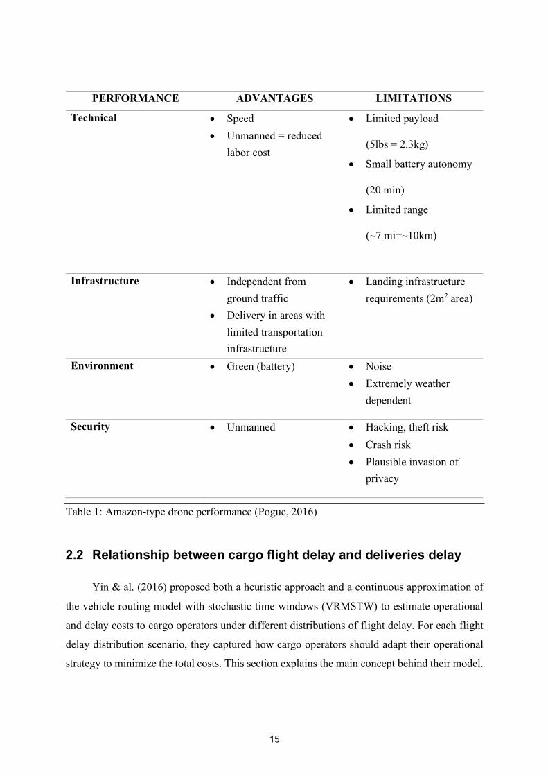
PERFORMANCE ADVANTAGES LIMITATIONS
Technical • Speed • Unmanned = reduced
labor cost
• Limited payload
(5lbs = 2.3kg)
• Small battery autonomy
(20 min)
• Limited range
(~7 mi=~10km)
Infrastructure • Independent from ground traffic
• Delivery in areas with limited transportation infrastructure
• Landing infrastructure requirements (2m2 area)
Environment • Green (battery) • Noise • Extremely weather
dependent
Security • Unmanned • Hacking, theft risk • Crash risk • Plausible invasion of
privacy
Table 1: Amazon-type drone performance (Pogue, 2016)
2.2 Relationship between cargo flight delay and deliveries delay
Yin & al. (2016) proposed both a heuristic approach and a continuous approximation of
the vehicle routing model with stochastic time windows (VRMSTW) to estimate operational
and delay costs to cargo operators under different distributions of flight delay. For each flight
delay distribution scenario, they captured how cargo operators should adapt their operational
strategy to minimize the total costs. This section explains the main concept behind their model.
16
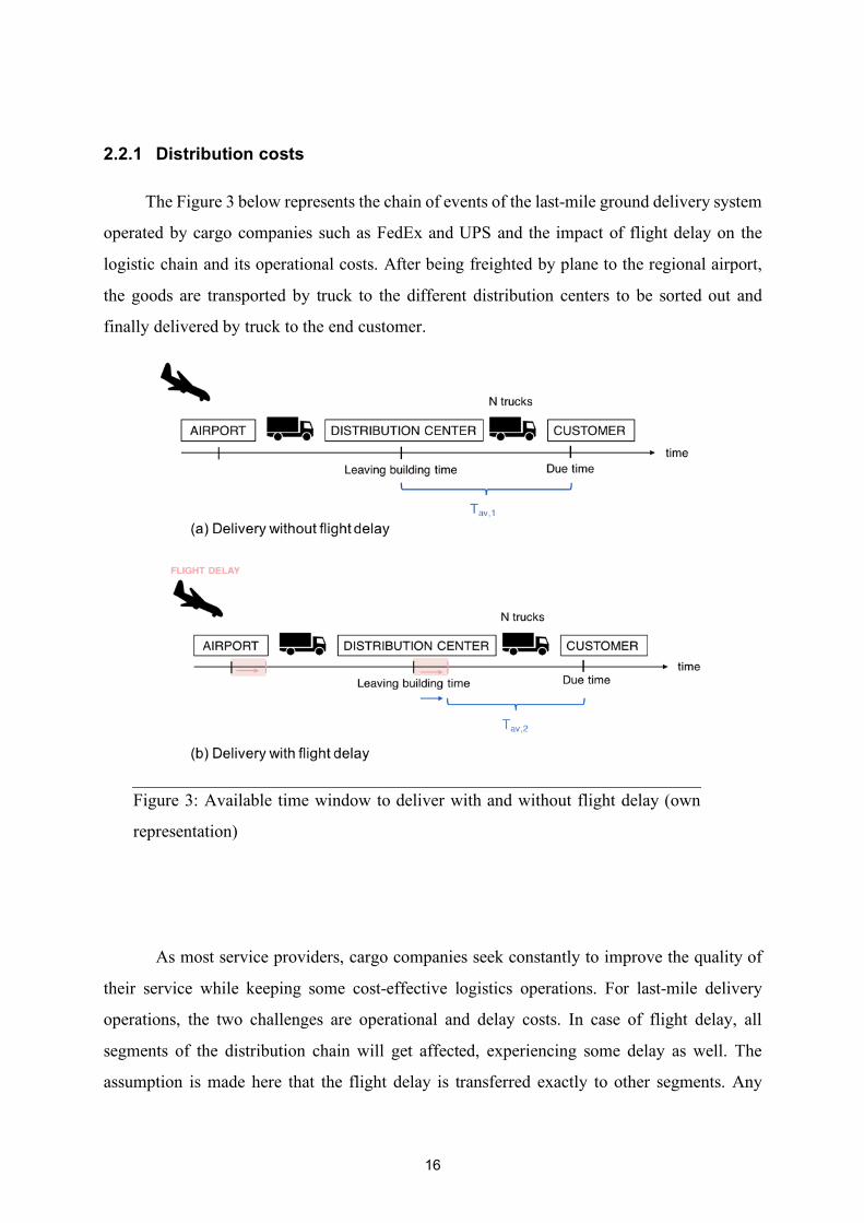
2.2.1 Distribution costs
The Figure 3 below represents the chain of events of the last-mile ground delivery system
operated by cargo companies such as FedEx and UPS and the impact of flight delay on the
logistic chain and its operational costs. After being freighted by plane to the regional airport,
the goods are transported by truck to the different distribution centers to be sorted out and
finally delivered by truck to the end customer.
As most service providers, cargo companies seek constantly to improve the quality of
their service while keeping some cost-effective logistics operations. For last-mile delivery
operations, the two challenges are operational and delay costs. In case of flight delay, all
segments of the distribution chain will get affected, experiencing some delay as well. The
assumption is made here that the flight delay is transferred exactly to other segments. Any
Figure 3: Available time window to deliver with and without flight delay (own
representation)

17
additional gain or loss of time due to packages sorting or traffic is neglected. The last segment
of the distribution chain (from the distribution center to the end-customer) experiences some
time pressure as the initial time-window available Tav,1 to deliver all parcels on time is reduced
to Tav,2 (Figure 3). If the companies keep the same size of the truck fleet, some packages will
not be delivered on time. This will induce some delay costs as customers can ask for a full
refund for any late delivery and will get disappointed by the service. In a flight delay situation,
cargo companies have one option to limit their delay costs: increasing the size of their truck
fleet. They will be able to deliver the parcels faster and thus on time. However, this method
induces more trucks and drivers and thus more operational costs. Hence, to minimize the
distribution costs, operators must find a trade-off between operational and delay costs:
Operational costs:
• Veh-based operational costs [$/truck]
• Mile-based operational costs [$/mile]
Delay costs:
• Late delivery costs [$/late delivery]
• Lateness costs [$/hour of lateness]

18
2.2.2 Stochastic flight delay
Flight delay is a stochastic phenomenon which leads to a stochastic arrival of trucks to
the local distribution center and thus to a stochastic available time window to deliver the
packages. As described above, the operators can adjust their strategy (size of the fleet) to cope
with the time-pressure induced by flight delay. However, a delivery strategy is a medium- or
even long-term strategy which cannot be changed daily. This means that the operators must
find an optimal strategy which must be robust enough to absorb a certain amount of delay but
which also allows a certain proportion of missed deliveries and its corresponding costs.
The approach used by Yin & al. (2016) to solve this problem is to optimize the delivery strategy
(i.e. the size of the fleet, i.e. the time-window Tp needed to deliver all packages from the time
the trucks leave the distribution center) based on the distribution of the available time windows
Tav, in order to minimize the distribution costs. The Figure 4 illustrates the link between the
costs and the distribution of available time windows. If the operator chooses a very small and
conservative time-window Tp (yellow line on the left), it means that the strategy aims for a large
fleet of trucks that can deliver all packages in a very small amount of time and so absorb even
the biggest delays. On the one hand, the delay costs will be minimal but on the other hand, due
to the numerous trucks and drivers, the operational costs will rise considerably. Moreover, the
fleet will be over-sized for most of the Tav (i.e. flight delay) scenarios. On the contrary, if the
operator chooses a very large time window Tp (yellow line on the right), it means that the
strategy aims for a very small fleet of trucks with smaller operational costs but that needs a lot
of time to deliver all parcels, leading to major delay costs. Indeed, there is a high probability
that the needed time-window T is larger than the available one Tav, causing numerous missed
deliveries. The optimal time window (i.e. size of the fleet) drawn as a red line in Figure 4.a.
will be located somewhere in the middle of those two extremes.

19
Figure 4: Illustration of the trade-off between operational costs and delay costs based on the
distribution of the available time window Tav (adapted from Yin, Hansen &Shen (2016) )
2.2.3 The impact of cargo flight delay on deliveries delay in figures
It is known that cargo flight delay leads to delayed deliveries. But which proportion of
deliveries miss their due-time per day? How much of this delay is due to cargo flight delay?
Which costs are induced by these additional delayed packages?
Yin & al. (2014) analyzed a set of proprietary delivery records from a freight auditing company
as well as flight data obtained from a FAA ASPM (Federal Aviation Administration, Aviation
Systems Performance Metrics) database. They focused on the “due to next day” packages which
are the most vulnerable to disruption caused by flight delay. The figures presented below
describe the “Priority service” delivering packages by 10:30 am.
They showed that most packages are due by 10:30 am (85%) while 6% are due by 12:00am and
8% by 4:40pm. Among the earliest packages, about 14% of them are delayed and 23% of this
delay is due to air cargo flight delay. In the major markets, these numbers can be even higher:
flight delay accounts for 22% to 38% of package delay.

20
Figure 5: Predicted percentage of package delay vs. flight delay (Yin, Liu, & Hansen, 2014)
2.2.4 Motivation for this study
The consequences of cargo flight delays on the last-mile delivery system are now clearly
identified and quantified. The next step is to find some solutions to counter these effects. As
most service providers, cargo companies constantly seek to improve the quality of their service
while keeping some cost-effective logistics operations. Concerning the last-mile delivery, a lot
of solutions to gain time are currently analyzed, from autonomous ground vehicles to droids or
unmanned aerial vehicles. This last solution is the focus of this study. The goal is to assess is a
truck-drone delivery system could be more robust to flight delays than the current traditional
truck delivery system. Could the distribution costs be decreased? Based on the vehicle routing
problem with stochastic time windows (VRPSTW) developed by Yin & al (2016), two models
will be formulated to determine the best strategy for cargo companies to apply to decrease their
total costs under different distribution of flight delay.

21

22
3 The vehicle routing problem with a combination of trucks and drones
This section presents the two vehicle routing problem with a truck-drone combination
models developed in the study. After setting the general assumptions and the methodology used,
the formulation of the models and their solution are described.
3.1 A comparison of three delivery-system concepts
Three concepts for package-delivery were considered in this work, the traditional one with
only trucks and two with a combination of drones and trucks. For each scenario, the optimal
strategy (i.e. size and zones assignment of the fleet) to minimize the distribution costs was
determined and compared one with another. In the cases where technical performances of the
drone represented a limitation for the improvement of the system with trucks only, some
minimal required technical performances were defined.
The first scenario, called Concept 0 (Figure 6a), corresponds to the traditional delivery system
with trucks serving a defined delivery area around a distribution center. The routing model with
stochastic time windows developed by Yin & al. (2016) for this scenario will serve as the basis
for the development of the two alternative models (Concepts 1 & 2) and for the comparison of
their performance.
The first alternative (Concept 1, Figure 6b) relates to the project currently being developed by
Amazon. The solution consists of single small drones delivering one (or several) parcels at a
time from the depot to the client (Pogue, 2016). The drones do not completely replace trucks
but are assigned a part of the deliveries. Which portion of these deliveries is the optimal one
will be defined with the model.
It will be shown in section 4 that the limited range (i.e. the battery autonomy) of small delivery-
drones is a big constraint for their use as delivery vehicles. The second alternative (Concept 2, Figure 6c) seeks to overcome this limitation by using trucks as launching platforms. The truck
leaves the depot with the drone “parked” on its roof. Once it has reached the assigned delivery
zone, the drone takes off from the roof to deliver its pre-loaded parcels, while the truck keeps
completing its own deliveries in the zone. By flying back and forth between the truck and the

23
customers, the drone can be reloaded with new parcels and have its battery changed by the
driver of the truck, till all deliveries of the zone are completed. UPS realized its first residential
drone delivery with this concept in February 2017 (Kastrenakes, 2017).
a) b)
c)
Figure 6: Drone delivery concepts (own representation)
a) Concept 0: Trucks only b) Concept 1: Trucks and drones launched from the depot
c) Concept 2: Trucks and drones launched from the trucks
3.2 General assumptions
The assumptions used in the models are based on previous research. First, the design of the
delivery region into zones assigned to each vehicle follows the research of Langevin & Soumis
(1989). Furthermore, the models 1 and 2 incorporating drones in the delivery process are an
adaptation of the vehicle routing model (model 0) with stochastic time-windows (VRPSTW)
developed by Yin & al. (2016). Whereas some new assumptions were made for the introduction
of drones in the concepts 1 and 2, the basic assumptions are similar to the ones made by Yin &
al. (2016) for model 0.

24
3.2.1 Geometry of the delivery area
The delivery area is modelled as a circle centered around a sorting center and partitioned into
zones assigned to each vehicle (Figure 7a).
• The region of radius 𝑅 contains 𝑖 rings, which are divided into zones approximated as
triangles for the inner ring and as rectangles for the other rings (Figure 7b).
• Each zone, as the one shaded on the Figure 7a, has a length of 𝐿" and a width of 2𝑤" to
make one round trip during the delivery tour. As demonstrated by Newell & al. (Newell
Gordon, 1986a), 𝑤" = 8 9:;(/)
with 𝛿(𝑟) = 𝛿
• For a matter of simplification, the customer density 𝛿 (number of customer per unit area) among the delivery area is assumed under uniform distribution meaning that 𝛿 is a constant.
• The zones of a same ring are assigned to only one type of vehicles, either trucks or
drones.
Figure 7: Geometry of the delivery area and its service zones (adapted from (Yin, Hansen, &
Shen, 2016))

25
3.2.2 Delivery network
• Whereas the trucks serve the area using a radial ring road network, the drones make diagonal movements between each customer location as they fly. Their service routes are shown in the Figure 7c.
• Each zone is served by one vehicle, drone or truck, and each vehicle is assigned to a unique zone. Thus, each vehicle makes one and only round trip from the depot.
3.2.3 Delivery timing
• To simplify the analysis, a one-to-one correspondence between the flight delay and the time window change for the last-mile delivery segment from the depot to the end-customer is assumed. We do not consider any other delay that can occur during the parcel-handling or sorting, or due to traffic congestion if the delivery time was shifted in the morning peak-hour because of the delay.
• The time window Tp is defined as the time between the departure of the vehicle from the depot and the time it completes its last delivery in the assigned zone. It is the time needed by the truck to deliver all customers of its assigned zone.
• The available time-window Tav is the time between the departure of the vehicle from the depot and the delivery time asked by the customer. It is the time available for the truck to deliver all customers of its assigned zone on time.
• If the vehicle is to complete all its deliveries on time (i.e. late deliveries are unacceptable), the time window must be equal or smaller than the available time window Tp ≤ Tav.
3.3 Methodology: the grid search method
The three models were formulated based on the grid-search method and then coded in
Python. With defined input parameters, they give the best strategy in term of fleet size to
minimize total costs under different distributions of available time windows.
A vehicle routing problem (VRP) model for the concept 0 was established by Yin & al. (2016).
They used two different approaches for the optimization problem: a grid-search method and a
nonlinear mixed integer programming (MIP) formulation. Although the MIP formulation is
more exact (and more complex) than the grid-search method, they demonstrated that the results

26
given by the two approaches were very similar. Therefore, the simpler grid-search method was
chosen to develop the new VRP models for concepts 1 and 2.
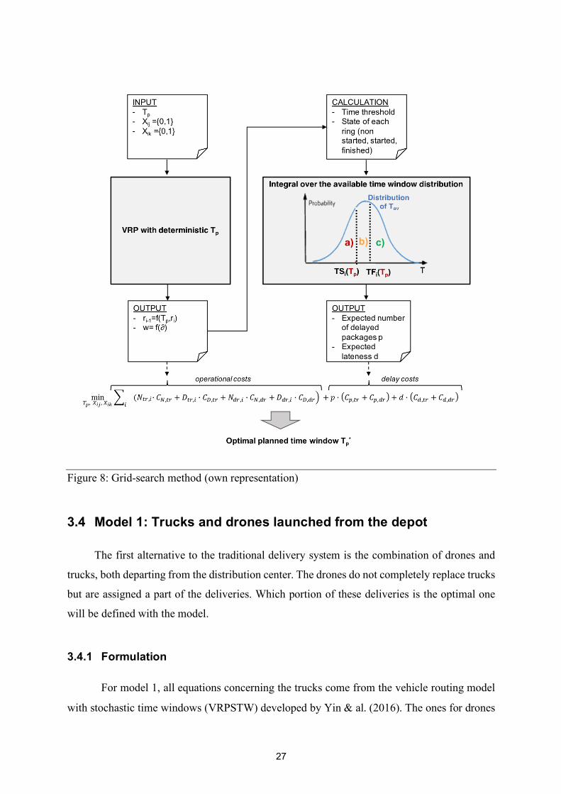
The grid-search method (Figure 8) developed by Yin & al. (2016) consists of first, resolving
the deterministic VRP for different planned time-windows Tp. The “planned time window”
refers to the aimed time window within which the operator wants to be able to complete all
deliveries. For each planned time widow Tp, the configuration of the service area (e.g. the radial
distance Li of the rings and the size of each delivery zone) which minimizes the total number
of vehicles (e.g. the total travelled distance) is calculated. Then, based on this geometry, the
associated number of delayed packages p and the total lateness d are calculated under different
distributions of the available time window Tav (e.g. actual available time window, depending
on the amount of flight delay). Thus, the total daily costs (operational and delay costs) for each
planned time window Tp can be determined. The optimal planned time window Tp* will be the
one which minimizes the total delivery costs.
27
Figure 8: Grid-search method (own representation)
3.4 Model 1: Trucks and drones launched from the depot
The first alternative to the traditional delivery system is the combination of drones and
trucks, both departing from the distribution center. The drones do not completely replace trucks
but are assigned a part of the deliveries. Which portion of these deliveries is the optimal one
will be defined with the model.
3.4.1 Formulation
For model 1, all equations concerning the trucks come from the vehicle routing model
with stochastic time windows (VRPSTW) developed by Yin & al. (2016). The ones for drones

28
were developed for this study. They are all summarized below with the equations concerning
drones. All notations used in the formulation of models are listed in the section “List of
Notations” on the pages viii and ix.
For one vehicle serving one zone in the ith ring:
1) The local (in the service zone) travelled distance is:
𝐷#/,"$%&'$ = 𝜕𝐴"BC9+ 2𝐿" (1)
𝐷0/,"$%&'$ = 𝜕𝐴"8EBC9F:+ E G
BC;F: (2)
Where 𝐴" = 2𝜔"𝐿" is the area of a zone of the ring i. These equations are based on the
rectangular approximation of the service zone, and the fact that the traverse distance between
two uniformly distributed customers is BC9
.
2) The line-haul (from the depot to the service zone) travelled distance is:
𝐷#/,"$ = 𝐷0/,"$ = 𝑟"HG (3)
3) The total stop time needed to serve customers in the zone is:
𝑆#/," = 𝜕𝐴"𝜏#/ (4)
𝑆0/," = 𝜕𝐴"𝜏0/ (5)
The optimization problem can be formulated as:
minNO,PCQ,PCR
S [𝑋"V(𝑁#/,"∙ 𝐶,,#/ + 𝐷#/," ∙ 𝐶1,#/) + 𝑋"Y(𝑁0/," ∙ 𝐶,,0/ + 𝐷0/," ∙ 𝐶1,0/)
"]
+𝐶2 ∙ (𝑝#/ + 𝑝0/) + 𝐶$ ∙ (𝑑#/ + 𝑑0/) (6)
s. t. 𝑋"V ∙ E1C,`ab a
+ 𝐴"𝛿 ∙ 𝜏#/F ≤ 𝑇2 (7)
𝑋"Y ∙ E1C,eabea
+ 𝐴"𝛿 ∙ 𝜏0/F ≤ 𝑇2 (8)
𝑋"Y ∙ 𝐷0/,",f%gh ≤ 2 ∙ 𝐷i'j (9)
𝑋"Y ∙ 𝐴"𝛿𝑤 ≤ 𝑊i'j (10)

29
∑ (𝑋"V + 𝑋"Y) ∙ 𝐿"" = 𝑅 (11) 𝑋"mG,V ≤ maxp𝑋"V, 𝑋"Yq (12) 𝑋"mG,Y ≤ maxp𝑋"V, 𝑋"Yq (13) {𝑋"V , 𝑋"Y} ∈ {0; 1} (14)
𝐿" ≥ 0 (15)
The objective function (6) aims at minimizing the total costs. The set of independent decision
variables are Tp, Xij and Xjk where Xij and Xjk are some binary variables that define if a ring i is
served by trucks (Xij =1) or by drones (Xik =1). All the other variables can be derive from these
variables. The first term ∑ (𝑁#/,"∙ 𝐶,,#/ + 𝐷#/," ∙ 𝐶1,#/ + 𝑁0/," ∙ 𝐶,,0/ + 𝐷0/," ∙ 𝐶1,0/)"
represents the operational costs (vehicle-based costs 𝐶,,#/ and mile-based costs 𝐶1,#/)
depending on the number of trucks and drones. The second term 𝑝 ∙ p𝐶2,#/ + 𝐶2,0/q + 𝑑 ∙
p𝐶0,#/ + 𝐶0,0/q represents the delay costs (missed deliveries and lateness). Equations (7) and
(8) define the time-window constraint. The time needed by each driver or drone to deliver all
parcels in its delivery zone (travelling time plus service time) must be smaller than the aimed
time-window Tp (called “planned time-window”) fixed by the company strategy. The drones
are subject to two more constraints: a maximum range constraint 2 ∙ 𝐷i'j (9) due to the
limitation of the battery autonomy as well as a maximum payload constraint 𝑊i'j(10).
Equation (11) specifies that the sum of lengths Li of all rings must be equal to the radius R of
the global delivery region. Equations (12) and (13) prevent any holes in the system. If a ring i
is not served by either some trucks nor some drones, the next rings will not be served either.
3.4.2 Solution
For the rings served by trucks, Yin & al. found the solution to the optimization problem of the
VRP. For rings served by drones, the main results are summarized below. By testing the models
with numerical values, the results showed that the drones are quickly limited by their range and
cannot even reach the second ring of the optimal truck delivery system (model 0). Thus, to
simplify the model, it was decided to ignore the binary variables Xij and Xjk in the model.
Instead, the maximum distance the drones can reach in the delivery region is defined and the

30
trucks are set to deliver the rest of the delivery region beyond this point. As a consequence, the
objective function (6) has now only one independent decision variable, Tp.
1) For i ≥ 1, the widths of each service zone are equal. Yin & al. showed that although the central ring is approximated as a triangle and not a rectangle, it may not need to be differentiated due to its small size in most cases. Thus, the width of each zone in a ring i is:
𝜔" = 8 9:;
(16)
2) The radial distance between the different rings can be found recursively by starting by
the outer ring R of the delivery region:
𝑟#/,"HG =p9m√z;{bq·/CHN·b
:m√z;{b (17)
𝑟0/,"HG = max(𝑟"HGN , 𝑟"HG1}~�, 𝑟"HG� ) (18)
with: 𝑟0/,"HGN = N·beaH/C(√�m√z;{eabea)GH√�H√z;{eabea
(19)
𝑟0/,"HG1}~� =
1����aC√�
:H√� (20)
𝑟0/,"HG� = /C√z;�H�}~�√z;�
(21)
and: 𝑟0/,"HGN ≤ 𝑇 · 𝑉0/ (22)
𝑟0/,"HG� ≤ 1}~�:
(23)
3) Number of vehicles needed in the 𝑖#� ring (regardless of whether it is served by trucks
or drones):
𝑁" =�paC���aCq
�B
(24)
For the second part of the objective function which relates to the delay costs, the number of late
deliveries 𝑝 and the amount of lateness 𝑑 are defined based on the distribution of available time
windows. First, a time threshold (equations (25) to (30)) is defined to evaluate in which state
each ring (and thus each delivery zone) is. There are three states illustrated on the Figure 9. If
a ring cannot be started (state a), it means that all deliveries due on this ring will be late and the

31
total lateness for a zone will be equal to the number of customers in this zone times the average
lateness of a delivery. If a ring cannot be finished (state b), only a part of the deliveries can be
completed on time. To finish with, if a ring can be finished (state c), all deliveries are on time,
meaning that there is no late deliveries nor lateness.
Equations (31) to (39) below give the number of late deliveries and the amount of lateness for
each scenario.
Figure 9: The three possible states of a ring (Yin, Hansen, & Shen, 2016)
4) The time needed to finish the first ring is:
𝑇�G,#/ = �:��m:B���;·
��B�
b a� + 2𝜔G𝐿G𝛿𝜏#/ (25)
𝑇�G,0/ = :B���;bea
8EB�9F:+E G
;B�F:+ 2𝜔G𝐿G𝜏0/ (26)
5) The time needed to start the ith ring (1 ≥ i ≥ K) is:
𝑇#/,"� = 𝑇#/,"HG� + �C��b
(27)
𝑇0/,"� = ∑ E �QbeaF"HG
V�G = 𝑇0/,"HG� + �C��bea
(28)
6) The time needed to finish the ith ring (1 ≥ i ≥ K) is:

32
𝑇#/,"� = 𝑇#/,"HG� +(:�CH�C��)m:BC�C;·
��BCH:BC���C��;·
��BC��
b a+(2𝜔"𝐿"𝛿𝜏#/ − 2𝜔"HG𝐿" − 1𝛿𝜏#/) (29)
𝑇0/,"� = 𝑇0/,"HG� + :BC�C;bea
8EBC9F:+E G
;BCF:+ 2𝜔"𝐿"𝜏0/ (30)
7) The number of late packages is:
• If the ring is in state a (Tp ≤ T�� i.e. the ring cannot be started):
𝑝#/,"' = 𝑝0/,"' = 2𝐿"𝜔"𝛿 · :�E∑ �QC��
Q�� m���CF
:BC (31)
• If the ring is in state b (T�� ≤ Tp ≤ T�� i.e. the ring cannot be finished):
𝑝#/,"� = � ;(NC�HN~ )
�¡`a
m¢£C�
�¡`am{`a;BC
¤ · �:�·∑ (�QC��
Q�� m���C)
:BC� (32)
𝑝0/,"� =
⎝
⎜⎛ ;(NC
�HN~ )
¢¡ea
¨E£C� F�m© �
¢£Cª�m;{ea
⎠
⎟⎞· �
:�·∑ (�QC��Q�� m���C)
:BC� (33)
• If the ring is in state c (T�� ≤ Tp ≤ T�� i.e. the ring cannot be finished):
𝑝#/,"& = 𝑝0/,"& = 0 (34)
8) The amount of lateness is: • If the ring is in state a (Tp ≤ T�� i.e. the ring cannot be started):
𝑑#/,"' = 𝑝#/,"' · ©pN a,C
® HN~ mN a,C� HN~ q
:ª (35)
𝑑0/,"' = 𝑝#/,"' · ©pNea,C
® HN~ mNea,C� HN~ q
:ª (36)
• If the ring is in state b (T�� ≤ Tp ≤ T�� i.e. the ring cannot be finished):
𝑑#/,"� = 𝑝#/,"� · ©N a,C� HN~ :
ª (37)
𝑑0/,"� = 𝑝0/,"� · ©Nea,C� HN~ :
ª (38)
• If the ring is in state c (T�� ≤ Tp) i.e. the ring can be finished):
𝑑#/,"& = 𝑑0/,"& = 0 (39)

33
Finally, the total expected number of late deliveries and the total expected amount of lateness
can be obtained by calculating the numerical integral of equations (31) to (39) over the
probability of the available time window P(Tav).
𝑝 = ∑ ©∫ 𝑝#/,"' · 𝑃(𝑇'±)𝑑T²³ +∫ 𝑝#/,"� · 𝑃(𝑇'±)𝑑T²³#�´�CN~ �N®C
N®CN~ �µ
ª +"
∑ ©∫ 𝑝0/,"' · 𝑃(𝑇'±)𝑑T²³ +∫ 𝑝0/,"� · 𝑃(𝑇'±)𝑑T²³#�´�CN~ �N®C
N®CN~ �µ
ª" (40)
𝑑 = ∑ ©∫ 𝑑#/,"' · 𝑃(𝑇'±)𝑑T²³ +∫ 𝑑#/,"� · 𝑃(𝑇'±)𝑑T²³#�´�CN~ �N®C
N®CN~ �µ
ª" +
∑ ©∫ 𝑝0/,"' · 𝑃(𝑇'±)𝑑T²³ +∫ 𝑝0/,"� · 𝑃(𝑇'±)𝑑T²³#�´�CN~ �N®C
N®CN~ �µ
ª" (41)
3.5 Model 2: Trucks and drones launched from the trucks
In the model 2, a truck and a drone work as a pair (Figure 6c). The truck driver leaves
the depot with the drone “parked” on the roof of the truck. Once it has reached the assigned
delivery zone, the drone will take off to deliver its pre-loaded parcels. During this time, the
truck driver keeps delivering its own parcels. When the drone is done with its deliveries, it
meets again with the truck at a customer’s place. After the landing of the drone on the roof, the
truck driver can reload the drone with new parcels and change its battery if necessary. This
process goes on till all deliveries have been completed. The truck and the drone meet one last
time before going back to the distribution centre.
3.5.1 Additional assumptions
Some additional assumptions from the ones described in section 3.2 apply for model 2.
• The truck and the drone always meet at a customer’s place which was assigned to the
truck.
• The duration between the take-off of the drone from the roof of the truck and the time
it lands again on it is called a loop (Figure 10). The pair repeats the same loops (each
vehicle serves the same number of customers per loop) during the whole service of the
zone. Each loop of the drone is subject to the same three constraints as the ones in the

34
first model: the time window 𝑇2 , the maximum payload 𝑊i'j and the maximum range
𝐷i'jconstraints.
Figure 10: Illustration of one truck-drone loop in the delivery region (own representation)
3.5.2 Formulation
1) The travel time per loop in a zone of the 𝑖#� ring is:
𝑇#/,"$%%2 = #𝑐𝑢𝑠𝑡0/ ∙
Gb a∙B∙;
+ #𝑐𝑢𝑠𝑡#/ �E£�m
�£∙¢F
b a+ 𝜏#/� (42)
𝑇0/,"$%%2 = #𝑐𝑢𝑠𝑡#/ ∙
E£�m�
£∙¢F
bea+ #𝑐𝑢𝑠𝑡0/ »
8£�¼ m
�£�∙¢�
bea+ 𝜏0/½ (43)
Where #𝑐𝑢𝑠𝑡#/ = and #𝑐𝑢𝑠𝑡0/are the number of customers served respectively by the truck
and the drone during one loop.
2) The number of loops during which a drone can fly before changing the battery is:
𝑁$%%2¾,0/�'##h/¿ = 𝑖𝑛𝑡 ©Á'gÂh
bea∙ GòÄ(NÅÆÆO,`aH{`a;NÅÆÆO,ea)
ª (44)
3) The total number of loops needed to deliver the entire assigned zone is:
𝑁$%%2¾ = 𝑖𝑛𝑡 E ÇC∙;#&Ⱦ#`am#&Ⱦ#ea
F (45)
The optimization problem of the VRP model is the same as the one from model 0 explained by
Yin & al. (2016) in their research, with the additional constraints (49) to (54). The goal again
is to minimize the number of vehicle pairs (e.g. the total travelled distance).

35
minNO
∑ [(𝑁#/,"∙ 𝐶,,#/ + 𝐷#/," ∙ 𝐶1,#/) + (𝑁0/," ∙ 𝐶,,0/ + 𝐷0/," ∙ 𝐶1,0/)" ] (46)
+𝐶2 ∙ (𝑝#/ + 𝑝0/) + 𝐶$ ∙ (𝑑#/ + 𝑑0/)
s.t 𝑡"$"ghH�'È$ + 𝑡"$%&'$ + 𝑆" ≤ 𝑇2 (47)
∑ 𝐿"" = 𝑅 (48)
#𝑐𝑢𝑠𝑡0/ ≤�}~��
(49)
𝑇0/,"$%%2 ≤ ɲÊËÌ
ÍÎÏ (50)
𝑇0/,"$%%2 ≤ TÐ (51)
𝑇#/,"$%%2 ≤ TÐ (52)
𝑇#/,"$%%2 − 𝜏#/ ≤
Á'gÂhb a
(53)
𝑇#/,"$%%2, 𝑇0/,"
$%%2, #𝑐𝑢𝑠𝑡0/, #𝑐𝑢𝑠𝑡#/ ≥ 0 (54)
The objective function (46) is the same as the model 1 without any binary variables as all rings
re served by both trucks and drones. The equation (49) limits the number of customers that a
drone can serve within one loop due to the maximum payload Wmax that the drone can carry.
The equations (50) to (53) specify that the duration of one loop must not exceed the planned
time window nor the maximum range for drones.
3.5.3 Solution
The solutions of the optimization problem are presented below:
1) For i ≥ 1, the widths of each service zone are equal. Yin & al. showed that although the central ring is approximated as a triangle and not a rectangle, it may not need to be differentiated due to its small size in most cases. Thus, the width of each zone of the 𝑖#� ring is:
𝜔" = 8 9:;
(55)
2) The number of customers served by each drone and each truck within one loop in a service zone is:
#𝑐𝑢𝑠𝑡0/ =Ñ����
(56)

36
with: #𝑐𝑢𝑠𝑡0/ ≤ Ò���
8£�¼ m
�£�∙¢�
m{ea∙bea (57)
#𝑐𝑢𝑠𝑡0/ ≤ ÓÔ∙bea
8£�¼ m
�£�∙¢�
m{ea∙bea (58)
#𝑐𝑢𝑠𝑡0/ ≤ TÐ ∙ 𝑉#/ ∙ 𝜔 ∙ 𝛿 (59)
#𝑐𝑢𝑠𝑡#/ = min(#𝑐𝑢𝑠𝑡#/(�µ), #𝑐𝑢𝑠𝑡#/
(�G), #𝑐𝑢𝑠𝑡#/(�:), #𝑐𝑢𝑠𝑡#/
(�9)) (60)
with: #𝑐𝑢𝑠𝑡#/(�µ) =
1}~�H#&Ⱦ#ea�8£�¼ m
�£�∙¢�
∗m{ea∙bea�
8£�¼ m
�£�∙¢�
(61)
#𝑐𝑢𝑠𝑡#/(�G) =
NO∙beaH#&Ⱦ#ea�8£�¼ m
�£�∙¢�
∗m{ea∙bea�
8£�¼ m
�£�∙¢�
(62)
#𝑐𝑢𝑠𝑡#/(�:) =
NO∙b aH#Ö×Ø`ea£∙¢
£�m
�£∙¢m{`a∙b a
(63)
#𝑐𝑢𝑠𝑡#/(�9) =
#&Ⱦ#ea
⎝
⎜⎛¨£
�¼ � �
£�∙¢�¡ea
m{eaH�
¡`a∙£∙¢
⎠
⎟⎞m{`a
£��
�£∙¢
¡`am{`aH
¨£�¼ � �
£�∙¢�¡ea
(64)
3) The radial distance between the different rings can be found recursively by starting by
the outer ring R of the delivery region:
𝑟"HG =NOmÙH/CÚ
�£¢#Ö×Ø``a�#Ö×Ø`ea
»i'jEpNÅÆÆO,`aH{`aq,NÅÆÆO,eaFmÙmÛ·Ü}~�
¡ea·}~�©EÝÅÆÆO,`a�Þ`aF,ÝÅÆÆO,eaª½ß
�¡`a
H �£¢#Ö×Ø``a�#Ö×Ø`ea
»i'jEpNÅÆÆO,`aH{`aq,NÅÆÆO,eaFmÙmÛ·Ü}~�
¡ea·}~�©EÝÅÆÆO,`a�Þ`aF,ÝÅÆÆO,eaª½
(65)
with
r� ≤ (𝑇2 + 𝛼) · 𝑉#/ (66)
4) The number of vehicles needed in the 𝑖#�ring is:
𝑁",#/ = 𝑁",0/ =�paC���aCq
�B
(67)

37
5) The time needed to finish the first ring is:
𝑇�G =:B;��
#&Ⱦ#`am#&Ⱦ#ea�𝑚𝑎𝑥 Ep𝑇$%%2,#/ − 𝜏#/q, 𝑇$%%2,0/F + 𝛼 +
å·1}~�
bea·i'jEpNÅÆÆO,`aH{`aq,NÅÆÆO,eaF� − 𝛼 (68)
6) The time needed to start the ith ring (1 ≥ i ≥ K) is:
𝑇"� = 𝑇"HG� + �C��b a
(69)
7) The time needed to finish the ith ring (1 ≥ i ≥ K) is:
𝑇"� = 𝑇"HG� + 2𝜔𝛿𝐿𝑖#𝑐𝑢𝑠𝑡𝑡𝑟+#𝑐𝑢𝑠𝑡𝑑𝑟
�𝑚𝑎𝑥 Ep𝑇𝑙𝑜𝑜𝑝,𝑡𝑟 − 𝜏𝑡𝑟q, 𝑇𝑙𝑜𝑜𝑝,𝑑𝑟F + 𝛼 +𝛽·𝐷𝑚𝑎𝑥
𝑉𝑑𝑟·𝑚𝑎𝑥Ep𝑇𝑙𝑜𝑜𝑝,𝑡𝑟−𝜏𝑡𝑟q,𝑇𝑙𝑜𝑜𝑝,𝑑𝑟F� − 𝛼 (70)
8) The number of late packages for each truck and drone serving a zone in the ith ring is:
• If the ring is in state a (Tp ≤ T�� i.e. the ring cannot be started):
𝑝"' = 𝑝0/,"' = 2𝐿"𝜔"𝛿 · :�E∑ �QC��
Q�� m���CF
:BC (71)
• If the ring is in state b (T�� ≤ Tp ≤ T�� i.e. the ring cannot be finished):
𝑝"� =
⎝
⎜⎛ (NC
�HN~ mÙ)·(#𝑐𝑢𝑠𝑡𝑡𝑟+#𝑐𝑢𝑠𝑡𝑑𝑟)
2𝜔𝛿𝐿𝑖#𝑐𝑢𝑠𝑡𝑡𝑟+#𝑐𝑢𝑠𝑡𝑑𝑟
»𝑚𝑎𝑥Ep𝑇𝑙𝑜𝑜𝑝,𝑡𝑟−𝜏𝑡𝑟q,𝑇𝑙𝑜𝑜𝑝,𝑑𝑟F+𝛼+𝛽·𝐷𝑚𝑎𝑥
𝑉𝑑𝑟·𝑚𝑎𝑥©E𝑇𝑙𝑜𝑜𝑝,𝑡𝑟−𝜏𝑡𝑟F,𝑇𝑙𝑜𝑜𝑝,𝑑𝑟ª½⎠
⎟⎞· �
:�·∑ (�QC��Q�� m���C)
:BC� (72)
• If the ring is in state c (T�� ≤ Tp ≤ T�� i.e. the ring cannot be finished):
𝑝"& = 0 (73)
9) The amount of lateness is: • If the ring is in state a (Tp ≤ T�� i.e. the ring cannot be started):
𝑑"' = 𝑝"' · ©pNC
®HN~ mNC�HN~ q
:ª (74)
• If the ring is in state b (T�� ≤ Tp ≤ T�� i.e. the ring cannot be finished):
𝑑"� = 𝑝"� · ©N a,C� HN~ :
ª (75)

38
• If the ring is in state c (T�� ≤ Tp) i.e. the ring can be finished):
𝑑"& = 0 (76)
Finally, the total expected number of late deliveries and the total expected amount of lateness
can be obtained by calculating the numerical integral of equations (71) to (76) over the
probability of the available time window P(Tav).
𝑝 = ∑ ©∫ 𝑝"' · 𝑃(𝑇'±)𝑑T²³ +∫ 𝑝"� · 𝑃(𝑇'±)𝑑T²³#�´�CN~ �N®C
N®CN~ �µ
ª" (77)
𝑑 = ∑ ©∫ 𝑑"' · 𝑃(𝑇'±)𝑑T²³ +∫ 𝑑"� · 𝑃(𝑇'±)𝑑T²³#�´�CN~ �N®C
N®CN~ �µ
ª" (78)

39

40
4 Results In this section, the empirical results found by the application of the models are presented.
The three delivery concepts are tested and compared with the estimated medium-term vision of
the technical performances of the delivery-drones.
4.1 Input parameters
The numerical values for the inputs parameters were gathered based on the work of Yin
& al (2016), different interviews of UAV systems researchers, as well as different articles on
UAVs ((Pogue, 2016), (Ric, 2015)). They are summarized in the Table 2 below.
VEHICLE INPUTS
Drone Truck
Speed Vdr = 50 mph Vtr = 30 mph
Handling time per
delivery tdr = 0.008 h (0.5min) ttr = 0.025 h (1.5 min)
Parcel loading time a = 0.025 h (1.5 min) -
Battery replacement time b = 0.025 h (1.5 min) -
Range (back and forth) Dmax =10 mi -
Maximum payload Wmax = 10 lbs (4.5kg) -
Avg weight of a parcel 𝑤= 2.5 lbs (1.1kg) -
Launch point - R_min_dr = 0 mi
Veh-based cost 𝐶,,0/ = 2.5 $/veh/day 𝐶,,#/ = 15 $/veh/day
Mile-based cost 𝐶1,0/ = 0.03 $/veh/mi 𝐶1,#/ = 1.5 $/veh/mi
Cost per missed delivery 𝐶2 = 60 $/delivery 𝐶2 = 60 $/delivery

41
Cost per hour of lateness 𝐶$ = 6 $/h 𝐶$ = 6 $/h
SERVICE AREA INPUTS
Customer density ∂ = 0.8 customer/mi2
Radius of the service area R = 30 mi
Offset offset = 1
Table 2: Input parameters
4.1.1 Characteristics of drones
This study aims at assessing the future situation (in a 10 to 15-year vision) of delivery
drones, by estimating the potential evolution of the technical performances of drones. The
current ones were summed up in the Table 1 (section 2.1.2).
Increasing the range and the payload capacity of the drone strongly depends on the
improvements of battery capacity as it defines the amount of power available to generate the
propeller thrust required to counter the force of gravity and move forward (Ric, 2015). The
longer range and heavier payload capacity are wanted, the more powerful and therefore bigger
and heavier the battery must be. To carry this heavier total weight the battery must be more
powerful and so on in a vicious circle. The challenge here is to build batteries that are at the
same time small and powerful. There is for instance some active research on hydrogen fuel
cells, which could offer a cheaper, greener and less noisy alternative to internal combustion
vehicles and a lighter and more autonomous one to batteries (Plaza, 2017). However, the
research must still overcome some challenges such as the inefficiency of producing,
transporting and storing hydrogen and the high costs of the technology (Romm, 2014). Based
on this information, it was decided that in a 15-year-vision, the range could possibly increase
from 6 to 10 mi (round-trip), the payload capacity from 5 to 10 lbs, and the speed from 40 to
50 mph. Moreover, it was assumed that the delivery-UAV will by then be able to carry and
deliver several packages in one single flight. Concerning the weight of the parcels, Amazon’s
vice president Paul Misener claimed that 86% of Amazon’s packages weigh less than 5 lbs

42
(Pogue, 2016). Among those packages, an average weight per parcel of 2.5 lbs was estimated.
This value is quite uncertain and will be tested with a sensitivity analysis in section 5. However,
the important parameter is not really the weight of a parcel or the maximum payload a drone
can carry but rather their ratio, i.e how many parcels a drone can carry simultaneously. For the
first tests of the models, this number is equal to four parcels.
4.1.2 Costs
The delay costs Cp and Cl as well as the operational costs for trucks are the same used by Yin
& al. in their study (2016). The vehicle-based costs include a base salary for the driver, the
initial investment costs for the acquisition of the vehicle as well as the maintenance and
insurance costs. A initial investment cost of 40’000$ with a life-span of 10 years were
estimated. The mile-based costs include the fuel costs and the driver’s salary per mile.
Concerning the drones, the vehicle-based costs were defined based on an estimation made by
Zhiwei & al. (2014). They assumed an initial investment (maintenance included) of 4’000$ for
a life-span of 5 years and no driver costs. The mile-based costs were calculated based on the
work of D’Andrea (2014), in which he calculated the costs related to energy and power for a
potential delivery drone.
4.1.3 Flight delay and time window distribution
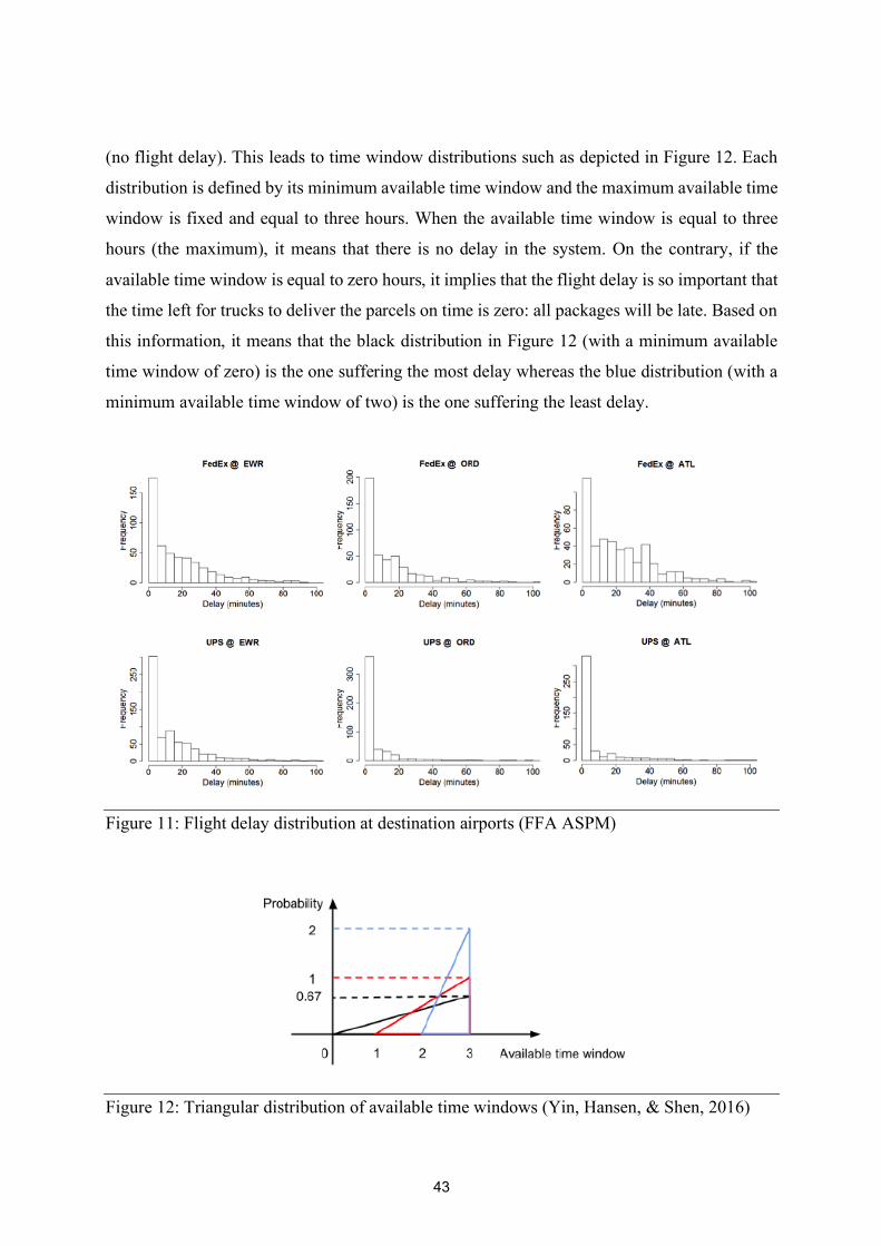
To define the type of distribution for the available time window Tav, Yin & al. (2016) gathered
some delay data from the FAA ASPM (Federal Aviation Administration, Aviation Systems
Performance Metrics) individual flight database. They analyzed the flight delay of two leading
cargo operators, FedEx and UPS at three important airports (Atlanta, Newark and Orlando) and
collected the 2012 FedEx overnight flights and the 2013 UPS flights at those airports. From
Figure 11, it is observed that most flights do not experience any delay. For the delayed flights,
their number decreases with the amount of delay. To simplify the translation of the flight delay
distribution to the available time window distribution, Yin & al. assumed a one-to-one
correspondence between the flight delay and the time window change for the last-mile delivery
segment. This assumption was maintained for the new models. They choose to approximate the
trend by a triangular distribution with a mode of 0. They accepted the fact that this
approximation works well for all flight delays expect the cases with a maximum time window
43
(no flight delay). This leads to time window distributions such as depicted in Figure 12. Each
distribution is defined by its minimum available time window and the maximum available time
window is fixed and equal to three hours. When the available time window is equal to three
hours (the maximum), it means that there is no delay in the system. On the contrary, if the
available time window is equal to zero hours, it implies that the flight delay is so important that
the time left for trucks to deliver the parcels on time is zero: all packages will be late. Based on
this information, it means that the black distribution in Figure 12 (with a minimum available
time window of zero) is the one suffering the most delay whereas the blue distribution (with a
minimum available time window of two) is the one suffering the least delay.
Figure 11: Flight delay distribution at destination airports (FFA ASPM)
Figure 12: Triangular distribution of available time windows (Yin, Hansen, & Shen, 2016)

44
4.2 Numerical results
In this section, the numerical results of the simulations with the input parameters
described in section 4.1 are presented.
4.2.1 Optimal planned time window
Figure 13 illustrates the evolution of total costs depending on the planned time window (i.e. the
strategic size of the fleet) under different available time window distributions. As it was
explained in section 4.1, the distributions are defined by their minimum available time window.
For each distribution, an optimal planned time window Tp* can be identified (coloured dots in
the Figure 13), as the one minimizing the total delivery costs. The Tp*s and their associated total
costs are gathered in Table 3.
Quite logically, the optimal planned time window increases and the costs decrease with the rise
of the minimum available time window. The less delay the system has to absorb, the larger
delivery time window (i.e. the smallest fleet) it can aims for. For the scenario with the smallest
minimum time window (i.e. highest maximum delay, represented in blue in Figure 13), the
optimal planned time window represents 56% of the no-delay optimal time window for the
models 0 and 1 with an increase factor for total costs of about 3. For model 2, the minimum
optimal planned time window is 52% of the maximum one (no-delay scenario) for a
multiplication of total costs by 3.3.
Figure 13: Total cost vs planned time windows under different available time window
distributions (own representation)

45
Min available time
Model window 0.0 0.75 1.5 2.25 3.00
Model 0 1.67
(2.39)
2.00
(1.16)
2.33
(1.11)
2.75
(0.87)
3.0
(0.77)
Model 1 1.67
(2.22)
2.00
(1.43)
2.42
(1.04)
2.83
(0.87)
3.0
(0.80)
Model 2 1.58
(1.52)
1.83
(0.88)
2.08
(0.65)
2.58
(0.53)
3.0
(0.46)
Table 3: Optimal time window Tp and (associated total costs) under different available time
window distributions (own results)
4.2.2 Optimization of the delivery system
Figure 14 shows the optimal solutions for each distribution of available time window. Whereas
the optimal time window increases with the minimum available time window (Figure 14.a) and
their relationship is rather linear, the total costs, the number of vehicles, the number of packages
and the amount of lateness decrease with the minimum available time window and their
relationship is convex (Figure 14.b to .f).
Figure 14: Optimal solutions of programing and simulation models (own results)

46
In terms of total costs, models 0 and 1 perform similarly whereas the model 2 optimizes the
system drastically, reducing the total costs of about 3’000 to 7’500 $/day under every
distribution of available time window.
To understand this difference, it is interesting to look at Figure 15, which shows the distribution
of costs between trucks and drones. With the second concept, the drones are responsible for up
to 30% of total costs under the maximum delay scenario (i.e. minimum available time window
equal to 0). This contribution decreases with the delay to reach a share of about 5% with the
no-delay scenario. With concept 1, the share of drones in total costs is close to zero. This
difference between models 1 and 2 is not surprising looking at Figure 14.c and .d. The number
of drones for the model 1 is limited to 12 vehicles and do not change with the distributions of
available time window, whereas in the model 2, the number of drones are between 40 and 110
vehicles. This means that the concept 1 with drones launched from the depot is very unefficient.
The drones do not bring any added value to the system and the number of trucks is roughly the
same as in model 0. The causes of this inefficiency will be investigated with a sensibility
analysis in section 0.
A last interesting information can be observed in Figure 16. The proportion of operational costs
for the models 0 and 1 is much smaller than the one for the model 2. Indeed, the unit operational
costs for trucks are much bigger than the one for drones (15$/veh/day vs. 2,5$/veh/day for the
vehicle-based cost and 1.5$/mi vs. 0,03$/mi for the mile-based costs). The much smaller size
Figure 15: Proportion of costs [%] associated to trucks and drones (own results)

47
of the truck fleet with the model 2 leads to a serious decrease in the opertional costs compared
to the two other models.
Figure 16: Proportion of operational and delay costs (own representation)

48
5 Sensitivity Analysis
This section aims at analyzing the reason why the performance of models 1 and 2 is so
different. Whereas the insertion of drones launched from the trucks (model 2) considerably
decreases the daily delivery costs, the drones launched form the depot do not bring any added-
value to the traditional truck delivery system. The potential impact on total costs of the technical
performances of drones (number of parcels carried simultaneously and range) are tested with a
sensibility analysis. An average delay of 0,5 hours (i.e. a minimum available time window of
1.5h) has been chosen.
5.1 Number of parcels carried simultaneously
More than the maximum payload, the interesting element for drone deliveries is the
number of packages that each vehicle can carry simultaneously, defining the number of
customers it can serve within one loop. In the results obtained in the previous section (section
4) the number was set to a maximum number of 4 parcels per loop (an average payload of 2.5lbs
per parcel for a maximum payload of 10lbs per drone).
The Figure 17 shows that for both models, the total costs do not evolve beyond a maximum
number of carried parcels of five. The same behaviour is observed for the number of trucks and
drones. This means that no matter how many parcels a drone can carry simultaneously, it faces
another limitation that prevents the improvement of the system.

49
Figure 17: Sensibility analysis for the number of parcels carried simultaneously by a drone
within one loop (own results)
5.2 Range of the drone
The other technical component limiting the performance of the drone is probably its
range. In the section 4, the estimated range for drones was set to 10 miles. A potential increase
of the range and its consequences on the total costs and on the size of the fleet are illustrated in
the Figure 18.
Unlike the number of carried parcels, the variation of the range has big consequences on the
total delivery costs, particularly for the model 1. Till a range of 45 miles, the costs decrease of
about 2’500$/day compared to the scenario with a range of 10 miles, before increasing again
and reaching a plateau at 9’400$/day (i.e. a decrease of 1’000$/day). Concerning the trucks,
with a range of 35 miles their number decreases also of about 40% compared to the model 0

50
before reching the plateau of a 25% difference. Concerning the drones, their number increases
as a high rate with the range, reaching a number of 600 drones for the highest ranges.
The model 2 is much less affected by the range improvement. This is due to that fact that the
performance of the truck-drone pair in this model does not depend so much on the range alone
but on the combination of the range oand the number of carried parcels. This assumption is
verified with the results on the Figure 19.
Figure 18: Sensibility analysis for the range of the drones (own results)
The Figure 19 illustrates the minimum delivery costs that can be obtained under each available
time window distribution and with different combinations of range and number of carried
parcels. The comparison between the figures a) and b) and a) and c) shows that an increase of
the range only (doubling to 20 miles) does not improve the system (i.e. decrease the costs) with
the concept 2. If a drone can only deliver 4 parcels at a time, no matter how long it can fly, its
loop will be over after the fourth delivery and it will be constraint to come back to the truck to
be reloaded. On the other hand, a simultaneous increase in the range and the number of carried
parcels (doubling to 20 miles and 10 parcels) does decrease the total costs. For a maximum

51
delay scenario (i.e. a minimum available time window equal to 0), these technical
improvements allow to decrease the total costs of 50% compared to the traditional truck
delivery case against 40% with a range of 10 miles and a number of parcels of 4 items. The
same improvements are observed for a scenario with an average delay of 0.5 hours (i.e. a
minimum available time window equal to 1.5).
As expected for the first model, the technical improvements have a clear impact on the
performance of the system. It finally becomes more profitable than the traditional truck delivery
system (model 0). It is particularly the case when the range is tripled to 30 miles. The daily
delivery costs can be reduced by up to 2’500 $/day. Despite these improvements, the second
model with trucks launched from the trucks always stays more profitable than the first one with
drones launched form the distribution center.
Figure 19: Optimal solutions for the toal costs under different technical performances of drones
(own results)

52
6 Conclusion
This study has shown that the insertion of drones in last-mile delivery systems can decrease
the total delivery costs. However, the optimization of the system depends on several parameters.
First, the delivery concept is of great importance. A combination of trucks and drones with
drones launched from the trucks (concept 2) is easily more profitable than a combination with
drones launched from the distribution center (concept 1). The second system can decrease the
daily delivery costs by up to 40% under specific distributions of the available time window
compared to the traditional delivery system. One of the reason is the high sensitivity to the
technical performances of drones. This is the second important element for the optimization of
the traditional delivery system with trucks. The current technical performances of drones, and
particularly the maximum range, limit drastically the performance of the system with drones
launched form the distribution center. For it to start becoming profitable, the range of the drones
should reach a minimum of 20 miles. Only then, the costs can be decreased by up to 10% under
specific distributions of the available time window. For the second concept with drones
launched from the trucks, only a simultaneous increase in the range and the number of carried
parcels by the drone can lead to an additional improvement of the system.
It is important to keep in mind that this study has several limitations due to its simplifying
assumptions. The most important one is the constant customer density within the delivery
region, which do not represent the real situation. However, the goal of this study was above all
to build the models to estimate the operational and delay costs due to flight delay with a truck-
drone delivery system. A variable customer density should be tested in further research.
Another element that was not taken into account for the feasibility of the truck-drone delivery
system is its dependency to weather conditions. It would be interesting to add a distribution
over time of bad weather in the model to consider the times of critical rain and wind conditions
preventing the use of drones.

53
To finish with, the concept of combined truck-drone deliveries will not happen before the
Federal Aviation Administration changes the regulations concerning the operation of
commercial drones in the United States. Only solid evidence on the security of drones for the
population will unlock the negotiations between the FAA and the cargo companies.

54

55
7 Reference list Asencio, M., Gros, P., & Patry, J.-J. (2010, August). Les drones tactiques à voilure tournante
dans les engagements contemporains. Recherches & documents.
Associated Press. (2016, April 4). The Guardian. Retrieved from Proposed drone regulation could clear the way for widespread US services: https://www.theguardian.com/technology/2016/apr/04/drone-faa-regulation-delivery-services
Defense Industry Daily. (2007, October). Textron buys UAV makers AAI & Aerosonde. Retrieved from Defense Industry Daily: http://www.defenseindustrydaily.com/textron-buys-uav-makers-aai-aerosonde-03968/
Harris, M. (2016, March). Near misses between drones and airplanes on the rise in US, says FAA. Retrieved from The Guardian: https://www.theguardian.com/technology/2016/mar/25/near-misses-between-drones-and-airplanes-on-the-rise-in-us-finds-faa
Kastrenakes, J. (2017, February). UPS has a delivery truck that can launch drones. Retrieved from The Verge: https://www.theverge.com/2017/2/21/14691062/ups-drone-delivery-truck-test-completed-video
Langevin, A., & Soumis, F. (1989). Design of multiple-vehicle delivery tours satisfying time constraints. Transpn. Res. 23B, 123-138.
Leswing, K. (2015, July). Amazon wants to reserve airspace for a drone highway . Retrieved from Futurism: https://futurism.com/amazon-wants-to-reserve-airspace-for-a-drone-highway/
Macdonald, C. (2017, February 21). UPS tests 'drive by' drone deliveries in Florida to drop packages at doors Read more: http://www.dailymail.co.uk/sciencetech/article-4245826/UPS-tests-drone-deliveries-Florida-eye-cost-cuts.html#ixzz53zm2sRpZ Follow us: @MailOnline on Twitter | DailyMail on Facebook . Retrieved from Daily Mail: http://www.dailymail.co.uk/sciencetech/article-4245826/UPS-tests-drone-deliveries-Florida-eye-cost-cuts.html
Mendoza, M. (2014, September 26). DHL tests drone Parcelcopter to deliver medicine in German island. Retrieved from TECH TIMES: http://www.techtimes.com/articles/16521/20140926/dhl-tests-drone-parcelcopter-to-deliver-medicine-in-german-island.htm

56
Newell Gordon, C. D. (1986a). Design of multiple-vehicle delivery tours-I: a ring radial network. Transpn. Res. 20B, 345-363.
Plaza, J. (2017, June). Will Hydrogen Fuel Cells helps drones stay in the air? Retrieved from Commercial UAV News: https://www.expouav.com/news/latest/hydrogen-fuel-cells-drones/
Pogue, D. (2016, January 18). Exclusive: Amazon reveals details about its crazy drone delivery program. Retrieved from Yahoo Finance: https://finance.yahoo.com/news/exclusive-amazon-reveals-details-about-1343951725436982.html
Romm, J. (2014, August). Tesla Trump Toyota Part II: the big problem with hydrogen fuel cell vehicles. Retrieved from Think Progress: https://thinkprogress.org/tesla-trumps-toyota-part-ii-the-big-problem-with-hydrogen-fuel-cell-vehicles-5917fec22274/
Schroth, F. (2017, February). UPS is testing residential delivery via drone & trucks. Retrieved from Drone Life: https://dronelife.com/2017/02/21/ups-is-testing-residential-delivery-via-drone-trucks/
Stern, J. (2013, December 1). Amazon Prime Air: Delivery by Drones Could Arrive As Early as 2015. Retrieved from abcNEWS: http://abcnews.go.com/Technology/amazon-prime-air-delivery-drones-arrive-early-2015/story?id=21064960
Wikipedia. (2017, September). Fuel cell. Retrieved from https://en.wikipedia.org/wiki/Fuel_cell#Efficiency_of_leading_fuel_cell_types
Yin, M., Hansen, M., & Shen, Z.-J. (2016, July). Estimating the impact of Flight Delay on Cargo Carriers' Ground Distribution Costs. World Conference on Transport Research (WCTR) 2016 Shanghai. Elsevier.
Yin, M., Liu, Y., & Hansen, M. (2014). Evaluating the impact of flight delay on cargo and overnight package delivery firms.
57
8 Appendix
8.1 Code - Python

58
8.1.1 Model 0
Summary
Name file (.py) Inputs Outputs Files used
BASE MODEL
1 Geometry_tr T
Vtr
density
handling
R
offset
R_min
print_on = False
Float
Float
Float
Float
Float
Float
Float
-
nbrings
summary_geom
table_geom
rings
radius
length
radius_minus
radius_avg
Area
density_rings
w_rings
Float
Matrix
Table
Array
Array
Array
Array
Array
Array
Array
Array
2 Nb_veh T
Vtr
density
handling
R
offset
R_min
print_on = False
Float
Float
Float
Float
Float
Float
Float
-
Nk
tot_nb_trucks
Array
Float
Geometry_tr_
3 Total_distance T
Vtr
density
handling
R
offset
R_min
print_on = False
Float
Float
Float
Float
Float
Float
Float
-
distance
tot_distance
Array
Float
Geometry_tr
Nb_veh
4 Op_costs T
Vtr
density
handling
R
Float
Float
Float
Float
Float
op_costs Float Nb_veh
Total_distance

59
offset
costperveh
costpermile
R_min
print_on = False
Float
Float
Float
Float
-
5 Main_op_costs
= SUMMARY of
the main results
from (1) to (4) =
VRP
T
Vtr
density
handling
R
offset
costperveh
costpermile
R_min
print_on = False
Float
Float
Float
Float
Float
Float
Float
Float
Float
-
op_costs
summary_all
table_all
nbrings
tot_nb_trucks
tot_distance
Float
Matrix
Table
Float
Float
Float
Geometry_tr
Nb_veh
Total_distance
Op_costs
6 Nb_late_packages T
Vtr
density
handling
R
offset
R_min
Tav
print_on = False
Float
Float
Float
Float
Float
Float
Float
Float
-
TF
TS
late_p
tot_late_packages
Array
Array
Array
Float
Geometry_tr
Nb_veh
7 Lateness T
Vtr
density
handling
R
offset
R_min
Tav
print_on = False
Float
Float
Float
Float
Float
Float
Float
Float
-
TF
TS
laten
tot_lateness
Array
Array
Array
Float
Geometry_tr
Nb_veh
8 Delay_costs T
Vtr
density
handling
R
Float
Float
Float
Float
Float
Total_delayed_packages
Total_lateness
delay_costs
total_lateness
total_delayed_packages
Float
Float
Float
Array
Array
Nb_late_packag
es
Lateness

60
offset
R_min
minTime
maxTime
costpermissdelivery
costperminlateness
print_on = False
Float
Float
Float
Float
Float
Float
-
T_av Array
9 Main_base_model
= SUMMARY of
the main results
from (1) to (8) =
VRP
T
Vtr
density
handling
R
offset
R_min
minTime
maxTime
costperveh
costpermile
costpermissdelivery
costperminlateness
Float
Float
Float
Float
Float
Float
Float
Float
Float
Float
Float
Float
Float
op_costs
summary_all
table_all
nbrings
tot_nb_trucks
tot_distance
Total_delayed_packages
Total_lateness
delay_costs total_lateness
total_delayed_packages
T_av
Float
Matrix
Table
Float
Float
Float
Float
Float
Float
Array
Array
Array
Geometry_tr
Nb_veh
Total_distance
Op_costs
Delay_costs

61
Code
• Geometry_tr.py

62
• Nb_veh.py
• Tot_distance.py

63
• Op_costs.py
• Main_op_costs.py

64
• Nb_late_packages.py

65
• Lateness.py

66
• Delay_costs.py
• Plot_part1_TW.py

67
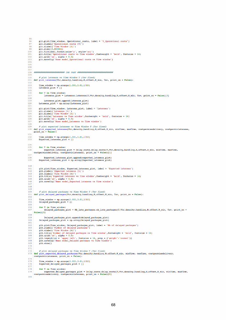
68

69

70
8.1.2 Model 1
Summary
Name file (.py) Inputs Outputs Files used
MODEL 1: TRUCKS + DRONES LAUNCHED FROM DEPOT
11 Geometry_dr T
Vdr
density
handling_dr
R
offset
R_min_dr
Range
payload_avg
payload_max
print_on = False
Float
Float
Float
Float
Float
Float
Float
Float
Float
Float
-
nbrings
summary_geom_dr
table_geom_dr
rings
radius
length
radius_minus
radius_avg
Area
density_rings
w_rings
Float
Matrix
Table
Array
Array
Array
Array
Array
Array
Array
Array
12 Nb_drones T
Vdr
density
handling_dr
R
offset
R_min_dr
Range
payload_avg
payload_max
print_on = False
Float
Float
Float
Float
Float
Float
Float
Float
Float
Float
-
Nk_dr
tot_nb_drones
Array
Float
Geometry_dr_
13 Total_distance_
dr
T
Vdr
density
handling_dr
R
offset
R_min_dr
Range
payload_avg
payload_max
Float
Float
Float
Float
Float
Float
Float
Float
Float
Float
distance_dr
tot_distance_dr
Array
Float
Geometry_dr
Nb_drones
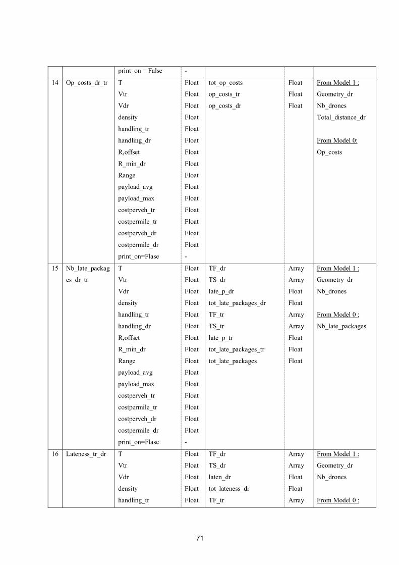
71
print_on = False -
14 Op_costs_dr_tr T
Vtr
Vdr
density
handling_tr
handling_dr
R,offset
R_min_dr
Range
payload_avg
payload_max
costperveh_tr
costpermile_tr
costperveh_dr
costpermile_dr
print_on=Flase
Float
Float
Float
Float
Float
Float
Float
Float
Float
Float
Float
Float
Float
Float
Float
-
tot_op_costs
op_costs_tr
op_costs_dr
Float
Float
Float
From Model 1 :
Geometry_dr
Nb_drones
Total_distance_dr
From Model 0:
Op_costs
15 Nb_late_packag
es_dr_tr
T
Vtr
Vdr
density
handling_tr
handling_dr
R,offset
R_min_dr
Range
payload_avg
payload_max
costperveh_tr
costpermile_tr
costperveh_dr
costpermile_dr
print_on=Flase
Float
Float
Float
Float
Float
Float
Float
Float
Float
Float
Float
Float
Float
Float
Float
-
TF_dr
TS_dr
late_p_dr
tot_late_packages_dr
TF_tr
TS_tr
late_p_tr
tot_late_packages_tr
tot_late_packages
Array
Array
Float
Float
Array
Array
Float
Float
Float
From Model 1 :
Geometry_dr
Nb_drones
From Model 0 :
Nb_late_packages
16 Lateness_tr_dr T
Vtr
Vdr
density
handling_tr
Float
Float
Float
Float
Float
TF_dr
TS_dr
laten_dr
tot_lateness_dr
TF_tr
Array
Array
Float
Float
Array
From Model 1 :
Geometry_dr
Nb_drones
From Model 0 :

72
handling_dr
R,offset
R_min_dr
Range
payload_avg
payload_max
costperveh_tr
costpermile_tr
costperveh_dr
costpermile_dr
print_on=Flase
Float
Float
Float
Float
Float
Float
Float
Float
Float
Float
-
TS_tr
laten_tr
tot_lateness_tr tot_lateness
Array
Float
Float
Float
Lateness
17 Delay_costs
= SUMMARY
of the main
results from (15)
and (16)
T
Vtr
Vdr
density
handling_tr
handling_dr
R,offset
R_min_dr
minTime
maxTime
Range
payload_avg
payload_max
costperveh_tr
costpermile_tr
costperveh_dr
costpermile_dr
costpermissdelivery
costperminlateness
print_on=Flase
Float
Float
Float
Float
Float
Float
Float
Float
Float
Float
Float
Float
Float
Float
Float
Float
Float
Float
Float
-
Total_delayed_packages_
dr
Total_lateness_dr
delay_costs_dr
total_lateness_dr
total_delayed_packages_d
r
Total_delayed_packages_t
r
Total_lateness_tr
delay_costs_tr
total_lateness_tr
total_delayed_packages_tr
Total_delayed_packages
Total_lateness delay_costs
T_av
Float
Float
Array
Array
Array
Float
Float
Array
Array
Array
Float
Float
Array
From Model 1 :
Geometry_dr
Lateness_tr_dr
Nb_late_packages_
dr_tr
From Model 0 :
Delay_costs
18 Main_model_1
= SUMMARY
of the main
results from (1)
to (17)
T
Vtr
Vdr
density
handling_tr
handling_dr
R,offset
Float
Float
Float
Float
Float
Float
Float
tot_op_costs
op_costs_dr
op_costs_tr
tot_nb_drones
tot_distance_dr
tot_nb_trucks
tot_distance
Float
Float
Float
Float
Float
Float
Float
From Model 1 :
Geometry_dr
Nb_drones
Total_distance_dr
Op_costs_dr_tr
Delay_costs_dr_tr
From Model 0 :

73
R_min_dr
minTime
maxTime
Range
payload_avg
payload_max
costperveh_tr
costpermile_tr
costperveh_dr
costpermile_dr
costpermissdelivery
costperminlateness
print_on=Flase
Float
Float
Float
Float
Float
Float
Float
Float
Float
Float
Float
Float
-
delay_costs_dr
delay_costs_tr
delay_costs
Float
Float
Float
Delay_costs
Main_op_costs
10 Plot_model_1
Code
• Geometry_dr.py
74

75
• Nb_drones.py
• Total_distance_dr.py

76
• Operational_costs_dr_tr.py

77
• Nb_late_packages_dr_tr.py

78
• Lateness_tr_dr.py

79
• Delay_costs_tr_dr.py

80

81
• Main_model_1.py
82
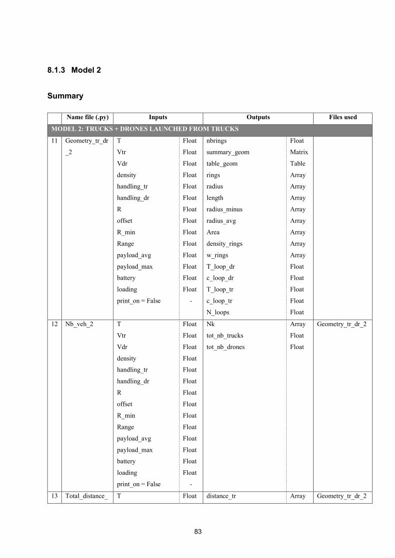
83
8.1.3 Model 2
Summary
Name file (.py) Inputs Outputs Files used
MODEL 2: TRUCKS + DRONES LAUNCHED FROM TRUCKS
11 Geometry_tr_dr
_2
T
Vtr
Vdr
density
handling_tr
handling_dr
R
offset
R_min
Range
payload_avg
payload_max
battery
loading
print_on = False
Float
Float
Float
Float
Float
Float
Float
Float
Float
Float
Float
Float
Float
Float
-
nbrings
summary_geom
table_geom
rings
radius
length
radius_minus
radius_avg
Area
density_rings
w_rings
T_loop_dr
c_loop_dr
T_loop_tr
c_loop_tr
N_loops
Float
Matrix
Table
Array
Array
Array
Array
Array
Array
Array
Array
Float
Float
Float
Float
Float
12 Nb_veh_2 T
Vtr
Vdr
density
handling_tr
handling_dr
R
offset
R_min
Range
payload_avg
payload_max
battery
loading
print_on = False
Float
Float
Float
Float
Float
Float
Float
Float
Float
Float
Float
Float
Float
Float
-
Nk
tot_nb_trucks
tot_nb_drones
Array
Float
Float
Geometry_tr_dr_2
13 Total_distance_ T Float distance_tr Array Geometry_tr_dr_2

84
2 Vtr
Vdr
density
handling_tr
handling_dr
R
offset
R_min
Range
payload_avg
payload_max
battery
loading
print_on = False
Float
Float
Float
Float
Float
Float
Float
Float
Float
Float
Float
Float
Float
-
distance_dr
tot_distance_tr,
tot_distance_dr
Array
Float
Float
Nb_veh_2
14 Op_costs_2 T
Vtr
Vdr
density
handling_tr
handling_dr
R
offset
R_min
Range
payload_avg
payload_max
battery
loading
costperveh_tr
costpermile_tr
costperveh_dr
costpermile_dr
print_on=Flase
Float
Float
Float
Float
Float
Float
Float
Float
Float
Float
Float
Float
Float
Float
Float
Float
Float
Float
-
tot_op_costs
op_costs_tr
op_costs_dr
Float
Float
Float
Nb_veh_2
Total_distance_2
15 Nb_late_packag
es_2
T
Vtr
Vdr
density
handling_tr
Float
Float
Float
Float
Float
TF_dr
TS_dr
late_p_dr
tot_late_packages_dr TF_tr
TS_tr
Array
Array
Float
Float
Array
Geometry_tr_dr_2
Nb_veh_2

85
handling_dr
R
offset
R_min
Range
payload_avg
payload_max
battery
loading
print_on=Flase
Float
Float
Float
Float
Float
Float
Float
Float
Float
-
late_p_tr
tot_late_packages_tr
tot_late_packages
Array
Float
Float
Float
16 Lateness_2 T
Vtr
Vdr
density
handling_tr
handling_dr
R
offset
R_min
Range
payload_avg
payload_max
battery
loading
print_on=Flase
Float
Float
Float
Float
Float
Float
Float
Float
Float
Float
Float
Float
Float
Float
-
TF
TS
laten
tot_lateness
tot_lateness_tr
tot_lateness_dr
Array
Array
Array
Float
Float
Float
Geometry_tr_dr_2
Nb_veh_2
17 Delay_costs_2
= SUMMARY
of the main
results from (15)
and (16)
T
Vtr
Vdr
density
handling_tr
handling_dr
R
offset
R_min
minTime
maxTime
Range
payload_avg
Float
Float
Float
Float
Float
Float
Float
Float
Float
Float
Float
Float
Float
Total_delayed_packages
Total_delayed_packages_tr
Total_delayed_packages_dr
Total_lateness
Total_lateness_tr
Total_lateness_dr
T_av
Float
Float
Float
Float
Float
Float
Array
Lateness_2
Nb_late_packages
_2

86
payload_max
battery
loading
costperveh_tr
costpermile_tr
costperveh_dr
costpermile_dr
costpermissdelivery
costperminlateness
print_on=Flase
Float
Float
Float
Float
Float
Float
Float
Float
Float
-
18 Main_model_2
= SUMMARY
of the main
results from (1)
to (17)
T
Vtr
Vdr
density
handling_tr
handling_dr
R
offset
R_min
minTime
maxTime
Range
payload_avg
payload_max
battery
loading
costperveh_tr
costpermile_tr
costperveh_dr
costpermile_dr
costpermissdelivery
costperminlateness
print_on=Flase
Float
Float
Float
Float
Float
Float
Float
Float
Float
Float
Float
Float
Float
Float
Float
Float
Float
Float
Float
Float
Float
Float
-
tot_op_costs
tot_op_costs_tr
tot_op_costs_dr
tot_op_costs
op_costs_tr
op_costs_dr
summary_all
table_all
nbrings
tot_nb_trucks
tot_nb_drones
tot_distance_tr
tot_distance_dr
Total_delayed_packages
Total_delayed_packages_tr
Total_delayed_packages_dr
Total_lateness
Total_lateness_tr
Total_lateness_dr
delay_costs
delay_costs_tr
delay_costs_dr
T_av
Float
Float
Float
Float
Float
Float
Matrix
Table
Float
Float
Float
Float
Float
Float
Float
Float
Float
Float
Float
Float
Float
Float
Array
Geometry_tr_dr_2
Nb_veh_2
Total_distance_2
Op_costs_2
Delay_costs_2

87
Code
• Geometry_tr_dr_2.py

88
89
• Nb_veh_2.py

90
• Total_distance_2.py
91
• Operational_costs_2.py

92
• Nb_late_packages_2.py

93
• Lateness_2.py
94

95
• Delay_costs_2.py

96
• Main_model_2.py

97