How Much Do Trade Agreements Increase Trade?

A Matching-based Approach

Andrew C. Eggers

January 30, 2006

Abstract

There has been much speculation about whether the recent proliferation of prefer-

ential trade agreements (PTAs) signifies a step toward freer world trade or a retreat

into regionalism. But doubts remain about a prior question, which is whether PTAs

affect trade flows between members at all. In this paper, I address this question using

matching, a technique that reduces the dependence of estimated effects on untestable

modeling assumptions. In contrast to other studies that yield drastically different es-

timates depending on model specification, my approach produces the robust finding

that PTAs increase bilateral trade flows by 15% – 25% five years after creation.

1

1 Introduction

The term “preferential trade agreements” refers to a variety of pacts designed to reduce

trade barriers among signatories. The most limited PTAs are agreements forged between

two nations to lower tariffs on a select group of products. The most expansive PTAs

include a dozen or more countries and involve not just tariff reduction but product-specific

regulatory regimes, programs for reducing non-tariff barriers, and mechanisms for reporting

violations and resolving disputes. The largest and most-well known PTAs include the EU,

NAFTA, and APEC, but as of 2006 there are over 140 in force, including scores of bilateral

agreements. All WTO members except Mongolia are now members of some PTA (Limao,

2005).

Along with the resurgence of PTAs in the 1990s and early 2000s, economists have de-

bated the merits of these agreements. While the value of reducing trade barriers is widely

agreed upon, this particular form of doing so – through preferential and necessarily discrim-

inatory measures – has its drawbacks, both political and economic. From the perspective

of global politics, the development of trade blocs may draw political resources away from

the hard work of global, non-discriminatory liberalization through the WTO. As a matter

of welfare economics, preferential liberalization distorts relative prices and may lead to a

socially costly misallocation of resources.

The challenge of evaluating PTAs has elicited research into both the political dynamics

of international trade negotiations and the theoretical welfare implications of trading blocs.

Both of these research agendas have to some extent relied on the assumption that PTAs

have a significant positive effect on trade flows among their members. But the relatively

boring project of quantifying these effects has encountered surprisingly difficult obstacles.

Estimates vary widely from paper to paper, whether focusing on individual PTAs or all

PTAs, and employ widely different estimation strategies. A recent paper by Ghosh and

2

Yamarik (2004) highlighted these problems, concluding that results depended heavily on

researchers’ prior beliefs and model specifications; another by Magee (2003) concluded that

his estimates varied so widely based on how he specified his trade model that none were

reliable.

While others have pointed out that empirical work has failed to produce robust es-

timates of the effect of PTAs on trade, no one has correctly identified the source of the

problem or proposed a reasonable way to address it. My goal in this paper is to do both. I

argue that the reason why regression-based studies have produced such variable estimates

of the effect of PTAs on trade is that trading partners that form PTAs are not comparable

to most trading partners that don’t. This creates a problem known as “model dependence”:

estimates of the effect of PTAs depend largely on extrapolation, and therefore modeling

assumptions, rather than on the data (King and Zeng, 2006). The solution I implement

here uses matching (Rubin, 2001; Ho et al., 2005) to reduce the dependence of regression

results on the choice of a model. My estimate – that PTAs on average increase trade flows

by between 15% and 25% after five years – is substantively plausible and much more robust

to various model specifications than results obtained using regression alone.

The empirical phenomenon pursued here – the effect of PTAs on trade flows – may not

be intrinsically fascinating, but producing a reliable estimate is useful both to policymakers

and to the ongoing debate about whether regionalism is a stumbling block or stepping-stone

to global free trade. In addition, the methodological challenge of model dependence looms

large in empirical work throughout social science, and the approach I take can be used to

improve estimates of causal effects in countless other areas.

3

2 Preferential trade agreements and their effects: An Overview

PTAs have a long and varied history (see Mansfield and Milner (1999) for more details). A

number of regional customs unions formed in mid-nineteenth century Europe, and, in the

decades between the Anglo-French commercial treaty of 1860 and World War I, the Euro-

pean powers forged dozens of bilateral trade agreements. The interwar period witnessed

Europe’s withdrawal into protectionism, accompanied by fewer, more discriminatory trade

pacts. In the period following World War II, Western European economic integration ad-

vanced under the EEC and European Free Trade Agreement, while Eastern Bloc trade was

structured by the Council for Mutual Economic Assistance (CMEA). Meanwhile, a number

of developing country pacts were established. All of this took place simultaneously with

the development of multilateral economic cooperation under GATT (later WTO), which

was established in part to eliminate the need for preferential arrangements and took a

somewhat dim view of persistent regionalism.

The real upswing in PTA formation occurred with the end of the Cold War. More new

PTAs were registered in the five years from 1990 to 1994 than in any five year period up

to that time (Mansfield and Milner (1999), from WTO figures). Activity since then has

continued to rise and shows no sign of slowing down. In fact, in the twelve months between

January 2004 and February 2005, 43 new agreements were notified to the WTO, 50%

more than in the entire 1990-1994 period and more than in any one-year interval to date.

The new pacts differ from older ones in a number of ways: many of the new agreements

incorporate new states into existing unions (e.g., EU expansion); many link developing and

developed countries, in contrast with earlier pacts, which tended be forged among either

developed or developing countries; and new pacts are more likely to be bilateral than

older ones (Crawford and Fiorentino (2005)). Schiff and Winters (2003) provide a number

of explanations for the uptick in PTA formations. Among the immediate causes, they

4

note PTA signatories’ desire to increase their bargaining power in multilateral negotiations

(Mansfield and Reinhardt, 2003), their interest in strengthening their trading partners

economically and politically, and their desire not to be left behind in the regionalism trend

(a bandwagon effect). More fundamental reasons they cite include the collapse of the Soviet

Union (which resulted in a turn toward capitalism in many states along with an interest

among others in sustaining it), an increasing perception that trade openness is compatible

with and even a cause of economic growth, and the changed attitude of the United States

toward trade blocs, “from active hostility to a broadly enthusiastic stance” (pp. 6–10).

The increasing prevalence of PTAs has not been welcomed by all analysts. Starting

with Jacob Viner’s influential book The Customs Union Issue (1950), economists have

been concerned that the beneficial effects of reducing trade barriers through preferential

trading arrangements might be outweighed by new distortions these arrangements create.

On the one hand, reductions in trade barriers between Country A and Country B can

reduce resource misallocation by making the products of low-cost producers in Country B

available to consumers in Country A, and vice versa. On the other hand, such preferential

arrangements may increase misallocation by making the products of producers in Country

B cheaper for consumers in Country A than those of more efficient producers in non-member

Country C. Viner called the first process “trade-creation” and the second “trade diversion.”

Economists have carried on an extensive debate since Viner about whether preferential

trade agreements have tended to create or divert trade, including both theoretical work

(for an overview, see Panagariya (2000)) and empirical studies (see, e.g., Frankel and

Wei (1998); Eichengreen and Bayoumi (1998)). Depending on whether one thinks these

agreements are trade-creating or trade-diverting, one can view regional trade pacts as

good or bad for economic growth, and therefore as generally constructive stepping stones

to globally free trade or welfare-reducing missteps that should be rectified post haste.

5

While states have pursued PTAs to capture the private benefits of the expected in-

creased trade flows, and economists have theorized about the welfare implications of those

redirected flows, empirical support for the effect of PTAs on trade flows is less solid than

might be expected. A recent paper by Ghosh and Yamarik (2004) argues that, while “a

consensus has emerged among researchers that RTAs are trade creating,” the finding de-

pends heavily on the somewhat ad hoc inclusion or exclusion of particular variables from

the econometric model. Their implication is that researchers in some cases may have cho-

sen regressors to produce a result that confirms their prior belief that PTAs create trade.

Another recent paper (Magee, 2003) finds that PTAs no longer have a robust positive ef-

fect on trade flows when we consider the fact that they are more likely to be formed by

countries that already engage in trade.

Given that so many factors suggest that PTAs should increase trade (most notably, the

fact that all PTAs have the expressed goal of lowering trade barriers), is there any reason to

believe that PTAs do not have the large positive effect on trade that is popularly ascribed

to them? In other words, is there any reason to believe that the small and erratic estimates

of PTA effects in recent papers might reflect reality rather than misguided statistics? Three

main possibilities come to mind. Many PTAs (especially recent ones) have been concluded

largely to cement regional strategic alliances (Schiff and Winters, 2003, chap. 7), and in

these cases trade liberalization may have been less of a priority from the start than would

be assumed from lofty declarations at signing ceremonies. Other PTAs did not implement

the reforms they agreed upon; Frankel and Wei (1998, p. 191) points to ASEAN (the

Association of Southeast Asian Nations), LAFTA (the Latin American Free Trade Area),

and ECOWAS (the Economic Community of West African States) as examples of PTAs

that failed to follow through with liberalization because of delays and a lack of enforcement.

Finally, perhaps preferential liberalization sealed via PTAs has been made irrelevant by

6

the progress of multilateral liberalization; the general decrease in trade barriers may have

swamped selective PTA reductions.

In sum, having a good estimate of the effect of PTAs on trade flows is substantively

important for at least two reasons. First, and most obviously, it could help policymakers

know whether the effort of pursuing PTAs offers a trade payoff. Second, it helps inform

debates about whether PTAs are an obstacle to global free trade. While common sense and

economic theory lead us to believe that trade agreements must spur trade, recent empirical

work has thrown even this belief into question, suggesting that a new approach to the

problem is in order.

3 Model dependence in estimating the effect of PTAs on

trade

The central reason why it is difficult to estimate the effects of trade agreements on trade

flows is that country pairs with trade agreements are so different from country pairs without

them. As a jumping off point, consider the following extremely naive approach to measuring

the effect of PTAs on trade flows: For a given year, calculate the average trade flows between

countries with PTAs. Then, calculate the average trade flows between countries that do

not have PTAs. Subtract the two estimates.

Of course we know that this naive estimate is not a good one, but it is useful to think

about why not. If PTAs were randomly assigned to country-pairs, this naive estimate would

be an unbiased estimator of the effect of PTAs, since the country-pairs with PTAs would

be expected not to differ in any way from the country-pairs without PTAs. If we could

randomly create PTAs (using the language of experiments, “randomly assign the treat-

ment”) to country-pairs, we could be confident that the treatment group (country-pairs

7

with PTAs) would be roughly identical to the control group, not only in the distribution of

important observable characteristics like GDP and distance between the countries, but also

in the distribution of unobservable characteristics like their cultural affinity. If PTAs were

randomly assigned and trade flows differed between treatment country-pairs and control

country-pairs, we could be confident that the difference was due to the existence of the

PTA and not other factors.1

In fact, we know that PTAs are not randomly assigned, and that the treatment and

control group are different in ways that affect their trade flows (and thus render our naive

estimate above a poor estimator of the effect of PTAs). One example is the distance

between the countries. Table 3 reports the distance between countries that signed PTAs

(“Treatment”) and those that did not (“Control”).2 It is well-known that distance between

countries will affect the amount of trading they do, and thus if there are differences in the

distance between countries that sign PTAs and those that do not, the naive estimate above

will be wrong. The Table 3 reports the distance between country pairs at comparable

percentiles within each distribution. Of country pairs that did not sign PTAs, the median

distance is 4,579 miles; the median distance for those that did was less than a third of

that, 1,403 miles. If we try to estimate the effect of PTAs on trade without considering

that PTA-signers are much closer to each other than non-PTA signers, we are likely to

erroneously attribute some of the additional trade that is due to proximity to the existence

of a trade agreement, producing an estimate that is too high.

The traditional response to differences between treatment and control units, in studies

of PTAs as well as most of the rest of social science, has been to use substantive knowledge

to build a model describing the phenomenon we are studying. If the model is good, it1In practice, even in randomized studies the treatment and control group may differ in important ways

requiring regression adjustment.2I introduce the data below.

8

Table 1: Distance between countries (miles)

Treatment Control10th 325 108725th 736 285750th 1403 457975th 3015 692390th 3757 8733

Source: Mansfield and Reiner (2003) dataset, modified as described below.

should tell us what level of trade we should expect between any two pairs of countries with

and without a PTA. In other words, it should tell us what part of the difference in mean

trade flows between PTA- and non-PTA-country pairs is due to the PTA and what part is

due to other differences between PTA and non-PTA pairs.

The standard model of international trade is known as the “gravity model” by analogy

with Newton’s Law of Gravitation; just as the force of gravity between two objects is

increasing in the product of the objects’ masses and the inverse of the square root of the

distance between them, trade flows between two countries are hypothesized to be increasing

in the product of the size of the countries’ economies and decreasing in the distance between

them:

Tij =YiYj

Dij(1)

Econometricians who use the gravity model of trade are quick to point out that, while

it was originally deployed in the 1960’s in an atheoretical manner, the model has since

been justified based on economic theory in a number of different ways. (See Deardorff

(1998) for an example and a discussion.) Still, at its core the model simply says that trade

between two countries should be increasing in the product of their size and decreasing in

the distance between them. All gravity models include some set of additional controls

(such as indicators for whether two countries share a common language, border, or system

9

of government), but no particular economic theory informs the selection of these controls.

Ghosh and Yamarik (2004) argue that this lack of consensus about the details of the

gravity model has produced fragile and unreliable estimates of the effect of PTAs on trade

flows. They identify seventeen covariates that have appeared in at least one (but not most)

of twenty influential gravity models of PTA effects. They divide these “doubtful” variables

into geographic factors (such as remoteness, land area, or common border), historical

factors (such as a common language or colonial history), measures of exchange rate risk,

measures of economic development (such as difference between trading partners’ GDP per

capita), and relative factor endowments. The authors note that the lack of consensus

on which covariates to include in the model suggests that researchers might be selecting

covariates to substantiate prior beliefs about the effect of trade agreements. They conduct

an extreme bounds analysis, showing that the estimated effect of PTAs on trade flows is

highly sensitive to the inclusion or exclusion of the “doubtful” variables erratically employed

in the literature. Including all of the doubtful variables produces the conclusion that 8 of 12

major PTAs created trade, while including none of them3 produces the conclusion that no

PTA they study unambiguously created trade. In short, estimates of the effect of trading

arrangements depend highly on modeling assumptions.

Since I will be returning to this point in the next section, it is important to reemphasize

that the reason we need modeling assumptions, and the reason why the choice of modeling

assumptions affects estimated causal effects, is that important covariates differ between

the treatment and control groups. The modeling assumptions that matter can be divided

into two types: inclusion (which variables to put in the model) and functional form (how

to put them in). It should be clear from the example of distance discussed above that

failing to include a covariate that both differs between control and treatment and affects3This is my reading of the case in which the highest weight is put on their prior, which in every regression

is that the coefficients on doubtful variables have mean zero.

10

the dependent variable will bias estimated treatment effects. Perhaps less obvious is that

the functional form assumption of how a covariate is included in the model affects the

estimated effect if the covariate is correlated with treatment (e.g. if distance is correlated

with PTA membership). If PTAs are formed between nearby countries, and trade declines

with distance exponentially but is included in the model linearly, then the estimated effect

of PTAs may again be biased upwards.

To state the problem in language used more commonly in econometrics, multicollinear-

ity is a problem when the model is misspecified. As is often pointed out in defense of

models with multicollinearity among covariates, multicollinearity in itself does not cause

bias. To be sure, in a study of whether the color of an object affects the force of gravity

acting on it, it matters little whether all of the heavy objects used are red, as long as the

equation for gravity is accurate. The traditional approach in much empirical work has

therefore been to worry about “getting the model right.” In a case like trade, though, it

seems unlikely that any model can ever be “right.” A better approach may be to reduce the

multicollinearity by pruning the dataset. We can make the treatment and control groups

look more similar by eliminating treatment units for which there are no comparable control

units, and eliminating control units for which there are no comparable treatment units.

It may be the practice of throwing out observations that best captures the difference

between traditional regression-based approaches and approaches based on balancing co-

variates. The traditional approach assumes that the structural model is known, and what

is necessary is to gather as much data as possible to estimate the model’s parameters with

maximal precision. If it is a model of trade flows and PTAs, then, it makes little difference

that a particular country-pair without a PTA looks nothing like any country-pair with a

PTA: trade flows between any pair of countries will help estimate the gravity model (which

is assumed to be accurate for all country-pairs), so all pairs should of course be included

11

under this view. The balancing approach takes the view that models are fallible, so it is

better to have a smaller amount of data in which treatment and control groups are more

comparable. When a researcher employing the balancing approach throws out a country-

pair like the US and Vanuatu because it is unlike any country-pair with a PTA, the situation

is perhaps analogous to that when a medical experimenter conducting a study of the effect

of a drug on post-menopause symptoms turns away a five-year old boy volunteering to act

as a control subject.

In the next section, I take this approach as a first step to getting better estimates of

the effect of trade agreements on trade flows.

4 Balancing methods for estimating causal effects

4.1 Defining the treatment

As noted above, the central challenge in estimating causal effects from observational studies

lies in accounting for differences between the treatment and control group that affect the

outcome being studied. Before discussing how balancing methods approach that problem,

it is important to define the treatment.

Studies of the effect of PTAs on trade have typically conducted gravity model-based

regressions that include a binary variable indicating whether a country pair is part of a PTA.

They therefore measure the average difference in trade between countries that have PTAs

and those that do not, controlling for other factors in the gravity model specification they

choose. I choose instead to define treatment as the introduction of a PTA, not the existence

of one. There are two ways to justify this choice. First, how I define treatment affects what

kinds of information I can use in choosing comparable control units. If treatment is defined

as the existence of a PTA, only the standard gravity model covariates (distance, product

12

of GDPs, etc.) can be used. By defining the treatment as the introduction of a PTA, I can

employ data on past trade flows (since both treatment and control units would have no PTA

in the past). It stands to reason that past trade flows would be the best predictors of future

trade flows, and indeed Eichengreen and Irwin (1998) show that even trade numbers from

decades before help improve gravity model predictions of trade flows. By conditioning on

past trade, I am able to address to a large extent concerns raised in Baier and Bergstrand

(2005) about the endogeneity of PTAs. They argue that the standard gravity equation

produces biased estimates of the effect of PTAs because it is missing unobservable variables

(such as the cultural affinity between trading partners) that are correlated with both the

likelihood that two countries will form a PTA and the amount of trade they conduct. Since

I can control for past trade, I can largely eliminate missing variables problems of this kind.

I can also directly address a related problem raised in Magee (2003), which is that the

likelihood of PTA formation depends on past trade volumes. Both Baier and Bergstrand

(2005) and Magee (2003) attempt to address the problems they raise with instrumental

variables techniques, relying upon exclusion restrictions (like the assertion that a country’s

trade does not depend on its form of government) that are highly questionable. By defining

treatment as the initiation of a PTA, I can directly control for past trade and thereby correct

for unobserved determinants of trade in a more reliable way.

A second reason why it makes sense to define treatment as the introduction of a PTA

is that, because trade depends on history (Eichengreen and Irwin, 1998), and because the

terms of PTAs can evolve over time, it seems likely that the effect of a new PTA on trade is

different from the effect of a five-year-old PTA. If that is the case, then defining treatment

as having a PTA rather than forming one, as has been the practice elsewhere, makes it

hard to interpret the resulting estimate of a causal effect. Both for logical clarity and for

practical utility, I want to estimate an effect that corresponds to a policy that could be

13

introduced. If the effect of a PTA depends on its age, then forming a new PTA is a policy

that could be considered; forming a 20-year-old PTA (or, more to the point, a PTA of

average age) is not.

It is important to note that the age of a PTA is not by any means the only source

of variation in PTAs. In fact, arrangements classified as PTAs can address many barriers

to trade or few and make aggressive or incremental reductions in those barriers. Stan-

dard methods in causal inference require that there be only one version of treatment; to

the extent that a PTA is not a single treatment, my estimand becomes, not the average

treatment effect of a PTA, but rather the average effect of the average PTA.4

An additional violation of common causal inference assumptions is that applying treat-

ment to one unit is very likely to affect the outcome for another unit. In this case, forming

a PTA between the US and Mexico is likely to have some effect on trade between the

US and Guatemala, for example, or any other nation to some extent. In contrast to an

ideal laboratory environment, where, for example, administering a drug to one subject is

unlikely to affect the health of another, my estimates of the causal effect of PTAs will thus

be imperfectly estimated. For example, if forming a PTA with country A diminishes trade

with country B, then our estimate of the effect of forming a PTA with country A will be

too large, given that trade with country B is being used to create a counterfactual level of

trade with country A.

It should be noted, though, that while these complications (both of which constitute

violations of SUTVA (Stable Unit Treatment Value Assumption) (Imbens and Rubin, 2006,

Chapter 1)) make this setting imperfect for estimating causal effects, the same problems

occur in every observational study of PTAs yet conducted. The main contribution of this4In the ideal setting, such as laboratory experiment, the treatment is made as uniform as possible. The

reason for using many units of observation (and the justification for seeking out an “average treatmenteffect”) is that the response of the units to the treatment may differ due to unobserved differences betweenthe units. The “average” in “average treatment effect” thus modifies “effect,” not “treatment.”

14

paper is to produce estimates that depend less on modeling assumptions than those other

studies, and in that sense the causal inference techniques I employ are an improvement on

previous techniques with little cost.

4.2 Considerations in balancing these data

The goal of balancing is to make treatment and control groups as similar as possible, like

treatment and control groups in a randomized study. But this general goal leaves significant

leeway for different practices. The ideal would be to find an exact match for each treated

unit – for example, a pair of countries that is exactly the same as the US and Mexico in

1994 in every way but did not form a PTA. In practice, of course, this is not possible, and

we must make tradeoffs of two kinds. One kind of tradeoff is among covariates: should we

prioritize finding pairs of countries with similarly sized economies, or with similar distances

between them? Another tradeoff is about similarity in general: how different can country

pairs be before we decide to discard the treated unit entirely (if, for example, no control

pair is similar enough to the US and Canada when they enacted their trade pact in 1989)?

Methodologists have not yet come to a consensus on the answers to these questions. To

some extent, opinions differ based on one’s position on parametric modeling. To some

analysts, such as Ho et al. (2005), the goal of balancing is to reduce model dependence

– to improve the reliability of estimates made in parametric models. To others, the goal

of balancing is to replace parametric modeling, and produce non-parametric estimates of

the treatment effect such as the difference in mean trade flows between the treatment and

control groups. Those who take the latter view accept less imbalance and seek out more

elaborate means of eliminating it. Here, I pursue an approach more in the spirit of Ho

et al. (2005).

Accordingly, my goal in balancing is to reduce as much as possible the difference between

15

treatment and control units in the covariates that we would normally include in a model

of trade. The core variables in gravity models are distance between trading partners and

the log product of their GDPs, but I consider several other variables often employed: the

difference in their GDP per capita, and indicators for whether they are adjacent, whether

they are both democracies, whether they are part of a security alliance, and whether they

have a former colonial relationship. I believe it is also important to balance on the year,

since trade flows have shown a secular rise over time with rising incomes and decreasing

transport costs. More important than these variables, for reasons I outlined above, is past

trade flows.

My approach in matching was as follows.5 I first restricted the donor pool such that

a dyad-year (a pair of countries in a particular year) can be chosen as a match only for

a treatment unit of the same year. (In other words, I matched exactly on year.) I next

prioritized matching on trade flows two and four years before the enactment of the PTA.

I chose not to match on trade flows in the year of the PTA formation or the previous

year, since it is widely recognized that trade could surge in anticipation of the PTA. While

there is likely some anticipation even two years before enactment, it seemed a reasonable

compromise to start the matching there. Finally, I matched on a propensity score calculated

on the remaining gravity model variables – the fitted values of a linear probability model

predicting treatment based on distance and the indicators I listed above. As is typical of

dyadic studies, the data included a large donor pool of control units to choose from – in the

final dataset we have 284 treatment dyad-years and over 40000 control dyad-years. The

large number of control units helps ensure that we will get fairly good matches. It also

means that we can choose more than one control unit for each treatment unit; compared to

choosing only one control unit, choosing more matches tends to increase bias (since the first5I used the “Matching” package written for R by Jasjeet Sekhon and available publicly at the CRAN

archive.

16

one was the best) but decrease the variance of the estimated treatment effect (Imbens and

Rubin, 2006, Chapter 6:17). I decided to choose three matches for each treated unit. I then

experimented with a number of different ways of prioritize balancing the previous trade

variables and the propensity score (i.e. different weights in a Mahalanobis matrix) before

choosing a matched dataset that balanced previous trade sufficiently while not leaving too

much bias in the other covariates.

4.3 The data

Before reviewing the covariate balance before and after matching, I will briefly introduce

the data. I use a dataset assembled by Edward D. Mansfield and Eric Reinhardt for their

paper on the relationship between the WTO and the formation of PTAs (Mansfield and

Reinhardt, 2003) and made available on Reinhardt’s website.6 Mansfield and Reinhardt

include only reciprocal PTAs (agreements that involve reciprocal reductions in trade bar-

riers) registered with the WTO; this definition excludes agreements such as the Caribbean

Basin Economic Recovery Act, in which the US unilaterally reduced tariffs for Caribbean

countries.

The dataset includes bilateral trade flows between 137 countries over the period from

1948 to 1998, for a potential number of 475,116 dyad-year observations.7 In fact, only

18 countries (and thus 153 unique dyads) have trade data over the whole period, with

the average number of years per dyad just over 30 years. Further, much of the data on

political and economic factors that enter into my subsequent analysis is missing for many

observations in the dataset, such that many observations must be deleted before analysis.8

6http://userwww.service.emory.edu/ erein/7To arrive at the figure 475,116, note that there are 137 countries in the dataset, each of which has 136

pairs, producing a total of 18,632 dyads; since each pair has a mirror image, divide by 2; and multiply by51 for the number of years in the period 1948-1998.

8In future extensions of this work I will use multiple imputation to take advantage of all the data. SeeKing et al. (2001).

17

As noted above, I define treatment as the formation of a PTA; as control observations I

include dyad-years in which there is no PTA and none will be formed for the next 5 years.

(I thus delete all observations with existing PTAs and any in which a PTA will be formed

within 5 years.) Following all these omissions, the dataset consists of 40,438 observations,

each of which represents a dyad of countries in a particular year between 1948 and 1998.

Of these, 284 are treatments – new PTAs formed.

4.4 Matching and assessing balance

As mentioned above, the matching algorithm tries to find three control dyads for each

treated dyad. In some cases, the algorithm failed to find good enough matches and settled

for one or two matches instead. For example, the United States and Canada formed

the NAFTA forerunner in 1989; the algorithm chose the US and Japan (in 1989) as a

comparable match, no doubt prioritizing the level of bilateral trade, but declined all other

matches based on a tolerance setting. Out of 852 potential matches (= 284 × 3) the

algorithm produced 849.

To what extent has the matching algorithm succeeded in making the control group more

like the treated group? To give a preliminary sense, Appendix A lists 20 matches, chosen

at random from the 1096 total matches. The left column indicates a treatment pair (a

dyad-year in which a PTA was formed) and the right column lists one of its corresponding

matches. Looking at the matches, it is clear that the pairs differ in many ways (distance

between the countries, form of government, climate). The important thing, not always

apparent from superficial knowledge of the countries, is that these pairs of dyads engaged

in a similar amount of trade in the years before the year in which the treatment dyad

formed a PTA. For example, the first match (Italy-Denmark and Canada-France, both in

1970) conducted $697 million and $727 million in trade in 1968, respectively, and $618

18

million and $695 million in trade in 1966.

Figures 1 to 3 provide a more systematic view of the improvement in balance achieved

by the matching process. Each figure depicts density and quantile plots for the matched and

unmatched datasets on a covariate important in predicting trade. The top left panel depicts

the density (essentially, a smoothed histogram) for the treatment (solid line) and control

groups (dashed line) in the unmatched dataset.The top right panel depicts a quantile plot:

a single dot plots the value in the control group (x-axis) against the value in the treatment

(y-axis) of equal percentile observations, e.g. it plots the 50th percentile trade flows in

the control group (x-axis) against the 50th percentile trade flows in the treatment group

(y-axis). The bottom panels do the same for the matched dataset.

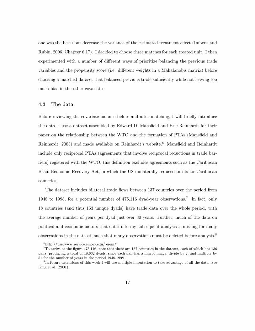
For example, Figure 1 assesses balance for the logarithm of trade flows (in trillions

of dollars) two years before the signing of a PTA. The unmatched control group here

consists of all dyad-years with no current PTA and none formed in the next five years.

The top left panel shows that trade flows are distributed somewhat lower for non-signers

(the dashed line); the top right panel confirms this, showing that, for a given percentile

of trade flows, the treatment group (y-axis) has more trade than the control group. After

matching, though, this discrepancy has been largely erased. The density plots (bottom

left) are almost identical, and the quantile plot (bottom right) lies neatly on the 45 degree

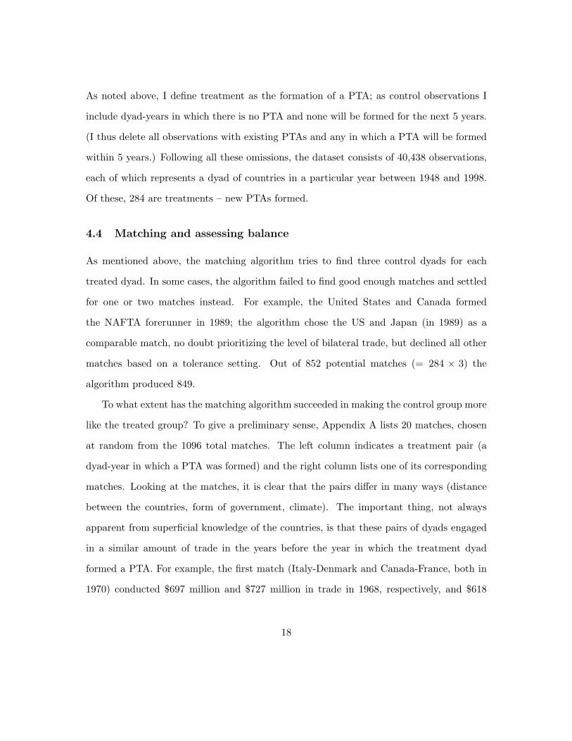
line. Figure 2 shows a similar degree of improvement in the balance for trade four years

before PTA formation.

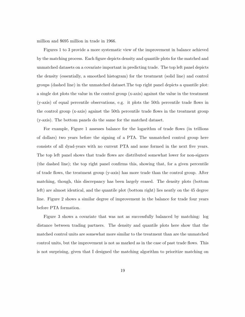
Figure 3 shows a covariate that was not as successfully balanced by matching: log

distance between trading partners. The density and quantile plots here show that the

matched control units are somewhat more similar to the treatment than are the unmatched

control units, but the improvement is not as marked as in the case of past trade flows. This

is not surprising, given that I designed the matching algorithm to prioritize matching on

19

Figure 1: Log trade flows two years before PTA formation – Density and quantileplots for unmatched and matched datasets

−15 −10 −5

0.00

0.05

0.10

0.15

0.20

Unmatched

Log trade flows

●

●●●●●●●●●●●●●●●

●●●●●●●●●●●●●●●●●●●●●●●●●●●●●●●●●●●●●●

●●●●●●●●●●●●●●●●●●●●●●●●●●●●●●●●●●●●●●●●●●●●●●●●●●●●●●●●●●●●●●●●●●●●●●●●●

●●●●●●●●●●●●●●●●●●●●●●●●●●●●●●●●●●●●●●●●●●●●●●

●●●●●●●●●●●●●●●●●●●●●●●●●●●●●●●●●●●●●●●●●●●●●●●●●●●●●

●●●●●●●●●●●●●●●●●●●●●●●●●●●●●●

●●●●●●●●●●●●●●●●●●●●●●●●●

●●

●

−15 −10 −5

−15

−10

−5

Unmatched

Control

Tre

atm

ent

−15 −10 −5

0.00

0.05

0.10

0.15

0.20

Matched

●

●●●●●●●●●●

●●●●●●●●●●●●●●●●●●●

●●●●●●●●●●●●●●●●●●●●●●●●

●●●●●●●●●●●●●●●●●●●●●●●●●●●●

●●●●●●●●●●●●●●●●●●●●●●●●●●●●●●●●●●●●●●●●●●●●●

●●●●●●●●●●●●●●●●●●●●●●●●●●●●●●●●●●●●●●●●●●●●●●●●●●●●●●●●●●●●●●●●●●●●●●●●●●●●●●●●●●●●●●●●●●●●●●●●●●●●●●●●●●●●●●●●●●●●

●●●●●●●●●●●●●●●●●●●●●●●●●●●●●●●●●●●●●●

●●

●

−15 −10 −5

−15

−10

−5

Matched

Tre

atm

ent

The solid line in the top left panel depicts the density (smoothed histogram) of trade flowstwo years before PTA formation; the dashed line shows the density for all dyad-years thatdid not form a PTA. Since the control density is to the left of the treatment density, weknow that PTA signers generally had higher trade two years before signing than didcountries that did not sign a PTA. The same conclusion can be drawn from the quantileplot on the top right. The top right panel shows that, for a given percentile of trade flows,the treatment group (y-axis) has more trade than the control group (x-axis). Aftermatching, though, this discrepancy has been largely erased. The matching algorithmproduced a control set with a distribution of lagged trade very similar to that of thetreatment group.

20

Figure 2: Log trade flows four years before PTA formation – Density and quantileplots for unmatched and matched datasets

−14 −12 −10 −8 −6 −4 −2

0.00

0.05

0.10

0.15

0.20

Unmatched

Log trade flows

● ●●●●●

●●●●●●●●●

●●●●●●●●●●●●●●●●●●●●

●●●●●●●●●●●●●●●●●●●●●●●●●●●●

●●●●●●●●●●●●●●●●●●●●●●●●●●●●●●●●●●●●●●●●●●●●●●●●●●●●●●●●●●●●●●

●●●●●●●●●●●●●●●●●●●●●●●●●●●●●●●●●●●●●●●●●●●●●

●●●●●●●●●●●●●●●●●●●●●●●●●●●●●●●●●●●●●●●●●●●●●●●●

●●●●●●●●●●●●●●●●●●●●●●●●●●●●●●●●

●●●●●●●●●●●●●●●●●●●●●●●●●●●

●●●●●●

●

−14 −12 −10 −8 −6 −4 −2

−14

−10

−8

−6

−4

−2

Unmatched

Control

Tre

atm

ent

−14 −12 −10 −8 −6 −4 −2

0.00

0.05

0.10

0.15

0.20

Matched

●●●●●●●●●●

●●●●●●●●●●

●●●●●●●●●●●●●●●

●●●●●●●●●●●●●●●●●●●●●●●●●●●●

●●●●●●●●●●●●●●●●●●●●●●●●●●●●●●●●●●●●●●●

●●●●●●●●●●●●●●●●●●●●●●●●●●●●●●●●●●●●●●●●●●●●●●●●●●●●●●●●●●●●●●●●●●●●

●●●●●●●●●●●●●●●●●●●●●●●●●●●●●●●●●●●●●●●●●●●●●●●●

●●●●●●●●●●●●●●●●●●●●●●●●●●●●●●●●

●●●●●●●●●●●●●●●●●●●●●●●●●●●

●●●●●●

●

−14 −12 −10 −8 −6 −4 −2

−14

−10

−8

−6

−4

−2

Matched

Tre

atm

ent

Matching produced a control set with a distribution of lagged trade very similar to that of the treatmentgroup. See Figure 1 for more interpretation.

21

Figure 3: Log distance (in thousands of miles) between countries in the dyad –Density and quantile plots for unmatched and matched datasets

−1 0 1 2

0.0

0.2

0.4

0.6

0.8 Unmatched

Distance

●●●●●●● ● ● ●●●●●●●●●●●●●●●●●●●●●●●●●●●●●●●●●●●●●●●●●●●●●●●●●●●●●●●

●●●●●●●●●●●●●●●●●●●●●●●●●●●●●●●●●●●●●●●●●●●●●●●●●●●●●●●●●●●●●●●●●●●●●●●●●●●●●●●●●●●●●●●●●●●●●●●●●●●●●●●●●●●●●●●●●●●●●●●●●●●●●●●●●●●●●●●●●●●●●●●●●●●●●●●●●●●●●●●●●●●●●●●●●●●●●●●●●●●●●●●●●●●●●●●●●●●●●●●●

●●●●●●●●●●●●●●●●●●●●

−1 0 1 2

−1

01

2

Unmatched

ControlT

reat

men

t

−1 0 1 2

0.0

0.2

0.4

0.6

0.8 Matched

●●●●●●●●●●●●●●●●●●●●●●●● ●●●●●●●●●●●●●●●●●●●●●●●●●●●●●●●●●●●●●●●●

●●●●●●●●●●●●●●●●●●●●●●●●●●●●●●●●●●●

●●●●●●●●●●●●●●●●●●●●●●●●●●●●●●●●●●●●●

●●●●●●●●●●●●●●●●●●●●●●●●●●●●●●●●●●●●●●●●●●●●●●●●●●●●●●●●●●●●●●●●●●●●●●●●●●●●●●●●●●●●●●●●●●●●●●●●●●●●●●●●●●●●●●●●●●●●●●●●●●●●●●●●●●●●●●●●●●●●●●●●●

●●●

−1 0 1 2

−1

01

2

Matched

Tre

atm

ent

Because of its lower priority in the matching algorithm, there was less improvement in balance on logdistance. See Figure 1 for more interpretation.

past trade; distance and other covariates can be thought of as tiebreakers among control

dyads with trade histories equally similar to a given treated unit. In fact, it’s likely that

much of the improvement in balance in distance comes from choosing control dyads with

more similar past trade flows.

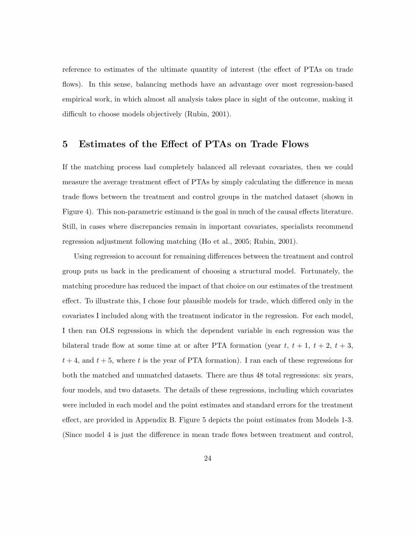
A final measure of balance is provided in Figure 4. The figure plots the mean log trade

(in trillions of $US) by year, where year 0 is the year of PTA formation, for the matched

dataset. It is not surprising that mean trade flows for treatment and control are very close

for t − 2 and t − 4, since we matched on those values. It is reassuring, though, that the

balance also looks good for t− 5 and t− 3, which I could have matched on as well. What’s

more, the values are quite close for t − 1 and t. (The lowest p-value on a two-sided test

22

Figure 4: Mean log trade in matched treatment and control groups

●

●

●●

●

●

●

●

●

●

●

−4 −2 0 2 4

−9.

0−

8.8

−8.

6−

8.4

−8.

2

Year

Ave

rage

trad

e in

log

trill

ions

of d

olla

rs

Treatment

Control

Mean log trade before the treatment is applied is roughly equal for the treated and control groups aftermatching. This suggests that matching was successful in reducing model dependence. The gap that opensup after year 0 is an indication that PTAs increase trade by roughly 20% after the third year in force,although discrepancies remaining between treatment and control groups call for regression adjustment.

for the equality of means for any of these lags is .81.) It appears that there are fewer

anticipatory effects than I suspected, since PTAs do not seem to substantially affect trade

until they go into effect. 9

It appears from Figure 4 that a gap between the treated and control units opens up in

the years following enactment of the PTA. This gap could be interpreted as an initial, non-

parametric estimate of the average causal effect of PTAs. It is important to note, however,

that all of the balancing exercises up to this point could be (and were) carried out without9Testing for the equality of mean trade flows before the PTA goes into effect is one type of test for

unconfoundedness – the property that, conditional on observed covariates, units were assigned to treatmentindependent of outcomes. In other words, while treatment was not randomly assigned, we can say treatmentwas unconfounded if we observe the covariates on which treatment was assigned, and, controlling for thosecovariates, treatment was not assigned based on whether trade would be high or low. While we cannot provethat the matched dataset is unconfounded in this sense, we could be confident that it was not unconfoundedif lagged trade figures differed between treated and control groups. The matched dataset passes this test.

23

reference to estimates of the ultimate quantity of interest (the effect of PTAs on trade

flows). In this sense, balancing methods have an advantage over most regression-based

empirical work, in which almost all analysis takes place in sight of the outcome, making it

difficult to choose models objectively (Rubin, 2001).

5 Estimates of the Effect of PTAs on Trade Flows

If the matching process had completely balanced all relevant covariates, then we could

measure the average treatment effect of PTAs by simply calculating the difference in mean

trade flows between the treatment and control groups in the matched dataset (shown in

Figure 4). This non-parametric estimand is the goal in much of the causal effects literature.

Still, in cases where discrepancies remain in important covariates, specialists recommend

regression adjustment following matching (Ho et al., 2005; Rubin, 2001).

Using regression to account for remaining differences between the treatment and control

group puts us back in the predicament of choosing a structural model. Fortunately, the

matching procedure has reduced the impact of that choice on our estimates of the treatment

effect. To illustrate this, I chose four plausible models for trade, which differed only in the

covariates I included along with the treatment indicator in the regression. For each model,

I then ran OLS regressions in which the dependent variable in each regression was the

bilateral trade flow at some time at or after PTA formation (year t, t + 1, t + 2, t + 3,

t + 4, and t + 5, where t is the year of PTA formation). I ran each of these regressions for

both the matched and unmatched datasets. There are thus 48 total regressions: six years,

four models, and two datasets. The details of these regressions, including which covariates

were included in each model and the point estimates and standard errors for the treatment

effect, are provided in Appendix B. Figure 5 depicts the point estimates from Models 1-3.

(Since model 4 is just the difference in mean trade flows between treatment and control,

24

the estimated effect of treatment (a 500% increase in trade) isn’t really plausible for the

unmatched dataset.) Each model predicts that forming a PTA increases bilateral trade, and

that the increase grows somewhat over the years following formation. For the unmatched

dataset, the estimated impact of PTAs varies widely across models: the predicted impact

of forming a PTA on trade five years later varies from 25% to about 75%. The estimated

effect forming a PTA depends far less on the choice of a model for the matched dataset:

the range of estimates for the impact on trade at t + 5 is 15% (Model 2) to 26% (Model

3). For comparison, I also plot the nonparametric estimate produced using Model 4 for the

matched dataset. While this estimate is off the chart for the unmatched dataset, the result

using the matched dataset is not markedly different from parametric estimates from the

other models. The estimated treatment effect here depends on the data and the matching

algorithm chosen, but it depends very little on the choice of a parametric model for trade.

To give an idea of the degree of precision associated with the point estimates in Figure 5,

I chose one model (Model 2) and used a simulation approach to show the range of estimated

causal effects. Using the regression output from Model 2 applied to the matched sample,

I produced 1000 simulated counterfactuals for each of the treated units (i.e., trade flows

under the assumption that they had not created at PTA) for (t, t + 1, ..., t + 5). For each

simulation, I calculated the mean difference between the observed values and the imputed

counterfactual values – an estimate of the average treatment effect for the treated (ATT)–

and converted the result into a percentage increase in trade compared to the counterfactual

estimate. In Figure 6, I then plotted the density of these estimates for each year following

signing of the PTA. Because the treatment is not interacted with anything in the model,

the resulting density is similar to a normal density centered on the point estimate, with the

standard deviation equal to the standard error from the regression. The figure reinforces

the impression that the effect of signing a PTA rises over the first several years; after three

25

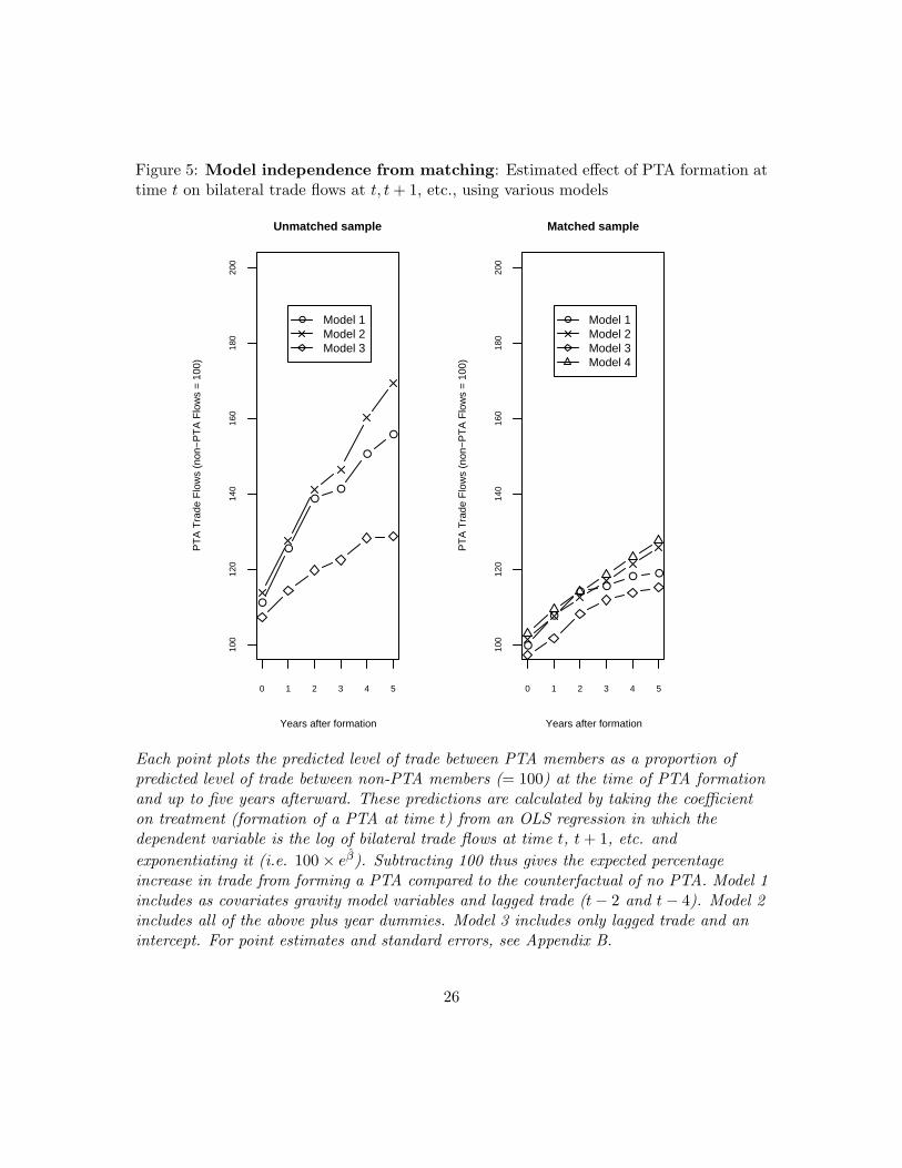
Figure 5: Model independence from matching: Estimated effect of PTA formation attime t on bilateral trade flows at t, t + 1, etc., using various models

0 1 2 3 4 5

100

120

140

160

180

200

Unmatched sample

Years after formation

PT

A T

rade

Flo

ws

(non

−P

TA

Flo

ws

= 1

00)

●

●

●●

●

●

● Model 1Model 2Model 3

0 1 2 3 4 5

100

120

140

160

180

200

Matched sample

Years after formation

PT

A T

rade

Flo

ws

(non

−P

TA

Flo

ws

= 1

00)

●

●

●●

● ●

● Model 1Model 2Model 3Model 4

Each point plots the predicted level of trade between PTA members as a proportion ofpredicted level of trade between non-PTA members (= 100) at the time of PTA formationand up to five years afterward. These predictions are calculated by taking the coefficienton treatment (formation of a PTA at time t) from an OLS regression in which thedependent variable is the log of bilateral trade flows at time t, t + 1, etc. andexponentiating it (i.e. 100× eβ̂). Subtracting 100 thus gives the expected percentageincrease in trade from forming a PTA compared to the counterfactual of no PTA. Model 1includes as covariates gravity model variables and lagged trade (t− 2 and t− 4). Model 2includes all of the above plus year dummies. Model 3 includes only lagged trade and anintercept. For point estimates and standard errors, see Appendix B.

26

years, having a PTA increases trade flows by about 15%.

This estimate of the effect of PTAs is extremely blunt, treating all 284 PTAs in my

data as equivalent. It would be useful to categorize PTAs by type and evaluate their

effects separately in order to produce finer-grained observations the effect they have had.

For example, we could ask whether PTAs have become more or less effective over time; we

could ask whether features of a country pair (such as whether they are both industrialized

or combine a rich and a poor country) makes a PTA create more or less trade. Schiff and

Winters (2003) emphasize that, because a rich country can enforce club rules on developing

country trading partners through a PTA, “North-South” PTAs should produce more policy

reform and thus more investment and trade than other types of PTAs.

In theory, this should be an easy exercise using these methods. It should be possible

to take the matched dataset, strip out the subset of treatment pairs we are interested in

along with their associated matches, conduct whatever regression adjustment is necessary

within this subset of the data, and produce counterfactual estimates of trade for the subset

of treated units. In my attempts to do this and produce more informative estimates of the

effect of PTAs on trade, I found that the matching procedure worked less well for subsets

of the data than for the whole dataset. In particular, treatment was no longer plausibly

unconfounded: for some subsets of the matched dataset, treated pairs engaged in consid-

erably more or considerably less trade than control pairs even well before creation of the

PTA. As a result, parametric estimates of the treatment effect once again depended highly

on the functional form. This problem should be to some extent expected for matching

with small datasets, but the lack of balance is surprising given that some of the subsets I

was looking at had around 150 treated pairs. I suspect there is something wrong with the

procedure I am using but decided to write up my results rather than pursue this further.

I will address the issue in future version of this paper.

27

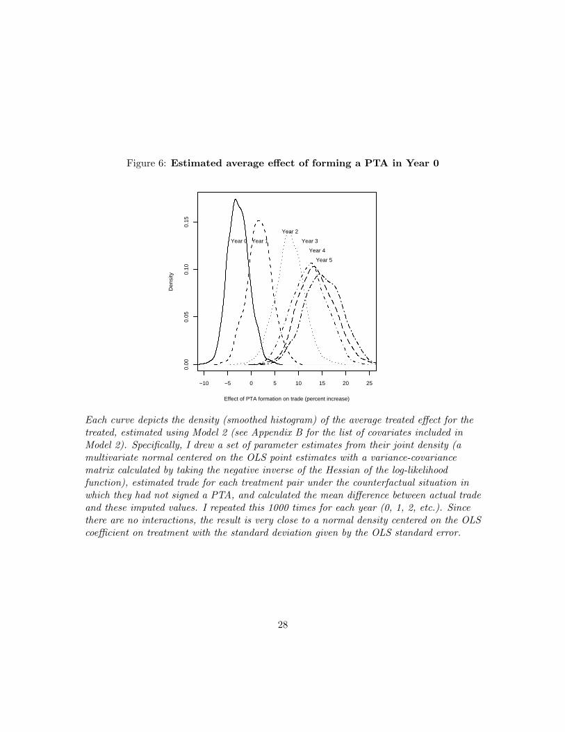
Figure 6: Estimated average effect of forming a PTA in Year 0

−10 −5 0 5 10 15 20 25

0.00

0.05

0.10

0.15

Effect of PTA formation on trade (percent increase)

Den

sity

Year 0 Year 1

Year 2

Year 3

Year 4

Year 5

Each curve depicts the density (smoothed histogram) of the average treated effect for thetreated, estimated using Model 2 (see Appendix B for the list of covariates included inModel 2). Specifically, I drew a set of parameter estimates from their joint density (amultivariate normal centered on the OLS point estimates with a variance-covariancematrix calculated by taking the negative inverse of the Hessian of the log-likelihoodfunction), estimated trade for each treatment pair under the counterfactual situation inwhich they had not signed a PTA, and calculated the mean difference between actual tradeand these imputed values. I repeated this 1000 times for each year (0, 1, 2, etc.). Sincethere are no interactions, the result is very close to a normal density centered on the OLScoefficient on treatment with the standard deviation given by the OLS standard error.

28

6 A remaining source of bias?

By matching (selecting a control set of country-pairs with similar characteristics to country-

pairs that formed PTAs), I have produced estimates of the effect of PTAs that rely far less

on untestable modeling assumptions than previous research. Still, the results depend on

what covariates I choose to match on.

One covariate that I did not control for is the degree to which members of a country

pair intend to liberalize their trade policies. I have followed standard practice in viewing

a PTA as a set of policies for preferential liberalization that are not being carried out by

non-PTA signatories. (In other words, I have assumed that PTA members engage in a

kind of preferential liberalization that non-PTA members do not.) This assumption may

be justified in two ways: first, the WTO does not permit preferential trade outside of

the auspices of a notified PTA; second, states may not find it possible to substantially

liberalize without the formal, public, and reciprocal structure of a PTA. (See Appendix

C for an extended consideration of these issues.) But bilateral trade flows may also be

affected by non-preferential liberalization, such as a general reduction in tariffs. If there is

a correlation between PTA formation and non-preferential liberalization, then my estimates

of the effect of PTAs may be biased. For example, if PTA signatories are more likely to

liberalize generally, then trade flows of PTA signatories may grow more quickly than those

of non-PTA signatories because of their general liberalization policies rather than their

PTAs.

The task then is to identify countries that are lowering their trade barriers and account

for this by matching and/or regression. It would probably be necessary to consider only

policies enacted before the PTA was concluded, since policies enacted after might have been

affected by the PTA, and thus should technically be considered part of the treatment effect.

(Perhaps more to the point, many measures of trade policy orientation (such as the ratio

29

of tariff revenue to trade volume) would be affected by the PTA.) There are many existing

measures of trade policy openness, although economists disagree about how informative

they are (see, e.g., Rodrguez and Rodrik (2001) and Edwards (1998)). Ideally, matching

country-pairs with similar trade policy profiles would eliminate this potential source of bias

in my estimates of the effect of PTAs on trade volumes. This exercise remains for future

research.

7 Conclusion

The aim of this paper was to improve on existing estimates of the effect of preferential

trade agreement on trade. Previous work relied on the gravity model to estimate how

much extra trade PTA members engaged in. This is asking a lot of a simple model, since

PTA signatories are very different from non-signatories in ways that heavily affect trade.

The result has been that estimates of the effect of PTAs vary widely according to the

specification employed.

My approach improves on earlier work in two main ways. First, by defining the “treat-

ment” as the initiation of a PTA, I make it possible to control for past trade flows, which

makes predictions of counterfactual trade more precise. Second, I use a matching procedure

to select a control group that is similar to the treatment group in ways that affect trade.

As a result of these two choices, my estimates of the effect of PTAs on trade are fairly

stable even when radically different regression models are used. When the same battery of

models is applied to unmatched data, estimates vary widely, as is typical of other results

in this literature.

Examining PTAs initiated between the 1950s and the early 1990s, I find that signing

a preferential trade agreement increased bilateral trade five years later by between 15%

and 20%. In future extensions of this project, I hope to account for a possible remaining

30

source of bias (changes in overall trade policy that are correlated with PTA adoption), and

I plan to produce estimates of the effect of PTAs that give an idea of how that effect has

changed over time and how it depends on the particular PTA or characteristics of country-

pairs. As it stands, though, this paper applies a new technique that provides a plausible

and comparatively robust answer to a troubling empirical puzzle in the international trade

literature.

31

References

Baier, S. L. and Bergstrand, J. H. (2005). Do free trade agreements actually increase

members’ international trade? Federal Reserve Bank of Atlanta Working Paper Series,

2005-3.

Crawford, J.-A. and Fiorentino, R. V. (2005). The changing landscape of regional trade

agreements. WTO Discussion Paper, No. 8.

Davis, C. (2004). International institutions and issue linkage: Building support for agri-

cultural trade liberalization. American Political Science Review, 98(1):153–169.

Deardorff, A. V. (1998). Determinants of bilateral trade: does gravity work in a classical

world?, pages 7–22. University of Chicago Press, Chicago.

Edward D. Mansfield, H. V. M. and Rosendorff, B. (2002). Why democracies cooperate

more: Electoral control and international trade agreements. International Organization,

56(3):477–513.

Edwards, S. (1998). Openness, productivity, and growth: What do we know? The Eco-

nomic Journal, 108(447):383–398.

Eichengreen, B. and Bayoumi, T. (1998). Is Regionalism Simply a Diversion? Evidence

from the EU and EFTA. University of Chicago Press, Chicago.

Eichengreen, B. and Irwin, D. A. (1998). The Role of History in Bilateral Trade Flows,

pages 33–57. University of Chicago Press, Chicago.

Fernandez, R. and Portes, J. (1998). Returns to regionalism: An analysis of nontraditional

gains from regional trade agreements. World Bank Economic Review, 12(2):197–220.

32

Frankel, J. A. and Wei, S.-J. (1998). Regionalization of World Trade and Currencies:

Economics and Politics, pages 189–226. University of Chicago Press, Chicago.

Ghosh, S. and Yamarik, S. (2004). Are regional trading arrangements trade creating? an

application of extreme bounds analysis. Journal of International Economics, 64:369–395.

Ho, D. E., Imai, K., King, G., and Stuart, E. (December 4, 2005). Matching as nonpara-

metric preprocessing for reducing model dependence in parametric causal inference.

Imbens, G. and Rubin, D. (2006). Causal inference. Unpublished textbook manuscript.

King, G., Honaker, J., Joseph, A., and Scheve, K. (2001). Analyzing incomplete political

science data: An alternative algorithm for multiple imputation. American Political

Science Review, 95(1):49–69.

King, G. and Zeng, L. (2006). When can history be our guide? the pitfalls of counterfactual

inference. Forthcoming in International Studies Quarterly.

Limao, N. (August, 2005). The clash of liberalizations: Preferential trade agreements as a

stumbling block to multilateral liberalization. Comments prepared for the conference in

honor of Jagdish Bhagwatis 70th birthday at Columbia University, August 5th and 6th

2005.

Magee, C. S. (2003). Endogenous preferential trade agreements: An empirical analysis.

Contributions to Economics Analysis and Policy, 2:1–17.

Mansfield, E. D. and Milner, H. V. (1999). The new wave of regionalism. International

Organization, 53:589–627.

Mansfield, E. D. and Reinhardt, E. (2003). Multilateral determinants of regionalism. In-

ternational Organization, 57:829–862.

33

Panagariya, A. (2000). Preferential trade libealization: The traditional theory and new

developments. Journal of Economic Literature, 38:287–331.

Rodrguez, F. and Rodrik, D. (2001). Trade Policy and Economic Growth: A Skeptic’s

Guide to the Cross-National Evidence. MIT Press, Cambridge, MA.

Rubin, D. (2001). Using propensity scores to help design observational studies: Application

to the tobacco litigation. Health Services and Outcomes Research Methodology, 2:169–

188.

Schiff, M. and Winters, L. A. (2003). Regional Integration and Development. The World

Bank, Washington, D.C.

Simmons, B. A. and Hopkins, D. J. (2005). The constraining power of international treaties:

Theory and methods. American Political Science Review, 99(4):623–631.

34

Appendix A: A sample of matches

Treatment Matched control

[1,] "Italy Denmark 1970" "Canada France 1970"

[2,] "Portugal Italy 1973" "Chile Italy 1973"

[3,] "Germany Cyprus 1973" "Switzerland Turkey 1973"

[4,] "Luxembourg Turkey 1964" "Czechoslovakia Sweden 1964"

[5,] "Switzerland Spain 1980" "France Yugoslavia 1980"

[6,] "Italy Uganda 1971" "Canada Kenya 1971"

[7,] "Ireland Sweden 1973" "Austria Turkey 1973"

[8,] "Austria Israel 1993" "Switzerland Morocco 1993"

[9,] "United Kingdom Kenya 1973" "France Senegal 1973"

[10,] "Austria Israel 1993" "Sweden Pakistan 1993"

[11,] "United Kingdom Greece 1973" "Belgium Japan 1973"

[12,] "Ireland Tanzania 1973" "Denmark Korea 1973"

[13,] "Belgium Uganda 1971" "Trinidad and Tobago Norway 1971"

[14,] "Switzerland Romania 1993" "Trinidad and Tobago Brazil 1993"

[15,] "Denmark Burkina Faso 1973" "Finland Uganda 1973"

[16,] "Belgium Kenya 1971" "Switzerland New Zealand 1971"

[17,] "United Kingdom Italy 1970" "Japan Australia 1970"

[18,] "Luxembourg Spain 1970" "Spain Sweden 1970"

[19,] "Belgium Iceland 1973" "Greece Cyprus 1973"

[20,] "Spain Poland 1992" "Poland Turkey 1992"

35

Appendix B: Models and point estimates for Figure 5

Model 1 Model 2 Model 3 Model 4intercept X X X X

trade (t-2) X X Xtrade (t-4) X X X

both democracies X Xlog distance X X

log (gdp1*gdp2) X Xadjacent X Xalliance X X

former colony X Xpostcommunist X Xlog(abs(g1-g2)) X Xyear dummies X

Unmatched dataset (N=40438)Effect on trade at ATE SE ATE SE ATE SE ATE SE

t 0.1056 0.0446 0.0694 0.0445 0.1285 0.0445 1.4261 0.1451t+1 0.2272 0.0486 0.1337 0.0483 0.2443 0.0488 1.5309 0.1453t+2 0.3273 0.0522 0.1800 0.0518 0.3452 0.0527 1.6235 0.1458t+3 0.3458 0.0553 0.2027 0.0548 0.3820 0.0561 1.6531 0.1463t+4 0.4094 0.0582 0.2488 0.0577 0.4716 0.0594 1.7363 0.1470t+5 0.4432 0.0610 0.2525 0.0605 0.5272 0.0626 1.7884 0.1479

Average R-sq 0.9098 0.9132 0.9065 0.0024Unmatched dataset (N=1133)

Effect on trade at ATE SE ATE SE ATE SE ATE SEt -0.0024 0.0340 -0.0278 0.0348 0.0146 0.0314 0.0289 0.1500

t+1 0.0741 0.0409 0.0159 0.0406 0.0742 0.0384 0.0889 0.1507t+2 0.1316 0.0443 0.0786 0.0423 0.1174 0.0417 0.1314 0.1496t+3 0.1442 0.0493 0.1120 0.0488 0.1558 0.0458 0.1705 0.1523t+4 0.1667 0.0518 0.1290 0.0507 0.1934 0.0483 0.2082 0.1532t+5 0.1733 0.0539 0.1414 0.0527 0.2302 0.0510 0.2450 0.1552

Average R-sq 0.9262 0.9348 0.9195 0.0010

ATE’s are OLS coefficients on an indicator for treatment (new PTA being formed at time t) from

regressions in which the dependent variable is dyadic trade flows at t, t+1, etc. R-squared provided is the

average of the R-squared’s from each of the 6 regressions per model.

36

Appendix C (Gov 2755 special): An institutionalist view of

the causal link between PTAs and trade

In examining the effect of PTAs on trade flows, I considered an alternative approach that

is rooted in neo-liberal institutionalist views advocated by many scholars in international

relations. The entire economics literature on PTAs implicitly takes the view that a PTA

is a set of preferential liberalization policies, and seeks to understand the impact of these

policies. An alternative approach would view the PTA as an institution rather than a

set of policies. In the end, I decided not to pursue the institutionalist approach to this

problem, but I learned a lot in thinking about it and just wanted to share my thoughts in

this section. I do not plan to include this section the paper if I circulate it.

C.1) The Institutionalist view: constraints and cooperation

An alternative approach from which to view PTAs comes from the institutionalist view in

international relations. In contrast to the Vinerian one, this view is fundamentally inter-

ested in the comparison of the preferential trade agreement with other possible approaches

to bilateral liberalization. The question here is whether the PTA, as an institution, enables

signatories to liberalize to an extent that would not be possible in the absence of a PTA.

One of the most concise expressions of the view that institutions affect state behav-

ior was given in Robert O. Keohane’s book After Hegemony (1984). Institutions (which

Keohane defines broadly as “practices and expectations”) affect the interactions among

states in a number of ways that encourage cooperative behavior: they produce routine

interactions among states; they create shared expectations about what constitutes legiti-

mate behavior; they “increase the symmetry and improve the quality” of the information

that states receive about each others’ actions (p. 244). These factors encourage decentral-

37

ized enforcement of behavior inconsistent with the institution’s principles and enhance the

value of reputation as a guarantee of cooperation. By doing so, institutions constrain state

behavior in a way that encourages self-interested cooperation.

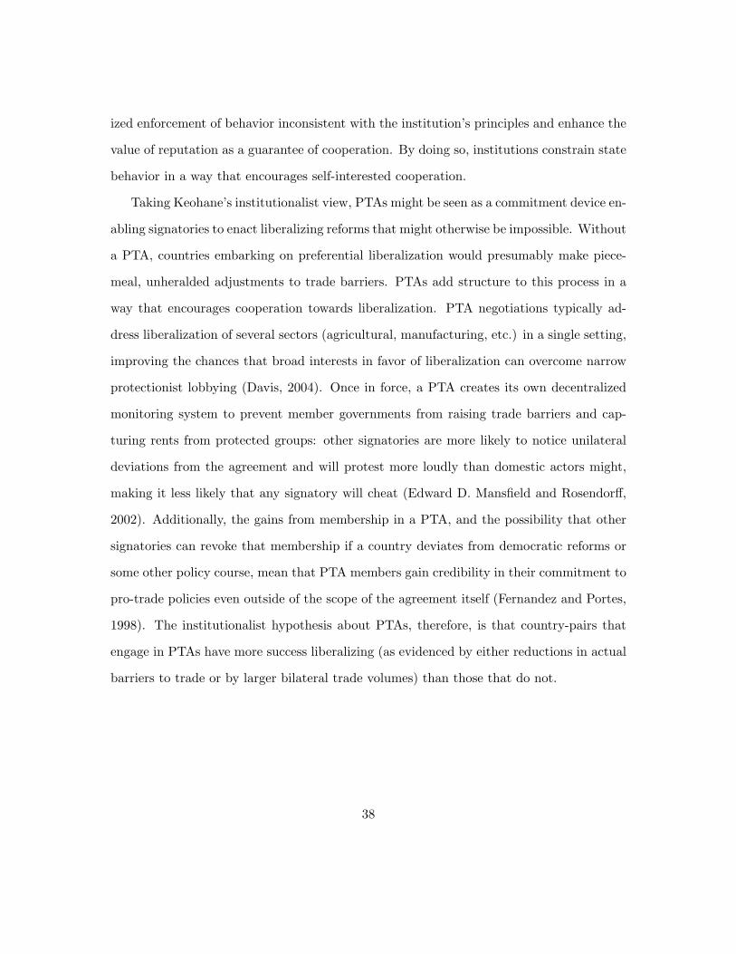
Taking Keohane’s institutionalist view, PTAs might be seen as a commitment device en-

abling signatories to enact liberalizing reforms that might otherwise be impossible. Without

a PTA, countries embarking on preferential liberalization would presumably make piece-

meal, unheralded adjustments to trade barriers. PTAs add structure to this process in a

way that encourages cooperation towards liberalization. PTA negotiations typically ad-

dress liberalization of several sectors (agricultural, manufacturing, etc.) in a single setting,

improving the chances that broad interests in favor of liberalization can overcome narrow

protectionist lobbying (Davis, 2004). Once in force, a PTA creates its own decentralized

monitoring system to prevent member governments from raising trade barriers and cap-

turing rents from protected groups: other signatories are more likely to notice unilateral

deviations from the agreement and will protest more loudly than domestic actors might,

making it less likely that any signatory will cheat (Edward D. Mansfield and Rosendorff,

2002). Additionally, the gains from membership in a PTA, and the possibility that other

signatories can revoke that membership if a country deviates from democratic reforms or

some other policy course, mean that PTA members gain credibility in their commitment to

pro-trade policies even outside of the scope of the agreement itself (Fernandez and Portes,

1998). The institutionalist hypothesis about PTAs, therefore, is that country-pairs that

engage in PTAs have more success liberalizing (as evidenced by either reductions in actual

barriers to trade or by larger bilateral trade volumes) than those that do not.

38

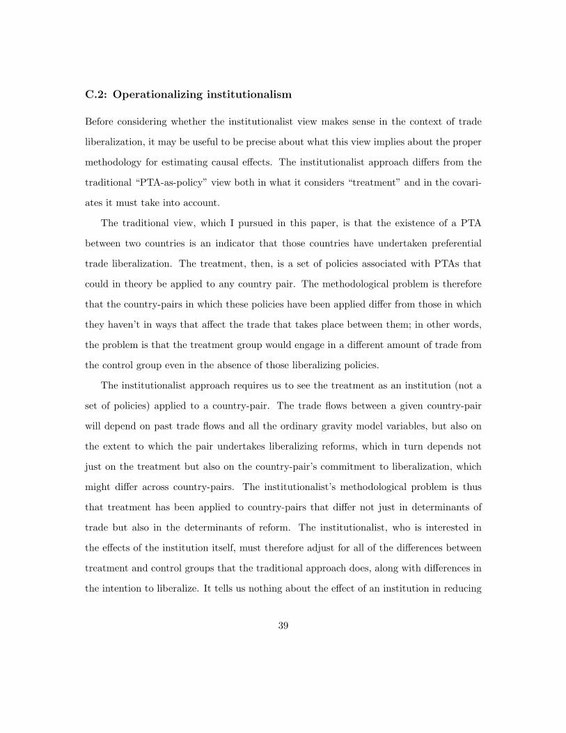
C.2: Operationalizing institutionalism

Before considering whether the institutionalist view makes sense in the context of trade

liberalization, it may be useful to be precise about what this view implies about the proper

methodology for estimating causal effects. The institutionalist approach differs from the

traditional “PTA-as-policy” view both in what it considers “treatment” and in the covari-

ates it must take into account.

The traditional view, which I pursued in this paper, is that the existence of a PTA

between two countries is an indicator that those countries have undertaken preferential

trade liberalization. The treatment, then, is a set of policies associated with PTAs that

could in theory be applied to any country pair. The methodological problem is therefore

that the country-pairs in which these policies have been applied differ from those in which

they haven’t in ways that affect the trade that takes place between them; in other words,

the problem is that the treatment group would engage in a different amount of trade from

the control group even in the absence of those liberalizing policies.

The institutionalist approach requires us to see the treatment as an institution (not a

set of policies) applied to a country-pair. The trade flows between a given country-pair

will depend on past trade flows and all the ordinary gravity model variables, but also on

the extent to which the pair undertakes liberalizing reforms, which in turn depends not

just on the treatment but also on the country-pair’s commitment to liberalization, which

might differ across country-pairs. The institutionalist’s methodological problem is thus

that treatment has been applied to country-pairs that differ not just in determinants of

trade but also in the determinants of reform. The institutionalist, who is interested in

the effects of the institution itself, must therefore adjust for all of the differences between

treatment and control groups that the traditional approach does, along with differences in

the intention to liberalize. It tells us nothing about the effect of an institution in reducing

39

trade barriers if we compare country-pairs that wanted to liberalize and formed a PTA and

those that did not want to liberalize and did not. In that case, we would have no way of

distinguishing between the role of the institution in constraining member behavior and its

role in selecting states interested in a certain kind of behavior.10

A slightly different way of illuminating this distinction is to compare the counterfactu-

als they employ. Both the traditional approach and the institutionalist approach can be

viewed as attempts to estimate trade flows for country pairs that adopted PTAs under the

counterfactual scenario in which they did not. Since the traditional approach views the

PTA as an indicator of preferential liberalization, it seeks to estimate what a country-pair’s

bilateral trade would be if it did not pursue preferential liberalization, which amounts to not

signing a PTA. The traditionalist can thus model trade for all country pairs that have not

entered into PTAs and use this model to estimate the counterfactual level of trade for pairs

that did.11 The institutionalist’s counterfactual is slightly different. The institutionalist

seeks to estimate what a country-pair’s bilateral trade would be if it pursued preferential

liberalization without the benefit of the PTA framework. Accordingly, she must somehow

account for intent to liberalize in her model of trade, and estimate counterfactual trade

flows for a country-pair with the same intent to liberalize but no PTA within which to do

it.

C.3: Evaluating the institutionalist approach in this context

I decided not to pursue the institutionalist approach for a few reasons. First, there is a

gap in the traditional empirical debate in economics for the use of matching techniques to10The difficulty of distinguishing between the constraining role of an institution – the way it structures

member behavior – and its screening role – the way it selects states with interests in a particular type ofbehavior – is discussed in Simmons and Hopkins (2005).

11The typical solution is to use regression analysis to account for those differences; as I have done here,it is also possible to use balancing methods, possibly in conjunction with regression methods.

40

reduce model dependence, and I want to try to fill that. Second, as I explain below, the

“intent to carry out preferential liberalization” may not be measurable, and at any rate is

harder to get at than “intent to liberalize,” which I also have not yet accounted for. Third,

it’s not clear how much preferential liberalization goes on outside of the framework of the

PTA, which might make this a bad place to exert effort in controlling for it.

How much significant preferential liberalization takes place outside of the structure of

a PTA? The defining principle of the GATT/WTO framework is nondiscriminatory trade,

epitomized by the practice of offering to each nation the trade privileges extended to the

“most favored nation. In that sense, preferential trade policies are against global trade

rules. The PTAs that member states report to GATT/WTO are an exception; GATT’s

founding principles allow for trade agreements that eliminate barriers to “substantially all

trade” among its members and does not “on the whole” increase protectionism against

non-members (Mansfield and Reinhardt, 2003, pp. 831–832). While only a subset of PTAs

meet these criteria, member states have continued to report PTAs to GATT/WTO and

the organization appears to turn a blind eye. The question, then, is to what extent states

maintain policies that favor particular nations but are not called PTAs and reported to

the GATT/WTO as such.

Frankel and Wei (1998, p. 191) mentions the “yen bloc” as an example of a “de facto

trade bloc in the absence of de jure trading arrangements,” but Frankel himself had already

elsewhere (1992) dismissed the idea; he showed that while trade within East Asian nations

increased in the 1980s, this was due to economic growth rather than an increasing intra-bloc

bias, and that there was no evidence of preferential policy.

Another scrap of evidence that preferential liberalization takes place is the frequency

of bilateral trade negotiations outside of the context of preferential trade agreements; the

high-profile US-Japan trade talks of the 1980s and early 1990s come to mind. If these talks

41

do not result in PTAs, what is the result? Were concessions granted in these talks granted

to all trading partners? It seems unlikely that trade negotiations would take this form if

the spoils were generally conferred.

If it is the case that PTAs represented the only substantial instance of preferential

liberalization, then the traditional and institutionalist estimates of the effect of PTAs on

trade would be identical. Formally, this would be because trade for the control group is

uncorrelated with desire for preferential liberalization (which is in turn because preferential

liberalization is uncorrelated with desire to liberalize), so estimating the counterfactual

amount of trade for country-pairs with PTAs does not require information about their

desire to liberalize.12 If there is preferential liberalization outside of PTAs but it is not

very significant, or if it is significant but not very correlated with PTA formation, then the

traditional estimate would again approximate the institutional answer. The institutionalist

would then be making the assertion that the adoption of this institution was random,

conditional on all the determinants of trade that the traditional approach employs, and

that all of the effect of PTAs on trade was due to the institution itself.

If, instead, preferential liberalization does take place outside of PTAs and is correlated

with PTA adoption, then the institutional estimate of the effect of PTAs on trade would

require information on desire for preferential liberalization. But here we must ask whether

there is a valid measure of this intention. As I discussed above, there are serious challenges

in measuring intention to liberalize generally, and my estimates above are probably some-

what biased by the failure to correct for this. Measuring in addition the intention to carry

out preferential liberalization seems impossible.

In conclusion, I think there is a lot of potential for employing methods developed in the

causal inference literature, including matching, to evaluate the institutionalist claim that12Note that we need to account for desire to generally liberalize either way.

42

international institutions can shape behavior and encourage cooperation, but for a number

of practical reasons I don’t believe that preferential trade agreements are an institution

where this approach can be pursued effectively.

43