Ashwini Jayaratnam

0

How Does The Black Market

Exchange Premium Affect

Foreign Direct Investment (FDI)?

Ashwini Jayaratnam

Email: ashwinij@stanford.edu

Advisor: Ronald McKinnon

Department of Economics, Stanford University

May 12, 2003

Abstract:

Throughout the 1970s and la te 1980s several developing countries tolerated black markets for foreign currency. The black market exchange premium is defined as the percentage difference between the black market rate for foreign currency and the pegged official exchange rate. While the effect of exchange rates on foreign direct investment (FDI) is a well-studied topic, the effect of the black market exchange premium on FDI is a less well-studied topic. Given the important role that FDI to developing countries plays in accelerating economic growth, studying the effect of the black market premium is relevant. In studying the effect of the black market premium I will be doing a historical study from 1982 to 1993, because black markets virtually disappeared in the mid-1990s as developing countries adopted liberalized currency regimes. If the black market premium is found to have affected FDI inflows during the period I will be studying, then it can be expected that the liberalization of currency regimes, and hence the disappearance of black markets, will impact FDI into developing countries in the future.

Ashwini Jayaratnam

1

1. Introduction∗

Foreign direct investment (FDI) is an important form of private external financing for

developing countries. Today, FDI is regarded as the major source of foreign capital for

developing countries, as opposed to portfolio flows or foreign aid. Unlike other major types of

private capital flows FDI is largely motivated by a firm’s long-term prospects for making profits

in production activities that it directly controls. Foreign bank lending and portfolio investment,

on the other hand, are motivated by short-term profit considerations. Since the 1980s, developing

countries’ share of total FDI inflows has risen significantly, from 26% in 1980 to 37% in 1997.

However, the distribution of FDI inflows among developing countries is uneven. In 1997, for

example, Asia received 22% of the share of total FDI inflows, Latin America and the Caribbean

received 14%, and Africa received 1%. The uneven dispersion of FDI is a cause for concern

since FDI is an important source of growth for developing countries. Not only can FDI add to

investment resources and capital formation, but it can also serve as an engine of technological

development with much of the benefits arising from positive spillover effects. Such positive

spillovers include transfers of production technology, skills, innovative capacity, and

organizational and managerial practices.

Recently, however, it has been claimed, based on empirical evidence, that the presence of

multi-national corporations (MNCs) in developing countries do not bring the expected positive

spillover effects to domestic firms in the same industry. In fact, there are often negative spillover

effects as domestic firm productivity decreases as MNCs move into the market. The fall in

domestic productivity is attributed to domestic firms having to compete with more efficient

MNCs. Going by such evidence it might seem that FDI is unimportant, and even an obstacle, for

∗ I would like to thank my thesis adviser, Ronald McKinnon, for his interest and help in formulating the project. I would also like to Geoffrey Rothwell for providing support and motivation throughout the thesis writing process.

Ashwini Jayaratnam

2

economic growth in developing countries. However, further studies have argued that while there

might not be evidence for positive intra- industry spillovers, meaning spillovers for domestic

firms operating in the same industry as MNCs, there is evidence for positive inter-industry

spillovers, meaning spillovers that accrue to domestic firms in different industries. Such inter-

industry spillovers are often attributed to the cross-fertilization of ideas through knowledge-

sharing. Maurice Kugler uses empirical evidence on manufacturing in Colombia to illustrate this

point (2001). He asserts that producers in other sectors may experience positive spillovers

especially when MNCs outsource to local upstream suppliers. Therefore, FDI has to potential to

boost the economies of developing countries through knowledge-sharing and technology transfer

between industries.

Given the potential role that FDI can play in accelerating growth, studying its

determinants in developing countries is important and relevant to understanding how FDI may be

attracted. In fact many developing countries today are trying to make their business environment

more attractive to foreign investors through establishment of a hospitable regulatory framework

for FDI. Relaxing rules regarding market entry and foreign ownership, improving standards of

treatment accorded to foreign firms, and improving the functioning of markets are some ways of

doing this. In addition to seeking a hospitable business climate, firms that invest abroad often

factor in the size of the local market and cost of resources, such as labor and capital, in the local

market. To this extent countries where labor costs are cheap relative to industrialized countries

are successful in attracting FDI. Several Southeast Asian, such as Indonesia and Malaysia, fall

into this category. While low-labor costs and large markets are important determinants of FDI,

the role of exchange rates in influencing FDI inflows has become a well-studied topic since the

1990s. The level of the exchange rate and exchange rate volatility are both thought to be

Ashwini Jayaratnam

3

determinants of foreign investment. However, the direction in which exchange rate levels and

exchange rate volatility impact FDI flows is far from certain.

The emphasis placed on exchange rates in determining FDI flows gives rise to my

research question, which is how the black market exchange premium affects foreign investment.

The black market exchange rate is the price of foreign currency on the black market. The

premium is defined as the percentage difference between the black market rate and the official

exchange rate. Black markets for foreign exchange were prominent in several developing

countries in Asia, Latin and Central America and Africa throughout the 1970s and early 1990s,

because during these periods currency regimes were not liberalized and governments imposed

controls on obtaining foreign exchange. Exchange controls were intended to insulate

international reserves from depletion, which is a problem under pegged exchange rate regimes

when the value of the currency is falling. There have been several studies on the effectiveness of

black market in protecting international reserves and fighting inflation, as well as on the

determinants of the black market premium. However, as far as I am aware there have been no

studies on how the black market premium might affect FDI. This is interesting in light of the fact

that there are several studies on the effect of exchange rates on FDI, and it is well known that

exchange rates and the black market premium are closely linked.

In looking at how the black market premium affects FDI, I will be doing a historical

study for the years 1982 to 1993. The reason for doing a historical study is that today most

developing countries are moving towards liberalized exchange rate regimes, where their currency

is allowed to float on the market. Floating exchange rate regimes make black markets

unnecessary. Given that black markets virtually disappeared in the early and mid 1990s, when

developing countries sought to transform several of their economic policies, my study ends in

Ashwini Jayaratnam

4

1993. The reason for starting in 1982, despite black markets being present in the 1970s, is that

FDI to developing countries only started to come in during the 1980s. The results of my study

should shed light on whether black markets served to impede or enhance FDI inflows, and hence

whether their disappearance since the 1990s should be of importance to developing countries

keen to attract FDI.

2. Literature Review

2.1 The Black Market Exchange Rate:

To better explain the black market exchange rate system, I will briefly review conceptual

distinctions among different foreign exchange rate regimes. A uniform fixed exchange rate

system entails one pegged exchange rate applying to all transactions. A uniform flexible

exchange rate system also entails a single market for foreign exchange, however, under this

system the exchange rate varies according to demand and supply conditions. Unlike a uniform

exchange rate regime, a dual exchange rate regime is a system created by the authorities under

which there are two officially accepted exchange rates. An official rate, which is pegged, exists

for certain transactions, and a parallel rate, which is market determined, exists for other

transactions. Usually the official rate applies to current account transactions while the parallel

rate applies to capital account transactions. Dual exchange rate regimes are common in

developing countries, and their objective is to avoid the short-term effects of a depreciation of

the exchange rate on domestic prices while maintaining some degree of control over capital

outflows and international reserves (Kiguel, Lizondo, O’Connell, 1997).

Ashwini Jayaratnam

5

Under a uniform pegged exchange rate system the market for foreign exchange clears

through changes in international reserves, and thus there is the danger of large capital outflows

depleting international reserves. A dual rate system solves this problem because capital outflows

lead to a depreciation of the parallel rate instead of a large loss in reserves. Also under a uniform

floating exchange rate system, where the official exchange rate market clears through

movements in the exchange rate, capital outflows can have large impacts on domestic prices.

Dual exchange rate systems can help mitigate the effects of these price shocks, for under a dual

rate system current account transactions are usually pegged at the official rate. Thus, in principle,

dual rate systems should maintain external balance by insulating international reserves from

capital outflows, and control inflation by having current account transactions conducted at the

pegged exchange rate.

Black market exchange rate systems are in some respects similar to dual rate systems. As

in a dual rate system, under a black market exchange rate regime there are two exchange rates.

However, while the two exchange rates under a dual rate system are created by the authorities,

black markets are not sanctioned by the authorities and instead arise due to the imposition of

exchange controls. Exchange controls are imposed by governments to protect international

reserves. Controls on access to foreign exchange create excess demand that needs to be satisfied

at a premium in a second market thus giving incentives for the emergence of a black market for

foreign currency. Under a pegged exchange rate regime with exchange controls there is no

mechanism to clear the official exchange rate market, for international reserves are protected by

exchange controls. As a result, black markets play the role of clearing transactions that are not

sanctioned in the official market. To this extent black markets serve to correct a market failure

that causes excess demand.

Ashwini Jayaratnam

6

2.2 Determination of the Black Market Exchange Rate

The portfolio balance model is frequently tested to study the determinants of the black

market exchange rate. In this model relative asset supplies and expectations of future exchange

rate developments play a crucial role in determining the black market exchange rate. The basic

idea in the portfolio balance model is that foreign exchange is regarded as an asset, and portfolio

decisions emphasize holding black market dollars versus domestic assets. Fears about inflation,

low domestic interest rates, as well as political and economic instability, give rise to demand for

foreign currency in the black market. Dornbusch (1983) uses the portfolio balance model to

study determinants of the black market exchange rate in Brazil and Saca (1997) used a similar

approach for El Salvador. The portfolio balance approach is relevant for countries where black

markets exist, due to exchange controls, but only come into prominence in the face of serious

balance of payments crises. Under these circumstances portfolio diversification represents a key

determinant of the demand for foreign exchange on the black market. Such was the case in El

Salvador where the black market existed since the 1960s but only became important in the 1980s

when the country faced a serious balance of payments deficit. Also, the portfolio balance

approach is relevant for countries that impose restrictions on private capital outflows. Again, this

has been the case for El Salvador since the 1980s (Saca1997).

Dornbusch’s (1983) study emphasizes portfolio decisions on holding black market dollars

versus domestic assets for the case of Brazil. His model explains how changes in financial and

real variables, as well as expectations of future exchange rate movements, affect the black

market rate. For example, a tight monetary policy, by raising domestic interest rates, increases

the relative attractiveness of domestic assets. In this case higher demand for domestic assets

relative to foreign assets reduces the black market premium.

Ashwini Jayaratnam

7

A real depreciation of the official exchange rate also reduces the premium. Expectations

of a future devaluation of the official exchange rate initially increase the premium due to the

black market rate depreciating in anticipation of the coming devaluation of the official rate.

However, once the devaluation actually takes place the premium decreases. In the case of Brazil,

the premium is also affected by seasonal increases in the supply of black market foreign

exchange due to tourism. Tourists increase net inflows of foreign exchange and thus reduce the

black market exchange rate, which is determined according to supply and demand conditions.

Thus in Dornbusch’s (1983) study of the determinants of the black market premium in Brazil, the

main explanatory variables are the real official exchange rate, the interest rate differential, and

seasonal factors related to tourism.

Saca (1997) uses a similar approach to study the determinants of the black market

premium in El Salvador. Saca starts from the premise that since the black market rate is

determined according to supply and demand conditions, for the market to clear the supply of

foreign exchange on the black market has to equal the demand. Saca posits that the supply of

foreign exchange depends on the black market premium, the official exchange rate and seasonal

factors. A higher premium increases supply, because a higher price can be obtained for the

foreign exchange supplied. A more depreciated official exchange reduces the supply of foreign

exchange, as excess demand for foreign exchange is reflected in the higher price embodied by

the official rate. Seasonal inflows of remittances, which occur during Christmas, naturally

increase the supply of foreign exchange.

The determinants of demand include the black market premium, the level of real income,

the money supply, the depreciation-adjusted interest differential, and expectations of changes in

economic policy or government reform, each affect the demand for foreign exchange on the

Ashwini Jayaratnam

8

black market. An increase in the black market premium, which reflects a higher price for foreign

exchange on the black market, reduces demand. An increase in real income and an increase in

the domestic money supply each increase demand. The former effect is the result of more money

leading to greater demand for foreign exchange, while the latter effect arises because an increase

in the domestic money supply lowers domestic interest rates thereby making foreign assets more

attractive relative to domestic ones. The variable for the depreciation-adjusted interest

differential uses the El Salvador interest rate as the domestic one and the US interest rate as the

foreign one. As the interest differential rises, meaning that domestic interest rates go up relative

to foreign ones, demand for foreign exchange goes down. Lastly, expectations of a change in

economic policy or government reform are thought to increase demand.

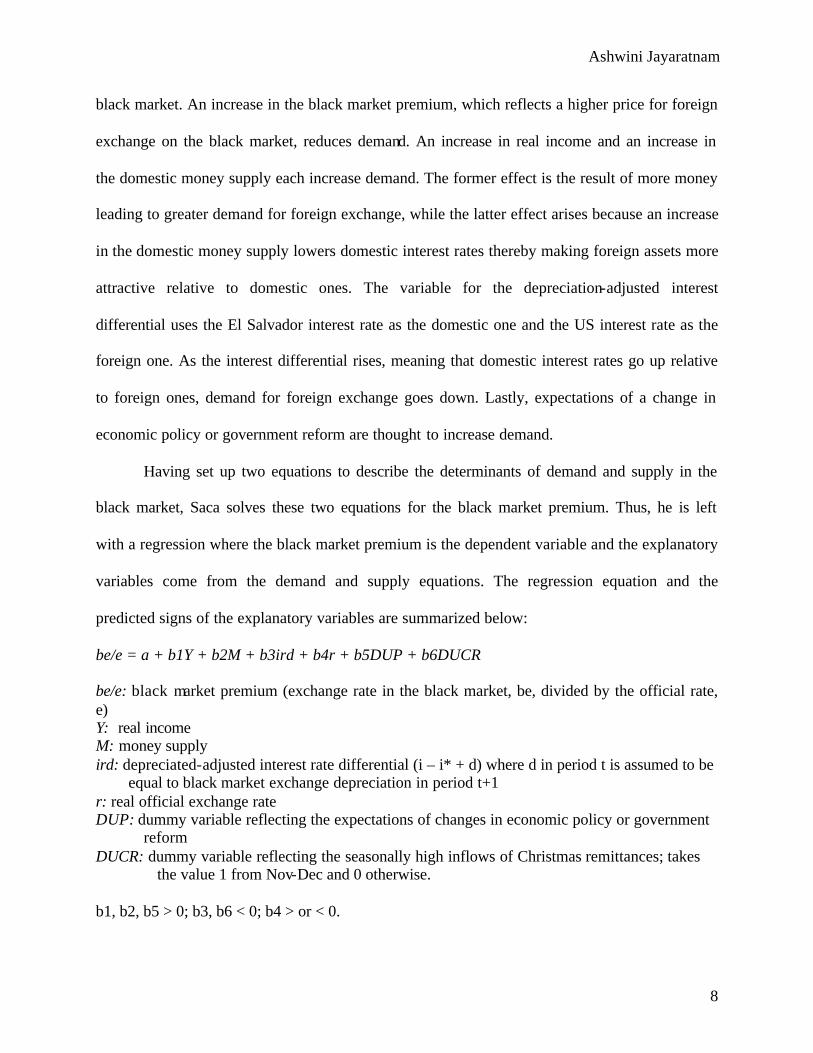
Having set up two equations to describe the determinants of demand and supply in the

black market, Saca solves these two equations for the black market premium. Thus, he is left

with a regression where the black market premium is the dependent variable and the explanatory

variables come from the demand and supply equations. The regression equation and the

predicted signs of the explanatory variables are summarized below:

be/e = a + b1Y + b2M + b3ird + b4r + b5DUP + b6DUCR

be/e: black market premium (exchange rate in the black market, be, divided by the official rate, e) Y: real income M: money supply ird: depreciated-adjusted interest rate differential (i – i* + d) where d in period t is assumed to be equal to black market exchange depreciation in period t+1 r: real official exchange rate DUP: dummy variable reflecting the expectations of changes in economic policy or government reform DUCR: dummy variable reflecting the seasonally high inflows of Christmas remittances; takes the value 1 from Nov-Dec and 0 otherwise. b1, b2, b5 > 0; b3, b6 < 0; b4 > or < 0.

Ashwini Jayaratnam

9

As can be seen Saca is uncertain regarding the sign on the coefficient for the real official

exchange rate. A depreciation in the official rate reduces the supply of foreign exchange on the

black market, which can increase the premium. However, the black market premium may also

decline with an official devaluation if the reduction in demand, due to the higher official price

for foreign currency, is enough to offset the reduction in supply in the black market.

The empirical results of Saca’s study reveal that a 1% real depreciation of the official

exchange rate leads to a proportional decline in the premium. Such a finding seems consistent

with the hypothesis that the black market premium may rise in the face of expectations of a

future devaluation in the official rate, and then fall once the devaluation actually takes place.

Also, the negative sign on the coefficient for the official exchange rate might signify that

depreciation increases receipts of official foreign exchange, through increased exports, and

therefore lowers the demand for foreign exchange in the black market, which leads to a fall in the

premium. An increase in the U.S. interest rate relative to the rate in El Salvador leads to an

increase in the premium. This is in accordance with the theory that higher interest rates on

foreign assets make them more attractive and thus increase the price of foreign currency. Higher

expectations regarding changes in economic policy or government reform lead to an increase in

the premium, and greater inflows of foreign exchange through remittances during the Christmas

season reduce the premium. Both these results are in accordance with the hypotheses set forth.

The only variable in the regression which behaves contrary to theory is the money supply. An

increase in the money supply was predicted to increase the premium, for a looser monetary

policy meant lower domestic interest rates, which make foreign assets more attractive than

domestic ones, and through this increased demand for foreign exchange the premium rises.

However, the coefficient on the money supply is negative, meaning that an increase in the money

Ashwini Jayaratnam

10

supply actually reduces the premium. Saca explains this by suggesting that perhaps the

authorities reduced the money supply when the premium was high. This suggests a causal

relationship from the exchange rate to the money supply.

2.3 FDI and Exchange Rates

The effect of exchange rate movements on FDI flows is a fairly well studied topic,

although the direction and magnitude of influence is far from certain. However, the effect of the

black market premium on FDI flows has been less studied. The literature relating FDI and

exchange rate movements will be a useful starting point from which to study the black market

premium and FDI, so as to later predict the relationship between the two.

Exchange rate movements and exchange rate uncertainty would appear to be important

factors investors take into account when making the decision to invest abroad. Yet one might

argue that if exchange rate movements offset price movements so that purchasing power parity is

maintained, then there should be little effect on FDI flows. However, empirical evidence shows

that purchasing power parity does not hold for all time periods and thus exchange rate

movements are important in determining the flow of FDI. Much of the literature on exchange

rate movements and FDI concentrates on two issues: the level of the exchange rate, and the

volatility of the exchange rate.

2.31 Exchange Rate Levels

Froot and Stein (1991) claimed that the level of the exchange rate may influence FDI,

because depreciation of the host country currency against the home country currency increases

the relative wealth of foreigners thereby increasing the attractiveness of the host country for FDI

as firms are able to acquire assets in the host country relatively cheaply. Thus a depreciation of

Ashwini Jayaratnam

11

the host currency should increase FDI into the host country, and conversely an appreciation of

the host currency should decrease FDI. Against this argument, it is often claimed that the price of

assets should not matter but only their rate of return. When the host country currency depreciates

relative to the home country currency, not only the price, but also the nominal return of the assets

in the host country currency goes down. Since prices of assets and returns on assets both go

down exchange rate movements should not affect FDI. Froot and Stein (1991) counter this

argument with the claim that when capital markets are subject to information imperfections,

exchange rate movements do in fact influence foreign investment. Information asymmetry causes

a divergence between internal and external financing, making the latter more expensive than the

former, since the lenders incur monitoring costs and thus lend less than the full value of the asset.

In this environment should foreign investors hold their wealth in foreign currency, then

depreciation of the local currency will increase the wealth position of foreign agents relative to

domestic agents, thus leading foreign investors to bid more aggressively for domestic assets.

Froot and Stein (1991) use industry-level data on US inward FDI for the 1970s and 1980s to

support their hypothesis.

Contrary to Froot and Stein (1991), Campa (1993) puts forth the hypothesis that an

appreciation of the host currency will in fact increase FDI into the host country. Instead of

focusing on the price of foreign assets, as did Froot and Stein, Campa’s approach is more along

the lines of a production based theoretical approach. According to Campa, a firm’s decision to

invest abroad depends on its expectations regarding future profit streams. An appreciation of the

host currency increases expectations of future profitability in terms of the home currency. Campa

analyzes the number of foreign entrants to the US in the 1980s to provide evidence for his claim.

Ashwini Jayaratnam

12

In accordance with his hypothesis, Campa finds that an appreciation in the host-country

exchange rate stimulates FDI to the host-country.

An important study by Blonigen (1997) on exchange rate levels and FDI shows that real

dollar depreciations increase foreign acquisitions involving firm-specific assets by foreign firms.

To illustrate this claim Blonigen uses data on Japanese acquisitions in the US from 1975 to 1992.

The argument that real dollar depreciations increase foreign acquisitions that is put forth by

Blonigen differs from the argument put forth by Froot and Stein (1991), although they both have

the same outcome. Froot and Stein show that exchange rate movements are important because

capital markets are imperfect. On the other hand, Blonigen shows that exchange rate movements

matter because while domestic and foreign firms may have the same opportunities to purchase

firm-specific assets in the domestic market, foreign and domestic firms do no have the same

opportunities to generate returns on these assets in foreign markets. Due to the unequal level of

access to markets, exchange rate movements may affect the relative level of foreign firm

acquisitions. Blonigen makes the point that assets related to FDI should not be considered similar

to assets such as bonds. A feature of an asset similar to a bond is that the price and nominal

return are in the same currency regardless of the investor. However, such is not the case with

assets related to FDI for the assets of a target firm can be in the form of firm-specific assets,

which can generate returns simultaneously in several markets without involving any foreign

currency transactions.

Having discussed why exchange rate movements are important when domestic and

foreign markets are segmented and acquisitions are firm-specific, Blonigen goes on to describe

the empirical tests to support his claim. As mentioned before, Blonigen focuses his research on

Japanese acquisitions in the US from 1975 to 1992. Such a focus is chosen because of two

Ashwini Jayaratnam

13

important considerations that are specific to the market structure of Japan and the US. First, the

hypothesized link between exchange rate movements and acquisition FDI depends on the extent

to which domestic and foreign markets are segmented, meaning that relative to foreign firms

domestic firms have limited access to the foreign market. The Japanese market is known to have

been well insulated from imports and FDI, the result being that there are relatively few foreign

firms in the Japanese market compared to domestic ones. Second, the link between exchange rate

movements and acquisition FDI is conditioned on the basis that the acquisitions involve firm-

specific assets. Here again past studies have shown that Japanese acquisition FDI into the US is

motivated by the desire to possess technology related firm-specific assets. Thus, the presence of

segmented markets and firm-specific assets make studying acquisition FDI between Japan and

the US relevant.

In Blonigen’s (1997) model the probability of a foreign firm acquiring a US is a function

of the industry-specific real exchange rate. The dependent variable is therefore the number of

Japanese acquisitions into the US. An increase in the industry-specific real exchange rate

represents a real depreciation of the dollar relative to the yen. According to Blonigen’s

hypothesis, this should mean that there is a positive correlation between the real exchange rate

and Japanese acquisitions. In order to account for other factors that are likely to affect Japanese

acquisitions, Blonigen includes a set of explanatory variables in the regression. To capture

overall industry activity and target firm supply in the US, Blonigen includes as a variable the

number of acquisitions of US target firms by other US firms. Since a high number of such

acquisitions is indicative of a high supply of US target firms, a positive correlation with the

number of Japanese acquisitions is expected. Indeed, the empirical results show that the supply

factor is positively correlated with the level of Japanese acquisitions. Blonigen also uses a

Ashwini Jayaratnam

14

number of proxies for Japanese demand, as well as measures of protectionism and economy-

wide growth. He finds that high levels of demand in Japan are positively correlated with the level

of acquisition. However, surprisingly, he find that the level of protection does not have a

statistically significant effect, This result is contradictory to the general view that FDI flows

accelerate to markets that are difficult to penetrate through imports.

Regarding the exchange rate, there is a statistically significant and positive relationship

with Japanese acquisition activity, which is in line with Blonigen’s prediction. However, despite

showing such a result, it remains unclear whether the correlation between exchange rate

movements and Japanese acquisition FDI is due to the presence of firm-specific assets

(Blonigen’s claim and one of the conditions discussed earlier) or due to the hypothesis put forth

by Froot and Stein (1991), which is imperfect capital markets. To test this question Blonigen

separates acquisitions into those in the manufacturing industry and those in the non-

manufacturing industry. The reason for separating acquisitions in such a way is that firm-specific

assets are said to be more important in the manufacturing industry. Indeed, Blonigen finds that

the coefficient on the real exchange rate for non-manufacturing industries is statistically

insignificant while the coefficient for manufacturing industries is significant. Next, Blonigen

divides acquisitions within the manufacturing industry into those involving high R&D

expenditures, as a percentage of sales, and those involving low R&D expenditures. Since

Japanese firms may be particularly interested in technology related, firm-specific assets, where

high R&D expenditures are important, exchange rate movements should influence acquisition

FDI more in industries with high R&D expenditures. The result of running regressions on high

and low R&D manufacturing industries showed that the coefficient on the real exchange rate

variable is insignificant for the low R&D sample and significant for the high R&D sample. Thus

Ashwini Jayaratnam

15

it can be seen that through separating Japanese acquisitions into those in the manufacturing and

non-manufacturing industries, and then further splitting the ones within manufacturing into high

and low R&D samples, Blonigen is able to support his claim that exchange rate movements

influence FDI due to firm-specific assets.

2.32 Exchange Rate Volatility

Regarding exchange rate volatility, the theoretical arguments linking volatility to FDI

have been divided between production flexibility arguments and risk-aversion arguments.

According to production flexibility arguments, exchange rate volatility increases foreign

investment because firms can adjust the use of one of their variable factors following the

realization of nominal or real shocks. It can be seen that the production flexibility argument

relies on the assumption that firms can in fact adjust variable factors, for the argument would not

hold if factors were fixed. According to the risk aversion theory FDI decreases as exchange rate

volatility increases. Higher volatility in the exchange rate lowers the certainty equivalent

expected exchange rate. Certainty equivalent levels are used in the expected profit functions of

firms that make investment decisions today in order to realize profits in future periods (Goldberg

and Kolstad 1995). Campa (1993) extends this claim to include risk-neutral firms by using the

argument of future expected profits. Investors are concerned with future expected profits and

because of exchange rate volatility firms may temporarily postpone the decision to invest abroad,

as they would prefer to invest in a country where due to stable exchange rates their expected

profits are less volatile. This theoretical result is confirmed using data for inward investment to

the US in the wholesale industries in the 1980s. Goldberg and Kolstad (1995) note that when

evaluating risk-aversion approaches versus production flexibility approaches it is important to

distinguish between short-term exchange rate volatility and long-term misalignments. Under

Ashwini Jayaratnam

16

short-term volatility risk-aversion arguments are more convincing because firms are unlikely to

be capable of adjusting factors in the short-run, where factors of production are usually fixed,

and as a result firms will only be risk-averse to volatility in their future profits. However, in the

case of long-term misalignments, the production flexibility argument appears more convincing as

firms are now able to adjust their use of variable factors.

Cushman (1985) modifies the analys is based on production flexibility and risk-aversion

arguments to develop a framework where firms choose between serving foreign markets via

exports or via FDI. Under exchange rate volatility, Cushman hypothesizes that firms will prefer

FDI to exports, and thus increased exchange rate volatility leads to increased FDI. He uses data

on US outward FDI in five OECD countries for the years 1963-78 to confirm his claim.

However, contrary to Cushman, a similar study by Sercu and Vanhulle (1992) shows that

increased volatility in exchange rates raises the returns to exports thereby reducing levels of

foreign investment. When firms are not faced with a choice between exporting and FDI, the

effect of exchange rate volatility on FDI changes.

As can be seen, the effects of both the exchange rate level and exchange rate volatility on

FDI are ambiguous. A recent study by Gorg and Wakelin (2002) on both outward US foreign

investment in 12 developed countries and inward investment to the US from those same

countries for the period 1983 to 1995 provides further evidence on the issue. The level of the real

exchange rate (partner currency per US dollar) is calculated as the log of the annual mean of the

monthly exchange rates for a given year. Exchange rate volatility is measured by the standard

deviation of the exchange rate and is calculated as the annual standard deviation of the log of the

monthly changes in the exchange rate. Controlling for labor costs, relative interest rates, partner

country GDP, US GDP, freight costs, distance between the partner country and the US, and

Ashwini Jayaratnam

17

finally language, which is a dummy variable that is equal to1 if the official language is English

and 0 otherwise, Gorg and Wakelin find that exchange rate volatility has no effect on US

outward FDI. Such a finding runs contrary to past studies, including Cushman’s model of the

choice between FDI and exports under exchange rate volatility and Campa’s extension of the

standard model, where there is no choice between exports and FDI, to include risk-neutral firms.

However, the level of the exchange rate has a negative effect coefficient, thus implying that the

level of US outward FDI increases with an appreciation of the host country exchange rate. Such

a result is in line with the previous study by Campa (1985) where he hypothesized and provided

empirical evidence for the claim that an appreciation of the host country exchange rate increases

a multinational firm’s expectations of future profitability in home currency terms and thereby

increases foreign investment.

Regarding inward FDI to the US, Gorg and Wakelin (2002) find that exchange rate

volatility has no statistically significant effect on inward FDI, which is consistent with the

finding regarding outward US FDI. The level of the exchange rate is shown to negatively affect

inward FDI. This means that inward FDI increases as the foreign currency appreciates against

the dollar. This results is in line with that of Froot and Stein (1991) who claimed that foreign

investment increases as the host country currency depreciates, for relative asset prices in the host

country become cheaper. It also in line with Blonigen’s (1997) claim regarding firm-specific

assets. However, such a result is at the same time contrary to Gorg and Wakelin’s (2002) own

finding on the effect of the exchange rate level of outward FDI, which showed that outward US

foreign investment decreased as the host country currency depreciated against the dollar.

Ashwini Jayaratnam

18

2.4 Additional Economic Determinants of FDI

More general studies on the determinants of FDI highlight some of the factors that in

theory should influence foreign investment and at the same time shed further light on the

relationship between FDI and exchange rates. Barrell and Pain (1996) construct a model of direct

investment in which multinational firms seek to maximize the current discounted value of

profits, which are determined by sales revenue and production costs in both domestic and foreign

markets. Costs, in both the domestic and foreign markets, are capital and labor costs. Moreover,

the authors claim that costs incurred in foreign markets, through investment, are positively

related to demand in the foreign market. For instance, with regard to foreign investment in

manufacturing, investing in facilities such as after-sales repair and maintenance outlets raises the

level of demand for manufactured products. This means that sales revenue generated abroad is

endogenous with respect to investment abroad.

From the theoretical profit-maximizing model Barrell and Pain (1996) derive the reduced

form of an econometric equation in which the dependent variable is the outward flow of U.S.

foreign investment. The sample period used runs from 1971Q1-1988Q4. The explanatory

variables in the regression, which spring from the theoretical model, are domestic and foreign

demand, capital costs and labor costs. The other variables added to the regression are volume of

exports from the home country (which in Barrell and Pain’s model is the U.S.), real level of U.S.

corporate profits, the dollar exchange rate and a dummy variable for exchange controls. In

studying the effect of the exchange rate (units of foreign currency per unit of domestic currency)

Barrell and Pain (1996) look at expectations of short-term changes in the exchange rate.

Expectations of short-term changes in the exchange rate are regarded as important for it is

hypothesized that companies may speed up payments in currencies expected to appreciate,

Ashwini Jayaratnam

19

thereby increasing foreign investment flows. Conversely it should be the case that an expected

depreciation of the foreign currency will postpone investment as companies delay payments in

expectation of future currency gains. To account for the importance of expectations of future

movements in the exchange rate the difference between the forward and spot rate is entered into

the regression. The regression results showed that an expected appreciation in the dollar, or

equivalently an expected depreciation of the foreign currency, would temporarily postpone

investment. This result is consistent with the hypothesis put forward by Barrell and Pain (1996).

Love and Lage-Hidalgo (2000) develop a model to examine the determinants of foreign

investment by testing investment flows from the US to Mexico between 1967 and 1994. One of

their main objectives was to find out whether US FDI flows into Mexico are determined solely

by a cheap labor effect boosted by the maquiladora industrialization program1 or whether the

Mexican market itself provides incentives for inward FDI, as would be expected due to the

market size hypothesis. Love and Lage-Hidalgo start with a theoretical model of the factors that

should drive FDI. In choosing the correct level of foreign production, firms seek to minimize

their total production costs, comprised of foreign and domestic production costs, subject to a

total demand constraint, where total demand is comprised of foreign and domestic demand. Once

the level of foreign production has been chosen firms must choose the optimal factor mix,

comprised of labor and capital. Firms thus minimize labor costs, wages, and capital costs subject

to a demand constraint in choosing the optimal capital stock. Flows of FDI will be a lagged

function of the difference between actual and desired capital stocks in previous periods. Thus,

altogether the flow of FDI depends on both the determinants of the optimal capital stock, which

1 The maquiladora industrialization program allowed companies setting up maquiladoras to import raw materials and equipment without tariffs. The components made in maquiladoras were then exported to factories in the U.S., where they were assembled into final products. The program was intended to give incentives for multinational firms to relocate their manufacturing plants to Mexico where they could take advantage of cheap labor.

Ashwini Jayaratnam

20

are demand and unit cost differentials between the home and foreign country, and on the lagged

value of actual foreign capital stock.

According to the results, a higher per capita GDP, which proxies demand, is positively

correlated with FDI flows. Also, as US wages go up relative to those in Mexico, FDI flows

increase. The theoretical model developed by Love and Hidalgo predicts both these results. The

stock of US direct investment lagged one year has a negative sign as expected for if the actual

stock is closer to its desired level then less investment is necessary. However, the coefficient is

not statistically significant at the 5% level. Contrary to theory, the coefficient on the relative user

cost of capital is negative, indicating that FDI from the US to Mexico decreases as the US cost of

capital rises relative to that of Mexico. Two explanations for this contradiction are given. The

first comes from an earlier hypothesis put forth by Cushman (1985) when trying to explain a

similar result for overall US FDI flows between 1963 and 1981. Cushman claims that a high host

country cost of capital causes increased domestic financing of foreign capital, thus raising FDI.

The second explanation relates to differential interest rates and was put forth by Calvo,

Leiderman and Reinhart (1993), who pointed out that the sharp decline in US short-term interest

rates in the early 1990s was accompanied by a large capital inflow into Latin America. The

reason for this apparent correlation is that reduced US interest rates lead to improved solvency of

Latin American debtors, thus providing an incentive for repatriation of capital held in the US and

for increased borrowing by Latin American sources from US capital markets.

While the real exchange rate never enters into the theoretical FDI model developed by

Love and Hidalgo (2000), they acknowledge that exchange rate movements may affect FDI

flows, and thus incorporate a real exchange rate variable into their regression model. Following

Froot and Stein (1991), they hypothesize that a depreciation in the peso relative to the dollar

Ashwini Jayaratnam

21

should increase US investment in Mexico, because of the decrease in the dollar cost of acquiring

Mexican assets. However, Love and Hidalgo (2000) are concerned with the effect of exchange

rate movements on the timing of investment flows, and thus include a one period lagged variable

for changes in the real exchange rate, rather than a variable for changes in the exchange rate for

the current period. The results show that the coefficient on the lagged variable is positive

meaning that a depreciation of the peso encourages US direct investment in Mexico. This

suggests that the mechanism outlined in Froot and Stein (1991) operates with a time delay.

3. Model

The purpose of this investigation is to test the effect of the black market exchange

premium on flows of FDI. This relationship will be tested using data from developing countries

with high, low and moderate black market premiums for the years 1982-1993. Black markets for

foreign exchange were prominent from approximately 1970 to 1994, after which most

developing countries adopted liberalized exchange rate regimes, thus making black markets

unnecessary. Hence, examining the effect of the black market premium on FDI flows is a

historical study. If the black market premium negatively impacted FDI flows, then a move to

liberalized exchange rate regimes, eliminating the need for black markets, should help

developing countries attract FDI. The reason for not testing the relationship between the

premium and FDI flows from 1970-1994, and instead starting in 1980, is that FDI to developing

countries became significant only in the 1980s.

Examples of countries that had low premiums between 1970 and 1994 are Thailand,

Malaysia, Indonesia, Mexico and France. The average premium for countries with low premium

Ashwini Jayaratnam

22

ranges from 1.7% to 3.7%. Several Latin American countries belong to the group classified as

having moderate premiums, which range from 9.4% to 24.6%. Some examples of such countries

are Bolivia, Ecuador, Argentina, Brazil and Chile. Lastly, countries classified as having high

premiums are mostly African countries including Sudan, Ghana, Nigeria, and Zambia. This

group of countries has premiums ranging from 85.4% to 99.8%.

3.1 Economic Model

A firm’s decision to invest abroad hinges on whether foreign production is profit

maximizing and therefore the economic determinants of FDI derive from the extent to which the

factors accounted for make foreign investment profitable. In formulating an econometric model

for the determinants of FDI, I will start from a theoretical model put forth by Love and Lage-

Hidalgo (2000). Love and Lage-Hidalgo’s model of FDI comes from a paper where they analyze

the determinants of U.S. direct investment in Mexico in an effort to understand whether market

size or production cost differential between the home and the host country drive FDI. Instead of

approaching the foreign investment decision through profit maximization, Love and Hidalgo

approach it through cost minimization, which in theory should lead to the same optimal level of

foreign investment as the profit maximization approach. Under the cost minimization model

firms must first decide the appropriate level of foreign production and subsequently select the

appropriate input mix for this level of foreign production.

Total production costs are equal to total costs for domestic production plus total costs for

foreign production. Thus, if domestic and foreign production are labeled as D and F,

respectively, then total production costs can be written as:

TC = TCD + TCF (1)

Ashwini Jayaratnam

23

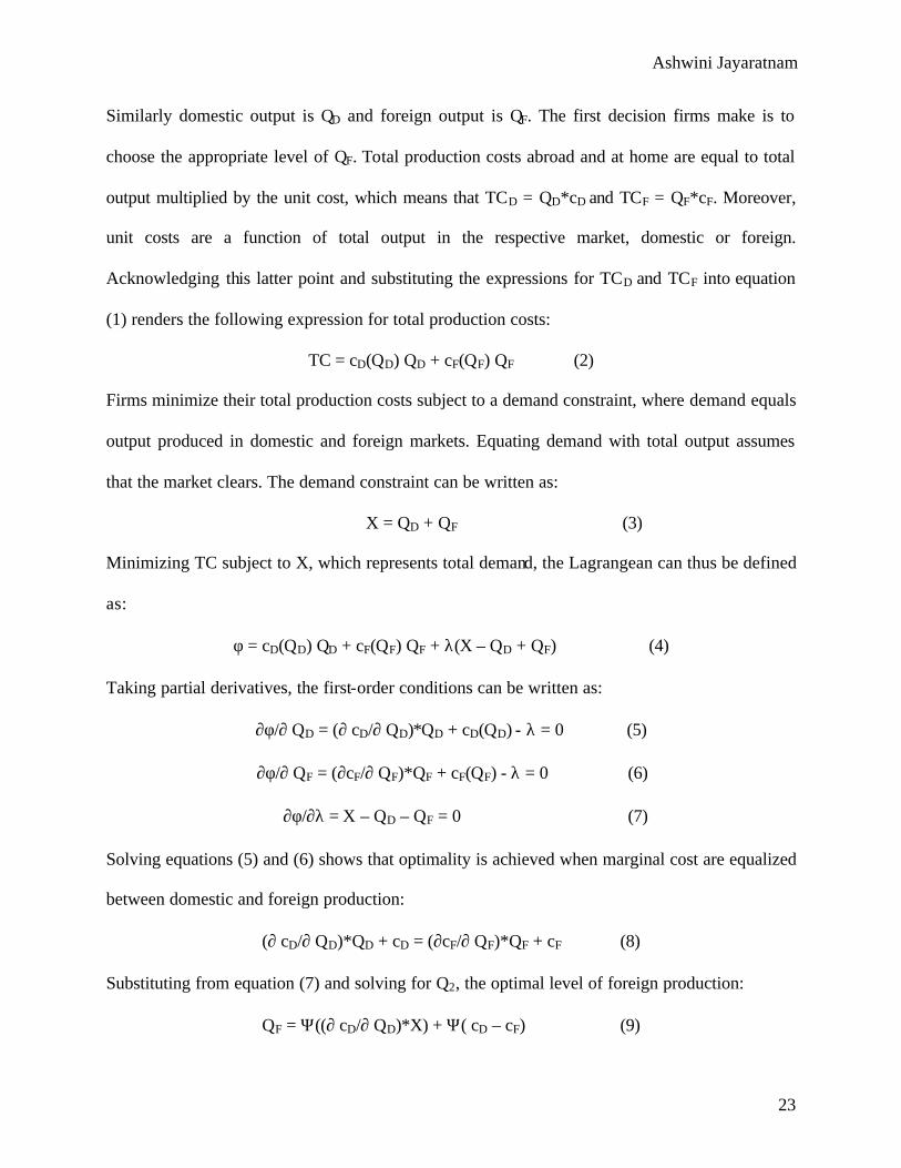
Similarly domestic output is QD and foreign output is QF. The first decision firms make is to

choose the appropriate level of QF. Total production costs abroad and at home are equal to total

output multiplied by the unit cost, which means that TCD = QD*cD and TCF = QF*cF. Moreover,

unit costs are a function of total output in the respective market, domestic or foreign.

Acknowledging this latter point and substituting the expressions for TCD and TCF into equation

(1) renders the following expression for total production costs:

TC = cD(QD) QD + cF(QF) QF (2)

Firms minimize their total production costs subject to a demand constraint, where demand equals

output produced in domestic and foreign markets. Equating demand with total output assumes

that the market clears. The demand constraint can be written as:

X = QD + QF (3)

Minimizing TC subject to X, which represents total demand, the Lagrangean can thus be defined

as:

φ = cD(QD) QD + cF(QF) QF + λ(X – QD + QF) (4)

Taking partial derivatives, the first-order conditions can be written as:

∂φ/∂ QD = (∂ cD/∂ QD)*QD + cD(QD) - λ = 0 (5)

∂φ/∂ QF = (∂cF/∂ QF)*QF + cF(QF) - λ = 0 (6)

∂φ/∂λ = X – QD – QF = 0 (7)

Solving equations (5) and (6) shows that optimality is achieved when marginal cost are equalized

between domestic and foreign production:

(∂ cD/∂ QD)*QD + cD = (∂cF/∂ QF)*QF + cF (8)

Substituting from equation (7) and solving for Q2, the optimal level of foreign production:

QF = Ψ((∂ cD/∂ QD)*X) + Ψ( cD – cF) (9)

Ashwini Jayaratnam

24

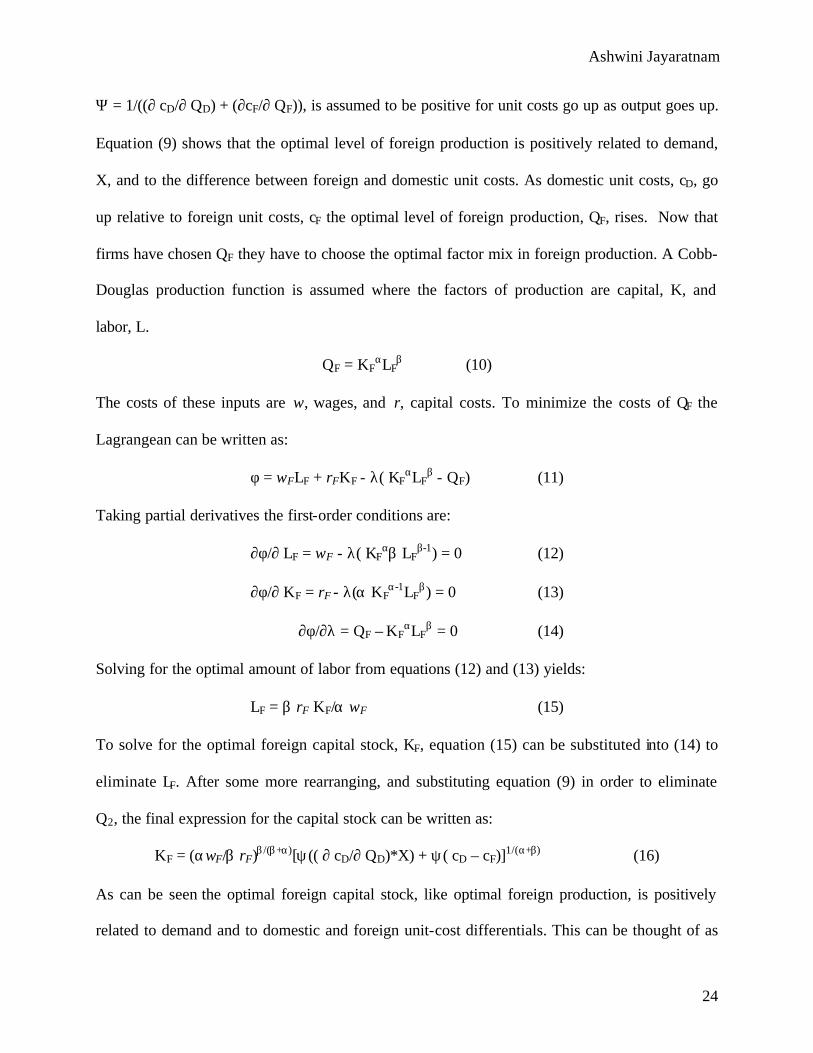
Ψ = 1/((∂ cD/∂ QD) + (∂cF/∂ QF)), is assumed to be positive for unit costs go up as output goes up.

Equation (9) shows that the optimal level of foreign production is positively related to demand,

X, and to the difference between foreign and domestic unit costs. As domestic unit costs, cD, go

up relative to foreign unit costs, cF the optimal level of foreign production, QF, rises. Now that

firms have chosen QF they have to choose the optimal factor mix in foreign production. A Cobb-

Douglas production function is assumed where the factors of production are capital, K, and

labor, L.

QF = KFαLF

β (10)

The costs of these inputs are w, wages, and r, capital costs. To minimize the costs of QF the

Lagrangean can be written as:

φ = wFLF + rFKF - λ( KFαLF

β - QF) (11)

Taking partial derivatives the first-order conditions are:

∂φ/∂ LF = wF - λ( KFαβ LF

β-1) = 0 (12)

∂φ/∂ KF = rF - λ(α KFα-1LF

β) = 0 (13)

∂φ/∂λ = QF – KFαLF

β = 0 (14)

Solving for the optimal amount of labor from equations (12) and (13) yields:

LF = β rF KF/α wF (15)

To solve for the optimal foreign capital stock, KF, equation (15) can be substituted into (14) to

eliminate LF. After some more rearranging, and substituting equation (9) in order to eliminate

Q2, the final expression for the capital stock can be written as:

KF = (αwF/β rF)β /(β+α)[ψ(( ∂ cD/∂ QD)*X) + ψ( cD – cF)]1/(α+β) (16)

As can be seen the optimal foreign capital stock, like optimal foreign production, is positively

related to demand and to domestic and foreign unit-cost differentials. This can be thought of as

Ashwini Jayaratnam

25

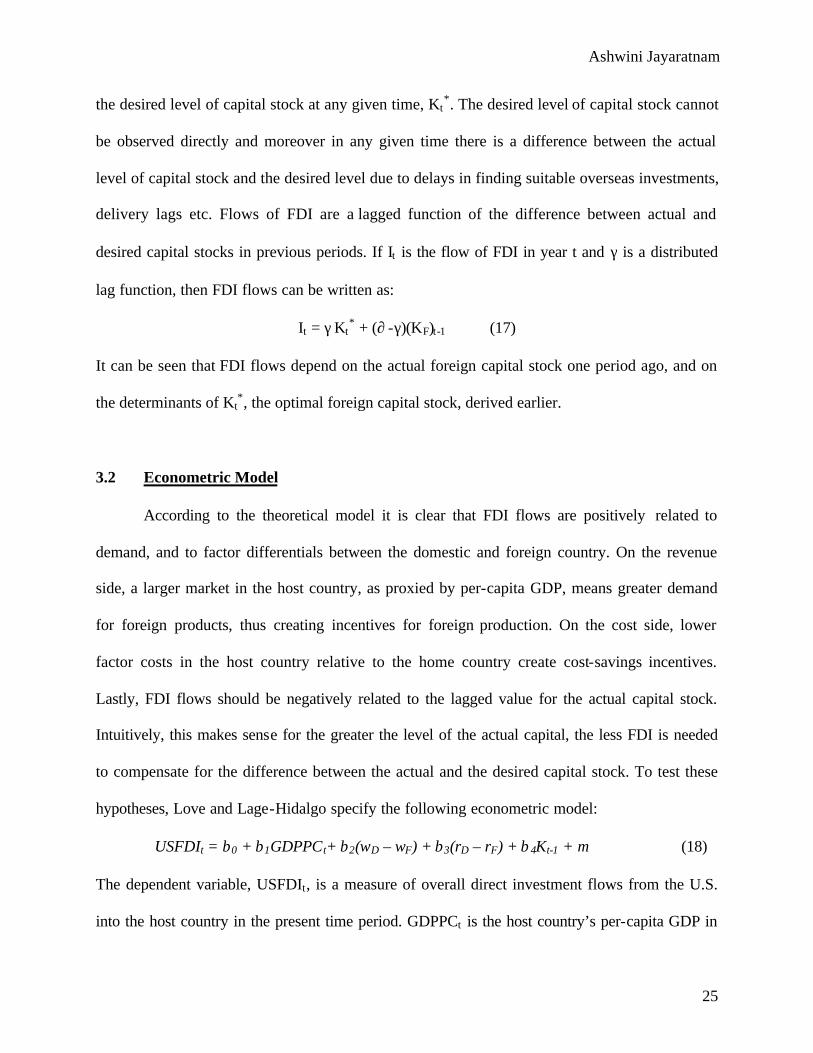
the desired level of capital stock at any given time, Kt*. The desired level of capital stock cannot

be observed directly and moreover in any given time there is a difference between the actual

level of capital stock and the desired level due to delays in finding suitable overseas investments,

delivery lags etc. Flows of FDI are a lagged function of the difference between actual and

desired capital stocks in previous periods. If It is the flow of FDI in year t and γ is a distributed

lag function, then FDI flows can be written as:

It = γ Kt* + (∂ -γ)(KF)t-1 (17)

It can be seen that FDI flows depend on the actual foreign capital stock one period ago, and on

the determinants of Kt*, the optimal foreign capital stock, derived earlier.

3.2 Econometric Model

According to the theoretical model it is clear that FDI flows are positively related to

demand, and to factor differentials between the domestic and foreign country. On the revenue

side, a larger market in the host country, as proxied by per-capita GDP, means greater demand

for foreign products, thus creating incentives for foreign production. On the cost side, lower

factor costs in the host country relative to the home country create cost-savings incentives.

Lastly, FDI flows should be negatively related to the lagged value for the actual capital stock.

Intuitively, this makes sense for the greater the level of the actual capital, the less FDI is needed

to compensate for the difference between the actual and the desired capital stock. To test these

hypotheses, Love and Lage-Hidalgo specify the following econometric model:

USFDIt = β0 + β1GDPPCt+ β2(wD – wF) + β3(rD – rF) + β4Kt-1 + µ (18)

The dependent variable, USFDIt, is a measure of overall direct investment flows from the U.S.

into the host country in the present time period. GDPPCt is the host country’s per-capita GDP in

Ashwini Jayaratnam

26

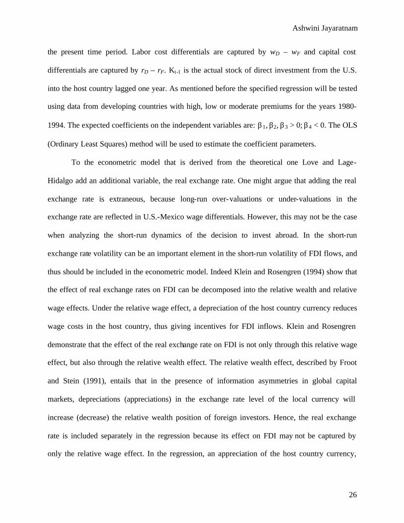
the present time period. Labor cost differentials are captured by wD – wF and capital cost

differentials are captured by rD – rF. Kt-1 is the actual stock of direct investment from the U.S.

into the host country lagged one year. As mentioned before the specified regression will be tested

using data from developing countries with high, low or moderate premiums for the years 1980-

1994. The expected coefficients on the independent variables are: β1, β2, β3 > 0; β4 < 0. The OLS

(Ordinary Least Squares) method will be used to estimate the coefficient parameters.

To the econometric model that is derived from the theoretical one Love and Lage-

Hidalgo add an additional variable, the real exchange rate. One might argue that adding the real

exchange rate is extraneous, because long-run over-valuations or under-valuations in the

exchange rate are reflected in U.S.-Mexico wage differentials. However, this may not be the case

when analyzing the short-run dynamics of the decision to invest abroad. In the short-run

exchange rate volatility can be an important element in the short-run volatility of FDI flows, and

thus should be included in the econometric model. Indeed Klein and Rosengren (1994) show that

the effect of real exchange rates on FDI can be decomposed into the relative wealth and relative

wage effects. Under the relative wage effect, a depreciation of the host country currency reduces

wage costs in the host country, thus giving incentives for FDI inflows. Klein and Rosengren

demonstrate that the effect of the real exchange rate on FDI is not only through this relative wage

effect, but also through the relative wealth effect. The relative wealth effect, described by Froot

and Stein (1991), entails that in the presence of information asymmetries in global capital

markets, depreciations (appreciations) in the exchange rate level of the local currency will

increase (decrease) the relative wealth position of foreign investors. Hence, the real exchange

rate is included separately in the regression because its effect on FDI may not be captured by

only the relative wage effect. In the regression, an appreciation of the host country currency,

Ashwini Jayaratnam

27

which in the Love and Lage-Hidalgo model is Mexico, relative to the home country currency, the

U.S. dollar, is predicted to negatively affect direct investment because the relative cost of

acquiring foreign assets rises. By symmetry, a highly depreciated host country exchange rate

reduces the cost of acquiring foreign assets, thus increasing FDI inflows.

However, in the regression, this result may be problematic to test, due to the real

exchange rate not being a truly exogenous variable. The real exchange rate is an endogenous

variable insofar as large capital inflows may push up the real exchange rate. C.H. Kwan (2001)

describes this phenomenon in regard to East Asian economies, whose real exchange rates are

extremely sensitive to volatile inflows and outflows of capital. Given that real exchange rates are

affected by capital flows, there is a simultaneity problem in the regression meaning tha t the

dependent variable, FDI inflows, has an effect on one of the independent variables. It may be

argued, however, that because FDI, unlike other types of capital flows, is undertaken over a

longer time horizon, in comparison to perhaps short-term portfolio flows, it does not bring as

much volatility to real exchange rates. However, the simultaneity problem could be important for

FDI as well, because foreign investors use foreign currency to buy domestic currency. If the

demand for domestic currency by foreign investors is significant, this will push up the host

country exchange rate. This effect is mitigated, however, to the extent that foreign companies

finance part of their operations from home country sources.

As a result of the simultaneity problem between FDI and real exchange rates, it is

difficult to ascertain the Froot and Stein result from the coefficient on the real exchange rate

variable. Going by the argument put forth by Froot and Stein, the coefficient on the real

exchange rate variable is expected to be positive, for as the real exchange rate depreciates

(increases) FDI inflows increase; by symmetry as the rate appreciates (decreases) FDI inflows

Ashwini Jayaratnam

28

decline. However, if FDI inflows push up real exchange rates, then there may be a downward

bias in the coefficient for the real exchange rate variable. A depreciated exchange rate should

bring in more FDI, but a depreciated exchange rate might in fact be the result of FDI outflows,

and thus the expected positive coefficient will have a downward bias.

This simultaneity problem may be explained away in the case of East Asian economies,

where one could claim that the real exchange rates, which are pegged to the dollar, are mostly

affected by changes in the yen-dollar rate as opposed to changes in total FDI inflows. This

hypothesis follows C.H. Kwan’s claim (2001) regarding the interdependence between East Asian

economies and the Japanese economy. Kwan claims that economic growth in Asia’s developing

countries is more affected by changes in the yen-dollar rate than by changes in the U.S. growth

rate. His empirical evidence to support this claim shows that a10 percent depreciation

(appreciation) of the yen against the dollar tends to drag down (push up) economic growth in

Asia’s developing countries by 1 percent. One of the channels through which the yen-dollar rate

affects Asian economies is through FDI from Japan. For instance, a depreciation of the yen

against the dollar reduces the cost of production in Japan relative to other Asian countries, and

thus there are fewer incentives for Japanese companies to relocate production to Asia, leading to

a decline in the inflow of FDI. By symmetry, an appreciation of the yen against the dollar, leads

to an increase in FDI inflows. As mentioned earlier, movements in FDI inflows affect real

exchange rates, and therefore movements in the yen-dollar rate, which affect Japanese FDI to

Asian developing countries, should affect real exchange rates in East Asia. Given the high degree

of interdependence between Japan and East Asia, it might be claimed that real exchange rates in

East Asia are not significantly affected by total FDI inflows, but rather by the yen-dollar rate and

FDI inflows from Japan. In this situation, it may not be too problematic to treat East Asian real

Ashwini Jayaratnam

29

exchange rates as exogenous. However, in the Love and Lage-Hidalgo study, the simultaneity

problem remains an issue, for one cannot say that Mexican real exchange rates are affected by

factors in a different economy as opposed to being affected by U.S. FDI inflows. Moreover, in a

study of several countries, one cannot rely on a similar situation as in East Asian economies.

My econometric model follows the one developed by Love and Lage-Hidalgo, and hence

I use GDP per-capita, labor and capital cost differentials, and real exchange rates as determinants

of the FDI. To these explanatory variables I will add the black market exchange premium. As

there have been no past studies on the effect of the black market exchange premium on FDI

flows, the sign on the coefficient for the black market premium is more difficult to predict. A

high black market exchange premium could mean that investors can acquire foreign assets at the

black market rate, and since the black market rate is depreciated compared to the official rate this

means that the price of foreign assets becomes relatively cheap. Of course this argument is based

on the assumption that governments do not force investors to go through the official market in

which case the depreciated black market rate won’t make any difference. The presence of a high

black market premium also implies that the official exchange rate is overvalued. According to

Froot and Stein (1991) an overvalued official exchange rate discourages foreign investment.

However, the existence of a black market for foreign exchange mitigates such an effect. The

result is that when the official exchange rate is overvalued, the coefficient on the black market

premium should be positive, for the black market encourages foreign investment by offering

investors the chance to acquire assets relatively cheaply.

A problem with using the black market premium and the real exchange rate in the same

regression is that these two explanatory variables are likely to be correlated. As said before, an

overvalued real exchange rate, gives rise to a high premium. Thus one is faced with the

Ashwini Jayaratnam

30

multicollinearity problem. To incorporate the black market premium into the regression and at

the same time avoid the multicollinearity problem, it would be best to run a preliminary

regression with the black market premium as the dependent variable and the real exchange rate

as the independent variable. This will reveal which part of the black market premium can be

explained by changes in the real exchange rate. However, instead of using the real exchange rate

as an explanatory variable in the preliminary regression, I use deviations of the real exchange

rate from purchasing power parity. Deviations of the real exchange rate render a better sense of

whether the exchange rate is overva lued or undervalued than the real exchange rate alone. The

regression of the black market premium on real exchange rate deviation is stated below:

Blk.Mkt.Prem = constant + B1RealExDeviation + u (19)

The residuals of regression (19) reveal that part of the black market premium that cannot be

explained by deviations in the real exchange rate. Hence, in my main regression I will use the

residuals of equation (19) as an explanatory variable. This captures the effect of the black market

premium, while averting the multicollinearity problem. I estimate the following model:

FDI = constant + B1GDPPC + B2Lab.Cost.Diff + B3Cap.Cost.Diff + B4RealExDeviation +

B5u + u2 (20)

The coefficient B5 is expected to be positive, because a high premium is predicted to mitigate the

effect of an overvalued exchange rate, thus stimulating FDI flows.

Ashwini Jayaratnam

31

4. Data Description

The dependent variable in the regression is net FDI inflows in millions of U.S. dollars.

The independent variables are: the black market premium, the real exchange rate deviation, per

capita GDP, labor cost differentials and real interest rate differentials. The time period is 1982-

1993 and 28 countries are included in the regression. These countries are listed in Table 1 (see

page 42).

Net FDI flows in U.S. dollars were obtained using balance of payments data for

individual countries from the World Bank’s World Development Indicators. Per capita GDP,

which serves as a proxy for demand in the host country, is also obtained from the World

Development Indicators and is measured in U.S. dollars.

Deviations from the real exchange rate are arrived at using Purchasing Power Parity

(PPP). Real exchange rate deviation is calculated as the percentage difference between the real

exchange rate at time t (which is somewhere between 1982 and 1993) and the average value of

the real exchange rate during that time period. Before calculating the deviation, it is necessary to

calculate the real exchange rate from the nominal exchange rate. The nominal exchange rate,

expressed in terms of foreign currency per US dollar and obtained from International Financial

Statistics, published by the IMF, is multiplied by the price level in the foreign country and

divided by the price level in the U.S. to get the real exchange rate. The real exchange rate is thus

expressed in terms of foreign currency per US dollar. The price levels in the foreign country and

the U.S. are proxied using the Consumer Price Index (CPI). It is often claimed that the CPI

overstates the level of inflation in comparison to other price indices such as the Wholesale Price

Index (WPI), which is an index of producer level prices of various commodities. Moreover, since

the WPI includes intermediate goods, not purchased by consumers, unlike the CPI, it is more

Ashwini Jayaratnam

32

weighted towards traded goods, which is important when studying foreign investment. However,

despite having certain advantages over the CPI, WPI data is frequently unavailable for

developing countries, and thus it is easier to use the CPI. Having used the CPI to calculate values

for the real exchange rate from 1982 to 1993, these values are averaged over that time period and

percentage deviations of the real exchange rate each year from the average value is taken to be

the real exchange rate deviation.

To calculate labor cost differentials I use data on real wage-manufacturing indices as

obtained from the ILO (International Labor Organization). Real wage indices are constructed by

dividing the index of average nominal wages by the CPI. The ILO reports wage rates for

countries in terms of the U.S. dollar, thus allowing for one to draw wage comparisons between

countries. While manufacturing wages certainly don’t account for all wages in a country, a vast

proportion of labor employed by multinational firms is in manufacturing and thus manufacturing

wages are an appropriate proxy for labor costs. The percentage difference between the real wage

manufacturing index for the host country and the U.S. real wage manufacturing index is used as

a measure of labor cost differentials. Real interest rate differentials between the host and home

country, which are a proxy for capital cost differentials, are measured as the percentage

difference between the U.S. real interest rate and the host country real interest rate. The real

interest rate will be the nominal rate, set by the Central Bank, minus the rate of inflation. To

measure the rate of inflation I use the percentage change in the CPI over one-year. This data is

obtained from International Financial Statistics, published by the IMF.

Finally, the black market premium is calculated in the same way as in past studies. Data

on the black market exchange rate was obtained from the Pick’s Currency Yearbook for the

years 1983-1988 and from Global Financial Statistics for the years 1989-1993. The premium is

Ashwini Jayaratnam

33

calculated as the percentage difference between the official exchange rate, obtained from the

IMF, and the black market exchange rate.

The mean, median, standard deviation and minimum and maximum values for the

independent and dependent variables are shown in Table 2 (see page 42). As can be seen several

of the variables vary significantly. This is particularly the case for the minimum and maximum

values of wage differentials, expressed as a percentage. The unusually high maximum value for

wage differentials can be attributed to extremely high labor costs in Israel in the early 1980s.

Other variables with significant outliers, as evidenced by the range of minimum and maximum

values in comparison to the mean and median, are the black market premium, real interest rate

differentials, and real exchange rate deviations. These variables also have large standard

deviations, which is a further indication of the presence of outliers in the data.

Table 3 (see page 42) shows correlations between the dependent and independent

variables and between certain independent variables. Regarding correlations between

independent variables, the ones that in theory should be significant include the correlation

between the black market premium and real exchange rate deviation, and the correlation between

real interest rate differentials and real exchange rate deviation. An over-valued real exchange

rate, meaning a large, negative deviation between the real exchange rate at time t and its average

value from 1982-1993, implies a high black market premium, and hence a positive correlation is

expected. A plot of the black market premium versus the real exchange rate deviation is shown

in Figure 1 (see page 43). However, as can be seen there does not appear to be a correlation

between the two variables. Regarding interest rate differentials, a higher real interest rate

differential between the host country and the U.S. interest rate should also mean that the host

country real exchange rate is less over-valued, and thus the deviation should be small. A plot of

Ashwini Jayaratnam

34

the real exchange rate deviation versus real interest rate differentials can be found in Figure 2

(see page 44). Yet here again, there appears to be no correlation.

5. Analysis of Econometric Results (1) Blk.Mkt.Prem = constant + B1RealExDeviation + u

The purpose of running regression (1) is to test the collinearity between two independent

variables that will be used in the main regression: the black market exchange premium and the

deviation of the real exchange rate from its value under purchasing power parity (PPP). The

regression tests to what extent the black market premium might be explained by an overvalued or

undervalued real exchange rate. The residuals of the regression constitute that part of the black

market premium that is unexplained by overvaluations or undervaluations of the real exchange

rate. Hence, the residuals will be used as an additional explanatory variable in the main

regression. Using the residuals of this regression incorporates the black market premium into the

main regression, while averting the multicollinearity problem. The results of regression (1) are

summarized below:

Coef. Std. Err. t

B1 -.43 .214 -2.02 cons 84 18.2 4.60 R-squared = 0.0151 Adj R-squared = 0.0114

In regression (1) above both the black market premium and real exchange rate deviations are

expressed as percentages. The sign on the coefficient for the real exchange rate devia tion is as

predicted. A 1 percentage point increase in the deviation from PPP, meaning that the real

exchange rate becomes more devalued compared to its average value under purchasing power

Ashwini Jayaratnam

35

parity, leads to a 0.43 percentage point decline in the black market premium. This is fitting with

the hypothesis that an overvalued real exchange rate, which would mean that the deviation goes

down relative to its average value under purchasing power parity, leads to an increase in the

premium. The reasoning behind this hypothesis is that an overvalued real exchange rate creates

an excess demand for foreign exchange, which cannot be satisfied under the official rate system.

As a result, the black market rate for foreign currency goes up creating a high black market

premium. Conversely an undervalued real exchange rate leads to a decrease in the premium. The

absolute value of the t-statistic on the real exchange rate deviation coefficient, 2.02, reveals that

it is significant at the 5% level.

When there is no deviation in the real exchange rate, the average value of the black market

premium among the sample of countries studies is 84%. This is the value of the constant, whose

t-statistic is 4.60, showing a high level of significance.

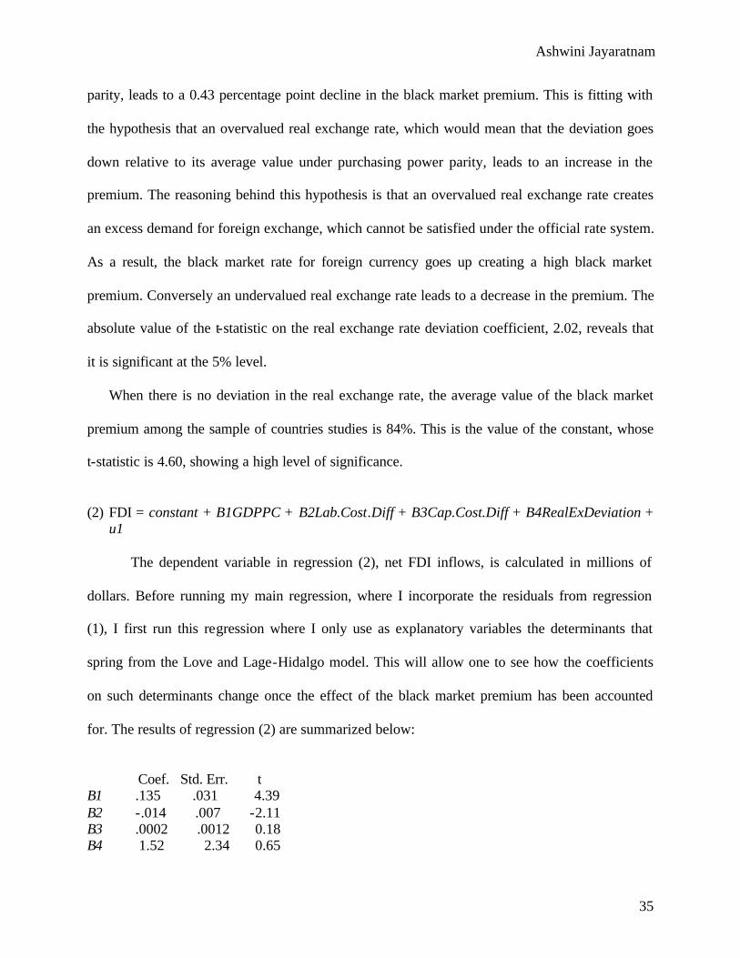
(2) FDI = constant + B1GDPPC + B2Lab.Cost.Diff + B3Cap.Cost.Diff + B4RealExDeviation +

u1

The dependent variable in regression (2), net FDI inflows, is calculated in millions of

dollars. Before running my main regression, where I incorporate the residuals from regression

(1), I first run this regression where I only use as explanatory variables the determinants that

spring from the Love and Lage-Hidalgo model. This will allow one to see how the coefficients

on such determinants change once the effect of the black market premium has been accounted

for. The results of regression (2) are summarized below:

Coef. Std. Err. t

B1 .135 .031 4.39 B2 -.014 .007 -2.11 B3 .0002 .0012 0.18 B4 1.52 2.34 0.65

Ashwini Jayaratnam

36

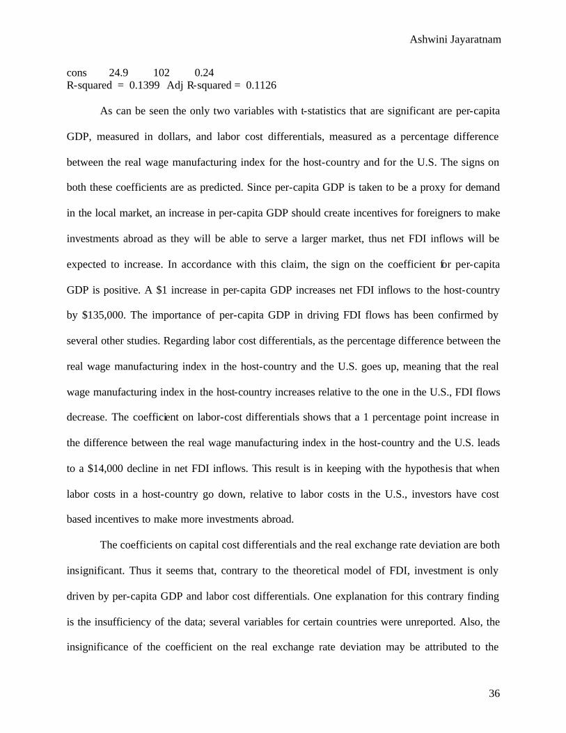
cons 24.9 102 0.24 R-squared = 0.1399 Adj R-squared = 0.1126

As can be seen the only two variables with t-statistics that are significant are per-capita

GDP, measured in dollars, and labor cost differentials, measured as a percentage difference

between the real wage manufacturing index for the host-country and for the U.S. The signs on

both these coefficients are as predicted. Since per-capita GDP is taken to be a proxy for demand

in the local market, an increase in per-capita GDP should create incentives for foreigners to make

investments abroad as they will be able to serve a larger market, thus net FDI inflows will be

expected to increase. In accordance with this claim, the sign on the coefficient for per-capita

GDP is positive. A $1 increase in per-capita GDP increases net FDI inflows to the host-country

by $135,000. The importance of per-capita GDP in driving FDI flows has been confirmed by

several other studies. Regarding labor cost differentials, as the percentage difference between the

real wage manufacturing index in the host-country and the U.S. goes up, meaning that the real

wage manufacturing index in the host-country increases relative to the one in the U.S., FDI flows

decrease. The coefficient on labor-cost differentials shows that a 1 percentage point increase in

the difference between the real wage manufacturing index in the host-country and the U.S. leads

to a $14,000 decline in net FDI inflows. This result is in keeping with the hypothesis that when

labor costs in a host-country go down, relative to labor costs in the U.S., investors have cost

based incentives to make more investments abroad.

The coefficients on capital cost differentials and the real exchange rate deviation are both

insignificant. Thus it seems that, contrary to the theoretical model of FDI, investment is only

driven by per-capita GDP and labor cost differentials. One explanation for this contrary finding

is the insufficiency of the data; several variables for certain countries were unreported. Also, the

insignificance of the coefficient on the real exchange rate deviation may be attributed to the

Ashwini Jayaratnam

37

downward bias on the coefficient due to the endogeneity between real exchange rates and FDI

inflows that was described earlier. With regard to capital costs being insignificant it could be that

the measure chosen to proxy capital cost differentials, namely real interest rate differentials

between the host-country and the U.S., was inappropriate. Instead of only using interest rates to

measure capital costs, Love and Hidalgo (2000), in their regression, also use the gross capital

formation deflator. However, data on this indicator is largely unavailable for developing

countries. The problem with using real interest differentials alone is that they are may be

correlated with the real exchange rate in the host-country, which is believed to affect FDI flows.

However, since the coefficient on real interest rate differentials is neither statistically or

economically significant, any bias in the coefficient need not be considered. A further

explanation for the lack of significance of the coefficients for the real interest rate differential

and the real exchange rate deviation is perhaps the sample of countries used. Several of the

countries with black markets for foreign exchange also have relatively low labor costs; some

examples are Malaysia and Indonesia. As a result, it might be the case that low labor costs are

key drivers of FDI to these countries as opposed to considerations of capital costs or exchange

rate deviation. Perhaps in a larger sample of countries, these other factors will be significant.

(3) FDI = constant + B1GDPPC + B2Lab.Cost.Diff + B3Cap.Cost.Diff + B4RealExDeviation +

B5u + u2

In regression (3), I include the residuals, u, from regression (1). These residuals represent

the part of the black market premium that is unrelated to deviation in the real exchange rate from

PPP. The coefficient on u is expected to be positive as a depreciated black market rate, indicated

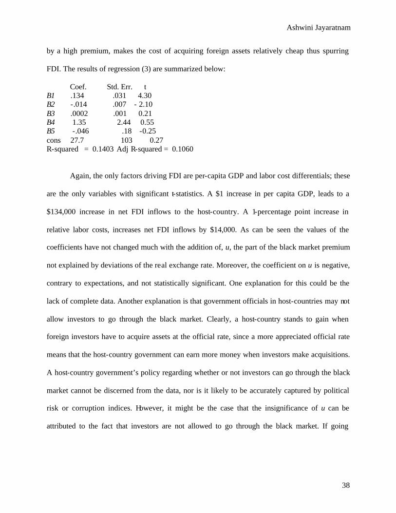
Ashwini Jayaratnam

38

by a high premium, makes the cost of acquiring foreign assets relatively cheap thus spurring

FDI. The results of regression (3) are summarized below:

Coef. Std. Err. t B1 .134 .031 4.30 B2 -.014 .007 - 2.10 B3 .0002 .001 0.21 B4 1.35 2.44 0.55 B5 -.046 .18 -0.25 cons 27.7 103 0.27 R-squared = 0.1403 Adj R-squared = 0.1060

Again, the only factors driving FDI are per-capita GDP and labor cost differentials; these

are the only variables with significant t-statistics. A $1 increase in per capita GDP, leads to a

$134,000 increase in net FDI inflows to the host-country. A 1-percentage point increase in

relative labor costs, increases net FDI inflows by $14,000. As can be seen the values of the

coefficients have not changed much with the addition of, u, the part of the black market premium

not explained by deviations of the real exchange rate. Moreover, the coefficient on u is negative,

contrary to expectations, and not statistically significant. One explanation for this could be the

lack of complete data. Another explanation is that government officials in host-countries may not

allow investors to go through the black market. Clearly, a host-country stands to gain when

foreign investors have to acquire assets at the official rate, since a more appreciated official rate

means that the host-country government can earn more money when investors make acquisitions.

A host-country government’s policy regarding whether or not investors can go through the black

market cannot be discerned from the data, nor is it likely to be accurately captured by political

risk or corruption indices. However, it might be the case that the insignificance of u can be

attributed to the fact that investors are not allowed to go through the black market. If going

Ashwini Jayaratnam

39

through the black market is not an option for foreign investors, they will not consider it an

important factor when making investment decisions.

A further explanation may be found by going back to the theoretical basis for why the

black market premium was thought to have a positive effect. The claim that the black market

premium serves to mitigate the effect of an overvalued real exchange rate thus stimulating

foreign investment follows the argument of Froot and Stein (1991). This argument is premised

on the claim that an overvalued exchange rate increases the relative cost of acquiring foreign

assets. However, Campa (1993) puts forth an opposite claim that an overvalued exchange rate in

the host-country should encourage foreign investment, for this increases a firm’s expectations of

future profitability in terms of the home currency. Thus it might be argued that a large premium

deters FDI, because investors have to convert their profits into the home currency at the black

market rate, which is depreciated compared to the official rate. This argument is in line with the

negative coefficient on u. However, it does not explain the fact that the coefficient is

insignificant.

6. Conclusions

From the results it can be seen that, contrary to hypothesis, the black market exchange

premium does not affect net FDI inflows. Some of the reasons for this contrary result were

discussed in the previous section. However, if this result is in fact accurate, then liberalization of

currency regimes in developing countries, which leads to the disappearance of black markets,

should not be expected to bring in more or less foreign investment, the reason being that the

black market premium did not in the past impede nor enhance foreign investment.

Ashwini Jayaratnam

40

Looking at the other results from my regression, some conclusions regarding the

determinants of FDI to developing countrie s may be drawn. It appears that per-capita GDP and

wage differentials are the key drivers of FDI to developing countries. Such a result is in line with

the conclusions of past studies on the determinants of FDI. Firms are drawn to host-countries

with a large market size, proxied by GDP or GDP per-capita, where demand for their product is

expected to be high. This is often referred to as the market seeking hypothesis, under which firms

look for host-countries where they can easily market and sell their products. The importance of a

growing economy, indicative of a large market, in attracting FDI can be a somewhat problematic

notion to the extent that FDI itself is necessary for the growth of developing countries. Firms in

industrialized countries may not be attracted to investing in host-countries with low GDP growth

rates. As a result, such countries will be further impeded in their attempts to grow the economy,

as they do not get the many benefits of foreign investment. Regarding labor-cost differentials,

past studies have also shown low labor-costs to be key drivers of FDI. Firms relocate abroad in

order to take advantage of cheap labor, as well as other raw materials costs.

In fact, the impetus behind Love and Hidalgo’s (2000) study of the determinants of U.S.

foreign investment to Mexico, from which I developed my own model, was to examine how

much of the increase in FDI through time could be attributed to the cheap labor effect and how

much to the size of the Mexican market. The cheap labor effect was thought to be boosted by the

maquiladora industrialization program, where the Mexican government removed tariffs on

imports in order to attract multinational enterprises to the maquiladora industry where they could

take advantage of the cheap labor. However, the growth of the Mexican economy between 1967

and 1994, a large part of which in fact resulted from the increase in employment in the

Ashwini Jayaratnam

41

maquiladora sector as multinational firms relocated production, was also thought to be a

determinant of increased net FDI inflows.

Having discussed the significance of market size and labor-cost differentials, and the

insignificance of the black market premium in explaining FDI to developing countries, some

further areas of research in studying the determinants of foreign investment might be pointed out.

Recently, the importance of a country’s institutional framework is being recognized. Accounting

for institutional considerations includes factoring in the effects of economic and political

instability on the business climate. Indeed economic and political instability are often claimed to

be correlated with the black market premium. A high premium is indicative of high economic

and financial instability in a country, as would be expected since a high premium signals an

overvalued official exchange rate. Also, a high black market premium is said to be correlated

with political instability. Due to correlations with political and economic instability, the black

market premium might in fact have a negative effect on foreign investment, contrary to the

positive effect that I predicted on the grounds that it mitigates the effect of an overvalued

exchange rate. It should be noted that quantifying institutional variables such as political

instability is problematic and subject to bias. Several political risk indices, which factor in

corruption, property rights, rule of law, and political violence, are believed to be subjective in

their weighing of factors that constitute political instability. Nonetheless, taking into account a

country’s institutional framework might yield a better understanding of whether or not the black

market premium in fact affects FDI, for black markets and political and economic instability are

thought to be correlated.

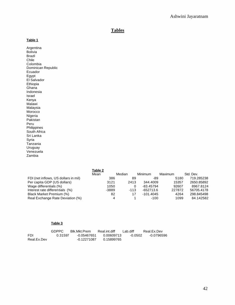
Ashwini Jayaratnam

42

Tables

Table 1

Argentina Bolivia Brazil Chile Colombia Dominican Republic Ecuador Egypt El Salvador Ethiopia Ghana Indonesia Israel Kenya Malawi Malaysia Morocco Nigeria Pakistan Peru Philippines South Africa Sri Lanka Syria Tanzania Uruguay Venezuela Zambia

Table 2 Mean Median Minimum Maximum Std. Dev.

FDI (net inflows, US dollars in mil) 386 89 -89 5180 719.285238 Per capita GDP (US dollars) 3121 2413 344.4009 15357 2650.85892 Wage differentials (%) 1050 0 -83.45794 92607 8967.8124 Interest rate differentials (%) -3889 -113 -652713.6 227872 56705.4178 Black Market Premium (%) 82 17 -101.4045 4264 298.845498 Real Exchange Rate Deviation (%) 4 1 -100 1099 84.142582

Table 3 GDPPC Blk.Mkt.Prem Real.int.diff Lab.diff Real.Ex.Dev

FDI 0.31597 -0.05467651 0.00609713 -0.0502 -0.0796596 Real.Ex.Dev -0.12271087 0.15899765

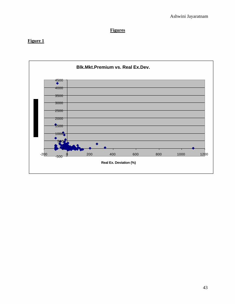
Ashwini Jayaratnam

43

Figures

Figure 1

Blk.Mkt.Premium vs. Real Ex.Dev.

-500

0

500

1000

1500

2000

2500

3000

3500

4000

4500

-200 0 200 400 600 800 1000 1200

Real Ex. Deviation (%)

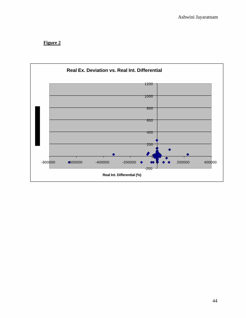
Ashwini Jayaratnam

44

Figure 2

Real Ex. Deviation vs. Real Int. Differential

-200

0

200

400

600

800

1000

1200

-800000 -600000 -400000 -200000 0 200000 400000

Real Int. Differential (%)

Ashwini Jayaratnam

45

References

Aizenman, Joshua. 1994. “Monetary and Real Shocks, Productive Capacity and Exchange Rate Regimes.” Economica 61:407-34. Amuedo-Dorantes, Catalina and Susan Pozo. 2001. “Foreign Exchange Rates and Foreign Direct Investment in the United States.” International Trade Journal 15:323-43. Asiedu, Elizabeth. 2002. “On the Determinants of Foreign Direct Investment to

Developing Countries: Is Africa Different?” World Development 30:107-19.

Barrell, Ray and Nigel Pain. 1996. “An Econometric Model of U.S. Foreign Direct Investment.” The Review of Economics and Statistics 78:200-7.

Biswas, Romita. 2002. “Determinants of Foreign Direct Investment.” Review of Development Economics 6:492-504.

Blonigen, Bruce A. 1997. “Firm Specific Assets and the Link Between Exchange Rates and Foreign Direct Investment.” American Economic Review 87:447-65.

Calvo, G.A., L. Leiderman and C.M. Reinhart. 1993. “Capital Inflows and Real Exchange Rate

Appreciation in Latin America.” IMF Staff Papers 40:108-115. Campa, J.M. 1993. “Entry by Foreign Firms in the United States under Exchange Rate

Uncertainty.” Review of Economics and Statistics 75:614-22. Cushman, D.O. 1987. “The Effects of Real Wages and Labor Productivity on Foreign Direct

Investment.” Southern Economic Journal 54:175-85. Cushman, D.O. 1985. “Real Exchange Rate Risk, Expectations and the Level of Direct

Investment.” Review of Economics and Statistics 67:297-308. Dornbusch, Rudiger, Daniel V. Dantas, Clarice Pechman, Roberto de Rezende Rocha and

Demetrio Simoes. 1983. “The Black Market for Dollars in Brazil.” NBER Reprint 364, 25-40.

Edwards, Sebastian. 1989. Real Exchange Rates, Devaluation and Adjustment: Exchange Rate

Policy in Developing Countries. MIT Press, Cambridge, Massachusetts. Froot, K and J. Stein. 1991. “Exchange Rates and Foreign Direct Investment: An Imperfect

Capital Markets Approach.” Quarterly Journal of Economics 196:1191-218. Goldberg, L.S. and C.D. Kolstad. 1995. “Foreign Direct Investment, Exchange Rate Variability

and Demand Uncertainty.” International Economic Review 36:855-73.

Ashwini Jayaratnam

46

Gorg, Holger and Katherine Wakelin. 2002. “The Impact of Exchange Rate Volatility on US

Direct Investment.” Manchester School 70:380-97. Kiguel, Miguel A, J. Saul Lizondo and Stephen A. O’Connell. 1997. Parallel Exchange Rates in

Developing Countries. Ipswich, Great Britain. Klein, M.W. and E. Rosengren. 1994. “The Real Exchange Rate and Foreign Direct Investment

in the United States: Relative Wealth vs. Relative Wage Effects.” Journal of International Economics 36:373-89

Kugler, Maurice. 2001. The Diffusion of Externalities From Foreign Direct Investment: Theory

Ahead of Measurement. Cambridge University Press. Kwan, C.H. 2001. “Deepening Japan-Asia Interdependence.” In Yen Block: Toward Economic

Integration in Asia, 38-61. Washington: Brookings Institution Press. Love, James H. and Francisco Lage-Hidalgo. 2000. “Analyzing the Determinants of US Direct

Investment in Mexico.” Applied Economics 32:1259-67. Saca, Nolvia N. 1997. Black Market Exchange Rate, Unification of the Foreign Exchange

Markets and Monetary Policy: The Case of El Salvador. Peter Lang. Sercu, P and C. Vanhulle. 1992. “Exchange Rate Volatility, International Trade and the Value of

Exporting Firms.” Journal of Banking and Finance 16:55-182.