Housing and the Journey to Work in U.S. Cities · 6 Housing and the Journey to Work in U.S. Cities...

This PDF is a selection from an out-of-print volume from the National Bureauof Economic Research

Volume Title: Housing Markets in the U.S. and Japan

Volume Author/Editor: Yukio Noguchi and James Poterba

Volume Publisher: University of Chicago Press

Volume ISBN: 0-226-59015-1

Volume URL: http://www.nber.org/books/nogu94-2

Conference Date: January 3-4, 1991

Publication Date: January 1994

Chapter Title: Housing and the Journey to Work in U.S. Cities

Chapter Author: Michelle J. White

Chapter URL: http://www.nber.org/chapters/c8824

Chapter pages in book: (p. 133 - 160)

6 Housing and the Journey to Work in U.S. Cities Michelle J. White

6.1 Introduction

This paper explores how the urban environment in the United States shapes the pattern of housing development. I focus on three major trends. First, during the postwar period, both housing and jobs in U.S. cities have suburbanized rapidly. As a result, U.S. cities have become very spread out and cover a great deal of land. New development on the fringes occurs at very low density levels. Second, urban commuters in the United States have shifted from commuting by public transportation to commuting by automobile. I argue that these two trends are closely related and self-reinforcing: automobile commuting enabled jobs to suburbanize, but once they had suburbanized, more and more jobs were accessible only by car. Third, higher-income households generally choose to live farther from the city center than lower-income households. This phenomenon was true in the past and continues to be true in US. cities. Since higher- income households in the United States tend to choose suburban rather than central locations in cities, their behavior reinforces the trend for cities to suburbanize. This paper documents these trends in U.S. housing development and attempts to explain them.

A few basic facts concerning U.S. cities should be noted. The downtown area, usually the historic center, of U.S. cities is referred to as the central business district, or CBD. CBDs consist of concentrated office/employment dis- tricts with few residents, which have the highest density levels in their metropolitan areas and are surrounded by residential areas. Other employment subcenters, less dense than the CBD, are scattered around the metropolitan

Michelle J. White is professor of economics at the University of Michigan. The author is grateful to Sharon Parrott for very capable research assistance and to Charles Lave

for helpful comments.

133

134 Michelle J. White

area. They are often located at major road or public transportation intersections in both the central city and suburbs. The political structure of U S . metropolitan areas consists of a central city and many small suburban jurisdictions, each of which is a separate local government. There may be from ten to several hundred independent suburban jurisdictions. The central city and the suburban jurisdictions each provide public services such as education, police and fire protection, streets, trash collection, and some social services. In a typical metropolitan area, the central city contains one-third to one-half the entire metropolitan-area population and the suburban jurisdictions contain the rest.

Section 6.2 reviews the major economic theories of urban spatial structure and explores their implications for urban housing. Section 6.3 provides data illustrating the changes in the metropolitan housing stock in the United States during the postwar period. Section 6.4 explores the spatial pattern of employment in cities and its implications for how workers’ job locations and their residences are related by the commuting journey. Section 6.5 is the conclusion.

6.2 Population Growth and Suburbanization in U.S. Cities

Economists analyzing urban housing patterns have focused on explaining three broad trends: first, how rising real incomes over time have affected the spatial pattern of housing development; second, how falling costs of commuting in cities affect the spatial pattern of housing; and third, how high- versus low-income households differ in their taste for housing consumption in cities.

Two approaches have dominated economists’ thinking. The first is the Mills- Muth urban spatial model and the second is a historical model of urban growth. I also explore a variety of other factors that do not fit neatly into either model. It should be noted that most of the models described in this section assume that all jobs in cities are located at the CBD and that each household has one worker only.

6.2.1 The Mills-Muth Model of Urban Development

The Mills-Muth model, in its simplest form, assumes that all households have identical tastes and incomes and each has one worker. Households maximize utility over consumption of housing and a composite other good. Com- muting to work is costly, so that a worker’s income minus commuting cost must equal the household’s expenditure on housing and the composite good. Locational equilibrium in the metropolitan area requires that all households achieve the same utility level living at any location in the city, since otherwise households would move to the locations where utility is highest and housing prices would readjust. Based on these assumptions, it can be shown that the per unit price of land is highest near the CBD-where land is most scarce- and falls at a diminishing rate with distance from the CBD. This is because commuting cost increases with distance, requiring that the price of land fall in order to make households indifferent to commuting farther. By itself, this ef-

135 Housing and the Journey to Work in U.S. Cities

fect explains why land prices fall at a constant rate with distance from the CBD. But as land prices fall relative to the cost of other goods, households shift toward consuming more land and less other goods. This shift toward greater land consumption reduces the rate of decrease of land prices-hence land prices overall fall at a diminishing rate with distance.' Small, high-density housing units (apartments) are built near the CBD, where the price of land is high, and large, low-density housing units (single-family houses) are built in the suburbs, where the price of land is low. Households living near the CBD consume less housing but have more money available for consumption of other goods; while households living farther away from the CBD consume more housing and less other goods.

As a summary measure characterizing the spatial pattern of housing in cities, economists have estimated density/distance functions. It is straightfor- ward to show in the Mills-Muth model that population density, housing density, land prices, and housing prices must all decline at a decreasing rate with distance from the CBD. Since there is no reliable source-of data on land prices in U.S. cities, urban economists have concentrated on estimating density/distance functions rather than land price/distance functions. The density/distance relationship is usually represented as a negative exponential function. The critical parameter of this function, referred to as the density gradient, gives the propor- tional rate of decrease in density per mile of increase in distance from the CBD. In the next section, I present the results of estimating population density/ distance functions for a sample of U.S. cities. These have the advantage of being available over a fairly long span of time.'

Over time, two major trends have occurred in U.S. cities: faster modes of commuting have been introduced and household incomes have risen. Commut- ing costs include both time costs and out-of-pocket costs. The introduction of faster commuting modes lowers the time required to commute a mile and, since most of the cost of commuting is time cost, lowers the total cost of commuting per mile. A decline in the cost of commuting per mile causes the density/distance function to flatten, so that the density gradient approaches zero. This is because the scarce land near the CBD is no longer as valuable, since it is now cheaper to commute to the CBD from farther away. Conversely, the more plentiful land in the suburbs becomes more valuable, since it is

1. The price of land or housing as a function of distance from the CBD is denoted R(x), where x is distance from the CBD. It can be shown that R(x) must satisfy the following condition: dR(x)/dx = - f /h(x) , where f is the cost of commuting per mile round trip and h(x) is housing demand. Since h(x) rises as distance increases, R(x) declines at a diminishing rate with distance.

2. The negative exponential function is D(x) = D,e-Y", where D(x) is the number of people or the number of housing units per square mile of land x miles from the CBD, Do is the number of people or housing units per unit of land area at the CBD, and -y is the density gradient or the rate of decline in population or housing density per mile increase in distance from the CBD. Note that use of the negative exponential density function ignores the fact that population and housing densities are very low near the CBD, since business rather than residential land use predominates there.


cheaper to commute from the suburbs to the CBD. As a result, housing densities in the suburbs rise relative to housing densities near the CBD. Also, the city increases in size, since agricultural land at the outer periphery is converted to urban use.

An increase in household income has two offsetting effects on the density/ distance function. First, as household income rises, households demand more housing and/or higher-quality housing. Land is a component of housing and is cheaper in the suburbs, so higher-income households find the suburbs relatively more attractive, since the cost of housing per unit is lower there. Second, higher income causes the value of time spent commuting to rise, which makes housing near the CBD more attractive. If the income elasticity of housing demand exceeds the income elasticity of the value of time spent commuting, then an increase in household income causes the densityldistance function to flatten.3 Assuming that this condition holds, then the two important time trends in metropolitan areas both cause the density/distance function to flatten.4

The model can also be extended to include more than one income class. Suppose there are two income groups and the income elasticity of housing demand exceeds the income elasticity of the value of time spent commuting. Then lower-income households will occupy housing located in an inner ring around the CBD, and higher-income households will occupy housing located in an outer ring around the low-income households. Intuitively, this means that the suburbs’ low housing price attracts higher-income households more than the high cost of commuting repels them.5 Paradoxically, low-income households occupy high-priced land, although they consume relatively little of it by living in high-density housing, while high-income households occupy lower- priced land.

6.2.2

Now turn to the historical model of urban development, first proposed by Harrison and Kain (1974). It is based on the idea that cities originate at arbi-

The Historical Model of Urban Development

3. Differentiating dR(x)/dx with respect to income, we get

where Y denotes household income, E~ is the income elasticity of demand for housing, and E” is the income elasticity of the value of time spent commuting. The rent function becomes flatter as income increases if this expression is positive, which requires that E~ > E,

4. Whether in fact the income elasticity of housing demand exceeds the income elasticity of the value of time spent commuting is unclear. If the value of time spent commuting is a constant fraction of the hourly wage rate, as many studies have assumed (McFadden 1974), then the income elasticity of time spent commuting is unity. But Polinsky and Ellwood (1979) argue that the income elasticity of housing demand is less than unity.

5 . This short summary neglects a number of extensions of the Mills-Muth model, such as a dynamic version (Wheaton 1982), version in which some households have two workers, and ver- sions in which there are two or more taste classes. See below for discussion of the model when firms are assumed to locate outside the CBD.


trary locations determined by historical considerations-usually at a port or rail junction-and then expand outward over time from their historic centers. In the Mills-Muth model, whenever exogenous changes occur, the city’s housing stock is assumed to be completely rebuilt to reflect the new conditions. In contrast, the historical model assumes that housing is infinitely durable, so that once built, it remains unchanged. Therefore cities consists of inner rings of older housing around the CBD and outer rings of newer housing in the suburbs. The newest housing is always on the periphery of the city. The gradual introduction of faster commuting modes is also an important element in the historical model, since as commuting speeds rise and commuting costs fall, workers can live farther away from the CBD without increasing their commuting costs. Therefore when a faster commuting mode is introduced, the city expands by adding a new ring of housing on the periphery, since workers are willing to live farther away from the CBD. Faster commuting thus allows cities to increase in both population and area.

Since the early nineteenth century, when the dominant mode of commuting was walking, there have been a number of changes in commuting mode. Horse- drawn wagons were the first public transportation system, followed by steam- powered vehicles, underground rail systems, electric-powered streetcars, and motorized buses running on surface roads. In general, new public transportation modes were faster than their predecessors, and each new mode led to new housing built at the periphery, which was occupied by commuters. In the postwar period, commuting by automobile has largely replaced commuting by public transportation, which has dramatically increased commuting speeds and enabled cities to increase greatly in land area.

New commuting modes tended to be faster and more expensive in terms of out-of-pocket costs than their predecessors-at least initially. This means that for high-income workers, the total cost of the new commuting mode is cheaper than the total cost of older modes of commuting, since their value of time is high. But for low-income workers, the total cost of the new commuting mode is more expensive, since their value of time is lower. Therefore, the earliest group of users of new commuting modes tends to be high-income workers. But if high-income workers shift to the new mode and low-income workers continue using the older mode, then high-income workers at least temporarily have lower commuting costs per mile than low-income workers. As a result, high-income housing is built on the periphery of the city and occupied by high- income workers who use the fast commuting mode and can therefore commute farther. Low-income workers remain in older housing closer to the CBD. Later, the fast commuting mode falls in price and is adopted by all workers, which might suggest that spatial income segregation would be eroded. But by this time, new suburban rings have already been developed with high-income housing. Thus an alternative explanation of why we observe high-income housing in the suburbs is that high-income workers adopt faster commuting modes earlier and thus have a lower marginal cost of commuting than low-income work-


ers. This explanation suggests that a pattern of high-income households living in the suburbs and low-income households living near the CBD might be observed even if the income elasticity of housing demand were smaller than the income elasticity of the value of time spent commuting6

The introduction of the automobile for commuting differs from prior mode shifts, since it replaced commuting by public transportation witk commuting by private transportation. Compared to public transportation, the automobile involves a very low time cost per mile since it is much faster than commuting by bus or train. This might suggest that it would be adopted for commuting by workers of all income levels at the same time. The automobile also involves a high fixed cost, however-the cost of purchase. So high-income workers still adopted it earlier than low-income workers.

Another important aspect of the historical model is that housing units fall in quality as they age. This is both because older houses gradually wear out, which increases maintenance costs, and because older houses become economically obsolete, since they do not contain modem features such as air con- ditioning, insulation, multiple bathrooms, and modern kitchens. Higher- income households demand higher-quality housing than lower-income households (as well as more housing). Higher-quality housing tends to be cheaper to provide in the suburbs, where the housing stock is newer. In contrast, to provide high-quality housing near the CBD, old houses must be renovated or replaced, which is very expensive. Thus as housing ages and its quality falls, high-income households move from older housing nearer the CBD to newer housing farther out. The older housing vacated by high-income households is occupied by middle-income households, whose housing in turn is occupied by lower-income households in a process known as filtering. Thus over time, individual housing units move down the income scale. Filtering has the effect of reducing the amount of new housing built for middle- and low-income households, since any new housing built for them must compete with formerly high-quality housing that has filtered down from high-income households and has no alternative use. But because filtering does not supply housing for high- income households, most new housing is built for them. This means that the outer rings of housing in the historical model are occupied by high-income households because they contain the city’s newest housing, and the intermedi- ate rings of housing are occupied by middle-income households.

The oldest and lowest-quality housing in U.S. cities is generally located near the CBD and is occupied by the lowest-income households. Housing near the CBD is frequently abandoned by landlords, because low-income tenants’ will- ingness to pay for rent is less than the high operating expenses for old buildings. Abandonment of buildings by landlords causes the heat and other utilities to be cut off, so tenants also move away.7

6. See LeRoy and Sonstelie (1983) for discussion. 7. Abandonment also increases when cities apply modem building code regulations to older

buildings and when they allow assessments of old buildings to remain constant as property values


Thus the historical model develops an urban picture in which housing age declines monotonically with distance from the CBD and household income rises monotonically with distance. There are at least two ways in which this pattern might be changed. First, older houses are sometimes renovated to in- corporate modem features, which delays or reverses the filtering process. But renovation of old housing is generally more expensive than construction of new housing, so that only the highest-quality or best-located old houses are renovated. Second, older housing can be demolished and new housing built to replace it. But demolishing old housing and replacing it with new housing on the same site is more expensive than building new housing on raw land at the urban periphery. So replacement of old with new housing occurs only rarely, usually when government subsidies are provided. When government subsidies are not provided, old housing is often abandoned and the land remains unused. Both renovation and demolitionheplacement break the monotonic pattern of rising household incomes with distance from the CBD. Most U.S. cities have a few close-in neighborhoods with attractive older housing that has been renovated-a phenomenon referred to as “gentrification.” Such neighborhoods attract high-income households. Also some abandoned housing in poor neighborhoods has been renovated with government subsidies for use by low- income households. But the number and size of these neighborhoods is quite limited.

6.2.3 Other Factors Affecting Suburbanization

In addition to the issues already considered, a number of other factors affect the pattern of housing development in U.S. cities. These have in general rein- forced the tendency for metropolitan areas to become more suburbanized by reducing the attractiveness of the central city and encouraging middle- and high-income households to move to the suburbs.

One factor is that since central cities contain most of their metropolitan areas’ poor families, the public services they provide tend to be specialized to the needs of the poor. Typically, central cities spend substantial amounts on public hospitals, which serve the poor, on shelters for the homeless, and on income transfer programs and other social services for the poor. These services are financed by property taxes, which all households pay for in rough proportion to the value of housing they occupy. Thus high-income households living in the central city cross-subsidize low-income households through the public sector. If these households moved to the suburbs, they would not escape paying property taxes. But suburban jurisdictions, having few poor families, provide public services oriented to the needs of their middle- or high-income residents,

fall, causing property taxes to rise over time as the tax rate increases. Rent control may also con- tribute to abandonment if it holds rents at levels below the cost of operation. See Sternlieb and Burchell(l973) and White (1986).


who are typically much more homogeneous than the residents of the central city.8

Central city schools are also oriented to a clientele of poor children. Most research on education suggests that quality of education depends more on the other students and their family backgrounds than on expenditures per pupil (Hanushek 1981). Thus even if central city schools spend as much on education per pupil as suburban schools, the quality of education they provide is lower. Middle- and upper-income families who demand higher-quality education than the central city provides thus face a choice between staying in the central city and paying for private schools for their children or moving to the suburbs and sending their children to public schools. Since private schools are expensive, education provides a substantial financial incentive for middle- and upper-income families to move to the suburbs.

Another change that encouraged suburbanization in US. metropolitan areas was the racial desegregation of schools that followed the 1954 Supreme Court decision. Central city schools were most affected by school integration, since most black families live in central cities. To avoid sending their children to racially integrated schools, many white families moved from central cities to their suburbs, where few blacks live and where desegregation had little effect. School desegregation in effect accelerated the filtering process: middle-income white households moved to the suburbs and black households occupied central city housing vacated by whites.

Crime-which is higher in central cities than in suburbs-also encourages suburbanization. Crime has always been present in U.S. cities but has become more important recently, as drug dealing and drug use have increased. Markets for drugs are usually concentrated in central city neighborhoods to take advantage of the same agglomeration economies that attract legitimate entrepreneur- ial activities to the central city. Also higher housing- and population-density levels in central cities cause more “aesthetic” offenses to occur there, such as noticeable air pollution, rats, noise, litter on the streets, begging, peddling, and homeless people sleeping in doorways. These reduce the quality of life in the central cities and encourage households that can afford to do so to move to the suburbs.

Finally, suburban local governments in the United States have the power to regulate land use by controlling new construction. (Central cities also have this power, but their control is less effective since most of their land is already developed.) Suburban jurisdictions often use this power to prevent low- and lower-middle-income households from moving there by not allowing apartments or small houses to be built within their boundaries. Such regulations increase the attractiveness of the suburbs to households that can afford to live in them, since the resulting suburban homogeneity prevents many central city

8. See Tiebout (1956) for a model of the effects of governmental fragmentation in metropolitan areas. See Fischel (1985) for an extension of the model to include land use regulation and Miesz- kowski and Zodrow (1989) for a survey of the literature.


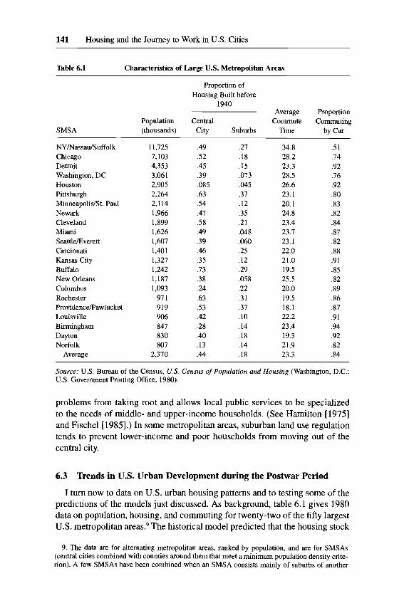
Table 6.1 Characteristics of Large U.S. Metropolitan Areas

SMSA

Proportion of Housing Built before

1940 Average Proportion

Population Central Commute Commuting (thousands) City Suburbs Time by Car

NYNassadSuffolk Chicago Detroit Washington, DC Houston Pittsburgh Minneapolis/St. Paul Newark Cleveland Miami SeattleEverett Cincinnati Kansas City Buffalo New Orleans Columbus Rochester Providenceh'awtucket Louisville Birmingham Dayton Norfolk

Average

1 1,725 7,103 4,353 3,061 2,905 2,264 2,114 1,966 1,899 1,626 1,607 1,401 1,327 1,242 1,187 1,093

97 1 919 906 847 830 807

2,370

.49

.52

.45

.39 ,085 .63 .54 .47 .58 .49 .39 .46 .35 .73 .38 .24 .63 .53 .42 .28 .40 .I3 .44

.27

. I8

.I5 ,073 ,045 .37 .12 .35 .21 .048 ,060 .25 .12 .29 ,058 .22 .31 .37 .I0 .14 . I 8 .I4 .18

34.8 28.2 23.3 28.5 26.6 23.1 20.1 24.8 23.4 23.7 23.1 22.0 21 .o 19.5 25.5 20.0 19.5 18.1 22.2 23.4 19.3 21.9 23.3

.5 1

.74

.92

.76

.92

.80 3 3 .82 .84 .87 3 2 .88 .91 .85 .82 .89 .86 .87 .91 .94 .92 .82 3 4

Source: US. Bureau of the Census, US. Census of Population and Housing (Washington, D.C.: U.S. Government Printing Office, 1980).

problems from taking root and allows local public services to be specialized to the needs of middle- and upper-income households. (See Hamilton [1975] and Fischel [1985].) In some metropolitan areas, suburban land use regulation tends to prevent lower-income and poor households from moving out of the central city.

6.3 Trends in U.S. Urban Development during the Postwar Period

I turn now to data on U.S. urban housing patterns and to testing some of the predictions of the models just discussed. As background, table 6.1 gives 1980 data on population, housing, and commuting for twenty-two of the fifty largest U.S. metropolitan areas.9 The historical model predicted that the housing stock

9. The data are for alternating metropolitan areas, ranked by population, and are for SMSAs (central cities combined with counties around them that meet a minimum population density crite- rion). A few SMSAs have been combined when an SMSA consists mainly of suburbs of another


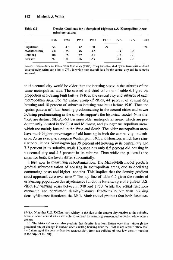
Table 6.2 Density Gradients for a Sample of Eighteen U.S. Metropolitan Areas (absolute values)

1948 1954 1958 1963 1970 1972 1977 1980

Population ,518 .47 .42 .38 .29 .24 Manufacturing .68 .55 .48 .42 .34 .32 Retailing .88 .75 .59 .44 .35 .30 Services .97 .81 .66 .53 .41 .38

Sources: These data are taken from Macauley (1985). They are estimated by the two-point method developed by Mills and Ohta (1976), in which only overall data for the central city and its suburbs are used.

in the central city would be older than the housing stock in the suburbs of the same metropolitan area. The second and third columns of table 6.1 give the proportion of housing built before 1940 in the central city and suburbs of each metropolitan area. For the entire group of cities, 44 percent of central city housing and 18 percent of suburban housing was built before 1940. Thus the spatial pattern of older housing predominating in the central cities and newer housing predominating in the suburbs supports the historical model. Note that there are distinct differences between older metropolitan areas, which are pre- dominantly located in the East and Midwest, and younger metropolitan areas, which are mainly located in the West and South. The older metropolitan areas have much higher percentages of old housing in both the central city and suburbs. As an example, compare Washington, DC, and Houston, which have similar populations. Washington has 39 percent old housing in its central city and 7.3 percent in its suburbs, while Houston has only 8.5 percent old housing in its central city and 4.5 percent in its suburbs. Thus while the pattern is the same for both, the levels differ substantially.

I turn now to measuring suburbanization. The Mills-Muth model predicts gradual suburbanization of housing in metropolitan areas, due to declining commuting costs and higher incomes. This implies that the density gradient must approach zero over time.'O The top line of table 6.2 gives the results of estimating population density/distance functions for a sample of eighteen U.S. cities for varying years between 1948 and 1980. While the actual functions estimated are population density/distance functions rather than housing density/distance functions, the Mills-Muth model predicts that both functions

SMSA. Note that U.S. SMSAs vary widely in the size of the central city relative to the suburbs, because some central cities are able to expand by annexing surrounded suburbs, while others are not.

10. The historical model also predicts that density functions flatten over time, although the predicted rate of change is slower since existing housing near the CBD is not rebuilt. Therefore the flattening of the density function results solely from the building of new low-density housing at the edge of the city.


will have the same density gradient as long as household size does not vary systematically with distance from the CBD. The results show that population density decreased by .58 per mile of distance in 1948, but the rate of decrease had dropped by more than half, to .24 per mile, by 1980. Thus housing in U.S. cities has suburbanized substantially during the postwar period.

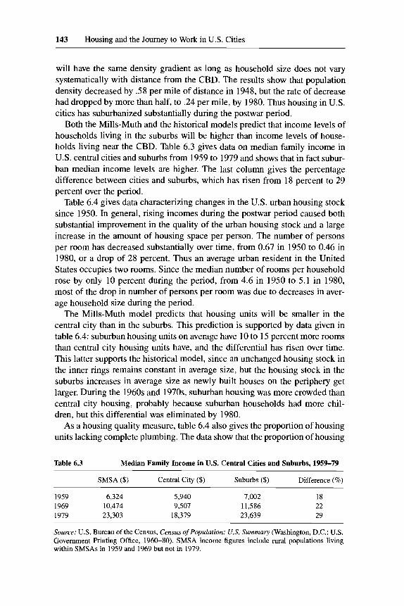
Both the Mills-Muth and the historical models predict that income levels of households living in the suburbs will be higher than income levels of households living near the CBD. Table 6.3 gives data on median family income in U.S. central cities and suburbs from 1959 to 1979 and shows that in fact suburban median income levels are higher. The last column gives the percentage difference between cities and suburbs, which has risen from 18 percent to 29 percent over the period.

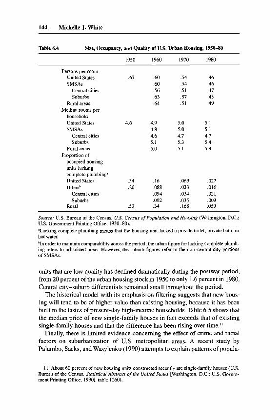
Table 6.4 gives data characterizing changes in the U.S. urban housing stock since 1950. In general, rising incomes during the postwar period caused both substantial improvement in the quality of the urban housing stock and a large increase in the amount of housing space per person. The number of persons per room has decreased substantially over time, from 0.67 in 1950 to 0.46 in 1980, or a drop of 28 percent. Thus an average urban resident in the United States occupies two rooms. Since the median number of rooms per household rose by only 10 percent during the period, from 4.6 in 1950 to 5.1 in 1980, most of the drop in number of persons per room was due to decreases in average household size during the period.

The Mills-Muth model predicts that housing units will be smaller in the central city than in the suburbs. This prediction is supported by data given in table 6.4: suburban housing units on average have 10 to 15 percent more rooms than central city housing units have, and the differential has risen over time. This latter supports the historical model, since an unchanged housing stock in the inner rings remains constant in average size, but the housing stock in the suburbs increases in average size as newly built houses on the periphery get larger. During the 1960s and 1970s, suburban housing was more crowded than central city housing, probably because suburban households had more children, but this differential was eliminated by 1980.

As a housing quality measure, table 6.4 also gives the proportion of housing units lacking complete plumbing. The data show that the proportion of housing

Table 6.3 Median Family Income in U.S. Central Cities and Suburbs, 1959-79

SMSA ($4 Central City ($) Suburbs ($) Difference (%)

1959 6,324 5,940 7,002 18 1969 10,474 9,507 11,586 22 1979 23,303 18,379 23,639 29

Source: U S . Bureau of the Census, Census of Population: U S . Summary (Washington, D.C.: US. Government Printing Office, 1960-80). SMSA income figures include rural populations living within SMSAs in 1959 and 1969 but not in 1979.


Table 6.4 Size, Occupancy, and Quality of U.S. Urban Housing, 1950-80

1950 1960 1970 1980

Persons per room United States SMSAs

Central cities Suburbs

Rural areas Median rooms per

household United States SMSAs


Rural areas Proportion of

occupied housing units lacking complete plumbing' United States Urbanb


Rural

.61

4.6

.34

.20

.53

.60

.60

.56

.63

.64

4.9 4.8 4.6 5.1 5.0

.16 ,088 ,094 .092 .34

.54

.54

.5 1

.57

.5 1

5.0 5.0 4.7 5.3 5.1

.069 ,033 ,034 .035 . I68

.46

.46

.47

.45

.49

5.1 5.1 4.7 5.4 5.3

.027 ,016 .021 .009 .059

Source: U.S. Bureau of the Census, US. Census of Population and Housing (Washington, D.C.: U.S. Government Printing Office, 1950-80). "Lacking complete plumbing means that the housing unit lacked a private toilet, private bath, or hot water.

order to maintain comparability across the period, the urban figure for lacking complete plumbing refers to urbanized areas. However, the suburb figures refer to the non-central city portions of SMSAs.

units that are low quality has declined dramatically during the postwar period, from 20 percent of the urban housing stock in 1950 to only 1.6 percent in 1980. Central city-suburb differentials remained small throughout the period.

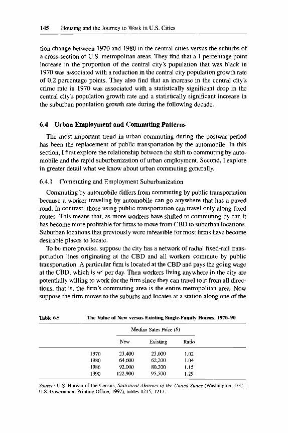
The historical model with its emphasis on filtering suggests that new housing will tend to be of higher value than existing housing, because it has been built to the tastes of present-day high-income households. Table 6.5 shows that the median price of new single-family houses in fact exceeds that of existing single-family houses and that the difference has been rising over time. "

Finally, there is limited evidence concerning the effect of crime and racial factors on suburbanization of U.S. metropolitan areas. A recent study by Palumbo, Sacks, and Wasylenko (1990) attempts to explain patterns of popula-

11. About 60 percent of new housing units constructed recently are single-family houses (U.S. Bureau of the Census, Statistical Abstract of the United States [Washington, D.C.: U.S. Govern- ment Printing Office, 19901, table 1260).


tion change between 1970 and 1980 in the central cities versus the suburbs of a cross-section of U.S. metropolitan areas. They find that a 1 percentage point increase in the proportion of the central city’s population that was black in 1970 was associated with a reduction in the central city population growth rate of 0.2 percentage points. They also find that an increase in the central city’s crime rate in 1970 was associated with a statistically significant drop in the central city’s population growth rate and a statistically significant increase in the suburban population growth rate during the following decade.

6.4 Urban Employment and Commuting Patterns

The most important trend in urban commuting during the postwar period has been the replacement of public transportation by the automobile. In this section, I first explore the relationship between the shift to commuting by automobile and the rapid suburbanization of urban employment. Second, I explore in greater detail what we know about urban commuting generally.

6.4.1 Commuting and Employment Suburbanization

Commuting by automobile differs from commuting by public transportation because a worker traveling by automobile can go anywhere that has a paved road. In contrast, those using public transportation can travel only along fixed routes. This means that, as more workers have shifted to commuting by car, it has become more profitable for firms to move from CBD to suburban locations. Suburban locations that previously were infeasible for most firms have become desirable places to locate.

To be more precise, suppose the city has a network of radial fixed-rail transportation lines originating at the CBD and all workers commute by public transportation. A particular firm is located at the CBD and pays the going wage at the CBD, which is w‘ per day. Then workers living anywhere in the city are potentially willing to work for the firm since they can travel to it from all directions, that is, the firm’s commuting area is the entire metropolitan area. Now suppose the firm moves to the suburbs and locates at a station along one of the

Table 6.5 The Value of New versus Existing Single-Family Houses, 1970-90

Median Sales Price ($)

New Existing Ratio

1970 23,400 23,000 1.02 1980 64,600 62,200 1.04 1986 92,000 80,300 1.15 1990 122,900 95,500 1.29

Source: U.S. Bureau of the Census, Statistical Absrract of the United States (Washington, D.C.: U.S. Government Printing Office, 1992), tables 1215, 1217.


radial routes. At the suburban location, the firm pays a wage equal to the wage at the CBD, wc, minus the cost of commuting between the firm’s suburban site and the CBD, tTx. Here tr is the (time plus out-of-pocket) cost of commuting a mile by rail in each direction, and x is the distance between the suburban firm and the CBD. Since the suburban firm has reduced its wage by the full cost of commuting between itself and the CBD, only workers who save this entire amount would be willing to work there. Workers who fit this condition live along the same radial transportation route as the suburban firm, but farther away from the CBD. They are indifferent between working for the suburban firm and working at the CBD, since wages net of commuting costs are equal at both job locations.12 Thus the firm’s commuting area once it moves to the suburbs becomes very restricted since it includes only workers who live along the same radial commuting line but farther from the CBD. As a result, moving to the suburbs is attractive only to very small firms.

Alternatively, the firm could move to the same suburban location but enlarge its commuting area by paying a higher wage. A higher wage would encourage workers located along the same line but closer in than x’ to out-commute to the firm. For example, if the suburban firm offers to pay the CBD wage wc, then a worker living halfway between the firm and the CBD will be just willing to out-commute to the firm. Workers living between the firm and the CBD but closer to the firm will prefer work at the firm over work at the CBD. Suppose the firm still needs more workers. It can raise its wage yet further, but eventu- ally it will have to attract workers who live along other rail lines. These workers must commute to the firm by traveling to the CBD along one line and then traveling away from the CBD to the firm along another. This requires a change of trains at the CBD, which is time-consuming and must be compensated by a large wage increase at the suburban firm. What all this suggests is that moving to the suburbs will be attractive only to small firms. Further, firms that move to the suburbs when commuting is by rail must locate near rail stations. But land within walking distance of suburban rail stations is scarce, which makes it expensive. This implies that firms receive little benefit in the form of lower land prices when they move out of the CBD.

Now suppose the number of public transit routes increases, perhaps by adding circumferential routes in addition to the existing radial routes. Then suburban locations would become more attractive to firms, either because additional public transit stations increase the number of suburban sites for firms or because more suburban sites are located at the intersection of two transit routes. The latter increases firms’ commuting areas for the same wage, since workers can commute to the firm from four rather than two directions without having to transfer. But the general picture remains that firms locating in the suburbs

12. Workers can be shown to maximize utility by choosing the job location that maximizes wages net of commuting costs when housing densities are assumed to be fixed (White 1990).


have relatively small commuting areas and that the cost in terms of higher wages of enlarging their commuting areas is high.

Now suppose most workers shift to commuting by car. All suburban locations are now accessible. This in itself makes moving out of the CBD more profitable, since suburban employment sites are less scarce and therefore cheaper. Also workers can commute to the firm along any road. This means that all suburban sites are in effect located at the intersection of several commuting routes, which makes them as accessible as sites located at the junction of several fixed-rail transportation lines. Also, there is never any need to com- pensate workers for the cost of waiting for buses or subways or for the cost of changing from one route to another. Therefore the cost to the firm in higher wages of a given expansion in its commuting area is smaller. In addition, the fact that commuting by car is faster expands the firm’s commuting area for a given wage. Therefore when workers commute by car rather than by public transportation, moving to the suburbs becomes much more attractive for firms, particularly large firms (White 1988a, 1990).

Suburbanization of employment in metropolitan areas can be measured using an employment density/distance function similar to the population density/ distance functions discussed above. Again the main parameter of interest is the density gradient, which measures the rate of decrease of employment density per mile of distance from the CBD. Table 6.2 also gives the results of estimating employment-density gradients for a group of U.S. cities during the postwar period. It shows that there has been rapid suburbanization of employment. The density gradient for manufacturing jobs fell from .68 in 1948 to .32 in 1977, a decrease of over 50 percent. The density gradients in retailing and services fell even more rapidly, although the decline occurred somewhat later. In general, employment was much more centralized than housing at the beginning of the postwar period, but suburbanization of employment has proceeded more rapidly during the period, so that the density gradients for housing and employment are now approaching one another.

In explaining this trend, commentators often have stressed the attractiveness of lower suburban land prices to firms. When firms rent or buy sites in the CBD, the opportunity cost of the site is use by another firm, so that land values are high, while when they rent or buy suburban sites, the opportunity cost of a site is its value used for housing, which is much lower. Suburban land has always been cheaper than land near the CBD, however; in fact it was cheaper relative to CBD land in the past than it is currently. The shift by workers from commuting by public transportation to commuting by automobile made it possible for firms to benefit from the suburbs’ lower land prices.I3

13. The cost of transporting inputs and outputs has also fallen, and the urban export node for most firms is no longer located at the CBD. Both of these factors have also made suburban sites more attractive to firms.


The suburbanization of housing documented in section 6.3 would necessar- ily have lengthened workers’ commuting journeys if all firms had remained at the CBD. However, suburbanization of jobs has an offsetting effect on the length of workers’ commuting journeys. Increased employment suburbanization has in turn encouraged additional housing suburbanization, because workers having jobs in the near suburbs of a metropolitan area can live in the far suburbs of the same metropolitan area, where housing prices are particularly low, and have commuting journeys that take no longer than the commute from the near suburbs to the CBD. Thus employment suburbanization has encouraged the growth of new suburban rings on the periphery of the metropolitan area. As a result, the largest U.S. metropolitan areas have grown to the point that the farthest suburbs may be located fifty miles or more from the CBD. Few workers commute as far as this, though, since most residents of the far suburbs work at jobs in nearer suburbs. As cities have grown and employment has suburbanized, jobs at the CBD have become less and less attractive, since workers who commute to the CBD from the suburbs must cross congested suburban employment subcenters along the way as well as experiencing the congestion around the CBD itself. The result is that few jobs are located at the CBD. For the fifty largest U.S. metropolitan areas, only 8 percent of jobs on average are located at the CBD.

Urban roads are undeniably congested at the peak rush hours, and the popular press often suggests that congestion has been getting worse over time. It should be noted, however, that some level of congestion is efficient. Suppose road systems were designed to minimize the total cost of travel, including drivers’ time cost and the cost of constructing and maintaining roads. Then the optimal road capacity, measured in lanes, would occur where the marginal cost of increasing traffic capacity by widening the road equals the marginal cost of increasing traffic capacity by increasing the level of congestion. Since the cost of widening roads is high, the marginal cost of congestion must also be high at the optimum road width.

6.4.2 The Shift from Public Transportation to Automobile Commuting

In this section, I document the shift from public transportation to automobile commuting and other aspects of urban commuting and urban travel generally.

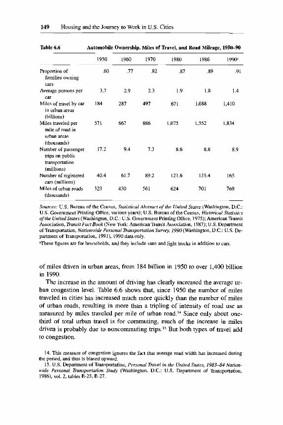
Table 6.6 gives data on automobile ownership since 1950. It shows that, while automobile ownership was already widespread by 1950, when 60 percent of families owned cars, it had became nearly universal by the late 1980s, when about 90 percent owned cars. More important, the average number of persons per vehicle has fallen drastically, from 3.7 in 1950 to only 1.4 in 1990. (The 1990 figure includes light trucks and vans owned by households.) Since these figures include children, the elderly, and other nondrivers, they imply that most households now have a vehicle for each driver. The increase in the number of vehicles was accompanied by an enormous increase in the total number


Table 6.6 Automobile Ownership, Miles of Travel, and Road Mileage, 1950-90

1950 1960 1970 1980 1986 1990"

Proportion of families owning

Average persons per

Miles of travel by car

cars

Car

in urban areas (billions)

Miles traveled per mile of road in urban areas (thousands)

trips on public transportation (millions)

Number of registered cars (millions)

Miles of urban roads (thousands)

Number of passenger

.60

3.7

184

57 1

17.2

40.4

323

.77

2.9

287

667

9.4

61.7

430

.82

2.3

497

886

7.3

89.2

561

.87

I .9

67 1

1,075

8.6

121.6

624

.89

1.8

1,088

1,552

8.8

135.4

701

.91

1.4

1,410

1,834

8.9

165

769

Sources: U.S. Bureau of the Census, Statistical Abstract ofthe United States (Washington, D.C.: U.S. Government Printing Office, various years); U.S. Bureau of the Census, Historical Statistics ofthe United States (Washington, D.C.: U.S. Government Printing Office, 1975); American Transit Association, Transit Fact Book (New York: American Transit Association, 1987); U.S. Department of Transportation, Nationwide Personal Transportation Survey, I990 (Washington, D.C.: US. De- partment of Transportation, 1991). 1990 data only. "These figures are for households, and they include vans and light trucks in addition to cars.

of miles driven in urban areas, from 184 billion in 1950 to over 1,400 billion in 1990.

The increase in the amount of driving has clearly increased the average urban congestion level. Table 6.6 shows that, since 1950 the number of miles traveled in cities has increased much more quickly than the number of miles of urban roads, resulting in more than a tripling of intensity of road use as measured by miles traveled per mile of urban road.I4 Since only about one- third of total urban travel is for commuting, much of the increase in miles driven is probably due to noncommuting trips.I5 But both types of travel add to congestion.

14. This measure of congestion ignores the fact that average road width has increased during the period, and thus is biased upwwd.

15. US. Department of Transportation, Personal Travel in the United States, 1983-84 Nution- wide Personal Transportation Study (Washington, D.C.: U.S. Department of Transportation, 1986), vol. 2, tables E-23, E-27.


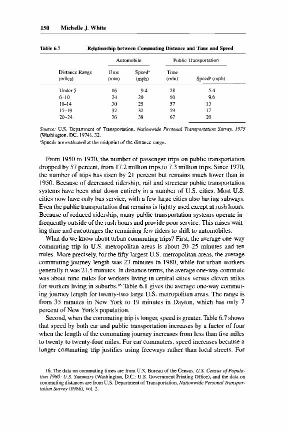
Table 6.7 Relationship between Commuting Distance and Time and Speed

Automobile Public Transportation

Distance Range Time Speed’ Time (miles) (min) (mph) (fin) Speed” (mph)

Under 5 16 9.4 28 5.4 6-1 0 24 20 50 9.6 11-14 30 25 57 13 15-19 32 32 59 17 20-24 36 38 67 20

Source: U S . Department of Transportation, Nationwide Personal Transportation Survey, 1973 (Washington, DC, 1974). 32. “Speeds are evaluated at the midpoint of the distance range.

From 1950 to 1970, the number of passenger trips on public transportation dropped by 57 percent, from 17.2 million trips to 7.3 million trips. Since 1970, the number of trips has risen by 21 percent but remains much lower than in 1950. Because of decreased ridership, rail and streetcar public transportation systems have been shut down entirely in a number of U.S. cities. Most US. cities now have only bus service, with a few large cities also having subways. Even the public transportation that remains is lightly used except at rush hours. Because of reduced ridership, many public transportation systems operate in- frequently outside of the rush hours and provide poor service. This raises waiting time and encourages the remaining few riders to shift to automobiles.

What do we know about urban commuting trips? First, the average one-way commuting trip in U.S. metropolitan areas is about 20-25 minutes and ten miles. More precisely, for the fifty largest U.S. metropolitan areas, the average commuting journey length was 23 minutes in 1980, while for urban workers generally it was 21.5 minutes. In distance terms, the average one-way commute was about nine miles for workers living in central cities versus eleven miles for workers living in suburbs.I6 Table 6.1 gives the average one-way commuting journey length for twenty-two large U.S. metropolitan areas. The range is from 35 minutes in New York to 19 minutes in Dayton, which has only 7 percent of New York’s population.

Second, when the commuting trip is longer, speed is greater. Table 6.7 shows that speed by both car and public transportation increases by a factor of four when the length of the commuting journey increases from less than five miles to twenty to twenty-four miles. For car commuters, speed increases because a longer commuting trip justifies using freeways rather than local streets. For

16. The data on commuting times are from U.S. Bureau of the Census, U.S. Census of Populu- tion 1980: U.S. Surnrnaly (Washington, D.C.: U.S. Government Printing Office), and the data on commuting distances are from U.S. Department of Transportation, Nationwide Personal Trunspor- tation Survey (1986), vol. 2.


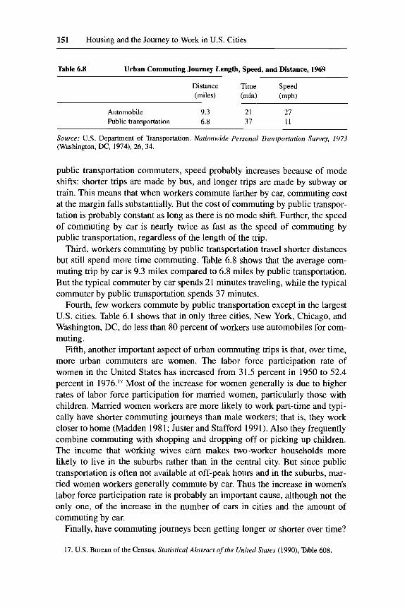
Table 6.8 Urban Commuting Journey Length, Speed, and Distance, 1969

Distance Time Speed (miles) (min) (mph)

Automobile 9.3 21 21 Public transportation 6.8 37 11

Source: U S . Department of Transportation, Nationwide Personal Transportation Survey, 1973 (Washington, DC, 1974). 26,34.

public transportation commuters, speed probably increases because of mode shifts: shorter trips are made by bus, and longer trips are made by subway or train. This means that when workers commute farther by car, commuting cost at the margin falls substantially. But the cost of commuting by public transportation is probably constant as long as there is no mode shift. Further, the speed of commuting by car is nearly twice as fast as the speed of commuting by public transportation, regardless of the length of the trip.

Third, workers commuting by public transportation travel shorter distances but still spend more time commuting. Table 6.8 shows that the average commuting trip by car is 9.3 miles compared to 6.8 miles by public transportation. But the typical commuter by car spends 21 minutes traveling, while the typical commuter by public transportation spends 37 minutes.

Fourth, few workers commute by public transportation except in the largest U.S. cities. Table 6.1 shows that in only three cities, New York, Chicago, and Washington, DC, do less than 80 percent of workers use automobiles for commuting.

Fifth, another important aspect of urban commuting trips is that, over time, more urban commuters are women. The labor force participation rate of women in the United States has increased from 31.5 percent in 1950 to 52.4 percent in 1976.” Most of the increase for women generally is due to higher rates of labor force participation for married women, particularly those with children. Married women workers are more likely to work part-time and typically have shorter commuting journeys than male workers; that is, they work closer to home (Madden 1981; Juster and Stafford 1991). Also they frequently combine commuting with shopping and dropping off or picking up children. The income that working wives earn makes two-worker households more likely to live in the suburbs rather than in the central city. But since public transportation is often not available at off-peak hours and in the suburbs, married women workers generally commute by car. Thus the increase in women’s labor force participation rate is probably an important cause, although not the only one, of the increase in the number of cars in cities and the amount of commuting by car.

Finally, have commuting journeys been getting longer or shorter over time?

17. U S . Bureau of the Census, Statistical Abstract of the United States (1990), Table 608.


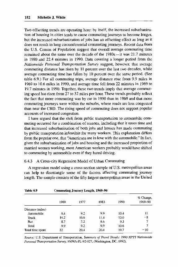
Two offsetting trends are operating here: by itself, the increased suburbanization of housing in cities tends to cause commuting journeys to become longer, but the increased suburbanization of jobs has an offsetting effect as long as it does not result in long circumferential commuting journeys. Recent data from the U.S. Census of Population suggest that overall average commuting time remained about the same over the decade of the 1980s-it was 21.7 minutes in 1980 and 22.4 minutes in 1990. Data covering a longer period from the Nationwide Personal Transportation Survey suggest, however, that average commuting distance has risen by 11 percent over the last two decades, while average commuting time has fallen by 10 percent over the same period. (See table 6.9.) For all commuting trips, average distance rose from 9.9 miles in 1969 to 10.6 miles in 1990, and average time fell from 22 minutes in 1969 to 19.7 minutes in 1990. Together, these two trends imply that average commuting speed has risen from 27 to 32 miles per hour. These trends probably reflect the fact that more commuting was by car in 1990 than in 1969 and that more commuting journeys were within the suburbs, where roads are less congested than near the CBD. The rising speed of commuting does not support popular accounts of increased congestion.

I have argued that the shift from public transportation to automobile commuting occurred for a combination of reasons, including that it saves time and that increased suburbanization of both jobs and houses has made commuting by public transportation infeasible for many workers. This explanation differs from the popular one, that “Americans are in love with the automobile.” In fact, given the suburbanization of jobs and housing and the increased proportion of married women working, most American workers probably would have shifted to commuting by automobile even if they hated driving.

6.4.3 A Cross-city Regression Model of Urban Commuting

A regression model using a cross-section sample of U.S. metropolitan areas can help to disentangle some of the factors affecting commuting journey length. The sample consists of the fifty largest metropolitan areas in the United

Table 6.9 Commuting Journey Length, 1969-90

% Change, 1969 1977 1983 1990 1969-90

Distance (miles) Automobile 9.4 9.2 9.9 10.4 11 Truck 14.2 10.6 11.4 13.0 -8 Bus 8.7 7.2 8.6 9.3 I Total 9.9 9.2 9.9 10.6 I

Total time spent 22 20.4 20.4 19.7 - 10

Source: U S . Department of Transportation, Summary of Travel Trends: I990 NPTS Nationwide Personal Transportation Survey, FHWA-PL-92-027, (Washington, DC, 1992).


States in 1980. The dependent variable is average time spent commuting, in minutes. Measuring commuting journey length in terms of time rather than distance is preferable, since the major resource cost of commuting is its time cost rather than its out-of-pocket cost. Average commuting journey length is hypothesized to depend on population of the metropolitan area (POP) , median income per person in the metropolitan area (MEDZNC), the proportion of workers in the metropolitan area who are black (BLACK), the proportion of workers in the metropolitan area who use public transportation (PUBTRAN), the proportion of jobs in the metropolitan area located at the CBD (CBDJOBS), the proportion of households in the metropolitan area who have moved within the last five years (MOVER), and the proportion of households in which both the husband and wife work (2 WHH).

Higher urban population is expected to raise the average commuting journey length, since larger cities tend to be more spread out. However, while population suburbanization increases average commuting journey length, employment suburbanization tends to have an offsetting effect. The proportion of jobs located at the CBD is a measure, albeit quite crude, of employment centraliza- tion, so that its coefficient is expected to be positive. Higher household income is expected to be associated with higher average commuting journey length, since higher-income households tend to prefer suburban housing. Cities having greater use of public transportation are expected to have longer commuting times, since commuting by public transportation is slower than commuting by car. Cities with more black workers are expected to have higher average commuting journey length. This is because black workers are likely to live near the CBD, while many jobs have moved to the suburbs. This means that black workers often have long out-commuting journeys that are slow. The variable MOVER could have either sign. Workers may change residential locations in order to be closer to their jobs, which would make the sign of MOVER negative. But workers may also move because their incomes have risen, in which case they are likely to locate farther out, making the sign of MOVER positive. Which effect predominates is an empirical question. Since married women workers have shorter commuting journeys than other workers, an increase in the proportion of two-worker households is expected to reduce the average commuting journey length.

The results are shown in table 6.10. The constant term is 10 minutes, indicat- ing a significant fixed time component to commuting, regardless of mode. The population variable ( P O P ) is positive and significant, but small. An increase in the metropolitan area population of one million people increases the average commuting journey length by only 0.4 minutes. This suggests that employment suburbanization in large cities has almost, but not fully, offset the effect of population suburbanization in raising commuting journey length. The percentage of jobs at the CBD has the expected positive sign but is insignificant. Use of public transportation for commuting carries a large time disadvantage: if all of a city’s workers commuted by public transportation rather than by car, the


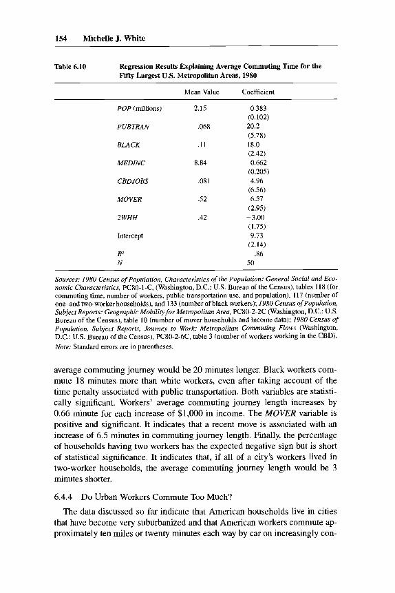
Table 6.10 Regression Results Explaining Average Commuting Time for the Fifty Largest U.S. Metropolitan Areas, 1980

Mean Value Coefficient

POP (millions) 2.15 0.383

PUBTRAN ,068 20.2 (5.78)

BLACK . I 1 18.0 (2.42)

MEDINC 8.84 0.662 (0.205)

CBDJOBS ,081 4.96 (6.56)

MOVER .52 6.57 (2.95)

2 WHH .42 -3.00 (1.75)

(2.14)

(0.102)

Intercept 9.73

Rl .86 N 50

Sources: 1980 Census of Population, Characteristics of the Population: General Social and Eco- nomic Characteristics, PCSO-I-C, (Washington, D.C.: U.S. Bureau of the Census), tables 118 (for commuting time, number of workers, public transportation use, and population), 117 (number of one- and two-worker households), and 133 (number of black workers); 1980 Census ofPopulation, Subject Reports: Geographic Mobility for Metropolitan Area, PC80-2-2C (Washington, D.C.: US. Bureau of the Census), table 10 (number of mover households and income data); 1980 Census oj Population, Subject Reports, Journey to Work: Metropolitan Commuting Flows (Washington, D.C.: US. Bureau of the Census), PC80-2-6C, table 3 (number of workers working in the CBD). Note: Standard errors are in parentheses.

average commuting journey would be 20 minutes longer. Black workers commute 18 minutes more than white workers, even after taking account of the time penalty associated with public transportation. Both variables are statistically significant. Workers’ average commuting journey length increases by 0.66 minute for each increase of $1,000 in income. The MOVER variable is positive and significant. It indicates that a recent move is associated with an increase of 6.5 minutes in commuting journey length. Finally, the percentage of households having two workers has the expected negative sign but is short of statistical significance. It indicates that, if all of a city’s workers lived in two-worker households, the average commuting journey length would be 3 minutes shorter.

6.4.4

The data discussed so far indicate that American households live in cities that have become very suburbanized and that American workers commute ap- proximately ten miles or twenty minutes each way by car on increasingly con-

Do Urban Workers Commute Too Much?


gested roads, regardless of whether they live in large or small cities. Does this suggest that urban workers in the United States commute too much?

One reason to think that urban workers commute too much is that automobile travel is underpriced generally and the underpricing is more severe on congested urban roads used by commuters. While drivers pay for the cost of purchasing and operating automobiles, they do not pay the full cost of building and maintaining highways (although they do pay excise taxes on gasoline, which in turn pay for part of the cost of roads). In addition, urban drivers do not bear the costs of congestion and air pollution that extra driving produces. In a recent paper (White 1990), I quantified this externality and found that central city rush hour driving is underpriced by around 44 percent and suburban rush hour driving by around 18 percent. The lower suburban figure results from lower congestion levels in the suburbs. This underpricing of urban driving gives workers an incentive to commute too much. The obvious policy measure to deal with the underpricing of urban driving would be congestion tolls collected only on congested roads during rush hours. But no U.S. jurisdiction has ever tried this approach.18

Hamilton (1982) first raised the question of whether urban commuting is “wasteful” in the sense that the aggregate amount of commuting could be reduced, without changing the spatial pattern of jobs and housing, by pairs of workers trading jobs or houses. The efficient amount of commuting is the minimum necessary to connect the metropolitan area’s existing houses with its existing jobs. Any commuting in excess of this amount is wastef~1.I~ Note that the question as posed assumes that the dispersed land use pattern in U.S. cities is efficient, both for jobs and housing. It thus ignores any distortions in the land use pattern that might be caused by such factors as the underpricing of road use or of gasoline.

Efficient commuting includes both radial and circumferential commuting. Circumferential commuting is efficient when a group of firms or a single large firm locates at a particular point in the suburbs, presumably to take advantage of agglomeration economies or economies of scale. This makes it necessary for workers to commute to these firms from around the metropolitan area, since more jobs are offered than there are workers living along the same ray from the CBD. Thus a nonuniform distribution of suburban jobs in different directions around the CBD implies that some amount of circumferential commuting must be efficient.

White (1988b) developed an approach by which actual commuting could be separated into efficient versus wasteful commuting, using an assignment

18. The city of Singapore levies a toll on drivers who enter the CBD during the day. 19. Not all “wasteful” commuting would he considered to be inefficient in an economic model.

For example, if a household chooses to live in a particular neighborhood that requires its worker to make a long out-commuting trip, then the trip would be wasteful according to the definition given here, but would not be economically inefficient unless the household’s choice were distorted by some factor such as rent control, zoning, or transportation subsidies.


For each city analyzed, I used data consisting of the number of jobs in each geographical subdivision of the metropolitan area, the number of houses in each subdivision of the metropolitan area, a matrix of actual commuting times to get from each subdivision to every other subdivision, and a matrix of the number of workers that live in each subdivision and work in every other subdivision (actual commuting flows). Using the two matrices of actual commuting flows and actual commuting times, the average actual commuting journey length can be calculated. Then an assignment model was used to deter- mine a new, optimal matrix of commuting flows that minimizes total time spent commuting for all workers in the metropolitan areas, taking as given the actual number of jobs and houses in each subdivision. From the matrix of optimal commuting flows, the average efficient commuting journey can be computed. The difference between efficient commuting and actual commuting is the amount of wasteful commuting.21

I found that wasteful commuting constituted only around 10 percent of total urban commuting-a surprisingly low figure. The results of the assignment model typically resulted in an efficient commuting pattern in which most workers work in the same jurisdiction in which they live or in the neighboring jurisdiction, and excess suburban workers commute to the CBD. Out- commuting and circumferential commuting journeys were eliminated by trading.

The result that only a small fraction of urban commuting in the United States is wasteful is subject to two major criticisms. First, the assignment model treats all workers and all jobs in the metropolitan area as identical. Obviously in the real world, workers and jobs are not homogeneous, so that many such trades would not be possible. In particular, the model ignores the special commuting circumstances faced by black workers and by working couples. Black workers may live near the CBD because housing discrimination reduces opportunities to live anywhere else, but they may make long out-commuting journeys because most job opportunities are in the suburbs. The assignment model treats these trips as wasteful and eliminates them by trading jobs or residences. Simi- larly, workers in two-worker households may make circumferential or out- commuting journeys because they choose to live halfway between their two jobs. The assignment model separates couples so as to reduce commuting by assigning each worker separately. Further, households often are attached to their neighborhoods and their jobs and prefer to commute more in order to avoid change. These two latter factors tend to bias my wasteful commuting results upward.

On the other hand, I used census data for my study, and this means that

20. Hamilton (1982) also developed a methodology to separate commuting into efficient versus wasteful commuting, but his methodology was flawed since it assumed that all circumferential commuting was wasteful. See also Hamilton (1990).

21. Note that census data are available only for commuting time, not commuting distance.


data were available for only a relatively small number of subdivisions in each metropolitan area. But the assignment model implicitly assumes that any commuting journeys by workers who both live and work in the same subdivision are efficient. It therefore ignores any wasteful commuting that could be identified if the unit of analysis were smaller. In particular, census data treat the central cities of most SMSAs as one subdivision, although the CBD is a separate unit. More recent research using the same approach has taken advantage of transportation surveys for particular cities that identify a much larger number of subdivisions. Thus, for example, Clopper and Gordon (1991) estimated an assignment model for Baltimore with data that identified five hundred subdivisions and found that about half the amount of commuting, measured in terms of distance, was wasteful. This suggests that while urban models- which predict that workers themselves will tend to minimize commuting given the spatial pattern of jobs and housing-do a reasonably good job of explaining commuting behavior, the relatively low cost of travel in the United States allows workers to trade off longer commuting trips against many other objectives.

6.5 What Lies Ahead?

The historical model discussed above suggests that suburban housing, like central city housing, will decay as it ages, causing central city problems to appear in the suburbs. Such a pattern has been observed in some suburban areas, mainly where the suburbs of metropolitan areas surround subcenters that are in effect small central cities. The city of Yonkers in Westchester County, NY, is an example. Otherwise, most housing in suburban areas has seemed to grow old without decaying, and close-in suburbs in many metropolitan areas have appeared to benefit from their high accessibility to jobs. Part of the reason for this may be that suburban jurisdictions are inherently more stable than central cities because of their aggressive use of land use controls to regulate new development and keep out problems. This suggests that the decline in the quality of the housing stock in central cities may have occurred, not so much because of aging, but because of proximity to central city problems.

Continuing suburbanization suggests that metropolitan areas in the future will be even more spread out than today. They will also be less compact than in the past, with more vacant areas within the developed margin. The vacant areas may be either places where housing has been abandoned or areas that are subject to overly restrictive land use controls and have been skipped over. Metropolitan areas are likely to consist of widely scattered employment subcenters and scattered residential neighborhoods. If the price of gasoline rose drastically-either because of new taxes or a new oil crisis-jobs and residences would become more spatially integrated, but the trend toward amor- phous cities would probably continue.

Employment will also continue to suburbanize. Greater use of computers


and new forms of telecommunications are likely to reduce agglomeration economies, because there is less need for face-to-face contact and because parties can communicate and exchange documents quickly without being phys- ically close to each other. This change seems likely to further erode the attractiveness of CBDs as employment locations.

What about urban congestion? The data discussed here suggest that urban congestion has been getting better rather than worse, so it is not surprising that local government officials appear to be unconcerned about it. Ironically, the only serious proposals to do anything about urban congestion have come from the Environmental Protection Agency-the U.S. government agency responsi- ble for enforcing clean air laws. The EPA has proposed a number of drastic measures designed to clean up the air by reducing driving. In Los Angeles, it has proposed that a regional clean air authority be given power to shorten commuting journeys by directing new job growth to suburban areas where most new housing is currently being built and directing new housing growth to more central areas along the coast where most jobs in the Los Angeles re- gion are located. The latter is likely to be resisted by local officials, since high land costs on the coast make only high-density housing economically feasible, but apartments are barred by local zoning rules. The former is more feasible, since employment is suburbanizing rapidly anyway. Although jobs are likely to become more suburbanized and jobs and housing to become more balanced, however, commuting trips are likely to remain about the same length as they are now, regardless of what the EPA or other government agencies might try to do.

References

Clopper, M., and P. Gordon. 1991. Wasteful Commuting: A Reexamination. Journal of

Fischel, W. 1985. The Economics of Zoning Laws. Baltimore: Johns Hopkins Univer-

Hamilton, B. 1975. Zoning and Property Taxation in a System of Local Governments.

. 1982. Wasteful Commuting. Journal ef Political Economy 90: 1035-53.

Urban Economics 29:2-13.

sity Press.

Urban Studies 12:205-11.

. 1990. Wasteful Commuting Again. Journal of Political Economy 97: 1497- 1504.

Hanushek, E. 198 1. Throwing Money at Schools. Journal of Policy Analysis and Man- agement 1 : 19-41.

Harrison, D., and J. Kain. 1974. Cumulative Urban Growth and Urban Density Func- tions. Journal of Urban Economics 1:61-98.

Juster, T., and F. Stafford. 1991. The Allocation of Time: Empirical Findings, Behav- ioral Models, and Problems of Measurement. Journal of Economic Literature

LeRoy, S., and J. Sonstelie. 1983. Paradise Lost and Regained: Transportation Innova- 29:47 1-522.

tion, Income, and Residential Location. Journal of Urban Economics 13:67-89.

159 Housing and the Journey to Work in U S . Cities

Macaulay, M. 1985. Estimation and Recent Behavior of Urban Population and Employ-

McFadden, D. 1974. The Measurement of Urban Travel Demand. Journal of Public

Madden, J. 1981. Why Women Work Closer to Home. Urban Studies 18: 181-94. Mieszkowski, P., and G. Zodrow. 1989. Taxation and the Tiebout Model: The Differen-

tial Effects of Head Taxes, Taxes on Land Rents, and Property Taxes. Journal of Economic Literature 27: 1098-1 146.

Mills, E. 1972. Studies in the Structure of the Urban Economy. Baltimore: Johns Hop- kins University Press.

Mills, E., and K. Ohta. 1976. Urbanization and Urban Problems. In Asia’s New Giant: How the Japanese Economy Works, ed. H. Patrick and H. Rosovsky. Washington, D.C.: Brookings Institution.

ment Density Gradients. Journal of Urban Economics 18:25 1-60.

Economics 3:303-28.

Muth, R. 1969. Cities and Housing. Chicago: University of Chicago Press. Palumbo, G., S. Sacks, and M. Wasylenko. 1990. Population Decentralization within

Metropolitan Areas: 1970-1980. Journal of Urban Economics 27: 15 1-67. Polinsky, A. M., and D. Ellwood. 1979. An Empirical Reconciliation of Micro and

Grouped Estimates of the Demand for Housing. Review of Economics and Statis- tics 6 1 : 199-205.

Stemlieb, G., and R. Burchell. 1973. Residential Abandonment: The Tenement Lund- lord Revisited. New Brunswick, N.J.: Rutgers University Press.

Tiebout, C. 1956. A Pure Theory of Local Expenditures. Journal of Political Econ- omy 54:416-24.

Wheaton, W. 1982. Urban Residential Growth under Perfect Foresight. Journal of Ur- ban Economics 12: 1-21.

White, M. 1986. Property Taxes and Urban Housing Abandonment. Journal of Urban Economics 20:3 12-30.

. 1988a. Location Choice and Commuting Behavior in Cities with Decentralized Employment. Journal of Urban Economics 24: 129-52.

. 1988b. Urban Commuting Is Not ‘Wasteful.’ Journal of Political Economy

. 1990. Commuting and Congestion: A Simulation Model of a Decentralized Metropolitan Area. Journal of the American Real Estate and Urban Economics Asso- ciation 18:335-68.

96: 1097-1 110.

This Page Intentionally Left Blank

Housing and the Journey to Work in U.S. Cities · 6 Housing and the Journey to Work in U.S. Cities...

Documents

Transcript of Housing and the Journey to Work in U.S. Cities · 6 Housing and the Journey to Work in U.S. Cities...